point-based multiscale surface...

Point-Based Multiscale Surface Representation

MARK PAULY

Stanford University

LEIF P. KOBBELT

RWTH Aachen

and

MARKUS GROSS

ETH Zurich

In this article we present a new multiscale surface representation based on point samples. Given an unstructured point cloud

as input, our method first computes a series of point-based surface approximations at successively higher levels of smoothness,

that is, coarser scales of detail, using geometric low-pass filtering. These point clouds are then encoded relative to each other by

expressing each level as a scalar displacement of its predecessor. Low-pass filtering and encoding are combined in an efficient

multilevel projection operator using local weighted least squares fitting.

Our representation is motivated by the need for higher-level editing semantics which allow surface modifications at different

scales. The user would be able to edit the surface at different approximation levels to perform coarse-scale edits on the whole model

as well as very localized modifications on the surface detail. Additionally, the multiscale representation provides a separation in

geometric scale which can be understood as a spectral decomposition of the surface geometry. Based on this observation, advanced

geometric filtering methods can be implemented that mimic the effects of Fourier filters to achieve effects such as smoothing,

enhancement, or band-bass filtering.

Categories and Subject Descriptors: I.3.5 [Computer Graphics]: Computational Geometry and Object Modeling—Boundaryrepresentation, curve, surface, solid, and object representations

General Terms: Algorithms

Additional Key Words and Phrases: Surface representations, shape modeling, spectral filtering, morphing, scale space, geometric

modeling

1. INTRODUCTION

Shape modeling applications range from CAD for car and airplane design, e-commerce, and medicalapplications to character design for games and movies, and more. This variety in applications fieldsis reflected in a great diversity of shape modeling approaches and shape representations. The latterare often tailored to the specific needs of the application in mind. Due to hardware restrictions, mostearly surface representations were optimized for low memory usage, using higher order approximation

This work has been supported by the joint Berlin/Zurich graduate program Combinatorics, Geometry, and Computation, financed

by the ETH Zurich and the German Science Foundation (DFG).

Author’s address: M. Pauly, Institute for Computational Science, ETH Zurich, IFW C 26.2, Haldeneggsteig 4/Weinbergstrasse,

CH-8092 Zurich, Switzerland; email: [email protected].

Permission to make digital or hard copies of part or all of this work for personal or classroom use is granted without fee provided

that copies are not made or distributed for profit or direct commercial advantage and that copies show this notice on the first

page or initial screen of a display along with the full citation. Copyrights for components of this work owned by others than ACM

must be honored. Abstracting with credit is permitted. To copy otherwise, to republish, to post on servers, to redistribute to lists,

or to use any component of this work in other works requires prior specific permission and/or a fee. Permissions may be requested

from Publications Dept., ACM, Inc., 1515 Broadway, New York, NY 10036 USA, fax: +1 (212) 869-0481, or [email protected].

c© 2006 ACM 0730-0301/06/0400-0177 $5.00

ACM Transactions on Graphics, Vol. 25, No. 2, April 2006, Pages 177–193.

178 • M. Pauly et al.

or interpolation methods. Examples are tensor-product spline surfaces that were introduced in the 60sand are still widely used in commercial CAD systems. When memory became cheap and new special-ized graphics chips emerged, polygon-based surfaces, such as triangle meshes and subdivision surfaces,became dominant. Since the global consistency constraints of these surfaces are less restrictive, theyare more suited for handling simple as well as complex geometry, in particular, when the shape and/ortopology undergoes frequent changes during editing or simulation. Recently, point-based modeling hasbecome popular, taking the trend of reducing the global structure of a surface representation a stepfurther at the cost of using more and simpler modeling primitives. Initially proposed as a renderingprimitive [Levoy and Whitted 1985], point samples have also been used for shape and appearancemodeling [Pauly et al. 2003; Kalaiah and Varshney 2003; Zwicker et al. 2002]. Point-based representa-tions offer a number of advantages which are mainly the result of their structural simplicity and lackof a global connectivity graph or parameterization. Thus insertion, deletion, or repositioning of pointsamples is trivial which supports efficient, dynamic adaptation of the local sampling rate. This makespoint-based representations particularly suitable for dynamic settings where the geometry of the modeland/or the accuracy of the approximation changes frequently. Examples include large geometric defor-mations in shape modeling [Pauly et al. 2003] or simulation [Carlson et al. 2002; Feldman et al. 2003;Muller et al. 2004; Pauly et al. 2005], or level-of-detail representations [Pauly et al. 2002a].

This work extends previous point-based representations from a single-scale description of the modelsurface towards a true multiscale shape representation. The concept of scale is fundamental to hu-man perception. Hence scale-space methods have become increasingly popular and widespread in dataanalysis and modeling (see Lindeberg [1994] or Weickert [1998] for an overview). So far, scale-spacetechniques have mainly been applied to functional data such as sound, images, or flow fields. This workgoes beyond these earlier efforts in that it applies the concept of scale-space to irregularly sampled,discrete manifold surfaces. The main motivation is to enhance the description of a geometric model byexplicitly modeling surface detail at different geometric scales. Hence, our multiscale surface represen-tation provides a set of surface approximations at different levels of smoothness. This allows the userto manipulate a model in a flexible and intuitive way without having to pay close attention to whetheror not the surface detail is properly affected. Thus the user can freely choose on which level of scalehis editing operations should be applied, either coarse global edits on the general shape of the object ormodifications on the fine surface detail.

A key issue in the definition of a multiscale surface representation is the interconnection betweensuccessive levels in the hierarchy. To obtain intuitive editing semantics, it is essential that changesin one level are propagated naturally to the next higher levels [Kobbelt et al. 1998, 1999]. This canbe achieved by encoding each level of the discrete multiscale representation as a normal displacementof its immediate smoother approximation. Thus the difference between two successive levels can beexpressed as a set of scalar detail coefficients that approximates for each point the distance betweenthe two levels in normal direction [Kobbelt et al. 1998; Guskov et al. 1999; Zorin et al. 1997; Botschand Kobbelt 2004]. These detail coefficients can be considered as discrete frequency bands that allowspectral filtering methods to be applied to point-sampled models.

It is important to note the distinction between a multiscale and a multiresolution surface repre-sentation. The former describes a surface at different levels of smoothness without any reference toa particular sampling distribution. The latter, on the other hand, refers to a set of surface approxi-mations with varying sampling resolution, thus describing a surface at different levels of coarseness.Multiresolution surface representations have been used successfully in the context of efficient render-ing [Rossignac and Borrel 1993], surface compression and progressive transmission [Khodakovskyet al. 2000], surface analysis [Eck et al. 1995; Hubeli and Gross 2001], and morphing [Lee et al.1999]. The main motivation is to represent a surface at different levels of resolution to handle large

ACM Transactions on Graphics, Vol. 25, No. 2, April 2006.

Point-Based Multiscale Surface Representation • 179

complex models in a scalable way. Recent surface editing systems combine multiscale and multires-olution representations, using, for example, multiresolution subdivision surfaces [Zorin et al. 1997].However, Kobbelt et al. [1998] observed that rigid multiresolution representations like subdivision hi-erarchies can lead to less flexibility when defining editing metaphors. In this article we focus on surfaceediting and filtering so we free ourselves from the restrictions of multiresolution and only build a ge-ometric hierarchy, that is, a multiscale representation. This entails that the full number of degrees offreedom, that is, the number of discrete samples in the original point cloud, is available at all levels.

The construction of a discrete multiscale representation requires two main building blocks:

—a smoothing operator, that is, a geometric low-pass filter that generates successively smoother ap-proximation levels of a given input surface, and

—a decomposition operator, that is, a method to encode each level relative to the next smoother levelto ensure intuitive detail preservation.

Since our method is based on a least squares projection operator, we briefly review this method inSection 2. We will then give a short introduction to scale-space in Section 3 and show how this conceptcan be generalized to manifold surfaces. In Section 4, we define our discrete multiscale representationby introducing the decomposition and reconstruction operators that are used to switch between sub-sequent levels in the hierarchy. Section 5 presents different surface smoothing operators based on adiscretization of the surface diffusion equation and a least squares Gaussian filter. The implementationof the decomposition operator is described in Section 6 where two alternatives, ray shooting and pro-jection, are discussed. Section 7 shows how smoothing and decomposition operators can be combinedinto a single operator based on the weighted least squares projection. In Section 8, we show results andapplications, focusing on shape modeling using free-form deformation and discrete spectral filtering.We conclude in Section 9 with a detailed discussion and some ideas for future work.

2. WEIGHTED LEAST SQUARES APPROXIMATION

Meshless methods have become increasingly popular for defining a smooth surface from a set of pointsamples [Levin 2003; Alexa et al. 2001; Fleishman et al. 2003; Adamson and Alexa 2003, 2004; Amentaand Kil 2004]. Our method is based on the implicit surface definition proposed in Adamson and Alexa[2003] and Pauly [2003]. Given an unstructured point cloud P = {pi = (xi, yi, zi)|1 ≤ i ≤ n} as input,a smooth manifold surface SP is defined as the zero set of a function

f (x) = n(x)T (x − a(x)), (1)

where a(x) is the weighted average of sample points

a(x) =∑

i piφx(‖pi − x‖)∑i φx(‖pi − x‖)

. (2)

The vector n(x) is an approximation of the surface normal computed as the direction of smallest weightedcovariance by minimizing

n∑

i=1

(n(x)T (pi − a(x)) · (x))2φx(‖pi − x‖). (3)

We use a Gaussian kernel function φx(r) = e−r2/h2x , where hx is an adaptive scale parameter that

determines the feature size of the resulting surface in the vicinity of x [Pauly et al. 2002a].Given this implicit definition of the surface SP , a projection operator �P (x) can be implemented

that takes a point x near the surface and projects it onto the surface. The operator �P (x) is usually



implemented as an iterative procedure that recursively projects a given point x onto the least squaresplane defined by a(x) and n(x). More details can be found in Adamson and Alexa [2004] and Pauly [2003].Here we just summarize some characteristics of this implicit surface definition that are important toour method.

—The weighted least squares approximation is meshless, that is, it does not require any connectivitybetween point samples or other global information such as a global parameterization.

—Since the Gaussian kernel function diminishes quickly with distance, the region of influence is ef-fectively local. This means that only a local neighborhood of point samples needs to be considered inthe approximation which leads to an efficient evaluation of the projection operation.

—The resulting surface is smooth. The projection operator essentially implements a low-pass filterwhere the degree of smoothness depends on the scale parameter.

—The approximation is adaptive. By incorporating a local sampling density estimate into the kernelfunction, the region of influence can be adapted to the local distribution of samples in the point cloud,see Pauly et al. [2002a] for details.

Note that this definition of an implicit surface from a cloud of point samples is closely related to themoving least squares method introduced by Levin [2003] (see also Amenta and Kil [2004]).

3. SCALE-SPACE

Scale-space methods have been used extensively in image and volume data analysis for the last twodecades. The idea is to model a signal at different approximation levels, or scales, to better analyzethe inherent structures of the signal. Given a d -dimensional signal f : R

d → R, its linear scale-spacerepresentation L : R

d × R → R is defined as the convolution

L(·, t) = f (·) ⊗ g (·, t), (4)

where t is the scale parameter and

g (x, t) = 1

(2πt)d/2e−xT x/(2t) (5)

is a Gaussian kernel whose standard deviation σt is related to the scale parameter through σt = √t. The

scale-space representation of Equation (4) is often used in combination with Fourier techniques whichallow an efficient evaluation of the convolution operation. The generating equation of a linear scale-space representation L is the linear diffusion equation [Koenderink 1984] so L can also be obtained asthe solution to a diffusion process

∂L∂t

− λ · �L = 0, (6)

where λ is the diffusion constant and � the Laplacian operator. The initial conditions of Equation (6)are given as L(x, 0) = f (x), suitable boundary conditions depend on the specific application. A detaileddiscussion of scale-space techniques can be found in Lindeberg [1994] or Weickert [1998].

3.1 Scale-Space for 2-Manifold Surfaces

In this section, we describe how the concept of scale-space can be extended from functions to generalsurfaces embedded in 3-space. Since the diffusion equation does not require a global parameterization,it can easily be generalized from the functional to the manifold setting. Assume a continuous surface



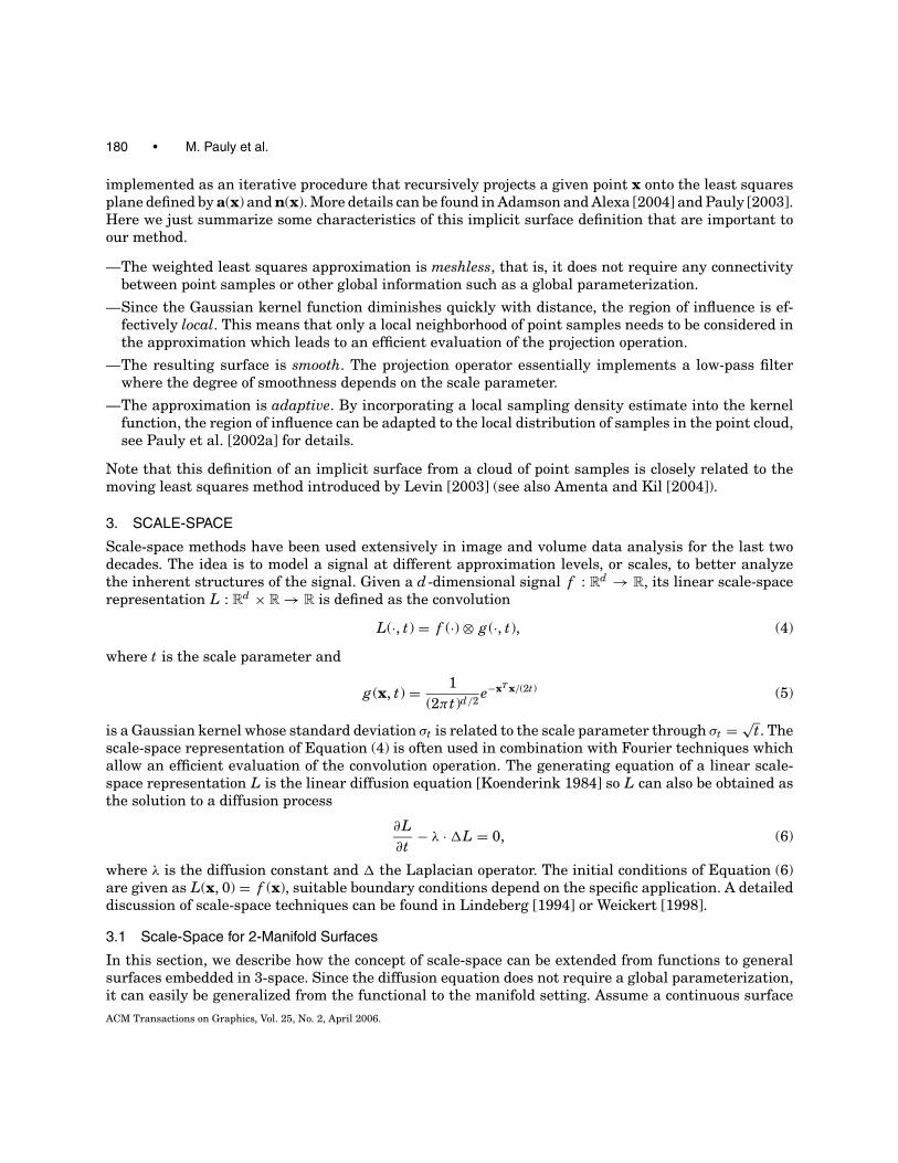
Fig. 1. Discrete multiscale representation. Left: 2D illustration, right: 3D surface model.

S is given. The surface diffusion equation defines a continuous set of evolving surfaces S(t) subjectto

∂x∂t

− λ�x = 0, (7)

where x ∈ S(t) is a point on the surface, t ∈ [0, ∞) ⊂ R denotes the time or scale parameter, and �x = κ ·nis the Laplace-Beltrami operator applied to the coordinate functions with κ the mean curvature andn the surface normal at x (see do Carmo [1976]). The initial condition to Equation (7) is given asS(0) = S. Equation (7) defines an evolving surface where each point on the surface moves in the directiondefined by the surface normal with a speed given by the mean curvature. This method, also known asmean curvature flow [Dziuk 1991], has been studied in the context of evolving interfaces [Sethian andOsher 1988] and surface fairing [Desbrun et al. 1999; Clarenz et al. 2000]. Note that this extension ofscale-space to 2-manifold surfaces does not have the properties of axiomatic scalespace theory such asnoncreation of maxima. Mean curvature flow can actually lead to an increase in curvature and evencreate singularities, for example, when applied to a dumbbell shape (see also Section 5.3).

4. DISCRETE MULTISCALE SURFACE REPRESENTATION

Given the definition of scale-space for manifold surfaces, we can now define our discrete multiscalesurface representation. The goal is to represent a given surface S by a discrete set of point cloudsP = {P0, . . . , Pk} where each of these point clouds defines an approximation to S at a different scale levelwith P0 as the smoothest approximation. Thus P can be understood as a discretization of Equation (7)both in space and in time (or scale), see Figure 1. To define adequate semantics for this discrete mul-tiscale surface representation, subsequent approximation levels need to be encoded relative to eachother in a meaningful way. This is done by means of a decomposition operator that encodes a detailedsurface as a normal displacement of its smooth approximation. As will be demonstrated, normal dis-placements ensure intuitive editing semantics and provide a compact representation of surface detail.While the decomposition operator defines the transition from detailed to smooth approximation, thereconstruction operator describes the inverse operation, that is, it adds detail to a smooth surface.

Formally, a discrete multiscale representation for point-sampled surfaces can be defined as follows.Let P = {p1, . . . , pn} be a point cloud representing a surface S and S(t) a continuous multiscale rep-resentation of S as defined by Equation (7). A discrete, point-based multiscale representation of S is asequence of point clouds P = {P0, . . . , Pk}, such that

—for all l ∈ {0, . . . , k−1}, there exists a tl ∈ [0, ∞) such that the surface represented by Pl approximatesSl = S(tl ) with tl > tl+1, where tk = 0 and Pk = P ,



—|Pl | = |P | = n for all l ∈ 0, . . . , k,

—for all pli ∈ Pl and all l ∈ {1, . . . , k}, there exists a pl−1

i ∈ Pl−1 such that

pli = pl−1

i + dl−1i · nl−1

i , (8)

where nl−1i is the surface normal at pl−1

i and dl−1i a scalar-valued detail coefficient.

Thus each sample pi ∈ P is represented by a point p0i ∈ P0 plus a sequence of normal displacement

offsets d0i , . . . , dk−1

i . To reconstruct the position of pli at a certain level, l the point p0

i is recursivelydisplaced in normal direction, that is,

pli = p0

i + d0i · n0

i + · · · + dl−1i · nl−1

i . (9)

Let D = {D0, . . . , Dk−1}, where Dl = {dl1, . . . , dl

n} is the set of detail coefficients at level l . The re-construction operator + : (P, D) → P can be defined by applying Equation (8) for each point of theargument point cloud, such that

Pl = Pl−1 + Dl−1. (10)

Then the reconstruction of a point cloud Pl can be written as

Pl = P0 +l−1∑

m=0

Dm, (11)

which directly corresponds to Equation (9). The inverse of the reconstruction operator is the decomposi-tion operator that determines the detail coefficients of the normal displacement offset between two pointclouds. The definition of a discrete multiscale representation implies that each sample point pi ∈ P isactive on all levels. The polygon p0

i , . . . , pki defines the normal trajectory of pi since each polygon edge

pli p

l+1i is aligned to the normal vector nl

i . At each level l , the point set Pl defines the model surface Sl atthe corresponding scale with level 0 the smoothest approximation. Note that no subsampling operatoris applied to the lower levels since unambiguous reconstruction of the normal trajectory requires thateach intermediate point pl

i is present.To build a discrete multiscale representation from a given point-sampled surface, we thus require a

smoothing operator to create successively smoother approximations of the input surface and a decom-position operator to encode subsequent levels in the hierarchy.

5. SMOOTHING OPERATOR

In Section 3, scale-space representations have been defined using either a convolution with a Gaussianor as the solution of a diffusion process. These equivalent definitions suggest two different approachesfor deriving smoothing operators for discrete surfaces. Traditionally, a discretization of the surfacediffusion equation has been used which leads to an iterative scheme for surface fairing (Section 5.1).Alternatively, one can exploit the low-pass filtering effect of the weighted least squares projection whichresembles the implementation of a Gaussian convolution filter (Section 5.2).

5.1 Surface Smoothing Based on Diffusion

For discrete surfaces, a variety of surface fairing methods have been introduced in recent years basedon a discretization of Equation (7) [Dziuk 1988; Taubin 1995; Desbrun et al. 1999; Pinkall and Polthier1993]. Special attention has to be given to a suitable discretization of the Laplacian as neither globalparameterization nor a regular sampling pattern are provided in the surface setting. Taubin [1995] pi-oneered these surface fairing methods and presented various approximate low-pass filters for triangle



meshes using different discrete approximations of the Laplacian. His approach aims at generalizingsignal processing techniques to manifold surfaces. For this purpose, he defines discrete geometric fre-quencies (see also Gross and Hubeli [2000] and Karni and Gotsman [2000]) as the eigenvectors ofthe Laplacian matrix which describes the discretization of the Laplacian as a weighted sum of adja-cent vertices. This discretization leads to the common iterative explicit Euler integration formula forapproximate Gaussian mesh smoothing

v′ = v + λ�v, (12)

where v′ is the new vertex position, and �v is some discrete approximation of the Laplacian at vertexv. Taubin demonstrates that this iterative scheme attenuates high frequencies while preserving lowfrequencies and thus implements approximate low-pass filter behavior.

This concept can be extended to point clouds by replacing the one-ring neighborhood relation with aspatial neighborhood relation, for example, the k-nearest neighbors (see Linsen and Prautzsch [2002] orPauly et al. [2002a] for a discussion of different point neighborhood relations). The degree of smoothnesscan be controlled by the parameter λ (see Equation (12)), the number m of iterations, and the size kof the local neighborhoods of the sample points. To improve the efficiency of the computations, localneighborhoods should be computed at the beginning of the smoothing operation and cached during theiteration. This also increases the stability of the smoothing filter since it prevents clustering effects dueto the tangential drift of sample points (see also Linsen [2001]).

A well known characteristic of iterative Laplacian smoothing is the slow convergence for low geo-metric frequencies. While high frequencies are attenuated quickly, a substantial number of iterationsis required to smooth out lower frequency detail. To alleviate this problem, Kobbelt et al. [1998] in-troduced multilevel fairing, using a complete v-cycle of alternating smoothing/subsampling, and up-sampling/smoothing steps. This scheme has been generalized to point clouds in Pauly et al. [2002b]where additionally a method for local volume preservation has been presented.

5.2 Surface Smoothing Based on Least Squares Filtering

An alternative approach for surface smoothing makes use of the low-pass filter characteristics of theleast squares projection operator (see Section 2). A smooth approximation of a given point set P can beobtained by simply projecting all points of P onto the implicit surface defined by P . By adjusting thekernel width h in φx (see Equation (3)), different degrees of smoothness can be obtained. In fact, h canbe understood as a continuous scale parameter in the sense of the scale-space representation describedpreviously. This means that the least squares projection replaces the fairing operator for creating thescale-space approximation of a given surface S.

One difficulty with using a large kernel width in the projection is that large subsets of the pointcloud have to considered in the least squares optimization which quickly leads to excessive com-putation times. A substantial improvement in performance can be obtained by integrating a deci-mation operator. Since large kernels imply that each individual point contributes less to the opti-mization, clusters of points can be replaced by a single point without significant loss of accuracy(see also Alexa et al. [2001]). Thus by first decimating the point cloud, the projection operator canbe evaluated much more efficiently. For decimation we use the hierarchical clustering method de-scribed in Pauly et al. [2002a] that adaptively separates a given point cloud into clusters, each ofwhich is replaced by its centroid. This averaging step already implements a low pass-filter, thusthe method is not prone to resampling artifacts such as surface aliasing. Starting with the originalpoint cloud P = Pk , clustering builds a hierarchy P → Qk−1 → · · · → Q0 of point clouds withsuccessively lower sampling density. Note that, even though a decimation is applied, the projectedpoint clouds Pl = �Ql (P ), l = 0, . . . , k − 1 still have the same number of sample points as P . The



decimation only affects the intermediate point clouds Ql that define the base surface of the projectionoperator.

A crucial question remains: What is the appropriate decimation rate for a certain kernel width?The qualitative argument given indicates that the larger the kernel width, that is, the smoother theresulting surface should be, the can the decimation rate can be without losing too much accuracy.However, a precise quantitative relation is difficult to formulate. Thus a different approach is chosenthat controls the degree of smoothness using the sampling resolution. The kernel width is coupled to thelocal sampling density, for example, as a constant times the local sample spacing [Pauly et al. 2002a].Thus instead of specifying a discrete set of kernel widths, the discrete scale-space approximation isdefined by a set of sampling resolutions nk , . . . , n0 such that nk = n = |Pk|, |Ql | = nl , and nl > nl−1

for 1 ≤ l ≤ k. A suitable choice for the nl is a geometric series, that is, nl−1 = �γ l · n�, where γ ∈ (0, 1)is the decimation factor. This approach defines a logarithmic number of discrete scale-space levelsin the number of input samples n and corresponds to pyramid algorithms used in multiresolutionmethods [Zorin et al. 1997].

5.3 Discussion

Smoothing operators based on diffusion or the least squares projection operation are only approxi-mate low-pass filters. Since no global, distortion-free parameterization exists for manifolds in general,applying these filters can lead to deformations such as volume shrinkage. Another issue is that theprojection tends to become unstable for very large filter widths or very low sampling densities due tosuccessive decimation. For example, consider an approximation of a sphere where the kernel width hasbeen chosen so large that all points on the sphere have about the same weight. It is not clear what thecorrect least squares plane for such a configuration should be. For practical purposes, however, theseproblems are less of an issue since the kernel function for the smoothest level in the decomposition istypically not in this region of instability. Note that the use of decimation for the projection essentiallyfollows the same motivation as the multilevel fairing methods of Kobbelt et al. [1998] and Pauly et al.[2002b] as it avoids excessive computation times for the attenuation of low frequencies.

6. DECOMPOSITION OPERATOR

Suppose a discrete scale-space approximation Q = {Q0, . . . , Qk} of a surface S has been computed usinggeometric low-pass filtering as described in Section 5. To encode Ql with respect to Ql−1, the detailcoefficients Dl−1 need to be computed. In general, however, it is not possible to find for each ql

i ∈ Ql a

corresponding sample ql−1i ∈ Ql−1 such that the displacement is in normal direction, that is,

(ql−1

i − qli

) · nl−1i = 0. (13)

Thus to obtain a discrete multiscale representation P = {P0, . . . , Pk} for the surface S, the surfacesrepresented by the Ql need to be resampled to fulfill the normal displacement criterion. We will de-scribe two alternatives to compute the sequence D of sets of detail coefficients and the sequence P fromthe discrete scale-space approximation Q. Suppose two subsequent levels Sl−1 and Sl are given, repre-sented by two point clouds Ql−1 and Ql , respectively. The goal is to find two point clouds Pl−1 and Pl ,approximating the surfaces Sl−1 and Sl , and a set of detail coefficients Dl−1 such that Pl = Pl−1+ Dl−1.

6.1 Bottom-Up Encoding by Ray-Shooting

One approach is to shoot a ray from each ql−1i ∈ Ql−1 in normal direction and find the intersection point

rli ∈ Sl with the surface Sl . Then the corresponding detail coefficient is given as

d j−1i = ∥∥rl

i − ql−1i

∥∥. (14)



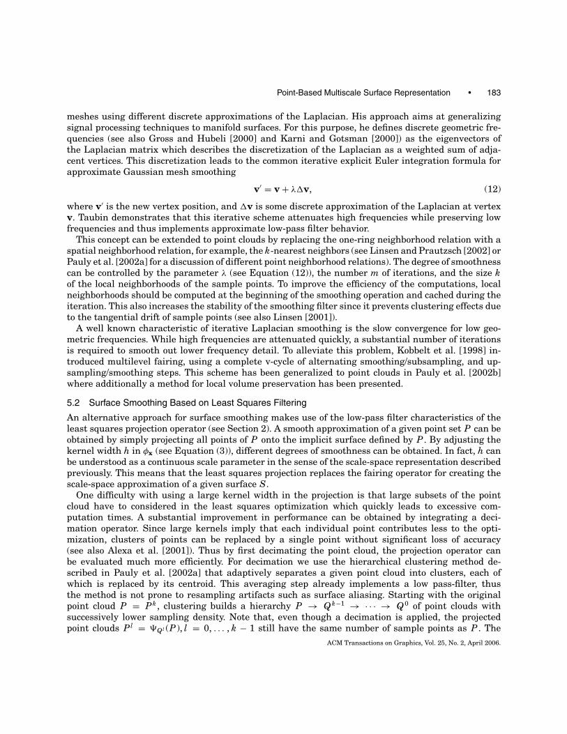
Fig. 2. Multiscale encoding: The point cloud in the middle is obtained as a normal displacement of the point cloud on the left.

The right image shows the corresponding detail coefficients, where blue indicates maximum negative displacement and red

maximum positive displacement for outward pointing normals.

Furthermore,

Pl−1 = Ql−1 (15)

and

Pl = {rl

i |i = 1, . . . , n}. (16)

This means that the point cloud Ql−1 representing the smooth surface Sl−1 is left unchanged, while thepoint cloud Ql representing the detailed surface Sl is re-sampled to fulfill the normal displacement con-dition. This method of ray-shooting has been applied successfully in previous mesh-based approaches,for example, in Guskov et al. [2000] to build a normal mesh hierarchy. An algorithm for intersecting aray with the implicit surface defined in Section 2 has been introduced in Adamson and Alexa [2003].In this method, a point on the ray is iteratively projected onto the surface until it converges to a pointboth on the ray and the surface.

6.2 Top-Down Encoding by Projection

The second alternative would be to start with a point qli ∈ Ql and project it onto the surface Sl−1. Thus

a point rl−1i = �Ql−1 (ql

i ) ∈ Sl−1 is obtained, where �Ql−1 is the least squares projection operator with

respect to the point cloud Ql−1. This yields

d j−1i = ∥∥ql

i − rl−1i

∥∥. (17)

Furthermore,

Pl−1 = {rl−1

i |i = 1, . . . , n}

(18)

and

Pl = Ql . (19)

Here the smooth surface is resampled, while the detailed point cloud remains unaltered.Figure 2 illustrates the encoding of two subsequent levels. Note that the projection operator as defined

in Section 2 is not strictly orthogonal, that is, the direction of projection does not coincide exactly withthe surface normal. As described in Adamson and Alexa [2004], a strictly orthogonal projection canbe obtained by restricting the projection direction to the gradient of the implicit function f . Thismethod is computationally more involved, however. In practice, the simple projection procedure leadsto satisfactory results since the deviation from the true normal is negligible when projecting onto the



Fig. 3. Linear blend between two subsequent levels of a multiscale representation.

low-pass filtered surface Sl−1. Compared with ray shooting, the top-down is in general more stablesince the surface Sl−1 is a smooth approximation of the surface Sl . Thus resampling Sl−1 will lead tofewer sampling artifacts such as aliasing, s compared to resampling of Sl .

6.3 Continuous Representation

Note that, even though the sequence of point clouds P = {P0, . . . , Pk} defines a discrete sample alongthe scale axis, a continuous scale-space approximation can be obtained by interpolation. For example,a linear blend between two successive levels Pl−1 and Pl can be defined as

Pl (α) = Pl−1 + α · Dl−1, (20)

where α ∈ [0, 1] is the blending parameter, Pl (0) = Pl−1, and Pl (1) = Pl . This corresponds to a linearblend between each individual sample described as

pli (α) = pl−1

i + α · dl−1i · nl−1

i . (21)

Figure 3 illustrates a linear blend between two subsequent levels.

7. INTEGRATED SMOOTHING AND DECOMPOSITION OPERATOR

Recall that the construction of a multiscale representation requires an alternating series of two basicoperations: A low-pass filter (smoothing operator) to obtain a smoother approximation of a given surfaceand an encoding step (decomposition operator) to establish the connection between two successivelevels. We have shown how the latter can be implemented using the least squares projection methodand, similarly, in Section 5.2, it has been demonstrated how the same projection can be used for surfacesmoothing. Thus we can combine the low-pass filter and encoding steps into a single operator.

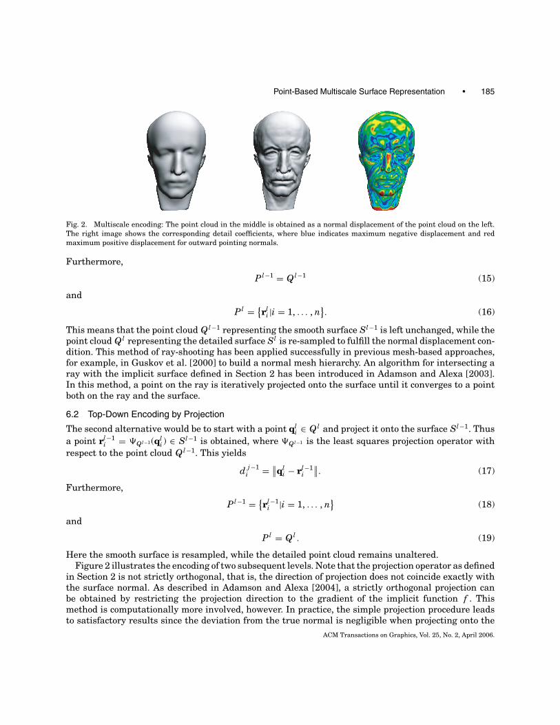
The complete construction of the multiscale representation then proceeds as follows (see Figure 4).We start with the original point cloud Pk = P and apply the decimation operator to obtain Qk−1. Usingan appropriate Gaussian kernel, we then project all points of Pk onto the implicit surface defined byQk−1. This yields a low-pass filtered version of Pk , the point cloud Pk−1. We then obtain the detailcoefficients Dk−1 by computing the point-wise Euclidean distance as in Equation (17). Now we caniterate this procedure of decimation and projection until the desired level of smoothness is achieved.

The cost for the construction of the multiscale representation is dominated by the least squaresprojections. In comparison, the decimation typically requires less than 5% of the total computationtime. Since a single projection is applied for low-pass filtering and decomposition, the total numberof projections is k · n, where k is the number of discrete scale levels and n = |P | is the number ofpoint samples. Note that the successive decimation of the point cloud does not reduce the number ofrequired projections, since each point cloud Pl has the same number of sample points. Instead, theefficiency of the projection is greatly increased for higher smoothness levels since fewer samples haveto be considered in the least squares optimization.



Fig. 4. Building a discrete multiscale representation.

Still, since the full projection is rather costly, the computational effort for the construction of a mul-tiscale representation is quite significant. However, once this representation is built, reconstruction ofindividual levels is very efficient since it only requires the points to be displaced in the normal directionaccording to the detail coefficients.

As previously mentioned above, the multiscale point cloud representation is a discrete sample of thecontinuous representation both in space and in scale. In this context, the low-pass filter determines thesampling in the scale dimension by controlling the smoothness of the approximation. The decompositionalgorithm, on the other hand, needs to find the base points on the smoother level to define the detailcoefficients and thus determines the sampling in the spatial dimension.

8. RESULTS AND APPLICATIONS

This section presents various applications for the multiscale representation. The focus is on surfaceediting and filtering, other applications will be addressed in the future work section.

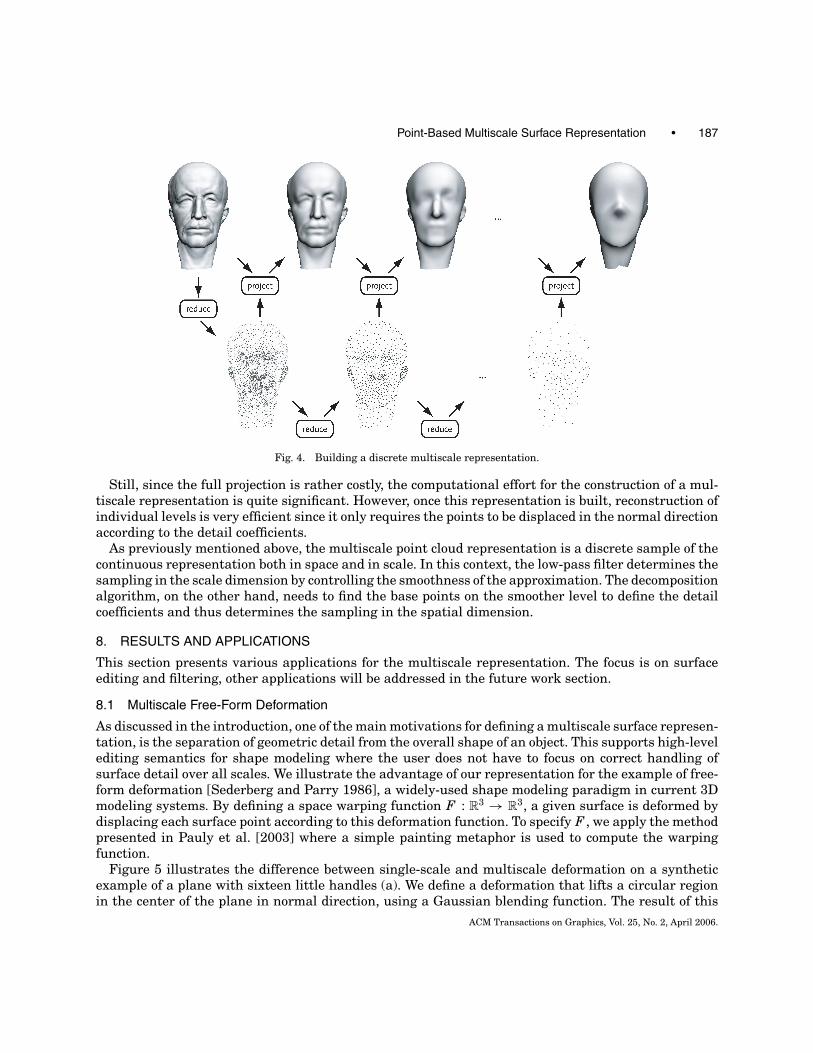
8.1 Multiscale Free-Form Deformation

As discussed in the introduction, one of the main motivations for defining a multiscale surface represen-tation, is the separation of geometric detail from the overall shape of an object. This supports high-levelediting semantics for shape modeling where the user does not have to focus on correct handling ofsurface detail over all scales. We illustrate the advantage of our representation for the example of free-form deformation [Sederberg and Parry 1986], a widely-used shape modeling paradigm in current 3Dmodeling systems. By defining a space warping function F : R

3 → R3, a given surface is deformed by

displacing each surface point according to this deformation function. To specify F , we apply the methodpresented in Pauly et al. [2003] where a simple painting metaphor is used to compute the warpingfunction.

Figure 5 illustrates the difference between single-scale and multiscale deformation on a syntheticexample of a plane with sixteen little handles (a). We define a deformation that lifts a circular regionin the center of the plane in normal direction, using a Gaussian blending function. The result of this



Fig. 5. Multiscale vs. single-scale modeling. (a) original surface, (b) smooth base domain, (c) deformed base domain, (d) single-

scale deformation, (e) multiscale deformation.

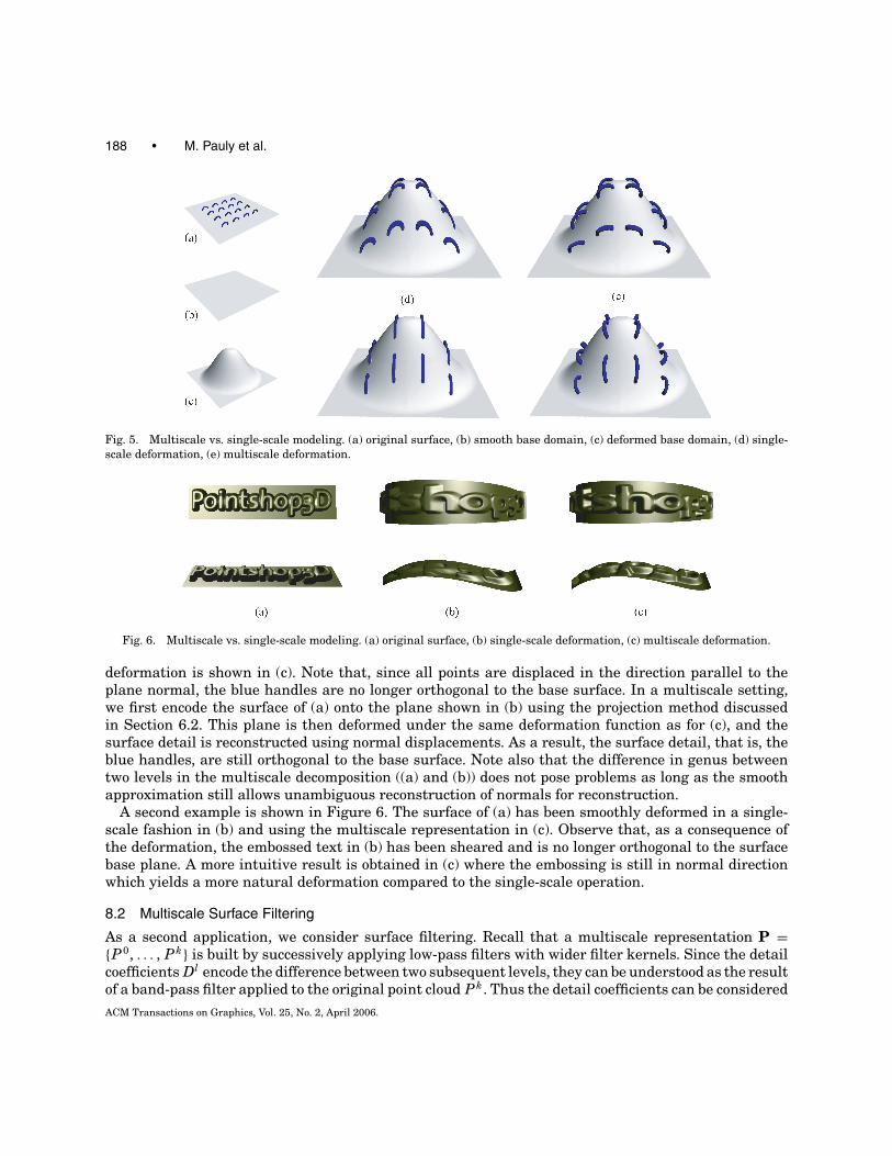
Fig. 6. Multiscale vs. single-scale modeling. (a) original surface, (b) single-scale deformation, (c) multiscale deformation.

deformation is shown in (c). Note that, since all points are displaced in the direction parallel to theplane normal, the blue handles are no longer orthogonal to the base surface. In a multiscale setting,we first encode the surface of (a) onto the plane shown in (b) using the projection method discussedin Section 6.2. This plane is then deformed under the same deformation function as for (c), and thesurface detail is reconstructed using normal displacements. As a result, the surface detail, that is, theblue handles, are still orthogonal to the base surface. Note also that the difference in genus betweentwo levels in the multiscale decomposition ((a) and (b)) does not pose problems as long as the smoothapproximation still allows unambiguous reconstruction of normals for reconstruction.

A second example is shown in Figure 6. The surface of (a) has been smoothly deformed in a single-scale fashion in (b) and using the multiscale representation in (c). Observe that, as a consequence ofthe deformation, the embossed text in (b) has been sheared and is no longer orthogonal to the surfacebase plane. A more intuitive result is obtained in (c) where the embossing is still in normal directionwhich yields a more natural deformation compared to the single-scale operation.

8.2 Multiscale Surface Filtering

As a second application, we consider surface filtering. Recall that a multiscale representation P ={P0, . . . , Pk} is built by successively applying low-pass filters with wider filter kernels. Since the detailcoefficients Dl encode the difference between two subsequent levels, they can be understood as the resultof a band-pass filter applied to the original point cloud Pk . Thus the detail coefficients can be considered



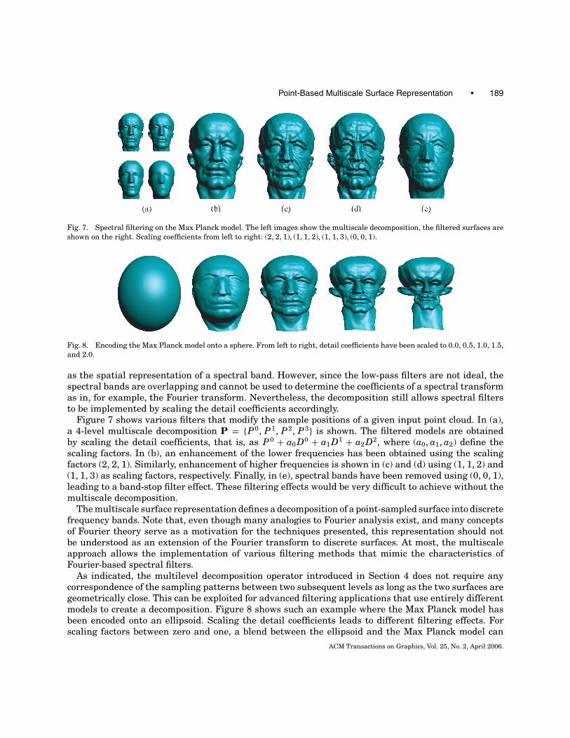
Fig. 7. Spectral filtering on the Max Planck model. The left images show the multiscale decomposition, the filtered surfaces are

shown on the right. Scaling coefficients from left to right: (2, 2, 1), (1, 1, 2), (1, 1, 3), (0, 0, 1).

Fig. 8. Encoding the Max Planck model onto a sphere. From left to right, detail coefficients have been scaled to 0.0, 0.5, 1.0, 1.5,

and 2.0.

as the spatial representation of a spectral band. However, since the low-pass filters are not ideal, thespectral bands are overlapping and cannot be used to determine the coefficients of a spectral transformas in, for example, the Fourier transform. Nevertheless, the decomposition still allows spectral filtersto be implemented by scaling the detail coefficients accordingly.

Figure 7 shows various filters that modify the sample positions of a given input point cloud. In (a),a 4-level multiscale decomposition P = {P0, P1, P2, P3} is shown. The filtered models are obtainedby scaling the detail coefficients, that is, as P0 + a0 D0 + a1 D1 + a2 D2, where (a0, a1, a2) define thescaling factors. In (b), an enhancement of the lower frequencies has been obtained using the scalingfactors (2, 2, 1). Similarly, enhancement of higher frequencies is shown in (c) and (d) using (1, 1, 2) and(1, 1, 3) as scaling factors, respectively. Finally, in (e), spectral bands have been removed using (0, 0, 1),leading to a band-stop filter effect. These filtering effects would be very difficult to achieve without themultiscale decomposition.

The multiscale surface representation defines a decomposition of a point-sampled surface into discretefrequency bands. Note that, even though many analogies to Fourier analysis exist, and many conceptsof Fourier theory serve as a motivation for the techniques presented, this representation should notbe understood as an extension of the Fourier transform to discrete surfaces. At most, the multiscaleapproach allows the implementation of various filtering methods that mimic the characteristics ofFourier-based spectral filters.

As indicated, the multilevel decomposition operator introduced in Section 4 does not require anycorrespondence of the sampling patterns between two subsequent levels as long as the two surfaces aregeometrically close. This can be exploited for advanced filtering applications that use entirely differentmodels to create a decomposition. Figure 8 shows such an example where the Max Planck model hasbeen encoded onto an ellipsoid. Scaling the detail coefficients leads to different filtering effects. Forscaling factors between zero and one, a blend between the ellipsoid and the Max Planck model can



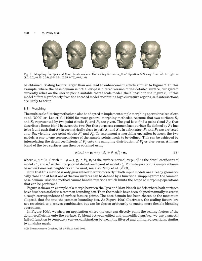
Fig. 9. Morphing the Igea and Max Planck models. The scaling factors (α, β) of Equation (22) vary from left to right as

(1.0, 0.0), (0.75, 0.25), (0.5, 0.5), (0.25, 0.75), (0.0, 1.0).

be obtained. Scaling factors larger than one lead to enhancement effects similar to Figure 7. In thisexample, where the base domain is not a low-pass filtered version of the detailed surface, our systemcurrently relies on the user to pick a suitable coarse scale model (the ellipsoid in the Figure 8). If thismodel differs significantly from the encoded model or contains high curvature regions, self-intersectionsare likely to occur.

8.3 Morphing

The multiscale filtering method can also be adapted to implement simple morphing operations (see Alexaet al. [2000] or Lee et al. [1999] for more general morphing methods). Assume that two surfaces S1

and S2 represented by two point clouds P1 and P2 are given. The goal is to find a point cloud PM thatdescribes a linear blend between the two. For this purpose a common base surface SB defined by PB hasto be found such that SB is geometrically close to both S1 and S2. In a first step, P1 and P2 are projectedonto SB, yielding two point clouds P ′

1 and P ′2. To implement a morphing operation between the two

models, a one-to-one correspondence of the sample points needs to be defined. This can be achieved byinterpolating the detail coefficients of P ′

2 onto the sampling distribution of P ′1 or vice versa. A linear

blend of the two surfaces can then be obtained using

pi(α, β) = pi + (α · d1

i + β · d2i

) · ni, (22)

where α, β ∈ [0, 1] with α + β = 1, pi ∈ P ′1, ni is the surface normal at pi, d1

i is the detail coefficient of

model P ′1, and d2

i is the interpolated detail coefficient of model P ′2. For interpolation, a simple scheme

based on k-nearest neighbors can be used, see also Pauly et al. [2003].Note that this method is only guaranteed to work correctly if both input models are already geometri-

cally close and at least one of the two surfaces can be defined by a functional mapping from the commonbase domain. Also the method cannot handle rotations which limits the scope of morphing operationsthat can be performed.

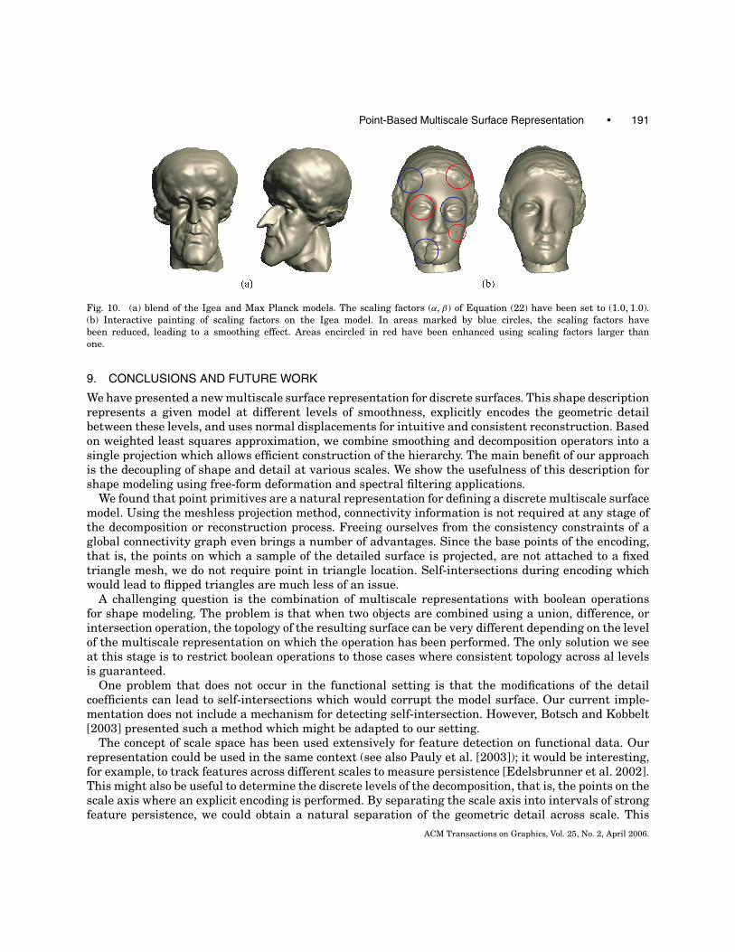
Figure 9 shows an example of a morph between the Igea and Max Planck models where both surfaceshave first been scaled to a common bounding box. Then the models have been aligned manually to createa rough correspondence of surface feature points. The base domain has been chosen as the maximumellipsoid that fits into the common bounding box. As Figure 10(a) illustrates, the scaling factors arenot restricted to a convex combination but can be chosen arbitrarily to enable more flexible blendingoperations.

In Figure 10(b), we show an application where the user can directly paint the scaling factors of thedetail coefficients onto the surface. To blend between edited and unmodified surface, we use a smoothfall-off function to compute a convex combination between the filtered and unfiltered positions, similarto an alpha mask.



Fig. 10. (a) blend of the Igea and Max Planck models. The scaling factors (α, β) of Equation (22) have been set to (1.0, 1.0).

(b) Interactive painting of scaling factors on the Igea model. In areas marked by blue circles, the scaling factors have

been reduced, leading to a smoothing effect. Areas encircled in red have been enhanced using scaling factors larger than

one.

9. CONCLUSIONS AND FUTURE WORK

We have presented a new multiscale surface representation for discrete surfaces. This shape descriptionrepresents a given model at different levels of smoothness, explicitly encodes the geometric detailbetween these levels, and uses normal displacements for intuitive and consistent reconstruction. Basedon weighted least squares approximation, we combine smoothing and decomposition operators into asingle projection which allows efficient construction of the hierarchy. The main benefit of our approachis the decoupling of shape and detail at various scales. We show the usefulness of this description forshape modeling using free-form deformation and spectral filtering applications.

We found that point primitives are a natural representation for defining a discrete multiscale surfacemodel. Using the meshless projection method, connectivity information is not required at any stage ofthe decomposition or reconstruction process. Freeing ourselves from the consistency constraints of aglobal connectivity graph even brings a number of advantages. Since the base points of the encoding,that is, the points on which a sample of the detailed surface is projected, are not attached to a fixedtriangle mesh, we do not require point in triangle location. Self-intersections during encoding whichwould lead to flipped triangles are much less of an issue.

A challenging question is the combination of multiscale representations with boolean operationsfor shape modeling. The problem is that when two objects are combined using a union, difference, orintersection operation, the topology of the resulting surface can be very different depending on the levelof the multiscale representation on which the operation has been performed. The only solution we seeat this stage is to restrict boolean operations to those cases where consistent topology across al levelsis guaranteed.

One problem that does not occur in the functional setting is that the modifications of the detailcoefficients can lead to self-intersections which would corrupt the model surface. Our current imple-mentation does not include a mechanism for detecting self-intersection. However, Botsch and Kobbelt[2003] presented such a method which might be adapted to our setting.

The concept of scale space has been used extensively for feature detection on functional data. Ourrepresentation could be used in the same context (see also Pauly et al. [2003]); it would be interesting,for example, to track features across different scales to measure persistence [Edelsbrunner et al. 2002].This might also be useful to determine the discrete levels of the decomposition, that is, the points on thescale axis where an explicit encoding is performed. By separating the scale axis into intervals of strongfeature persistence, we could obtain a natural separation of the geometric detail across scale. This



means that, whenever a large number of features vanishes or disappears, a new level in the hierarchywould be inserted.

Since the least squares filter with radially symmetric Gaussian kernel is isotropic, features are notpreserved, and the directional aspect of features is ignored. It would be interesting to extend our schemeusing anisotropic smoothing operators, for example, the bilateral filters presented in Fleishman et al.[2003] and Jones et al. [2003].

REFERENCES

ADAMSON, A. AND ALEXA, M. 2003. Approximating and intersecting surfaces from points. In Proceedings of the Eurograph-ics/ACM SIGGRAPH Symposium on Geometry Processing. Eurographics Association, 230–239.

ADAMSON, A. AND ALEXA, M. 2004. On normals and projection operators for surfaces defined by point sets. In Proceedings ofthe Eurographics Symposium on Point-Based Graphics. Eurographics Association, 150–155.

ALEXA, M., BEHR, J., COHEN-OR, D., FLEISHMAN, S., LEVIN, D., AND SILVA, C. T. 2001. Point set surfaces. In Proceedings of theConference on Visualization. IEEE Computer Society Press, 21–28.

ALEXA, M., COHEN-OR, D., AND LEVIN, D. 2000. As-rigid-as-possible shape interpolation. In Proceedings of the 27th AnnualConference on Computer Graphics and Interactive Techniques. ACM Press, 157–164.

AMENTA, N. AND KIL, Y. J. 2004. Defining point-set surfaces. ACM Trans. Graph. 23, 3, 264–270.

BOTSCH, M. AND KOBBELT, L. 2003. Multiresolution surface representation based on displacement volumes. Comput. Graph.Forum 22, 483–491.

BOTSCH, M. AND KOBBELT, L. 2004. An intuitive framework for real-time freeform modeling. ACM Trans. Graph. 23, 3, 630–634.

CARLSON, M., MUCHA, P. J., VAN HORN, III, R. B., AND TURK, G. 2002. Melting and flowing. In Proceedings of the ACMSIGGRAPH/Eurographics Symposium on Computer Animation. ACM Press, 167–174.

CLARENZ, U., DIEWALD, U., AND RUMPF, M. 2000. Anisotropic geometric diffusion in surface processing. In Proceedings of theConference on Visualization. IEEE Computer Society Press, 397–405.

DESBRUN, M., MEYER, M., SCHRODER, P., AND BARR, A. H. 1999. Implicit fairing of irregular meshes using diffusion and curvature

flow. In Proceedings of the 26th Annual Conference on Computer Graphics and Interactive Techniques. ACM Press, 317–324.

DO CARMO, M. P. 1976. Differential Geometry of Curves and Surfaces. Prentice Hall.

DZIUK, G. 1988. Finite elements for the beltrami operator on arbitrary surfaces. Partial differential equations and calculus

of variations. S. Hildebrandt, R. Leis, Eds. Lecture Notes in Mathematics vol. 1357, 142–155.

DZIUK, G. 1991. An algorithm for evolutionary surfaces. Numerische Mathematik 58, 6, 603–611.

ECK, M., DEROSE, T., DUCHAMP, T., HOPPE, H., LOUNSBERY, M., AND STUETZLE, W. 1995. Multiresolution analysis of arbitrary

meshes. In Proceedings of the 22nd Annual Conference on Computer Graphics and Interactive Techniques. ACM Press, 173–

182.

EDELSBRUNNER, H., LETSCHER, D., AND ZOMORODIAN, A. 2002. Topological persistence and simplification. In Proceedings of the41st IEEE Symposium on the Foundations of Computer Science. 454–463.

FELDMAN, B. E., O’BRIEN, J. F., AND ARIKAN, O. 2003. Animating suspended particle explosions. ACM Trans. Graph. 22, 3,

708–715.

FLEISHMAN, S., COHEN-OR, D., ALEXA, M., AND SILVA, C. T. 2003. Progressive point set surfaces. ACM Trans. Graph. 22, 4,

997–1011.

FLEISHMAN, S., DRORI, I., AND COHEN-OR, D. 2003. Bilateral mesh denoising. ACM Trans. Graph. 22, 3, 950–953.

GROSS, M. AND HUBELI, A. 2000. Eigenmeshes. Tech. rep., Department of Computer Science, ETH Zurich.

GUSKOV, I., SWELDENS, W., AND SCHRODER, P. 1999. Multiresolution signal processing for meshes. In Proceedings of the 26thAnnual Conference on Computer Graphics and Interactive Techniques. ACM Press, 325–334.

GUSKOV, I., VIDIMCE, K., SWELDENS, W., AND SCHRODER, P. 2000. Normal meshes. In Proceedings of the 27th Annual Conferenceon Computer Graphics and Interactive Techniques. ACM Press, 95–102.

HUBELI, A. AND GROSS, M. 2001. Multiresolution feature extraction from unstructured meshes. In Proceedings of the Conferenceon Visualization. IEEE Computer Society Press.

JONES, T. R., DURAND, F., AND DESBRUN, M. 2003. Non-iterative, feature-preserving mesh smoothing. ACM Trans. Graph. 22, 3,

943–949.

KALAIAH, A. AND VARSHNEY, A. 2003. Statistical point geometry. In Proceedings of the Eurographics/ACM SIGGRAPH Sympo-sium on Geometry Processing. Eurographics Association, 107–115.



KARNI, Z. AND GOTSMAN, C. 2000. Spectral compression of mesh geometry. In Proceedings of the 27th Annual Conference onComputer Graphics and Interactive Techniques. ACM Press, 279–286.

KHODAKOVSKY, A., SCHRODER, P., AND SWELDENS, W. 2000. Progressive geometry compression. In Proceedings of the 27th AnnualConference on Computer Graphics and Interactive Techniques. ACM Press, 271–278.

KOBBELT, L., CAMPAGNA, S., VORSATZ, J., AND SEIDEL, H.-P. 1998. Interactive multi-resolution modeling on arbitrary meshes. In

Proceedings of the 25th Annual Conference on Computer Graphics and Interactive Techniques. ACM Press, 105–114.

KOBBELT, L., VORSATZ, J., AND SEIDEL, H.-P. 1999. Multiresolution hierarchies on unstructured triangle meshes. Computat.Geometry J. Theory Appl., 5–24.

KOENDERINK, J. J. 1984. The structure of images. Biological Cybernetics 50, 363–370.

LEE, A. W. F., DOBKIN, D., SWELDENS, W., AND SCHRODER, P. 1999. Multiresolution mesh morphing. In Proceedings of the 26thAnnual Conference on Computer Graphics and Interactive Techniques. ACM Press, 343–350.

LEVIN, D. 2003. Mesh-independent surface interpolation. In Geometric Modeling for Scientific Visualization. Springer-Verlag,

37–50.

LEVOY, M. AND WHITTED, T. 1985. The use of points as display primitives. Tech. rep., Department of Computer Science, University

of North Carolina at Chappel Hill.

LINDEBERG, T. 1994. Scale-Space Theory In Computer Vision. Kluwer Academic Publishers.

LINSEN, L. 2001. Point cloud representation. Tech. rep., Faculty of Computer Science, University of Karlsruhe.

LINSEN, L. AND PRAUTZSCH, H. 2002. Fan clouds—an alternative to meshes. In Proceedings of Dagstuhl Seminar on TheoreticalFoundations of Computer Vision—Geometry, Morphology, and Computational Imaging.

MULLER, M., KEISER, R., NEALEN, A., PAULY, M., GROSS, M., AND ALEXA, M. 2004. Point based animation of elastic, plastic and

melting objects. In Proceedings of the ACM SIGGRAPH/Eurographics Symposium on Computer Animation (SCA ’04). ACM

Press, 141–151.

PAULY, M. 2003. Point primitives for interactive modeling and processing of 3d geometry. Ph.D. thesis, Computer Science

Department, ETH Zurich.

PAULY, M., GROSS, M., AND KOBBELT, L. P. 2002a. Efficient simplification of point-sampled surfaces. In Proceedings of theConference on Visualization. 163–170.

PAULY, M., KEISER, R., ADAMS, B., DUTRE, P., GROSS, M., AND GUIBAS, L. J. 2005. Meshless animation of fracturing solids. ACMTrans. Graph. 24, 3, 957–964.

PAULY, M., KEISER, R., AND GROSS, M. 2003. Multi-scale feature extraction on point-sampled surfaces. In Comput. Graph. Forum.

22, 281–289.

PAULY, M., KEISER, R., KOBBELT, L. P., AND GROSS, M. 2003. Shape modeling with point-sampled geometry. In ACM Trans. Graph.22, 641–650.

PAULY, M., KOBBELT, L., AND GROSS, M. 2002b. Multiresolution modeling of point-sampled geometry. Tech. rep., Department of

Computer Science, ETH Zurich.

PINKALL, U. AND POLTHIER, K. 1993. Computing discrete minimal surfaces and their conjugates. Experim. Math. 2, 1, 15–36.

ROSSIGNAC, J. AND BORREL, P. 1993. Multi-resolution 3d approximations for rendering. Model. Comput. Graph., 455–465.

SEDERBERG, T. W. AND PARRY, S. R. 1986. Free-form deformation of solid geometric models. In Proceedings of the 13th AnnualConference on Computer Graphics and Interactive Techniques. ACM Press, 151–160.

SETHIAN, J. A. AND OSHER, S. 1988. Fronts propagating with curvature-dependent speed: Algorithms based on hamilton-jacobi

formulations. J. Computat. Physics 79, 12–49.

TAUBIN, G. 1995. A signal processing approach to fair surface design. In Proceedings of the 22nd Annual Conference onComputer Graphics and Interactive Techniques. ACM Press, 351–358.

WEICKERT, J. 1998. Anisotropic Diffusion in Image Processing. Teubner-Verlag.

ZORIN, D., SCHRODER, P., AND SWELDENS, W. 1997. Interactive multiresolution mesh editing. In Proceedings of the 24th AnnualConference on Computer Graphics and Interactive Techniques. ACM Press, 259–268.

ZWICKER, M., PAULY, M., KNOLL, O., AND GROSS, M. 2002. Pointshop 3d: an interactive system for point-based surface editing. In

Proceedings of the 29th Annual Conference on Computer Graphics and Interactive Techniques. ACM Press, 322–329.

Received October 2003; revised June 2004; accepted September 2005


point-based multiscale surface...

Documents