Spectral Segmentation with Multiscale Graph Decomposition

Timothee Cour1 Florence Benezit2 Jianbo Shi31,3Computer and Information Science2Applied Mathematics Department

University of Pennsylvania Ecole PolytechniquePhiladelphia, PA 19104 91128 Palaiseau Cedex, FRANCE

timothee@seas.upenn.edu florence.benezit@polytechnique.org

Abstract

We present a multiscale spectral image segmentation al-gorithm. In contrast to most multiscale image processing,this algorithm works on multiple scales of the image in par-allel, without iteration, to capture both coarse and fine leveldetails. The algorithm is computationally efficient, allowingto segment large images. We use the Normalized Cut graphpartitioning framework of image segmentation. We con-struct a graph encoding pairwise pixel affinity, and parti-tion the graph for image segmentation. We demonstrate thatlarge image graphs can be compressed into multiple scalescapturing image structure at increasingly large neighbor-hood. We show that the decomposition of the image seg-mentation graph into different scales can be determined byecological statistics on the image grouping cues. Our seg-mentation algorithm works simultaneously across the graphscales, with an inter-scale constraint to ensure communi-cation and consistency between the segmentations at eachscale. As the results show, we incorporate long-range con-nections with linear-time complexity, providing high-qualitysegmentations efficiently. Images that previously could notbe processed because of their size have been accurately seg-mented thanks to this method.

1. Introduction

There are two things you could do to make image seg-mentation difficult: 1) camouflage the object by making itsboundary edges faint, and 2) increase clutter by makingbackground edges highly contrasting, particularly those intextured regions. In fact, such situations arise often in natu-ral images, as animals have often evolved to blend into theirenvironment.

Several recent works have demonstrated that multiscaleimage segmentation can produce impressive segmentationresults under these difficult conditions. Sharon, et. al. [9]

uses an algebraic multi-grid method for solving the normal-ized cut criterion efficiently, and uses recursive graph coars-ening to produce irregular pyramid encoding region basedgrouping cues. Yu [11] constructs a multiple level graph en-coding edge cues at different image scales, and optimizesthe average Ncut cost across all graph levels. Zhu et. al. [1]explicitly controls the Markov chain transitions in the spaceof graph partitions by splitting, merging and re-groupingsegmentation graph nodes.

We argue that there are in fact three orthogonal issuesin multiscale image segmentation: 1)multiscale signal pro-cessingto enhance faint contours [6, 2]; 2)image regionsimilarity cuesat multiple scales provides texture/shapecues for larger regions; 3)propagationof local groupingcues across multiple ranges of spatial connections allows usto detect coherent regions with faint boundary.

Sharon [9], Zhu [1]’s approaches focus on the last two is-sues, and Yu [11] focuses on the first and third. The primarymotivation underlying all these approaches is that local in-formation propagates faster with long range connectionsacross image regions, and computation converges fasterboth in graph partitioning and MRF probabilistic formu-lation. Both Sharon and Zhu advocateddata driven adap-tive coarsening of an image region/segmentation graph asan essential step in multiscale segmentation. This conclu-sion is partly justified by the failure of most multiscale seg-mentation algorithms [8, 7, 4] which use simple geometriccoarsening of images: typically fine level details along ob-ject boundaries are lost due to coarsening error.

We focus on the third issue of multiscale propagation ofgrouping cuesin isolation. We show that simple geomet-ric coarsening of the image region/segmentation graphcanwork for multiscale segmentation. The key principle is thatsegmentation across different spatial scales should be pro-cessed inparallel. We specify the constraint that segmen-tation must be self-consistent across the scales. This con-straint forces the system to seek an “average” segmentationacross all scales. We show our multiscale segmentation al-gorithm can precisely segment objects with both fine and

coarse level object details.The advantage of graphs with long connections comes

with a great computational cost. If implemented naively,segmentation on a fully connected graphG of sizeN wouldrequire at leastO(N2) operations. This paper develops anefficient computation method of multiscale image segmen-tation in a constrained Normalized cuts framework. Weshow that multiscale Normalized cuts can be computed inlinear time.

This paper is organized as follows. In section 2, we re-view the basics of graph based image segmentation. In sec-tion 3 and 4, we show how to compress a large fully con-nected graph into a multiscale graph withO(N) total graphweights. In section 5, 6, we demonstrate efficient optimiza-tion of multiscale spectral graph partitioning withO(N)running time. We conclude with experiments in section 7.

2. Graph based image segmentation

Given an imageI, we construct a graphG = (V, E,W ),with the pixels as graph nodesV , and pixels within dis-tance≤ Gr are connected by a graph edge inE. A weightvalueW (i, j) measures the likelihood of pixeli andj be-longing to the same image region. Partitioning on this graphprovides image regions segmentation.

2.1. Encoding Graph Edges

The overall quality of segmentation depends on the pair-wise pixel affinity graph. Two simple but effective localgrouping cues are: intensity and contours.

Intensity Close-by pixels with similar intensity value arelikely to belong to one object:

WI(i, j) = e−||Xi−Xj ||2/σx−||Ii−Ij ||2/σI (1)

whereXi andIi denote pixel location and intensity. Con-necting pixels by intensity is useful to link disjoint objectparts. But because of texture clutter, the intensity cue aloneoften gives poor segmentations.

Intervening ContoursImage edges signal a potential objectboundary. It is particularly useful when background clut-ter has similar intensity value with object body. We evalu-ate the affinity between two pixels by measuring the magni-tude of image edges between them:

WC(i, j) = e−maxx∈line(i,j)||Edge(x)||2/σC (2)

whereline(i, j) is a straight line joining pixelsi andj, andEdge(x) is the edge strength at locationx. Fig. 1 showsgraph weightsW (i, :) for a fixed pixeli. At coarse imagescales, texture edges tend to be blurred out and suppressed,while at fine image scales faint elongated edges are more

likely to be detected, together with texture edges. To de-fine the affinity between two pixelsi andj we look at theedges across multiple scales.

We can combine the two cues withWMixed(i, j) =√WI(i, j)×WC(i, j) + αWC(i, j).

Figure 1:Column 1 and 2: image and image edges. Column 3and 4: segmentation graph encoding intervening contour group-ing cue. Two pixels have high affinity if the straight line connect-ing them does not cross an image edge. Column 3 displays onerow WC(i, :) of the graph connection matrix reshaped as an im-age, for the central pixeli. The row corresponds to the red line oncolumn 4.

2.2. Computing Optimal Normalized Cuts

For a bipartition of the graphV = A⋃

B,the Normalized Cuts [10] cost is defined as:Ncut(A,B) = Cut(A,B)

V olume(A)×V olume(B) . We can rewrite it

using binary group indicator functionXl ∈ {0, 1}N ,with Xl(i) = 1 iff pixel i belongs to segmentl.Let X = [X1, X2], D be a diagonal matrix whereD(i, i) =

∑j W (i, j). The segmentation criterion amounts

to the following:

maximizeε(X) =12

2∑

l=1

XTl WXl

XTl DXl

(3)

subject toX ∈ {0, 1}N×2 andX12 = 1N (1N is a vectorof N ones). A generalized K-way Ncut cost function can besimilarly defined usingX = [X1, . . . , XK ]. Finding the op-timal Ncut graph partitioning is NP hard. A spectral graphpartitioning technique allows us to solve this problem us-ing a continuous space solution by computing the K eigen-vectors corresponding to the K largest eigenvalues in:

WV = λDV (4)

To discretizeV into X, we first normalize the rows ofVinto V ′, and then search for the rotationR that bringsV ′

the closest possible to a binary indicator vectorX.

3. How large of a graph connection radius?

The construction of our image segmentation graph thusfar has focused on encoding grouping cues to compute thegraph weightsW (i, j). We turn our attention to the graph

topology. Recall that two pixels are connected in a graph ifthey are within distanceGr. How big should the graph con-nection radiusGr be ?

A larger graph radiusGr generally makes segmentationbetter. Long range graph connections facilitate propagationof local grouping cues across larger image regions. This ef-fect allows us to better detect objects with faint contours ina cluttered background, as shown in fig. 2.

Figure 2:The Ncut segmentation eigenvector of the left image forincreasingly large graph connection radiusGr. With largerGr, thesquirrel with faint contours pops out more clearly, but the graphaffinity matrix becomes denser. The bottom row shows zoomedout versions of the affinity matrices.

SmallerGr generally makes segmentationfaster. Thegraph weight matrix grows rapidly with rate ofO(G2

r). Incomputing the Ncut eigenvectors, the overall running timeis dominated by two factors: 1) the cost of matrix-vectormultiplicationy := Wx (which can be thought of as a lo-cal anisotropic diffusion on partitioning functionx), and 2)the number of iterations, or number of matrix-vector mul-tiplications until convergence. For faster computation, wewant to minimize the number of iterations and make each it-eration faster. However, as the following experiment (fig. 3)shows, settingGr small doesnotnecessarily make the over-all Ncut optimization faster. As we see in fig. 3, there is atradeoff between the number of eigensolver iterations, andthe size ofGr. It appears there is a minimum required con-nection radius. A graph with a too small connection radiusrequires a lot of diffusion operationsy := Wx to propa-gate local grouping cues across larger neighborhood.

4. Compression of long range connectiongraphs

The ideal graph connection radiusGr is a tradeoff be-tween the computation cost, and segmentation result. Wewill show that we can alleviate this tradeoff by providing anefficient segmentation algorithm which can effectively havea very largeGr. We do so by decomposing the long rangeconnection graph into independent subgraphs.

Figure 3:We compute Ncut segmentation eigenvectors for graphswith increasing connection radiusGr for the squirrel image inFig. 2. The number of eigensolver iterations and total runningtime (sec) as a function of graph radiusGr. The number of eigen-solver iterations is high for smallGr, and decreases steadily untilGr = 7. The total running time remains constant untilGr = 5 de-spite rapid increase in the cost ofy := Wx.

4.1. Statistics of Segmentation Graph Weights

Consider the following experiment. We extract60 × 60patches from 200 randomly selected images. For each im-age patchPk, we use the intervening contour cue to com-puteWPk(i, j) = WPk

C (i, j) for the central pixeli and allpossiblej. We estimate the following statistical measures:

1) Average of graph weights across images:Ave[W (i, j)] = 1

N

∑Nk=1 WPk(i, j), shown in Fig. 4(a).

As expected, the average affinity between two pixelsiand j at distancerij = ||Xi − Xj || decreases exponen-tially fast as a function ofrij . This can be explained.If pedge is the probability that an edge does not fall be-tween two adjacent pixels, the probably thati andj arenotseparated by an image edge is theoreticallyp

rij

edge.2) Variance of graph weights across images:

V ar[W (i, j)] = 1N

∑Nk=1 |WPk(i, j) − Ave[W (i, j)]|2,

shown in Fig. 4(b). Overall, as a function ofrij , the graphvariance approximates a Laplacian. For short range con-nections (rij ≤ 3), the pair-wise affinity has low varianceacross image patches. As pair-wise pixel separationrij in-creases, the variance in graph affinity increases quicklyuntil rij = 13. For long range connections, the vari-ance drops back to zero. This implies that for very shortand very long range connections, theW (i, j) are more pre-dictable between the images, than those of mid-rangeconnections. Therefore, the mid-range connections con-tain most information of the image structure.

3) Variance of graph weights across small neighborhood.For a pair of pixelsi, j with r pixels apart, we take twoballs of radiusR, Bi andBj aroundi andj. We measurethe variance of graph weightsWPk(i′, j′) for all (i′, j′) ∈Bi × Bj , denoted asV arWPk(Bi, Bj), and average itacross all image patches and alli, j with r pixels apart:V arW (r) = 1

N

∑Nk=1 Avei,j:rij=rV arWPk(Bi, Bj), as

Lii'

j

j'

Image Edge W(icenter,j)

(a) Ave[W(i,j)] (b) Var[W(i,j)] (c) VarW(r) (e) Graph Coarsing

Image Edge W(icenter,j)

0 15 30 450.005

0.025

0.04

R=16

R=9

R=4

0 15 30 45

10 2

10 1

(d) Log(VarW(r))

Image Edge W(icenter,j)

Figure 4:Statistics of graph weights on natural images. Top row: we use intervening contour cue to compute graph weights for randomlyselected image patches across 200 images. For a fixed pixeli, we estimate average graph weightW (i, j) in (a), variance ofW (i, j) acrossimages in (b), and variance of each graph edgeW (i, j) across a small neighborhoodR of the edge as a function of spatial separationr = rij , in (c), (d). Distant pixels are more likely to be disconnected by an image contour far from both pixels. Together, these facts allowus to create a multiscale decomposition of large radius graph connections by “condensing” close-by edge weights(i, j) and(i′, j′), (e).

shown in Fig. 4(c,d).V arW (r) decreasesexponentiallyfastas a function of spatial separationr! For short range graphedges, it is hard to predict neighboring affinities aroundgraph edge(i, j) from a particular affinityW (i, j). Asspatial separation increases, the affinity variations decreasequickly, indicating one can potentially predict graph edgeweights in its neighborhood using one representative edgeconnection.

In summary, statistical measurements of theinterven-ing contourimage segmentation graph reveal three facts: 1)graph edge weights decrease exponentially fast with pair-wise pixel separation; 2) across the images, the mid-rangegraph edges are most un-predictable, therefore contain mostrelevant grouping information; 3) the variations in graphweights across a small neighborhood of graph edge(i, j)decrease exponentially fast with the pixel separationrij ,implying that longer range graph connections have more re-dundant information with their nearby connections, there-fore can be compressed.

4.2. Decomposition of graph into multiple scales

Our empirical estimation ofGraph meanand Graphvariance indicates that at different ranges of spatial sepa-rationsrij , the graph affinityW (i, j) exhibits very differentcharacteristics. Therefore, we can separate the graph linksinto different scalesaccording to their underlying spatialseparation:

W = W1 + W2 + ... + WS , (5)

whereWs contains affinity between pixels with certain spa-tial separation range:Ws(i, j) 6= 0 only if Gr,s−1 < rij ≤

Gr,s. This decomposition allows us to study behaviors ofgraph affinities at different spatial separations.

Furthermore, affinity variationV arW (r) decreasesquickly, implying that, at a given scale, one can poten-tially “condense” pixels in a small neighborhood intorepresentative pixels, and store only the affinity be-tween those pixels. More importantly, the exponential de-cay ofV arW (r) implies we can condense pixels very ag-gressively, at exponential rate, as we increase the graphconnection radius. Therefore even though the non-zero el-ements inWs grow quadratically withs, we can representWs more efficiently with fewer representative connec-tions.

How do we determine representative pixels at graphscaleWs? For the first graph scaleW1, we take every pixelas graph node, and connect pixels withinr distance apartby a graph edge. For the second graph scaleW2, there areno short graph connections, we can sample pixels at dis-tance2r + 1 apart in the original image grid as represen-tative nodes. Applying this procedure recursively, at scales, we sample representative pixels at(2r + 1)s−1 distanceapart on the original image grid, as shown in Fig. 5. We willdenote the representative pixels in each scale byIs, and de-noteW c

s as a compressed affinity matrix with connectionsbetween the representative pixels inIs. The different scalesof the graph are defined on different layers of the imagepyramid, each a sub-sample of the original image.

Note we createW cs by simply sub-sampling the orig-

inal graph Ws which encodes combined intervening-contour/brightness cues. There are several alternatives:one can average the graph connections within the sam-pled image region, or use region based grouping cues to

define the graph weights between the representative pix-els. We choose not to use these alternatives, and focus onpurely the effect of multiscale graph decomposition it-self.

Scale 3:

Scale 2:

Scale 1:

W (i,j)1

W (i,j)2

W (i,j)3

Figure 5:1D view of multiple-scale graph decomposition withr = 1. Large radius graphs can be decomposed into differentscales, each containing connections with specific range of spatialseparation:W = W1 +W2 + ...+WS . At larger scales, the graphweights vary slowly in a neighborhood, we can sample them us-ing representative pixels at(2 · r + 1)s−1 distance apart.

Figure 6:Multiscale graph compression. With a maximal graphconnection radiusGr, the affinity matrixWFull probably doesn’tfit in memory. We can decompose it into short-range and long-range connections:WFull = W1 + W2, and compressW2 witha low-rank approximation:W2 ≈ CT

1,2Wc2 C1,2. W c

2 can be com-puted either directly on a sub-sampled image, or by sampling val-ues fromW1. The interpolation matrixC1,2 from scale 2 to scale1 will be introduced later on to couple segmentations at each scale.

Computational saving.Using the above mentioned mul-tiscale graph decomposition and compression, at com-pressed graph scales we haveN/ρ2(s−1) nodes, whereN is the number of pixels, andρ is the sampling fac-tor, in our caseρ = 2r + 1. Summing across all thescales, we have a total ofN/(1 − 1

ρ2 ) nodes. Since ateach scale nodes are connected with only(2r + 1)2 near-

est neighbors, we can compress a fully connected graphwith N(2r + 1)2/(1 − 1

ρ2 ) graph weights. Take a typi-cal value ofρ = 3, r = 1, the total number of multiscalegraph connections is about10N which is a very small frac-tion of the originalN2 connections. As Fig. 6 illustrates,such a small number of connections can have virtu-ally the same effect as a large fully connected graph.

In summary, we have proposed a decomposition of a seg-mentation graphW into disjoint scales:(Ws)s=1..S , whereeachWs can be compressed using a recursive sub-samplingof the image pixels. This compression ofW is not perfect,compared to more accurate data-driven graph compressionschemes such as algebraic multi-grid. However, as we willexplain in the following section, we can still achieve pre-cise and efficient graph partitioning using this simple mul-tiscale graph decomposition.

5. Multiscale Graph Segmentation

Principle We process the multiscale graph inparallel sothat information propagates from one scale to another. Weachieve this by specifyingconstraintson the multiscalegraph partitioning criterion. This is in contrast to most ex-isting multiscale segmentation algorithms where the differ-ent scales are processedsequentially. The main difficulty isin specifying information flow across scales, which is thetopic of the next section.

5.1. Parallel segmentation across scales

Let Xs ∈ {0, 1}Ns×K be the partitioning matrix at scales, Xs(i, k) = 1 iff graph nodei ∈ Is belongs to partitionk.We form the multiscale partitioning matrixX and the blocdiagonalmultiscale affinity matrix W as follows:

X =

X1

...XS

, W =

W c1 0

. ..0 W c

S

(6)

We seek a multiscale segmentation optimizing the Ncutcriterion onW defined in Sec. 2.2.

Direct partitioning of graphW gives the trivial seg-mentation, grouping all the nodes in a given scale as onesegment. For multiscale segmentation, we need segmenta-tion costs to propagate across the different scales. At thefinest graph scale, the segmentation should take into ac-count graph links at all coarser levels. We need to seekoneconsistent segmentation across all scales. The cross-scaleconsistency we seek is simple: the coarse-scale segmenta-tion (Xs+1) should be locally an average of the fine-scalesegmentation (Xs). This is done by constraining the multi-scale partitioning vectorX to verify: for all nodei in layerIs+1, Xs+1(i) = 1

|Ni|∑

j∈NiXs(j). The neighborhoodNi

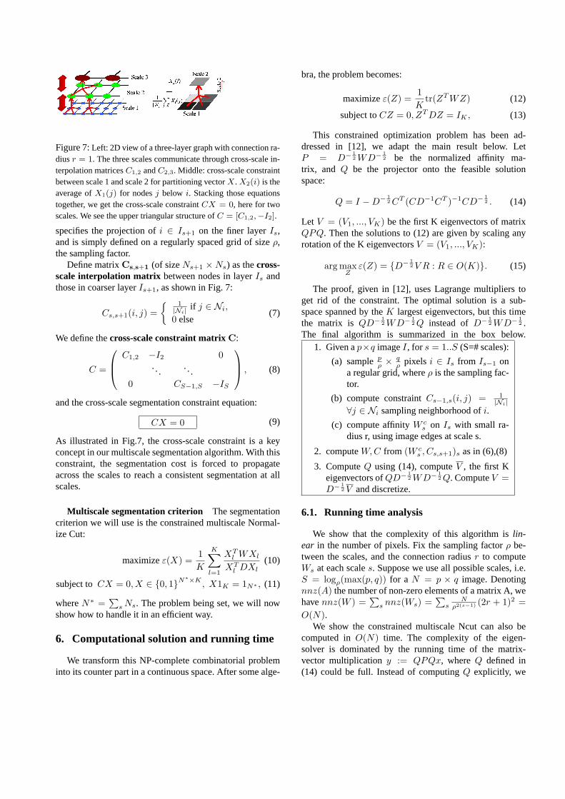
Figure 7:Left: 2D view of a three-layer graph with connection ra-diusr = 1. The three scales communicate through cross-scale in-terpolation matricesC1,2 andC2,3. Middle: cross-scale constraintbetween scale 1 and scale 2 for partitioning vectorX. X2(i) is theaverage ofX1(j) for nodesj below i. Stacking those equationstogether, we get the cross-scale constraintCX = 0, here for twoscales. We see the upper triangular structure ofC = [C1,2,−I2].

specifies the projection ofi ∈ Is+1 on the finer layerIs,and is simply defined on a regularly spaced grid of sizeρ,the sampling factor.

Define matrixCs,s+1 (of sizeNs+1 ×Ns) as thecross-scale interpolation matrix between nodes in layerIs andthose in coarser layerIs+1, as shown in Fig. 7:

Cs,s+1(i, j) ={ 1

|Ni| if j ∈ Ni,

0 else(7)

We define thecross-scale constraint matrixC:

C =

C1,2 −I2 0. ..

.. .0 CS−1,S −IS

, (8)

and the cross-scale segmentation constraint equation:

CX = 0 (9)

As illustrated in Fig.7, the cross-scale constraint is a keyconcept in our multiscale segmentation algorithm. With thisconstraint, the segmentation cost is forced to propagateacross the scales to reach a consistent segmentation at allscales.

Multiscale segmentation criterion The segmentationcriterion we will use is the constrained multiscale Normal-ize Cut:

maximizeε(X) =1K

K∑

l=1

XTl WXl

XTl DXl

(10)

subject toCX = 0, X ∈ {0, 1}N∗×K, X1K = 1N∗ , (11)

whereN∗ =∑

s Ns. The problem being set, we will nowshow how to handle it in an efficient way.

6. Computational solution and running time

We transform this NP-complete combinatorial probleminto its counter part in a continuous space. After some alge-

bra, the problem becomes:

maximizeε(Z) =1K

tr(ZT WZ) (12)

subject toCZ = 0, ZT DZ = IK , (13)

This constrained optimization problem has been ad-dressed in [12], we adapt the main result below. LetP = D− 1

2 WD− 12 be the normalized affinity ma-

trix, and Q be the projector onto the feasible solutionspace:

Q = I −D− 12 CT (CD−1CT )−1CD− 1

2 . (14)

Let V = (V1, ..., VK) be the first K eigenvectors of matrixQPQ. Then the solutions to (12) are given by scaling anyrotation of the K eigenvectorsV = (V1, ..., VK):

arg maxZ

ε(Z) = {D− 12 V R : R ∈ O(K)}. (15)

The proof, given in [12], uses Lagrange multipliers toget rid of the constraint. The optimal solution is a sub-space spanned by theK largest eigenvectors, but this timethe matrix is QD− 1

2 WD− 12 Q instead ofD− 1

2 WD− 12 .

The final algorithm is summarized in the box below.1. Given ap×q imageI, for s = 1..S (S=# scales):

(a) samplepρ × q

ρ pixels i ∈ Is from Is−1 ona regular grid, whereρ is the sampling fac-tor.

(b) compute constraintCs−1,s(i, j) = 1|Ni|

∀j ∈ Ni sampling neighborhood ofi.

(c) compute affinityW cs on Is with small ra-

dius r, using image edges at scale s.

2. computeW,C from (W cs , Cs,s+1)s as in (6),(8)

3. ComputeQ using (14), computeV , the first Keigenvectors ofQD− 1

2 WD− 12 Q. ComputeV =

D− 12 V and discretize.

6.1. Running time analysis

We show that the complexity of this algorithm islin-ear in the number of pixels. Fix the sampling factorρ be-tween the scales, and the connection radiusr to computeWs at each scales. Suppose we use all possible scales, i.e.S = logρ(max(p, q)) for a N = p × q image. Denotingnnz(A) the number of non-zero elements of a matrix A, wehavennz(W ) =

∑s nnz(Ws) =

∑s

Nρ2(s−1) (2r + 1)2 =

O(N).We show the constrained multiscale Ncut can also be

computed inO(N) time. The complexity of the eigen-solver is dominated by the running time of the matrix-vector multiplicationy := QPQx, whereQ defined in(14) could be full. Instead of computingQ explicitly, we

expand out the terms inQ, and apply a chain of smallermatrix-vector operations. The only time consuming term iscomputation ofy := (CD−1CT )−1x, which hasO(N3)running time. However, because we chose non-overlappinggrid neighborhoods, we can order the graph nodes to makeC (and henceCD− 1

2 ) upper triangular. We then computey := (CD−1CT )−1x by solving 2 triangular systems withnnz(C) = O(N) elements. Overall, the complexity ofy := QPQx is O(N). We verified empirically this linearrunning time bound, and the results in Fig. 8 show a dra-matic improvement over state of the art implementations.

0 512^2 768^2 1024^20

500

1000

1500

2562

1282

Original Ncut

Multiscale Ncut

(a) (b)40^2 90^2 140^2 185^20

40

80

Original Ncut

Multiscale Ncut

Figure 8:Running time in seconds of original Ncut vs. Multi-scale Ncut as a function of image pixelsN . In original Ncut, wescale connection radius with image size:Gr =

√N

20, and running

time is≥ O(NG2r) = O(N2). In Multiscale Ncut, we construct

a multiscale graph with same effective connection radius. Its run-ning time isO(N).

6.2. Comparison with other multi-level graph cuts

It is important to contrast this method to two other suc-cessful multilevel graph partitioning algorithms: METIS [5]and Nystrom approximation [3]. In both cases, one adap-tively coarsens the graph into a small set of nodes, and com-pute segmentation on the coarsened graph. The fine levelsegmentation is obtained byinterpolation. Both algorithmsrequire correct initial graph coarsening [3]. Nystrom worksquite well for grouping cues such as color. However for in-tervening contour grouping cues, graph weights have abruptvariations making such precise graph coarsening infeasible.

7. Results

Sanity check.We verify Multiscale Ncut segmentation witha simple “tree” image shown in Fig. 9. We create two scales,with sampling rate = 3. The first level graph has radius =1,the second level has radius = 9. We test whether Multi-scale Ncut is able to segment coarse and fine structures atthe same time: the large trunk as well as the thin branches.

For comparison, we computed Ncut eigenvectors of coarseand fine level graphs in isolation. As we see in Fig.9, mul-tiscale segmentation performs correctly, combining benefitsof both scales.

Figure 9:Top middle: fine level segmentation fails in cluttered re-gion; Bottom left, coarse level segmentation alone fails to providedetailed boundary; Bottom middle multiscale segmentation pro-vides correct global segmentation with detailed boundary. Right:zoom portion of the segmentation in fine level (a), coarse level (b),and multiscale (c).

Effect of sampling error in coarse graph construction.Wepurposely kept construction of multiscale graph extremelysimple with geometric sampling. This sampling could havea bad effect on pixels near an object boundary. We study ifMultiscale Ncut can overcome this sampling error. Fig. 10shows the final segmentation can overcome errors in coarsegrid quantization, with a small decrease in boundary sharp-ness (defined as eigenvector gap across the object bound-ary) in worst case.

Effect of image clutter and faint contoursWe argue multi-scale segmentation can handle image clutter and detect ob-jects with faint contours. Such a problem is particularly im-portant for segmenting large images. Fig. 11 provides onesuch example with a800× 700 image. The segmentation isboth accurate (in finding details), robust (in detecting faintbut elongated object boundary), and fast.

We have experimented with the multiscale Ncut on avariety of natural images, shown in Fig. 12. We observedthat compressed long range graph connections significantlyimprove running time and quality of segmentation. Morequantitative measurement is currently underway.

References

[1] Adrian Barbu and Song-Chun Zhu. Graph partition byswendsen-wang cuts. InInt. Conf. Computer Vision, pages320–327, Nice, France, 2003.

Figure 10:Non-adaptive grid can produce precise object bound-aries and recover from errors in grid quantization. Top: a two levelgraph, with coarse nodes spaced on a regular grid (boundaries inred). An object boundary (in blue) specifies two regions (green vs.blue) with low mutual affinity. Its locationd (as% of grid size)w.r.t. the grid varies fromd = 0% (best case, grid and objectboundaries agree) tod = 50% (worst case, object boundary cutsthe grid in half). The central coarse node is linked either to left orright coarse nodes depending ond. Bottom: multiscale Ncut eigen-vector ford = 0%, 25%, 50%. In all cases, multiscale segmenta-tion recovers from errors in coarse level grid. Notice that the gapin Ncut eigenvector across the object boundary remains high evenin worst case.

[2] Peter J. Burt and Edward H. Adelson. The laplacian pyramidas a compact image code. COM-31(4):532–540, April 1983.

[3] C. Fowlkes, S. Belongie, F. Chung, and J. Malik. Spectralgrouping using the nystrom method. 2003.

[4] J-M. Jolion and A. Rosenfeld.A Pyramid Framework forEarly Vision. Kluwer Academic Publishers, Norwell, MA,1994.

[5] George Karypis and Vipin Kumar. Multilevel k-way parti-tioning scheme for irregular graphs. 1995.

[6] T. Lindeberg. Edge detection and ridge detection with auto-matic scale selection. pages 465–470, 1996.

[7] M. Luettgen, W. Karl, A. Willsky, and R. Tenney. Multiscalerepresentations of markov random fields. pages 41:3377–3396, 1993.

[8] Patrick Perez and Fabrice Heitz. Restriction of a markovrandom field on a graph and multiresolution image analysis.Technical Report RR-2170.

[9] Eitan Sharon, Achi Brandt, and Ronen Basri. Fast multiscaleimage segmentation. InIEEE Conference on Computer Vi-sion and Pattern Recognition, pages 70–7, 2000.

[10] Jianbo Shi and Jitendra Malik. Normalized cuts and imagesegmentation.IEEE Transactions on Pattern Analysis andMachine Intelligence, 22(8):888–905, 2000.

[11] Stella X. Yu. Segmentation using multiscale cues. InIEEEConference on Computer Vision and Pattern Recognition,pages 70–7, 2004.

[12] Stella X. Yu and Jianbo Shi. Grouping with bias. InAd-vances in Neural Information Processing Systems, 2001.

1

2

3

4

5

6

7

8

9

10

11

12

13

Edge

EdgeEdge

Ncut Eigenvector Ncut Eigenvector

Ncut Eigenvector

Ncut Eigenvector

Segmentation

Figure 11:Multiscale Ncut segmentation of a800 × 700 image.Top left, image with detected object boundary. Top right, segmen-tation and input edge map. Bottom: zoom in details. Note the faintroof boundary is segmented clearly.

Figure 12:Multiscale Ncut prevents braking large uniform im-age regions into smaller parts due to its efficient use of long rangegraph connections.