Stock Return Volatility and World WarII: Evidence From Garch and Garch-XModels

Taufiq ChoudhryDepartment of Economics, University of Wales, Swansea SA2 8PP, U.K.

This paper investigates volatility in the stock markets of Canada, Denmark, Sweden,Switzerland, the United Kingdom and the United States, and the effects of short-rundeviations between stock indices of these markets on the volatility during January1926–December 1944. The empirical work is conducted by means of the GARCH(1,1)and GARCH(1,1)-X models. Both tests provide evidence of volatility clustering but lowlevel of persistence to shocks to volatility. Results from GARCH-X also indicate asignificant effect of the short-run deviations on volatility. The GARCH(1,1)-X modelseems to perform better than the standard GARCH(1,1).

KEYWORDS: volatility; GARCH; leverage effect; structural shift

SUMMARY

This paper investigates the long-run relationshipbetween stock indices of different countries and theeffect of short-run deviations from the relationshipon stock returns volatility. Monthly stock indicesfrom Canada, Denmark, Sweden, Switzerland, theUnited Kingdom and the United States duringJanuary 1926–December 1944 are applied in theempirical study. The period under study includesthe stock market crash of October 1929 and WorldWar II, among other political and economic events.The long-run relationship is investigated by meansof the cointegration tests, and the effect of short-rundeviations on stock returns volatility is studied bymeans of the GARCH models. The GARCH modelapplied takes into consideration the possiblestructural shift of volatility due to the depressionyears 1929–1933, which also include the stockmarket crash of 1929. The GARCH model alsocompensates for the possible negative correlationbetween current returns and future volatility,known as the leverage effect. Results indicate asignificant long-run relationship between the stated

indices, and results also show significant effect ofdeviations on the stock returns volatility. Thepresence of short-run deviations in the volatilityfunction may be exploited to obtain more precisepoint forecasts of stock price changes. Someevidence of the structural shift in volatility due tothe depression years is found, while very littlesupport is found for the leverage effect.

INTRODUCTION

In recent years, research on financial integrationhas been extensive (Hamao et al., 1990). It hasincluded the study of the correlation of asset pricesacross international markets (Barclay et al., 1990;Eun and Shim, 1989), common stochastic trend(s)among international assets (Choudhry, 1994; Cor-hay et al., 1993) and international volatility spil-lover (Hamao et al., 1990 and Ng et al., 1991). Thispaper extends this previous research by studyingthe effects of short-run deviations between stockindices of different countries on the stock marketvolatility. A significant positive effect would imply

CCC 1076–9307/97/010017–12 Received 30 June 1995# 1997 by John Wiley & Sons, Ltd. Int. J. Finance Economics, Vol. 2, 17–28

that prediction of stock returns may become harderas the indices move apart from each other in theshort-run.

This paper provides a study of the stock marketvolatility in six markets between 1926 and 1944 bymeans of Generalized Autoregressive ConditionalHeteroscedastic (GARCH) models. These GARCHmodels (Bollerslev, 1986) are capable of capturingthe three important most empirical features ob-served in stock return data: leptokurtosis, skew-ness, and volatility clustering.1,2 According toBollerslev et al. (1992) the GARCH model can beviewed as a reduced form of a more complicateddynamic structure for the time-varying conditionalsecond-order moments. The GARCH models pro-vide a more flexible framework to capture variousdynamic structures of conditional variance andallow simultaneous estimation of several param-eters of interest (Chou, 1988).

Recently, an extension of the standard GARCHmodel which links with the error correction models(ECM) of cointegrated series, known as theGARCH-X model, has been put forward by Lee(1994). Cointegration implies that a linear combina-tion(s) of two or more non-stationary variablesconverges to an equilibrium in the long-run,although individually these variables might driftapart in the short-run. Short-run deviations from along-run cointegrated relationship are indicated bythe error-correction term(s) from the ECM. TheGARCH-X model may be applied to investigate thepredictive power of the short-run deviationsbetween the stock indices in predicting the volati-lity of the stock returns. According to Lee (1994),examining the behaviour of the conditional var-iances over time as a function of short-rundeviations is reasonable when one expects in-creased volatility due to shocks to the systemwhich propagate on both the first and the secondmoments.

Monthly stock returns from the stock markets ofCanada, Denmark, Sweden, Switzerland, the Uni-ted Kingdom and the United States from January1926 to December 1944 are employed in theempirical work. As indicated above the time periodstudied includes most years of the second worldwar.3 According to Synder (1990) stock prices ofallied countries had a direct relationship(s) duringperiods of war. This is based on two signalsimposed on stock prices by the war, one affecting

the probability of losing and the other affecting theexpected length of the war. Both signals caused theallied nations’ stock prices to move together. Theactual empirical work is conducted by means of theJohansen’s multivariate cointegration test and theunivariate GARCH and GARCH-X models.

This paper is presented in two parts dependingon the model used; it first investigates the returnsfrom each of the markets using the GARCH modeland then, in the second part, the empirical work isconducted using the modified GARCH model, theGARCH-X. In this manner we are able to comparethe performance of the two models and also studythe effects of the war on stock market volatility. Ina preview of the results, we are able to findsignificant interaction between the six indices. Wealso find evidence of the significant effect of theshort-run deviations on the conditional variance.Results show that the GARCH-X model performsbetter than the standard GARCH model.

The bulk of the latest research involving stockreturns has been conducted for the latest periodand economic conditions (see Bollerslev et al.,1992). This paper employs stock returns data fromthe mid-1920s to mid-1940s. The period underconsideration (1926–1944) involves large changes inboth economic and political variables throughoutthe world. As shown by Schwert (1989a, 1989b)stock market volatility was affected by severaldifferent economic and financial variables. TheEuropean and the North American economyinitially recovered slowly after the negative shockimposed by the first world war (WWI), and thenrapid recovery and expansion took place from 1925to 1929 (Aldcroft, 1980). The depression of 1929–1932 resulted in large downward movements in theindustrial production and national incomethroughout Europe and North America (Aldcroft,1980). October of 1929 saw the dramatic stockmarket crash in the United States and Europe. The1920s and 1930s also saw a move back to a dilutedversion of the gold standard known as the goldexchange standard from 1925 to 1931 (Brown,1940). After WWI there was a substantial increasein international financial cooperation betweenlending nations (Einzig, 1935). This post-warinternational financial cooperation provided fundsfor countries from foreign governments, Centralbanks or the League of Nations. This internationalfinancial cooperation also enabled the borrowing

18 T. Choudhry

countries to place their finances on a sounder basis(Einzig, 1935).

The rise to power of Hitler and the Nazi party inGermany in the early 1930s created political andeconomic tension in Europe (Jeffries, 1993). Giventhat the period 1926–1944 is not without politicaland economic turbulence, it is interesting toinvestigate the stock market volatility in differentcountries, long-run relationship(s) between differ-ent stock markets and the effects of this relation-ship(s) on stock market volatility.

THE DATA AND THE COINTEGRATIONTESTS

The data

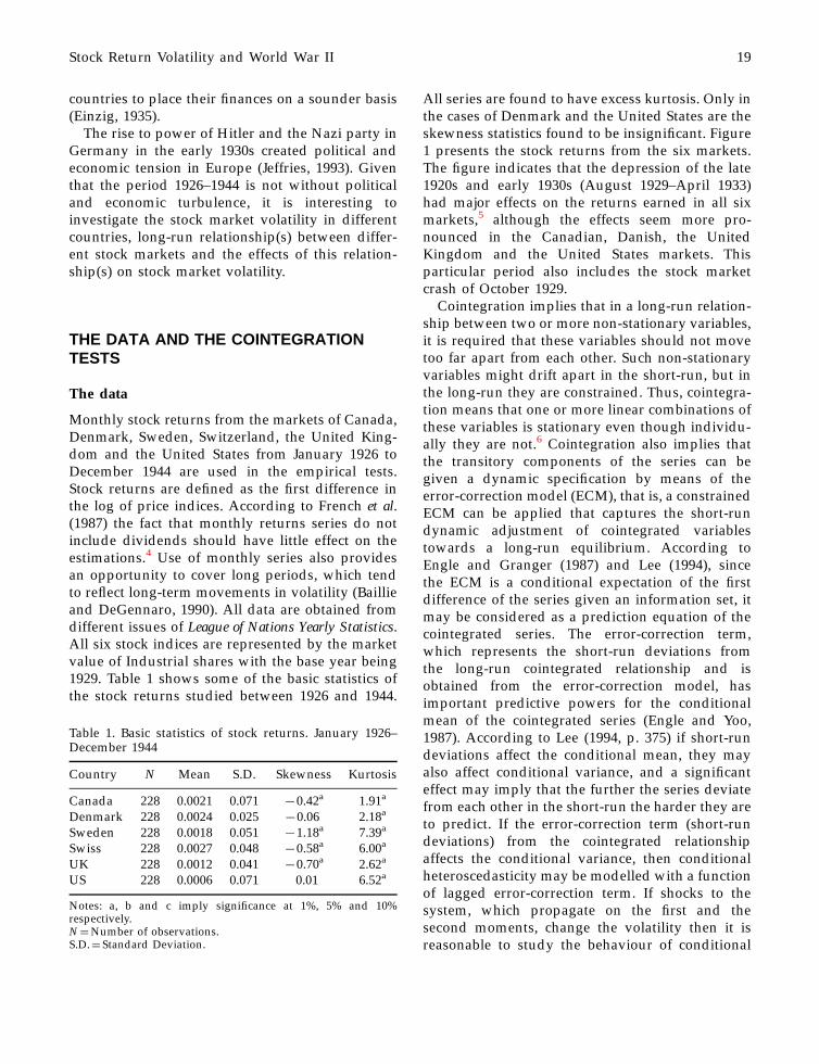
Monthly stock returns from the markets of Canada,Denmark, Sweden, Switzerland, the United King-dom and the United States from January 1926 toDecember 1944 are used in the empirical tests.Stock returns are defined as the first difference inthe log of price indices. According to French et al.(1987) the fact that monthly returns series do notinclude dividends should have little effect on theestimations.4 Use of monthly series also providesan opportunity to cover long periods, which tendto reflect long-term movements in volatility (Baillieand DeGennaro, 1990). All data are obtained fromdifferent issues of League of Nations Yearly Statistics.All six stock indices are represented by the marketvalue of Industrial shares with the base year being1929. Table 1 shows some of the basic statistics ofthe stock returns studied between 1926 and 1944.

All series are found to have excess kurtosis. Only inthe cases of Denmark and the United States are theskewness statistics found to be insignificant. Figure1 presents the stock returns from the six markets.The figure indicates that the depression of the late1920s and early 1930s (August 1929–April 1933)had major effects on the returns earned in all sixmarkets,5 although the effects seem more pro-nounced in the Canadian, Danish, the UnitedKingdom and the United States markets. Thisparticular period also includes the stock marketcrash of October 1929.

Cointegration implies that in a long-run relation-ship between two or more non-stationary variables,it is required that these variables should not movetoo far apart from each other. Such non-stationaryvariables might drift apart in the short-run, but inthe long-run they are constrained. Thus, cointegra-tion means that one or more linear combinations ofthese variables is stationary even though individu-ally they are not.6 Cointegration also implies thatthe transitory components of the series can begiven a dynamic specification by means of theerror-correction model (ECM), that is, a constrainedECM can be applied that captures the short-rundynamic adjustment of cointegrated variablestowards a long-run equilibrium. According toEngle and Granger (1987) and Lee (1994), sincethe ECM is a conditional expectation of the firstdifference of the series given an information set, itmay be considered as a prediction equation of thecointegrated series. The error-correction term,which represents the short-run deviations fromthe long-run cointegrated relationship and isobtained from the error-correction model, hasimportant predictive powers for the conditionalmean of the cointegrated series (Engle and Yoo,1987). According to Lee (1994, p. 375) if short-rundeviations affect the conditional mean, they mayalso affect conditional variance, and a significanteffect may imply that the further the series deviatefrom each other in the short-run the harder they areto predict. If the error-correction term (short-rundeviations) from the cointegrated relationshipaffects the conditional variance, then conditionalheteroscedasticity may be modelled with a functionof lagged error-correction term. If shocks to thesystem, which propagate on the first and thesecond moments, change the volatility then it isreasonable to study the behaviour of conditional

Table 1. Basic statistics of stock returns. January 1926–December 1944

Country N Mean S.D. Skewness Kurtosis

Canada 228 0.0021 0.071 70.42a 1.91a

Denmark 228 0.0024 0.025 70.06 2.18a

Sweden 228 0.0018 0.051 71.18a 7.39a

Swiss 228 0.0027 0.048 70.58a 6.00a

UK 228 0.0012 0.041 70.70a 2.62a

US 228 0.0006 0.071 0.01 6.52a

Notes: a, b and c imply significance at 1%, 5% and 10%respectively.N�Number of observations.S.D.� Standard Deviation.

Stock Return Volatility and World War II 19

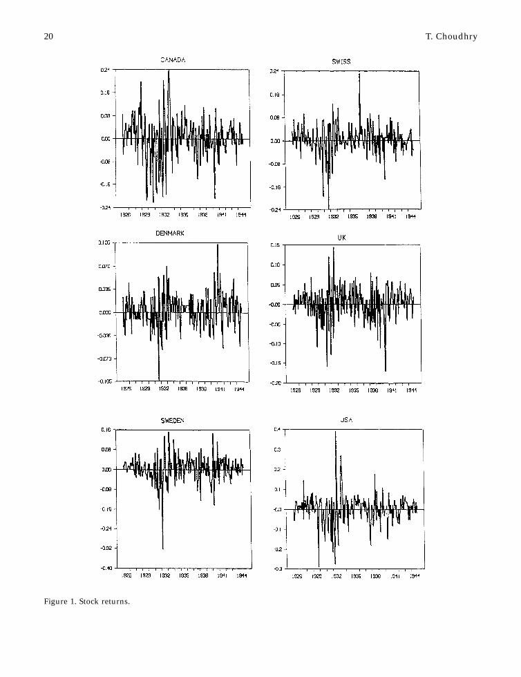
Figure 1. Stock returns.

20 T. Choudhry

variance as a function of short-run deviations (Lee,1994).

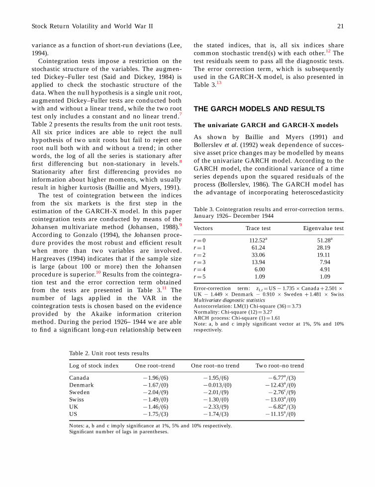
Cointegration tests impose a restriction on thestochastic structure of the variables. The augmen-ted Dickey–Fuller test (Said and Dickey, 1984) isapplied to check the stochastic structure of thedata. When the null hypothesis is a single unit root,augmented Dickey–Fuller tests are conducted bothwith and without a linear trend, while the two roottest only includes a constant and no linear trend.7

Table 2 presents the results from the unit root tests.All six price indices are able to reject the nullhypothesis of two unit roots but fail to reject oneroot null both with and without a trend; in otherwords, the log of all the series is stationary afterfirst differencing but non-stationary in levels.8

Stationarity after first differencing provides noinformation about higher moments, which usuallyresult in higher kurtosis (Baillie and Myers, 1991).

The test of cointegration between the indicesfrom the six markets is the first step in theestimation of the GARCH-X model. In this papercointegration tests are conducted by means of theJohansen multivariate method (Johansen, 1988).9

According to Gonzalo (1994), the Johansen proce-dure provides the most robust and efficient resultwhen more than two variables are involved.Hargreaves (1994) indicates that if the sample sizeis large (about 100 or more) then the Johansenprocedure is superior.10 Results from the cointegra-tion test and the error correction term obtainedfrom the tests are presented in Table 3.11 Thenumber of lags applied in the VAR in thecointegration tests is chosen based on the evidenceprovided by the Akaike information criterionmethod. During the period 1926– 1944 we are ableto find a significant long-run relationship between

the stated indices, that is, all six indices sharecommon stochastic trend(s) with each other.12 Thetest residuals seem to pass all the diagnostic tests.The error correction term, which is subsequentlyused in the GARCH-X model, is also presented inTable 3.13

THE GARCH MODELS AND RESULTS

The univariate GARCH and GARCH-X models

As shown by Baillie and Myers (1991) andBollerslev et al. (1992) weak dependence of succes-sive asset price changes may be modelled by meansof the univariate GARCH model. According to theGARCH model, the conditional variance of a timeseries depends upon the squared residuals of theprocess (Bollerslev, 1986). The GARCH model hasthe advantage of incorporating heteroscedasticity

Table 2. Unit root tests results

Log of stock index One root–trend One root–no trend Two root–no trend

Canada 71.96=(6) 71.95=(6) 76.77a=(3)

Denmark 71.67=(0) 70.013=(0) 712.43a=(0)

Sweden 72.04=(9) 72.01=(9) 72.76c=(9)

Swiss 71.49=(0) 71.30=(0) 713.03a=(0)

UK 71.46=(6) 72.33=(9) 76.82a=(3)

US 71.75=(3) 71.74=(3) 711.15a=(0)

Notes: a, b and c imply significance at 1%, 5% and 10% respectively.Significant number of lags in parentheses.

Table 3. Cointegration results and error-correction terms.January 1926– December 1944

Vectors Trace test Eigenvalue test

r� 0 112.52a 51.28a

r� 1 61.24 28.19r� 2 33.06 19.11r� 3 13.94 7.94r� 4 6.00 4.91r� 5 1.09 1.09

Error-correction term: z1;t �US7 1.7356Canada� 2.5016UK 7 1.449 6 Denmark 7 0.910 6 Sweden � 1.481 6 SwissMultivariate diagnostic statisticsAutocorrelation: LM(1) Chi-square (36)� 3.73Normality: Chi-square (12)� 3.27ARCH process: Chi-square (1)� 1.61Note: a, b and c imply significant vector at 1%, 5% and 10%respectively.

Stock Return Volatility and World War II 21

into the estimation procedure; the model capturesthe tendency for volatility clustering in financialand economic data. Individual stock returns canbe represented by the following univariateGARCH(p, q) model:

yt � mt � et �1�

et=Otÿ1 � N �0; ht� �2�

ht � a0 �Pp

j�1bjhtÿj �

Pq

j�1aj�etÿj�

2; �3�

where yt is the stock return, mt is the mean yt

conditional on past information (Otÿ1) and thefollowing inequality restrictions a0 > 0, aj� 0, andbj� 0 are imposed to ensure that the conditionalvariance (ht) is positive. The significance of aj

implies the existence of the ARCH process in theerror term. The ARCH process indicates volatilityclustering in the data. The size and significance ofaj indicates the magnitude of the effect imposed bythe lagged error term (etÿj) on the conditionalvariance (ht). Economic interpretation of the ARCHeffect in stock markets has been provided withinboth the micro and macro framework. According toBollerslev et al. (1992, p. 32) and other studies, theARCH effect in stock returns could be due toclustering of trade volumes, nominal interest rates,dividend yields, money supply, oil price changes,etc.14 According to Bera and Higgins (1993) if theseries being forecast displays ARCH, the currentinformation set can indicate the accuracy withwhich this can be done.

Along with the leptokurtic distribution of stockreturn data, negative correlation between currentreturns and future volatility have been shown byempirical research (Black, 1976; Christie, 1982).This negative effect of current returns on futurevariance is sometimes called the leverage effect(Bollerslev et al., 1992). The leverage effect is due tothe reduction in the equity value which would raisethe debt-to-equity ratio, hence raising the riskinessof the firm as a result of an increase in futurevolatility. Consequently, the future volatility will benegatively related to the current return on the stock(Black, 1976; Christie, 1982). Glosten et al. (1993)provided an alternative explanation for the nega-tive effect; if most of the fluctuations in stock pricesare caused by fluctuations in expected future cashflows and the riskiness of future cash flows doesnot change proportionally when investors revise

their expectations, then unanticipated changes instock prices and returns will be negatively relatedto unanticipated changes in future volatility. Thesymmetric (linear) GARCH model presented inEquations (1), (2) and (3) is not able to capture thisdynamic pattern because the conditional varianceis only linked to past conditional variances andsquared innovations, and hence the sign of returnsplays no role in affecting volatilities (Bollerslev etal., 1992). Glosten et al. (1993) provided a modifica-tion in the GARCH model that allows positive andnegative innovations to returns to have differentimpact on conditional variance. This modificationinvolves adding a dummy variable (It) on theinnovations in the conditional variance equation,i.e. Equation (3).15

According to Poterba and Summers (1986) theimpact of volatility on the stock prices can only besignificant if shocks to volatility persist over a longtime. The market will not make an adjustment ofthe future discount rate if shocks to volatility arenot permanent; expected stock returns are notaffected by the volatility movement if shocks tovolatility are transitory. According to Engle andBollerslev (1986), in a GARCH(1,1) model ifa� b� 1, this implies two things: persistence of aforecast of the conditional variance over all finitehorizons, and an infinite variance for the uncondi-tional distribution of et. In other words, whena� b� 1 current shock persists indefinitely inconditioning the future variance. In a GARCH(1,1)model the et is covariance stationary if the sum of aand b is significantly less than unity. As the sum ofa and b approaches unity the persistence of shocksto volatility is greater. Since a� b represents thechange in the response function of shocks tovolatility per period, a value greater than unityimplies that the response function of volatilityincreases with time, and a value less than unityimplies that shocks decay over time (Chou, 1988).The closer the value of persistence measurement isto unity, the slower is the decay rate.16

According to Lamoureux and Lastrapes (1990)the GARCH model may provide biased upwardestimates of persistence in variance if deterministicor structural shifts in the unconditional varianceare unaccounted for. Diebold (1986) and Lamour-eux and Lastrapes (1990) have demonstrated thatthe presence of structural shifts may make theconstant term (a0) in the conditional variance

22 T. Choudhry

equation unstable over the sample period. Lamour-eux and Lastrapes (1990) further claim that thelonger the sample period, the higher the prob-ability that structural shifts will be present. Asadvocated by these studies, possible structuralshifts in conditional variance may be accountedfor by including dummy variables representingperiod(s) of such possible shifts in the conditionalvariance equation of a GARCH(1,1) model:

ht � a0 � d0Dt � b1htÿ1 � a1�etÿ1�2 � a2�etÿ1�

2Itÿ1

�3a�

where Dt is the dummy variable that takes thevalue of one during period(s) of possible shift(s)and zero otherwise, and Itÿ1 is the leverage effectdummy variable that takes the value one when etÿ1

is positive, and zero when etÿ1 is negative. Every-thing else is defined as earlier. As indicated inFigure 1, the recession period of 1929–1933 whichalso includes the market crash of October 1929seems to have an adverse effect(s) on stock returnsin all six markets.17 Thus, the depression years(1929–1933) are considered to be a period whichmay have resulted in the structural shifts of theunconditional variance.18 In Equation (3a) thestructural shift dummy variable (Dt) takes on thevalue of one between August 1929 and April 1933,and zero during other periods. The dummyvariable (Itÿ1) is added to capture the leverageeffect as advocated by Glosten et al. (1993). TheGARCH(1,1) model applied here consists of Equa-tions (1), (2) and (3a). In this particular form of theGARCH(1,1) model the persistence of shock mea-surement is equal to a1� a2� b1.

As stated above, the GARCH-X model takes intoconsideration the effects of the short-run deviationson the conditional variance:

ht � a0 � d0Dt � b1htÿ1 � a1�etÿ1�2

� a2�etÿ1�2Itÿ1 � g1�ztÿ1�

2: �3b�

The short-run deviations represented by the laggederror-correction term(s) (ztÿ1) are included in themodel, squared and lagged once as advocated byLee (1994, p. 377). The parameter g1 indicates theeffects of the short-run deviations between the sixstock indices from a long-run cointegrated relation-ship on the conditional variance of the residuals ofthe returns equation. Using this model, the pre-dictive power of the spread between monthly stock

indices from the six markets in predicting volatilityof the stock market returns may be investigated. Ifthe squared error-correction terms are positivelyrelated to the conditional variance, this implies thatthe stock prices become more volatile and harder topredict as the spread between the two prices getslarger (Lee 1994, p. 376). Thus, the presence of theshort-run deviations in the conditional variancefunction may be exploited to obtain more precisetime-varying confidence intervals for point fore-casts of stock price changes. Definitions of othervariables stay the same. The GARCH(1,1)-X modelapplied in this paper consists of Equations (1), (2)and (3b).

GARCH and GARCH-X Results

Tables 4 and 5 show results from the univariateGARCH(1,1) and GARCH(1,1)-X modelsrespectively.19 Table 4 shows the ARCH processto be present in four out of the six series.20 The twoseries without the ARCH process are from Canadaand Switzerland. The four significant ARCHcoefficients are much smaller than unity and thusshocks to conditional variance are not explosive.The dummy variable (Dt) representing the depres-sion period is found to be positive in all six testsand significant only in the cases of Canada,Denmark and the United States. The significanceof the depression years dummy variables indicatesthe presence of structural shifts in unconditionalvariance due to the depression of the 1920s and1930s. The leverage effect dummy variable (Itÿ1) isnegative and only significant in the case of theUnited Kingdom.21 A significant and negativeleverage effect dummy coefficient implies that,along with the size, the sign of the error term hasan important effect on volatility. Thus, in the case ofthe United Kingdom, conditional variance is higherwhenever innovations (etÿ1) to returns are negativerather than positive. All residuals are leptokurticand, except for Denmark and the United States, allresiduals are also significantly skewed to the left.No significant serial correlation at the 5% level isshown by the Box–Ljung statistics. The persistencemeasurement (a1� a2� b1) indicates that only inthe Swedish market may shocks to volatility bepermanent. In the remaining cases the persistencemeasurement is well below unity, implying transi-tory shocks to volatility.22,23

Stock Return Volatility and World War II 23

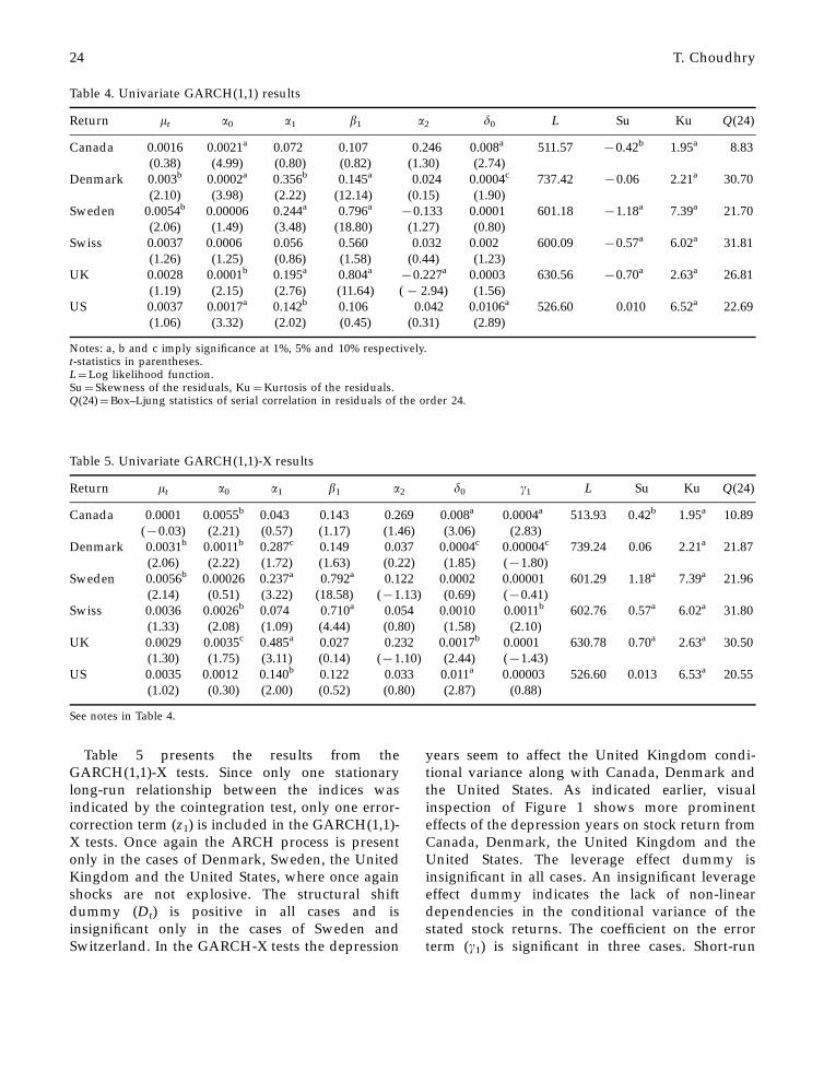
Table 5 presents the results from theGARCH(1,1)-X tests. Since only one stationarylong-run relationship between the indices wasindicated by the cointegration test, only one error-correction term (z1) is included in the GARCH(1,1)-X tests. Once again the ARCH process is presentonly in the cases of Denmark, Sweden, the UnitedKingdom and the United States, where once againshocks are not explosive. The structural shiftdummy (Dt) is positive in all cases and isinsignificant only in the cases of Sweden andSwitzerland. In the GARCH-X tests the depression

years seem to affect the United Kingdom condi-tional variance along with Canada, Denmark andthe United States. As indicated earlier, visualinspection of Figure 1 shows more prominenteffects of the depression years on stock return fromCanada, Denmark, the United Kingdom and theUnited States. The leverage effect dummy isinsignificant in all cases. An insignificant leverageeffect dummy indicates the lack of non-lineardependencies in the conditional variance of thestated stock returns. The coefficient on the errorterm (g1) is significant in three cases. Short-run

Table 5. Univariate GARCH(1,1)-X results

Return mt a0 a1 b1 a2 d0 g1 L Su Ku Q(24)

Canada 0.0001 0.0055b 0.043 0.143 0.269 0.008a 0.0004a 513.93 0.42b 1.95a 10.89(70.03) (2.21) (0.57) (1.17) (1.46) (3.06) (2.83)

Denmark 0.0031b 0.0011b 0.287c 0.149 0.037 0.0004c 0.00004c 739.24 0.06 2.21a 21.87(2.06) (2.22) (1.72) (1.63) (0.22) (1.85) (71.80)

Sweden 0.0056b 0.00026 0.237a 0.792a 0.122 0.0002 0.00001 601.29 1.18a 7.39a 21.96(2.14) (0.51) (3.22) (18.58) (71.13) (0.69) (70.41)

Swiss 0.0036 0.0026b 0.074 0.710a 0.054 0.0010 0.0011b 602.76 0.57a 6.02a 31.80(1.33) (2.08) (1.09) (4.44) (0.80) (1.58) (2.10)

UK 0.0029 0.0035c 0.485a 0.027 0.232 0.0017b 0.0001 630.78 0.70a 2.63a 30.50(1.30) (1.75) (3.11) (0.14) (71.10) (2.44) (71.43)

US 0.0035 0.0012 0.140b 0.122 0.033 0.011a 0.00003 526.60 0.013 6.53a 20.55(1.02) (0.30) (2.00) (0.52) (0.80) (2.87) (0.88)

See notes in Table 4.

Table 4. Univariate GARCH(1,1) results

Return mt a0 a1 b1 a2 d0 L Su Ku Q(24)

Canada 0.0016 0.0021a 0.072 0.107 0.246 0.008a 511.57 70.42b 1.95a 8.83(0.38) (4.99) (0.80) (0.82) (1.30) (2.74)

Denmark 0.003b 0.0002a 0.356b 0.145a 0.024 0.0004c 737.42 70.06 2.21a 30.70(2.10) (3.98) (2.22) (12.14) (0.15) (1.90)

Sweden 0.0054b 0.00006 0.244a 0.796a70.133 0.0001 601.18 71.18a 7.39a 21.70

(2.06) (1.49) (3.48) (18.80) (1.27) (0.80)Swiss 0.0037 0.0006 0.056 0.560 0.032 0.002 600.09 70.57a 6.02a 31.81

(1.26) (1.25) (0.86) (1.58) (0.44) (1.23)UK 0.0028 0.0001b 0.195a 0.804a

70.227a 0.0003 630.56 70.70a 2.63a 26.81(1.19) (2.15) (2.76) (11.64) (7 2.94) (1.56)

US 0.0037 0.0017a 0.142b 0.106 0.042 0.0106a 526.60 0.010 6.52a 22.69(1.06) (3.32) (2.02) (0.45) (0.31) (2.89)

Notes: a, b and c imply significance at 1%, 5% and 10% respectively.t-statistics in parentheses.L�Log likelihood function.Su� Skewness of the residuals, Ku�Kurtosis of the residuals.Q(24)�Box–Ljung statistics of serial correlation in residuals of the order 24.

24 T. Choudhry

deviations do not seem to impose any effect on thestock market volatility in Sweden, the UnitedKingdom and the United States between 1926–1944.24 In the Danish and Swiss tests, the errorcorrection term coefficient (g1) is significant andnegative, although in absolute value the sizes of thecoefficients are very small. Significant negativecoefficients imply an inverse relationship betweenvolatility and short-run deviations, which in turnindicate that prediction of return becomes moredifficult as the deviations between the indicesdecrease in the short-run. The Canadian testprovides a positive and significant effect of theerror correction term on the conditional variance.Thus, as the short- run deviations between theindices increase, Canadian stock returns volatilityalso increases. Once again all residuals from thetests are leptokurtic and, except for the Danish andthe United States case, the residuals are alsosignificantly skewed to the left. The Box–Ljungstatistics fail to indicate serial correlation at the 5%level in any of the residuals. Only in the case ofSweden do we find some evidence of permanentshocks to volatility.25

Comparing the two models, based on the log-likelihood function value, the GARCH(1,1)-Xseems to perform better than the GARCH(1,1),though the differences are negligible. Using theGARCH(1,1)-X, we are able to find some moreevidence of the structural shift due to the depres-sion years but less evidence of a leverage effect.The size and significance of the ARCH coefficient issimilar in both models. There is some difference inthe measurement of persistence of shocks tovolatility. For Switzerland the persistence measure-ment increases by a considerable amount in theGARCH(1,1)-X model while for the United King-dom the measurement decreases substantially.Measurements in other markets do not varyaccording to the two tests. Both models alsoprovide very similar results involving the diag-nostic structure of the test residuals.

CONCLUSIONS

This paper investigates the stock returns volatilityand the effects of the short-run deviations betweenstock indices on stock returns volatility in the

markets of Canada, Denmark, Sweden, Switzer-land, the United Kingdom and the United Statesduring January 1926–December 1944. The empiri-cal work is conducted using monthly stock returnsand univariate Generalized ARCH (GARCH) andGARCH-X models. Short-run deviations betweenthe six indices are indicated by the error correctionterm from the cointegration tests between thestated indices. Cointegration tests indicate station-ary long-run relationship(s) between the six stockindices during the stated period. Both theGARCH(1,1) and GARCH(1,1)-X also includedummy variables to account for the possiblestructural shifts of the unconditional varianceduring the depression years (1929–1933) andthe leverage effect, which implies that positiveand negative innovations have different effectson conditional variance. Results from theGARCH(1,1)-X model indicate a significant effectimposed by the deviations on the volatility in someof the stock markets under study. These resultsimply that more precise forecasts of changes instock prices may be obtained. Results from bothmodels also the imply ARCH effect but theseeffects are not very explosive. Very little evidenceof permanent shocks to volatility is found by eithertest. Some evidence of the structural shift in theunconditional variance due to the depression yearsis also found, while very little support is found forthe leverage effect. Results in this paper alsoadvocate the need for similar research using highfrequency stock return data, such as daily dataduring the latest period.

ENDNOTES

1. Bollerslev (1987), Bollerslev et al. (1988), French et al.(1987), Baillie and DeGennaro (1990) apply theGARCH models in explaining the distribution ofcommon stock prices. See Bollerslev et al. (1992) foran excellent survey on the application of the GARCHmodels in financial and economic studies.

2. Starting with the pioneering work of Mandelbrot(1963) and Fama (1965), empirical research has foundevidence that large changes in stock prices arefollowed by large changes of either sign, and thatsmall changes are followed by small changes ofeither sign; this research also indicates that changesin stock prices exhibit fatter tails than a normaldistribution. In other words, earlier research con-

Stock Return Volatility and World War II 25

firms unconditional distribution of security pricechange to be leptokurtic, skewed, and volatilityclustered.

3. The second world war in Europe started with theinvasion of Poland by Germany in September of1939. The war ended in 1945 (both in Europe andAsia), but lack of data for some countries limited thedates used here to 1944.

4. This is true because the ex-dividend days aredifferent for different stocks in an index and thechanges in the stock index due to dividend paymentsare not large. Furthermore, according to Shiller (1981)variation due to dividends is too small to beconsistent with the huge variance of the stock prices.

5. The dates for depression years were taken fromFriedman and Schwartz (1971).

6. Detailed analyses of cointegration are available innumerous articles and books, for example Engle andGranger (1987) and Dickey and Rossana (1994).

7. The number of lags applied in the augmentedDickey–Fuller test is chosen based on the evidenceprovided by the Akaike Information Criterion. Themaximum number of lags applied in the unit roottests is 12.

8. A single unit root in stock indices may provideevidence of a weak form of efficient market(Choudhry, 1994).

9. Detail analyses of the Johansen method are providedin several articles and books, such as Dickey andRossana (1994) and Harris (1995). In order topreserve space an analysis is not provided in thispaper.

10. Hargreaves, applying Monte Carlo simulations,found the lowest mean bias and median bias in theJohansen method compared with other cointegrationmethods when the number of data is 100 or more.

11. All cointegration tests were conducted with the CATSprogram in computer package RATS version 4.20.

12. The presence of a significant common stochasticvector(s) may indicate evidence against the semi-strong form of market efficiency (Choudhry, 1994).

13. Restriction tests by means of the likelihood ratio testindicate that the coefficients on the United Statesindex and Swedish index are not equal to each other.Similarly, coefficients on the Danish and Swissindices are also not found to be equal to each other.

14. Bera and Higgins (1993, p. 322) provide severaldifferent interpretations of the ARCH process in-cluding clustering of large and small errors, andexcess kurtosis.

15. There is more than one GARCH model available thatis able to capture the leverage effect. Pagan andSchwert (1990), Engle and Ng (1993) and Hentschel(1995) provide excellent analyses and comparison ofsymmetric and asymmetric GARCH models. Accord-ing to Engle and Ng (1993) the GJR model is the bestat parsimoniously capturing this asymmetric effect.

16. Several papers provide evidence of high persistenceof shocks to the stock return volatility in several

markets (see for example, French et al., 1987; Chou,1988; Choudhry, 1995).

17. During August 1929 to April 1933, mean returns inall six markets were negative. The following repre-sents the actual mean return in each case: Canada70.0040, Denmark 70.0012, Sweden 70.0091, Swit-zerland 70.0025, UK 70.0023 and US 70.0088. Theactual rate of change in the indices from September1929 to October 1929 are: Canada 72.53%, Denmark2.33%, Sweden 0.00%, Switzerland 72.70%, UK0.00% and US 71.83%. Daily data would probablyshow better movement of the stock indices aroundthe crash date.

18. As indicated by Lamoureux and Lastrapes (1990, p.226) the problem in performing this test is thedetermination of the actual timing of the structuralshift. Officer (1973), Schwert (1989a, 1989b) andPagan and Schwert (1990) claim that during financialand economic crises, such as recessions and depres-sions, stock market volatility is unusually high.

19. All GARCH models were estimated by means of theBerndt et al. (1974) algorithm in the RATS version4.20 computer package.

20. As stated earlier, the ARCH effect in stock returncould be due to several reasons. To investigate thereason(s) behind the ARCH effect in these markets isbeyond the theme of this paper but is an incentive forfuture research.

21. The coefficient of the leverage dummy (a2) as well asa1� a2 may be negative as empirical evidencesuggests that a positive innovation to stock returnis associated with a decrease in return volatility(Glosten et al., 1993, p. 1788).

22. According to Lamoureux and Lastrapes (1990) thehalf- life of the shocks is equal to 1 ÿ �log 2=og�a1 � b1�� and it measures the period of time(number of months) over which a shock to volatilitydiminishes to half its original size. In the case ofSweden half- life is more than eight months and forthe United States it is about one and half months. Thedecay rate of the impact is much slower in theSwedish market.

23. Persistence measurements were much higher usingof the standard GARCH(1,1) model without anydummies for the potential structural shifts andleverage effect. These results are not provided inorder to save space but are available on request.Reduction in the persistence could be due to thestructural shift in the conditional variance caused bythe depression years. The GARCH(1,1) with thedummies seems to perform better than withoutdummies.

24. The GARCH(1,1)-X model without any dummies forthe structural shifts and leverage effect providesmore evidence of the effects of the short-rundeviations; the performance of the GARCH-X modelwith the dummies is better in all cases. Results fromthe GARCH(1,1)-X without any dummies are avail-able on request.

26 T. Choudhry

25. The GARCH(1,1)-X model without any dummies forthe structural shifts and leverage effect provide moreevidence of permanent shocks to volatility. Theseresults are available on request.

REFERENCES

Aldcroft, D. (1980), The European Economy 1914–1980,London: Billing & Sons Ltd.

Baillie, R. and Myers, R. (1991), Bivariate GARCHestimation of the optimal commodity futures hedge.Journal of Applied Econometrics, 6, 109–124.

Baillie, R. and DeGennaro, R. (1990), Stock returns andvolatility. Journal of Financial and Quantitative Analysis,25, 203–214.

Barclay, M., Litzenberger, R. and Warner, J. (1990), Privateinformation, trading volume, and stock-returnvariance. Review of Financial Studies, 3, 233–253.

Bera, A. and Higgins, M. (1993), ARCH models: proper-ties, estimation and testing. Journal of Economic Surveys,7, 305–366.

Berndt, E., Hall, B., Hall, R. and Hausman, J. (1974),Estimation and inference in non-linear structuralmodels. Annals of Economic and Social Measurement, 4,653–665.

Black, F. (1976), Studies of stock price volatility changes.Proceedings of the 1976 Meetings of the American StatisticsAssociation, Business and Economics Statistics Section, pp.177– 181.

Bollerslev, T., Engle, R. and Wooldridge, J. (1988), Acapital asset pricing model with time-varyingcovariances. Journal of Political Economy, 96, 116–131.

Bollerslev, T. (1986), Generalized autoregressive condi-tional heteroskedasticity. Journal of Econometrics, 31,307–327.

Bollerslev, T. (1987), A conditionally heteroskedastic timeseries model for speculative prices and rates of return.Review of Economics and Statistics, 69, 542–547.

Bollerslev, T., Chou, R. and Kroner, K. (1992), ARCHmodeling in finance. Journal of Econometrics, 52, 5–59.

Brown, W. (1940), The International Gold Standard Re-interpreted 1914- -1934. New York: National Bureau ofEconomic Research, Inc.

Chou, R. (1988), Volatility persistence and stock valua-tions: some empirical evidence using GARCH. Journalof Applied Econometrics, 3, 279–294.

Choudhry, T. (1994), Stochastic trends and stock prices:an international inquiry. Applied Financial Economics, 4,383–390.

Choudhry, T. (1995), Integrated-GARCH and non-sta-tionary variances: evidence from European stockmarkets during the 1920s and 1930s. EconomicsLetters, 48, 55–59.

Christie, A. (1982), The stochastic behaviour of commonstock variances: value, leverage, and interest rateeffects. Journal of Financial Economics, 10, 407–432.

Corhay, A., Tourani, A. and Urbain, J. (1993), Commonstochastic trends in European stock markets. EconomicsLetters, 42, 385–390.

Corhay, A., Jansen, D. and Thornton, D. (1991), A primeron cointegration with an application to money andincome. Review, Federal Reserve Bank of St. Louis, 73, 58–78.

Dickey, D. and Rossana, R. (1994), Cointegrated timeseries: a guide to estimation and hypothesis testing.Oxford Bulletin of Economics and Statistics, 56, 325–353.

Diebold, F. (1986), Comment on modelling the persis-tence of conditional variance. Econometric Reviews, 5,51–56.

Einzig, P. (1935), World Finance Since 1914, London:Kegan, Trench, Trubner, & Co, Ltd.

Engle, R. and Ng, V. (1993), Measuring and testing theimpact of news on volatility, Journal of Finance, 48,1749–1778.

Engle, R. (1982), Autoregressive conditional heterosce-dasticity with estimates of the variance of the UnitedKingdom inflation. Econometrica, 50, 987–1007.

Engle, R. and Bollerslev, T. (1986), Modelling thepersistence of conditional variances. EconometricReview, 5, 1–50.

Engle, R. and Granger, C. (1987), Cointegration and errorcorrelation: representation, estimation, and testing.Econometrica, 55, 251– 276.

Engle, R. and Yoo, B. (1987), Forecasting and testing incointegrated system. Journal of Econometrics, 35, 143–159.

Eun, C. and Shim, S. (1989), International transmission ofstock market movements. Journal of Financial andQuantitative Analysis, 24, 241–256.

Fama, E. (1965), The behaviour of stock market prices.Journal of Business, 38, 1749–1778.

French, K., Schwert, G. W. and Stambaugh, R. (1987),Expected stock returns and volatility. Journal ofFinancial Economics, 19, 3– 29.

Friedman, M. and Schwartz, A. (1971), A MonetaryHistory of the United States, 1867–1960. Princeton:Princeton University Press.

Glosten, L., Jagannathan, R. and Runkle, D. (1993), Onthe relation between the expected value and thevolatility of the nominal excess return on stocks.Journal of Finance, 48, 1779–1801.

Gonzalo, J. (1994), Five alternative methods of estimatinglong-run equilibrium relationship. Journal ofEconometrics, 60, 203–233.

Hamao, Y., Masulis, R. and Ng, R. (1990), Correlations inprice change and volatility across international stockmarkets. Review of Financial Studies, 3, 281–307.

Hargreaves, C. (1994), A review of methods of estimatingcointegration relationships. In Non-stationary TimeSeries Analysis and Cointegration, edited by C. Har-greaves, New York: Oxford University Press.

Harris, R. (1995), Cointegration Analysis in EconometricModelling. London: Prentice Hall=Harvester Wheat-sheaf.

Hentschel, L. (1995), All in the family: nesting symmetric

Stock Return Volatility and World War II 27

and asymmetric GARCH models. Journal of FinancialEconomics, 39, 71–104.

Jeffries, I. (1993), Socialist Economies and the Transition tothe Market: A Guide, London: Routledge.

Johansen, S. (1988), Statistical analysis of cointegrationvectors. Journal of Economic Dynamics and Control, 12,231–254.

Johansen, S. and Juselius, K. (1990), Maximum likelihoodestimation and inference on cointegration—with ap-plication to demand for money. Oxford Bulletin ofEconomics and Statistics, 52, 169–210.

Lamoureux, C. and Lastrapes, W. (1990), Persistence invariance, structural change, and the GARCH model.Journal of Business and Economic Statistics, 8, 225–234.

Lee, T.-H. (1994), Spread and volatility in spot andforward exchange rates. Journal of International Moneyand Finance, 13, 375–383.

Mandelbrot, B.; (1963), The variation of certain spec-ulative prices. Journal of Business, 36, 394–419.

Ng, V., Chang, R. and Chou, R. (1991), An examination ofthe behaviour of international stock market volatility.In Pacific-Basin Capital Markets Research, Vol II, editedby Ghon Rhee, S. and Chang, R., Amsterdam: North-Holland.

Officer, R. (1973), The variability of the market factor ofthe New York Stock Exchange. Journal of Business, 46,434–453.

Pagan, A. and Schwert, G. W. (1990), Alternative modelsfor conditional stock volatility. Journal of Econometrics,45, 267–290.

Poterba, J. and Summers, L. (1986), The persistence ofvolatility and stock market fluctuations. AmericanEconomic Review, 76, 1142– 1151.

Said, S. and Dickey, D. (1984), Testing for unit roots inautoregressive- moving average models of unknownorder. Biometrika, 71, 599–607.

Schwert, G. W. (1989a), Why does stock market volatilitychange over time? Journal of Finance, 44, 1115–1153.

Schwert, G. W. (1989b), Business cycles, financial crisesand stock volatility. Carnegie-Rochester Conference Serieson Public Policy, 31, 83–126.

Shiller, R. (1981), Do stock prices move too much to bejustified by subsequent changes in dividends? Amer-ican Economic Review, 71, 421–436.

Synder, J. (1990), On the incentives to invest duringwartime: evidence from the stock market. Departmentof Economics Working Papers, University of Chicago.

28 T. Choudhry