issn 1808-057x volatility and return forecasting with high ... · volatility and return forecasting...

R. Cont. Fin. – USP, São Paulo, v. 25, n. 65, p. 189-201, maio/jun./jul./ago. 2014 189

Volatility and Return Forecasting with High-Frequency and GARCH Models: Evidence for the Brazilian Market* Flávio de Freitas ValPh.D. Student, Departament of Management, Pontifícia Universidade Católica do Rio de JaneiroE-mail: [email protected]

Antonio Carlos Figueiredo Pinto Ph.D., Departament of Management, Pontifícia Universidade Católica do Rio de JaneiroE-mail: [email protected]

Marcelo Cabus Klotzle Ph.D., Departament of Management, Pontifícia Universidade Católica do Rio de JaneiroE-mail: [email protected]

Received on 4.21.2013 – Desk acceptance on 4.29.2013 – 2nd. version approved on 3.7.2014

ABSTRACTBased on studies developed over recent years about the use of high-frequency data for estimating volatility, this article implements the He-terogeneous Autoregressive (HAR) model developed by Andersen, Bollerslev, and Diebold (2007) and Corsi (2009), and the Component (2-Comp) model developed by Maheu and McCurdy (2007) and compare them with the Generalized Autoregressive Conditional Hete-roskedasticity (GARCH) family models in order to estimate volatility and returns. During the period analyzed, the models using intraday data obtained better returns forecasts of the assets assessed, both in and out-of-sample, thus confirming these models possess important information for a variety of economic agents.

Keywords: Realized volatility. Volatility estimation. Intraday return. HAR.

ISSN 1808-057X

* The authors would like to thank Prof. Dr. Claudio Henrique da Silveira Barbedo from IBMEC-Rio and Banco Central do Brasil for his valuable comments.

Flávio de Freitas Val, Antonio Carlos Figueiredo Pinto & Marcelo Cabus Klotzle

R. Cont. Fin. – USP, São Paulo, v. 25, n. 65, p. 189-201, maio/jun./jul./ago. 2014190

1 InTRoduCTIon

High-frequency data is the result of observations made available over short periods of time. For financial historical series, this could be described as observations that were made available at a daily frequency or even a shorter period of time, when a number of data bases supplying negotiation by negotiation information regar-ding financial assets, already existed.

The availability of trader data-bases and the calculation advances have made this data increasingly accessible to researchers and traders and have generated an enormous growth in the empirical research in finance.

This development has opened the way for a vast ar-ray of empirical applications, in particular on liquid fi-nancial markets, dealing large volumes and frequency of negotiations and low transaction costs. Among these ap-plications, research applied to the estimation, forecast and comparison of volatility of returns on financial assets with different frequencies stand out.

In addition, high frequency data is also being widely used to study questions related to the market microstruc-ture, such as: the behavior of participants within a specific market, price dynamics and how they affect transactions and offers for purchase and sale of a particular asset, com-petition between related markets and real time modeling of the market dynamics.

This article contributes to the literature studying the efficacy of returns estimations produced by volatility models of high-frequency data. Two bivariate returns

and realized volatility models were proposed, and their contribution improving returns forecasts. It is worth pointing out that the empirical evidence suggests that the quadratic variation forecasters, based on high-frequency data, are better forecasters than the standard volatility estimation models. Therefore, the results presented here are an important aid for better volatility estimations and pricing of financial assets. In practical terms, models implemented herein can be used to validate and to re-fine intraday price and return models. Thus, they can be useful in intraday investment strategies, in long-short strategies and in risk management, for instance to calcu-late different conditional volatilities in order to compare and to improve Value at Risk methodologies.

The article is organized as follows. The next section is a brief overview of the relevant literature. Section 3 describes the data used for constructing daily returns of the estimation of daily realized volatility (RV). In this estimation, the RV adjustments stand out to remo-ve the effects of the market microstructure. Section 4 describes the methodology and estimates return and RV models based on intraday data, and the reference models based on the daily returns. In Section 5 the em-pirical results are presented and validated through the use of the intraday conditional variance to estimate the Capital Asset Pricing Model. And lastly, Section 6 un-derlines the conclusions of this study.

2 BRIEF oVERVIEw oF THE RElEVAnT lITERATuRE

Analysis of high-frequency data poses new challen-ges for researchers, since this data possesses unique cha-racteristics, not present in data-bases presenting lower frequencies.

Since Hsieh (1991) presented one of the first variance es-timations of daily returns taken from intraday returns of the S&P500 shareholder index, progress was made in a number of different research areas. Among other seminal articles which deal with the unique properties and characteristics of the distribution of intraday data, it is possible to quote: Zhou (1996), who used ultra-high-frequency data (tick by tick) relevant to the currency exchange markets in order to explain the negative autocorrelation of the first order of returns and to estimate volatility for high-frequency data, Goodhart and O’Hara (1997) which highlight the effects of market structure on the interpretation and analysis of the data, the effects of intra-day seasonal and the effects of time-varying volatility, and Andersen and Bollerslev (1997, 1998a) who analyzed the behavior of intraday volatility, the volatility shocks due to macroeconomic pronouncements and the long-term persistence in the temporal series of rea-lized volatility, also on the currency exchange market.

Other important works, such as that of Andersen and Bollerslev (1998b), Andersen, Bollerslev, Diebold, and Ebens (2001a), Andersen, Bollerslev, Diebold, and La-

bys (2001b), Barndorff-Nielsen and Shephard (2002) and Meddahi (2002) established the theoretical and empirical properties of the quadratic variation estimation for a large class of stochastic processes in finance, thus making empi-rical research feasible with a new class of estimators, among which realized volatility is included.

Andersen and Benzoni (2008) relate the empirical ap-plications derived from the measurements constructed from high-frequency data, highlighting at least four large research areas (i) volatility forecasting, with emphasis on research focused on improving performance of this fore-cast, on the relevant literature related to the detection of jumps and on investigating problems related to micros-tructure in the performance of forecasting; (ii) implica-tions in the distribution of returns under the conditions of non-arbitrage; (iii) multivariate measures of the quadratic variation and (iv) realized volatility, specification and esti-mation models.

Within these sub-areas of research, this article focuses on the improvement of performance of volatility forecas-ting, in which special attention has been given to the pro-perties of temporal series and the enhancement of estima-tion procedures, namely, using realized volatility.

Following are some of the articles which stand out in this sub-area of research.

Volatility and Return Forecasting with High-Frequency and GARCH Models: Evidence for the Brazilian Market


Andersen et al. (2001a) estimate the daily realized vo-latility of a number of shares on the Dow Jones Industrial Average – DJIA index. The authors obtain results which affirm that the unconditional distribution of the realized variance and covariance are highly asymmetric towards the right while the realized standard logarithmic deviation and the correlations are approximately Gaussian, as is the returns distribution scaled by the realized standard devia-tions.

Andersen, Bollerslev, Diebold, and Labys (2003) offer a general structure for using intraday high-frequency data to measure, model and forecast the volatilities and returns distributions at a daily frequency or over lower periods.

Ghysels, Santa-Clara, and Valkanov (2005) introduce a new estimator which forecasts the monthly variance using the past daily squared returns and name it Mixed Data Sampling (MIDAS).

Andersen et al. (2007) affirm that more and more li-terature confirms gains in the volatility forecast of finan-cial assets using measurements based on high-frequency data. They implement a new volatility measure (bipower variation measure) and corresponding non-parametric tests for jumps. The empirical analysis of exchange rates, shares returns index and rates for bonds suggest that the volatility component due to jumps is very important and less persistent than the continuous component, and that the separation of jump movements from soft movements (continuous) results in a significant improvement in the out-of-sample volatility forecast. In addition to this, many significant jumps are associated with new announcements of macroeconomic events.

Maheu and McCurdy (2007) propose a flexible and par-simonious model of the combined dynamic of the return and the market risk to forecast the time-varying market equity premium. This volatility model allows its compo-nents to have different decay ratios, generating average re-turns forecasts and allowing variance targeting.

Corsi (2009) proposes an additive volatility model of components defined in different time horizons. This model possesses components which are auto-regressive in realized volatility and is named the Heterogeneous Autoregressive Model of Realized Volatility – HAR-LOG(RV). Easy to im-plement, the simulated results show that this model mana-ges to reproduce the principle characteristics of returns on financial assets (long memory, fat tails and self-similarity). In addition, empirical results show excellent forecast per-formance.

Few articles have studied the benefits of incorporating RV into returns distribution. Among them, we have An-dersen et al. (2003) and Giot and Laurent (2004), who con-sider the value of RV for estimations and to calculate the Value at Risk, comparing the performance of one ARCH model, which uses daily returns, with the performance of a model based on the daily realized volatility – which uses intraday returns – in shares index portfolios and exchange rates. These approaches separate the dynamics of returns and volatilities and assume that RV is a sufficient measure to represent the conditional variance of returns. Ghysels et al. (2005) point out that the high-frequency volatility mea-sures identify the tradeoff between risk and return at lower frequencies.

Among the studies applied to the Brazilian market, Moreira and Lemgruber (2004) evaluate the use of high frequency data in volatility forecasting and in VaR using GARCH models in daily and intraday horizons. Among the results, they highlighted that the intraday data can bring significant improvements to the one-day VaR. The most noteworthy article in the Brazilian market is that developed by Wink Junior and Valls Pereira (2012) which, in a pione-ering manner, choose the optimal intraday time interval, deal with the question of noise generated by the market mi-crostructure and implement two recent models, which use high-frequency data to estimate and forecast the volatility of five representative shares of the Bovespa Index.

3 dATA And ESTIMATIon oF REAlIzEd VolATIlITy

In this study, the prices negotiated for the PETR4 and VALE5 shares were used, the two most liquid sha-res on the Brazilian share market. The prices of the ne-gotiations of these shares were obtained directly from BM&FBOVESPA.

The sample data covers the period through December 1st, 2009 and March 23, 2012 for both shares.

After removing errors from the negotiation data, a 5 mi-nute grid was constructed inside the negotiation timeframe of the electronic auction, finding the price negotiated equal to or afterwards closer to each interval on the grid. From this grid, 5 minute continually composed returns were constructed (log returns). These returns were multiplied by 100, and denoted as rt,i = 1,..., I ,where I is the number of intraday returns on the day t. For this 5 minute grid, the average is I=83 for each day of negotiation. This routine ge-nerated, respectively, 47,334 and 47,322 five minute returns for the PETR4 and VALE5 over the 573 days in which the

shares were negotiated.The increment of the quadratic variation is a natural

measure of the ex-post variance within a specific period of time. The realized variance, also known as realized vo-latility is one of the most popular quadratic variation es-timators, calculated as the sum of squared returns over a specific period of time.

Thus, given the intraday returns rt,i = 1,..., I, a non- ad-justed daily estimator of the RV is

However, in the presence of market microstructure dy-namics, the RV can be distorted and is an inconsistent esti-mator for quadratic variation (Bandi & Russell, 2004). The-refore, the daily realized volatility was adjusted using the moving average method, used by Andersen et al. (2001a) and later generalized by Hansen, Large, and Lunde (2008) and also implemented in the Brazilian shares market by

RVt,u = Σ r2t,i 3.1

I

i=1



Wink Junior and Valls Pereira (2012).Thus, in the event the intraday return of an asset follows

a moving average process of the order (MA(q)) given by rt,m = εt - θ1 εt-1,m -... - θq εt-q,m , Hansen et al. (2008) show that, consi-dering some hypotheses, the estimator that corrects the non-adjusted RV bias, based on the MA(q) process, is given by:

So in order to have no gap between interday and intraday volatility measures, the daily returns rt used in the GARCH family models, were calculated by the logarithmic difference of the last price of the day and the last price of the previous day, both captured in the 5 minute grid. These returns were also multiplied by 100.

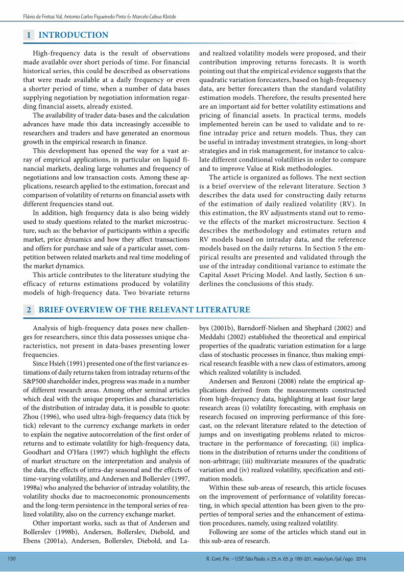
Figure 1 shows that the realized volatilities of the shares analyzed possess significant serial autocorrelation.

RVt,MAq = RVt,u 3.2

^(1- θ1 - ... - θq )

2^

1+ θ12 + ... + θq

2^ ^

Figure 1 Autocorrelation of the PETR4 and VALE5 Realized Volatilities

Table 1 shows the descriptive statistics for the daily re-turns and for the estimated daily RV using the 5 minute grid. There is a certain bias in the non-adjusted RV. Follo-wing the analysis of the daily RV correlograms and the cri-terion adopted by Maheu and McCurdy (2011) to remove

this bias, an MA process with 8 gaps (q=8) appears necessa-ry for the PETR4 returns, while q=11 is appropriate for the VALE5 returns. From here on, RVt = RVt, MAq will be used with q=8 and q=11 for the estimations, respectively, of PE-TR4 and VALE5.

Table 1 Summary statistics: daily returns and realized volatilities

Mean Variance Skewness Kurtosis Minimum Maximum

PETR4

rt -0.090 3.121 -0.404 1.359 -7.596 5.328

RVu 3.155 11.124 4.580 28.561 0.417 32.743

RVma1 0.629 0.443 4.580 28.561 0.083 6.532

RVma2 0.023 0.001 4.580 28.561 0.003 0.237

RVma3 0.083 0.008 4.580 28.561 0.011 0.863

RVma4 0.083 0.008 4.580 28.561 0.011 0.863

RVma4 0.330 0.121 4.580 28.561 0.044 3.420

RVma5 1.031 1.188 4.580 28.561 0.136 10.699

RVma6 1.746 3.405 4.580 28.561 0.231 18.115

RVma7 2.223 5.521 4.580 28.561 0.294 23.067

RVma8 3.083 10.624 4.580 28.561 0.408 31.999

RVma9 3.645 14.844 4.580 28.561 0.482 37.823

RVma10 0.083 0.008 4.580 28.561 0.011 0.863

RVma10 3.951 17.443 4.580 28.561 0.522 41.001

continuous

1.0

0.5

0.0

-0.5

-1.0

Lag Number

ACF

1 3 5 7 9 11 13 15 17 19 21 23 25 27 29 31 33 35 1 3 5 7 9 11 13 15 17 19 21 23 25 27 29 31 33 35

1.0

0.5

0.0

-0.5

-1.0

ACF

Coefficient Upper Confidence Limit Lower Confidence Limit

Lag Number

Realized Volatility - PETR4 Realized Volatility - VALE5



Mean Variance Skewness Kurtosis Minimum Maximum

VALE5

rt -0.011 3.015 -0.364 3.009 -9.958 5.815

RVu 2.866 14.783 6.344 56.496 0.303 46.845

RVma1 0.967 1.684 6.344 56.496 0.102 15.812

RVma2 0.166 0.050 6.344 56.496 0.018 2.717

RVma3 0.000 0.000 6.344 56.496 0.000 0.001

RVma4 0.204 0.075 6.344 56.496 0.022 3.328

RVma5 0.499 0.448 6.344 56.496 0.053 8.155

RVma6 0.646 0.750 6.344 56.496 0.068 10.555

RVma7 0.699 0.879 6.344 56.496 0.074 11.421

RVma8 1.568 4.427 6.344 56.496 0.166 25.635

RVma9 1.646 4.878 6.344 56.496 0.174 26.908

RVma10 1.830 6.029 6.344 56.496 0.193 29.917

RVma11 3.016 16.374 6.344 56.496 0.319 49.302

RVma12 3.468 21.650 6.344 56.496 0.367 56.691

continued

4 METHodoloGy

In this article, bivariate models were proposed ba-sed on two alternative ways in which the RV is related to the conditional variance of returns and the GARCH family models are the reference for performance analy-sis of intraday models.

As in Maheu and McCurdy (2011), two functional forms were proposed for the bivariate models of the returns and the RV. The first model uses the hetero-geneous autoregressive (HAR) function of the lagged log(RV) (Corsi, 2009; Andersen, Bollerslev, & Diebold, 2007). The second model allows the components of the log(RV) to have different decay ratios (Maheu and Mc-Curdy, 2007).

A way to connect the RV to the returns variance was also considered, imposing the restriction that the conditio-nal variance of the daily returns be equal to the conditional expectation of the daily RV.

As with EGARCH and TGARCH models, bivariate models allow the so called leverage effect, or asymme-tries, of the negative innovations versus the positive in-novations of the returns.

One way to confirm that the intraday information con-tributes to the improvement of the estimations of the re-turns distributions is to compare the estimates of the bi-variate models of the return and log(RV) specified in the estimates of the GARCH family models:

GARCH: σ2t = ω + β σ2

t-1 + αe2t-1 4.2

EGARCH: 4.3log (σ2t) = ω + βlog(σ2

t-1) + γ +αet-1σt-1

et-1σt-1

TGARCH: σ2t = ω + β σ2

t-1 + αe2t-1 + γe2

t-1 It-1 where It = 0 if et < 0 and 0 otherwise 4.4

rt = ρ1rt-1 + ρ2rt-2 + θ1et-1 + θ2et-2 + et , et = σt ut, ut ~ NID (0,1) 4.1

The main comparison method implemented uses the root mean squared errors and the Modified Diebold and Mariano (1995) test, based on the work of Harvey, Ley-bourne, and Newbold (1997). Intuitively, better estimated models will have less forecast errors and, if compared with the other inferior performance models, will present statis-tical differences in their errors. Therefore, to assess the mo-dels implemented in this article, we focused on the relative accuracy of those models when estimating the in-sample and the out-of-sample returns.

One important aspect of the approach used is the pos-sibility to directly compare traditional volatility specifica-tions, such as GARCH family models, with the bivariate returns models and RV, because the implemented models possess one common criterion – returns forecast. The ave-rage and the statistical test of these forecast errors allow us to investigate the relative contribution of the RV in the fo-recasts.

4.1 Bivariate Returns Models and Realized Variance.

In this subsection, two combined specifications of the daily return and the RV were implemented. These bivariate models are differentiated by their alternative conditions over the RV dynamic. In each case, restrictions between the equa-tions connect the returns variance to the RV specification.

The corollary one of Andersen et al. (2003) shows that, in realistic empirical conditions, the conditional expecta-tion of the quadratic variation (QVt) is equal to the condi-tional variance of the returns, i.e., Et-1 (QVt) = Vart-1 (rt) σt

2. If the RV is a non-biased estimator of quadratic variation, it follows that the conditional variance of the returns can be linked to RV as σt

2 = Et-1 (RVt), where the combination of information is defined as øt-1 {rt-1, RVt-1, rt-2, RVt-2, ... r1, RV1}.



Supposing that RV possesses a log-normal distribution, the restriction takes on the form:

4.1.1 Heterogeneousauto-regressivespecification:HAR Model.

The first model implemented possesses a bivariate spe-cification for the daily returns and RV in which the con-ditional returns are driven by normal innovations and the dynamic of log (RVt) is captured by a heterogeneous au-toregressive function (HAR) of the lagged log (RVt). Corsi (2009) and Andersen et al. (2007) use the HAR functions aiming to capture the dependence of long-term memory parsimoniously. Motivated by these studies, we defined:

For example, (RVt-22,22) is estimated calculating the ave-rage of log (RV) for the last 22 days, i.e., from t-22 to t-1, log(RVt-5,5) considers the average of the last five days.

This takes the specification of the daily returns and RV with the dynamic of log(RVt) being modeled as an asym-metrical HAR function of the past log(RV)1. This bivariate system is summed up as follows:

This bivariate specification of the daily returns and RV imposes the restriction equation that relates the conditio-nal variance of daily returns with the conditional expecta-tion of daily RV, as shown in (4.5).

Since the data-base analyzed in this article is that of shares returns, it is important to allow asymmetrical effects into the volatility. To facilitate comparisons with the EGARCH reference model, the parameterization in equation (4.8) includes the asymmetric term γet-1 asso-ciated with the innovations of the et-1 returns. The im-pact coefficient for negative innovations of the returns will be γ. Typically, γ < 0, which means the negative innovations of returns imply larger conditional varian-ce for the next period.

4.1.2 Component-Log(RV)Specification:2–CompModel.

This bivariate specification for daily returns and RV possesses conditional returns guided by normal inno-vations, but the dynamic of log(RV) is captured by two components (2-Comp) with a different decay ratio, as shown in Maheu and McCurdy (2007). In particular, this bivariate system can be represented in the equa-tion:

σt2 = Et-1 (RVt) = exp (Et-1 log(RVt) + Vart-1(log(RVt)) 4.51

2

log(RVt-1,1) log(RVt-1) 4.6

log(RVt-h,h) Σ log(RVt-h+i)1h

h-1

i=0

1 The temporal RV series for the assets used here are stationary according to the unit root test, which rejects the null hypothesis of non-stationarity.


log (RVt) = ω + ø1 log (RVt-1) + ø2 log (RVt-5) + ø3 log (RVt-22) + γet-1 + ηvt, vt ~ NID (0,1) 4.8

Again, a restriction was imposed by equation (4.5) whi-ch related the conditional variance of the daily returns with the conditional expectation of the daily RV. For this specifi-cation, the dynamic of daily log(RV) was parameterized by equations (4.10) and (4.11), substituting the HAR function in equation (4.8).

The average of the return time series was estimated by ARMA (p, q) models, using the R software func-tion auto.arima. All other estimates were made using the software eviews 7.1. Aiming to combine parsimony and robustness of these estimates, we established the maximum lag length (p+q) of 4 and automatic lag leng-th selection using the Schwarz Information Criterion (BIC). Thus, for the average of the series we have an AR (1) modeling the daily and weekly series of VALE5 and PETR4 and an ARMA (2,2) for weekly and monthly se-ries of both assets.

The bivariate systems were estimated in two steps. Ini-tially the equations of means were estimated and then the return innovations were modeled by different volatility models.

Volatility forecasts were made by a sequence of one-step ahead forecasts, using the current values for lagged depen-ded variable and return forecasts considering ri,t = fi,t + ei,t, ei,t = σi,t ut, ut ~ NID(0,1) where fi,t is the estimated equation for the mean process for asset i in time t, ei,t is the return innovation for the asset i in time t and αi,t is the estimated conditional standard deviation for the asset i in time t.

Aiming to do a practical exercise for the applicabi-lity of the models presented here, we use the conditio-nal variance estimated by the monthly 2-Comp model, which returned the lowest error predictions among analyzed models, in the Capital Asset Pricing Model – CAPM estimation. The CAPM developed by Sharpe (1964), Treynor (1961), Lintner (1965) and Black, Jen-sen, and Scholes (1972) has become in recent decades the most widespread model for determination of asset prices (Barros, Famá, & Silveira, 2002). This model sta-tes that assets are priced compatible with a trade-off between non-diversifiable risk and expectations of re-turn.

The CAPM can be formally presented as E(ri) = rf + βi (E(rm) - rf) where E(ri) is the expected return on asset i over a single time-period, rf is the riskless rate of interest rate over the period, E(rm) is the expected return on the market over the period, and identifies the exposure of asset i to the market.

To estimate β we used: (i) the statistical covariance Cov (rm, ri) of PETR4 and VALE5 regarding BOVA11 in a mo-


2

i=1log (RVt) = ω + Σ ø1 si,t + γet-1 + ηvt , vt ~ NID (0,1) 4.10

si,t = (1-αi )log (RVt-1) + αi si,t-1 , 0 < αi ,t <1 , i=1,2 4.11

Cov (rm, ri)σ2 (rm)

β =

~



ving window of 22 days and (ii) the conditional variance σ2(rm) estimated by the 2-Comp model in this same time frame. The Interbank Certificate of Deposits - CDI was se-lected to represent the risk free interest rate risk, following the work of Barros, Famá, and Silveira (2002).

To represent the market portfolio, we choose the ex-change traded fund BOVA11, considering that its expected return for the next period is a function of the preceding

2 Bovespa Index (Ibovespa) is the most important indicator of average prices of shares traded on the São Paulo Stock Exchange and it is made up of stocks with the highest trading volume in recent months.

period return. Among the qualities of BOVA11 we have: (i) it is effectively traded in an active market, enabling the extraction of realized volatility and its use in intraday vola-tility models, (ii) it has an average correlation of more than 99% with the Ibovespa2 in the analyzed period, (iii) it is an asset with increasing liquidity, with average daily turnover of R$44.1mi in 2011, and by far the most traded ETF in the Brazilian market.

5 EMpIRICAl RESulTS

In this chapter, we will present the estimated results of models for the 1, 5 and 22 day time models.

Table 2 presents estimates of the GARCH family mo-dels. The Schwarz Information Criterion (BIC) indicates that asymetric models are as well adjusted to the data as the estimated GARCH model, which was confirmed in

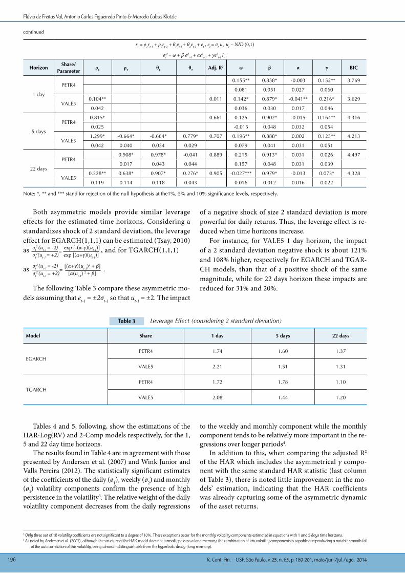
Table 2 GARCH, EGARCH and TGARCH model estimates

rt = ρ1rt-1 + ρ2rt-2 + θ1et-1 + θ2et-2 + et , et = σt ut, ut ~ NID (0,1)

σt2

= ω + β σ2t-1 + αe2

t-1

HorizonShare/

Parameterρ1 ρ2 θ1 θ2 Adj. R2 ω β α γ BIC

1 day

PETR40.159*** 0.883* 0.07** 3.774

0.090 0.060 0.030

VALE50.104** 0.011 0.165** 0.835* 0.096* 3.668

0.042 0.072 0.057 0.034

5 days

PETR40.815* 0.661 0.243 0.849* 0.099** 4.325

0.025 0.153 0.068 0.046

VALE51.299* -0.664* -0.664* 0.779* 0.707 0.211*** 0.856* 0.092** 4.222

0.042 0.040 0.034 0.029 0.118 0.057 0.039

22 days

PETR40.908* 0.978* -0.041 0.889 0.285 0.892* 0.053** 4.483

0.017 0.043 0.044 0.215 0.062 0.029

VALE50.228** 0.638* 0.907* 0.276* 0.905 0.019 0.948* 0.047* 4.325

0.119 0.114 0.118 0.043 0.032 0.021 0.018


HorizonShare/


1 day

PETR4-0.051 0.9405* 0.115** -0.138* 3.778

0.044 0.033 58.000 0.041

VALE50.104** 0.011 -0.005 0.904* 0.101** -0.183* 3.637

0.042 0.032 0.022 0.044 0.037

5 days

PETR40.815* 0.661 -0.070 0.971* 0.1314** -0.118* 4.325

0.025 0.044 0.022 0.059 0.034

VALE51.299* -0.664* -0.664* 0.779* 0.707 -0.032 0.937* 0.145** -0.091* 4.221

0.042 0.040 0.034 0.029 0.039 0.026 0.059 0.036

22 days

PETR40.908* 0.978* -0.041 0.889 0.613 0.496*** 0.245** -0.078 4.499

0.017 0.043 0.044 0.429 0.287 0.111 0.073

VALE50.228** 0.638* 0.907* 0.276* 0.905 -0.069* 1.003* 0.078* -0.045** 4.329

0.119 0.114 0.118 0.043 0.021 0.005 0.028 0.020

nearly all the in sample forecasts of these models. Based on fitted EGARCH and TGARCH models, aside from the monthly estimate of PETR4, all leverage effect coe-fficients are significant at the 10% level, confirming the asymmetrical impact between the positive and negative returns of assets.

continuous

log (σt2) = ω + βlog(σ2

t-1) + γ + αet-1

σt-1

et-1

σt-1



continued


σt2

= ω + β σ2t-1 + αe2

t-1 + γe2t-1 It-1

HorizonShare/


1 day

PETR40.155** 0.858* -0.003 0.152** 3.769

0.081 0.051 0.027 0.060

VALE50.104** 0.011 0.142* 0.879* -0.041** 0.216* 3.629

0.042 0.036 0.030 0.017 0.046

5 days

PETR40.815* 0.661 0.125 0.902* -0.015 0.164** 4.316

0.025 -0.015 0.048 0.032 0.054

VALE51.299* -0.664* -0.664* 0.779* 0.707 0.196** 0.888* 0.002 0.123** 4.213

0.042 0.040 0.034 0.029 0.079 0.041 0.031 0.051

22 days

PETR40.908* 0.978* -0.041 0.889 0.215 0.913* 0.031 0.026 4.497

0.017 0.043 0.044 0.157 0.048 0.031 0.039

VALE50.228** 0.638* 0.907* 0.276* 0.905 -0.027*** 0.979* -0.013 0.073* 4.328

0.119 0.114 0.118 0.043 0.016 0.012 0.016 0.022

Note: *, ** and *** stand for rejection of the null hypothesis at the1%, 5% and 10% significance levels, respectively.

Both asymmetric models provide similar leverage effects for the estimated time horizons. Considering a standardizes shock of 2 standard deviation, the leverage effect for EGARCH(1,1,1) can be estimated (Tsay, 2010) as , and for TGARCH(1,1,1)

as .

The following Table 3 compare these asymmetric mo-dels assuming that et-1 = ±2σt-1 so that ut-1 = ±2. The impact

σt2

(ut-1 = -2) exp [-(α-γ)(ut-1)]σt

2(ut-1 = +2) exp [(α+γ)(ut-1)]=

σt2

(ut-1 = -2) [(α+γ)(ut-1)2 + β]

σt2

(ut-1 = +2) [α(ut-1) 2 + β]=

Table 3 Leverage Effect (considering 2 standard deviation)

Model Share 1 day 5 days 22 days

EGARCHPETR4 1.74 1.60 1.37

VALE5 2.21 1.51 1.31

TGARCHPETR4 1.72 1.78 1.10

VALE5 2.08 1.44 1.20

Tables 4 and 5, following, show the estimations of the HAR-Log(RV) and 2-Comp models respectively, for the 1, 5 and 22 day time horizons.

The results found in Table 4 are in agreement with those presented by Andersen et al. (2007) and Wink Junior and Valls Pereira (2012). The statistically significant estimates of the coefficients of the daily (ø1), weekly (ø2) and monthly (ø3) volatility components confirm the presence of high persistence in the volatility3. The relative weight of the daily volatility component decreases from the daily regressions

to the weekly and monthly component while the monthly component tends to be relatively more important in the re-gressions over longer periods4.

In addition to this, when comparing the adjusted R2 of the HAR which includes the asymmetrical γ compo-nent with the same standard HAR statistic (last column of Table 3), there is noted little improvement in the mo-dels’ estimation, indicating that the HAR coefficients was already capturing some of the asymmetric dynamic of the asset returns.

of a negative shock of size 2 standard deviation is more powerful for daily returns. Thus, the leverage effect is re-duced when time horizons increase.

For instance, for VALE5 1 day horizon, the impact of a 2 standard deviation negative shock is about 121% and 108% higher, respectively for EGARCH and TGAR-CH models, than that of a positive shock of the same magnitude, while for 22 days horizon these impacts are reduced for 31% and 20%.

3 Only three out of 18 volatility coefficients are not significant to a degree of 10%. These exceptions occur for the monthly volatility components estimated in equations with 1 and 5 days time horizons.4 As noted by Andersen et al. (2007), although the structure of the HAR model does not formally possess a long memory, the combination of few volatility components is capable of reproducing a notable smooth fall

of the autocorrelation of this volatility, being almost indistinguishable from the hyperbolic decay (long memory).



Table 4 HAR-log(RV) model estimates


log (RVt) = ω + ø1 log (RVt-1) + ø2 log (RVt-5) + ø3 log (RVt-22) + γet-1 + ηvt, vt ~ NID (0,1)

HorizonShare/

Parameterρ1 ρ2 θ1 θ2 Adj. R2 ω ø1 ø2 ø3 γ η Adj. R2

j Adj. R2

1 day

PETR4- - - - - 0.156** 0.290* 0.345* 0.093 -0.038** -0.021 0.3354 0.3310

- - - - - 0.064 0.060 0.091 0.090 0.017 0.026

VALE50.104** - - - 0.011 0.057 0.312* 0.220** 0.267* -0.058* -0.018 0.3891 0.3753

0.042 - - - 0.055 0.060 0.089 0.088 0.019 0.027

5 days

PETR40.815* 0.661 0.053* 0.113* 0.855* -0.016 -0.011* -0.001 0.9049 0.9040

0.025 0.019 0.018 0.028 0.028 0.004 0.008

VALE51.299* -0.664* -0.664* 0.779* 0.707 0.037** 0.138* 0.807* 0.022 -0.002 -0.007 0.8991 0.8990

0.042 0.040 0.034 0.029 0.019 0.020 0.030 0.030 0.005 0.009

22 days

PETR40.908* 0.978* -0.041 0.889 0.004 0.018* 0.039* 0.944* -0.001 0.001 0.9859 0.9859

0.017 0.043 0.044 0.006 0.006 0.009 0.008 0.001 0.002

VALE50.228** 0.638* 0.907* 0.276* 0.905 0.005 0.014* 0.0036* 0.949* -0.004* -0.002 0.9891 0.9888

0.119 0.114 0.118 0.043 0.005 0.005 0.008 0.008 0.001 0.002


However, the results presented in Table 5 show that the estimated 2-Comp model was able to efficiently capture the different volatility dynamics, with the per-sistent coefficients α1 and α2 clearly differentiated by each time horizon (see Figure 2). In addition to this, the minor α coefficient in each equation shows less persistent effect, being more influenced by the more

recent RV observations.Thus, as in the HAR model that was used, the asym-

metric γ components of the 2-Comp model are negati-ve but also relatively very small, indicating that these models without γ are also able to partially capture the asymmetric balance of the returns.

Table 5 2-Comp model estimates


log (RVt) = ω + Σ ø1 si,t + γet-1 + ηvt , vt ~ NID (0,1)

si,t = (1-αi )log (RVt-1) + αi si,t-1 , 0 < αi ,t <1 , i=1,2

HorizonShare/

Parameterρ1 ρ2 θ1 θ2 Adj. R2 ω ø1 ø2 α1 α2 γ η

1 day

PETR40.071* 0.544* 0.242* 0.784 0.001 -0.017** -0.007

0.023 0.093 0.064 0.007 0.011

VALE50.104** 0.011 0.034 0.516* 0.345* 0.408 0.904 -0.027* -0.006

0.042 0.022 0.076 0.107 0.008 0.011

5 days

PETR40.815* 0.661 0.027* 1.505* -0.579* 0.003 0.354 -0.005* -0.002

0.025 0.007 0.122 0.125 0.002 0.003

VALE51.299* -0.664* -0.664* 0.779* 0.707 0.024* -0.507* 1.432* 0.349 0.018 -0.003 -0.004

0.042 0.040 0.034 0.029 0.007 0.138 0.135 0.002 0.004

22 days

PETR40.908* 0.978* -0.041 0.889 0.009* -0.222* 1.199* 0.770 0.001 -0.001 -0.001

0.017 0.043 0.044 0.002 0.026 0.025 0.001 0.001

VALE50.228** 0.638* 0.907* 0.276* 0.905 0.006* -0.307* 1.291* 0.628 0.001 -0.002* -0.001

0.119 0.114 0.118 0.043 0.002 0.034 0.033 0.000 0.001


2

i=1



Figure 2 presents the graphs of the historical s1,t and s2,t series, generated by the decline of factors α1 and α2 (graph 2.1) and realized and estimated Log(RV) (graph 2.2) for VALE5 in the one day time horizon.

Figure 2 Decay factors and realized and estimated log(RV) for VALE5

In order to assess the accuracy of the models used, they were assessed for the forecast of the following 1, 5 and 22 day time horizons, in and out-of-sample, using the root mean squared error (RMSQ) measure. The Modified Die-bold Mariano test was used5 to estimate the statistical diffe-rences between the models.

For the in-sample period, data collected between 01/07/2010 and 7/29/2011 was considered (388 observa-tions) and for the out-of-sample, data between 08/01/2011

and 03/21/2012 (160 observations).Table 6 presents the RMSQ of the forecasts in the

three defined time horizons. The 2-Comp model re-turned better forecasts for all time horizons, and HAR returned the second best forecast for the 5 and 22 day horizons. But are these results statistically better than the GARCH family models? Table 7 tries to answer these and other questions.

5 This statistical test consists of testing the null hypothesis of equality between the quadratic error mean of two forecasts, using the critical values of a t-Student distribution with (n-1) degrees of liberty.

Table 6 Root mean squared error

In-sample

Horizon Model GARCH EGARCH TGARCH HAR-log(RV) 2-Comp

1 day

PETR4

2.15 2.16 2.16 2.19 1.91

5 days 2.88 2.89 2.87 2.56 2.34

22 days 3.13 3.13 3.13 2.72 2.49

1 day

VALE5

2.14 2.12 2.14 2.17 1.89

5 days 2.76 2.74 2.76 2.49 2.26

22 days 3.04 3.04 3.03 2.69 2.44

Out-of-sample

Horizon Model GARCH EGARCH HAR-RV HAR-log(RV) 2-Comp

1 day

PETR4

3.07 2.97 3.15 3.02 2.59

5 days 4.55 4.31 4.55 3.85 3.44

22 days 4.19 4.00 4.20 3.80 3.42

1 day

VALE5

3.14 3.06 3.37 3.19 2.63

5 days 3.85 3.80 3.98 3.58 3.09

22 days 4.40 4.32 4.47 3.91 3.49

Table 7 shows the p-values of the Modified Diebold Ma-riano Statistical Test.

Regarding the return forecasts in both in and out of

the sample periods, the p-values show that: (i) 2-Comp model provides the best forecasts in the three time ho-rizons; (ii) HAR model has the second best prediction

Fig. 2.1 - S1 and S2 estimated series for VALE5 in 1 day horizon Fig. 2.2 - Realized and Estimated log(RV) for VALE5 in 1 day horizon

1.6

1.2

0.8

0.4

0.0

-0.4

2.0

1.6

1.2

0.8

0.4

0.0

-0.4

-0.8Aug. Sep. Oct. Nov. Dec. Jan. Feb. Mar.

2011 2012

Daily S1Daily S2

Realized log(RV)Estimated log(RV)

Aug. Sep. Oct. Nov. Dec. Jan. Feb. Mar.2011 2012



for the 5 and 22 day horizons. Considering the return forecasts in the sample pe-

riod: (i) there is no significant difference between the GARCH, EGARCH and HAR models in one day time horizon; (ii) there is no significant difference between the GARCH family models in 5 and 22 day time hori-zons.

Furthermore, return forecasts only in the out of the sample period show: (i) in one day time horizon: TGARCH not kept the EGARCH performance, vis a vis

Table 7 Modified Diebold Mariano test (P-Value)

7.1 In-sample 7.2 Out-of-sample

1 day horizon 1 day horizon

GARCH EGARCH TGARCH HAR-RV (log) 2-Comp GARCH EGARCH TGARCH HAR-VR (log) 2-Comp

GARCH

PETR4

100.0% 94.4% 96.9% 67.2% 3.8% GARCH

PETR4

100.0% 8.7% 3.3% 11.6% 0.0%

EGARCH 100.0% 99.4% 81.0% 0.4% EGARCH 100.0% 0.0% 9.9% 0.0%

TGARCH 100.0% 77.0% 0.8% TGARCH 100.0% 0.0% 0.0%

HAR-RV(log) 100.0% 0.0% HAR-RV 100.0% 0.0%

2-Comp 100.0% 2-Comp 100.0%

GARCH

VALE5

100.0% 82.1% 96.3% 74.6% 0.2% GARCH

VALE5

100.0% 7.5% 0.0% 2.5% 0.0%

EGARCH 100.0% 91.6% 52.8% 0.4% EGARCH 100.0% 0.0% 0.0% 0.0%

TGARCH 100.0% 74.0.0% 0.0% TGARCH 100.0% 0.0% 0.0%

HAR-RV(log) 100.0% 0.0% HAR-RV(log) 100.0% 0.0%

2-Comp 100.0% 2-Comp 100.0%

5 days horizon 5 days horizon

GARCH

PETR4

100.0% 85.0% 95.4% 0.0% 0.0% GARCH

PETR4

100.0% 0.0% 57.4% 0.0% 0.0%

EGARCH 100.0% 93.2% 0.0% 0.0% EGARCH 100.0% 0.0% 0.0% 0.0%

TGARCH 100.0% 0.0% 0.0% TGARCH 100.0% 0.0% 0.0%


2-Comp 100.0% 2-Comp 100.0%

GARCH

VALE5

100.0% 80.3% 93.2% 0.0% 0.0% GARCH

VALE5

100.0% 32.6% 0.0% 0.0% 0.0%

EGARCH 100.0% 93.0% 0.0% 0.0% EGARCH 100.0% 0.0% 0.0% 0.0%

TGARCH 100.0% 0.0% 0.0% TGARCH 100.0% 0.0% 0.0%


2-Comp 100.0% 2-Comp 100.0%

22 days horizon 22 days horizon

GARCH

PETR4

100.0% 95.1% 99.4% 0.0% 0.0% GARCH

PETR4

100.0% 0.0% 91.7% 0.0% 0.0%

EGARCH 100.0% 97.3% 0.0% 0.0% EGARCH 100.0% 0.0% 0.0% 0.0%

TGARCH 100.0% 0.0% 0.0% TGARCH 100.0% 0.0% 0.0%


2-Comp 100.0% 2-Comp 100.0%

GARCH

VALE5

100.0% 93.5% 89.8% 0.0% 0.0% GARCH

VALE5

100.0% 0.9% 1.5% 0.0% 0.0%

EGARCH 100.0% 97.2% 0.0% 0.0% EGARCH 100.0% 0.0% 0.0% 0.0%

TGARCH 100.0% 0.0% 0.0% TGARCH 100.0% 0.0% 0.0%


2-Comp 100.0% 2-Comp 100.0%

the similar in sample forecasts of both models; GAR-CH and EGARCH return better predictions than HAR model for VALE5; there are no significant forecast di-fferences of HAR, GARCH and EGARCH models for PETR4; (ii) in the 5 day time horizon, the EGARCH model returns better predictions than TGARCH mo-del; (iii) in the 22 day time horizon, the EGARCH mo-del returns better predictions than the GARCH and TGARCH models.



Figure 3 represents the graphs for the two best out-of-sample forecasts for the PETR4 and VALE5 shares for the three time horizons. It can be observed that the high-frequency models implemented here present very

similar forecasts among themselves. In addition, these forecasts appear to be strongly adherent to the realized returns in all analyzed time horizons.

Figure 3 Realized returns and out-of-sample forecast by the HAR-Log(RV) and 2-Comp models

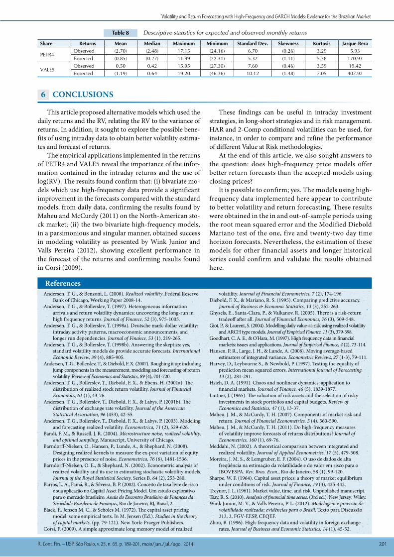
Considering CAPM results, Figure 4 shows the behavior of estimated expected returns series and PE-TR4 and VALE5 return series for the 22 days time hori-

zon. There is a high adherence of the estimated returns to realized returns, with a correlation of 65% and 90%, respectively, for PETR4 VALE5.

Figure 4 Expected and observed monthly returns for PETR4 and VALE5

The following table summarizes the descriptive statis-tics for expected and observed monthly returns of PETR4 and VALE5. We can mention among the results that: (i) the distribution of the expected returns of both shares are

asymmetric to the left and exhibit more fat tails (more lep-tokurtic) than the realized returns and (iii) distributions of the realized and the estimated returns are not normal at the 5% level of significance.

20

10

0

-10

-20

-30Aug. Sep. Oct. Nov. Dec. Jan. Feb. Mar.

2011 2012

Observed Weekly Return - PETR42-Comp Weekly Return - PETR4HAR Weekly Return - PETR4

Aug. Sep. Oct. Nov. Dec. Jan. Feb. Mar.2011 2012

Observed Monthly Return - PETR42-Comp Monthly Return - PETR4HAR Monthly Return - PETR4

15

10

5

0

-5

-10

-15

-20

-25


2011 2012

Observed Weekly Return - VALE52-Comp Weekly Return - VALE5HAR Weekly Return - VALE5

20

10

0

-10

-20


2011 2012

Observed Monthly Return - VALE52-Comp Monthly Return - VALE5HAR Monthly Return - VALE5

30

20

10

0

-10

-20

-30

20

10

0

-10

-20

-30

20

10

0

-10

-20

-30

-40

-50Jan. Apr. Jul. Oct. Jan. Apr. Jul.

2010 2011

Observed montly return - PETR4Expected montly return - PETR4

Observed montly return - VALE5Expected montly return - VALE5

Jan. Apr. Jul. Oct. Jan. Apr. Jul.2010 2011



Table 8 Descriptive statistics for expected and observed monthly returns

Share Returns Mean Median Maximum Minimum Standard Dev. Skewness Kurtosis Jarque-Bera

PETR4Observed (2.70) (2.48) 17.15 (24.16) 6.70 (0.26) 3.29 5.93Expected (0.85) (0.27) 11.99 (22.31) 5.32 (1.11) 5.38 170.93

VALE5Observed 0.50 0.42 15.95 (27.30) 7.60 (0.46) 3.59 19.42Expected (1.19) 0.64 19.20 (46.36) 10.12 (1.48) 7.05 407.92

6 ConCluSIonS

This article proposed alternative models which used the daily returns and the RV, relating the RV to the variance of returns. In addition, it sought to explore the possible bene-fits of using intraday data to obtain better volatility estima-tes and forecast of returns.

The empirical applications implemented in the returns of PETR4 and VALE5 reveal the importance of the infor-mation contained in the intraday returns and the use of log(RV). The results found confirm that: (i) bivariate mo-dels which use high-frequency data provide a significant improvement in the forecasts compared with the standard models, from daily data, confirming the results found by Maheu and McCurdy (2011) on the North-American sto-ck market; (ii) the two bivariate high-frequency models, in a parsimonious and singular manner, obtained success in modeling volatility as presented by Wink Junior and Valls Pereira (2012), showing excellent performance in the forecast of the returns and confirming results found in Corsi (2009).

These findings can be useful in intraday investment strategies, in long-short strategies and in risk management. HAR and 2-Comp conditional volatilities can be used, for instance, in order to compare and refine the performance of different Value at Risk methodologies.

At the end of this article, we also sought answers to the question: does high-frequency price models offer better return forecasts than the accepted models using closing prices?

It is possible to confirm; yes. The models using high-frequency data implemented here appear to contribute to better volatility and return forecasting. These results were obtained in the in and out-of-sample periods using the root mean squared error and the Modified Diebold Mariano test of the one, five and twenty-two day time horizon forecasts. Nevertheless, the estimation of these models for other financial assets and longer historical series could confirm and validate the results obtained here.

Andersen, T. G., & Benzoni, L. (2008). Realized volatility. Federal Reserve Bank of Chicago, Working Paper 2008-14.

Andersen, T. G., & Bollerslev, T. (1997). Heterogeneous information arrivals and return volatility dynamics: uncovering the long-run in high frequency returns. Journal of Finance, 52 (3), 975-1005.

Andersen, T. G., & Bollerslev, T. (1998a). Deutsche mark-dollar volatility: intraday activity patterns, macroeconomic announcements, and longer run dependencies. Journal of Finance, 53 (1), 219-265.

Andersen, T. G., & Bollerslev, T. (1998b). Answering the skeptics: yes, standard volatility models do provide accurate forecasts. International Economic Review, 39 (4), 885-905.

Andersen, T. G., Bollerslev, T., & Diebold, F. X. (2007). Roughing it up: including jump components in the measurement, modeling and forecasting of return volatility. Review of Economics and Statistics, 89 (4), 701-720.

Andersen, T. G., Bollerslev, T., Diebold, F. X., & Ebens, H. (2001a). The distribution of realized stock return volatility. Journal of Financial Economics, 61 (1), 43-76.

Andersen, T. G., Bollerslev, T., Diebold, F. X., & Labys, P. (2001b). The distribution of exchange rate volatility. Journal of the American Statistical Association, 96 (453), 42-55.

Andersen, T. G., Bollerslev, T., Diebold, F. X., & Labys, P. (2003). Modeling and forecasting realized volatility. Econometrica, 71 (2), 529-626.

Bandi, F. M., & Russell, J. R. (2004). Microstructure noise, realized volatility, and optimal sampling. Manuscript, University of Chicago.

Barndorff-Nielsen, O., Hansen, P., Lunde, A., & Shephard, N. (2008). Designing realized kernels to measure the ex-post variation of equity prices in the presence of noise. Econometrica, 76 (6), 1481-1536.

Barndorff-Nielsen, O. E., & Shephard, N. (2002). Econometric analysis of realized volatility and its use in estimating stochastic volatility models. Journal of the Royal Statistical Society, Series B, 64 (2), 253-280.

Barros, L. A., Famá, R., & Silveira, B. P. (2002). Conceito de taxa livre de risco e sua aplicação no Capital Asset Pricing Model. Um estudo explorativo para o mercado brasileiro. Anais do Encontro Brasileiro de Finanças da Sociedade Brasileira de Finanças, Rio de Janeiro, RJ, Brasil, 2.

Black, F., Jensen M. C., & Scholes M. (1972). The capital asset pricing model: some empirical tests. In M. Jensen (Ed.). Studies in the theory of capital markets. (pp. 79-121). New York: Praeger Publishers.

Corsi, F. (2009). A simple approximate long memory model of realized

volatility. Journal of Financial Econometrics, 7 (2), 174-196.Diebold, F. X., & Mariano, R. S. (1995). Comparing predictive accuracy.

Journal of Business & Economic Statistics, 13 (3), 252-263.Ghysels, E., Santa-Clara, P., & Valkanov, R. (2005). There is a risk-return

tradeoff after all. Journal of Financial Economics, 76 (3), 509-548.Giot, P., & Laurent, S. (2004). Modelling daily value-at-risk using realized volatility

and ARCH type models. Journal of Empirical Finance, 11 (3), 379-398.Goodhart, C. A. E., & O'Hara, M. (1997). High frequency data in financial

markets: issues and applications. Journal of Empirical Finance, 4 (2), 73-114.Hansen, P. R., Large, J. H., & Lunde, A. (2008). Moving average-based

estimators of integrated variance. Econometric Reviews, 27 (1-3), 79-111.Harvey, D., Leybourne S., & Newbold, P. (1997). Testing the equality of

prediction mean squared errors. International Journal of Forecasting, 13 (2), 281-291.

Hsieh, D. A. (1991). Chaos and nonlinear dynamics: application to financial markets. Journal of Finance, 46 (5), 1839-1877.

Lintner, J. (1965). The valuation of risk assets and the selection of risky investments in stock portfolios and capital budgets. Review of Economics and Statistics, 47 (1), 13-37.

Maheu, J. M., & McCurdy, T. H. (2007). Components of market risk and return. Journal of Financial Econometrics, 5 (4), 560-590.

Maheu, J. M., & McCurdy, T. H. (2011). Do high-frequency measures of volatility improve forecasts of returns distributions? Journal of Econometrics, 160 (1), 69-76.

Meddahi, N. (2002). A theoretical comparison between integrated and realized volatility. Journal of Applied Econometrics, 17 (5), 479-508.

Moreira, J. M. S., & Lemgruber, E. F. (2004). O uso de dados de alta freqüência na estimação da volatilidade e do valor em risco para o IBOVESPA. Rev. Bras. Econ., Rio de Janeiro, 58 (1), 99-120.

Sharpe, W. F. (1964). Capital asset prices: a theory of market equilibrium under conditions of risk. Journal of Finance, 19 (3), 425-442.

Treynor, J. L. (1961). Market value, time, and risk. Unpublished manuscript. Tsay, R. S. (2010). Analysis of financial time series. (3rd ed.). New Jersey: Wiley. Wink Junior, M. V., & Valls Pereira, P. L. (2012). Modelagem e previsão de

volatilidade realizada: evidências para o Brasil. Texto para Discussão 313, 3, FGV-EESP, CEQEF.

Zhou, B. (1996). High-frequency data and volatility in foreign exchange rates. Journal of Business and Economic Statistics, 14 (1), 45-52.

References

issn 1808-057x volatility and return forecasting with high ... · volatility and return forecasting...

Documents