Structural GARCH: The Volatility-Leverage Connection

Robert Engle Emil Siriwardane

Working Paper 16-009

Working Paper 16-009

Copyright © 2015, 2016 by Robert Engle and Emil Siriwardane

Working papers are in draft form. This working paper is distributed for purposes of comment and discussion only. It may not be reproduced without permission of the copyright holder. Copies of working papers are available from the author.

Structural GARCH: The Volatility-Leverage Connection

Robert Engle NYU Stern School of Business

Emil Siriwardane Harvard Business School

Structural GARCH: The Volatility-Leverage

Connection*

Robert Engle† Emil Siriwardane‡

Abstract

During the financial crisis, financial firm leverage and volatility both rose dra-matically. Consequently, institutions are being asked to reduce leverage in orderto reduce risk, though the effectiveness depends upon the role of capital structurein volatility. To address this question, we build a statistical model of equity volatil-ity that accounts for leverage. Our approach blends Merton’s insights on capitalstructure with traditional time-series models of volatility. Using our model wequantify how capital injections impact the risk of financial institutions and es-timate firm specific precautionary capital needs. In addition, the longstandingobservation that volatility is more responsive to negative shocks than positive isshown to be less a consequence of actual leverage than it is of risk premiums.

*We are grateful to Viral Acharya, Rui Albuquerque, Torben Andersen, Tim Bollerslev, Gene Fama,Xavier Gabaix, Paul Glasserman, Lars Hansen, Andrew Karolyi, Bryan Kelly, Andy Lo, Eric Renaultand two anonymous referees for valuable comments and discussions, and to seminar participants atAQR Capital Management, the Banque de France, Duke Economics, ECB MaRS 2014, the Universityof Chicago (Booth), the MFM Fall 2013 Meetings, the Office of Financial Research (OFR), NYU Stern,and the WFA (2014). We also thank Constantin Roth for sharing his data on realized variance, andwe are extremely indebted to Rob Capellini for all of his help on this project. The authors thank-fully acknowledge financial support from the Sloan Foundation. The views expressed in this paperare those of the authors’ and do not necessarily reflect the position of the Office of Financial Re-search (OFR), or the U.S. Treasury Department. The Online Appendix for the paper may be found athttp://www.people.hbs.edu/esiriwardane.

†Engle: NYU Stern School of Business. E-mail: rengle@stern.nyu.edu‡Siriwardane: Harvard Business School. E-mail: esiriwardane@hbs.edu.

1

1 Introduction

The financial crisis revealed the damaging role of financial market leverage on the real

economy. Nonetheless, it is far from clear that reducing this leverage will stabilize the

real economy, let alone stabilize the financial sector. The extreme volatility of asset

prices was a joint consequence of the high impact of economic news and high lever-

age. A critical question that remains is how much reduction in equity volatility could

be expected from reductions in leverage. The answer to this question will imply an

estimate of the capital that a financial firm should have in order to achieve certain

stability targets.

To address this issue, we introduce a statistical model of equity volatility that ac-

counts for capital structure. We do so by incorporating the insight from Merton (1974)

into a GARCH volatility model following Engle (1982) and Bollerslev (1986). In addi-

tion, our model nests models of volatility asymmetry (Nelson (1991); Glosten, Jagan-

nathan, and Runkle (1993)) that have been widely discussed in the intervening years.

Given its theoretical underpinnings, we call this new model Structural GARCH.

The key feature of our Structural GARCH model is that the risk of future equity

returns depends on a firm’s current capital structure. This observation dates back to at

least Modigliani and Miller (1959), but has yet to make its way into the vast literature on

volatility modeling. In our model, unobserved asset returns follow a GARCH process,

and are amplified by what we call a leverage multiplier to generate equity returns. The

leverage multiplier is derived from Merton’s observation that equity is a call option on

the underlying assets of the firm with a strike price that is the face value of the liabilities

and a maturity given by the due date of the liabilities. Under reasonable assumptions,

the leverage multiplier becomes a simple function of observable leverage, and its exact

functional form depends on easily estimated parameters.

We estimate the Structural GARCH model for a sample of the one hundred largest

U.S. financial firms. Our empirical results show that incorporating leverage into the

GARCH framework is very useful for capturing the dynamics of financial firm equity

volatility. The Structural GARCH model outperforms a standard GARCH model in a few

ways. First, the Structural GARCH is favored in a statistical sense by a majority of the

firms in our sample. This follows from the fact that our model nests the GARCH family,

and thus provides a straightforward way to assess the statistical significance of leverage

for equity volatility. Second, we compare the ability of the Structural GARCH model

2

to forecast high-frequency realized variance. Compared to the standard GARCH, our

Structural GARCH model is superior for most firms in our sample as well.

Our model delivers estimates of time-varying equity volatility and asset volatility,

as well as the leverage multiplier that links the two. Using these outputs, we start by

decomposing the massive rise in financial sector equity volatility during the financial

crisis, which reached almost 200% in annualized terms. To put this in perspective, the

VIX index reached about 60% during this same time period. During the early phase of

the crisis (May 2007 – Sept 2008), the rise in equity volatility was driven in large part

by a steady increase in the leverage multiplier of the financial sector. At its peak, the

financial sector leverage multiplier hits 20, indicating that asset shocks are amplified

by a factor of 20. In contrast, the rise in financial sector asset volatility did not really

occur until late in 2008.

Next, we use the Structural GARCH model to quantify how capital injections impact

the risk of financial institutions. As a demonstrating example, we put ourselves in the

position of U.S. regulators standing in October 2008 and evaluate the potential impact

of a $25 billion equity injection into Bank of America.1 Unsurprisingly, at all horizons,

adding more capital lowers the volatility of equity returns and reduces the likelihood of

extreme events. According to our model, injecting Bank of America with capital lowers

the probability of going bankrupt over the next month by a factor of nearly three. It

is of course up to the regulator to assess the importance of this effect, and in turn,

how large of a capital injection to require — our model presents a way to quantify this

tradeoff.

Building on this analysis, we then define a new measure of systemic risk for finan-

cial institutions, and we refer to this measure as precautionary capital. Precautionary

capital is the answer to the question: how much equity do we have to add to a firm

today in order to ensure some arbitrary level of confidence that the firm will have ad-

equate capital in a future crisis? The issue of precautionary capital is thus highly re-

lated to the Federal Reserve’s stress testing (CCAR) of U.S. financial institutions. In the

Structural GARCH model, we quantitatively show that preventative measures that re-

duce leverage can be very powerful since holding more capital results in lower volatil-

ity, lower beta, and lower probability of failure. This is a sensible outcome that is not

implied by conventional time-series volatility models because capital structure has no

1This corresponds to the size of the first equity injection BAC would actually receive from the U.S.government.

3

explicit role in determining risk dynamics.

Because our model links leverage and volatility, it also sheds light on the sources of

volatility asymmetry. Volatility asymmetry describes situations where negative equity

returns predict higher future volatility, relative to positive equity returns of the same

magnitude. The original explanation for this phenomenon dates back to Black (1976)

and Christie (1982), who ascribe it to a mechanical leverage effect: declines in equity

today mechanically increase leverage, and because higher leverage is associated with

more risk, future equity volatility also rises. French, Schwert, and Stambaugh (1987)

observe that risk premiums could also account for volatility asymmetry. In their al-

ternative, a rise in future volatility raises the required return on equity, leading to an

immediate decline in the stock price.

One challenge in distinguishing between these two explanations is that asset re-

turns are unobservable, so teasing out the causes of volatility asymmetry typically re-

quires alternative strategies (Duffee (1995); Bekaert and Wu (2000); Choi and Richard-

son (2015)). The Structural GARCH model provides a simple way to estimate asset

returns and volatility, while crucially allowing for the debt of each firm to be risky. We

find that almost all of the volatility asymmetry that is present in equity returns is still

present in asset returns. This cuts strongly against the mechanical leverage effect ex-

planation. We then compute idiosyncratic asset returns by purging asset returns of

exposure to priced risk factors (Fama and French (1993)). In our sample, idiosyncratic

asset returns display very little volatility asymmetry, which lends support to the risk

premium explanation of asymmetry.

Literature Review

At its core, the Structural GARCH is a time-series model of volatility that explicitly al-

lows leverage to impact equity volatility. As the name suggests, the way in which lever-

age interacts with equity volatility is motivated by structural models of credit (Merton

(1974)). A non-exhaustive list of theoretical extensions of the Merton (1974) model

includes Black and Cox (1976), Leland and Toft (1996), and Collin-Dufresne and Gold-

stein (2001). Because our model allows asset volatility to be time-varying, we also con-

nect to variants of the Merton (1974) model with stochastic volatility (e.g. McQuade

(2013), Elkamhi, Ericsson, and Jiang (2011), and Fouque, Sircar, and Sølna (2006)).

The exact stochastic nature of asset returns in our model draws from time-series

4

models of volatility (Engle (1982) and Bollerslev (1986)). Nelson (1991), Glosten, Ja-

gannathan, and Runkle (1993), and Engle and Ng (1993) are notable extensions of the

ARCH/GARCH class that indirectly allow capital structure to impact future volatility.

They do so by allowing negative returns to impact future volatility differently than pos-

itive returns. The basic idea behind these models is that negative shocks to equity raise

leverage and therefore may raise equity risk more than positive shocks of the same

magnitude (so-called “volatility asymmetry”). The Structural GARCH is closely related

to this set of models, but makes an important departure in allowing capital structure

to directly impact volatility dynamics. Intuitively, in our model, the level of leverage

determines the level of equity volatility, while still allowing for volatility asymmetry in

asset returns.2

This approach allows us to disentangle the causes of volatility asymmetry, which

as mentioned dates back to Black (1976), Christie (1982), and French, Schwert, and

Stambaugh (1987). Our main finding is that mechanical leverage drives almost none

of the observed equity volatility asymmetry for the firms in our sample. These results

are consistent with, among others, Bekaert and Wu (2000) and Hasanhodzic and Lo

(2013). Both studies find that leverage does not appear to fully explain the asymmetry

in equity volatility. In contrast to the current paper, Bekaert and Wu (2000) assume

that debt is riskless and are therefore silent about the nonlinear interaction between

equity volatility and leverage. Hasanhodzic and Lo (2013) focus on a subset of firms

with no leverage, which we do not pursue in this paper. Choi and Richardson (2015)

also study volatility asymmetry by invoking the second Modigliani–Miller theorem. In

turn, they directly compute the market value of assets at a monthly frequency by first

constructing a return series for the market value of bonds (and loans). Still, determin-

ing the true market value of the bonds of a given firm is difficult in lieu of liquidity

issues, especially at the daily frequency with which our model operates.

Our paper also connects to a rapidly growing systemic risk literature that empha-

sizes the consequences of undercapitalization of financial institutions. Acharya, Ped-

ersen, Philippon, and Richardson (Forthcoming) develop a model where the social

cost of undercapitalized banks is greater than the private cost. Consequently, there are

incentives to take more leverage and risk than is socially optimal. Acharya, Engle, and

2Carr and Wu (Forthcoming) use this intuition in building a reduced-form model of leverage andequity variance to study the pricing of S&P 500 index options. Geske, Subrahmanyam, and Zhou (2016)also investigate the impact of leverage on option prices using a compound option pricing model.

5

Richardson (2012) and Brownlees and Engle (Forthcoming) develop an econometric

approach to measuring the capital shortfall based on comovements of financial stocks

and the broad market. Other popular measures of fragility are based solely on equity

data such as the CoVaR model of Adrian and Brunnermeier (2016) and the network

models of Billio, Getmansky, Lo, and Pelizzon (2012) and Diebold and Yilmaz (2014).

These academic studies are closely linked to the new developments in macropru-

dential regulation since Dodd Frank and Basel II and III. Following these protocols,

bank stress tests are carried out in order to measure whether banks are sufficiently

well capitalized. There are two risks to be considered when the banking sector as a

whole is undercapitalized. The first is that there will be an exogenous shock that will

be sufficiently large that highly leveraged financial firms will fail and cause a severe

decline in output. The second is that the undercapitalization itself will bring about the

decline. As the entire banking sector tries to reduce its risk by deleveraging, it will drive

down the value of assets that are being sold and create a downward spiral of bank valu-

ations through the fire sale externality. This has been discussed by Brunnermeier and

Pedersen (2009), among others. Typically in stress tests, the regulator will estimate the

capital adequacy ratio under stress and give either a pass or a fail to the bank which

may then have to revise its capital plans. Neither the regulators nor the banks actually

estimate the capital shortfall. Presumably this is because it is difficult to estimate the

impact of changes in capital structure on volatility and on correlation. Thus the model

developed in this paper could assist both regulators and banks in estimating the extent

of capital augmentation needed to pass stress tests.

The remainder of the paper is organized as follows. Section 2 develops our workhorse

econometric model. Section 3 provides details on how we take our model to the data

and analyzes the resulting estimates for our cross section of financial firms. In this

section, we also consider some additional model validation to further emphasize the

importance of accounting for the connection between equity volatility and leverage.

Section 4 presents two applications of our Structural GARCH model: (i) measuring sys-

temic risk and (ii) understanding the cause of volatility asymmetry in equity returns.

Section 5 concludes the paper by suggesting additional uses of our new model.

6

2 The Model

2.1 Motivation

The ARCH/GARCH Framework

Our simple goal is to incorporate capital structure into the ARCH/GARCH class of

volatility models. These models typically take the following form:

rE,t = �E,t ⇥ "E,t

where rE,t denotes demeaned equity returns and "E,t is a mean zero and variance one

shock. �E,t is the conditional volatility of equity returns, and in the standard GARCH

model, it is conditioned on past information information (Ft�1) as follows:

�

2E,t = E

⇥r

2E,t|Ft�1

⇤

= E⇥r

2E,t|rE,t�1,rE,t�2, ...rE,1

⇤

This conditional expectation is typically parametrized as a recursive process �

2E,t =

! + ↵r

2E,t�1 + ��

2E,t�1, though more elaborate recursive structures can be handled

easily. In this paper, we add leverage to the set of conditioning variables:

�

2E,t = E

⇥r

2E,t|Leveraget�1, rE,t�1,rE,t�2, ...rE,1

⇤(1)

The basic logic of our approach is to use structural models of credit to provide eco-

nomic discipline in terms of how we introduce leverage into Equation (1).

Structural Models of Credit

To motivate the economic relationship between leverage and equity volatility, we start

from the observation that a firm’s equity can be viewed as a call option on the under-

lying assets of the firm (Merton (1974)):

Et = f (At, Dt, �A,t, ⌧t, rt;⇥p,⇥r) (2)

where f(·) is an unspecified call option function,At is the current (unobservable) mar-

ket value of assets and Dt is the current book value of outstanding debt, which we in-

7

terpret as the face value of debt. �A,t is the potentially stochastic volatility of the assets,

⌧t is the life of the debt in years, and rt is the annualized risk-free rate at time t. ⇥p is a

vector of parameters that govern the asset dynamics under the physicalP-measure. ⇥r

is a vector of parameters that describe the pricing of risks and derives from the under-

lying preference parameters that enter the stochastic discount factor in the economy.

In Appendix A.1 we argue that Equation (2) implies that equity volatility (under the

P-measure) can be well-approximated as:

�E,t = LM (Dt/Et, �A,t, ⌧t, rt;⇥p,⇥r) ⇥ �A,t (3)

where the function LM(·) is what we call the “leverage multiplier”. To derive this re-

lationship, we assume a generic process for asset returns that nests many popular op-

tion pricing settings from the previous literature.3 We then compute the law of motion

for equity returns using repeated applications of Ito’s Lemma. Finally, we show that

for reasonable parameter values governing asset return dynamics, equity volatility is

a scaled function of asset volatility, where the function depends on financial leverage.

Thus, LM captures how financial leverage amplifies asset volatility to generate equity

volatility. Intuitively, the exact functional form of the leverage multiplier is ultimately

dictated by the specific call option pricing function f(·) from Equation (2); however,

as we show shortly, it has some basic properties that do not appear to depend on the

particular option pricing setting. When it is obvious, we will drop the functional de-

pendence of the leverage multiplier on its arguments and instead denote it simply by

LMt.

Some Examples and Intuition

To develop some intuition of how the leverage multiplier depends on financial lever-

age, Figure 1 plots the leverage multiplier under some different option pricing mod-

els. In particular, we consider three different settings: (i) the Black-Scholes-Merton

(BSM) model; (ii) the Bakshi, Cao, and Chen (1997) model (BCC), which is an exten-

sion of the BSM model that allows for stochastic volatility and jumps; and (iii) a dis-

crete time model where risk-neutral asset returns evolve according to an asymmetric

GARCH process (Glosten, Jagannathan, and Runkle (1993), Barone-Adesi, Engle, and

3A short and certainly incomplete list includes Black and Scholes (1973), Heston (1993), Stein andStein (1991), and Bates (1996).

8

Mancini (2008), Duan (1995)).4 Studying the leverage multiplier in these environments

is useful because they span a variety of assumptions regarding discrete and continu-

ous time, stochastic volatility, and jumps. Appendix B contains additional details on

how we parametrize and compute the leverage multiplier in these different settings.

In all cases, we are measuring leverage as the book value of debt divided by the market

value of equity.

Figure 1 reveals interesting differences in the leverage multiplier across the three

models. For instance, the leverage multiplier in the BCC model is larger than the BSM

multiplier for all values of leverage. This occurs because the BCC asset return process

has jumps that are negative on average, and also because there is a negative correlation

between asset volatility shocks and the Gaussian asset return shocks. The combina-

tion of both forces means that the asset return distribution in the BCC model is more

left skewed compared to the BSM model. In turn, leverage leads to more amplified

equity volatility because high leverage corresponds to a much smaller likelihood the

equity expires “in the money.” A similar intuition holds when looking at the leverage

multiplier when risk-neutral asset returns follow an asymmetric GARCH process. The

way we have parameterized the asymmetric GARCH process in Figure 1 implies that

volatility innovations and asset return innovations are negatively correlated, thereby

leading to a large negative skew in asset returns (Engle (2011)).

On the other hand, Figure 1 also highlights that the leverage multiplier has some

characteristics that are common across the different option pricing models. For one,

when leverage is zero, the leverage multiplier is one. This result is mechanical given

that zero leverage means that the market value of assets is exactly the market value of

equity, so their volatilities have to coincide. A second common feature is that the lever-

age multiplier is monotonically increasing in leverage. Intuitively, as a firm becomes

more leveraged, equity volatility increases for a given level of asset volatility. Finally, in

all three models, the leverage multiplier appears to be concave in leverage. The intu-

ition for this result is less clear, but one way to rationalize the concavity of the leverage

multiplier is to consider a firm with extremely high leverage. In this case, the equity

of the firm is close to worthless, so adding an additional unit of leverage does not add

much more in terms of volatility amplification.5 Motivated by the fact that some char-

4McQuade (2013), Elkamhi, Ericsson, and Jiang (2011), and Fouque, Sircar, and Sølna (2006) are a fewadditional examples of efforts made in the credit risk literature to extend the Merton model to accountfor stochastic volatility.

5We believe that all three of these properties are general features that likely derive from no arbitrage

9

acteristics of the leverage multiplier appear independent of a specific option pricing

model, we now propose a function to capture the leverage amplification mechanism

in a relatively “model-free” way.

2.2 A Flexible Leverage Multiplier

One approach to quantifying how leverage amplifies asset volatility into equity volatil-

ity would be to choose a particular option pricing model, fit the parameters of that

model to observed leverage levels, and then use the estimated parameters to trace out

the leverage multiplier. The downside to this approach is that it forces one to take

a stance on an option pricing model. However, an alternative route that we take is

to model the leverage multiplier directly, without imposing a specific option pricing

model on the data. Specifically, we propose the following function of leverage:

LM

✓Dt

Et

, �A,t, ⌧t, rt;�

◆=

LM

BSM

✓Dt

Et

, �A,t, ⌧t, rt

◆��, � � 0 (4)

where LM

BSM is the leverage multiplier in the Black-Scholes-Merton model. We pro-

vide a more explicit expression for LMBSM in Appendix A.2, as well as additional de-

tails on how to compute it using observed values of leverage.

It is critical to recognize that we are not assuming that the underlying option pric-

ing model is the Black-Scholes-Merton model, and as such, the success of our em-

pirical approach does not rest on the ability of the BSM model as a structural model

of credit. Instead, our leverage multiplier simply uses a mathematical transformation

of the BSM functions. This is captured by the new parameter �, which will be an esti-

mated parameter when we take our model to the data. One advantage of our proposed

leverage multiplier in Equation (4) is its relative simplicity in terms of computation, as

the BSM leverage multiplier is numerically tractable. This specification is also a par-

simonious way to capture some of the features of the leverage multiplier documented

in Section 2.1, while still maintaining some level of agnosticism over the true option

pricing model that drives volatility amplification.6

arguments, similar to those put forth in Merton (1973). While it is straightforward to show this in a givenoption pricing model, we have been unsuccessful in proving this formally.

6To be precise, � preserves the concavity of the leverage multiplier with respect to leverage as long asit is not too large, long-run asset volatility is not too small, and ⌧ is not too small. In practice, this is notan issue. When we estimate the model, we verify that none of the fitted � result in violations of this sort.

10

Figure 2 demonstrates the flexibility of our proposed leverage multiplier. In the

figure, we have reproduced the leverage multipliers from the Bakshi, Cao, and Chen

(1997) and the GARCH models that we explored in the previous subsection. These cor-

respond to the solid lines with square and triangle markers, respectively. In addition,

we have estimated two different values of � in our proposed leverage multiplier to best

match the two models. The leverage multipliers from this exercise are plotted in dotted

lines, and the legend in the figure displays the estimated value of � in both cases. The

simple takeaway from Figure 2 is that toggling � in our proposed function is effective

in replicating the leverage multiplier in both the BCC and GARCH settings, despite the

fact that they have very different features (e.g. jumps, continuous versus discrete time,

etc.).

2.3 The Full Recursive Model

The preceding analysis motivates the use of our leverage multiplier in describing the

relationship between equity volatility and leverage. To make the model fully opera-

tional in discrete time, we propose the following recursive process for equity returns:

rE,t = LMt�1rA,t

rA,t =

phA,t"A,t, "A,t ⇠ D(0, 1)

hA,t = ! + ↵

✓rE,t�1

LMt�2

◆2

+ �

✓rE,t�1

LMt�2

◆2

1rE,t�1<0 + �hA,t�1

LMt�1 =

LM

BSM

✓Dt�1

Et�1, �

⌧A,t�1, ⌧t�1, rt�1

◆��(5)

where "A,t has a mean zero and variance one. We call the specification described in

Equation (5) a “Structural GARCH” model. To see how this model maps to the motiva-

tion in the previous sections, notice that equity variance hE,t is given by:

hE,t = LM

2t�1hA,t

which is exactly the relationship that is implied by structural models of credit (see

Equation (3)). Here, hA,t represents the variance of asset returns, rA,t. It evolves ac-

cording to the volatility model introduced by Glosten, Jagannathan, and Runkle (1993)

(GJR), which is a member of the GARCH family. This is easiest to see by observing that

11

rE,t�1/LMt�2 = rA,t�1, which means that asset variance can be expressed as the more

standard GJR recursion:

hA,t = ! + ↵r

2A,t�1 + �r

2A,t�11rA,t�1 + �hA,t�1

We chose the GJR model for asset variance because it nests a standard GARCH model

(� = 0) and has been shown to display superior performance when applied to equity

returns directly (Engle and Ng (1993)). The GJR formulation for asset variance will also

prove useful when we use the Structural GARCH model to examine volatility asym-

metry in Section 4.2, though a number of alternative volatility models (e.g. Nelson

(1991)) would serve this purpose. The total parameter set for the Structural GARCH

is ⇥ := (!,↵, �, �,�). Importantly, there is only one extra parameter compared to a

simple GJR model, though one could add additional lags and parameters in a natural

way. Also note that we have formulated the Structural GARCH model for an arbitrary

firm, but in our empirical work we will estimate a separate model for each firm in our

sample.

With some abuse of notation, we use �

⌧A,t�1 to denote the expected cumulative as-

set volatility over the life of the debt. This is different than (but highly related to) the

instantaneous volatility of assets hA,t. We will confront the issue of how to compute

⌧t and how to use the volatility input �⌧A,t�1 in the next section when describing the

data and estimation techniques used in our empirical work. We also introduce lags in

the appropriate variables (e.g., the leverage multiplier) to ensure that one-step ahead

volatility forecasts are indeed in the previous day’s information set. An attractive fea-

ture of the model in (5) is that it nests a simple GJR model (� = 0), thus providing a

statistical test of how leverage affects equity volatility.

Additional Discussion

A Feedback Mechanism

Another advantage of our equity volatility model is that it explicitly allows for feedback

between leverage and volatility. For example, when simulating this model, if a series of

negative asset returns is realized (and hence negative equity returns since they share

the same shock), volatility rises more due to the asymmetric specification inherent in

the GJR. Negative equity returns also lead to an increase in leverage, which in turn in-

creases the leverage multiplier and results in an even stronger amplification effect for

12

equity volatility. As we saw in the recent financial crisis, this was a key feature of the

data, particularly for highly leveraged financial firms.

Asset Levels versus Asset Returns

The specification in Equation (5) also suggests that we can recover asset returns as the

ratio of equity returns to the lagged leverage multiplier. However, it is important to

recognize that we are not able to recover the level of the market value of assets. This is

because we have not taken a stand on a particular option pricing model that is driving

the data. Instead, our estimated leverage multiplier tells us how shocks to asset returns

get scaled into equity returns.

Physical Versus Risk-Neutral Volatility

A subtle and perhaps surprising aspect of our model is that it describes asset returns

and volatility under the physical measure, as opposed to the risk neutral measure. At

first glance, this may seem puzzling given that the observed equity values are options

on the underlying assets, so one might think we can only say something about the risk-

neutral asset return process. To illustrate why we are able to learn something about

asset returns under the physical measure, suppose the true model of the world was

the Heston (1993) stochastic volatility option pricing model. In this case, asset returns

under the physical measure evolve according to:

dAt

At

= µAdt+ �A,tdBA(t)

d�

2A,t =

⇥✓ � �

2A,t

⇤dt+ �v�A,tdBv(t), corr(dBA(t), dBv(t) = ⇢dt

Using the notation from our motivating setup in Section 2.1, this means that ⇥p =

(µA,, ✓, �v, ⇢). Additionally, in the Heston (1993) model, the pricing of volatility risk

is dictated by an additional parameter, ⇥r = �. In turn, the leverage multiplier in the

Heston (1993) model also depends on �. Formally, this means that equity under the

P-measure in the Heston model evolves (approximately) as:

dEt

Et

= LM

Hestont (Et, Dt, �A,t, rft, ⌧t;⇥p,�) ⇥ dAt

At

where LM

Hestont is naturally the leverage multiplier implied by the Heston (1993) call

13

option function. Thus, when translating between equity volatility and asset volatility

under the P-measure as in Equation (3), the leverage multiplier contains all of the risk

adjustment �.

In practice, we approximate the true leverage multiplier and asset returns with our

proposed specification in Equation (4). In other words, our working assumption is

that:

LM

Hestont (Et, Dt, �A,t, rft, ⌧t;⇥p,�) ⇡

LM

BSM

✓Dt

Et

, �

⌧A,t, ⌧t, rt

◆��

for some value of �. This makes clear that � is absorbing any risk adjustment terms in

⇥r. As our analysis in Section 2.2 shows, this appears to be a reasonable assumption.

To see this most clearly, see the derivation of Equation (3) that appears in Appendix

A.1. The larger implication of this discussion is that our model provides estimates of

asset dynamics under the P-measure.

To provide some more support for this argument, we conduct a simple calibration

exercise. Specifically, we compute the leverage multiplier in the Heston (1993) model

using the following parameter values: = 4.16, ✓ = 0.0204, �v = 0.175, ⇢ = �0.7.

These parameters correspond to a half-life for asset volatility shocks of 2 months, long-

run asset volatility of 14.3%, and a volatility of asset volatility of 17.5%. All of these are

parameters under the physical measure. We vary � from -1.39, -2.77, and -3.23; this

means that volatility has a negative price of risk, which is equivalent to volatility being

more persistent and having a larger long-run average under the risk-neutral measure,

relative to the physical measure. We chose these specific values of � such that the half-

life of risk-neutral volatility would range from 3-9 months (Christoffersen, Heston, and

Jacobs (2009)).7 We use a risk-free rate of r = 0.03 and time to maturity ⌧ = 2.

Figure 3 plots the leverage multiplier from the Heston (1993) model for these pa-

rameter combinations. In addition, we use the long-run average of physical volatility

(14.3%) as an input into our leverage multiplier, and then compute � to best match

each parameter combination. The solid lines in the figure show the true leverage mul-

tiplier from the Heston (1993) model, and the dotted lines show our fitted leverage

multiplier for each case. As is clear from these plots, our leverage multiplier is a good

approximation because � effectively absorbs the risk-adjustment contained in �.

7Equivalently, for � = {�1.39,�2.77,�3.23}, this means risk-neutral volatility has a long-run meanof 17.5%, 24.7%, and 30.3% respectively.

14

3 Estimation Details and Results

3.1 Data Description and Estimation Considerations

We now turn to estimating the our volatility model using equity return data. We esti-

mate the model using standard quasi-maximum likelihood techniques (Bollerslev and

Wooldridge (1992)). Unless otherwise noted, we obtain all of our data from Datas-

tream. The set of firms we analyze are 91 financial firms over a period that starts in

1998 and ends in June 2016.8 The exact date span obviously varies from firm to firm.

A full description of the set of firms is contained in Appendix F. We choose this set of

firms based on the total book value of assets according to Datastream as of 7/15/2016.

The reasons we focus on financial firms are twofold: first, these firms typically have

fairly high leverage and so we would expect our leverage-volatility model to apply best

to these types of firms. Second, given the high volatility in the recent crisis that was ac-

companied by unprecedented leverage, this set of firms presents an important sector

to model from a systemic risk and policy perspective. To this end, one of the appli-

cations of our model that we will explore in later sections involves systemic risk mea-

surement of financials.

The Face Value of Debt

We define the face value of debt Dt as the sum of insurance reserves, deposits, short

term debt, long term debt, and other liabilities.9 Datastream reports debt values at the

end of each quarter; for each day in a given quarter, we use the debt value reported

at the end of the last quarter. This naturally creates a very choppy debt series. To

minimize the impact that this has on the estimation, we smooth the daily book value

of debt using an exponential average:

Dt = ⌘

bDt + (1 � ⌘)Dt�1, D0 =

bD0

8Note that we drop 9 firms from our original sample of 100 firms. Two of the firms, FNMA and FMCC,both had average debt-to-equity ratios of over 1000, so we excluded them to avoid undue influence ofoutliers. We exclude the remaining 7 firms because they had unusual parameters when we estimated asimple GJR model to their equity returns. The parameter � in the variance recursion ht = ! + ↵r

2t�1 +

�r

2t�11rt�1<0+�ht�1 is typically greater than 0.8, which reflects the highly persistent nature of volatility.

For these 7 firms, the estimated � was well below 0.7, likely driven by the fact that these firms had somemissing returns and/or short time series.

9Insurance reserves is the actuarial present value of all insurance policies for the firm. Unsurprisingly,this liability is relevant mainly for the insurance companies in our sample.

15

where Dt is the smoothed debt series that we feed into the model and bDt is the actual

observed debt series. We set the smoothing parameter to ⌘ = 0.01, which implies a

half-life of approximately 70 days in terms of the weights of the exponential average.

This seems reasonable for quarterly data. In addition, smoothing the debt in this way

ensures that the Dt series is computed using information only up to time t. In the

Online Appendix, we also present some robustness analysis showing that our results

are not impacted by the choice of the smoothing parameter.

The Risk Free Rate

To compute the leverage multiplier, we must also input the risk free rate over the life of

the debt. We do so by using a zero-curve provided by OptionsMetrics, which is derived

from BBA LIBOR rates and settlement prices of CME Eurodollar futures. The zero-

curve data from OptionsMetrics reports data for a limited number of maturities, so we

build the term structure for all maturities by simple linear interpolation. Finally, we

assume a flat term structure for all tenors beyond the maximum maturity reported by

OptionsMetrics.

Debt Maturity

To compute the debt maturity for every firm at each point in time, we first assign a

maturity to each type of liability on the firm’s balance sheets. For all firms, we set the

maturity of each liability as follows: insurance reserves are 30 years, deposits are 1

year, short term debt is 2 years, long term debt is 8 years, and other liabilities are 3

years. These maturities reflect our best guess of the “typical” maturity of each type

of liability. For example, the maturity of insurance reserves should reflect the average

maturity of insurance contracts that have been promised by a given institution; hence,

a maturity of 30 years is sensible because the insurance companies in our sample (e.g.

MetLife) are in large part exposed to life insurance contracts that have long coverage

periods.

For each firm, we then take a weighted average of these maturities, where the

weights are given by the proportion of total debt that is attributable to each liability.

To provide a concrete example, consider the calculation of Bank of America’s (BAC)

debt maturity on 7/15/2016. On this date, the proportion of BAC’s total debt is broken

down as: (i) 0% insurance reserves; (ii) 63% deposits; (iii) 13% short term debt; (iv) 11%

16

long term debt; and (v) 13% other liabilities. Thus, we set the maturity of BAC’s debt to

0% ⇥ 30 + 63% ⇥ 1 + 13% ⇥ 2 + 11% ⇥ 8 + 13% ⇥ 3 = 2.16 years.

Admittedly, our assignment of maturities to various liability types is a bit ad-hoc.

In an earlier version of the paper, we took an alternative two step estimation approach.

First, we would fix a time to maturity and estimate the optimal parameters of the

model for that time to maturity. We repeated this process for different time to ma-

turities and chose the maturity that delivered the highest likelihood.10 The downside

of this approach is that the estimated maturity is difficult to interpret. In addition,

changing � in our model has a similar effect to changing ⌧ ; thus, we found it more eco-

nomically sensible to assume reasonable maturities for each liability, and then treat

the time to maturity as an exogenous input into the model. This also has the added

attractiveness of incorporating time-variation in the effective maturity of debt, which

is a pervasive feature in the data. In the Online Appendix, we show that our parameter

estimates are not particularly sensitive to the choice of debt maturities (within reason-

able ranges).

Asset Volatility as an Input to the Leverage Multiplier

From Equations (4) and (5), it is clear that we must also make a choice of what as-

set volatility �

⌧A,t to input into the leverage multiplier. Recall that �⌧

A,t is the expected

cumulative volatility over the life of the option (e.g. the debt maturity). In the options

pricing literature, the option value and option delta (and hence the leverage multiplier)

depend on the total volatility over the life of the option — this is why we distinguish

�

⌧A,t from the “instantaneous” asset volatility hA,t. With this in mind, we take two dif-

ferent approaches in computing �⌧A,t. The first simply uses the unconditional variance

implied by the GJR process for assets.11 This means that the long-run cumulative asset

volatility driving the leverage multiplier is constant, even though short run volatility

hA,t is determined by a GJR process. The second approach is to use the GJR forecast

for cumulative asset volatility over the life of the debt. This forecast naturally adjusts

with the level of asset volatility hA,t at each date t and we provide an exact expression

for it in Appendix C. In estimation, we use both approaches for �⌧A,t and choose the

model that delivers the highest value of the likelihood function.

10Note that in the model, the null that � = 0 implies that the time to maturity would be unidentifiedif treated as a free parameter in estimation. This is what motivated our search procedure.

11In terms of the parameters in Equation (5), this is 252 ⇥ ⌧t ⇥ !/(1 � ↵ � �/2 � �).

17

Initial Conditions

In order to conduct maximum likelihood estimation, the recursive nature of the Struc-

tural GARCH model (Equation (5)) requires us to make some assumptions about ini-

tial conditions. To see this more clearly, suppose we are given a parameter set ⇥ =

(!,↵, �,�) and want to compute equity variance hE at time t = 2. The Structural

GARCH recursion implies that:

hE,2 = LM1hA,2

hA,2 = ! + ↵ (rA,1)2+ � (rA,1)

21rA,1<0 + �hA,1

= ! + ↵

✓rE,1

LM0

◆2

+ �

✓rE,1

LM0

◆2

1rE,1<0 + �hA,1

LM1 =

LM

BSM

✓D1

E1, �

⌧A,1, ⌧1, r1

◆��

Here, rE,1, D1/E1, ⌧1, r1 are all directly observable at time t = 1. �⌧A,t depends on ⌧t,

the parameters ⇥, and potentially hA,1. Thus, the two variables that need initialized

are hA,1 and LM0. We set hA,1 equal to the unconditional asset variance implied by

the GJR model, namely !/(1 � ↵ � �/2 � �). In addition, we set LM0 = 1. To avoid

the sensitivity of our estimated parameters to these choices, we throw out the first

month’s (21 days) worth of data when evaluating the likelihood function during the

optimization. Obviously, we start the recursion from t = 2. It is also worth noting that

we can recover asset returns (or what we interpret as asset returns) without directly

observing them; this is accomplished simply by dividing current equity returns by the

lagged value of the leverage multiplier.

3.2 Estimation Results

Table 1 contains some basic summary statistics on the sample of firms we consider.

The average firm in our sample has a mean leverage ratio of around 8, though the stan-

dard deviation of 6.81 indicates there is fair amount of cross-sectional heterogeneity in

firm leverage. Our sample also contains a pretty wide range of firms in terms of size, as

measured by the average market value of equity. The 25th percentile of size in our sam-

ple is $2.5bn, whereas the 75th percentile is $19bn. Unsurprisingly, financial firms also

have higher volatility than most firms. The average annualized equity volatility across

18

our sample is 40.3%, compared to a volatility of 20.1% for the CRSP Value-Weighted

index over the same time period.

A summary of the parameter estimates from the Structural GARCH model are given

in Table 2. Recall that in our model, the GJR parameters (!,↵, �, �) apply to each

firm’s asset return series. Using the median parameter values listed in Table 2, standard

GARCH results imply that the median asset volatility is around 14% per year.12 This is

much less than the median equity volatility of 38% (Table 1), which reflects the fact

that these firms have pretty high leverage.

Consistent with well-known features about equity volatility, the persistence of asset

volatility is quite high, as evidenced by the fact that the estimated �’s are all close to

0.9. Interestingly, 75 percent of our firms have a � parameter of at least 0.046 and a

t-statistic of at least 1.96. � captures whether asset volatility responds differently to

negative and positive news, and a positive � implies that negative news raises future

volatility more than positive news of equal magnitude. This is typically called volatility

asymmetry and we will explore it in much more depth in Section 4.2.

The new parameter in our model is �, and the median � for the firms in our sample

is 0.68. It is statistically different from zero (p-value 0.1) for about 60 percent of

the firms in our sample. Keep in mind that our model collapses to a standard GARCH

model for � = 0. These parameter estimates therefore suggest that effect of leverage

on equity volatility is substantial for a large number of financial firms.

When� = 1, our leverage multiplier basically collapses to the Black-Scholes-Merton

leverage multiplier. Importantly, � = 1 is contained within the 95 percent confidence

band for 75 of the 91 firms in our sample (e.g. 82 percent of firms). This findings is con-

sistent with Schaefer and Strebulaev (2008), who show that while the Merton (1974)

model does poorly in predicting the level of credit spreads, it is successful in generat-

ing the correct hedge ratios across the capital structure of the firm. In our context, we

interpret their conclusions and our estimated � to mean that the Merton model does

well in recovering the daily return of assets, even if it is not able to pinpoint the level of

assets.

On the other hand, 22 of the 91 firms in our sample have a � = 0. For this subset of

firms, leverage does not appear to help in explaining equity volatility. Unsurprisingly,

this is because these firms have low leverage overall. Indeed, in a t-test of whether the

12i.e.p

252 ⇥ !/(1 � ↵ � �/2 � �). Hence, the fact that our estimated !’s are small simply reflectsthe fact that asset volatility is less than equity volatility.

19

average leverage for firms with � = 0 is less than the leverage for firms with � 6= 0, we

can reject the null that the two sets of firms have equal leverage (p-value = 0.076).13

Perhaps more importantly, the standard errors on the point estimates for firms with

� = 0 are quite large, as evidenced by the fact that 17 of these 22 firms also contain � =

1 in their 95 percent confidence interval. This is not surprising given that economic

theory suggests � is likely closer to one than it is to zero.14 When focusing on firms

with � 6= 0, the median point estimate for � rises to 0.82 and 80 percent have a � that

is statistically different from zero (p-value 0.1). Unless otherwise noted, we exclude

firms with � = 0 for the balance of the paper.

3.3 The Leverage Multiplier Across Firms and Time

One of the novelties of our model is a data-driven estimate of the leverage multiplier,

which measures how leverage amplifies asset volatility into equity volatility. Figure 4

plots the lower quartile, median, and upper quartile of the cross-section of estimated

leverage multipliers. This is done at each point in time. The median leverage multiplier

hovers around 3, but rose to nearly 4 during the financial crisis. This means that, for

the median firm, equity volatility is 3 to 4 times as large as asset volatility. Clearly there

is a great deal of heterogeneity across firms in terms of leverage amplification. For

instance, at the peak of the crisis, the lower quartile of firms had a leverage multiplier

around 2, whereas the upper quartile of firms had a leverage multiplier of about 8.

To get a better sense of how leverage impacts volatility in the aggregate, we create

an financial sector index of equity volatility, asset volatility, and the leverage multiplier.

At each point in time, we take a weighted average across firms of our estimated (annu-

alized) equity volatility series, where a firm’s weight is determined by its pseudo-asset

value. The pseudo-asset value of a firm is its market value of equity plus its book value

of debt. We then apply this procedure to our estimated asset volatility series, as well as

the leverage multipliers.

Panel A of Figure 5 plots these financial sector indices for our full sample period.

One thing that stands out in the picture is that financial sector equity volatility peaked

13Of the firms with � = 0, 18 percent of the firms have an average leverage less than 2. For the sampleof firms with � > 0, only 6 percent of the firms have an average leverage of less than 2.

14For instance, in the case of riskless debt, the Modigliani-Miller theorem says that �E =

AE�A. In our

context, this means the equity is deep in the money, so that the “delta” of the option converges to 1, thetrue leverage multiplier should be A/E, and thus � = 1.

20

at nearly 200% during the financial crisis. To put this in perspective, the popular VIX

volatility index reached about 60% during the crisis. Another thing that jumps out is

that the level of the financial sector leverage multiplier is consistently higher than the

median leverage multiplier in our cross-section of firms (see Figure 4). This owes to the

fact that the firms with large pseudo-asset values also have the large leverage multipli-

ers. Interestingly, in the aftermath of the crisis the leverage multiplier has remained a

bit higher than its pre-crisis level.

Panel B of Figure 5 provides a more detailed look at the asset volatility and the

leverage multiplier of the financial sector during the financial crisis (2007-2009). It is

clear that the rise in equity volatility for the aggregate financial sector began in the

summer of 2007. However the rise in asset volatility did not really occur until late in

2008. Thus, the initial increase in equity volatility was driven by an increase in the

leverage multiplier; this reflects both an increase in aggregate liabilities and a fall in

equity valuations. After the fall of Lehman Brothers, asset volatility rose dramatically

as well and the leverage multiplier continued to rise before stabilizing in the spring of

2009.

3.4 Additional Model Validation

We have already shown evidence that the Structural GARCH model outperforms a

standard GJR model for the majority of firms in our sample. This follows directly from

the fact that the Structural GARCH model nests a GARCH/GJR model. In order to pro-

vide additional model validation, we conduct a volatility forecast comparison using

realized volatility as the forecasting target. In particular, we use the methods from

Patton (2011) to compare our Structural GARCH model to a standard GJR model. Intu-

itively, our approach compares the two models based on the distance of their variance

forecasts from the true conditional variance.

To develop these methods further, consider a single firm with a realized equity vari-

ance series rvt. Patton (2011) argues that as long as rvt is an unbiased estimate of the

true conditional variance, then one can compare volatility forecasts by first computing

a loss function at each point in time L(rvt, hmt). Here, hmt denotes the forecasted vari-

ance from model m. For our purposes, m will either be the Structural GARCH model

(m = S) or the GJR model (m = G). We will explicitly specify the loss function shortly,

but loosely speaking, it is just a measure of distance between model’s forecast and the

21

realized data.

Next, we compute the time-series of losses under each model and run the following

regression:

L(rvt, hGt) � L(rvt, hSt) = c+ ⇠t

There are two ways one can use this regression to carry out model comparison. The

first is a simple model selection approach. In this case, the best model is the one with

the smallest loss function. Thus, if c > 0, then the Structural GARCH has a smaller loss

function, and vice versa.

The second way to compare the models is to statistically test whether they are

equally close to the true realized variance rvt. This is a straightforward application

of the Diebold-Mariano-West test (e.g. Diebold and Mariano (2012)). In particular,

we conduct a one-sided hypothesis test of the null that the two models have equal

predictive accuracy (c = 0), with the alternative being that the Structural GARCH out-

performs the GJR model (c > 0). We also test against the alternative that the GJR

outperforms the Structural GARCH (c < 0).

For our analysis, we consider two alternative loss functions:

LMSE(rvt, hmt) ⌘ (rvt � hmt)2

LQLIKE(rvt, hmt) ⌘ log (hmt) +rvt

hmt

We choose these loss functions because, as Patton (2011) shows, they are robust to

noise in the realized variance proxy rvt.

To measure realized variance, we use 5-minute intraday returns, which has been

shown to be a much better proxy for the true conditional variance than daily squared

returns (Andersen, Bollerslev, Diebold, and Labys (2003)). We obtain a “5M-RV” using

the TAQ database and by applying the standard filters in the realized volatility litera-

ture. See Appendix D for more details. We are able to create reliable realized variance

series for 42 out of the 91 firms in our sample; this means we conduct 42 ⇥ 2 compar-

isons in total, one for each firm and each loss function. In all of our Diebold-Mariano-

West tests, we use a HAC covariance matrix to account for possible serial correlation

and heteroscedasticity in the regression errors ⇠t. Table 3 contains a summary of the

model selection analysis and the t-statistics from this set of tests.

22

In terms of model selection, the Structural GARCH model is preferable for a ma-

jority of the firms in our sample. For LQLIKE , 57 percent of firms have a smaller loss

function with Structural GARCH versus a GJR. This same number is 64 percent when

using the LMSE loss function.

For hypothesis testing under the LQLIKE loss function, 14 of the 42 firms reject the

null of equal predictive power in favor of the alternative hypothesis that the Structural

GARCH outperforms the GJR volatility forecasts (p 0.05). Still, 12 of the 42 firms

show the reverse pattern in terms of favoring the alternative hypothesis that the GJR

forecasts outperform those from the Structural GARCH (p 0.05).

A clearer picture emerges when using the LMSE loss function. For 16 of our 42

firms, hypothesis testing favors the predictive power of the Structural GARCH over the

GJR. On the other hand, we can reject the null of equal predictive power in favor of

the GJR model for only 3 of the 42 firms in our sample. Combined with the parameter

estimates from Section 3.2 and the simple model selection criteria, these results sug-

gest that the Structural GARCH model provides a meaningful improvement over the

standard GARCH class of models in terms of measuring and forecasting volatility.

4 Applications

To demonstrate the usefulness of our model, we now explore two applications of the

Structural GARCH: (i) systemic risk measurement and (ii) unpacking the causes of

asymmetric volatility.

4.1 Systemic Risk Measurement

4.1.1 The Interaction Between Capital Structure and Future Risk

The recent financial crisis highlighted the need to quantify how future equity returns

and risk are impacted by changes in capital structure. For instance, consider the U.S.

government’s Troubled Asset Relief Program (TARP) that was implemented during the

financial crisis. Through TARP, the U.S. government purchased toxic assets and equity

from a number of financial institutions. The purpose of this program was to reduce

the risk of these institutions, but by how much?

Our model provides a framework to answer this question because it allows a firm’s

future equity return distribution to depend on its current capital structure. This is

23

a natural economic outcome, though one that is not explicitly present in most time-

series models of volatility (e.g. the GARCH class). To illustrate, suppose we are standing

on October 27, 2008 and considering a capital injection of $25 bn dollars into Bank of

America (BAC). This is the amount that BAC would receive on the following day from

the U.S. government. We can evaluate the impact that this injection would have on

BAC’s equity risk by conducting two simulations of the Structural GARCH model.15 In

the first simulation, we look at BAC’s future equity return distribution using its current

capital structure. In the second simulation, we study the same return distribution,

but assume that BAC receives an equity injection of $25 bn. We use BAC’s estimated

Structural GARCH parameters for both simulations, so that the only difference across

the simulations is the firm’s initial capital structure. The simulation horizon ranges

from one day to one month.16

Table 4 contains the simulated equity return quantiles for the “no injection” and

the “injection” case. To save space, we report only the one-day ahead quantiles and

the one-month ahead quantiles. It is clear from this simulation exercise how changing

the capital structure of the firm alters its future equity return distribution. At both

horizons, adding more capital lowers the volatility of equity returns and reduces the

likelihood of extreme events. For instance, at a one-month horizon, a capital injection

moves the one-percent quantile from -100% (bankruptcy) to -82.49%. Figure 6 makes

this point sharper by focusing on the left tails of the two simulated distributions. With

no injection, the probability of going bankrupt is 1.32%, but this probability shrinks

by a factor of nearly three when adding capital to the firm. It is of course up to the

regulator to assess the magnitude of this effect, and in turn, how large of a capital

injection to provide — our model presents a way to quantify this tradeoff. We reiterate

that in a standard GARCH setting this thought experiment would be useless because

future returns are not influenced by today’s capital structure.

15This argument implicitly assumes that the market had not priced any potential government inter-ventions into BAC’s equity. While this seems unlikely, our goal is simply to highlight how changing thecapital structure impacts the future equity return distribution.

16The estimated Structural GARCH parameters for BAC are: ! = 1.54 ⇥ 10

�7, ↵ = 0.030, � = 0.052,� = 0.936, and � = 0.746. The equity value on 10/27/2008 was $93.6 bn, the face value of debt was$1562.2 bn, and the effective maturity of the debt was 2.38. We used a risk-free rate of 1.59%, as this wasthe 2 year constant maturity treasury yield on this date. When simulating the Structural GARCH model,we assume any paths where D/E exceeds 150 are bankruptcy paths; this alleviates the potential for ex-plosive simulations. A threshold of 150 is very conservative, given that Lehman Brothers was effectivelybankrupt when its leverage crossed 50.

24

4.1.2 Precautionary Capital

Based on the preceding discussion, we now introduce a new measure of systemic risk

called precautionary capital. Precautionary capital asks the question: how much capi-

tal would a financial firm have to raise today in order to ensure with confidence c that it

will not need to raise capital if there is a crisis? There are two differences between PCAP

and other measures of capital shortfall such as SRISK (Brownlees and Engle (Forth-

coming)). The first is that SRISK ask how much capital would be needed at the end of

the stress period to allow the firm to continue to function. On the other hand, PCAP

asks how much capital would it need today so that even under the stress of a crisis, it

would have adequate capital. This question is the preventive question that both reg-

ulators and firm owners would like to answer. The second difference is that SRISK is

asking for the median amount of capital that a firm would need to raise to continue to

function whereas PCAP is asking how much capital would be needed to be highly con-

fident that it will continue to function. In this case highly confident can be interpreted

as 90% or 95% or even higher levels of confidence.

To develop this measure further, we use the following notation. Given initial levels

of debt D0 and equity E0, we define the likelihood that future equity value ET falls

above any positive value x, conditional on a crisis:

f(x;E0, D0) := P(ET � x|crisis)

In general, we allow the function f(·) to depend on the initial value of leverage, though

as we have emphasized many popular volatility models do not have this feature. Ad-

ditionally, we build on Acharya, Pedersen, Philippon, and Richardson (Forthcoming)

and Brownlees and Engle (Forthcoming) and define a crisis to be a 10 percent drop in

the aggregate stock market over the next month. We also assume that debt is “sticky”

in the sense that it cannot be altered over the next month.

Next, suppose that we want the value of equity to be above a fixed value E

⇤T in a

crisis. A natural candidate for this threshold derives from the fact that regulated finan-

cial institutions face capital requirements. For instance, if regulators want financial

25

institutions to have an equity-to-asset ratio of k, then:

k =

E

⇤T

E

⇤T +D0

,E

⇤T =

kD0

1 � k

We can now solve for the amount of equity the firm would have to raise in order to have

a level of confidence c 2 [0, 1] that it meets a capital requirement of k in a crisis. First,

define E

⇤0 as the initial equity level that would deliver this confidence level. Formally,

it is the E

⇤0 such that:

f(E

⇤T ;E

⇤0 , D0) = c

Finally, we define precautionary capital as the difference between E

⇤0 and the true

value of today’s equity:

PCAP (k, c;

bE0, D0) := max

⇣E

⇤0 � b

E0, 0

⌘(6)

where bE0 is today’s actual equity level. We truncate PCAP at zero because it is a mea-

sure of how much capital the firm needs today in order to survive a financial crisis. It

is not designed to measure how much extra capital is available now.

Computing PCAP with the Structural GARCH model involves solving a compli-

cated nonlinear root problem. It requires us to first compute the quantile function

of ET as a function of E0 and D0, then to invert this function to solve for E⇤0 . This is

because the future return distribution depends on the current capital structure of the

firm. Appendix E contains complete details for how we compute PCAP under the

Structural GARCH model.

The Capital Requirement k We set k = 8% (i.e. an asset-to-equity ratio of 12.5)

because in calm times, well-managed financial firms had leverage ratios at about that

level. For example in 2010, Wells Fargo — arguably the most conservatively managed

large retail bank in the U.S. — averaged a capital ratio of k = 10%. As another example,

the asset-to-equity ratio at HSBC was about 13-to-1, for a capital ratio just under k =

8%. Using a broader sample of 150 U.S. financial institutions, only 25 had capital ratios

below 8% on average during 2010.

26

Financial Sector Precautionary Capital Figure 7 plots the total PCAP of all firms

in our sample through time. The top panel shows financial sector PCAP for the full

sample, and the bottom panel focuses on its evolution through the financial crisis.

For both plots, we target a confidence of 90% that a firm will meet a k = 8% capital

requirement in a crisis.

Total PCAP is relatively low for most of the early 2000s, but rises sharply in mid-

2007. At the peak of the crisis, the total PCAP of the financial sector reaches nearly

$2 trillion. Interestingly, after the crisis, PCAP has not come close to returning to

its pre-crisis levels. This likely derives from the fact that the financial sector leverage

multiplier has also displayed the same pattern (see Figure 5).

The size of the U.S. TARP program was roughly $700 billion, so thePCAP numbers

at the peak of the crisis seem large in comparison. There are at least two reasons why

total PCAP is so big. Total PCAP gives the amount of equity that would be needed

to be 90% sure that no firms fall below k = 8% in a crisis. This is not the same as the

amount of capital needed to be sure that 90% of the firms meet their capital require-

ment. In addition, the systemic risk externality will mean that reducing the risk of one

firm will reduce the risk of other firms, as well as in the broad economy. Hence, total

PCAP can be viewed as an upper bound of some sort on the ex-ante capital needs of

the financial sector.

4.2 What Causes Volatility Asymmetry?

One nice feature of the Structural GARCH model is that it produces an estimate of as-

set volatility (hAt in the model). This enables us to say something about the cause of

volatility asymmetry that is often observed in equity returns. More precisely, we say

that a firm displays volatility asymmetry when negative equity returns predict higher

future volatility, relative to positive equity returns of the same magnitude (Nelson (1991)).

We measure volatility asymmetry in two ways. The first is with a simple correlation

statistic and the second is with the estimated � parameter from the GJR model (Sec-

tion 4.2.2 provides more intuition).

There are two competing views for why we observe volatility asymmetry. The origi-

nal explanation for this phenomena is what we call a mechanical leverage effect (Black

(1976), Christie (1982)): declines in equity today mechanically increase leverage, and

27

because higher leverage is associated with more risk, future equity volatility also rises.17

French, Schwert, and Stambaugh (1987) observe that risk premiums could also ac-

count for volatility asymmetry. In their alternative, a rise in future volatility raises the

required return on equity, leading to an immediate decline in the stock price. We call

this a risk premium effect. Our model let’s us disentangle these two explanations.

4.2.1 Volatility Asymmetry: Simple Correlations

For a given time series xt, the first way we quantify volatility asymmetry with a simple

correlation, ⇢(|xt|, xt�1). We compute this correlation using the equity returns of each

firm in our sample and denote it by ⇢E . Table 5 contains some basic summary statis-

tics for the cross-section of ⇢E . Consistent with the leverage effect, ⇢E is negative and

statistically different from zero for a large majority of our firms. To get a sense of mag-

nitude, ⇢ for the CRSP Value-Weighted equity index is about -0.11, so by this measure

our set of firms does not seem to have as much asymmetry as the market.

A natural way to pinpoint how much leverage actually accounts for volatility asym-

metry is to compare the size of the effect in asset returns versus equity returns. The

Structural GARCH model provides a convenient way to accomplish this because it de-

livers us a daily asset return series for each firm. We quantify volatility asymmetry in

asset returns using the same correlation statistic that we used with equity returns and

we denote this by ⇢A. The top panel of Figure 8 is a scatter plot of each firm’s ⇢E against

its corresponding ⇢A. The plot basically tells the entire story of this exercise. Almost

all of the points in the plot line up on the 45-degree line, indicating that the most of

the volatility asymmetry seen in equity returns is still present in asset returns. It does

not appear that leverage accounts for much of volatility asymmetry. Table 5 puts some

more precise numbers to the plot. The median of the ratio of ⇢A/⇢E across firms is

0.97, which we interpret to mean that leverage explains only 3% of volatility asym-

metry. This conclusion is generally consistent with previous studies (e.g. Choi and

Richardson (2015) or Hasanhodzic and Lo (2013)) that find leverage to play a small

role in the negative correlation between future equity volatility and equity returns.

Using the asset returns from the Structural GARCH, we can also assess the impact

that the risk premium channel has on volatility asymmetry. The risk premium feed-

back explanation can only hold for priced risk factors. In turn, firm-level asset returns

17Asymmetry then arises because negative equity returns have a differential impact on leverage thanpositive equity returns of the same magnitude (Christie (1982)).

28

may display volatility asymmetry through simple exposure to these priced risk factors.

One way to parse this out in the data is to look at the idiosyncratic asset returns of

each firm. We define idiosyncratic returns as the residuals ⌘i,A,t from the following

daily time-series regression:

ri,A,t = ai + bi ⇥ rM,t + ⌘i,A,t

where rM,t is the CRSP value-weighted equity index. As a first pass, we consider a one-

factor model of returns (CAPM), but one could easily add additional pricing factors. We

quantify the amount of volatility asymmetry in idiosyncratic asset returns as before,

i.e. ⇢I ⌘ ⇢(|⌘A,t|, ⌘A,t�1).

Table 5 indicates there is very little volatility asymmetry left in idiosyncratic asset

returns. The median volatility asymmetry for equity returns was ⇢E = �0.045, but

median asymmetry in idiosyncratic asset returns is basically zero at ⇢I = �0.003. The

bottom panel of Figure 8 emphasizes the result visually, especially when comparing it

to the top panel of the figure. In the top panel (volatility asymmetry for equity returns

versus asset returns), most of the points lay tightly near the 45-degree line. In the bot-

tom panel (volatility asymmetry for equity returns versus idiosyncratic asset returns),

most of the points are loosely scattered above the 45-degree line and shrinking towards

zero. From Table 5, we see that the median ratio of ⇢I/⇢E is 0.17; combined with the

fact that the median ⇢A/⇢E is close to one, these results indicate that exposure to the

aggregate stock market accounts for around 100 � 17 ⇡ 80 percent of volatility asym-

metry. This finding supports the risk premium explanation of French, Schwert, and

Stambaugh (1987) for volatility asymmetry.

4.2.2 Volatility Asymmetry: � from the GJR Model

The GJR model that we use for asset volatility hA,t provides a second way to measure

asymmetric asset volatility. As a reminder, the variance recursion for asset volatility in

the Structural GARCH model is given by:

hA,t+1 = !A + ↵Ar2A,t + �Ar

2A,t1rA,t<0 + �AhA,t

29

The response of tomorrow’s asset variance hA,t+1 to today’s asset news is summarized

nicely by the following derivative:

@hA,t+1

@r

2A,t

=

8<

:↵A if rA,t � 0

↵A + �A if rA,t < 0

The parameter �A captures the potentially heterogeneous response of volatility to pos-

itive and negative news. When �A > 0, negative news raises variance more than posi-

tive news of the same magnitude. We therefore use �A to quantify volatility asymmetry

in asset returns. Most of the subsequent analysis mirrors our analysis in Section 4.2.1,

except we study how � changes when looking at equity returns, asset returns, and id-

iosyncratic asset returns.

To start, we measure volatility asymmetry in equities by estimating a GJR model

for each firm’s equity returns. With some abuse of notation, we call this �E . As Table 5

shows, there is a quite a bit of volatility asymmetry in the equity returns for the firms

in our sample. Nearly 90 percent of our firms have a �E that is different from zero at a

10 percent confidence level, with the median �E = 0.081. As a point of comparison,

�E for the CRSP Value-Weighted equity index is 0.16.

�A is estimated from the Structural GARCH model, and we use the subscript A to

make clear that this parameter measures volatility asymmetry for asset returns. The

top panel of Figure 9 plots �A against �E . Most of the points on the plot lie close to,

yet underneath of, the 45-degree line. This is a simple way of seeing that leverage does

account for some of the volatility asymmetry in equity returns, but not very much of

it. Table 5 confirms the intuition of the plot. The median �A is 0.07, so less than the

median �E .18 If leverage did account for asymmetry, the point estimate for �A would

be much lower than �E . The median ratio of �A/�E suggests that only about 14 percent

of volatility asymmetry in equity returns comes from leverage.

Next, we assess how much volatility asymmetry comes from exposure to priced

risk factors. For each firm, we fit a GJR model to idiosyncratic asset returns, and collect

the asymmetry parameter (denoted by �I). As before, we define idiosyncratic asset

returns as the residuals from a regression of asset returns on the CRSP value-weighted

equity index. The logic is the same as before: if exposure to priced risk factors accounts

18The reason that the median �A does not line up with those reported in Table 2 is that we have ex-cluded firms with � = 0.

30

for volatility asymmetry, then the idiosyncratic asset returns should no longer display

asymmetry.

The bottom panel of Figure 9 plots �I against �E . Compared to the top panel, the

points in the plot lie much further below the 45-degree line, indicating that idiosyn-

cratic asset returns display far less asymmetry than equity returns. From Table 5 we

see that the median �I is 0.015, or about 20 percent of the median �E . In fact, only 13

percent of firms in our sample have a �I that is significantly different than zero at a 10

percent confidence level. Combined with our analysis in Section 4.2.1, these results

imply that most of the volatility asymmetry in equity returns comes through exposure

to priced risk factors, as opposed to leverage itself; this is true regardless of how one

measures volatility asymmetry. This conclusion also echoes Bekaert and Wu (2000),

who find that the risk premium channel is the primary determinant of volatility asym-

metry in their sample of Japanese stocks.

5 Conclusion

This paper has provided a time-series model of equity volatility that accounts for cap-

ital structure. Our Structural GARCH model blends the contingent claims view of Mer-

ton (1974) with GARCH-style models of Engle (1982) and Bollerslev (1986). In doing so,

we are able to quantify the impact that capital structure has on future risk, which is a

particularly important question in the wake of the 2008 financial crisis.

We applied the model in two different settings, asymmetric volatility and systemic

risk measurement, though there are a variety of other settings in which our model

can be used. For example, our analysis has centered on using structural models of

credit to understand equity volatility dynamics; however, structural models of credit

also make strong predictions for the volatility of credit spreads. Our framework may

provide a better way to measure credit spread or credit default swap volatility by us-

ing the volatility-leverage connection highlighted in this paper, as well as observable

equity shocks. In terms of systemic risk, it would be useful to build an asset pricing

model that trades off raising precautionary capital today versus raising equity capital

in a crisis. The Structural GARCH model is an econometric tool that can be used to

explore all of these ideas.

31

References

Viral Acharya, Robert Engle, and Matthew Richardson. Capital shortfall: A new ap-proach to ranking and regulating systemic risks. The American Economic Review,102(3):59–64, 2012.

Viral V. Acharya, Lasse Heje Pedersen, Thomas Philippon, and Matthew P. Richardson.Measuring systemic risk. Review of Financial Studies, Forthcoming.

Tobias Adrian and Markus K. Brunnermeier. Covar. American Economic Review, 106(7):1705–41, July 2016.

Torben G Andersen, Tim Bollerslev, Francis X Diebold, and Paul Labys. Modeling andforecasting realized volatility. Econometrica, 71(2):579–625, 2003.

Gurdip Bakshi, Charles Cao, and Zhiwu Chen. Empirical performance of alternativeoption pricing models. The Journal of finance, 52(5):2003–2049, 1997.

Giovanni Barone-Adesi, Robert F Engle, and Loriano Mancini. A garch option pricingmodel with filtered historical simulation. Review of Financial Studies, 21(3):1223–1258, 2008.

David Bates. Jumps and stochastic volatility: Exchange rate processes implicit indeutsche mark options. The Review of Financial Studies, 9(1):69–107, 1996.

Geert Bekaert and Guojun Wu. Asymmetric volatility and risk in equity markets. Re-view of Financial Studies, 13(1):1–42, 2000.

Monica Billio, Mila Getmansky, Andrew W. Lo, and Loriana Pelizzon. Econometricmeasures of connectedness and systemic risk in the finance and insurance sectors.Journal of Financial Economics, 104(3):535 – 559, 2012.

Fischer Black. Studies of Stock Price Volatility Changes. Proceedings of the 1976 Meet-ings of the American Statistical Association, Business and Economics Statistics Sec-tion, pages 177–181, 1976.

Fischer Black and John C. Cox. Valuing corporate securities: Some effects of bondindenture provisions. The Journal of Finance, 31(2):351–367, 1976.

Fischer Black and Myron Scholes. The pricing of options and corporate liabilities. Thejournal of political economy, pages 637–654, 1973.

Tim Bollerslev. Generalized autoregressive conditional heteroskedasticity. Journal ofeconometrics, 31(3):307–327, 1986.

32

Tim Bollerslev and Jeffrey M. Wooldridge. Quasi-maximum liikelihood estimation andinference in dynamic models with time-varying covariances. Econometric reviews,11(2):143–172, 1992.

Christian Brownlees and Robert Engle. Volatility, correlation and tails for systemic riskmeasurement. Review of Financial Studies, Forthcoming.

Christian Brownlees, Robert Engle, and Bryan Kelly. A practical guide to volatility fore-casting through calm and storm. The Journal of Risk, 14(2):3 – 22, 2011.

Markus K. Brunnermeier and Lasse Heje Pedersen. Market liquidity and funding liq-uidity. Review of Financial Studies, 22(6):2201–2238, 2009.

Peter Carr and Liuren Wu. Leverage effect, volatility feedback, and self-exciting marketdisruptions. Journal of Financial and Quantitative Analysis, Forthcoming.

Yin-Wong Cheung and Lilian K Ng. Stock price dynamics and firm size: An empiricalinvestigation. The Journal of Finance, 47(5):1985–1997, 1992.

Jaewon Choi and Matt P. Richardson. The volatility of firm’s assets and the leverageeffect. SSRN: http://ssrn.com/abstract=1359368, 2015.

Andrew A. Christie. The stochastic behavior of common stock variances: Value, lever-age and interest rate effects. Journal of Financial Economics, 10(4):407–432, 1982.

Peter Christoffersen, Steven Heston, and Kris Jacobs. The shape and term structure ofthe index option smirk: Why multifactor stochastic volatility models work so well.Management Science, 55(12):1914–1932, 2009.

Peter Christoffersen, Steven Heston, and Kris Jacobs. Capturing option anomalies witha variance-dependent pricing kernel. Review of Financial Studies, 26(8):1963–2006,2013.

Pierre Collin-Dufresne and Robert S. Goldstein. Do credit spreads reflect stationaryleverage ratios? The Journal of Finance, 56(5):1929–1957, 2001.

Peter Crosbie and Jeff Bohn. Modeling default risk. Moody’s KMV technical document,2003.

Francis X Diebold and Robert S Mariano. Comparing predictive accuracy. Journal ofBusiness and economic statistics, 2012.

Francis X. Diebold and Kamil Yilmaz. On the network topology of variance decompo-sitions: Measuring the connectedness of financial firms. Journal of Econometrics,182(1):119 – 134, 2014.

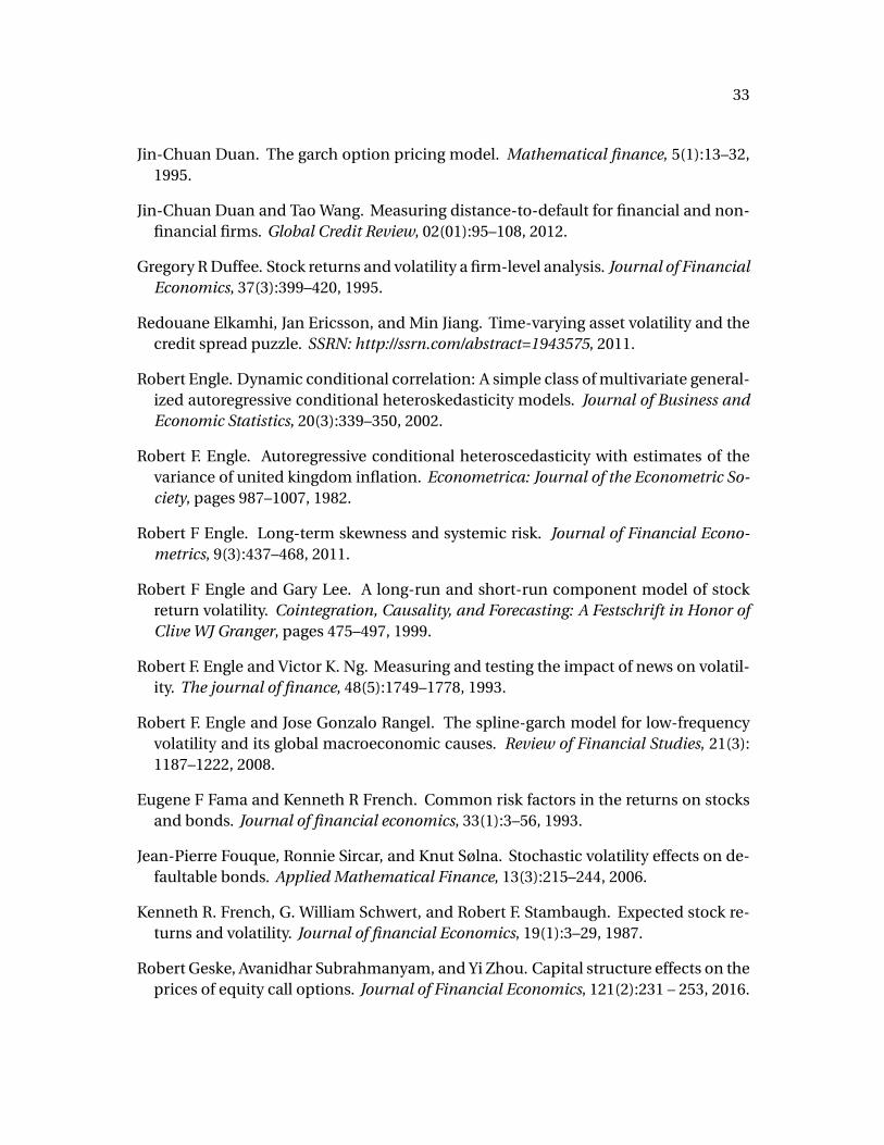
33

Jin-Chuan Duan. The garch option pricing model. Mathematical finance, 5(1):13–32,1995.

Jin-Chuan Duan and Tao Wang. Measuring distance-to-default for financial and non-financial firms. Global Credit Review, 02(01):95–108, 2012.

Gregory R Duffee. Stock returns and volatility a firm-level analysis. Journal of FinancialEconomics, 37(3):399–420, 1995.

Redouane Elkamhi, Jan Ericsson, and Min Jiang. Time-varying asset volatility and thecredit spread puzzle. SSRN: http://ssrn.com/abstract=1943575, 2011.

Robert Engle. Dynamic conditional correlation: A simple class of multivariate general-ized autoregressive conditional heteroskedasticity models. Journal of Business andEconomic Statistics, 20(3):339–350, 2002.

Robert F. Engle. Autoregressive conditional heteroscedasticity with estimates of thevariance of united kingdom inflation. Econometrica: Journal of the Econometric So-ciety, pages 987–1007, 1982.

Robert F Engle. Long-term skewness and systemic risk. Journal of Financial Econo-metrics, 9(3):437–468, 2011.

Robert F Engle and Gary Lee. A long-run and short-run component model of stockreturn volatility. Cointegration, Causality, and Forecasting: A Festschrift in Honor ofClive WJ Granger, pages 475–497, 1999.

Robert F. Engle and Victor K. Ng. Measuring and testing the impact of news on volatil-ity. The journal of finance, 48(5):1749–1778, 1993.

Robert F. Engle and Jose Gonzalo Rangel. The spline-garch model for low-frequencyvolatility and its global macroeconomic causes. Review of Financial Studies, 21(3):1187–1222, 2008.

Eugene F Fama and Kenneth R French. Common risk factors in the returns on stocksand bonds. Journal of financial economics, 33(1):3–56, 1993.

Jean-Pierre Fouque, Ronnie Sircar, and Knut Sølna. Stochastic volatility effects on de-faultable bonds. Applied Mathematical Finance, 13(3):215–244, 2006.

Kenneth R. French, G. William Schwert, and Robert F. Stambaugh. Expected stock re-turns and volatility. Journal of financial Economics, 19(1):3–29, 1987.

Robert Geske, Avanidhar Subrahmanyam, and Yi Zhou. Capital structure effects on theprices of equity call options. Journal of Financial Economics, 121(2):231 – 253, 2016.

34

Lawrence R. Glosten, Ravi Jagannathan, and David E. Runkle. On the relation betweenthe expected value and the volatility of the nominal excess return on stocks. Thejournal of finance, 48(5):1779–1801, 1993.

Dirk Hackbarth, Jianjun Miao, and Erwan Morellec. Capital structure, credit risk, andmacroeconomic conditions. Journal of Financial Economics, 82(3):519–550, 2006.

Jasmina Hasanhodzic and Andrew Lo. Black’s leverage effect is not due to leverage.SSRN: http://ssrn.com/abstract=1762363, 2013.

Steven L. Heston. A closed-form solution for options with stochastic volatility withapplications to bond and currency options. Review of financial studies, 6(2):327–343, 1993.

Hayne E. Leland and Klaus Bjerre Toft. Optimal capital structure, endogenousbankruptcy, and the term structure of credit spreads. The Journal of Finance, 51(3):987–1019, 1996.

Tim McQuade. Stochastic volatility and asset pricing puzzles. Stanford University GSB,Working Paper, 2013.

Robert C Merton. Theory of rational option pricing. The Bell Journal of economics andmanagement science, pages 141–183, 1973.

Robert C. Merton. On the pricing of corporate debt: The risk structure of interest rates.The Journal of Finance, 29(2):449–470, 1974. ISSN 00221082, 15406261.

Robert C. Merton. Option pricing when underlying stock returns are discontinuous.Journal of Financial Economics, 3(1-2):125–144, 1976.

Franco Modigliani and Merton H. Miller. The cost of capital, corporation finance, andthe theory of investment: Reply. The American Economic Review, 49(4):655–669,1959.

Daniel B Nelson. Conditional heteroskedasticity in asset returns: A new approach.Econometrica: Journal of the Econometric Society, pages 347–370, 1991.

Andrew J. Patton. Volatility forecast comparison using imperfect volatility proxies.Journal of Econometrics, 160(1):246–256, 2011.

Stephen M. Schaefer and Ilya A. Strebulaev. Structural models of credit risk are useful:Evidence from hedge ratios on corporate bonds. Journal of Financial Economics, 90(1):1 – 19, 2008.

Emil N. Siriwardane. Concentrated capital losses and the pricing of corporate creditrisk. Harvard Business School Working Paper, 2016.

35

Jeremy Stein and Elias Stein. Stock price distributions with stochastic volatility: Ananalytic approach. Review of Financial Studies, 4:727–752, 1991.

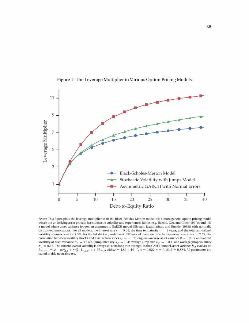
36

Figure 1: The Leverage Multiplier in Various Option Pricing Models

0 5 10 15 20 25 30 35 40Debt-to-Equity Ratio

1

3

5

7

9

11

Leve

rage

Mul

tiplie

r

Black-Scholes-Merton ModelStochastic Volatility with Jumps ModelAsymmetric GARCH with Normal Errors

Notes: This figure plots the leverage multiplier in (i) the Black-Scholes-Merton model; (ii) a more general option pricing modelwhere the underlying asset process has stochastic volatility and experiences jumps (e.g. Bakshi, Cao, and Chen (1997)); and (iii)a model where asset variance follows an asymmetric GARCH model (Glosten, Jagannathan, and Runkle (1993)) with normallydistributed innovations. For all models, the interest rate r = 0.03, the time to maturity ⌧ = 2 years, and the total annualizedvolatility of assets is set to 17.5%. For the Bakshi, Cao, and Chen (1997) model: the speed of volatility mean reversion = 2.77; thecorrelation between volatility shocks and asset return shocks ⇢ = �0.7; long-run average asset variance ✓ = 0.013; annualizedvolatility of asset variance �v = 17.5%; jump intensity �J = 0.4; average jump size µJ = �0.1; and average jump volatility�J = 0.15. The current level of volatility is always set at its long-run average. In the GARCH model, asset variance hA evolves as:hA,t+1 = ! + ↵r2A,t + �r2A,t1rA,t<0 + �hA,t, with ! = 4.86⇥ 10�7,↵ = 0.022, � = 0.18,� = 0.884. All parameters arestated in risk-neutral space.

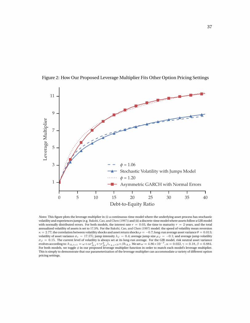
37

Figure 2: How Our Proposed Leverage Multiplier Fits Other Option Pricing Settings

0 5 10 15 20 25 30 35 40Debt-to-Equity Ratio

1

3

5

7

9

11

Leve

rage

Mul

tiplie

r

� = 1.06Stochastic Volatility with Jumps Model� = 1.20Asymmetric GARCH with Normal Errors

Notes: This figure plots the leverage multiplier in (i) a continuous-time model where the underlying asset process has stochasticvolatility and experiences jumps (e.g. Bakshi, Cao, and Chen (1997)) and (ii) a discrete-time model where assets follow a GJR modelwith normally distributed errors. For both models, the interest rate r = 0.03, the time to maturity ⌧ = 2 years, and the totalannualized volatility of assets is set to 17.5%. For the Bakshi, Cao, and Chen (1997) model: the speed of volatility mean reversion = 2.77; the correlation between volatility shocks and asset return shocks⇢ = �0.7; long-run average asset variance ✓ = 0.013;volatility of asset variance �v = 17.5%; jump intensity �J = 0.4; average jump size µJ = �0.1; and average jump volatility�J = 0.15. The current level of volatility is always set at its long-run average. For the GJR model, risk neutral asset varianceevolves according to: hA,t+1 = !+↵r2A,t+�r2A,t1rA,t<0+�hA,t. We set! = 4.86⇥10�7,↵ = 0.022, � = 0.18,� = 0.884.For both models, we toggle � in our proposed leverage multiplier function in order to match each model’s leverage multiplier.This is simply to demonstrate that our parameterization of the leverage multiplier can accommodate a variety of different optionpricing settings.

38

Figure 3: Volatility Risk Pricing and Our Proposed Leverage Multiplier

0 5 10 15 20 25 30 35 401

2

3

4

5

6

7

8

9

10

� = -3.23; �QA = 30.3; Half-Life = 9; � = 0.89

� = -2.77; �QA = 24.7; Half-Life = 6; � = 0.93

� = -1.39; �QA = 17.5; Half-Life = 3; � = 0.99

� = 0.00; �QA = 14.3; Half-Life = 2; � = 1.04

Notes: This figure plots the leverage multiplier in the Heston (1993) model for a variety of parameter values governing the pricingof volatility risk. Under the physical measure, we set = 4.16, ✓ = 0.0204, �v = 0.175, ⇢ = �0.7. These parameterscorrespond to a half-life for asset volatility shocks of 2 months, long-run asset volatility of 14.3%, and a volatility of asset volatilityof 17.5%. We then compute the leverage multiplier for four different values of the price of volatility risk �. In all cases, the interestrate r = 0.03 and the time to maturity ⌧ = 2 years. The current level of physical volatility is always set at its long-run average. Foreach parameter combination, we toggle � in our proposed leverage multiplier function in order to match the leverage multiplierimplied by that parameter combination. The solid lines with markers are the true leverage multiplier under the Heston (1993)model, and the dotted lines show our approximation.

39

Figure 4: How Does the Leverage Multiplier Vary Across Firms and Time?

2000 2002 2004 2006 2008 2010 2012 2014 2016Date

1

2

3

4

5

6

7

8

9

Leve

rage

Mul

tiplie

r

MedianInterquartile Range

Notes: This figure plots the leverage multiplier across firms and through time. We focus on firms for which � 6= 0 because theseare the firms that have a non-constant leverage multiplier. For each firm, we take the estimated daily leverage multiplier andresample it at a weekly frequency by averaging within each week. The solid line is the cross-sectional median within each week,and the shaded bars represent the interquartile range.

40

Figure 5: Volatility and the Leverage Multiplier of the Financial Sector

Panel A (Full Sample):

2000 2002 2004 2006 2008 2010 2012 2014 20160

50

100

150

200

Ann

ualiz

edVo

latil

ity(%

)

0

4

8

12

16

20

24

Leve

rage

Mul

tiplie

r

Fin. Sector Asset Volatility (left)Fin. Sector Equity Volatility (left)Fin. Sector LM (right)

Panel B (Financial Crisis):

May 2007

Sep 2007Jan 2008

May 2008

Sep 2008Jan 2009

May 2009

Sep 2009

0

50

100

150

200

Ann

ualiz

edVo

latil

ity(%

)

0

4

8

12

16

20

Leve

rage

Mul

tiplie

r

Fin. Sector Asset Volatility (left)Fin. Sector Equity Volatility (left)Fin. Sector LM (right)

Notes: This figure plots the equity volatility, asset volatility, and the leverage multiplier of the financial sector. We focus on firms forwhich � 6= 0 because these are the firms that have a non-constant leverage multiplier. For each firm, we take the estimated dailyvolatility or leverage multiplier series and resample it at a weekly frequency by averaging within each week. We then create anaggregate financial sector index at each point in time by taking an asset weighted-average across firms, where assets are proxiedfor by the market value of equity plus the face value of outstanding debt. We smooth the book values of debt using an exponentialaverage (see Section 3.1). The top panel is for the full sample, the bottom panel is from January 2007 through December 2009.

41

Figure 6: The Impact of Capital Injections on One-Month Crash Likelihoods

�100 �95 �90 �85 �80 �75 �70One-Month Ahead Equity Return (%)

0.5

1.0

1.5

2.0

2.5

3.0

3.5

4.0

CD

F(%

)

No Injection (Bankruptcy Probability = 1.32%)With Injection (Bankruptcy Probability = 0.50%)

Notes: This figure plots the simulated cumulative equity return distribution for Bank of America (BAC), with a focus on the lefttail of the distribution. For the simulations, we consider two different models. The first model is the standard Structural GARCHmodel and the second model is the Structural GARCH model where BAC has received an equity injection. All of the models aresimulated using data as of 10/27/2008. The smoothed debt amount on this date was $1562.2 bn and the market value of equitywas $93.6 bn. The amount of the injection corresponds to what BAC received from the U.S. government on 10/28/2008. For bothmodels, we use the same set of standard normal shocks and simulate 10 million paths out to a horizon of one-month.

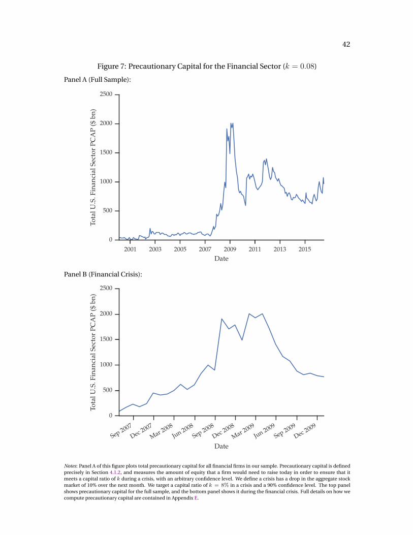
42

Figure 7: Precautionary Capital for the Financial Sector (k = 0.08)

Panel A (Full Sample):

2001 2003 2005 2007 2009 2011 2013 2015Date

0

500

1000

1500

2000

2500To

talU

.S.F

inan

cial

Sect

orPC

AP

($bn

)

Panel B (Financial Crisis):

Sep 2007

Dec 2007

Mar 2008

Jun 2008

Sep 2008

Dec 2008

Mar 2009

Jun 2009

Sep 2009

Dec 2009

Date

0

500

1000

1500

2000

2500

Tota

lU.S

.Fin

anci

alSe

ctor

PCA

P($

bn)

Notes: Panel A of this figure plots total precautionary capital for all financial firms in our sample. Precautionary capital is definedprecisely in Section 4.1.2, and measures the amount of equity that a firm would need to raise today in order to ensure that itmeets a capital ratio of k during a crisis, with an arbitrary confidence level. We define a crisis has a drop in the aggregate stockmarket of 10% over the next month. We target a capital ratio of k = 8% in a crisis and a 90% confidence level. The top panelshows precautionary capital for the full sample, and the bottom panel shows it during the financial crisis. Full details on how wecompute precautionary capital are contained in Appendix E.

43

Figure 8: Volatility Asymmetry Measured with Simple Correlations

Panel A (Equity Versus Assets Returns):

�0.25 �0.20 �0.15 �0.10 �0.05 0.00 0.05 0.10 0.15�(|rt+1|, rt) for Equity

�0.25

�0.20

�0.15

�0.10

�0.05

0.00

0.05

0.10

0.15�(

|r t+

1|,r t

)fo

rAss

ets

45-Degree Line

Panel B (Equity Versus Idiosyncratic Asset Returns):

�0.25 �0.20 �0.15 �0.10 �0.05 0.00 0.05 0.10 0.15�(|rt+1|, rt) for Equity

�0.25

�0.20

�0.15

�0.10

�0.05

0.00

0.05

0.10

0.15

�(|r t

+1|,

r t)

forI

dios

yncr

atic

Ass

etR

etur

ns

45-Degree Line

Notes: This figure plots a measure of volatility asymmetry in equity returns against the same measure in: (i) asset returns (PanelA) and (ii) idiosyncratic asset returns (Panel B). Volatility asymmetry is measured as the correlation between the absolute value ofreturns at time t and returns at time t � 1. Asset returns are computed using the leverage multiplier from the Structural GARCHmodel, and are simply equity returns divided by the lagged leverage multiplier. Idiosyncratic asset returns are defined as theresiduals from a regression of asset returns on the CRSP value-weighted index.

44

Figure 9: Volatility Asymmetry Measured from the GJR Model

Panel A (Equity Versus Assets Returns):

�0.1 0.0 0.1 0.2 0.3 0.4� for Equity

�0.1

0.0

0.1

0.2

0.3

0.4�

forA

sset

s

45-Degree Line

Panel B (Equity Versus Idiosyncratic Asset Returns):

�0.1 0.0 0.1 0.2 0.3 0.4� for Equity

�0.1

0.0

0.1

0.2

0.3

0.4

�fo

rIdi

osyn

crat

icA

sset

Ret

urns

45-Degree Line

Notes: This figure plots a measure of volatility asymmetry in equity returns against the same measure in: (i) asset returns (PanelA) and (ii) idiosyncratic asset returns (Panel B). Volatility asymmetry is defined as the parameter in the Glosten, Jagannathan, andRunkle (1993) model that measures the response of variance to negative return news (�). Asset returns are computed using theleverage multiplier from the Structural GARCH model, and are simply equity returns divided by the lagged leverage multiplier.Idiosyncratic asset returns are defined as the residuals from a regression of asset returns on the CRSP value-weighted index.

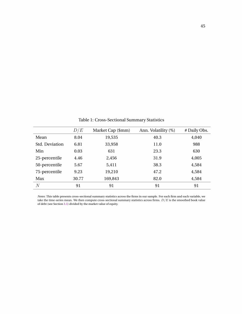
45

Table 1: Cross-Sectional Summary Statistics

D/E Market Cap ($mm) Ann. Volatility (%) # Daily Obs.

Mean 8.04 19,535 40.3 4,040

Std. Deviation 6.81 33,958 11.0 988

Min 0.03 631 23.3 630

25-percentile 4.46 2,456 31.9 4,005

50-percentile 5.67 5,411 38.3 4,584

75-percentile 9.23 19,210 47.2 4,584

Max 30.77 169,843 82.0 4,584

N 91 91 91 91

Notes: This table presents cross-sectional summary statistics across the firms in our sample. For each firm and each variable, wetake the time-series mean. We then compute cross-sectional summary statistics across firms. D/E is the smoothed book valueof debt (see Section 3.1) divided by the market value of equity.

46

Table 2: Estimated Parameters and t-statistics of the Structural GARCH Model

! ↵ � � �

Mean:Point Estimate 2.74e-6 0.047 0.074 0.902 0.738

t-statistic 1.23 2.76 2.83 72.07 3.42

25-percentile:Point Estimate 2.66e-7 0.023 0.046 0.884 0.054

t-statistic 0.80 1.98 1.96 48.01 0.07

50-percentile:Point Estimate 7.30e-7 0.041 0.071 0.914 0.680

t-statistic 1.12 2.91 3.01 71.24 2.36

75-percentile:Point Estimate 4.47e-6 0.063 0.094 0.931 1.003

t-statistic 1.57 3.57 3.84 91.76 4.64

% of Firms with |t| � 1.64 22.0 81.3 82.4 100 60.4

Notes: This table presents summary statistics across firms of the point estimates from the Structural GARCH model. The fullspecification of the Structural GARCH model can be found in Equation (5). The total number of firms in our sample is 91, and afull list can be found in INSERT. For each firm, we estimate the model using daily data. Full details of the estimation procedurecan be found in Section 3. All reported t-statistics are QMLE robust (Bollerslev-Wooldridge).

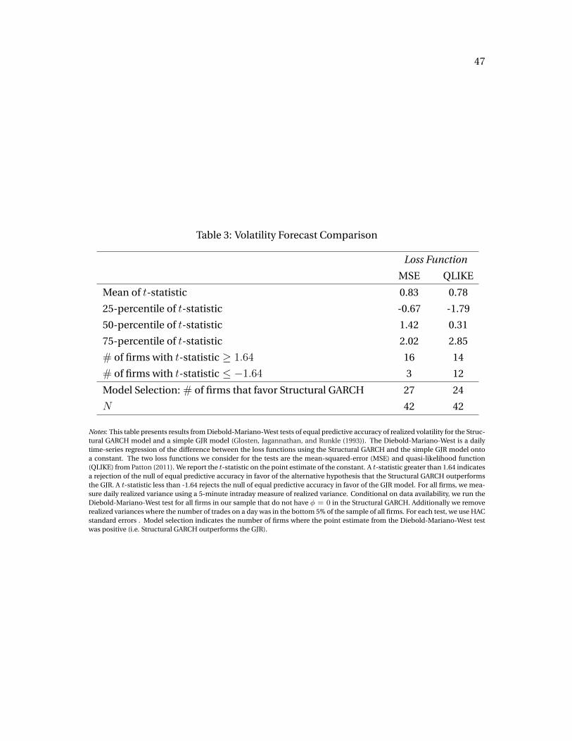
47

Table 3: Volatility Forecast Comparison

Loss Function

MSE QLIKE

Mean of t-statistic 0.83 0.78

25-percentile of t-statistic -0.67 -1.79

50-percentile of t-statistic 1.42 0.31

75-percentile of t-statistic 2.02 2.85

# of firms with t-statistic � 1.64 16 14

# of firms with t-statistic �1.64 3 12

Model Selection: # of firms that favor Structural GARCH 27 24

N 42 42

Notes: This table presents results from Diebold-Mariano-West tests of equal predictive accuracy of realized volatility for the Struc-tural GARCH model and a simple GJR model (Glosten, Jagannathan, and Runkle (1993)). The Diebold-Mariano-West is a dailytime-series regression of the difference between the loss functions using the Structural GARCH and the simple GJR model ontoa constant. The two loss functions we consider for the tests are the mean-squared-error (MSE) and quasi-likelihood function(QLIKE) from Patton (2011). We report the t-statistic on the point estimate of the constant. A t-statistic greater than 1.64 indicatesa rejection of the null of equal predictive accuracy in favor of the alternative hypothesis that the Structural GARCH outperformsthe GJR. A t-statistic less than -1.64 rejects the null of equal predictive accuracy in favor of the GJR model. For all firms, we mea-sure daily realized variance using a 5-minute intraday measure of realized variance. Conditional on data availability, we run theDiebold-Mariano-West test for all firms in our sample that do not have � = 0 in the Structural GARCH. Additionally we removerealized variances where the number of trades on a day was in the bottom 5% of the sample of all firms. For each test, we use HACstandard errors . Model selection indicates the number of firms where the point estimate from the Diebold-Mariano-West testwas positive (i.e. Structural GARCH outperforms the GJR).

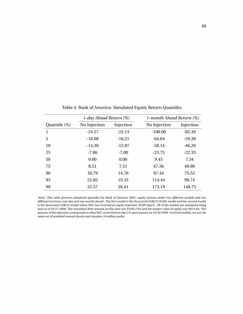
48

Table 4: Bank of America: Simulated Equity Return Quantiles

1-day Ahead Return (%) 1-month Ahead Return (%)

Quantile (%) No Injection Injection No Injection Injection

1 -24.57 -22.13 -100.00 -82.49

5 -18.08 -16.21 -64.64 -59.38

10 -14.39 -12.87 -50.14 -46.26

25 -7.86 -7.00 -23.75 -22.33

50 0.00 0.00 9.45 7.34

75 8.51 7.51 47.56 40.88

90 16.79 14.76 87.44 75.52

95 22.05 19.33 114.44 98.74

99 32.57 28.41 173.19 148.75

Notes: This table presents simulated quantiles for Bank of America (BAC) equity returns under two different models and twodifferent horizons (one day and one month ahead). The first model is the Structural GARCH (SGJR) model and the second modelis the Structural GARCH model where BAC has received an equity injection (SGJR-Inject). All of the models are simulated usingdata as of 10/27/2008. The smoothed debt amount on this date was $1562.2 bn and the market value of equity was $93.6 bn. Theamount of the injection corresponds to what BAC received from the U.S. government on 10/28/2008. For both models, we use thesame set of standard normal shocks and simulate 10 million paths.

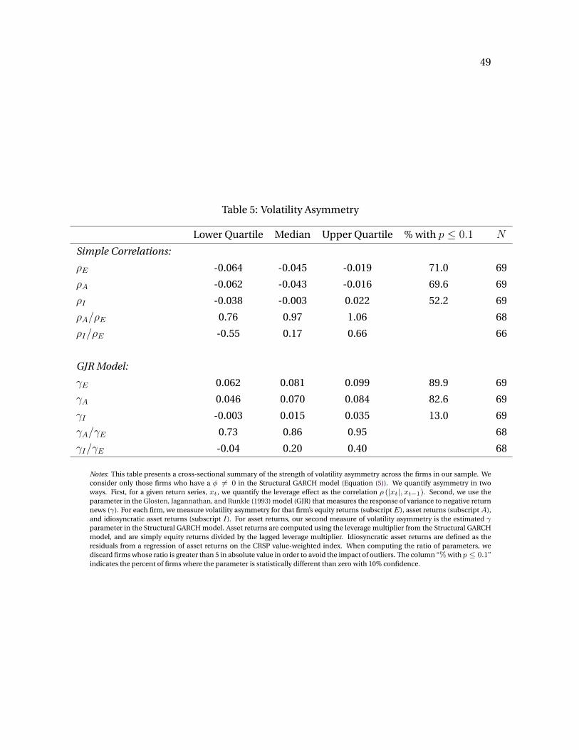
49

Table 5: Volatility Asymmetry

Lower Quartile Median Upper Quartile % with p 0.1 N

Simple Correlations:

⇢E -0.064 -0.045 -0.019 71.0 69

⇢A -0.062 -0.043 -0.016 69.6 69

⇢I -0.038 -0.003 0.022 52.2 69

⇢A/⇢E 0.76 0.97 1.06 68

⇢I/⇢E -0.55 0.17 0.66 66

GJR Model:

�E 0.062 0.081 0.099 89.9 69

�A 0.046 0.070 0.084 82.6 69

�I -0.003 0.015 0.035 13.0 69

�A/�E 0.73 0.86 0.95 68

�I/�E -0.04 0.20 0.40 68

Notes: This table presents a cross-sectional summary of the strength of volatility asymmetry across the firms in our sample. Weconsider only those firms who have a � 6= 0 in the Structural GARCH model (Equation (5)). We quantify asymmetry in twoways. First, for a given return series, xt, we quantify the leverage effect as the correlation ⇢ (|xt|, xt�1). Second, we use theparameter in the Glosten, Jagannathan, and Runkle (1993) model (GJR) that measures the response of variance to negative returnnews (�). For each firm, we measure volatility asymmetry for that firm’s equity returns (subscript E), asset returns (subscript A),and idiosyncratic asset returns (subscript I). For asset returns, our second measure of volatility asymmetry is the estimated �parameter in the Structural GARCH model. Asset returns are computed using the leverage multiplier from the Structural GARCHmodel, and are simply equity returns divided by the lagged leverage multiplier. Idiosyncratic asset returns are defined as theresiduals from a regression of asset returns on the CRSP value-weighted index. When computing the ratio of parameters, wediscard firms whose ratio is greater than 5 in absolute value in order to avoid the impact of outliers. The column “% with p 0.1”indicates the percent of firms where the parameter is statistically different than zero with 10% confidence.

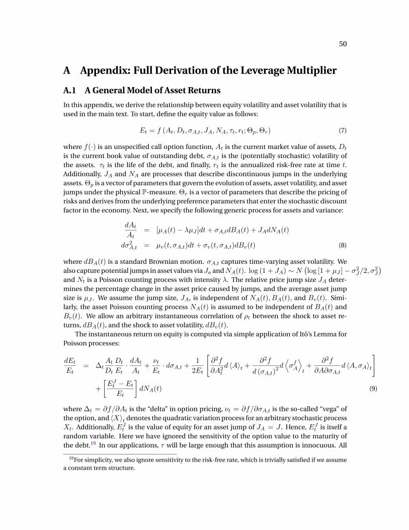
50

A Appendix: Full Derivation of the Leverage Multiplier

A.1 A General Model of Asset Returns

In this appendix, we derive the relationship between equity volatility and asset volatility that isused in the main text. To start, define the equity value as follows:

Et = f (At, Dt,�A,t, JA, NA, ⌧t, rt; ⇥p,⇥r) (7)

where f(·) is an unspecified call option function, At is the current market value of assets, Dt

is the current book value of outstanding debt, �A,t is the (potentially stochastic) volatility ofthe assets. ⌧t is the life of the debt, and finally, rt is the annualized risk-free rate at time t.Additionally, JA and NA are processes that describe discontinuous jumps in the underlyingassets. ⇥p is a vector of parameters that govern the evolution of assets, asset volatility, and assetjumps under the physical P-measure. ⇥r is a vector of parameters that describe the pricing ofrisks and derives from the underlying preference parameters that enter the stochastic discountfactor in the economy. Next, we specify the following generic process for assets and variance:

dAt

At= [µA(t) � �µJ ]dt + �A,tdBA(t) + JAdNA(t)

d�

2A,t = µv(t,�A,t)dt + �v(t,�A,t)dBv(t) (8)

where dBA(t) is a standard Brownian motion. �A,t captures time-varying asset volatility. Wealso capture potential jumps in asset values viaJa andNA(t). log (1 + JA) ⇠ N

�log [1 + µJ ] � �

2J/2,�

2J

�

and Nt is a Poisson counting process with intensity �. The relative price jump size JA deter-mines the percentage change in the asset price caused by jumps, and the average asset jumpsize is µJ . We assume the jump size, JA, is independent of NA(t), BA(t), and Bv(t). Simi-larly, the asset Poisson counting process NA(t) is assumed to be independent of BA(t) andBv(t). We allow an arbitrary instantaneous correlation of ⇢t between the shock to asset re-turns, dBA(t), and the shock to asset volatility, dBv(t).

The instantaneous return on equity is computed via simple application of Ito’s Lemma forPoisson processes:

dEt

Et= �t

At

Dt

Dt

Et· dAt

At+

⌫t

Et· d�A,t +

1

2Et

"@

2f

@A

2t

d hAit +

@

2f

d (�A,t)2d

D�

fA

E

t+

@

2f

@A@�A,td hA,�Ait

#

+

E

Jt � Et

Et

�dNA(t) (9)

where �t = @f/@At is the “delta” in option pricing, ⌫t = @f/@�A,t is the so-called “vega” ofthe option, and hXit denotes the quadratic variation process for an arbitrary stochastic processXt. Additionally, EJ

t is the value of equity for an asset jump of JA = J . Hence, EJt is itself a

random variable. Here we have ignored the sensitivity of the option value to the maturity ofthe debt.19 In our applications, ⌧ will be large enough that this assumption is innocuous. All

19For simplicity, we also ignore sensitivity to the risk-free rate, which is trivially satisfied if we assumea constant term structure.

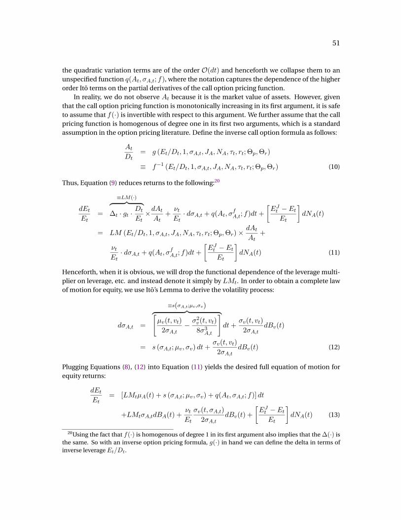
51

the quadratic variation terms are of the order O(dt) and henceforth we collapse them to anunspecified function q(At,�A,t; f), where the notation captures the dependence of the higherorder Ito terms on the partial derivatives of the call option pricing function.

In reality, we do not observe At because it is the market value of assets. However, giventhat the call option pricing function is monotonically increasing in its first argument, it is safeto assume that f(·) is invertible with respect to this argument. We further assume that the callpricing function is homogenous of degree one in its first two arguments, which is a standardassumption in the option pricing literature. Define the inverse call option formula as follows:

At

Dt= g (Et/Dt, 1,�A,t, JA, NA, ⌧t, rt; ⇥p,⇥r)

⌘ f

�1(Et/Dt, 1,�A,t, JA, NA, ⌧t, rt; ⇥p,⇥r) (10)

Thus, Equation (9) reduces returns to the following:20

dEt

Et=

⌘LM(·)z }| {�t · gt · Dt

Et⇥dAt

At+

⌫t

Et· d�A,t + q(At,�

fA,t; f)dt +

E

Jt � Et

Et

�dNA(t)

= LM (Et/Dt, 1,�A,t, JA, NA, ⌧t, rt; ⇥p,⇥r) ⇥ dAt

At+

⌫t

Et· d�A,t + q(At,�

fA,t; f)dt +

E

Jt � Et

Et

�dNA(t) (11)

Henceforth, when it is obvious, we will drop the functional dependence of the leverage multi-plier on leverage, etc. and instead denote it simply by LMt. In order to obtain a complete lawof motion for equity, we use Ito’s Lemma to derive the volatility process:

d�A,t =

⌘s(

�A,t;µv ,�v)

z }| {"µv(t, vt)

2�A,t� �

2v(t, vt)

8�

3A,t

#dt +

�v(t, vt)

2�A,tdBv(t)

= s (�A,t;µv,�v) dt +

�v(t, vt)

2�A,tdBv(t) (12)

Plugging Equations (8), (12) into Equation (11) yields the desired full equation of motion forequity returns:

dEt

Et= [LMtµA(t) + s (�A,t;µv,�v) + q(At,�A,t; f)] dt

+LMt�A,tdBA(t) +

⌫t

Et

�v(t,�A,t)

2�A,tdBv(t) +

E

Jt � Et

Et

�dNA(t) (13)

20Using the fact that f(·) is homogenous of degree 1 in its first argument also implies that the �(·) isthe same. So with an inverse option pricing formula, g(·) in hand we can define the delta in terms ofinverse leverage Et/Dt.

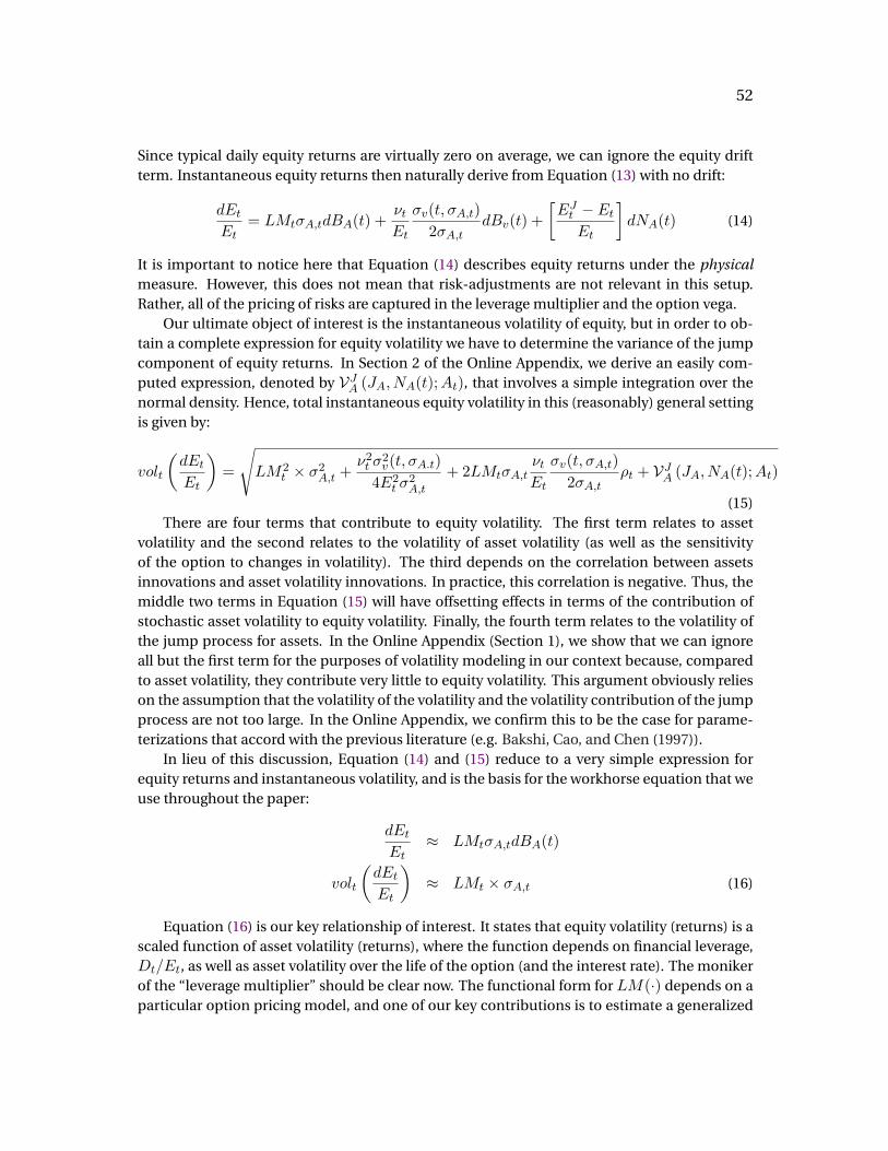
52

Since typical daily equity returns are virtually zero on average, we can ignore the equity driftterm. Instantaneous equity returns then naturally derive from Equation (13) with no drift:

dEt

Et= LMt�A,tdBA(t) +

⌫t

Et

�v(t,�A,t)

2�A,tdBv(t) +

E

Jt � Et

Et

�dNA(t) (14)

It is important to notice here that Equation (14) describes equity returns under the physicalmeasure. However, this does not mean that risk-adjustments are not relevant in this setup.Rather, all of the pricing of risks are captured in the leverage multiplier and the option vega.

Our ultimate object of interest is the instantaneous volatility of equity, but in order to ob-tain a complete expression for equity volatility we have to determine the variance of the jumpcomponent of equity returns. In Section 2 of the Online Appendix, we derive an easily com-puted expression, denoted by VJ

A (JA, NA(t);At), that involves a simple integration over thenormal density. Hence, total instantaneous equity volatility in this (reasonably) general settingis given by:

volt

✓dEt

Et

◆=

s

LM

2t ⇥ �

2A,t +

⌫

2t �

2v(t,�A.t)

4E

2t �

2A,t

+ 2LMt�A,t⌫t

Et

�v(t,�A,t)

2�A,t⇢t + VJ

A (JA, NA(t);At)

(15)There are four terms that contribute to equity volatility. The first term relates to asset

volatility and the second relates to the volatility of asset volatility (as well as the sensitivityof the option to changes in volatility). The third depends on the correlation between assetsinnovations and asset volatility innovations. In practice, this correlation is negative. Thus, themiddle two terms in Equation (15) will have offsetting effects in terms of the contribution ofstochastic asset volatility to equity volatility. Finally, the fourth term relates to the volatility ofthe jump process for assets. In the Online Appendix (Section 1), we show that we can ignoreall but the first term for the purposes of volatility modeling in our context because, comparedto asset volatility, they contribute very little to equity volatility. This argument obviously relieson the assumption that the volatility of the volatility and the volatility contribution of the jumpprocess are not too large. In the Online Appendix, we confirm this to be the case for parame-terizations that accord with the previous literature (e.g. Bakshi, Cao, and Chen (1997)).

In lieu of this discussion, Equation (14) and (15) reduce to a very simple expression forequity returns and instantaneous volatility, and is the basis for the workhorse equation that weuse throughout the paper:

dEt

Et⇡ LMt�A,tdBA(t)

volt

✓dEt

Et

◆⇡ LMt ⇥ �A,t (16)

Equation (16) is our key relationship of interest. It states that equity volatility (returns) is ascaled function of asset volatility (returns), where the function depends on financial leverage,Dt/Et, as well as asset volatility over the life of the option (and the interest rate). The monikerof the “leverage multiplier” should be clear now. The functional form for LM(·) depends on aparticular option pricing model, and one of our key contributions is to estimate a generalized

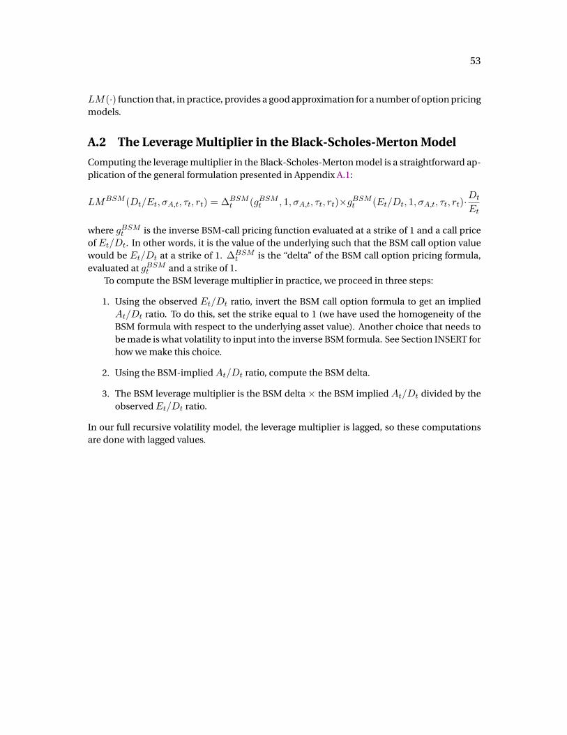
53

LM(·) function that, in practice, provides a good approximation for a number of option pricingmodels.

A.2 The Leverage Multiplier in the Black-Scholes-Merton Model

Computing the leverage multiplier in the Black-Scholes-Merton model is a straightforward ap-plication of the general formulation presented in Appendix A.1:

LM

BSM(Dt/Et,�A,t, ⌧t, rt) = �

BSMt (g

BSMt , 1,�A,t, ⌧t, rt)⇥g

BSMt (Et/Dt, 1,�A,t, ⌧t, rt)·Dt

Et

where g

BSMt is the inverse BSM-call pricing function evaluated at a strike of 1 and a call price

of Et/Dt. In other words, it is the value of the underlying such that the BSM call option valuewould be Et/Dt at a strike of 1. �

BSMt is the “delta” of the BSM call option pricing formula,

evaluated at gBSMt and a strike of 1.

To compute the BSM leverage multiplier in practice, we proceed in three steps:

1. Using the observed Et/Dt ratio, invert the BSM call option formula to get an impliedAt/Dt ratio. To do this, set the strike equal to 1 (we have used the homogeneity of theBSM formula with respect to the underlying asset value). Another choice that needs tobe made is what volatility to input into the inverse BSM formula. See Section INSERT forhow we make this choice.

2. Using the BSM-implied At/Dt ratio, compute the BSM delta.

3. The BSM leverage multiplier is the BSM delta ⇥ the BSM implied At/Dt divided by theobserved Et/Dt ratio.

In our full recursive volatility model, the leverage multiplier is lagged, so these computationsare done with lagged values.

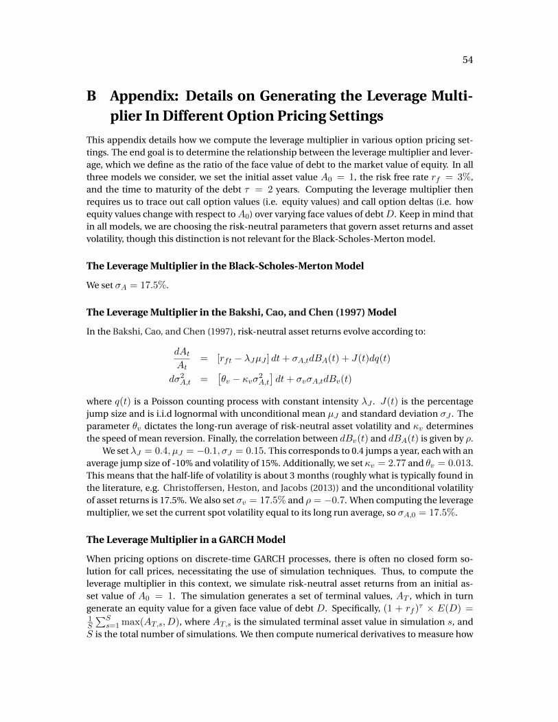
54

B Appendix: Details on Generating the Leverage Multi-plier In Different Option Pricing Settings

This appendix details how we compute the leverage multiplier in various option pricing set-tings. The end goal is to determine the relationship between the leverage multiplier and lever-age, which we define as the ratio of the face value of debt to the market value of equity. In allthree models we consider, we set the initial asset value A0 = 1, the risk free rate rf = 3%,and the time to maturity of the debt ⌧ = 2 years. Computing the leverage multiplier thenrequires us to trace out call option values (i.e. equity values) and call option deltas (i.e. howequity values change with respect to A0) over varying face values of debt D. Keep in mind thatin all models, we are choosing the risk-neutral parameters that govern asset returns and assetvolatility, though this distinction is not relevant for the Black-Scholes-Merton model.

The Leverage Multiplier in the Black-Scholes-Merton Model

We set �A = 17.5%.

The Leverage Multiplier in the Bakshi, Cao, and Chen (1997) Model

In the Bakshi, Cao, and Chen (1997), risk-neutral asset returns evolve according to:

dAt

At= [rft � �JµJ ] dt + �A,tdBA(t) + J(t)dq(t)

d�

2A,t =

⇥✓v � v�

2A,t

⇤dt + �v�A,tdBv(t)

where q(t) is a Poisson counting process with constant intensity �J . J(t) is the percentagejump size and is i.i.d lognormal with unconditional mean µJ and standard deviation �J . Theparameter ✓v dictates the long-run average of risk-neutral asset volatility and v determinesthe speed of mean reversion. Finally, the correlation between dBv(t) and dBA(t) is given by ⇢.

We set �J = 0.4, µJ = �0.1,�J = 0.15. This corresponds to 0.4 jumps a year, each with anaverage jump size of -10% and volatility of 15%. Additionally, we set v = 2.77 and ✓v = 0.013.This means that the half-life of volatility is about 3 months (roughly what is typically found inthe literature, e.g. Christoffersen, Heston, and Jacobs (2013)) and the unconditional volatilityof asset returns is 17.5%. We also set �v = 17.5% and ⇢ = �0.7. When computing the leveragemultiplier, we set the current spot volatility equal to its long run average, so �A,0 = 17.5%.

The Leverage Multiplier in a GARCH Model

When pricing options on discrete-time GARCH processes, there is often no closed form so-lution for call prices, necessitating the use of simulation techniques. Thus, to compute theleverage multiplier in this context, we simulate risk-neutral asset returns from an initial as-set value of A0 = 1. The simulation generates a set of terminal values, AT , which in turngenerate an equity value for a given face value of debt D. Specifically, (1 + rf )

⌧ ⇥ E(D) =

1S

PSs=1 max(AT,s, D), where AT,s is the simulated terminal asset value in simulation s, and

S is the total number of simulations. We then compute numerical derivatives to measure how

55

the equity value changes with respect to A0. Finally, we obtain the leverage multiplier overvarying D/E values.

The asymmetric GARCH model that we use for risk-neutral asset returns is as follows:

rA,t =

phA,t"A,t

hA,t = ! + ↵r

2A,t�1 + �r

2A,t�11rA,t�1<0 + �hA,t�1

where 1x<a is an indicator variable that equals 1 if x < a and 0 otherwise. "A,t is a standardnormal shock. The parameter � captures volatility asymmetry and a positive � effectively cap-tures the negative correlation between asset returns and volatility. We parameterize the risk-neutral GARCH process as: ! = 4.86e � 7, ↵ = 0.022, � = 0.18, � = 0.884. These parametersimply that the long-run risk-neutral volatility of assets is also 17.5%. We choose a large � toemphasize the impact that volatility asymmetry has on the leverage multiplier.

56

C Appendix: Cumulative Asset Volatility Forecast in theStructural GARCH Model

Recall that asset variance in the Structural GARCH model evolves according to:

hA,t+1 = ! + ↵r

2A,t�1 + �↵r

2A,t�11rA,t�1<0 + �hA,t

We want to know the cumulative volatility forecast for assets over the period t + 1, ..., t + h,where h is the number of days until maturity. In the notation of the model, this is simply ⌧t ⇥365. Some tedious algebra implies the following closed form for this forecast:

hX

i=1

hA,t+i =

!

1 � ✓

h � !

1 � ✓

· 1 � ✓

h

1 � ✓

+

1 � ✓

h

1 � ✓

⇥ hA,t+1

where ✓ = ↵ + �/2 + �. Note that hA,t+1 is in the information set at time t.

D Appendix: Measuring Realized Variance

Depending on data availability, we compute a daily measure of realized variance using 5-minuteintraday returns. This means we just sum up the squared 5-minute intraday returns withineach day. We generally follow the steps suggested by Andersen, Bollerslev, Diebold, and Labys(2003) in cleaning the intraday TAQ data, though the cleaning choices are not as big of an issuesgiven that we are using 5-min returns and not tick-by-tick data. The main steps in this processare as follows: (i) if several trades have the same time stamp, we use the median price; (ii) weonly use trades from one exchange for each asset; (iii) we filter out trades that are flagged inany way by TAQ; (iv) 5 minute returns that are larger than 10% in absolute value are set to zero,though these are very rare; (v) if the realized variance for a given 5-minute subsample is largerthan 3 times the median RV of all the subsamples in a given day, that subsample is ignored.

We were able to compute a 5-minute realized variance series for 42 out of the 91 firms inour sample. For each firm and date pair, we count the number of trades that occurred for thatfirm. We further discard firm-date observations where the number of trades is in the bottom5% of our entire sample. This mainly affects firms at the early part of the sample given thathigher frequency trading was still in its early stages.

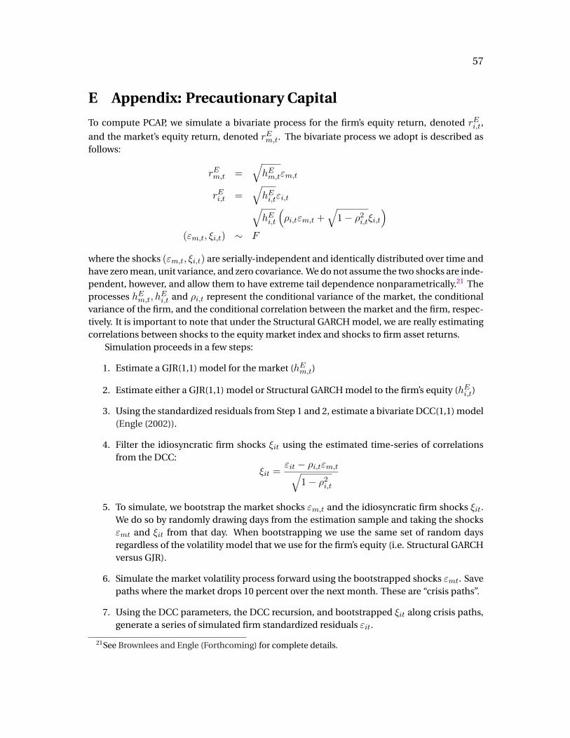
57

E Appendix: Precautionary Capital

To compute PCAP, we simulate a bivariate process for the firm’s equity return, denoted r

Ei,t,

and the market’s equity return, denoted r

Em,t. The bivariate process we adopt is described as

follows:

r

Em,t =

qh

Em,t"m,t

r

Ei,t =

qh

Ei,t"i,t

qh

Ei,t

⇣⇢i,t"m,t +

q1 � ⇢

2i,t⇠i,t

⌘

("m,t, ⇠i,t) ⇠ F

where the shocks ("m,t, ⇠i,t) are serially-independent and identically distributed over time andhave zero mean, unit variance, and zero covariance. We do not assume the two shocks are inde-pendent, however, and allow them to have extreme tail dependence nonparametrically.21 Theprocesses hEm,t, h

Ei,t and ⇢i,t represent the conditional variance of the market, the conditional

variance of the firm, and the conditional correlation between the market and the firm, respec-tively. It is important to note that under the Structural GARCH model, we are really estimatingcorrelations between shocks to the equity market index and shocks to firm asset returns.

Simulation proceeds in a few steps:

1. Estimate a GJR(1,1) model for the market (hEm,t)

2. Estimate either a GJR(1,1) model or Structural GARCH model to the firm’s equity (hEi,t)

3. Using the standardized residuals from Step 1 and 2, estimate a bivariate DCC(1,1) model(Engle (2002)).

4. Filter the idiosyncratic firm shocks ⇠it using the estimated time-series of correlationsfrom the DCC:

⇠it =

"it � ⇢i,t"m,tq1 � ⇢

2i,t

5. To simulate, we bootstrap the market shocks "m,t and the idiosyncratic firm shocks ⇠it.We do so by randomly drawing days from the estimation sample and taking the shocks"mt and ⇠it from that day. When bootstrapping we use the same set of random daysregardless of the volatility model that we use for the firm’s equity (i.e. Structural GARCHversus GJR).

6. Simulate the market volatility process forward using the bootstrapped shocks "mt. Savepaths where the market drops 10 percent over the next month. These are “crisis paths”.

7. Using the DCC parameters, the DCC recursion, and bootstrapped ⇠it along crisis paths,generate a series of simulated firm standardized residuals "it.

21See Brownlees and Engle (Forthcoming) for complete details.

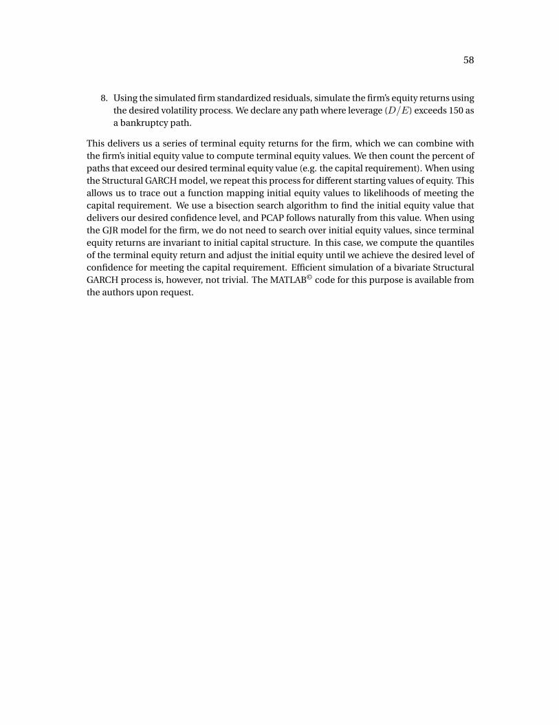
58

8. Using the simulated firm standardized residuals, simulate the firm’s equity returns usingthe desired volatility process. We declare any path where leverage (D/E) exceeds 150 asa bankruptcy path.

This delivers us a series of terminal equity returns for the firm, which we can combine withthe firm’s initial equity value to compute terminal equity values. We then count the percent ofpaths that exceed our desired terminal equity value (e.g. the capital requirement). When usingthe Structural GARCH model, we repeat this process for different starting values of equity. Thisallows us to trace out a function mapping initial equity values to likelihoods of meeting thecapital requirement. We use a bisection search algorithm to find the initial equity value thatdelivers our desired confidence level, and PCAP follows naturally from this value. When usingthe GJR model for the firm, we do not need to search over initial equity values, since terminalequity returns are invariant to initial capital structure. In this case, we compute the quantilesof the terminal equity return and adjust the initial equity until we achieve the desired level ofconfidence for meeting the capital requirement. Efficient simulation of a bivariate StructuralGARCH process is, however, not trivial. The MATLAB© code for this purpose is available fromthe authors upon request.

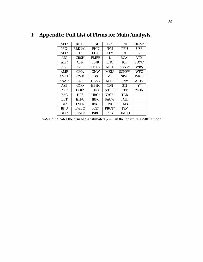
59

F Appendix: Full List of Firms for Main Analysis

AEL* BOKF FGL IVZ PNC UNM*AFG* BRK (A)* FHN JPM PRU USBAFL* C FITB KEY RF VAIG CBSH FMER L RGA* VLYAIZ* CFR FNB LNC RJF VOYA*ALL CIT FNFG MET SBNY* WBSAMP CMA GNW MKL* SCHW* WFC

AMTD CME GS MS SIVB WRB*ANAT* CNA HBAN MTB SNV WTFC

ASB CNO HBHC NNI STI Y*AXP COF* HIG NTRS* STT ZIONBAC DFS HRG* NYCB* TCBBBT ETFC IBKC PACW TCBIBK* EVER IBKR PB TMKBKU EWBC ICE* PBCT* TRVBLK* FCNCA ISBC PFG UMPQ

Notes: * indicates the firm had a estimated � = 0 in the Structural GARCH model