Stochastic Partial Differential Equations withMultiplicative NoiseNumerical simulations of strong and weak approximation errors

Thesis for the degree of Master of Science

Andreas Petersson

Mathematical SciencesChalmers University of TechnologyUniversity of GothenburgGothenburg, Sweden, 15 May 2015

Abstract

A finite element Galerkin spatial discretization together with a backward Eulerscheme is implemented to simulate strong error rates of the homogeneous stochasticheat equation with multiplicative trace class noise in one dimension. For the noise,two different operators displaying different degrees of regularity are considered, oneof which is of Nemytskii type. The discretization scheme is extended to include dis-cretization of the covariance operator of the Q-Wiener process driving the equation.The results agree with the theory. Furthermore, for exploratory reasons, weak errorrates are also simulated using the classical Monte Carlo method and the multilevelMonte Carlo method.

Acknowledgements

First of all I would like to thank my supervisor Associate Professor Annika Langfor a tremendous amount of support and advice during the entirety of this project,as well as for getting me interested in this fascinating field from the get-go. Ithas been an exciting and entertaining, if at times challenging, experience. Thankyou also to all who contributed to the course material of Numerical Analysis ofStochastic Partial Differential Equations at ETH Zurich, it was very helpful forgetting me started. I would also like to thank Professor Stig Larsson for grantingme access to the computational resources at Chalmers Centre for ComputationalScience and Engineering (C3SE) provided by the Swedish National Infrastructurefor Computing (SNIC). Thank you also to Johan Alvbring at C3SE for installingMATLAB Distributed Computing Server on the C3SE resources and providingsupport and documentation to make my simulations run on them. Finally I wouldlike to thank my partner Andrea and the rest of my family for their moral supportand admirable amount of patience with me during the work.

i

ii

Contents

1 Introduction 11.1 Outline of the thesis . . . . . . . . . . . . . . . . . . . . . . . . . . . . . 31.2 On notation . . . . . . . . . . . . . . . . . . . . . . . . . . . . . . . . . . 3

2 Stochastic calculus in Hilbert spaces 42.1 Hilbert-Schmidt spaces and trace class operators . . . . . . . . . . . . . 42.2 Semigroups and fractional powers of operators . . . . . . . . . . . . . . . 62.3 Random variables . . . . . . . . . . . . . . . . . . . . . . . . . . . . . . . 82.4 Q-Wiener Processes . . . . . . . . . . . . . . . . . . . . . . . . . . . . . 102.5 Stochastic integrals . . . . . . . . . . . . . . . . . . . . . . . . . . . . . . 11

3 Semilinear stochastic partial differential equations 133.1 Setting and assumptions . . . . . . . . . . . . . . . . . . . . . . . . . . . 133.2 Strong and mild solutions . . . . . . . . . . . . . . . . . . . . . . . . . . 143.3 Existence and uniqueness of the mild solution . . . . . . . . . . . . . . . 15

4 Discretization methods for SPDE 164.1 Galerkin finite element methods . . . . . . . . . . . . . . . . . . . . . . . 164.2 The implicit Euler scheme . . . . . . . . . . . . . . . . . . . . . . . . . . 174.3 A fully discrete strong approximation of the SPDE . . . . . . . . . . . . 184.4 Noise approximation . . . . . . . . . . . . . . . . . . . . . . . . . . . . . 18

5 Monte Carlo methods 245.1 Strong and weak errors . . . . . . . . . . . . . . . . . . . . . . . . . . . . 245.2 The Monte Carlo method . . . . . . . . . . . . . . . . . . . . . . . . . . 255.3 The Multilevel Monte Carlo method . . . . . . . . . . . . . . . . . . . . 28

6 Simulations 316.1 Geometric Brownian motion in infinite dimensions . . . . . . . . . . . . 316.2 The heat equation with multiplicative Nemytskii-type noise . . . . . . . 326.3 Simulation setting . . . . . . . . . . . . . . . . . . . . . . . . . . . . . . 336.4 Results: Strong convergence rates . . . . . . . . . . . . . . . . . . . . . . 346.5 Results: Weak convergence rates . . . . . . . . . . . . . . . . . . . . . . 376.6 Results: Multilevel Monte Carlo estimations . . . . . . . . . . . . . . . . 426.7 Concluding discussion . . . . . . . . . . . . . . . . . . . . . . . . . . . . 44

A Appendix 47

iii

B Source code 48B.1 HSHE strong errors . . . . . . . . . . . . . . . . . . . . . . . . . . . . . 48B.2 multilevel estimate G2 . . . . . . . . . . . . . . . . . . . . . . . . . . . . 50

References 53

iv

List of symbols

Symbol DescriptionSPDE Stochastic partial differential equation(s),

page 13FEM Finite element method(s), page 16N Set of all positive integersN0 Set of all non-negative integersR Set of all real numbersT A positive finite real number denoting the

end of some time interval [0, T ]U,H Real separable Hilbert spaces〈·, ·〉H Inner product of a given Hilbert space H

H0 Hilbert space Q12 (H), page 11

B,B1, B2 Real Banach spacesdom(A) Domain of the operator AC(B1;B2) Space of all continuous mappings from B1

to B2

(Ω,F , (Ft)t∈[0,T ], P ) A filtered probability space with a normalfiltration, page 4

E [X] Expectation of X, page 9B(B) Borel σ-algebra of BPT σ-algebra of predictable stochastic pro-

cesses, page 11

Hr Hr = dom(Ar2 ), page 7

Lp(Ω, B) Banach space of all p-fold integrable map-pings from Ω to B

L(B1, B2) Banach space of all bounded linear opera-tors from B1 to B2

LHS(U ;H) Hilbert space of all Hilbert–Schmidt oper-ators from U to H, page 5

|| · ||B Norm of a given Banach space B

|| · ||r Norm of the Hilbert space Hr, page 7I Identity operator1D Indicator function of a given measurable

set DIh Interpolation operator, page 33

v

Rh Ritz projector, page 16Ph Orthogonal projector, page 16E(t) Semigroup generated by −A, page 7tr(Q) Trace of Q, page 5β A real-valued Brownian motionW Q-Wiener process, page 10EN [Y ] Monte Carlo estimator, page 25EL[YL] Multilevel Monte Carlo estimator, page 28

vi

1 Introduction

In this thesis, we are concerned with the implementation of numerical approximationschemes of stochastic partial differential equations of evolutionary type, driven by mul-tiplicative noise. These are partial differential equations where we have introduced arandom noise term so that the solutions become stochastic processes taking values insome function space. Such equations are interesting for a number of reasons (see e.g. [13]or [16] for examples of applications) and we analyze them by considering the abstractproblem of finding a solution X : [0, T ]× Ω → H to

dX(t) +AX(t)dt = G(X(t))dW (t), for 0 ≤ t ≤ TX(0) = X0.

In the main part of this thesis, we will take A = −∆, where ∆ is the Laplacian,H = L2([0, 1], R) and W is a Q-Wiener process where Q is of finite trace. Asthe operator G controlling how the noise affects X also depend on X we say thatthis equation, which we refer to as as the homogeneous stochastic heat equation, hasmultiplicative trace class noise. It holds that under sufficient constraints on G and X0

the equation admits a so called mild solution

X(t) = E(t)X0 −∫ t

0E(t− s)G(X(s))dW (s)

which we want to approximate by some other process X` that we can compute. HereE is the so called C0-semigroup generate by A and the integrals are of Bochner and Itotype respectively. We are interested in the strong error

||X(T )− X`||L2(Ω;H)

and the weak error ∣∣∣E[φ(X(T ))]− E[φ(X`)]∣∣∣

where φ : H → R is some smooth functional.

When we want to implement this theory in a computer program, we have to be able torepresent the solution X(T ) as an approximation X` on finite partitions in space andtime. For this we implement a spatio-temporal discretization scheme described in [11],which is the main source of the theory used in this thesis. The particular discretizationsin this case are a Galerkin finite element method when discretizing with respect toH and a backward Euler-Maruyama scheme with respect to [0, T ]. We are not aware

1

of previously published simulation results on SPDE with multiplicative noise using animplementation of this particular spatio-temporal scheme. The theory of Galerkin finiteelement methods is well-established and they do not require knowledge of the eigenvaluesand eigenvectors of the operator A. We extend the discretization scheme slightly byproving results on a discretization of the covariance operator Q of the underlying Q-Wiener process, using an approach that is similar to the one used in [4].

The error estimate of this scheme given in [11] is in the form of strong errors. Since weare not aware of any papers providing results on the weak convergence rates when weconsider SPDE with multiplicative noise with a discretization in both time and spacewe choose to simply note that we have weak convergence of this scheme since the weakerror is bounded by the strong error:∣∣∣E[φ(X(T ))]− E[φ(X`)]

∣∣∣ ≤ ||X(T )− X`||L2(Ω;H)

for sufficiently smooth φ. However, many authors (see in particular [1] and [7] andthe references therein for a setting similar to ours) have considered weak convergencein a semidiscrete setting (with respect to either space or time) and in anticipation ofa combination of these we do an exploratory simulation on weak convergence rates ofthis spatio-temporal discretization scheme in the particular setting of the heat equation.There is a common rule of thumb [11, page 9] that in many situations the weak rate ofconvergence is almost twice the strong rate of convergence, and we wanted to see if wecould find an indication of whether this was true in this case as well.

To actually simulate the expectations involved in the weak and strong errors above, wehave to use estimators such as the classical Monte Carlo estimator and the so calledmultilevel Monte Carlo estimator. The multilevel Monte Carlo estimator can oftenreduce the computational work compared to the classical, or singlelevel, Monte Carloestimator and its application to SPDE has been the subject of a number of recent papers(e.g. [3], [4]). We give proofs on the L2-convergence of the obtained estimates to thetrue strong and weak error rates.

The computations involved in the simulations of these error rates are often very expen-sive. Fortunately, we were granted access to the cluster Glenn of the Chalmers Centrefor Computational Science and Engineering (C3SE), and so we were able to also considerquite costly simulations.

In the end, our simulations of the strong error rates are consistent with the theory. Thesimulations of the weak error rates are also to some extent consistent with the before-mentioned rule of thumb, which can be of interest for future research. Furthermore,

2

we are able to achieve similar results on the simulations of the weak error when usingmultilevel estimators to a smaller computational cost compared to singlelevel estima-tors.

1.1 Outline of the thesis

Chapter 2 is intended as an introduction to some notions needed from functional analysisthat may be new to some readers. In particular we focus on Hilbert-Schmidt operators,trace class operators and fractional operators along with selected properties of them.We also give a short introduction to parts of stochastic calculus in infinite dimensions,especially the Q-Wiener process and the stochastic integral driven by it.

In Chapter 3 we present a semilinear SPDE of evolutionary type, different notions ofsolutions of it, as well as the main assumptions we make on the parameters involved.We also recapitulate an existence and uniqueness result on the mild solution.

Chapter 4 contains a brief summary of the spatio-temporal discretization scheme of [11]along with strong error estimates of this. In the last part of this chapter we prove astrong error estimate with respect to discretization of the covariance operator of theQ-Wiener process.

In Chapter 5 we describe the Monte Carlo method and prove results on its applicationto simulation of strong and weak rates of convergence. We also describe the multilevelMonte Carlo method and its application to estimating weak convergence rates.

Chapter 6 contains our implementation of the theory of the previous chapters. We esti-mate strong convergence rates and compare single- and multilevel Monte Carlo resultson the estimation of the weak convergence rate.

1.2 On notation

In this thesis we mostly follow the notation of [11], with one notable exception in theform of Hilbert-Schmidt spaces. These we denote by LHS(·; ·). We also mention that weuse generic constants denoted by C. These may vary from line to line in, for example,an equation and are always assumed not to depend on the spatial and temporal stepsizes. Finally, we note that when we for real variables x, y write x ' y we mean thatthere exists strictly positive constants C1 and C2 such that C1x ≤ y ≤ C2x.

3

2 Stochastic calculus in Hilbert spaces

The purpose of this chapter is to introduce some basic concepts needed for the definitionof a stochastic partial differential equation (SPDE). It is assumed that the reader hassome basic familiarity with measure theory and functional analysis. For an introductionto the material which presupposes less familiarity, [13] is an excellent resource. However,for details on the construction of the Q-Wiener process and the Ito integral, we followthe slightly different approach of [16], which is also a good introductory text.

In this whole chapter, let 0 < T <∞ and let (Ω,F , (Ft)t∈[0,T ], P ) be a filtered probabilityspace where (Ft)t∈[0,T ] is a so called normal filtration, i.e.

(i) F0 contains all null sets of F , and

(ii) Ft =⋂s>t

.

Furthermore, let H be a real separable Hilbert space with inner product 〈·, ·〉H endowedwith the Borel σ-algebra B(H). Let eii∈N be an orthonormal basis (ONB) of H.

2.1 Hilbert-Schmidt spaces and trace class operators

This subsection serves to introduce concepts from functional analysis that may be newto some readers. We start with the definition of compactness of operators.

Definition 2.1. Given two Banach spaces B1 and B2 with G : X → Y being linear,we say that G is compact if whenever a sequence (xi)i∈N is bounded in B1 then (Gxi)i∈Nhas a convergent subsequence in B2.

We now introduce so called Hilbert-Schmidt operators, which are a subset of linearbounded operators. They will play a very important role throughout the thesis.

Definition 2.2. Let U be another real separable Hilbert space with ONB (fi)i∈N andlet G ∈ L(U ;H). Then we refer to G as an Hilbert-Schmidt operator if

∞∑i=1

||Gfi||2H <∞.

The collection of all such operators is denoted by LHS(U ;H) or LHS(H) if U = H. Itholds that LHS(U ;H) is a separable Hilbert space when it is equipped with the inner

4

product ⟨G, G

⟩LHS(U ;H)

:=∞∑i=1

⟨Gfi, Gfi

⟩H.

Next, we prove that the norm defined by this inner product is an upper bound of theoperator norm.

Lemma 2.3. Let A ∈ LHS(U ;H). Then

||A||L(U ;H) ≤ ||A||LHS(U ;H).

Proof. Take any x ∈ U such that ||x||U = 1. Then, by the Cauchy–Schwarz inequalityin the sequence space `2,

||Ax||H = ||∑i∈N〈x, fi〉U Afi||H

≤ (∑i∈N〈x, fi〉2U )

12 (∑i∈N||Afi||2H)

12 = ||A||LHS(U ;H)

which implies the inequality by definition of the operator norm.

Another important notion is that of the trace of an operator:

Definition 2.4. Let Q ∈ L(U) be self-adjoint and positive definite. We define thetrace of G by

tr(Q) :=∑i∈N〈Qfi, fi〉U

Whenever this quantity exists it is independent of the choice of the orthonormal basis,see e.g. [9, page 18]. In this case we refer to Q as an operator of finite trace or a traceclass operator.

Reasoning as in [11, page 12], from [6, Prop. C.3] it follows that such operators arecompact. Therefore, by the Spectral Theorem [14, Theorem 4.24], Q diagonalizes withrespect to an ONB (fi)i∈N of U , i.e.

Qfi = µifi (1)

for all i ∈ N with µi ∈ R+. We therefore have tr(Q) =∑∞

i=1 µi. Similarly, given theeigenbasis (fi)i∈N, we can construct a trace class operator by choosing a positive realsequence (µi)i∈N of eigenvalues such that

∑∞i=1 µi < ∞.

We will also use the following result.

5

Proposition 2.5. [11, Proposition 2.6] Let Q ∈ L(U) be positive definite and self-

adjoint. Then there exists a unique self-adjoint and positive definite operator Q12 ∈ L(U)

such that Q12 Q

12 = Q.

Given the relation (1), it is easy to see that

Q12 fi = µ

12i fi (2)

for the ONB (fi)i∈N of U . Hence, we have the following relationship between thisoperator and the trace of Q:

||Q12 ||2LHS(U) = tr(Q). (3)

2.2 Semigroups and fractional powers of operators

In this section, we will consider densely defined, linear, self-adjoint positive definiteoperators A with compact inverse which are not necessarily bounded. An example is−∆ when H = L2([0, 1];R). Here ∆ is the Laplace operator, which will play a vital partin the SPDE considered in later parts of the thesis.

We first define the semigroups that such operators generate. They can be thought ofas extensions of the exponential operator. The definitions come from [11, AppendixB.1].

Definition 2.6. Consider a Banach space B. A family (E(t))t∈[0,∞) with E(t) ∈ L(B)for all t ∈ [0,∞) is called a strongly continuous semigroup or a C0-semigroup if

(i) E(0) = I, the identity operator,

(ii) E(t+ s) = E(t)E(s) for all t, s ≥ 0 and

(iii) limt0

E(t)b = b for all b ∈ B.

If in addition,

(iv) ||E(t)||L(B) ≤ 1 for all t > 0,

then E is called a semigroup of contractions.

6

Definition 2.7. Let (E(t))t∈[0,∞) and B be as in the previous definition. The linearoperator −A defined by

−Ab = limh0

E(h)b− bh

with domain

dom(−A) =

b ∈ B : lim

h0

E(h)b− bh

exists in B

is called the inifinitesimal generator of the semigroup (E(t))t∈[0,∞).

For our choice of A (again, think of the Laplace operator) the following two results onfractional operators hold. Here we take B = H, the Hilbert space considered in thebeginning of this chapter.

Proposition 2.8. [11, Appendix B.2] Let A : dom(A) ⊆ H → H be a densely defined,linear, self-adjoint and positive definite operator with compact inverse A−1. Then Adiagonalizes with respect to an eigenbasis of H (ei)i∈N in H with an increasing sequenceof eigenvalues (λi)i∈N. Furthermore, for r ≥ 0, the fractional operators A

r2 : dom(A

r2 ) ⊆

H → H are defined by

Ar2x :=

∞∑n=1

λr2i 〈x, ei〉H ei for x ∈ dom(A

r2 ).

It also holds that

Hr := dom(Ar2 ) =

x ∈ H : ||x||2r :=

∞∑i=1

λri 〈x, ei〉2H

are separable Hilbert spaces when equipped with the inner product

〈·, ·〉r :=⟨Ar2 ·, A

r2 ·⟩H.

The operator −A generates a C0-semigroup of contractions, which is explicitly expressedin the next corollary that finishes this section.

Corollary 2.9. [13, Lemma 3.21] Let A : dom(A) ⊆ H → H be a densely defined,linear, self-adjoint and positive definite operator with compact inverse A−1. Then, the

7

family (E(t))t∈[0,∞) with E(t) ∈ L(H) defined by

E(t)h :=∞∑i=1

e−λit 〈h, ei〉H ei

is a C0-semigroup of contractions, generated by −A.

2.3 Random variables

In this section, we generalize some common notions from real-valued probability theoryto our setting. The solution X to the SPDE considered later will have to take values in ageneral Hilbert space, therefore the common definition of a real valued random variablemust be extended to a more general notion.

Definition 2.10. Let (B, || · ||B) be any Banach space. An F − B(B) measurablefunction X : Ω→ B is called a B-valued random variable. If B = R then we refer to itas a random variable.

Definition 2.11. Let (Ei)i∈I be a (possibly uncountable) family of sub-σ-algebras ofF . These are said to be independent if for any finite subset J ⊆ I and every family(Ej)j∈J with Ej ∈ Ej we have

P

⋂j∈J

Ej

=∏j∈J

P (Ej).

A family of B-valued random variables (Xi)i∈I is called independent if the correspondingfamily of generated σ-algebras (σ(Xi))i∈I is independent.

To define the expectation of X, one needs the so called Bochner integral, an exten-sion of the Lebesgue integral to functions taking values in any Banach space. For theconstruction of it, we refer to [8, pages 156 and 179].

Definition 2.12. The expectation of a B-valued random variable X is given by

E [X] :=

∫ω∈Ω

X(ω)dP (ω)

whenever E [||X||B] <∞ .

8

We note one important property of the Bochner integral:

||E [X] ||B ≤ E [||X||B] . (4)

One can go on and define a covariance that takes values in Hilbert Spaces, but forour purposes we will incorporate this in the definition of a Gaussian H-valued randomvariable. There are several equivalent definitions of Gaussian law in Hilbert spaces, herewe follow that of [16].

Definition 2.13. A probability measure µ on (H,B(H)) is called Gaussian if foreach h ∈ H, the bounded linear mapping 〈·, h〉H has a Gaussian law, i.e. there exist realnumbers mh and σh ≥ 0 such that if σh > 0

µ(u ∈ H : 〈u, h〉H ∈ D)) =1√

2πσ2h

∫Ae− (x−mh)

2

2σ2h dx

for all D ∈ B(R), and if σh = 0,

µ(u ∈ H : 〈u, h〉H ∈ D)) = 1D(mh)

for all D ∈ B(R), where 1D is the indicator function of D.

Theorem 2.14. [16, Theorem 2.1.2] A probability measure µ on (H,B(H)) is Gaus-sian if and only if its characteristic function

µ(h) :=

∫Hei〈u,h〉Hµ(du) = ei〈h,m〉H−

12〈Qh,h〉H (5)

for all h ∈ H where m ∈ H and Q ∈ L(H) is of trace class.

Conversely, we have:

Theorem 2.15. [16, Corollary 2.1.7] Let Q ∈ L(H) be of trace class and let m ∈ H.Then there exists a Gaussian measure µ fulfilling (5).

Definition 2.16. Let X be an H-valued random variable. X is called a Gaussian H-valued random variable if its image measure P X−1 is a Gaussian probability measure.In this case, Q in Theorem 2.14 is called the covariance (operator) of X, and we writeX ∼ N(m,Q).

In connection to this, we also mention that by [16, Proposition 2.16]

E [X] = m.

9

2.4 Q-Wiener Processes

In this section, we define an infinite-dimensional analogue to the Wiener process. Firstwe need to introduce stochastic processes.

Definition 2.17. Given a Banach space B, a family of B-valued random variables(X(t))t∈[0,T ] is called a B-valued stochastic process. It is said to be adapted if X(t) isFt-measurable for all t ∈ [0, T ].

We can equally well think of a stochastic process as a function X : [0, T ]× Ω→ B andwe will mostly use this notation. The next definition follows the lines of [16].

Definition 2.18. Let Q be a trace class operator Q ∈ L(H). A stochastic processW : [0, T ]× Ω→ H on (Ω,F , (Ft)t∈[0,T ], P ) is called a (standard) Q-Wiener process if

W (0) = 0,

W has P -a.s. continuous trajectories,

W has independent increments and

for all 0 ≤ s < t ≤ T the increment W (t)−W (s) ∼ N(0, (t− s)Q).

If also the following holds,

W is adapted to (Ft)t∈[0,T ] and

W (t)−W (s) is independent of Fs for all 0 ≤ s < t ≤ T ,

then W is called a Q-Wiener process with respect to the filtration (Ft)t∈[0,T ].

When H = R we allow for Q = I. In this case we call W a real-valued (standard)Wiener process or a Brownian motion and we denote it by β. Using this process, wemention another representation of the general Q-Wiener process. This is called theKarhunen–Loeve expansion.

Theorem 2.19. [13, Theorem 10.7] Let Q be as above with eigenvectors (ei)i∈N andeigenvalues (µi)i∈N. Then W : [0, T ]× Ω→ H is a Q-Wiener process if and only if

W (t) =∞∑i=1

µ12i βi(t)ej , P -a.s.

where (βj)∞j=1 is a sequence of independent identically distributed real-valued Wiener

processes on (Ω,F , (Ft)t∈[0,T ], P ). The series converges in L2(Ω, H) and even inL2(Ω, C([0, T ], H)).

10

2.5 Stochastic integrals

Before defining the stochastic Ito integral which takes values in Hilbert spaces, it isuseful to, as in [11], introduce the separable Hilbert space H0 := Q

12 (H) together with

the inner product

〈·, ·〉H0:=⟨Q−

12 ·, Q−

12 ·⟩H

(6)

If Q is not one-to-one, Q−12 denotes the pseudoinverse of Q

12 .

Now note that if H is a Hilbert space, then so is L(H) when equipped with the operatornorm [14, Proposition 2.3]. This allows us to consider Bochner integrals with respectto L(H)−valued stochastic processes. We denote the H-valued stochastic Ito integral ofa stochastic process Φ : [0, T ] × Ω → L(H) with respect to the Q-Wiener process Was ∫ T

0Φ(s)dW (s).

As stated in [11, page 17], this is a well defined H-valued random variable if Φ isintegrable, that is, if,

Φ ∈ L2([0, T ]× Ω,PT ,dt⊗ P ;LHS(H0, H))

where PT is the σ-algebra of predictable stochastic processes,

PT := σ((s, t]× Fs|0 ≤ s < t ≤ T, Fs ∈ Fs ∩ 0 × F0|F0 ∈ F0).

We will not go into the construction of it here but refer to [16] for this. We will, however,mention two key properties of it, from [11, Chapter 2.2].

Theorem 2.20 (Ito isometry). For all integrable stochastic processes Φ : [0, T ]×Ω→L(H) the following holds:

E

[∣∣∣∣∣∣∣∣∫ t

0Φ(s) dW (s)

∣∣∣∣∣∣∣∣2]

=

∫ t

0||Φ(s)||2LHS(H0;H) ds

for t ∈ [0, T ].

11

Theorem 2.21 (Burkholder-Davis-Gundy-type inequality). For any p ∈ [2,∞),0 ≤ t1 < t2 ≤ T and for any predictable process Φ : [0, T ] × Ω → LHS(H0;H)satisfying

E

[(∫ t2

t1

||Φ(s)||2LHS(H0;H)ds

) p2

]<∞,

there exists a constant C > 0 depending only on p such that

E[∣∣∣∣∣∣∣∣∫ t2

t1

Φ(s)dW (s)

∣∣∣∣∣∣∣∣p ] ≤ CE[(∫ t2

t1

||Φ(s)||2LHS(H0;H)ds

) p2

].

We end by proving the following upper bound on ||Φ(s)||LHS(H0;H).

Lemma 2.22. Let Φ : [0, T ]× Ω→ L(H) be an integrable stochastic process. Then

||Φ(s)||LHS(H0;H) ≤ tr(Q)12 ||Φ(s)||L(H) (7)

Proof. By (6), we have that

||Φ(s)||2LHS(H0;H) = ||Φ(s)Q12 ||2LHS(H) =

∑i∈N||Φ(s)Q

12 ei||2H

Since Φ(s) ∈ L(H), ∑i∈N||Φ(s)Q

12 ei||2H ≤ ||Φ(s)||2L(H)

∑i∈N||Q

12 ei||2H

= ||Φ(s)||2L(H) tr(Q)

where the equality follows by equation (3).

12

3 Semilinear stochastic partial differential equations

In this chapter, we introduce the stochastic partial differential equation treated in theremainder of this thesis. We consider a simplified version of the setting used in [11],which will be outlined in the next section.

3.1 Setting and assumptions

From now on, we consider the separable Hilbert space H = L2([0, 1];R). For the prob-ability space, the same assumptions as in Chapter 2 apply.

We consider the equation

dX(t) + [AX(t) + F (X(t)]dt = G(X(t))dW (t), for 0 ≤ t ≤ TX(0) = X0.

(8)

This is to be understood as the integral equation

X(t) = X0 −∫ t

0[AX(s) + F (X(s))]ds+

∫ t

0G(X(S))dW (s),

where the left integral is of Bochner type while the second is an Ito integral, so thatX(t) is H-valued for all t ∈ [0, T ]. We will return to what we mean by a solution to (8)in Section 3.2, but first we will describe our assumptions on the terms of the equation.We refer to r below as the regularity parameter.

Assumption 3.1.

(i) W is a Q-Wiener process adapted to the filtration (Ft)t∈[0,T ]. Given the ONB

(ei)i∈N with ei =√

2 sin(iπx), the trace class operator Q on H is defined throughthe relation Qei = µiei where µi = Cµi

−η for some constants Cµ > 0 and η > 1.

(ii) The linear operator −A : dom(A) → H is the Laplacian with zero boundaryconditions.

(iii) Only the homogenous case is considered, i.e. F = 0.

(iv) Fix a parameter r ∈ [0, 1). The mapping G : H → LHS(H0;H) satisfies for aconstant C > 0

(a) G(h) ∈ LHS(H0, Hr) for all h ∈ Hr,

13

(b) ||Ar2G(h)||LHS(H0;H) ≤ C(1 + ||h||r) for all h ∈ Hr ,

(c) ||G(h1)−G(h2)||LHS(H0;H) ≤ C||h1 − h2||H for all h1, h2 ∈ H and

(d) ||G(h)ei||H ≤ C||h||H for all basis vectors ei and h ∈ H.

(v) For r ∈ [0, 1) we assume that X0 ∈ H1+r is the deterministic initial value of theSPDE.

Regarding the choice of the linear operator A, we note that it is known (see e.g. [13, Ex-ample 1.90]) that Proposition 2.8 holds for A with the eigenbasis eii∈N and eigenvaluesλi = i2π2.

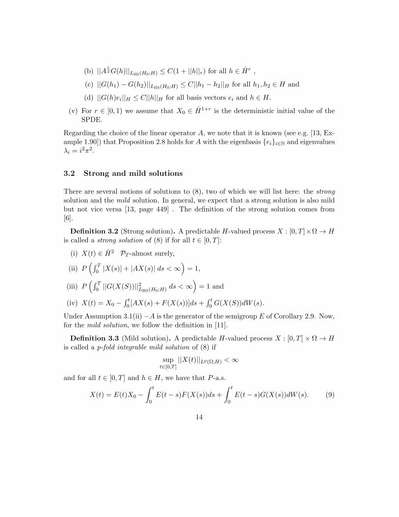
3.2 Strong and mild solutions

There are several notions of solutions to (8), two of which we will list here: the strongsolution and the mild solution. In general, we expect that a strong solution is also mildbut not vice versa [13, page 449] . The definition of the strong solution comes from[6].

Definition 3.2 (Strong solution). A predictable H-valued process X : [0, T ]×Ω→ His called a strong solution of (8) if for all t ∈ [0, T ]:

(i) X(t) ∈ H2 PT -almost surely,

(ii) P(∫ T

0 |X(s)|+ |AX(s)| ds <∞)

= 1,

(iii) P(∫ T

0 ||G(X(S))||2LHS(H0;H) ds <∞)

= 1 and

(iv) X(t) = X0 −∫ t

0 [AX(s) + F (X(s))]ds+∫ t

0 G(X(S))dW (s).

Under Assumption 3.1(ii) −A is the generator of the semigroup E of Corollary 2.9. Now,for the mild solution, we follow the definition in [11].

Definition 3.3 (Mild solution). A predictable H-valued process X : [0, T ]× Ω→ His called a p-fold integrable mild solution of (8) if

supt∈[0,T ]

||X(t)||Lp(Ω;H) <∞

and for all t ∈ [0, T ] and h ∈ H, we have that P -a.s.

X(t) = E(t)X0 −∫ t

0E(t− s)F (X(s))ds+

∫ t

0E(t− s)G(X(s))dW (s). (9)

14

This last definition is the one we will consider in this thesis, and in the next section, wecite an existence and uniqueness result.

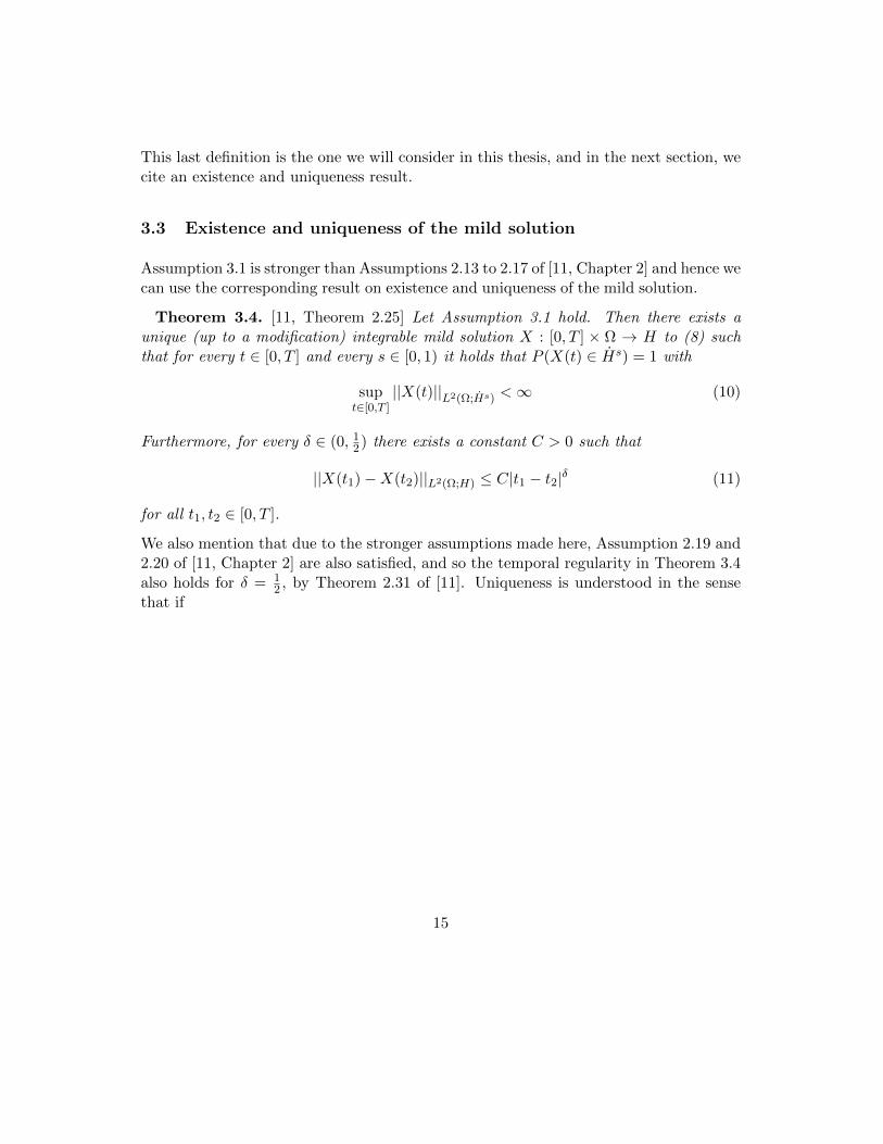
3.3 Existence and uniqueness of the mild solution

Assumption 3.1 is stronger than Assumptions 2.13 to 2.17 of [11, Chapter 2] and hence wecan use the corresponding result on existence and uniqueness of the mild solution.

Theorem 3.4. [11, Theorem 2.25] Let Assumption 3.1 hold. Then there exists aunique (up to a modification) integrable mild solution X : [0, T ] × Ω → H to (8) suchthat for every t ∈ [0, T ] and every s ∈ [0, 1) it holds that P (X(t) ∈ Hs) = 1 with

supt∈[0,T ]

||X(t)||L2(Ω;Hs) <∞ (10)

Furthermore, for every δ ∈ (0, 12) there exists a constant C > 0 such that

||X(t1)−X(t2)||L2(Ω;H) ≤ C|t1 − t2|δ (11)

for all t1, t2 ∈ [0, T ].

We also mention that due to the stronger assumptions made here, Assumption 2.19 and2.20 of [11, Chapter 2] are also satisfied, and so the temporal regularity in Theorem 3.4also holds for δ = 1

2 , by Theorem 2.31 of [11]. Uniqueness is understood in the sensethat if

15

4 Discretization methods for SPDE

In this chapter, we show how one can discretize the solution of (8) so that it can besimulated on a computer. From now on, we assume the conditions of Assumption 3.1and consider approximations of the mild solution. Throughout the sections 4.1 and 4.2we follow closely the approach of [11] but after that we leave this context and considerhow the covariance operator Q can be discretized.

4.1 Galerkin finite element methods

In this section, we briefly describe the Galerkin finite element method, which is our firststep in the discretization of (8). Here finite dimensional subspaces of H are considered,and so we speak of spatial discretizations.

Let (Vh)h∈(0,1] be a sequence of finite dimensional subspaces such that Vh ⊂ H1 ⊂ H.For these spaces, we follow the notation of [11] and consider two orthogonal projections:the usual Ph : H → Vh and the Ritz projection Rh : H1 → Vh. These are defined by therelations

〈Phx, yh〉H = 〈x, yh〉H for all x ∈ H, yh ∈ Vhand

〈Rhx, yh〉1 = 〈x, yh〉1 for all x ∈ H1, yh ∈ Vh.

As in [11, Chapter 3.2], we make the following assumptions on these projections:

Assumption 4.1. For the given family of subspaces (Vh)h∈(0,1] and all h ∈ (0, 1] thereexists a constant C such that

(i) ||Phx||1 ≤ C||x||1 for all x ∈ H1 and

(ii) ||Rhx− x||1 ≤ Chs||x||1 for all x ∈ Hs with s ∈ 1, 2.

We will consider an explicit choice of (Vh)h∈(0,1] later on. Next we introduce the discreteversion of the operator A, Ah : Vh → Vh. For each xh ∈ Vh we define Ahxh to be theunique element of Vh such that

〈Axh, yh〉H = 〈xh, yh〉1 = 〈Ahxh, yh〉H

for all yh ∈ Vh. By using this relation with the properties of the inner product 〈·, ·〉1one sees that Ah also is self-adjoint and positive definite on Vh. Therefore, as before, itis the generator of an analytic semigroup of contractions which we denote by Eh(t) and

16

one can show (see e.g. [11, Section 3.4]) that there exists a unique stochastic processXh : [0, T ]× Ω→ Vh which is the mild solution to the stochastic equation

dXh(t) +AhXh(t)dt = PhG(Xh(t))dW (t), for 0 ≤ t ≤ TXh(0) = PhX0.

This is called the semidiscrete approximation of the solution to (8), but we will notconsider it in detail in this thesis. The interested reader is referred to [11] for this.Instead, we will focus on the fully discrete approximation in which we also consider adiscretization with respect to time.

4.2 The implicit Euler scheme

In this section, we mirror the approach of [11, Section 3.5] who in turn draws from[19, Chapter 7]. We refer to these sources for more details and generalizations of ourinformal introduction to the implicit (or backward) Euler–Maruyama scheme.

Let again (Vh)h∈(0,1] be a sequence of finite dimensional subspaces such that for all

h ∈ (0, 1], Vh ⊂ H1 ⊂ H. Consider the homogenous equation

du(t) +Ahu(t)dt = 0

with inital value u(0) = u0 ∈ Vh for t > 0 and some fixed h ∈ (0, 1]. One can then show(see e.g. [19]) that the solution to this is given by the semigroup generated by −Ah,namely Eh(t). We may approximate this equation by defining the recursion

uj − uj−1 + kAhuj = 0, j ∈ N

for some fixed time step k ∈ (0, 1] where uj denotes the approximation of u(tj) withtj := jk. A closed form of this is then given by

uj = (I + kAh)−ju0, j ∈ N0

Now, following the notation of [11, Section 3.5] we write

Ek,h(t) := (I + kAh)−j if t ∈ [tj−1, tj) for j ∈ N

and we call this operator the rational approximation of the semigroup E(t) generatedby −A. We end this section by citing the following smoothing property of the scheme,from [11, page 67]:

||AρhEk,h(t)xh|| ≤ Ct−ρj ||xh|| (12)

which holds for any t ∈ [tj−1, tj), ρ ∈ [0, 1] and xh ∈ Vh.

17

4.3 A fully discrete strong approximation of the SPDE

In this section, we combine the Galerkin method with the linearly implicit Euler–Maruyama scheme and cite a convergence rate of the fully discrete approximation Xj

h

of X(tj), where X is the mild solution of (8).

For this, consider the same sequence of subspaces (Vh)h∈(0,1] as before and let T > 0 bethe fixed final time. Define a uniform timegrid with a time step k ∈ (0, 1] by tj = jk,j = 0, 1, ..., Nk with Nkk = T . Denote the fully discrete approximation of X(tj), where

X is the mild solution of (8), by Xjh. The recursion scheme that approximates X is

Xjh −X

j−1h + k(AhX

jh) = PhG(Xj−1

h )∆W j for j = 1, ..., Nk

X0h = PhX0

(13)

where ∆W j are the Wiener increments W (tj)−W (tj−1).

In terms of the operator Ek,h(t) one may equally well express this as

Xjh = Ek,h(tj−1)PhX0 +

∫ tj

0Ek,h(tj − s)PhGh(s) dW (s) (14)

where

Gh(s) :=

G(Xj−1

h ) if s ∈ (tj−1, tj ],

G(PhX0) if s = 0.

The following key theorem on convergence of the fully discrete approximation from [11]holds.

Theorem 4.2. [11, Theorem 3.14] Under Assumptions 3.1 with r ∈ [0, 1) and 4.1,for all p ∈ [2,∞) there exists a constant C independent of k, h ∈ (0, 1] such that

||Xjh −X(tj)||Lp(Ω;H) ≤ C(h1+r + k

12 ). (15)

4.4 Noise approximation

An issue remaining when one wants to simulate a realisation of X(t) for some t ∈ [0, T ]is how to simulate the Q-Wiener process W . We know that this can be expressed asan infinite sum of Brownian motions (see Theorem 2.19, the Karhunen–Loeve expan-sion), but we cannot simulate an infinite number of Brownian motions on the computer.

18

Therefore, if one wants to use this expansion, one needs to truncate it at some pointκ ∈ N. We then end up with a new Q-Wiener process:

W κ(t) =κ∑j=1

µ12j βj(t)ej

with the corresponding covariance operator Qκ defined by the relation

Qκej = 1j≤κµjej .

In the same way as before, we have a mild solution to (8) but now with truncated noise,and as in (14) it can be represented by

Xjκ,h = Ek,h(tj−1)PhX0 +

∫ tj

0Ek,h(tj − s)PhGκ,h(s) dW κ(s) (16)

where

Gκ,h(s) :=

G(Xj

κ,h) if s ∈ (tj−1, tj ]

G(PhX0) if s = 0.

We also introduce

W cκ(t) := W (t)−W κ(t) =∞∑

j=κ+1

µ12j βj(t)ej (17)

which also is a Q-Wiener process with covariance operator Qcκ = Q − Qκ. It can beseen that for the stochastic integral it holds∫ t

0φ(s)dW (s)−

∫ t

0φ(s)dW κ(s) =

∫ t

0φ(s)dW cκ(s).

In the following proof, we use these notions to give an error bound for Xjκ,h, c.f. Theo-

rem 4.2, when κ ∈ N is chosen appropriately, to reflect the decay η, of the eigenvaluesµj of Q, (see 3.1(i)). For this we take an approach that is very similar to the one foundin [2].

19

Theorem 4.3. Assume that Assumption 3.1 with r ∈ [0, 1) and Assumption 4.1

hold. Assume also that κ ' h−β for some β > 0. Furthermore, if h1+r ' k12 and

β(η − 1) = 2(1 + r), for all p ∈ [2,∞) it holds that

||X(tj)−Xjκ,h||Lp(Ω;H) ≤ Ch1+r.

for some constant C > 0.

Proof. Throughout this proof, we will use C to refer to any constant. First we split theerror, by using Lemma A.2:

||X(tj)−Xjκ,h||

2Lp(Ω;H) ≤ 2(||X(tj)−Xj

h||2Lp(Ω;H) + ||Xj

h −Xjκ,h||

2Lp(Ω;H))

=: 2(I + II)

For the first term, it holds that

I ≤ C(h1+r + k12 )2 ' Ch2(1+r) (18)

by Theorem 4.2. By Lemma A.2 and the representation of the fully discrete approxi-mation (14) and its truncated version (16) we have for II:∣∣∣∣∣∣∣∣∫ tj

0Ek,h(tj − s)PhGh(s) dW (s)−

∫ tj

0Ek,h(tj − s)PhGκ,h(s) dW k(s)

∣∣∣∣∣∣∣∣2Lp(Ω;H)

≤ 2

∣∣∣∣∣∣∣∣∫ tj

0Ek,h(tj − s)Ph(Gh(s)−Gκ,h(s)) dW (s)

∣∣∣∣∣∣∣∣2Lp(Ω;H)

+ 2∣∣∣∣∣∣∫ tj

0Ek,h(tj − s)PhGκ,h(s) dW (s)

−∫ tj

0Ek,h(tj − s)PhGκ,h(s) dW κ(s)

∣∣∣∣∣∣2Lp(Ω;H)

=: 2IIa + 2IIb

20

Now, by Theorem 2.21:

IIa = E[∣∣∣∣∣∣∣∣∫ tj

0Ek,h(tj − s)Ph(Gh(s)−Gκ,h(s)) dW (s)

∣∣∣∣∣∣∣∣pH

] 2p

≤ C E

[(∫ tj

0||Ek,h(tj − s)Ph(Gh(s)−Gκ,h(s))||2LHS(H0;H) ds

) p2

] 2p

= C E

(∫ tj

0

∑i∈N||Ek,h(tj − s)Ph(Gh(s)−Gκ,h(s))Qei||2H ds

) p2

2p

≤ C E

(∫ tj

0

∑i∈N||(Gh(s)−Gκ,h(s))Qei||2H ds

) p2

2p

= C E

[(∫ tj

0||(Gh(s)−Gκ,h(s))||2LHS(H0;H) ds

) p2

] 2p

≤ CE

(k j∑n=1

||Xn−1h −Xn−1

κ,h ||2H

) p2

2p

≤ Ckj∑

n=1

||(||Xn−1h −Xn−1

κ,h ||2H)||

Lp2 (Ω;R)

= Ck

j∑n=1

||Xn−1h −Xn−1

κ,h ||2Lp(Ω;R),

where the second inequality follows from the smoothing result (12) with ρ = 0, whilethe third follows from Assumption 3.1(iv)(c) and the fourth is the triangle inequality.For the other term, by the discussion preceeding this theorem and the representation(2) of (Qcκ)

12 :

IIb =

∣∣∣∣∣∣∣∣∫ tj

0Ek,h(tj − s)PhGκ,h(s) dW cκ(s)

∣∣∣∣∣∣∣∣2Lp(Ω;H)

≤ C E

[(∫ tj

0||Ek,h(tj − s)PhGκ,h(s)||2

LHS((Qcκ)12 [H];H)

ds

) p2

] 2p

= C E

(∫ tj

0

∞∑i=κ+1

µi||Ek,h(tj − s)PhGκ,h(s)ei||2H ds

) p2

2p

21

≤ C E

(∫ tj

0

∞∑i=κ+1

µi||Gκ,h(s)ei||2H ds

) p2

2p

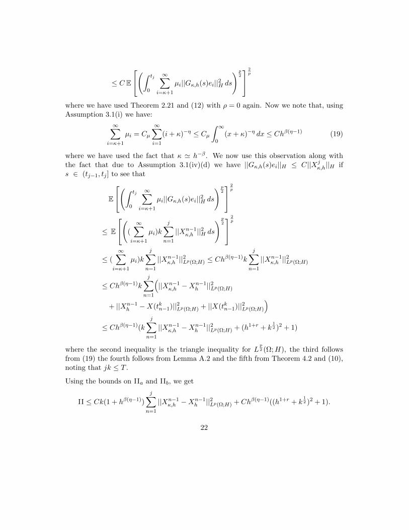
where we have used Theorem 2.21 and (12) with ρ = 0 again. Now we note that, usingAssumption 3.1(i) we have:

∞∑i=κ+1

µi = Cµ

∞∑i=1

(i+ κ)−η ≤ Cµ∫ ∞

0(x+ κ)−η dx ≤ Chβ(η−1) (19)

where we have used the fact that κ ' h−β. We now use this observation along withthe fact that due to Assumption 3.1(iv)(d) we have ||Gκ,h(s)ei||H ≤ C||Xj

κ,h||H ifs ∈ (tj−1, tj ] to see that

E

(∫ tj

0

∞∑i=κ+1

µi||Gκ,h(s)ei||2H ds

) p2

2p

≤ E

((

∞∑i=κ+1

µi)k

j∑n=1

||Xn−1κ,h ||

2H ds

) p2

2p

≤ (∞∑

i=κ+1

µi)k

j∑n=1

||Xn−1κ,h ||

2Lp(Ω;H) ≤ Ch

β(η−1)k

j∑n=1

||Xn−1κ,h ||

2Lp(Ω;H)

≤ Chβ(η−1)k

j∑n=1

(||Xn−1

κ,h −Xn−1h ||2Lp(Ω;H)

+ ||Xn−1h −X(tkn−1)||2Lp(Ω;H) + ||X(tkn−1)||2Lp(Ω;H)

)≤ Chβ(η−1)(k

j∑n=1

||Xn−1κ,h −X

n−1h ||2Lp(Ω;H) + (h1+r + k

12 )2 + 1)

where the second inequality is the triangle inequality for Lp2 (Ω;H), the third follows

from (19) the fourth follows from Lemma A.2 and the fifth from Theorem 4.2 and (10),noting that jk ≤ T .

Using the bounds on IIa and IIb, we get

II ≤ Ck(1 + hβ(η−1))

j∑n=1

||Xn−1κ,h −X

n−1h ||2Lp(Ω;H) + Chβ(η−1)((h1+r + k

12 )2 + 1).

22

Now we can use the discrete Gronwall inequality, Theorem A.1, with an = ||Xnκ,h −

Xnh ||2Lp(Ω;H) to get:

II ≤ Chβ(η−1)((h1+r + k12 )2 + 1)(1 + Ck(1 + hβ(η−1)))j

≤ Chβ(η−1)((h1+r + k12 )2 + 1)eCkj(1+hβ(η−1))

≤ Chβ(η−1)((h1+r + k12 )2 + 1)e2CT

= Chβ(η−1)((h1+r + k12 )2 + 1) ≤ Ch2(1+r),

where we have used that hα ≤ 1 for α > 0 and also the assumption β(η − 1) = 2(1 + r).Taken together with (18), we have the result.

23

5 Monte Carlo methods

In this chapter, we will describe how one can estimate quantities involving X(t). Westart by defining the two types of errors we will analyse. Throughout this chapter, weuse the notation Xj

κ,h to refer to the truncated fully discrete approximation definedin (16).

5.1 Strong and weak errors

We refer to the error ||X(tj) −Xjκ,h||L2(Ω;H) of Theorem 4.3 as the strong error of the

truncated fully discrete approximation Xjκ,h.

Often, one may not be interested in the paths of the solution to our SPDE (8) but ratherthe average value of some functional of its value at the final time T . Therefore, one isthen interested in the weak error

|E[φ(X(T )]− E[φ(XNkh,κ)]| (20)

where φ : H → R can be any sufficiently smooth test function.

In our case, we set Φ := || · ||2 and refer to the expression

|E[||X(T )||2H ]− E[||XNkh,κ||

2H ]| (21)

as the weak error of our truncated fully discrete approximation of X(T ).

Before we continue, we need to briefly mention the definition of a Frechet differentiableoperator.

Definition 5.1. Let B1 and B2 be Banach spaces and let U ⊆ B1 be an open set.A function φ : U → B1 is called Frechet differentiable at x ∈ U if there exists φ′(x) ∈L(B1;B2) such that

limh→0

||φ(x+ h)− φ(x)− φ′(x)h||B2

||h||B1

= 0.

Then φ′(x) is referred to as the Frechet derivative of φ at x ∈ U .

The weak error is weaker than the strong error in the sense that (as is mentioned in e.g.[11, page 3]):

|E[φ(X(T )]− E[φ(XNkh,κ)]| ≤ C||X(T )−XNk

κ,h||L2(Ω;H). (22)

24

This holds true when φ is Frechet differentiable and

||φ′(x)||L(H) ≤ C(1 + ||x||p−1H ).

Our choice of φ indeed fulfils this condition for all p ≥ 2, as:

||φ′(x)||L(H) = || 〈·, x〉H ||L(H) ≤ ||x||H

by the Cauchy–Schwarz inequality. Therefore, every strongly convergent approximationis also weakly convergent.

5.2 The Monte Carlo method

We first briefly review what the (ordinary) Monte Carlo method entails. Let (Yi)i∈N bea sequence of independent, identically distributed (i.i.d.) U -valued random variables,where U may be any Hilbert space. Then, for large enough N ∈ N, one could as in thereal case expect to have

EN (Y ) :=1

N

N∑i=1

Yi ≈ E [Y ] .

That this is true is made clear by the following. We cite a simple form of the law oflarge numbers that holds true in general Hilbert spaces.

Lemma 5.2. [4, Lemma 4.1] For N ∈ N and for Y ∈ L2(Ω;U) it holds that

||E [Y ]− EN [Y ]||L2(Ω;U) ≤1√N||Y ||L2(Ω;U).

Using this lemma, we can estimate the additional error when estimating the strong(L2-)error.

Proposition 5.3. Let the assumptions of Theorem 4.3 be fulfilled. Then, the MonteCarlo estimator with N ∈ N of ||X(tj)−Xj

κ,h||L2(Ω;H) satisfies∣∣∣∣∣∣∣∣EN [||X(tj)−Xjκ,h||

2H

] 12 − ||X(tj)−Xj

κ,h||L2(Ω;H)

∣∣∣∣∣∣∣∣L2(Ω;R)

≤ 1

N14

||X(tj)−Xjκ,h||L4(Ω;H).

25

Proof. We have that∣∣∣∣∣∣∣∣EN [||X(tj)−Xjκ,h||

2H

] 12 − ||X(tj)−Xj

κ,h||L2(Ω;H)

∣∣∣∣∣∣∣∣2L2(Ω;R)

=

∣∣∣∣∣∣∣∣EN [||X(tj)−Xjκ,h||

2H

] 12 − E

[||X(tj)−Xj

κ,h||2H

] 12

∣∣∣∣∣∣∣∣2L2(Ω;R)

≤∣∣∣∣∣∣∣∣∣∣∣EN [||X(tj)−Xj

κ,h||2H

]− E

[||X(tj)−Xj

κ,h||2H

]∣∣∣ 12 ∣∣∣∣∣∣∣∣2L2(Ω;R)

=∣∣∣∣∣∣EN [||X(tj)−Xj

κ,h||2H

]− E

[||X(tj)−Xj

κ,h||2H

]∣∣∣∣∣∣L1(Ω;R)

≤∣∣∣∣∣∣EN [||X(tj)−Xj

κ,h||2H

]− E

[||X(tj)−Xj

κ,h||2H

]∣∣∣∣∣∣L2(Ω;R)

≤ 1√N

E[||X(tj)−Xj

κ,h||4H

] 12

=1√N||X(tj)−Xj

κ,h||2L4(Ω;R),

where the first inequality follows from the fact that |√a −√b| ≤

√|a− b| for a, b ≥ 0.

The second inequality is the Holder inequality while the third follows from Lemma 5.2.

When it comes to the weak error, there are (at least) two ways of approximating it witha Monte Carlo method, namely∣∣∣E [||X(T )||2H

]− EN

[||XNk

h,κ||2H

]∣∣∣ (23)

and ∣∣∣EN [||X(T )||2H − ||XNkh,κ||

2H

]∣∣∣ . (24)

In practice, neither E[||X(T )||2H ] nor ||X(T )||2H will be known exactly, so one has toestimate them. However, there is an important distinction. The quantity E[||X(T )||2H ]

is a real number that can be estimated independently of EN

[||XNk

h,κ||2H

]while ||X(T )||2H

is a real-valued random variable that must be simulated using the same realisation ofthe Q-Wiener process as ||XNk

h,κ||2H . We will return to this in more detail in later sections.

For now, we prove the following result, analogously to Proposition 5.3.

26

Proposition 5.4. Let the assumptions of Theorem 4.3 be fulfilled. Then, the MonteCarlo estimators (23) and (24) with N ∈ N of |E[||X(T )||2H ]− E[||XNk

h,κ||2H ]| satisfy:∣∣∣∣∣∣|E [||X(T )||2H

]− EN

[||XNk

h,κ||2H

]| − |E

[||X(T )||2H − ||X

Nkh,κ||

2H

]|∣∣∣∣∣∣L2(Ω;R)

≤ C√N

(25)

and ∣∣∣∣∣∣|EN [||X(T )||2H − ||XNkh,κ||

2H

]| − |E

[||X(T )||2H − ||X

Nkh,κ||

2H

]|∣∣∣∣∣∣L2(Ω;R)

≤ C√N

∣∣∣∣∣∣X(T )−XNkκ,h

∣∣∣∣∣∣L2(Ω;H)

.(26)

Proof. By the reverse triangle inequality, the left hand side of (25) is bounded by

||E[||XNk

h,κ||2H

]− EN

[||XNk

h,κ||2H

]||L2(Ω;R). The inequality now follows from Lemma 5.2

and the fact that ||XNkh,κ||L2(Ω;H) ≤ C < ∞ for some C > 0, which in turn is a conse-

quence of Theorem 4.3 and (10).

Next, we again use the reverse triangle inequality to see that the left hand side of (26)is bounded by∣∣∣∣∣∣EN [||X(T )||2H − ||X

Nkh,κ||

2H

]− E

[||X(T )||2H − ||X

Nkh,κ||

2H

]∣∣∣∣∣∣L2(Ω;R)

≤ 1√N

∣∣∣∣∣∣||X(T )||2H − ||XNkh,κ||

2H

∣∣∣∣∣∣L2(Ω;R)

=1√N

∣∣∣∣∣∣⟨X(T ) +XNkh,κ, X(T )−XNk

h,κ

⟩H

∣∣∣∣∣∣L2(Ω;R)

≤ C√N

∣∣∣∣∣∣X(T )−XNkh,κ

∣∣∣∣∣∣L2(Ω;H)

Here, the first inequality follows from Lemma 5.2, while the second follows from theCauchy–Schwarz inequality along with the fact that ||XNk

h,κ||L2(Ω;H) ≤ C < ∞ and||X(T )||L2(Ω;H) ≤ C <∞ for some C > 0.

27

5.3 The Multilevel Monte Carlo method

One problem with the Monte Carlo estimator of the strong and weak errors describedin the previous section is the large number of samples needed for a good estimate. Thisis not a problem when the approximation in time and space is rough, since it is compu-tationally relatively cheap. However, this estimator has a high bias. A compromise isnot to solve all samples on the same discretization level - we want to generate a largenumber of samples on a coarse grid and fewer samples on a fine grid and then add themtogether to get an estimator that has both low variance and bias and is computationallycheaper than the estimator EN (Y ), which we from now on will refer to as the singlelevelMonte Carlo estimator. In this section, we introduce the multilevel Monte Carlo in ageneral framework, similar to that of [3].

Assume that (Y`)`∈N0 is a sequence of approximations of the U -valued random variableY , where we have denoted the set of non-negative integers by N0 as opposed by the setof positive integers which we denote by N. For any L ∈ N it holds that

YL = Y0 +

L∑`=1

(Y` − Y`−1)

and by the linearity of the expectation operator

E [YL] = E [Y0] +

L∑l=1

E [(Y` − Y`−1)] . (27)

This motivates the multilevel Monte Carlo estimator

EL[YL] := EN0 [Y0] +L∑`=1

EN`(Y` − Y`−1)

where EN`(Y` − Y`−1) is the singlelevel Monte Carlo estimator with a number of inde-pendent samples N` depending on the level `.

We prove the following slightly modified version of [3, Lemma 2.2].

Lemma 5.5. Let (Y`)l∈N0 be a sequence of approximations to Y ∈ L2(Ω,R) andassume further that Y` ∈ L2(Ω;R) for all ` ∈ N0. Then it holds that

||E [Y ]− EL[YL]||L2(Ω,R)

≤ |E [Y − YL] |+

(1

N0||Y0||2L2(Ω;R) +

L∑l=1

1

N`||Y` − Y`−1||2L2(Ω;R)

) 12

28

Proof. By the triangle inequality

||E [Y ]− EL[Y ]||L2(Ω,R) ≤ ||E [Y ]− E [YL] ||L2(Ω,R) + ||E [YL]− EL[YL]||L2(Ω,R)

= |E [Y − YL] |+ ||E [YL]− EL[YL]||L2(Ω,R).

For the second term, we have using the telescoping sum at the right hand side of (27),

||E [YL]− EL[YL]||2L2(Ω,R)

= ||E [Y0]− EN0 [Y0] +L∑l=1

(E [Y` − Y`−1]− EN` [Y` − Y`−1])||2L2(Ω,R)

= ||E [Y0]− EN0 [Y0]||2L2(Ω,R) +

L∑l=1

||(E [Y` − Y`−1]− EN` [Y` − Y`−1])||2L2(Ω,R),

where the last equality follows from the linearity of the ||·||2L2(Ω;R)-operator for real-valuedindependent zero-mean random variables. The result now follows from Lemma 5.2.

We now make an explicit application of this multilevel Monte Carlo estimator. Recallingthe notation and setting of Theorem 4.3, we set h` = h02−` for ` ∈ N0 with some real

h0 > 0. Let X` := XNk`κ`,h`

where k` = h2` and κ` = h

2η−1

` . Then we get a series of

H-valued random variables such that X` ∈ L2(Ω, H), and by Theorem 4.3, for all p ≥ 2there exists a constant C > 0 independent of h`, κ` and k` such that:

||X` −X(T )||L2(Ω;H) ≤ Ch` = Ch02−`. (28)

We now apply Lemma 5.5 to this sequence of H-valued random variables.

Proposition 5.6. Let X` := XNk`κ`,h`

where for some real h0 > 0, h` = h02−`, k` = h2`

and κ` = h2

η−1

` . Let δ > 0 and for ` ≤ L with L, ` ∈ N0 let N` of the multilevel estimator

EL fulfil N` ' h2(1−α)0 `1+δ22(αL−`) for ` ≥ 1 and N0 ' h−2α

0 22αL. Assuming that thereexists constants C1, α > 0 such that for all ` ∈ N0 the weak error satisfies

|E[||X(T )||2H − ||X`||2H

]| ≤ C1h

α0 2−α`,

then there exists a constant C2 not depending on L such that

||E[||X(T )||2H

]− EL[||XL||2H ]||L2(Ω,R) ≤ C2h

α0 2−αL.

29

Proof. By Lemma 5.5 we have

||E[||X(T )||2H

]− EL[||XL||2H ]||L2(Ω,R)

≤ |E[||X(T )||2H − ||XL||2H

]|

+ C

(1

N0||X0||4L4(Ω;R) +

L∑l=1

1

N`

∣∣∣∣∣∣||X`||2H − ||X`−1||2H∣∣∣∣∣∣2L2(Ω;R)

) 12

.

Furthermore,∣∣∣∣∣∣||X`||2H − ||X`−1||2H∣∣∣∣∣∣2L2(Ω;R)

=∣∣∣∣∣∣⟨X` + X`−1, X` − X`−1

⟩H

∣∣∣∣∣∣2L2(Ω;R)

≤ C∣∣∣∣∣∣X` − X`−1

∣∣∣∣∣∣2L2(Ω;H)

≤ 2C

(∣∣∣∣∣∣X(T )− X`

∣∣∣∣∣∣2L2(Ω;H)

+∣∣∣∣∣∣X(T )− X`−1

∣∣∣∣∣∣2L2(Ω;H)

)≤ Ch2

0(2−2` + 2−2(`−1)) = Ch20(2−2` + 4 · 2−2`) ≤ Ch2

02−2`,

where the first inequality follows from the Cauchy–Schwarz inequality and the fact thatthe truncated fully approximations are bounded (c.f. the proof of Proposition 5.4). Thesecond inequality is Lemma A.2 while the third is the convergence rate of the strongerror, as outlined above. Therefore, using the fact that the truncated fully discreteapproximations are bounded once again:

1

N0||X0||4L4(Ω;R) +

L∑`=1

1

N`

∣∣∣∣∣∣||X`||2H − ||X`−1||2H∣∣∣∣∣∣2L2(Ω;R)

≤ C

(1

N0+

L∑`=1

1

N`h2

02−2`

)≤ Ch2α

0

(2−2αL + 2−2αL

L∑`=1

`−(1+δ)

)≤ Ch2α

0 (1 + ζ(1 + δ))2−2αL ≤ Ch2α0 2−2αL,

where ζ denotes the Riemann zeta function. Summing up, using the assumption on theweak convergence, we get our result

||E[||X(T )||2H

]− EL[||XL||2H ]||L2(Ω,R)

≤ C(hα0 2−αL + (h2α0 2−2αL)

12 ) ≤ Chα0 2−αL.

We remark that the assumption on the weak convergence rate of Proposition 5.6 holdstrue at least for α = 1 since the weak error is bounded by the strong error.

30

6 Simulations

In this chapter, some numerical experiments in connection to the results of the previouschapters will be described. We will focus on the simulation of the strong and weakapproximation errors.

However, we start by defining two noise operators (the term G in (8)), G1 and G2,which, we recall, are functions on H = L2([0, 1];R) taking values in LHS(H0;H).

6.1 Geometric Brownian motion in infinite dimensions

The first operator G1 is taken from [11, Section 6.4]. For h ∈ H and h0 ∈ H0 it isdefined by

G1(h)h0 :=

∞∑j=1

〈h, ej〉H 〈h0, ej〉H ej .

We have to check the conditions of Assumption 3.1(iv) to see that they hold. To seethat for all h ∈ H, G1(h) ∈ LHS(H0; Hr), note that

||G1(h)||LHS(H0;Hr) = ||Ar2G1(h)||LHS(H0;H) ≤ tr(Q)

12 ||A

r2G1(h)||L(H)

by Lemma 2.22 and that by Lemma 2.3

||Ar2G1(h)||2L(H) ≤ ||A

r2G1(h)||2LHS(H) =

∞∑i=1

||Ar2 〈h, ei〉H ei||

2H

=∞∑i=1

||Ar2 〈h, ei〉H ei||

2H =

∞∑i=1

||λr2i 〈h, ei〉H ei||

2H

=∞∑i=1

λri 〈h, ei〉2H = ||h||2r

using Parseval’s identity and Proposition 2.8. Therefore for all r ≥ 0 we have

||G1(h)||LHS(H0;Hr) ≤ tr(Q)||h||r,

which shows the first two assumptions of Assumption 3.1(iv) - the third also followsfrom this since for h1, h2 ∈ H:

||G(h1)−G(h2)||LHS(H0;H) = ||G(h1 − h2)||LHS(H0;H)

≤ tr(Q)||h1 − h2||H .

31

Finally, the fourth assumption follows from the fact that the ONB of H (see Assump-tion 3.1(i)) is uniformly bounded.

Now, this choice of G admits an analytical solution of (8), as is shown in [11, Section6.4] - for t ∈ [0, T ] we get

X(t) =

∞∑i=1

〈X0, ei〉H exp

(−(λi +

µi2

)t+ µ12i βi(t)

)ei. (29)

So on each basis function of H, the process follows a geometric Brownian motion, whichis the reason for the name of this section and this process.

Since βi(T ) ∼ N(0, T ), it is easy to show that E[exp

(2µ

12i βi(T )

)]= exp (2µiT ) and

so by Parseval’s identity we have

E[||X(T )||2H

]=

∞∑i=1

〈X0, ei〉2H exp (−(2λi + µi)T ) . (30)

6.2 The heat equation with multiplicative Nemytskii-type noise

The next operator G2 is analysed in detail in [10]. For this, we let γ : R → R be aLipschitz continuous function and we then define G2 : H → LHS(H0;H) for h ∈ H,h0 ∈ H0 and x ∈ [0, 1] by

(G2(h)h0)[x] := γ(h(x))h0(x).

As it is noted in [11, Example 2.23], the analysis of [10, Section 4] shows that G2 isglobally Lipschitz and that there furthermore exists a constant C > 0 such that forh ∈ H

||G2(h)||LHS(H0;H) ≤ C tr(Q) (1 + ||h||H)

and under the additional assumption

∞∑i=1

µi supx∈[0,1]

|e′i(x)|2 <∞ (31)

there exists a constant C > 0 such that

||Ar2G(h)||LHS(H0;H) ≤ C(1 + ||h||r)

32

for all r ∈ [0, 12) and h ∈ Hr. Since e′i(x) =

√2iπ cos(iπx), (31) holds if η > 3. This

shows the first three assumptions of Assumption 3.1(iv) for any r ∈ [0, 12) while the last

one again follows from the uniform bound of the ONB of H. In the remainder of thethesis we take γ(x) to be sin(x).

6.3 Simulation setting

In the next few sections, we will use the single level Monte Carlo method to simulateboth strong and weak error rates and use the multilevel Monte Carlo method to simulateweak error rates of the equation (8). The computations will be done in MATLAB, inpart on a desktop computer and in part on a computer cluster.

We now consider equidistant partitions in space on the domain [0, 1] with h = 1Nh

,xj := jh, j = 0, 1, 2, ..., Nh. For each such partition we let Vh be given by the set ofall continuous functions on [0, 1] that are piecewise linear on the intervals [xj , xj+1] forj = 0, 1, 2, ...Nh−1 and zero at the boundary of the domain. From [11, Example 3.6] wesee that this choice of Vh fulfils Assumption 4.1. The sequence of hat functions (Φj)

Nh−1j=1

defined by their nodal values

Φj(xi) =

1, if i = j,

0, if i 6= j

forms a basis for Vh.

We will compute the numerical approximations XNkκ,h by recursively solving the numerical

equation

Xjκ,h −X

j−1κ,h + k(AhX

jκ,h) = Ghi (Xj−1

κ,h )∆W κ,j for j = 1, ..., Nk

X0κ,h = IhX0.

(32)

where ∆W κ,j are the Wiener increments W κ(tj) − W κ(tj−1) and the interpolationoperator Ih : H → Vh is defined by

Ihf(x) =

Nh−1∑j=1

f(xj)Φj(x)

and for Ghi : Vh → LHS(H0;Vh), i ∈ 1, 2 we set

Gh1(v)[h0] :=κ∑i=1

〈v, Ihei〉H 〈Ihh0, Ihei〉H Ihei

33

andGh2(v)[h0] := IhG2(v)Ihh0.

We do not exactly know how or if these changes of projections from Ph to differentconstellations of interpolation operators Ih affect the order of convergence. However,this kind of replacement of projectors seems to be quite common in practice and theymake the computation easier. We leave this choice unjustified, subject to future re-search.

We now fix η = 5, T = 1 and for ` ∈ N0 we set h` = 2−`, k` = h2` and κ` = h−1

` to get a

series of solutions to (32) which we denote by X` := XNk`κ`,h`

. We note that by our choice

of η it would have been sufficient to set κ` = h−1/2` and still have, by Theorem 4.3 with

r = 0,||X(T )− X`||L2(Ω;H) ≤ 2−` (33)

but for computational reasons we abstain from this and note that still (33) holds with thischoice. We also set X0(x) := x−x2 and note that this satisfies Assumption 3.1(v).

We end this section by remarking that in practice, given a finite element space Vh, we

will estimate the norm in H by ||f ||H ≈√∑Nh−1

j=1 |f(xj)|2.

6.4 Results: Strong convergence rates

We start by using the singlelevel Monte Carlo estimator to try to estimate the strongerror rate. When we say that the strong error converges with a rate of α, we mean inthis context that there exists a constant C > 0 such that

||X(T )− X`||L2(Ω;H) ≤ Chαl = C2−αl. (34)

In general, when simulating the quantity on the left hand side of this expression, we donot have access to the exact value of X(T ) for a given realisation of X. This is true evenwhen, for the case of G = G1, we can use the expression (29) for t = T , since we cannotgenerate an infinite number of Brownian motions. Instead, we use a so called referencesolution, that is, we replace the expression ||X(T ) − X`||L2(Ω;H) by ||XL − X`||L2(Ω;H)

where we let XL = XL for L > ` when we consider G = G2 while we let XL be givenby the expression (29) truncated at κL = 2L when we consider the case G = G1.

Now we investigate the strong rate of convergence for different choices of Cµ, whichinfluence the overall level of variance in the realisations of X (recall that the eigenvalues

34

of Q are µi = Cµi−5). For M = 2 · 104, ` = 1, 2, 3, 4, 5 and L = 6 we compute the

quantities

EM

[||XL − X`||2H

] 12

for G1 and G2. Informed by Proposition 5.3 we hope that these will approximate thestrong error well.

In Figure 1 we plot these values against 2` for ` = 1, 2, 3, 4, 5 where we use a logarithmicscale for both axes: a so called log-log plot. By [18] it holds that in this graph aconvergence of order α corresponds to a line with slope −α.

It should be noted that given a fixed Cµ all observations of XL and X` are computedon the same M instances of Q-Wiener processes W κL . Therefore, the variance will bemuch lower than if we for each level ` had generated X` independently of the other levels.Also, the same set of Q-Wiener processes was used for the strong error corresponding toG1 and the strong error corresponding to G2, so in Figure 1 the paths are independentof one another with respect to different values of Cµ, but for the same value of Cµ apath in the lower picture is not independent of the corresponding path in the upperpicture.

The theoretical results of Chapters 3 and 4 make us expect a convergence rate of order 1as noted in (34). Furthermore, when Cµ = 0, the equation reduces to the deterministiccase, and from [12, Chapter 10] we expect a convergence of order 2 in this case. Theresults of Figure 1 seem to be more or less in line with this. For small values of Cµwe appear to get a rate of order 2 but asymptotically it seems reasonable to expect aconvergence of order 1 in this case. When Cµ > 10 the variance is so great that thecurves appear very erratic, despite the use of a single set of Q-Wiener processes for alllevels `.

Next, we choose to look more closely at how the strong convergence behaves whenCµ = 10, so we take levels ` up to ` = 7 with L = 8 and set M = 3 · 103. Despite therelatively low number of samples, this computation takes a very long time if we were torun it on a typical desktop computer.

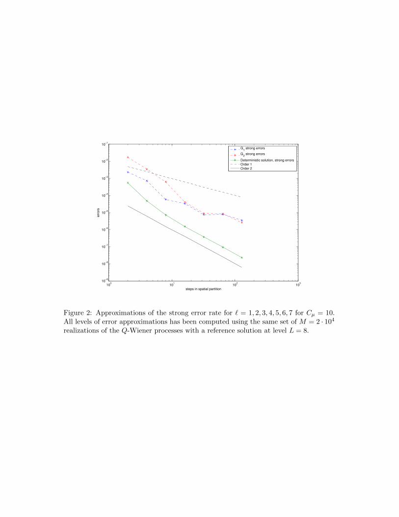
Fortunately, we have access to the Glenn cluster at Chalmers Centre for ComputationalScience and Engineering (C3SE). The system consists of 379 compute nodes with a totalof 6080 cores [17]. With ` and M as above, the total computation for all levels takes10 hours and 32 seconds using 8 computing nodes with 128 cores. The result is shownin Figure 2. From this we can see that the trend of a convergence of order 1 seems tohold, even with this somewhat low number of samples.

35

100

101

102

10−8

10−7

10−6

10−5

10−4

10−3

10−2

10−1

100

steps in spatial partition

str

ong e

rrors

Order 1

Order 2

Deterministic equationC

mu=1

Cmu

=3

Cmu

=10

Cmu

=20

Cmu

=30

Cmu

=40

100

101

102

10−8

10−7

10−6

10−5

10−4

10−3

10−2

10−1

100

steps in spatial partition

str

ong e

rrors

Order 1

Order 2

Deterministic equationC

mu=1

Cmu

=3

Cmu

=10

Cmu

=20

Cmu

=30

Cmu

=40

Figure 1: Approximations of the strong error rate for ` = 1, 2, 3, 4, 5 and different valuesof Cµ. The upper image shows the case G = G1 and the lower image G = G2. Foreach Cµ, all levels of error approximations have been computed using the same set ofM = 2 · 104 realisations of the Q-Wiener processes.

To utilize the resources of the cluster in an optimal way, it is crucial to make sure thatthe code can run in parallel. In our case, this essentially amounts to changing the forloop of our Monte Carlo computation to a so called parfor loop, which is a feature of theMATLAB Distributed Computing Server, installed on the cluster. In the user manualof the Parallel Computing Toolbox [15] we can read:

A parfor-loop is useful in situations where you need many loop iterationsof a simple calculation, such as a Monte Carlo simulation. parfor divides theloop iterations into groups so that each worker executes some portion of thetotal number of iterations. parfor-loops are also useful when you have loopiterations that take a long time to execute, because the workers can executeiterations simultaneously.

From this manual we also note that each worker is assigned a unique random numberstream so we can be sure that we are getting M independent samples of the Q-Wienerprocess.

The code used to produce the results of Figure 1 and 2 can be found in Section B.

6.5 Results: Weak convergence rates

Next, we compare the strong convergence rates to the weak rates. These are definedcompletely analogously to how we defined the strong rate in (34). To our knowledge,no simulations of the weak convergence rates of fully discrete approximations (usingthe FEM) of SPDE with multiplicative noise have been published, so this could be ofinterest for future research. A common ”rule of thumb” (see e.g. the introduction of[11]) within this field is that the weak rate of convergence is twice that of the strongrate. Therefore, in particular we investigate whether one can achieve a rate of order 2in the same context as the previous simulation, that is, when we consider ` from 1 to 7,L = 8 and we take M = 3 · 103.

Now, as we recall from Section 5 there are (at least) two ways of approximating it witha Monte Carlo method, namely∣∣∣E [||XL||2H

]− EM

[||X`||2H

]∣∣∣and ∣∣∣EM [||XL||2H − ||X`||2H

]∣∣∣ .which we refer to as the weak error rate of type I and type II respectively.

37

100

101

102

103

10−9

10−8

10−7

10−6

10−5

10−4

10−3

10−2

10−1

steps in spatial partition

err

ors

G

1 strong errors

G2 strong errors

Deterministic solution, strong errors

Order 1

Order 2

Figure 2: Approximations of the strong error rate for ` = 1, 2, 3, 4, 5, 6, 7 for Cµ = 10.All levels of error approximations has been computed using the same set of M = 2 · 104

realizations of the Q-Wiener processes with a reference solution at level L = 8.

For the weak error of type I we choose to estimate the quantity E[||XL||2H

]for the case

G = G1 by the deterministic quantity

106∑i=1

〈X0, ei〉2H exp (−(2λi + µi)) (35)

since we have access to the analytical solution as expressed in (30). For the case of

G = G2 we do not have this, so we instead estimate E[||XL||2H

]by EM

[||XL||H

]. In

this case we will estimate E[||XL||2H

]on a different set of Q-Wiener processes than that

used to generate EM

[||X`||2H

].

For the weak error of type II we generate both ||XL||2H and ||X`||2H on the same set ofQ-Wiener processes where we again make use of (29) truncated at κ = h−1

L and h−1`

respectively to generate these in the case of G = G1. The resulting simulation is shownin Figure 3. In this case we see that the error is much smaller than when we simulatedthe strong error in Figure 2 which is what we expect. However, it is hard to gauge anyparticular rate of convergence since the variance seems to dominate the weak error rate.We also note that we appear to have no rate of convergence at all when we consider thecase G = G1 and an independent (in this case deterministic) reference solution, an issuethat we will return to shortly. For G = G2, the addition of an independent estimateof the reference solution seems to have little to no influence on the behaviour of thesimulation of the weak rate of convergence. The behaviour of the last two points couldbe due to the fact that we consider a reference solution at the next (L=8) level insteadof taking the exact solution. The computation to create this picture takes 19 hours, 59minutes and 32 seconds using 8 computing nodes with 128 cores.

In Figure 4 we repeat these simulations for Cµ = 5. We note that we get clearer indica-tions of a rate of convergence which is somewhere between a rate of 1 and 2. We now also

include the case of the type I error when all of the approximations of EM

[||X`||2H

]are

independent of one another. In this case we have increased M to 105, but despite this,the noise is so great that it is impossible to say anything about the order of convergence.The computation time for these is presented in Table 1.

Remark 6.1. The complete lack of convergence in the case of a deterministic referencesolution in Figure 3 needs to be addressed. To do this purpose we can use the fact that

we have an analytical expression of X(T ) to investigate the behaviour of EM

[||XL||2H

]39

100

101

102

103

10−13

10−12

10−11

10−10

10−9

10−8

10−7

10−6

10−5

10−4

10−3

steps in spatial partition

err

ors

Order 2G

2 weak errors. independent reference solution

G2 weak errors

G1 weak errors. independent reference solution

G1 weak errors

Deterministic solution, weak errors

Figure 3: Approximations of the weak error rate for ` = 1, 2, 3, 4, 5, 6, 7 and Cµ = 10.In one set of cases the reference solution has been generated on an independent setof Q-Wiener processes and in one set it has been generated on the same set as theobservations for the levels ` = 1, 2, 3, 4, 5, 6, 7.

Level ` Time for G = G1 Time for G = G2

2 00:01:28 00:00:49

3 00:01:09 00:00:38

4 00:00:51 00:00:51

5 00:02:31 00:02:14

6 00:21:09 00:16:28

7 07:13:20 04:57:38

Table 1: Time needed to compute the independent weak error estimates in Figure 4using 8 computing nodes with 128 cores. The time for ` = 1 was not recorded. 105

samples were taken at each level.

100

101

102

103

10−12

10−11

10−10

10−9

10−8

10−7

10−6

10−5

10−4

steps in spatial partition

weak e

rrors

Order 2G

2 weak errors. independent reference solution

G2 weak errors

G1 weak errors. independent reference solution

G1 weak errors

G2 independent estimates at each level

G1 independent estimates at each level

Figure 4: Approximations of the weak error rate for ` = 1, 2, 3, 4, 5, 6, 7 and Cµ = 5. Forthe lines: in one set of cases the reference solution has been generated on an independentset of Q-Wiener processes and in one set it has been generated on the same set as theobservations for the levels ` = 1, 2, 3, 4, 5, 6, 7. For the dots: all weak error estimateshave been generated on independent sets of 105 Q-Wiener processes with a referencesolution generated at L = 8 using 104 Q-Wiener processes.

when M is large and L = 8. Using (29) and the fact that for all i ∈ N, βi(T ) ∼ N(0, 1),we estimate ||XL||2H by

||NhL∑i=1

〈X0, ei〉H exp

(−(λi +

µi2

) + µ12i Zi

)IhLei||

2H

where Zi ∼ N(0, 1) i.i.d. and we use this to compute EM

[||XL||2H

]which we plot

against M ranging from 1 to 106 in Figure 5 (note that for an increase in M we justadd another observation of ||XL||2H as opposed to generating another M + 1 number

of observations). We see that for the final value of M the value of EM

[||XL||2H

]is

almost entirely attributable to one single observation of ||XL||2H . This indicates that thedistribution is highly skewed, so that a large number of observations will be very close tozero but the sample mean will be much larger due to the presence of very large outliers.

Another (not entirely rigorous) way to think about this is to realize that since 〈X0, ei〉2Hdecreases rapidly with increasing values of i and λi + µi

2 is increasing in i, we shouldoften have

||NhL∑i=1

〈X0, ei〉H exp

(−(λi +

µi2

) + µ12i Zi

)IhLei||

2H

≈ || 〈X0, e1〉H exp

(−(λi +

µ1

2) + µ

121 Z1

)IhLe1||2H

which has a log-normal distribution. A well-known fact of the log-normal distribution isthat it is highly skewed to the right when the variance of the underlying normal distributedvariable (in this case µ1Z1) is big, so we should expect the presence of a small numberof very large outliers which in turn means that in the majority of cases, for reasonable

values of M , EM

[||XL||2H

]will be relatively far from the true mean.

6.6 Results: Multilevel Monte Carlo estimations

We end our numerical exploration by implementing the multilevel Monte Carlo estimatorfor the weak error. As in Figure 4 we let Cµ = 5 and for ` = 0, 1, 2, ... we set h` = h02−`,

k` = h2` and κ` = h−1

` to get a series of solutions to (32) which we denote by X` := XNk`κ`,h`

.

For computational reasons we let h0 = 2−1.

42

0 1 2 3 4 5 6 7 8 9 10

x 105

0

0.1

0.2

0.3

0.4

0.5

0.6

0.7

0.8

0.9

1x 10

−6

number of samples

estim

ate

of L

2 n

orm

Figure 5: A plot of EM [||X8||2H ] for M ranging from 1 to 106.

Let us make the bold assumption that the weak error rate actually is twice that of thestrong error rate. Then we have

|E[||X(T )||2H − ||X`||2H

]| ≤ C1h

202−2`

and so, from Proposition 5.6 we get

||E[||X(T )||2H

]− EL[||XL||2H ]||L2(Ω,R) ≤ C2h

202−2L.

Let us now test this for L = 1, 2, 3, 4, 5. As in Section 6.5, we replace E[||X(T )||2H

]by (35) in the case of G = G1 and in the case of G = G2 we replace it by a referencesolution EM [||X7||2H ] where we let M = 104. We generate all quantities independently

of one another, but when computing a single multilevel estimate EL[||XL||2H it is vital

to let the differences ||X`||2H − ||X`−1||2H be computed on the same Q-Wiener process.In the case of G = G1, the total computation time for all levels was 10 minutes and39 seconds and in the case of G = G2, the total computation time was 9 minutes. Thecomputation time is thus reduced by more than a factor of two when compared to takingM = 105 in the singlelevel estimator.

The errors∣∣∣E [||X(T )||2H

]− EL[||XL||2H ]

∣∣∣ are shown in the upper part of Figure 6. For

comparison purposes, we have also included the independent weak errors from Figure 4.We note that for both noise operators, we are able to achieve similar results to a smallercomputational cost using the multilevel estimator. In the lower part of Figure 6 we takethe L2-average of 100 realizations of the multilevel algorithm, that is we plot

E100

[∣∣∣E [||X(T )||2H]− EL[||XL||2H ]

∣∣∣2] 12

and we see that we get an order of convergence which is very close to 2.

6.7 Concluding discussion

In the numerical experiments outlined above, we first tried to simulate the strong rate ofconvergence predicted by the theory of the previous chapters of this thesis. The resultsseem to be consistent with this theory, although the noise makes it hard to say anythingfor certain about this.

In the case of weak convergence, we noted that when we tried to estimate the weakerrors using the same set of Q-Wiener processes there were indications that the rule of

44

100

101

102

10−9

10−8

10−7

10−6

10−5

10−4

10−3

steps in spatial partition

weak e

rrors

Order 2G

2 weak errors, multilevel estimates

G1 weak errors, multilevel estimates

G2 independent estimates at each level

G1 independent estimates at each level

100

101

102

10−9

10−8

10−7

10−6

10−5

10−4

10−3

steps in spatial partition

weak e

rrro

s

G1 weak errors, average multilevel estimates

G2 weak errors, average multilevel estimates

Order 2

Figure 6: Upper picture: A comparison between multilevel estimates computed at ` =1, 2, 3, 4, 5 and the corresponding (single level) weak errors where each level is simulatedindependently of one another of Figure 4. Lower picture: Two L2 averages of 100realisations of the multilevel schemes of the upper picture.

thumb stating that the weak rate often is twice the strong rate seemed to hold. However,especially in the analytical case, when comparing the estimates to a reference solutionwhich had been computed independently of these, the pattern was not very clear. Whenwe finally had all the estimates computed independently of one another there were closeto no indications of convergence, despite the relatively expensive computations. Thisshows how it, even in these relatively simple cases, can be hard to actually estimatequantities of the solution in practice due to the variance of these, and perhaps due toproperties of their distribution as well.

However, in the case of the multilevel estimates, we were able to get a rate of convergencethat seems to be close to 2 despite having each level estimate be independent of oneanother. The pattern was much clearer, though, when an average of multiple runs of themultilevel algorithm was taken. We stress, though, that the application of the multilevelalgorithm assumes that the weak rate of convergence actually is two, something that wehave not provided theory for. The result nevertheless shows the practical value of themultilevel algorithm and together with the results on the singlelevel weak error rates,may indicate some interesting directions for future research.

46

A Appendix

This appendix contains two useful inequalities that do not fit in well elsewhere. Westart with the following discrete Gronwall inequality from [5].

Lemma A.1. [5, page 280] Let (an)n∈N, (bn)n∈N and (cn)n∈N be non-negative se-quences such that

an ≤ bn +n−1∑k=0

ckak

for n ≥ 0. Then

an ≤ maxθ∈0,1,...,n

bθ

n−1∏k=0

(1 + ck)

The second result is an arithmetic inequality which we use in several places throughoutthe thesis and prove below.

Lemma A.2. Let n ∈ N and let ai, i = 1, 2, ...n be non-negative numbers. Then(n∑i=1

ai

)p≤ np−1

n∑i=1

api

Proof. Consider the measure space (Ω,A, µc) with Ω = 1, 2, ..., n,A = P(Ω), the power set of Ω, and µc being the counting measure. Let f, g : Ω→ R bedefined by f(k) = 1 and g(k) = ak. Then, by Holder’s inequality:

n∑i=1

ai = ||fg||1 ≤ ||f ||q||g||p = n1q

(n∑i=1

api

) 1p

where p−1 + q−1 = 1. The result now follows by raising each side of the inequality tothe p-th power.

47

B Source code

B.1 HSHE strong errors

This function is used to produce the results of Figure 1 and 2.

function [strong errors G1, ...strong errors G2]=HSHE strong errors(maximum ell, M, eigenconstant, ...eigendecay)

% Produces the strong error approximations for the homogeneous of Figure X.% Uses M realizations of the $Q$-Wiener process with% Qe j=eigenconstant*jˆ(-eigendecay) to compute approximations for h% ranging from 2ˆ-1 to 2ˆ-maximum ell.% A reference level of maximum ell+1 is used to compute the reference% solution which is exact for G 1 and approximated for G 2.

%M samples of the error in L2-norm squarederror samples G1=zeros(M,maximum ell);error samples G2=zeros(M,maximum ell);

ref N h=2ˆ(maximum ell+1); % Inverse space step size for reference level

rng('shuffle');parfor m = 1:M

% Generate a Wiener process - each row is a realisation of \beta jW=cumsum([ zeros(ref N h-1,1), randn(ref N h-1,ref N hˆ2)],2)./ref N h;% Generate the 'exact' reference solution for G=G 1ref X G1 = zeros(ref N h+1,1);start = ((-1).ˆ((1:ref N h-1)+1)+1)'.*(1:ref N h-1).ˆ(-3)'; % Initial ...

value is x-xˆ2start = sqrt(8)/piˆ3*start;xgrid = linspace(0,1,ref N h+1);E = sqrt(2)*sin(pi*xgrid(2:end-1)'*(1:(ref N h-1))); % E ij=e j(x i), ...

symmetricref X G1(2:end-1) = E*(start.*exp(-piˆ2*(1:(ref N h-1))' .ˆ ...

2-eigenconstant/2 * (1:(ref N h-1))' .ˆ ...(-eigendecay)+(sqrt(eigenconstant) * (1:(ref N h-1))' .ˆ ...(-eigendecay/2)) .* W(:,end)));

% Generate the reference solution for G=G 2[~,ref X G2] = solve HSHE(ref N h, ref N hˆ2, eigenconstant, ...

eigendecay, W, ref N hˆ2);% For each level, calculate the fully discrete approximation and record% the sample of the errorsfor level=1:maximum ell

48

[Xpath G1, Xpath G2] = solve HSHE(2ˆlevel, 2ˆ(2*level), ...eigenconstant, eigendecay, W, ref N hˆ2);

error samples G1(m,level) = sum( (interp1( ...linspace(0,1,2ˆlevel+1), Xpath G1(:,end), ...linspace(0,1,ref N h+1))'-ref X G1(:)).ˆ2 ) / ref N h;

error samples G2(m,level) = sum( ( ...interp1(linspace(0,1,2ˆlevel+1), Xpath G2(:,end), ...linspace(0,1,ref N h+1))'-ref X G2(:,end)).ˆ2 ) / ref N h;

endend% Take the square of the mean value of the errors to get the final estimatestrong errors G1 = sqrt(mean(error samples G1));strong errors G2 = sqrt(mean(error samples G2));end

function [Xpath G1, Xpath G2] = solve HSHE(spacesteps, coarsetimesteps, ...eigenconstant, eigendecay, Wfine, finetimesteps)

% Given a realisation of W, solves HSHE for G1 and G2 by implementing the% backwards Euler scheme.

h = 1/coarsetimesteps; % time step sizexgrid = linspace(0,1,spacesteps+1);% Initialize memory for output variableXpath G1 = zeros(spacesteps+1, coarsetimesteps+1);Xpath G2 = zeros(spacesteps+1, coarsetimesteps+1);

% Translate the brownian motions to coarsetimesteps, truncate the ...Karhunen-Loeve expansion

Wcoarse=zeros(spacesteps-1,coarsetimesteps+1);for j=1:(spacesteps-1)

Wcoarse(j,:)=interp1(linspace(0,1,finetimesteps+1), Wfine(j,:), ...linspace(0,1,coarsetimesteps+1));

end

% Generate matricesA = spacesteps*(2*diag(ones(spacesteps-1,1)) - ...

diag(ones(spacesteps-2,1),1) - diag(ones(spacesteps-2,1),-1)); % ...stiffness

M = (6*spacesteps)ˆ-1*(4*diag(ones(spacesteps-1,1)) + ...diag(ones(spacesteps-2,1),1) + diag(ones(spacesteps-2,1),-1)); % mass

E = sqrt(2)*sin(pi*xgrid(2:end-1)'*(1:(spacesteps-1))); % E ij=e j(x i), ...symmetric

D = sqrt(eigenconstant)*diag((1:(spacesteps-1)).ˆ(-eigendecay/2)); % ...eigenvalues of Q

P = E*D; O = E*M; % for efficiency

49

% Evaluate initial conditionXpath G1(:,1) = initial(xgrid)';Xpath G2(:,1) = initial(xgrid)';

% Compute exact path implementing the backward Euler schemefor j = 1:coarsetimesteps

Xpath G1(2:end-1,j+1) = (M + h*A) \ (M*(Xpath G1(2:end-1,j) + ...P*diag(Wcoarse(:,j+1)-Wcoarse(:,j))*O*Xpath G1(2:end-1,j)));

Xpath G2(2:end-1,j+1) = (M + h*A) \ (M*(Xpath G2(2:end-1,j) + ...sin(Xpath G2(2:end-1,j)) .* ...(P*diag(Wcoarse(:,j+1)-Wcoarse(:,j))*ones(spacesteps-1,1))));

end

end

function init = initial(xgrid)% Returns X(0) on a given xgridinit = xgrid-xgrid.ˆ2;end

B.2 multilevel estimate G2

This function computes the multilevel estimate used in 6.6 in the case of G = G2. Thecode for the case G = G1 is entirely analogous and is therefore not provided here.

function [MLMC]=multilevel estimate G2(L, eigenconstant, eigendecay)

delta = 0;h0=1/2; %space list = (h0)ˆ(-1)*2.ˆ((0:L)); % List of space steps, h 0=2ˆ-1time list = space list.ˆ2; % List of time stepsM list = round([space list(end)ˆ4, ...

space list(2:end).ˆ(-2).*space list(end)ˆ4.*(1:L).ˆ(1*(1+delta))]); % ...Monte Carlo iterations

MC = 0; % MC estimate at each leveltic;% X 0 :parfor m = 1:M list(1)

% Generate a Wiener process - each row is a realisation of \beta jW=cumsum([ zeros(space list(1)-1,1), ...

randn(space list(1)-1,time list(1))],2)./space list(1);

50

X = solve HSHE(space list(1),time list(1), eigenconstant, ...eigendecay,W);

L2norm = sum( X(:,end).ˆ2 )/(space list(1));MC = MC + L2norm/M list(1);

endMLMC = MC;% X 1 to X Lfor k = 2:length(space list)

MC = 0;finetimesteps=time list(k);coarsetimesteps=time list(k-1);finespacesteps=space list(k);coarsespacesteps=space list(k-1);M=M list(k);parfor m = 1:M

% Generate a Wiener process - each row is a realisation of \beta jfineW=cumsum([ zeros(finespacesteps-1,1), ...

randn(finespacesteps-1,finetimesteps)],2)./finespacesteps;% Interpolate Wiener process to the coarser time gridcoarseW=zeros(coarsespacesteps-1,coarsetimesteps+1);for j=1:(coarsespacesteps-1)

coarseW(j,:)=interp1(linspace(0,1,finetimesteps+1), ...fineW(j,:),linspace(0,1,coarsetimesteps+1));

endX = solve HSHE(finespacesteps,finetimesteps, eigenconstant, ...

eigendecay,fineW);Y = solve HSHE(coarsespacesteps,coarsetimesteps, eigenconstant, ...

eigendecay,coarseW);L2normX = sum( X(:,end).ˆ2 )/finespacesteps;L2normY = sum( Y(:,end).ˆ2 )/coarsespacesteps;L2norm = L2normX-L2normY;MC = MC +L2norm/M; % Singlelevel estimate of difference

end%tocMLMC = MLMC+MC; % Update multilevel estimate

endtocend

function [Xpath] = solve HSHE(spacesteps, timesteps, eigenconstant, ...eigendecay, W)

% Given a realisation of W, solves HSHE for G1 and G2 by implementing the% backwards Euler scheme.

h = 1/timesteps; % time step sizexgrid = linspace(0,1,spacesteps+1);

51

% Initialize memory for output variableXpath = zeros(spacesteps+1, timesteps+1);

% Generate matricesA = spacesteps*(2*diag(ones(spacesteps-1,1)) - ...

diag(ones(spacesteps-2,1),1) - diag(ones(spacesteps-2,1),-1)); % ...stiffness

M = (6*spacesteps)ˆ-1*(4*diag(ones(spacesteps-1,1)) + ...diag(ones(spacesteps-2,1),1) + diag(ones(spacesteps-2,1),-1)); % mass

E = sqrt(2)*sin(pi*xgrid(2:end-1)'*(1:(spacesteps-1))); % E ij=e j(x i), ...symmetric

D = sqrt(eigenconstant)*diag((1:(spacesteps-1)).ˆ(-eigendecay/2)); % ...eigenvalues of Q

P = E*D;

% Evaluate initial conditionXpath(:,1) = initial(xgrid)';

% Compute exact path implementing the backward Euler schemefor j = 1:timesteps

Xpath(2:end-1,j+1) = (M + h*A) \ (M*(Xpath(2:end-1,j) + ...sin(Xpath(2:end-1,j)) .* ...(P*diag(W(:,j+1)-W(:,j))*ones(spacesteps-1,1))));

end

end

52

References

[1] A. Andersson and S. Larsson. Weak convergence for a spatial approximation of thenonlinear stochastic heat equation, 2012. arXiv:1212.5564.

[2] A. Barth and A. Lang. Milstein approximation for advection-diffusion equationsdriven by multiplicative noncontinuous martingale noises. Appl. Math. Optim.,66(3):387–413, 2012.

[3] A. Barth and A. Lang. Multilevel Monte Carlo method with applications to stochas-tic partial differential equations. Int. J. Comput. Math., 89(18):2479–2498, 2012.

[4] A. Barth, A. Lang, and C. Schwab. Multilevel Monte Carlo method for parabolicstochastic partial differential equations. BIT, 53(1):3–27, 2013.

[5] D. S. Clark. Short proof of a discrete Gronwall inequality. Discrete Appl. Math.,16(3):279–281, 1987.

[6] G. Da Prato and J. Zabczyk. Stochastic equations in infinite dimensions, volume 44of Encyclopedia of Mathematics and its Applications. Cambridge University Press,Cambridge, 1992.

[7] A. Debussche. Weak approximation of stochastic partial differential equations: thenonlinear case. Math. Comp., 80(273):89–117, 2011.

[8] G. B. Folland. Real analysis. Modern techniques and their applications. 2nd ed.New York, NY: Wiley, 2nd ed. edition, 1999.

[9] L. Gawarecki and V. Mandrekar. Stochastic differential equations in infinite dimen-sions with applications to stochastic partial differential equations. Probability andits Applications (New York). Springer, Heidelberg, 2011.

[10] A. Jentzen and M. Rockner. Regularity analysis for stochastic partial differentialequations with nonlinear multiplicative trace class noise. J. Differential Equations,252(1):114–136, 2012.

[11] R. Kruse. Strong and weak approximation of semilinear stochastic evolution equa-tions, volume 2093 of Lecture Notes in Mathematics. Springer, Cham, 2014.

[12] S. Larsson and V. Thomee. Partial differential equations with numerical meth-ods, volume 45 of Texts in Applied Mathematics. Springer-Verlag, Berlin, 2009.Paperback reprint of the 2003 edition.

53

[13] G. J. Lord, C. E. Powell, and T. Shardlow. An introduction to computationalstochastic PDEs. Cambridge Texts in Applied Mathematics. Cambridge UniversityPress, New York, 2014.

[14] B. D. MacCluer. Elementary functional analysis, volume 253 of Graduate Texts inMathematics. Springer, New York, 2009.

[15] Mathworks. Parallel computing toolbox: User’s guide. http://se.mathworks.

com/help/pdf_doc/distcomp/distcomp.pdf, March 2015. Accessed 3 May 2015.

[16] C. Prevot and M. Rockner. A concise course on stochastic partial differential equa-tions, volume 1905 of Lecture Notes in Mathematics. Springer, Berlin, 2007.

[17] Chalmers Centre for Computational Science and Engineering. Hardware Glenn.http://www.c3se.chalmers.se/index.php/Hardware_Glenn, September 2012.Accessed 10 May 2015.

[18] O. Runborg. Lecture notes in numeriska metoder grundkurs II. http://www.csc.kth.se/utbildning/kth/kurser/DN1240/numfcl12/Lecture6.pdf, 2012. Ac-cessed 25 April 2015.

[19] V. Thomee. Galerkin finite element methods for parabolic problems, volume 25 ofSpringer Series in Computational Mathematics. Springer-Verlag, Berlin, secondedition, 2006.

54