One can define stochastic integral with respect to more general processes.The process (Xt) is a continuous semimartingale if

Xt = Mt + At,

where Mt is a continuous martingale and At is of bounded variation, andboth are adapted. As in Lemma 6 it can be shown that this decompositionis essentially unique.

We can define stochastic integral with respect to semimartingales. Indeed,integral with respect to At can be defined pathwise, since A is of boundedvariation, and integration with respect to continuous Mt can be defined sim-ilarly as for SBM.

The following version of Itô’s formula holds.

Theorem 31 (Itô formula for semimartingales). Let Xt = Mt + At be acontinuous semimartingale, and let f ∈ C 2. Then

f(Xt) = f(X0) +

� t

0

f �(Xs)dXs +1

2

� t

0

f ��(Xs)d�M�s.

5 Stochastic differential equations

5.1 Existence and uniqueness

We define the strong solution of SDEs and obtain existence and uniquenessresults.

The followings are given:• probability space (Ω,A,P);• with a filtration (Ft)t∈[0,T ];• a d-dimensional SBM Wt = (W 1

t , . . . ,Wrt ) with respect to the filtration

(Ft);• measurable functions f : Rd × [0, T ] → Rd, σ : Rd × [0, T ] → Rd×r;• F0-measurable rv ξ : Ω → Rd .The (d-dimensional) process (Xt) is strong solution to the SDE

dXt = f(Xt, t) dt+ σ(Xt, t) dWt,

X0 = ξ,(22) {eq:sde}

61

if� t

0f(Xs, s)ds are

� t

0σ(Xs, s)dWs well-defined for all t ∈ [0, T ] and the

integral version of (22) holds, i.e.

Xt = ξ +

� t

0

f(Xs, s) ds+

� t

0

σ(Xs, s) dWs, for all t ∈ [0, T ] a.s.

Written coordinatewise

X it = ξi +

� t

0

f i(Xs, s) ds+

� t

0

r�

j=1

σi,j(Xs, s) dWjs , i = 1, 2, . . . , d.

It is important to emphasize that with strong solutions not only the SDE(22) is given, but the driving SBM, the initial condition (not just distribu-tion!) ξ and the filtration.

For d-dimensional vectors |x| =�

x21 + . . .+ x2

d stands for the usual Eu-clidean norm, and for a matrix σ ∈ Rd×r, define |σ| =

��i,j σ

2ij,

{thm:sde-exuni}Theorem 32. Assume that for the functions in (22) the following hold:

|f(x, t)− f(y, t)|+ |σ(x, t)− σ(y, t)| ≤ K|x− y|,|f(x, t)|2 + |σ(x, t)|2 ≤ K0(1 + |x|2),E|ξ|2 < ∞.

Then (22) has a unique strong solution X, and

E sup0≤t≤T

|Xt|2 ≤ C(1 + E|ξ|2).

Proof. We only prove for d = r = 1. The general case is similar, but nota-tionally messy.

Recall the following statement from the theory of ordinary differentialequations.

Lemma 8 (Gronwall–Bellman). Let α, β be integrable functions for which

α(t) ≤ β(t) +H

� t

a

α(s) ds, t ∈ [a, b],

for some H ≥ 0. Then

α(t) ≤ β(t) +H

� t

a

eH(t−s)β(s) ds.

62

Uniqueness. Let Xt, Yt be solutions. Then

Xt − Yt =

� t

0

(f(Xs, s)− f(Ys, s)) ds+

� t

0

(σ(Xs, s)− σ(Ys, s)) dWs.

Since (a + b)2 ≤ 2a2 + 2b2, by Theorem 25 (ii) and the Cauchy–Schwarzinequality

E(Xt − Yt)2 ≤ 2E

�� t

0

(f(Xs, s)− f(Ys, s))ds

�2

+ 2E

� t

0

(σ(Xs, s)− σ(Ys, s))2ds

≤ 2(T + 1)K2

� t

0

E(Xs − Ys)2 ds.

With the notation ϕ(t) = E(Xt − Yt)2 we obtained

ϕ(t) ≤ 2(T + 1)K2

� t

0

ϕ(s) ds.

By the Gronwall–Bellman lemma ϕ(t) ≡ 0, i.e. Xt = Yt a.s. Since Xt − Yt iscontinuous, the two processes are indistinguishable, meaning

P(Xt = Yt, ∀t ∈ [0, T ]) = 1.

Thus the uniqueness is proved.Existence. Sketch. The proof goes similarly as the proof of the Picard–Lindelöf theorem for ODEs. We do Picard iteration. Let X

(0)t ≡ ξ, and if

X(n)t is given, let

X(n+1)t = ξ +

� t

0

f(X(n)s , s)ds+

� t

0

σ(X(n)s , s)dWs.

Write

X(n+1)t −X

(n)t =

� t

0

�f(X(n)

s , s)− f(X(n−1)s , s)

�ds

+

� t

0

�σ(X(n)

s , s)− σ(X(n−1)s , s)

�dWs

=: B(n)t +M

(n)t .

63

By Doob’s maximal inequality, as in the proof of uniqueness

E

�sups∈[0,t]

(M (n)s )2

�≤ 4E

� t

0

�σ(X(n)

s , s)− σ(X(n−1)s , s)

�2ds

≤ 4K2

� t

0

E(X(n)s −X(n−1)

s )2 ds.

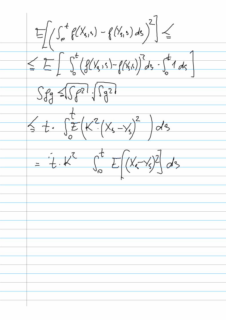
On the other hand, by Cauchy–Schwarz

E

�sups∈[0,t]

(B(n)s )2

�≤ tK2 E

� t

0

�X(n)

s −X(n−1)s

�2ds.

This implies

E

�sups∈[0,t]

(X(n+1)s −X(n)

s )2

�≤ L

� t

0

E(X(n)s −X(n−1)

s )2ds,

with L = 2(T + 4)K2. Iterating and changing the order of integration

E

�sups∈[0,t]

(X(n+1)s −X(n)

s )2

�≤ L

� t

0

E(X(n)s −X(n−1)

s )2 ds

≤ L2

� t

0

� s

0

E(X(n−1)u −X(n−2)

u )2 du ds

≤ L2

� t

0

(t− s)E(X(n−1)s −X(n−2)

s )2 ds.

Continuing, and using the assumption on ξ we obtain

E

�sups∈[0,t]

(X(n+1)s −X(n)

s )2

�

≤ Ln

� t

0

(t− s)n−1

(n− 1)!E(X1

s − ξ)2 ds ≤ C(LT )n

n!.

By Chebyshev

∞�

n=1

P

�sup

0≤t≤T|X(n+1)

t −Xnt | > n−2

�≤

∞�

n=1

C �n4 (LT )n

n!< ∞.

64

Therefore, applying the first Borel–Cantelli lemma the infinite sum∞�

n=0

(X(n+1)t −Xn

t )

converges a.s. Clearly the sum is a solution to the SDE (22).

5.2 Examples

Most of the examples and exercises are from Evans [4].

Example 16. Let g be a continuous function, and consider the SDE�dXt = g(t)XtdWt

X0 = 1.

Show that the unique solution is

Xt = exp

�−1

2

� t

0

g(s)2ds+

� t

0

g(s)dWs

�.

The uniqueness follows from Theorem 32, assuming g is nice enough. Tocheck that Xt is indeed a solution, we use Itô’s formula. Let

Yt = −1

2

� t

0

g(s)2ds+

� t

0

g(s)dWs.

With f(x) = ex, we have

Xt = eYt = 1 +

� t

0

eYsdYs +1

2

� t

0

eYsg2(s)ds

= 1 +

� t

0

Xsg(s)dWs,

as claimed.

Exercise 34. Let f and g be continuous functions, and consider the SDE�dXt = f(t)Xtdt+ g(t)XtdWt

X0 = 1.

Show that the unique solution is

Xt = exp

�� t

0

�f(s)− 1

2g(s)2

�ds+

� t

0

g(s)dWs

�.

65

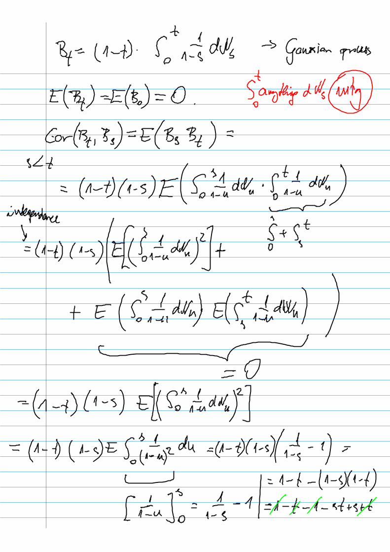
Exercise 35 (Brownian bridge). Show that

Bt = (1− t)

� t

0

1

1− sdWs

is the unique solution of the SDE�dBt = − Bt

1−tdt+ dWt

B0 = 0.

Calculate the mean and covariance function of B.

A mean zero Gaussian process Bt on [0, 1] is called Brownian bridge if itscovariance function is

Cov(Bs, Bt) = min(s, t)− st.

Exercise 36. Show that if W is SBM then Bt = Wt − tW1 is Brownianbridge.

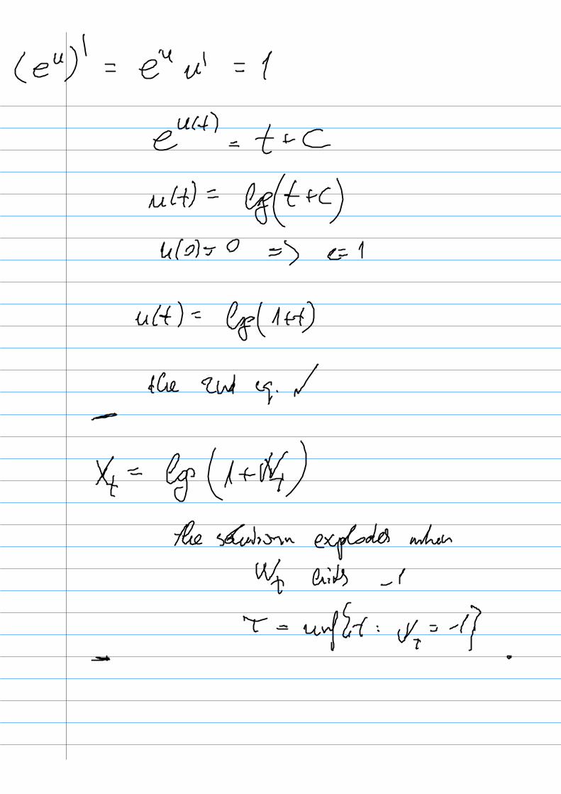
Exercise 37. Solve the SDE�dXt = −1

2e−2Xtdt+ e−XtdWt

X(0) = 0

and show that it explodes in a finite random time. Hint: Look for a solutionXt = u(Wt).

Exercise 38. Solve the SDE

dXt = −Xtdt+ e−tdWt.

Exercise 39. Show that (Xt, Yt) = (cosWt, sinWt) is a solution to the SDE�dXt = −1

2Xtdt− YtdWt

dYt = −12Ytdt+XtdWt.

Show that�

X2t + Y 2

t is a constant for any solution (X, Y )!

66