stochastic geometry and the user experience in a … mukhe… · stochastic geometry and the user...

2011 DOCOMO Innovations, Inc. All Rights Reserved.

Stochastic Geometry and the User Experience in a Wireless Cellular Network

Sayandev Mukherjee DOCOMO Innovations, Inc.

Palo Alto, CA


Future networks will be heterogeneous

2

Spectrum reuse is a popular and effective way to increase capacity within existing spectrum

Existing macro-cells + new small cells = heterogeneous network (HetNet)

Small(er) cells are an effective way to achieve spectrum reuse •  Micro- and Pico-cells: favored

by network operators for offload

•  Femto-cells: offloading and no operator backhaul expense

•  Relays and Remote Radio Heads: applications to enhance coverage and reduce energy consumption

•  Operator-owned D2D transmitters (DII proposal)

The underlying macro network continues to be present and required to meet wide-area coverage requirements

Cisco predic+on: Overall mobile data traffic is expected to grow to 24.3 exa (1018) bytes per month by 2019, nearly a 10x increase over 2014


5/18/15 3

Network densification for greater capacity

1 small (pico) cell per macrocell 30 small (pico) cells per macrocell

Feasible, robust, and relatively cheap: a dense network of small cells overlaid on the existing large-cell (macro-cell) network

Courtesy Prof. Ismail Guvenc, Florida International University, Miami, FL


How to design a ‘good’ HetNet?

4

•  ‘Good’: a chosen set of operational parameters representing a desirable tradeoff between coverage, capacity, and cost

•  Coverage and capacity both depend on the distribution of the Signal to Interference plus Noise ratio (SINR) in the network

•  Thus, before we can design the HetNet, we need to understand the behavior of the SINR in a HetNet

•  Example: considering a picocell overlay on the macrocell network

•  How does the distribution of SINR at an arbitrarily-located user (also called the “typical user”) depend on:

o  The density of picocells relative to macrocells?

o  The transmit power of picocells relative to macrocells?

o  The parameters of the wireless channel model?


New approach: combining insights from analysis with targeted simulations

Exhaustive Simulation •  Study any scenario at any desired

depth of detail

•  Time-consuming to design, code, debug, and run

•  Requires a separate simulation for every scenario and for each choice of parameters of the simulation

•  Number of combinations of deployment parameters rises exponentially in the number of tiers of the HetNet

5

Analysis + Targeted Sim. •  Scales to arbitrary numbers of tiers:

macro/micro/pico/femto-cells, relays, remote radio heads, D2D transmitters

•  Gives overall insights without misinterpreting or being biased by any specific scenario

•  Cannot model detailed aspects of PHY layer design

•  For exact performance results, need simulation

•  Use insights to shrink search space, then run targeted simulations for exact results


5/18/15 6

Definition of SINR at a “typical user”

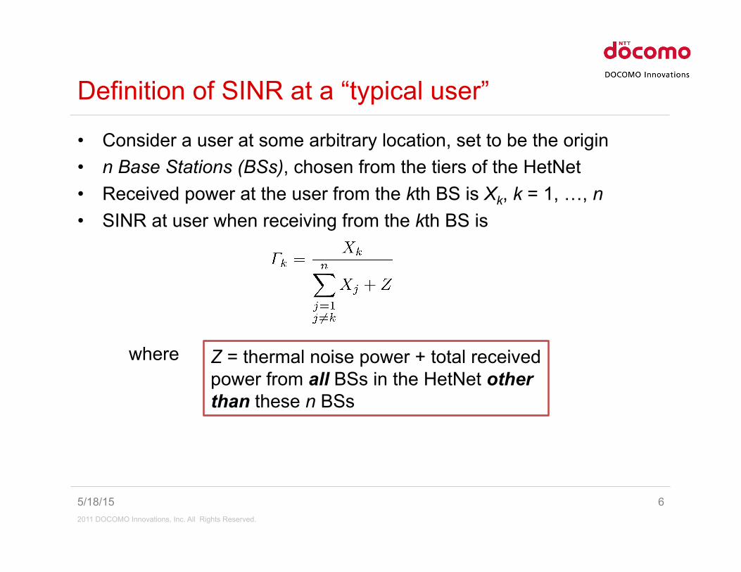
•  Consider a user at some arbitrary location, set to be the origin •  n Base Stations (BSs), chosen from the tiers of the HetNet •  Received power at the user from the kth BS is Xk, k = 1, …, n •  SINR at user when receiving from the kth BS is

where

Z = thermal noise power + total received power from all BSs in the HetNet other than these n BSs


5/18/15 7

Matrix-vector form of important events

•  Recall SINR when receiving from kth BS:

•  The SINR Exceedance Event (used to calculate joint distributions):

•  SINR and Power Exceedance Event: k ≤ n (SINR with tier selection bias):

A X > Z ρ

A X > Z e1


5/18/15 8

Canonical SINR event at “typical user”

•  Take the event that n non-negative random variables X1,…,Xn belong to the region defined by

where A is an n x n real matrix and is an n x 1 vector with all entries nonnegative, and the inequality is interpreted to apply component by component

•  Suppose also that all off-diagonal entries in A are ≤ 0 •  Such a matrix is called a Z-matrix •  We also assume that A is nonsingular •  For future use, we also define an M-matrix as one whose

inverse has all non-negative entries


•  [Berman&Plemmons’94, Thm. 2.3, Chap. 6 (p. 134), Condition (I28)]: The canonical region is entirely in the positive orthant if A is an M-matrix, and entirely outside the positive orthant otherwise –  Further, if A is an M-matrix, then the canonical region is a cone:

5/18/15 9

The structure of the canonical region

A not an M-matrix

0 A is an M-matrix: Cone generated by columns of


5/18/15 10

The probability of the canonical event

•  Suppose that where Z is a random variable that is independent of X1,…,Xn and the latter are independent with Erlang Gamma PDFs for k = 1,…,n:

•  Let

•  Then the probability of the canonical event is (mk = nk-1)


•  Note that to compute we need to be able to tell when a given Z-matrix A is also an M-matrix

•  [Condition (E17),Thm. 2.3, Chap. 6, Berman&Plemmons’94] A is an M-matrix iff every leading principal minor is > 0: det(A([1:k],[1:k])) > 0, k = 1,…,n [Matlab notation]

For the A matrices in our scenarios of interest: •  det(A([1:k],[1:k])) can be computed in closed form •  det(A([1:k],[1:k])) is decreasing in k •  Thus in our scenarios, A is an M-matrix iff det A > 0 •  We will see that we can also calculate A-1 in closed form • Note that = 0 if det A ≤ 0

5/18/15 11

When is a Z-matrix an M-matrix?

A


5/18/15 12

What do we need for analytical modeling?

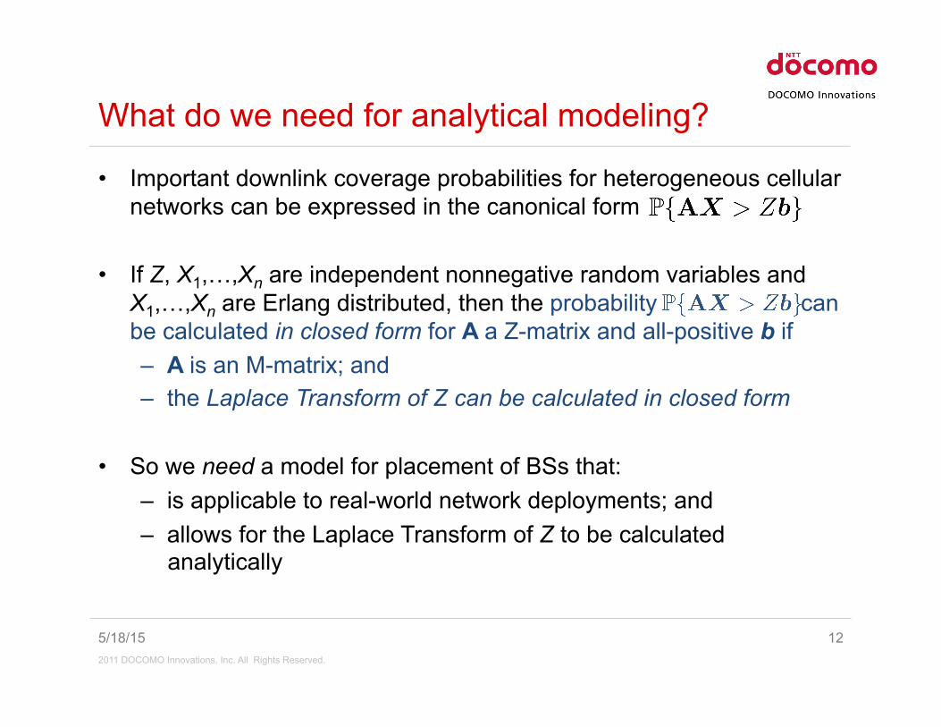
•  Important downlink coverage probabilities for heterogeneous cellular networks can be expressed in the canonical form

•  If Z, X1,…,Xn are independent nonnegative random variables and X1,…,Xn are Erlang distributed, then the probability can be calculated in closed form for A a Z-matrix and all-positive b if –  A is an M-matrix; and –  the Laplace Transform of Z can be calculated in closed form

•  So we need a model for placement of BSs that: –  is applicable to real-world network deployments; and –  allows for the Laplace Transform of Z to be calculated

analytically


5/18/15 13

What about the ideal hexagonal lattice?

•  Dubious applicability to the “real world” •  Cannot compute Laplace Transform of interference analytically •  Same problem for any other finite regular deployment of BSs, but …

From Blaszczyszyn et al., 2010


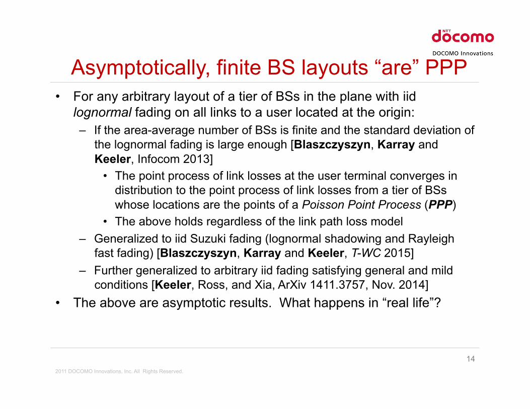
Asymptotically, finite BS layouts “are” PPP •  For any arbitrary layout of a tier of BSs in the plane with iid

lognormal fading on all links to a user located at the origin: –  If the area-average number of BSs is finite and the standard deviation of

the lognormal fading is large enough [Blaszczyszyn, Karray and Keeler, Infocom 2013]

•  The point process of link losses at the user terminal converges in distribution to the point process of link losses from a tier of BSs whose locations are the points of a Poisson Point Process (PPP)

•  The above holds regardless of the link path loss model –  Generalized to iid Suzuki fading (lognormal shadowing and Rayleigh

fast fading) [Blaszczyszyn, Karray and Keeler, T-WC 2015] –  Further generalized to arbitrary iid fading satisfying general and mild

conditions [Keeler, Ross, and Xia, ArXiv 1411.3757, Nov. 2014] •  The above are asymptotic results. What happens in “real life”?

14


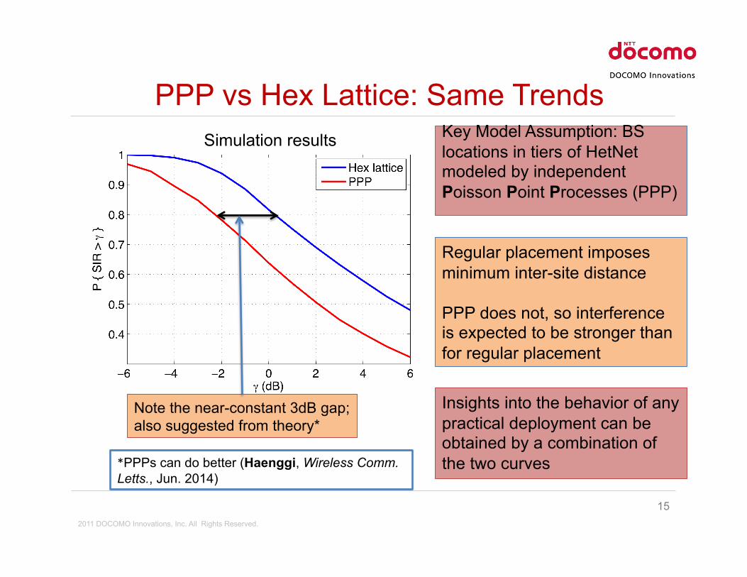
PPP vs Hex Lattice: Same Trends

15

Insights into the behavior of any practical deployment can be obtained by a combination of the two curves

Note the near-constant 3dB gap; also suggested from theory*

Regular placement imposes minimum inter-site distance

PPP does not, so interference is expected to be stronger than for regular placement

Key Model Assumption: BS locations in tiers of HetNet modeled by independent Poisson Point Processes (PPP)

*PPPs can do better (Haenggi, Wireless Comm. Letts., Jun. 2014)

Simulation results


•  Consider a single tier i, say, and a user at the origin •  BSs in this tier are located at points of homogeneous PPP Φi

•  The link loss on the link between BS b ε Φi and this user is

–  Here, αi > 2, the path-loss exponent, is the slope and Ki is the intercept of the slope-intercept path-loss model

–  Rb is the distance between BS b and the user at the origin –  Hb is the fading coefficient on the link (assumed Erlang-Gamma distributed with

unit mean)

•  The received power at the user from BS b ε Φi is

5/18/15 16

Link loss and received power

Fading Coefficient

Transmit power: same across all BSs in a +er

Constant; depends on geometry

Distance of b from user


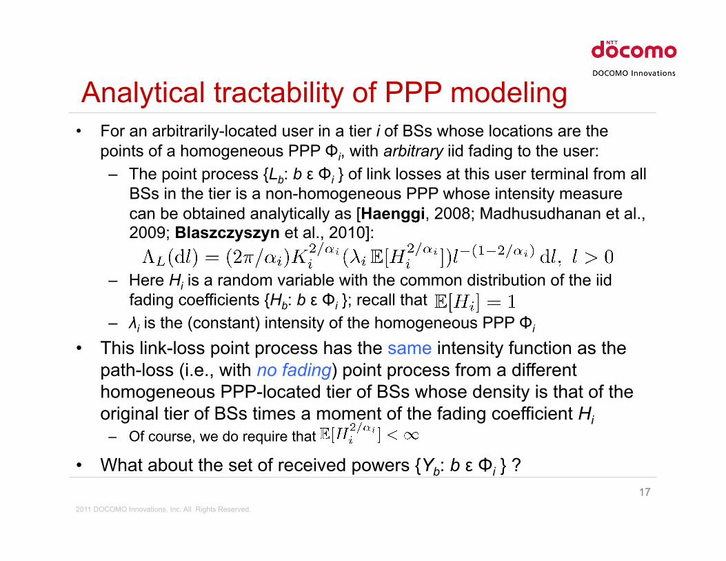
Analytical tractability of PPP modeling •  For an arbitrarily-located user in a tier i of BSs whose locations are the

points of a homogeneous PPP Φi, with arbitrary iid fading to the user: –  The point process {Lb: b ε Φi } of link losses at this user terminal from all

BSs in the tier is a non-homogeneous PPP whose intensity measure can be obtained analytically as [Haenggi, 2008; Madhusudhanan et al., 2009; Blaszczyszyn et al., 2010]:

–  Here Hi is a random variable with the common distribution of the iid fading coefficients {Hb: b ε Φi }; recall that

–  λi is the (constant) intensity of the homogeneous PPP Φi •  This link-loss point process has the same intensity function as the

path-loss (i.e., with no fading) point process from a different homogeneous PPP-located tier of BSs whose density is that of the original tier of BSs times a moment of the fading coefficient Hi

–  Of course, we do require that

•  What about the set of received powers {Yb: b ε Φi } ? 17


Analytical tractability of PPP modeling (contd.) •  Formally applying the Mapping Theorem, the intensity measure of Pi

times the inverse of the link losses is

–  This should be the intensity measure of {Yb: b ε Φi }, but unfortunately, ΛY([0, y]) = ∞ for all y > 0, though ΛY(K) < ∞ for all compact

•  The set {Yb: b ε Φi } of received powers is not a point process on the space [0, ∞) because it has a limit point at 0 –  Fortunately, {0} U [the PPP on (0, ∞) with intensity measure ΛY] is a

Poisson random set [Molchanov, 2005, p. 109] and has the same capacity functional as the PPP on (0, ∞) with intensity measure ΛY

–  Received power is never 0, so we identify {Yb: b ε Φi } with the PPP on (0, ∞) with intensity measure ΛY (dy) = (C/y1+δ ) dy

–  Consequence: The signal to signal-plus-interference ratio, called signal to total interference ratio or STIR, is a two-parameter Poisson-Dirichlet point process [Keeler and Blaszczyszyn, Wireless Comm. Letts., Oct. 2014]

18


Cell association in a cellular network •  In LTE, all BSs transmit reference symbols (RSs) that identify them •  A user terminal aggregates multiple measurements of the received

reference symbol signals and smooths out fast fading •  Serving BS(s) are selected on the basis of the smoothed reference

symbol STIR, called reference symbol received quality or RSRQ) •  Assume residual fading is slow only, iid across all links to the user •  Then, for RSRQ distribution, the BS deployment is equivalent to

another homogeneous PPP without fading and an adjusted density –  In each tier, the n “strongest” BSs (original deployment) ! the n nearest BSs –  For coordinated multipoint (CoMP) transmissions from BSs in a given tier i, we

select the n “strongest” BSs (original deployment) where the nth-strongest is no more than, say, τi dB weaker in RSRQ than the strongest ! conditions on the distances of the n nearest BSs

–  For selection of serving BS(s) across tiers of a HetNet, the RSRQs from the candidate serving BS(s) in each tier i are weighted by tier selection bias factors, then compared across all tiers

19


Coverage in a cellular network •  Consider an arbitrarily-located user (a “typical user”) in a cellular

network (possibly with multiple tiers) •  The coverage probability for this user is the probability that the

RSRQ (from its set of serving BS(s) selected across all tiers) exceeds some threshold (which may be dependent upon the tiers of the serving BSs)

–  The joint distribution of the top n ordered RSRQs from each tier is available analytically from the fact that the STIRs form a two-parameter Poisson-Dirichlet point process [Handa, Bernoulli vol. 15, no. 4, pp. 1082-1116, 2009]

•  Note that coverage is defined in terms of received STIR of the reference symbols, not data symbols

•  In other words, coverage just means that the user can maintain radio contact with the selected serving BS(s), but says nothing about the bit rate of data traffic on such links

20


Instantaneous (data) SINR in a cellular network •  Consider an arbitrarily-located user (a “typical user”) in a cellular

network (possibly with multiple tiers) •  The data SINR is the instantaneous SINR at this user when it is

receiving data (not reference symbols) from the serving BS(s) selected on the basis of (smoothed) RSRQ

–  Note that candidate serving BSs from each tier were selected on the basis of geometric proximity to the user (in the equivalent network with no fading)

–  However, even in this equivalent network, when the selected serving BS(s) transmit data to the user, the instantaneous SINR now includes the fast fading on the links between these BSs and the user

•  Example: Candidate serving BS in each tier is the (single) nearest BS (to the user) in that tier; n tiers; the single serving BS is the instantaneous strongest one (without tier selection bias); instantaneous SINR distribution is

21

SINR Exceedance Event


5/18/15 22

Recall

•  The SINR exceedance event can be expressed as •  If Z, X1,…,Xn are independent nonnegative random variables and

X1,…,Xn are Erlang distributed, then the probability can be calculated in closed form for A a Z-matrix and all-positive b if –  A is an M-matrix; and –  the Laplace Transform of Z can be calculated in closed form

•  We shall see that: –  The corresponding Laplace Transform for Z can be calculated in closed

form when base station locations are modeled by PPPs but not when they are placed on a regular hexagonal lattice, say

–  Compared to regular hexagonal lattice located BS placement, interference power is always higher for PPP placement

•  Reason: no minimum distance requirement between BSs in PPP model

•  Thus, PPP model yields conservative results for coverage


•  Consider a single tier i, say •  BSs in this tier are located at points of homogeneous PPP Φi •  Received power at user from BS b ε Φi is

•  Want Laplace Transform of total received power at user from all BSs

in tier i that are at least at distance d from the user:

5/18/15 23

Single tier: Laplace Transform of Z

Probability Genera+ng Func+onal


•  Assume i.i.d. Rayleigh fading on all links, no noise, all n tiers open •  Assume candidate serving BSs for the user are the nearest BSs in

the n tiers, whose distances rk from the user are known •  Conditioned on these distances, the received power Xk at user from

the candidate serving BS in tier k is Exponential with mean 1/ck

•  Let the SIR at the user if it is served by the kth candidate serving BS be Γk . Then the joint distribution of these SIRs given {rk} is

5/18/15 24

Example 1: joint distribution of SIR from tiers


•  Single-tier, no noise, serving BS is nearest one to user at distance r1 •  Conditioned on this distance, the received power X1 at user from the

serving BS is Erlang-Gamma:

•  From the expressions for the probability of the canonical event, the distribution of SIR is given by

where

•  [Li, Zhang, and Ben Letaief, T-WC May 2014] show that

where T = [Tij]i,j=0,…,m is a certain lower-triangular Toeplitz matrix 5/18/15 25

Example 2: single tier, X1 Erlang-Gamma


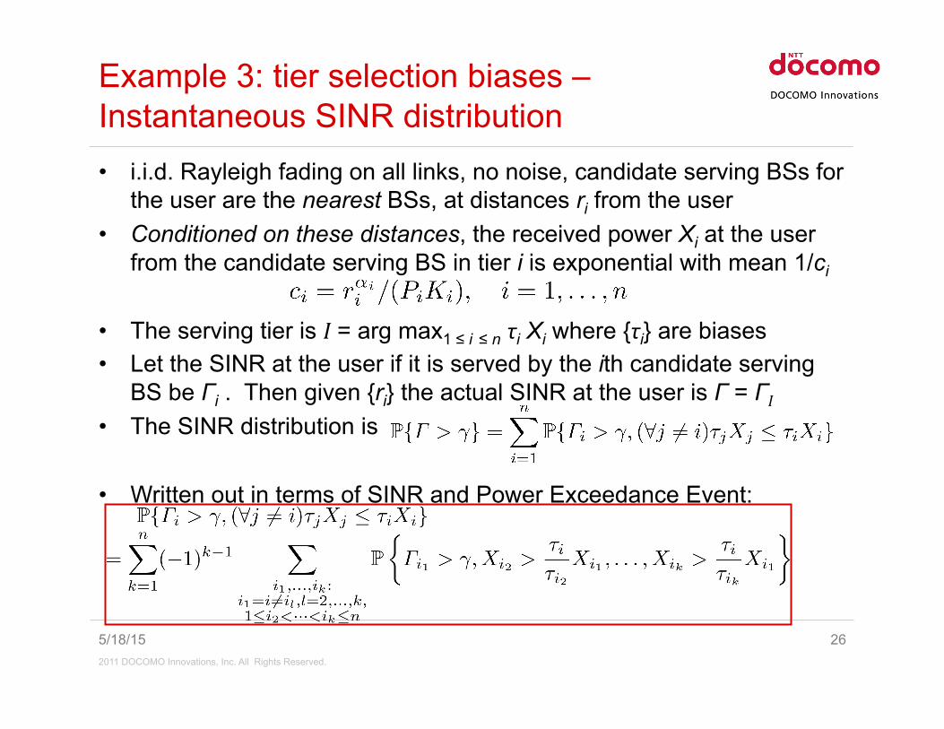
•  i.i.d. Rayleigh fading on all links, no noise, candidate serving BSs for the user are the nearest BSs, at distances ri from the user

•  Conditioned on these distances, the received power Xi at the user from the candidate serving BS in tier i is exponential with mean 1/ci

•  The serving tier is I = arg max1 ≤ i ≤ n τi Xi where {τi} are biases •  Let the SINR at the user if it is served by the ith candidate serving

BS be Γi . Then given {ri} the actual SINR at the user is Γ = ΓI •  The SINR distribution is

•  Written out in terms of SINR and Power Exceedance Event:

5/18/15 26

Example 3: tier selection biases – Instantaneous SINR distribution


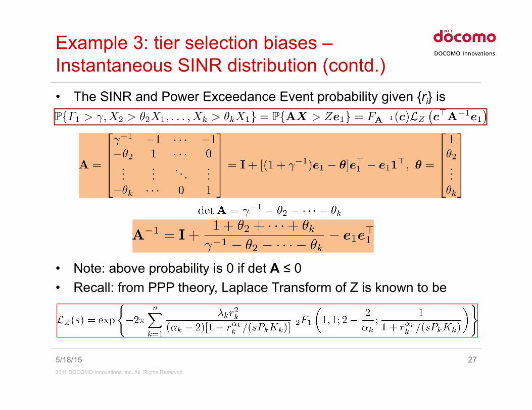
•  The SINR and Power Exceedance Event probability given {ri} is

•  Note: above probability is 0 if det A ≤ 0 •  Recall: from PPP theory, Laplace Transform of Z is known to be

5/18/15 27

Example 3: tier selection biases – Instantaneous SINR distribution (contd.)


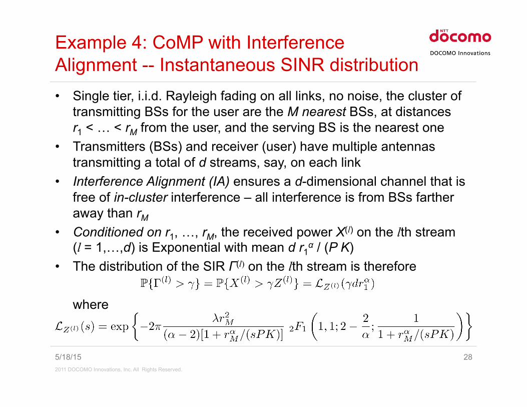
•  Single tier, i.i.d. Rayleigh fading on all links, no noise, the cluster of transmitting BSs for the user are the M nearest BSs, at distances r1 < … < rM from the user, and the serving BS is the nearest one

•  Transmitters (BSs) and receiver (user) have multiple antennas transmitting a total of d streams, say, on each link

•  Interference Alignment (IA) ensures a d-dimensional channel that is free of in-cluster interference – all interference is from BSs farther away than rM

•  Conditioned on r1, …, rM, the received power X(l) on the lth stream (l = 1,…,d) is Exponential with mean d r1

α / (P K) •  The distribution of the SIR Γ(l) on the lth stream is therefore

where

5/18/15 28

Example 4: CoMP with Interference Alignment -- Instantaneous SINR distribution


•  Now let the user be served by the BS that is received with maximum power at that instant (i.e., with maximum instantaneous SIR)

•  For a single-tier deployment, the relationship between STIR and the two-parameter Poisson-Dirichlet process yields the PDF of the maximum STIR (and therefore also the maximum SIR)

•  For more than one tier, let Φ be the superposition PPP over all tiers. When receiving from any BS b in Φ, if the received power at the useris Yb, the SINR is

•  The distribution of maximum instantaneous SIR is thus

5/18/15 29

Example 5: Instantaneous switching – maximum instantaneous SIR distribution


•  For each tier Φk, the iid fades may be assumed Rayleigh after appropriately adjusting the density of the BS PPP for that tier

•  Then the set of received powers Ψk = {Yb: b ε Φk } is identified with the non-homogeneous 1-D PPP with intensity function

•  Then over all sets of q = n1 + … + nm BSs we have

5/18/15 30

Example 5 (contd.): Computing the terms Slivnyak-‐M

ecke The

orem


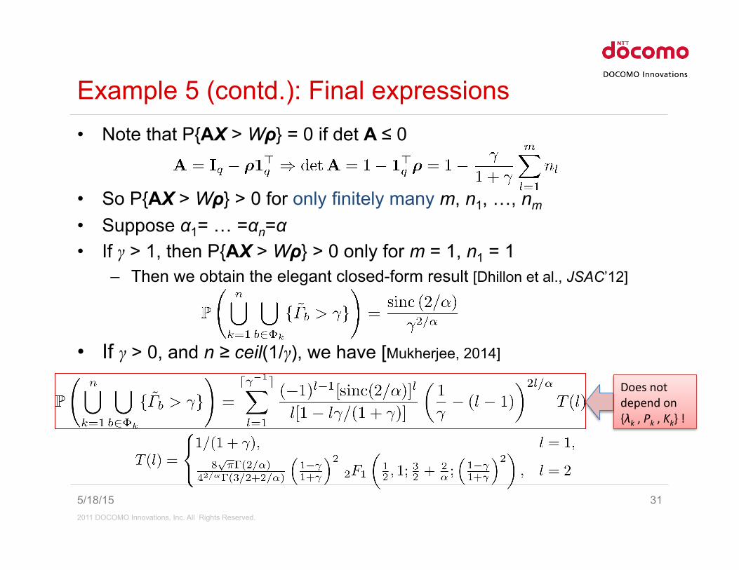
•  Note that P{AX > Wρ} = 0 if det A ≤ 0

•  So P{AX > Wρ} > 0 for only finitely many m, n1, …, nm •  Suppose α1= … =αn=α •  If γ > 1, then P{AX > Wρ} > 0 only for m = 1, n1 = 1

–  Then we obtain the elegant closed-form result [Dhillon et al., JSAC’12]

•  If γ > 0, and n ≥ ceil(1/γ), we have [Mukherjee, 2014]

5/18/15 31

Example 5 (contd.): Final expressions

Does not depend on {λk , Pk , Kk} !


•  The serving BS is the one that is received with maximum RSRQ at the user (i.e., with maximum STIR, equivalent to maximum SIR)

•  Let Φ be the PPP of all BS locations. When receiving from any BS b in Φ, if the received power at the user is Yb, the SIR is

•  Suppose the SIR threshold for coverage by tier k is βk •  The probability of coverage is thus

5/18/15 32

Example 6: coverage probability in a multi-tier HetNet


•  Note that P{AX > Wρ} = 0 if det A ≤ 0

•  So P{AX > Wρ} > 0 for only finitely many m, n1, …, nm •  Suppose α1= … =αn=α •  If β1,…, βn > 1, then P{AX > Wρ} > 0 only for m = 1, n1 = 1

–  Then [Dhillon et al., JSAC’12]

= Probability that a randomly-selected BS belongs to tier k in an equivalent overall network with density and P = 1, K = 1 for all BSs

5/18/15 33

Example 6 (contd.): coverage probability


5/18/15 34

What about non-Erlang distributed Xk ? •  [DeVore&Lorentz’93, Problem 5.6, p. 14] An arbitrary PDF can be uniformly

approximated by an infinite mixture of Erlang Gamma densities:

•  X1,…,Xn are the received powers over wireless links –  For Nakagami fast fading with lognormal slow fading, finite Gamma

(but not necessarily Erlang) mixture approximations to the PDF of Xk have been provided in [Atapattu et al., T-WC’11]

–  Convert to finite Erlang Gamma mixture using the method in eqns. (16)-(17) of [Almhana et al., ICC’06]


Data rates in a cellular network •  Conditioned on the distances to the BSs and the fades on the links

from those BSs to the user, the achievable data rate to the user is given by Shannon’s formula: C = log2(1 + Γ) bits/s/Hz

•  Here Γ is is the instantaneous data rate to the user •  The mean achievable data rate to the user is therefore

•  This is a measure of the Service Quality as experienced by the user –  User is interested only in his/her own data rate, not that of others –  The above is the expected achievable data rate for a “typical user” –  Says nothing about the service quality experienced by many

simultaneous users of the network, which is what the network operator is interested in

–  Need to define the appropriate metric from the network operator’s PoV 35


Data rates in a cellular network (contd.) •  The network operator is interested in the mean achievable total

throughput to all users served in a typical cell (bits/s/Hz) •  Single-tier PPP with density λ: mean area of the typical cell = 1/λ •  Average throughput per unit area = λ x the mean achievable total

throughput to all users served in a typical cell (bits/s/Hz/km2) •  Recall: users are served by nearest BSs in an equivalent PPP •  So: typical cell is that in the Poisson-Voronoi tessellation

–  Where are the users in this typical cell? –  How does the BS decide which of these users to serve at a given instant?

•  Simplify: assume user locations given by independent PPP, so –  User locations are iid uniformly distributed over the typical cell –  BS simply cycles through these users serving one at a time (round-robin)

•  Total throughput to users in typical cell = throughput to a single user whose location is uniformly distributed over the typical cell

•  Distribution of distance between user and nucleus of typical cell? 36


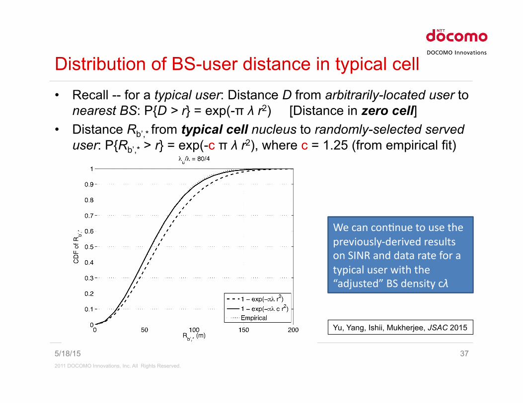
•  Recall -- for a typical user: Distance D from arbitrarily-located user to nearest BS: P{D > r} = exp(-π λ r2) [Distance in zero cell]

•  Distance Rb’,* from typical cell nucleus to randomly-selected served user: P{Rb’,* > r} = exp(-c π λ r2), where c = 1.25 (from empirical fit)

5/18/15 37

Distribution of BS-user distance in typical cell

We can con+nue to use the previously-‐derived results on SINR and data rate for a typical user with the “adjusted” BS density cλ

Yu, Yang, Ishii, Mukherjee, JSAC 2015


5/18/15 38

Is E[log2(1 + Γ)] the ergodic rate to a user? •  No, because Γ is the instantaneous SINR (for a system snapshot) •  The ergodic rate by definition requires transmissions to be long

enough to encounter every state of the channel •  For ergodic rate: average over all states of the channel to the user --

–  Consider single tier, homogeneous PPP located BSs –  BSs transmit iid complex symbols –  Baseband equivalent complex total interference signal at any user

location from all BSs more than some distance away is not Gaussian [Gulati et al., T-SP 2010, Guan and Di Renzo, T-COM 2014]

–  Verified by simulation [Aljuaid and Yanikomeroglu, T-VT 2010]

•  However, using a codebook and decoder designed for Gaussian noise, the spectral efficiency is as if the interference were Gaussian! [Lapidoth and Shamai, T-IT 2002]

•  Then use E [log2(1 + SIR)] for ergodic rate by approximating interference by CAWGN with the same covariance matrix [Mungara et al., 2015]


5/18/15 39

Conclusions •  Number and variety of deployment scenarios for HetNets too great

for detailed simulation study of each and every one of them •  PPP location model for BSs in the tiers of a HetNet

–  Is mathematically tractable and scalable to arbitrary numbers of tiers –  Yields important insights into SINR distributions throughout the network,

e.g., coverage in a single-tier network is not dependent on BS density –  For important special cases of practical interest, closed-form results are

obtainable for coverage –  Compared to the ‘classical’ regular hexagonal BS location model, the

PPP model yields conservative results for both coverage probability and ergodic rate to arbitrarily-located users

•  The zero-cell versus typical-cell calculations illustrate the quality of the experience from the perspectives of the user and the network operator, respectively

•  Substantial additional approximate results available by relaxing certain assumptions


5/18/15 40

References •  A. Berman, R.J. Plemmons, Nonnegative matrices in the mathematical sciences, SIAM Classics in

Appl. Math., 1994 •  B. Błaszczyszyn, M.K. Karray, F.X. Klepper, “Impact of the geometry, path-loss exponent and random

shadowing on the mean interference factor in wireless cellular networks,” Proc. WMNC 2010 •  B. Błaszczyszyn, M.K. Karray, H.P. Keeler, “Using Poisson processes to model lattice cellular networks,”

Proc. IEEE INFOCOM 2013 •  B. Błaszczyszyn, M.K. Karray, H.P. Keeler, “Wireless Networks appear Poissonian due to strong

shadowing,” IEEE Trans. Wireless Comm., 2015 •  H.P. Keeler, N. Ross, A. Xia, “When do wireless network signals appear Poissonian?” ArXiv 1411.3757,

Nov. 2014 •  M. Haenggi, “The Mean Interference-to-Signal Ratio and its Key Role in Cellular and Amorphous

Networks,” IEEE Wireless Comm. Letts., 3(6):597--600, 2014 •  M. Haenggi, “A geometric interpretation of fading in wireless networks: theory and applications,” IEEE

Trans. Inform. Theory 54(12):5500–5510, 2008. •  P. Madhusudhanan, J.G. Restrepo, Y. Liu, T.X. Brown, “Carrier to Interference Ratio Analysis for the

Shotgun Cellular System,” Proc. IEEE Globecom 2009 •  I. Molchanov, Theory of Random Sets, Springer, 2005 •  P. Keeler, B. Błaszczyszyn, “SINR in Wireless Networks and the Two-Parameter Poisson-Dirichlet

Process,” IEEE Wireless Comm. Letts., 3(5):525—528, Oct. 2014 •  K. Handa, “The Two-Parameter Poisson-Dirichlet Point Process,” Bernoulli 15(4):1082-1116, 2009 •  C. Li, J. Zhang, K.B. Letaief, “Throughput and Energy Efficiency Analysis of Small Cell Networks with

Multi-Antenna Base Stations,” IEEE Trans. Wireless Comm., 13(5):2505—2517, May 2014


5/18/15 41

References (contd.) •  H.S. Dhillon, R.K. Ganti, F. Baccelli, J.G. Andrews, “Modeling and Analysis of K-Tier Downlink

Heterogeneous Cellular Networks,” IEEE JSAC 30(3):550-560, Apr. 2012 •  S. Mukherjee, Analytical Modeling of Heterogeneous Cellular Networks, Cambridge, 2014 •  R.A. DeVore, G.G. Lorentz, Constructive Approximation, Springer, 1993 •  S. Atapattu, C. Tellambura, H. Jiang, “A Mixture Gamma Distribution to Model the SNR of Wireless

Channels,” IEEE Trans. Wireless Comm., 10(12):4193-4203, Dec. 2011 •  J. Almhana, Z. Liu, V. Choulakian, R. McGorman, “A Recursive Algorithm for Gamma Mixture Models,”

Proc. IEEE ICC 2006, pp. 197-202 •  B. Yu, L. Yang, H. Ishii, S. Mukherjee, “Dynamic TDD Support in Macrocell-Assisted Small Cell

Architecture,” IEEE JSAC 33(6):1201—1213, 2015 •  K. Gulati, B.L. Evans, J.G. Andrews, K.R. Tinsley, “Statistics of Co-Channel Interference in a Field of

Poisson and Poisson-Poisson Clustered Interferers,” IEEE Trans. Sig. Proc., 58(12):6207-6222, 2010 •  M. Aljuaid, H. Yanikomeroglu, “Investigating the Gaussian Convergence of the Distribution of the

Aggregate Interference Power in Large Wireless Networks,” IEEE Trans. Veh. Tech., 59(9):4418-4424, Nov. 2010

•  P. Guan, M. Di Renzo, “A Mathematical Framework to the Computation of the Error Probability of Downlink MIMO Cellular Networks by Using Stochastic Geometry”, IEEE Trans. Communications, 62(8):2860-2879, Aug. 2014

•  A. Lapidoth and S. Shamai, “Fading channels: how perfect need ‘side information’ be?” IEEE Trans. Inform. Theory, 48(5):1118-1134, May 2002

•  R. Mungara, D. Morales-Jimenez, A. Lozano, “System-level Performance of Interference Alignment,” IEEE Trans. Wireless Commun., 14(2):1060-1070, Feb. 2015

stochastic geometry and the user experience in a … mukhe… · stochastic geometry and the user...

Documents