centre for stochastic geometry and advanced bioimaging...

CENTRE FOR STOCHASTIC GEOMETRYAND ADVANCED BIOIMAGING

RESEARCH REPORTwww.csgb.dk

2011Kristjana Yr Jonsdottir, Anders Rønn-Nielsen, Kim Mouridsenand Eva B. Vedel Jensen

Lévy Based Modelling in Brain Imaging

No. 02, April 2011

Lévy Based Modelling in Brain Imaging

Kristjana Yr Jonsdottir1,2, Anders Rønn-Nielsen3, Kim Mouridsen1

and Eva B. Vedel Jensen2,4

1Center of Functionally Integrative Neuroscience, Aarhus University2Department of Mathematical Sciences, Aarhus University

3Department of Mathematical Sciences, University of Copenhagen4Centre for Stochastic Geometry and Advanced Bioimaging, Aarhus University

Abstract

Traditional methods of analysis in brain imaging based on Gaussian randomfield theory may leave small, but significant changes in the signal level unde-tected, because the assumption of Gaussianity is not fulfilled. In group compar-isons, the number of subjects in each group is usually small so the alternativestrategy of using a non-parametric test may not be appropriate either becauseof low power. We propose to use a flexible, yet tractable model for a randomfield, based on kernel smoothing of a so-called Lévy basis. The resulting fieldmay be Gaussian but there are many other possibilities, e.g. random fieldsbased on Gamma, inverse Gaussian and normal inverse Gaussian (NIG) Lévybases. We show that it is easy to estimate the parameters of the model andaccordingly to assess by simulation the quantiles of a test statistic. A findingof independent interest is the explicit form of the kernel function that inducesa covariance function belonging to the Matérn family.

Keywords: Covariance, cumulant, Gaussian random field, Matérn covariancefunction, non-Gaussian random field, normal inverse Gaussian Lévy basis

1 Introduction

Neuroimaging studies typically aim to detect localized changes in brain structure,physiology, or neuronal activity attributable to disease and/or therapeutic interven-tion. Positron emission tomography (PET) is the current gold standard for imagingkey physiological markers such as cerebral blood flow and blood volume, but suchmeasures can also be obtained without the use of radioactive tracers using MRI.Additionally MRI can produce high resolution images of brain anatomy. Further,MRI is used intensively in the study of human brain function (fMRI) where serialimages are acquired while subjects perform specific mental tasks.

To enable detection of regional changes, the measure of interest is recorded ineach volume element (voxel) of the brain. In group comparisons, such a field of

Corresponding author: Kristjana Yr Jonsdottir, [email protected]

1

measurements is obtained for each subject belonging to a disease/treatment groupand a control group. Typically, a t−test of the hypothesis of no difference between thetwo groups is performed at each voxel, resulting in a field of thousands of correlatedt−statistics.

To control the false positive rate, various methods to evaluate the field of teststatistics have been proposed. A very useful review of these methods can be foundin Nichols and Hayasaka (2003). Apart from the Bonferroni procedure that usuallydisregards the dependence of the test statistics, methods based on random fieldtheory (Worsley 1994, Worsley et al. 1992, Worsley et al. 1996) are very popular.Under the assumption that the random field is Gaussian or Gaussian derived, theP−value of the maximum of the field can be approximated by the expected Eulercharacteristic of the excursion set. An alternative to the maximum is to considerunder a Gaussian assumption the size of the largest connected component of theexcursion set (Cao 1999). It is, however, wellknown that the Gaussian assumptionof the random field may be too restrictive, cf. Salmond et al. (2002), Viviani et al.(2007) and references therein. Furthermore, it has been shown that the geometryof excursion sets is considerably more complicated for non-Gaussian random fieldsthan for Gaussian random fields (Adler et al. 2010a,b).

Unfortunately, there are at the moment no methods of evaluating the robustnessof this analysis against the departures from Gaussianity seen in a concrete dataset. In group comparisons, an alternative is to use a permutation test (Nichols andHolmes 2001) but this test may have low power in the cases where the number ofsubjects in each group is small, as is typical. This is exactly the situation wheredepartures from Gaussianity may affect most severely the null distribution of thefield of test statistics.

The present paper takes up this problem. We propose a flexible, yet tractablemodel for a random field, based on kernel smoothing of a Lévy basis, an indepen-dently scattered, infinitely divisible random measure. (The short terminology of aLévy basis has been introduced in Barndorff-Nielsen and Schmiegel (2004), see alsoWolpert (2001)). This type of model has earlier been used with success in modellingof turbulence (Barndorff-Nielsen and Schmiegel 2004), Cox point processes (Hell-mund et al. 2008) and growth (Jónsdóttir et al. 2008). We derive the kernel functionthat induces the flexible Matérn covariance function (Guttorp and Gneiting 2006).Earlier, specific covariance functions such as the exponential and Gaussian covari-ance functions have been considered in Bowman (2007) and Spence et al. (2007).The Lévy basis may be Gaussian but there are many other possibilities, e.g. Gamma,inverse Gaussian and normal inverse Gaussian to name a few. We show that it iseasy to estimate the parameters of the model and accordingly to assess by simulationthe quantiles of the distribution of the maximum of the field of test statistics.

Furthermore, we expect that the proposed extended random field model will haveindependent interest in functional neuroimaging. Gaussian random fields only focuson the mean, variance and covariance. Interesting changes due to disease or therapythat imply that the distribution of the measurement has more heavy tails or is moreskewed can only be modelled if one goes beyond Gaussianity.

The present paper is organized as follows. In Section 2, we give a short introduc-tion to Gaussian random fields and the notation used for covariances and cumulants,

2

while Section 3 gives a number of examples of kernel functions and their inducedcovariance functions. In particular, the kernel function, inducing a covariance func-tion belonging to the Matérn family, is given in Section 3. In Section 4, we give anexample of brain imaging data that cannot be described satisfactory by a Gaussianrandom field. This motivates us to consider Lévy based random fields and their sta-tistical inference in Sections 5 and 6. The data set is reanalyzed, using a model basedon the normal inverse Gaussian distribution in Section 7 and consequences for brainimaging are discussed in Section 8. Our findings are put into further perspective inSection 9. The derivation of the kernel function that induces the Matérn covariancefunction is deferred to the Appendix.

2 Gaussian random fields, covariances andcumulants

Let xv be the observation at the site (pixel or voxel) with coordinate v ∈ V , whereV is a bounded subset of Rd, d = 2 or 3.

In case V ⊆ Zd, a simple example of a Gaussian random field is given by thefollowing equation

Xv =∑

u∈Zd

k(v, u)Zu, (2.1)

where k is a kernel function and the Zus are independent and identically distributedGaussian random variables. This type of model is very similar to moving averagemodels for time series (Gaetan and Guyon 2010, Section 1.7.1, Wolpert 2001).

Let Z be a random variable with the common distribution of the Zus. Under themodel (2.1), the covariances take the form

Cov(Xv1 , Xv2) = Var(Z)∑

u∈Zd

k(v1, u)k(v2, u), (2.2)

while the cumulants of the random variables Xv can be expressed as

κn(Xv) = κn(Z)∑

u∈Zd

k(v, u)n, n = 1, 2, . . . , (2.3)

since the Xvs are linear combinations of independent random variables.The model (2.1) may be formulated continuously as

Xv =

∫

Rd

k(v, u)Z( du), (2.4)

where Z is an independently scattered, stationary Gaussian random measure (Gae-tan and Guyon 2010, Section 1.5.1). It turns out that under mild regularity condi-tions any Gaussian random field can be described in this fashion, cf. e.g. Hellmundet al. (2008, Proposition 6).

Suppose thatZ( du) ∼ N(µ du, τ 2 du),

3

and let Z ′ ∼ N(µ, τ 2). Then, under the continuous formulation (2.4), (2.2) takes theform

Cov(Xv1 , Xv2) = Var(Z ′)

∫

Rd

k(v1, u)k(v2, u) du. (2.5)

Furthermore, (2.3) becomes

κn(Xv) = κn(Z ′)

∫

Rd

k(v, u)n du, n = 1, 2, . . . . (2.6)

Covariances and cumulants of Xv can thus directly be expressed in terms of thecumulants of Z ′, if the relevant integrals of the kernel function can be calculatedexplicitly.

In the remaining part of the paper, we will assume that k(u, v) = k(u− v), say,and that ∫

Rd

k(u) du = 1.

If we letK(v) =

∫

Rd

k(u)k(v + u) du,

thenCov(Xv1 , Xv2) = Var(Z ′)K(v1 − v2).

If K(v) = K(‖v‖), say, the covariance

Cov(Xv1 , Xv2) = C(‖v1 − v2‖) = Var(Z ′)K(‖v1 − v2‖)

depends only on the distance between sites. The correlation function takes the form

ρ(h) = K(h)/K(0), h ≥ 0.

The variogram γ, defined as E(Xv1 − Xv2)2, depends in this case also only on the

distance between sites and can be expressed as

γ(h) = 2 Var(Z ′)(K(0)−K(h)).

A normalized version of the variogram is

γ̄(h) = γ(h)/Var(Xv) = 2(1− ρ(h)).

3 Covariance models

In this section, we give examples of kernel functions k and induced covariance struc-tures determined by K. For further details, see Cressie (1993) and Gaetan andGuyon (2010, Section 1.5.1). We also give the explicit form of

∫Rd k(v, u)n du for the

different kernels when possible. The kernel function that induces the general Matérncovariance model, see Example 3 below, is to the best of our knowledge not availablein the literature.

4

Example 1 (Spherical covariance). Suppose that

k(u, v) = 1[‖u− v‖ ≤ R]/|B(0, R)|.

Then, if ω ∈ Sd−1 is a unit vector in Rd,

K(h) =|B(0, R) ∩B(hω,R)|

|B(0, R)|2

and ∫

Rd

k(v, u)n du = |B(0, R)|−n+1.

For d = 3, we get

K(h) =1

|B(0, R)|

(1 +

h

4R

)(1− h

2R

)2

1[h ≤ 2R].

Example 2 (Gaussian covariance). Suppose that

k(u, v) =1

(2πσ2)d/2exp

(− 1

2σ2‖u− v‖2

).

Then,

K(h) =1

(4πσ2)d/2exp

(− 1

4σ2h2)

and ∫

R3

k(v, u)n du = n−d/2(2πσ2)−d(n−1)/2.

Example 3 (Matérn covariance). In the Appendix, we derive the kernel functionthat induces a covariance function belonging to the Matérn family, see Guttorp andGneiting (2006) and references therein. It is shown that if

k(u, v) =λd

πd/22ν/2−1+3d/4Γ(ν+d/2

2

)‖λ(u− v)‖ν/2−d/4Kν/2−d/4(λ‖u− v‖), (3.1)

then

K(h) =λd

πd/22d+ν−1Γ(ν + d/2)(λh)νKν(λh). (3.2)

Here, Kν is the modified Bessel function of the second kind, and λ and ν are positiveparameters.

As shown in the supplement file, the flexible Matérn covariance family includesa number of well-known covariance functions. Let us concentrate on the 3D case,i.e. d = 3. For d = 3 and ν = 1

2, (3.1) becomes

k(u, v) =λ2

4π‖u− v‖ exp (−λ‖u− v‖) ,

5

and (3.2) is the exponential covariance function

K(h) =λ3

8πexp (−λh) .

For d = 3 and ν = 52, the kernel function (3.1) is of the form

k(u, v) =λ3

8πexp (−λ‖u− v‖) ,

and (3.2) is the 3rd order autoregressive covariance function

K(h) =λ3

64πexp (−λh)

(λ2

3h2 + λh+ 1

).

In order to evaluate the cumulant relation (2.6), we will also need to evaluate∫Rd k(v, u)n du. For n = 2, we get, see the Appendix,

∫

Rd

k(v, u)2 du =λdΓ(ν)

2dπd/2Γ(ν + d/2). (3.3)

For n > 2, it can be shown that∫

Rd

k(v, u)n du <∞ for ν > ν(d, n),

where the limit ν(d, n) depends on n and d: ν(2, 3) = 13, ν(2, 4) = 1

2, ν(3, 3) = 1

2and

ν(3, 4) = 34. In particular, for the exponential covariance model in R3 (d = 3, ν = 1

2),

we get ∫

R3

k(v, u)n du =∞, n > 2,

Analytic forms of the integrals∫Rd k(v, u)n du can be derived for some parameter

values, in other cases the integrals have to be evaluated numerically. For the 3rdorder autoregressive model in R3 (d = 3, ν = 5

2), we have

∫

R3

k(v, u)n du =1

n3

(λ3

8π

)n−1, n ≥ 2. (3.4)

Note that the last equation also holds for n = 2. Further details are provided in theAppendix.

4 Data example

We obtained dynamic susceptibility contrast magnetic resonance imaging (MRI)scans from four healthy subjects (1.5Tesla, gradient echo, TR/TE = 1500ms/30ms).From these scans, maps of vascular mean transit time (MTT), were calculated usingsingular value decomposition (Wu et al. 2003; Østergaard et al. 1996). The MTTmeasurements are recognized as a valuable indicator of the cerebral blood circulation(Helenius et al. 2003; Ibaraki et al. 2007; Ito et al. 2003). While MTT is at a stable

6

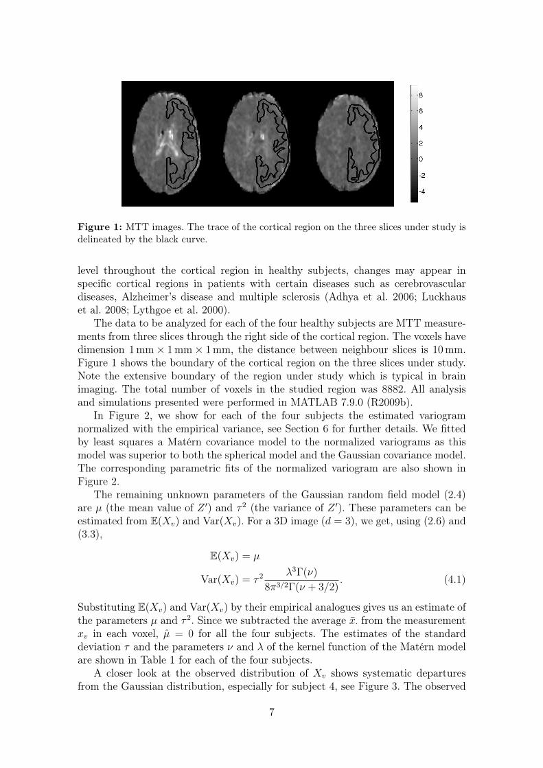
Figure 1: MTT images. The trace of the cortical region on the three slices under study isdelineated by the black curve.

level throughout the cortical region in healthy subjects, changes may appear inspecific cortical regions in patients with certain diseases such as cerebrovasculardiseases, Alzheimer’s disease and multiple sclerosis (Adhya et al. 2006; Luckhauset al. 2008; Lythgoe et al. 2000).

The data to be analyzed for each of the four healthy subjects are MTT measure-ments from three slices through the right side of the cortical region. The voxels havedimension 1mm× 1mm× 1mm, the distance between neighbour slices is 10mm.Figure 1 shows the boundary of the cortical region on the three slices under study.Note the extensive boundary of the region under study which is typical in brainimaging. The total number of voxels in the studied region was 8882. All analysisand simulations presented were performed in MATLAB 7.9.0 (R2009b).

In Figure 2, we show for each of the four subjects the estimated variogramnormalized with the empirical variance, see Section 6 for further details. We fittedby least squares a Matérn covariance model to the normalized variograms as thismodel was superior to both the spherical model and the Gaussian covariance model.The corresponding parametric fits of the normalized variogram are also shown inFigure 2.

The remaining unknown parameters of the Gaussian random field model (2.4)are µ (the mean value of Z ′) and τ 2 (the variance of Z ′). These parameters can beestimated from E(Xv) and Var(Xv). For a 3D image (d = 3), we get, using (2.6) and(3.3),

E(Xv) = µ

Var(Xv) = τ 2λ3Γ(ν)

8π3/2Γ(ν + 3/2). (4.1)

Substituting E(Xv) and Var(Xv) by their empirical analogues gives us an estimate ofthe parameters µ and τ 2. Since we subtracted the average x̄· from the measurementxv in each voxel, µ̂ = 0 for all the four subjects. The estimates of the standarddeviation τ and the parameters ν and λ of the kernel function of the Matérn modelare shown in Table 1 for each of the four subjects.

A closer look at the observed distribution of Xv shows systematic departuresfrom the Gaussian distribution, especially for subject 4, see Figure 3. The observed

7

0 5 100

0.5

1

1.5

2Subject 1

0 5 100

0.5

1

1.5

2Subject 2

0 5 100

0.5

1

1.5

2Subject 3

0 5 100

0.5

1

1.5

2Subject 4

Figure 2: The estimated normalized variogram of the four subjects (·), together witha fitted Matérn variogram model (green stippled line). The fitted variogram under theGaussian covariance model (red stippled line) and the spherical covariance model (bluestippled line) are also shown.

Table 1: The estimates of the parameters of a Gaussian random field model with a Matérncovariance structure.

Subject τ̂ ν̂ λ̂

1 21.7136 1.5700 0.39712 11.0862 1.9345 0.54773 14.9562 1.5660 0.51624 13.4618 2.0054 0.5938

8

distributions are markedly right skewed. There is therefore a need to go beyond theGaussian random field model.

−2 −1 0 1 20

0.5

1Subject 1

−1 0 10

0.5

1

Subject 2

−2 −1 0 1 20

0.2

0.4

0.6

0.8

Subject 3

−2 −1 0 1 20

0.5

1Subject 4

Figure 3: Histograms for the data in the selected region for four healthy subjects togetherwith the fitted Gaussian density. The average x̄· has been subtracted from the measurementin each voxel. Note that the observed distributions are markedly right skewed.

5 Lévy based random fields

In this section, we consider more general random fields defined by the equation

Xv =∑

u∈Zd

k(v, u)Zu, (5.1)

where the Zus still are independent and identically distributed but not necessarilyGaussian. The common distribution of the Zus is assumed to be infinitely divisi-ble. Possible choices of the distribution of the Zus are the Gaussian distribution,the Gamma distribution, the inverse Gaussian distribution and the normal inverseGaussian distribution. The moment relations (2.2)–(2.3) still hold with Z being arandom variable with the common distribution of the Zus.

There also exists a continuous formulation of (5.1)

Xv =

∫

Rd

k(v, u)Z( du), (5.2)

where Z is an independently scattered infinitely divisible random measure. Such ameasure is called a Lévy basis, cf. Hellmund et al. (2008) and references therein.Associated with Z is a random variable Z ′, called the spot variable. In the Gaussiancase, we have

Z( du) ∼ N(µ du, τ 2 du), Z ′ ∼ N(µ, τ 2)

9

such thatκ1(Z

′) = µ, κ2(Z′) = τ 2, κ3(Z

′) = κ4(Z′) = 0.

Corresponding characteristics are given for the Gamma, the inverse Gaussian andthe normal inverse Gaussian bases in Table 2.

Table 2: The spot variable and its cumulants for various Lévy bases.

Basis Gamma Inverse Gaussian Normal Inverse GaussianZ( du) Γ(α du, λ) IG(δ du, γ) NIG(α, β, µ du, δ du)

Z ′ Γ(α, λ) IG(δ, γ) NIG(α, β, µ, δ)

κ1(Z′) α/λ δ/γ µ+ δβ/(α2 − β2)1/2

κ2(Z′) α/λ2 δ/γ3 δα2/(α2 − β2)3/2

κ3(Z′) 2α/λ3 3δ/γ5 3δβα2/(α2 − β2)5/2

κ4(Z′) 6α/λ4 15δ/γ7 3δ(α2 + 4β2)α2/(α2 − β2)7/2

It is important that the moment relations (2.5) and (2.6) still hold for the model(5.2) so that model parameters may be expressed in terms of the moments of Xv

also in the non-Gaussian case.Note that if the Lévy basis Z is stationary and k(u, v) = k(u− v), then {Xv}v∈V

is the restriction to V of a stationary process. In particular, the distribution of Xv isthe same at the boundary as in the interior of V . This may be an important featurewhen V has an extensive boundary as is typical in brain imaging.

For any of the bases listed in Table 2 and any bounded Borel subset A of Rd,the distribution of Z(A) is as indicated by the name of the basis. For instance, fora normal inverse Gaussian basis,

Z(A) ∼ NIG(α, β, µλd(A), δλd(A)

),

where λd is the notation used for Lebesgue measure in Rd, cf. Barndorff-Nielsen(1998). It follows that if the kernel function in (5.2) is proportional to an indicatorfunction as for the spherical covariance model, see Section 3, then the marginaldistribution of Xv will be of the type indicated by the name of the Lévy basis.Otherwise, the marginal distribution of Xv will not be as simple but still we willadopt the name of the Lévy basis. For instance, if Z is a normal inverse GaussianLévy basis, the random field defined by (5.2) will be called a normal inverse Gaussianrandom field irrespectively of the choice of kernel function.

Note that if Z is a normal inverse Gaussian Lévy basis, then conditionally on aInverse Gaussian Lévy basis L, L(A) ∼ IG(δλd(A),

√α2 − β2), we have that Xv is

a Gaussian random field

Xv | L ∼∫

Rd

k(u, v)Z0( du),

where Z0 is a Gaussian Lévy basis with Z0(A) ∼ N(µλd(A) + βL(A), L(A)). Inparticular, {Xv : v ∈ V} can be seen as a Gaussian random field with a stochastic

10

mean field {µ + βMv : v ∈ V} and a stochastic variance field {Sv : v ∈ V}, where{Mv : v ∈ V} and {Sv : v ∈ V} are correlated inverse Gaussian random fields

Mv =

∫k(u, v)L( du), Sv =

∫k(u, v)2L( du).

For more details, cf. Barndorff-Nielsen (2010) and Barndorff-Nielsen and Pedersen (2010).

6 Inference

The parameters of the kernel function can be estimated from the variogram of theobserved image. If {xv : v ∈ V} are the available data, then, cf. Cressie (1993),

1

|N(d)|∑

(i,j)∈N(d)

(xvi − xvj)2/κ̂2(xv) (6.1)

is an estimate of the normalized variogram

γ̄(d) = 2(1− ρ(d)) = 2(1−K(d)/K(0)).

Here, N(d) is the set of pairs of indices of sites with mutual distance d, |N(d)|is the number of such pairs and κ̂2(Xv) is the empirical variance in the observedimage, see (6.2) below. Since the normalized variogram is uniquely determined bythe parameters of the kernel function we can determine estimates of these parametersfrom the estimate (6.1) of the normalized variogram.

The basis for obtaining the estimates of the parameters of the Lévy basis is thecumulant relations (2.6). The actual values of the integrals

∫R3 k(v, u)n du can be

found in Section 3 for the various covariance models. In order to use the cumu-lant relations we need estimates of the cumulants of Xv. This can either be donenon-parametrically by using the following equations, cf. Kendall and Stuart (1976,p. 299),

κ̂1(Xv) =1

nS1

κ̂2(Xv) =1

n(n− 1)(nS2 − S2

1) (6.2)

κ̂3(Xv) =1

n(n− 1)(n− 2)(n2S3 − 3nS2S1 + 2S3

1)

κ̂4(Xv) =1

n(n− 1)(n− 2)(n− 3)

((n3 + n2)S4 − 4(n2 + n)S3S1

− 3(n2 − n)S22 + 12nS2S

21 − 6S4

1

),

or by fitting a parametric distribution to the marginal distribution of Xv and usethe parametric form of the cumulants in this estimated distribution. In the aboveequations, n is the number of observations and Si =

∑v∈V x

iv.

11

7 Data example revisited

In this section, we investigate whether a normal inverse Gaussian random field pro-vides a better fit to the data presented in Section 4. The covariance model is stillthe Matérn covariance model. Let θ = (α, β, µ, δ) be the parameters of the normalinverse Gaussian Lévy basis and let κn(θ) be the parametric form of the cumulantsof a random variable with this distribution, see Table 2, right column. We thenestimated θ by solving the non-linear equations

κ̂n = κn(θ)

∫

R3

k̂(v, u)n du, n = 1, 2, 3, 4,

with respect to θ. The integral∫R3 k̂(v, u)n du is known in analytic form for n = 2, cf.

(3.3), while for n = 3 and 4, numerical integration was performed in Mathematica.We used two methods of determining estimates κ̂n of the cumulants of Xv, a

non-parametric method, using (6.2), and a semi-parametric method where a normalinverse Gaussian distribution was fitted by the EM algorithm directly to the data{xv : v ∈ V}. If we let θ̂0 be the estimated parameter of the normal inverse Gaussiandistribution fitted by the EM algorithm to the distribution of the xvs, we thenrefitted a Matérn covariance model to the empirical variogram, now normalizedwith κ̂2(θ̂0). A figure showing the empirical variogram normalized with κ̂2(θ̂0) andits Matérn fit together with the variogram normalized with the empirical varianceand its corresponding Matérn fit, are shown in Figure 4. The two methods producefits of comparable quality to the empirical variograms.

0 5 100

0.5

1

1.5

2Subject 1

0 5 100

0.5

1

1.5

2Subject 2

0 5 100

0.5

1

1.5

2Subject 3

0 5 100

0.5

1

1.5

2Subject 4

Figure 4: The estimated variogram normalized with the model based variance estimate(×) together with a fitted Matérn variogram model (green) are shown for each of thefour subjects. The estimated variogram normalized with the empirical variance (•) and itsassociated fitted Matérn variogram model (red) are also shown.

12

Table 3: The estimates of the parameters of a normal inverse Gaussian random field modelwith a Matérn covariance structure, using non-parametric and semi-parametric estimation.

Subject Method α̂ β̂ µ̂ δ̂ ν̂ λ̂

1 Non-parametric 0.0111 0.0064 −2.0127 2.8583 1.5700 0.3971Semi-parametric 0.0113 0.0059 −1.9007 3.1041 1.6179 0.4094




In Table 3, the estimated parameters θ of the normal inverse Gaussian Lévy basisand ν and λ of the kernel function are shown for each of the four subjects analyzed inSection 4 and the two methods of estimation (non-parametric and semi-parametric).

In Figure 5, the observed distribution of Xv (shown as ×) is shown for each ofthe four subjects with the fitted distribution described by the model equation (5.2)and the estimated parameters θ̂, ν̂ and λ̂. Both the non-parametric (blue line) andthe semi-parametric (green line) fit are shown as well as the fit obtained, using aGaussian random field (red line). Since the density of Xv under the model (5.2) witha Matérn kernel and a normal inverse Gaussian Lévy basis is not known analytically,the blue and green curves in Figure 5 have been determined by simulation. Note thata log-scale on the y−axis is used in Figure 5. The normal inverse Gaussian randomfields model provides a more satisfactory fit.

Figure 6 shows simulations of the normal inverse Gaussian random field, fittedby the semi-parametric method, together with simulations of the Gaussian randomfield, fitted as described in Section 4, and the observed random field in slice 1, 2 and3, respectively, for subject 4. It is seen that the NIG based simulations capture moresatisfactory the feature of the data that occasionally very high values are observedat some voxels.

13

−1 0 1 210

−5

100

Subject 1

−1 0 110

−5

100

Subject 2

−1 0 1 2

10−5

100

Subject 3

−1 0 1 210

−6

10−4

10−2

100

Subject 4

Figure 5: Log-histograms for the data (×) in the selected region for four healthy subjectstogether with the fitted Gaussian densities and the densities based on a NIG (normalinverse Gaussian) random field model. The Gaussian density is shown as the red curve, theNIG based density estimated using the method of moments is shown as the blue curve andthe NIG based density estimated using the EM algorithm is shown as the green curve.

14

Slice 1 NIG simulation Gaussian simulation



Figure 6: Observed MTT measurements (left) together with simulations under the fittedNIG model (middle) and the fitted Gaussian model (right) for subject 4.

15

8 Consequences for brain imaging

8.1 Voxel-wise comparisons

As indicated in the Introduction of our paper, a widely used procedure in brainimaging for testing the hypothesis of no difference between two groups of subjects isthe following. Assume that we want to compare two groups of N subjects. Let Xijv

be the measurement recorded at voxel v ∈ V of the jth subject in group i, i = 1, 2,j = 1, . . . , N . At each voxel the t−test statistic of no difference between the groupsis determined

Tv =X̄2·v − X̄1·v√

2S2v/N

,

where X̄i·v is the average in group i = 1, 2 and

S2v =

1

2N − 2

∑

i,j

(Xijv − X̄i·v)2

is the estimate of the variance at voxel v, respectively.If the alternative hypothesis is that group 2 subjects show increased level com-

pared to group 1 subjects at some voxels, a common practice is to consider the distri-bution of the observed maximal test statistic Tmax = max{Tv : v ∈ V} under the nullhypothesis of no difference between the groups and to reject the null hypothesis atvoxel v if Tv > tmax 95(Gauss). Here, tmax 95(Gauss) is the 95 percentile in the distri-bution of Tmax calculated under the null hypothesis and under the assumption thatthe observed random fields can be modelled as Gaussian random fields. For Gaussianrandom fields, the 95 percentile can be estimated using the Euler characteristic ofexcursion sets of thresholded t fields but below we use a bootstrap technique. (Notethat by using Tmax, the so-called family wise error (FWE) is controlled as opposedto the false discovery rate (FDR), see Chumbley and Friston (2009); Chumbley et al.(2010b); Nichols and Hayasaka (2003) and references therein.)

In order to evaluate the robustness of this procedure against departures fromGaussianity, we have simulated random fields of size 100 × 100 under the fittedGaussian random field model and under the fitted normal inverse Gaussian randomfield model for subject 4, see bottom row in Table 1 and Table 3. We simulated atotal of 100 images from each model and estimated the null distribution of the teststatistic Tmax for the various group sizes N , using a bootstrap technique.

In Figure 7, the difference tmax 95(Gauss)−tmax 95(NIG) is plotted as a function ofthe number N of subjects in each group. Here, tmax 95(NIG) is the 95 percentile in thedistribution of Tmax calculated under the null hypothesis and under the assumptionthat the observed random fields can be modelled by normal inverse Gaussian randomfields. The difference between the percentiles is positive for all N and largest forsmall N . So for small group sizes N , we may overlook an increased signal in group 2compared to group 1 if the fields are normal inverse Gaussian but wrongly assumedto be Gaussian.

For illustrating how much impact the difference in the 95 percentiles of thedistribution of Tmax may have, we added in group 2 a signal of strength s in a

16

subregion of size 20×20 voxels and estimated the average proportion of the subregionthat was correctly declared as significant, using the NIG threshold and the Gaussianthreshold, respectively.

The average proportion was calculated using a bootstrapping technique. Theresults are shown in Figure 8. We see that in either case, no or few voxels aredeclared significant for small values of N and/or a low signal strength s. For largersignal strengths s and a large number N of subjects in each group, both methodsdeclare the majority of the signal significant. For intermediate values of N and s theNIG threshold shows superior performance, see Figure 8 (right). For instance, fors = 2 and N = 10, the average proportion declared significant is 0.8727 and 0.5832,using the NIG and Gaussian threshold, respectively. In this case, a much larger partof the signal is detected if the NIG threshold is used.

5 10 15 200

20

40

60

N

Figure 7: The difference tmax 95(Gauss)− tmax 95(NIG) as a function of the number N ofsubjects in each group.

Figure 8: The average proportion of a subregion of size 20×20 voxels with signal strengths that is declared significant using the NIG threshold (left) and the Gaussian threshold(middle), shown as a function of s and the group size N . The difference in the proportionof the subregion declared significant using the two methods is also shown as a function ofs and the group size N (right).

8.2 Region-wise comparisons

Lévy based random fields may also strengthen another type of analysis often per-formed in neuroscience, so-called ROI (Region Of Interest) analysis (Chumbley et al.

17

2010a; Friston et al. 1994). Again, two groups of subjects are compared, this timewith the aim of revealing whether the overall level of the signal in a specific region ofthe brain is increased in one group compared to the other. A proper modelling of thecorrelation structure in the field may be used to construct optimally weighted aver-age signals with minimal variance in each group, thereby increasing the possibilityfor detecting small differences in the signal level in the two groups. This has alreadybeen advocated in Spence et al. (2007). See also Bowman (2007), where functionaldistances is used instead of Euclidean distances in the covariance structure. In ad-dition, the Lévy based random fields offer the possibility to analyze changes thatimply that the distribution of the signal is more skewed or has more heavy tails inone group compared to the other.

9 Discussion

In the present paper, we have mainly been focusing on developing Lévy based ran-dom fields as a practical statistical tool of analyzing images, especially brain images.Earlier, this type of model has also been used as prior in non-parametric functionestimation, see Tu et al. (2007). We have advocated Lévy based random fields asa flexible class of models for random fields. A more specific class of skew-Gaussianrandom fields has been described in Alodat and Al-Rawwash (2009).

In the analysis of the magnetic resonance imaging data presented in Sections 4and 7, we found that the observed random fields were markedly non-Gaussian and,using Gaussian random field theory, may lead to incorrect conclusions when com-paring small groups of subjects. Similar type of conclusion has been reached in anumber of fMRI studies (Nichols and Hayasaka 2003).

In the concrete data analysis, the normal inverse Gaussian random field modelprovided a satisfactory fit. We believe that it is interesting to study this type ofrandom field further from a theoretical point of view. Especially, it should be inves-tigated whether the properties of the excursion sets of such random fields can bederived by conditioning with its associated stochastic variance field.

Acknowledgements

The authors thank Torben Lund and Ole E. Barndorff-Nielsen for fruitful discus-sions. This research has been supported by MINDLab and Centre for StochasticGeometry and Advanced Bioimaging, funded by the Villum Foundation.

18

References

Abramowitz, A. and Segun, I. (1968). Handbook of Mathematical Functions. Dover Publi-cations, New York.

Adhya, S., Johnson, G., Herbert, J., Jaggi, H., Babb, J., Grossman, R., and Inglese, M.(2006). Pattern of Hemodynamic Impairment in Multiple Sclerosis: Dynamic Suscepti-bility Contrast Perfusion MR Imaging at 3.0 T. Neuroimage, 33:1029–1035.

Adler, R., Samorodnitsky, G., and Taylor, J. (2010a). Excursion sets of three classes ofstable random fields. Advances in Applied Probability, 42:293–318.

Adler, R., Samorodnitsky, G., and Taylor, J. (2010b). High level excursion set geometryfor non-gaussian infinitely divisible random fields. Submitted.

Alodat, M. and Al-Rawwash, M. (2009). Skew-gaussian random field. Journal of Compu-tational and Applied Mathematics, 232:496–504.

Barndorff-Nielsen, O. (1998). Processes of normal inverse gaussian type. Finance andStochastics, 2:41–68.

Barndorff-Nielsen, O. (2010). Lévy basis and extended subordination. Research report 12,Thiele Centre, Department of Mathematical Sciences, Aarhus University.

Barndorff-Nielsen, O. and Pedersen, J. (2010). Meta-times and extended subordination.Research report 15, Thiele Centre, Department of Mathematical Sciences, Aarhus Uni-versity.

Barndorff-Nielsen, O. and Schmiegel, J. (2004). Lévy based tempo-spatial modeling; withapplications to turbulence. Uspekhi Mat. Nauk, 159:63–90.

Bowman, F. (2007). Spatiotemporal models for region of interest analyses of functionalneuroimaging data. Journal of the American Statistical Association, 102:442–453.

Cao, J. (1999). The size of the connected components of excursion sets of χ2, t and ffields. Advances in Applied Probability, 31:579–595.

Chumbley, J., Flandin, G., Seghier, M., and Friston, K. (2010a). Multinomial inference ondistributed responses in spm. NeuroImage, 53.

Chumbley, J. and Friston, K. (2009). False discovery rate revisited: Fdr and topologicalinference using gaussian random fields. NeuroImage, 44:62–70.

Chumbley, J., Worsley, K., Flandin, G., and Friston, K. (2010b). Topological fdr forneuroimaging. NeuroImage, 49:3057–3064.

Cressie, N. (1993). Statistics for Spatial Data. Wiley, New York.

Friston, K., Worsley, K., Frackowiak, R., Mazziotta, J., and Evans, A. (1994). Assessingthe significance of focal activations using their spatial extent. Human Brain Mapping,1:214–220.

Gaetan, C. and Guyon, X. (2010). Spatial Statistics and Modeling. Springer, New York.

Guttorp, P. and Gneiting, T. (2006). Studies of the history of probability and statisticsxlix on the matérn correlation family. Biometrika, 93:989–995.

19

Helenius, J., Perkiö, J., Soinne, L., Ø stergaard, L., Carano, R., Salonen, O., Savolainen, S.,Kaste, M., Aronen, H., and Tatlisumak, T. (2003). Cerebral hemodynamics in a healthypopulation measured by dynamic susceptibility constrast mr imaging. Acta Radiologica,44:538–546.

Hellmund, G., Prokešová, M., and Jensen, E. (2008). Lévy-based Cox point processes.Advances in Applied Probability, 40:603–629.

Ibaraki, M., Ito, H., Shimosegawa, E., Toyoshima, H., Ishigame, K., Takahashi, K., Kanno,I., and Miura, S. (2007). Cerebral vascular mean transit time in heathy humans: acomparative study with pet and dynamic susceptibility contrast-enhanced mri. Journalof Cerebral Blood Flow & Metabolism, 27.

Ito, H., Kanno, I., Takahashi, K., Ibaraki, M., and Miura, S. (2003). Regional distribution ofhuman cerebral vascular mean transit time measured by positron emission tomography.NeuroImage, 19:1163–1169.

Jónsdóttir, K., Schmiegel, J., and Jensen, E. (2008). Lévy-based growth models. Bernoulli,14:62–90.

Kendall, M. and Stuart, A. (1976). The Advanced Theory of Statistics. Vol. 1. DistributionTheory. Griffin, London, fourth edition edition.

Lord, R. (1954). The use of the hankel transform in statistics. i. general theory andexamples. Biometrika, 41:44–55.

Luckhaus, C., Flüss, M., Wittsack, H.-J., Grass-Kapanke, B., Jänner, M., Khalili-Amiri,R., Friedrich, W., Supprian, T., Gaebel, W., Mödder, U., and Cohnen, M. (2008). De-tection of changed regional cerebral blood flow in mild cognitive impairment and earlyalzheimer’s dementia by perfusion-weighted magnetic resonance imaging. NeuroImage,40:495–503.

Lythgoe, D., Ø stergaard, L., Williams, S., Cluckie, A., Buxton-Thomas, M., Simmons,A., and Markus, H. (2000). Quantitative perfusion imaging in carotid artery stenosisusing dynamic susceptibility contrast-enhanced magnetic resonance imaging. MagneticResonance Imaging, 18:1–11.

Nichols, T. and Hayasaka, S. (2003). Controlling the familywise error rate in functionalneuroimaging: a comparative review. Statistical Methods in Medicine, 12:419–446.

Nichols, T. and Holmes, A. (2001). Nonparametric permutation tests for functional neu-roimaging: a primer with examples. Human Brain Mapping, 15:1–25.

Østergaard, L., Weisskoff, R., Chesler, D., Gyldensted, C., and Rosen, B. (1996). Highresolution measurement of cerebral blood flow using intravascular tracer bolus passages.part i. mathematical approach and statistical analysis. Magnetic Resonance in Medicine,36:715–725.

Salmond, C., Ashburner, J., Vargha-Khadem, F., Connelly, A., Gadian, D., and Friston, K.(2002). Distributional assumptions in voxel-based morphometry. NeuroImage, 17:1027–1030.

Spence, J., Carmack, P., Gunst, R., Schucany, W., Woodward, W., and Haley, R. (2007).Accounting for spatial dependence in the analysis of spect brain imaging data. Journalof the American Statistical Association, 102:464–473.

20

Tu, C., Clyde, M., and Wolpert, R. (2007). Lévy adaptive regression kernels. Technicalreport, Duke University, Department of Statistical Sciences.

Viviani, R., Beschoner, P., Ehrhard, K., Schmitz, B., and Thöne, J. (2007). Non-normalityand transformations of random fields, with an application to voxel-based morphometry.NeuroImage, 35:121–130.

Wolpert, R. (2001). Lévy moving averages and spatial statistics. Lecture available athttp://citetseer.ist.psu.edu/ wolpert01leacutevy.html.

Worsley, K. (1994). Local maxima and the expected euler characteristic of excursion setsof χ2, f and t fields. Advances in Applied Probability, 26:13–42.

Worsley, K., Evans, A., Marrett, S., and Neelin, P. (1992). A three dimensional statis-tical analysis for cbf activations studies in human brain. J. Cerebral Blood Flow andMetabolism, 12:900–918.

Worsley, K., Marrett, S., Neelin, P., Vandal, A., Friston, K., and Evans, A. (1996). A unifiedstatistical approach for determining significant signals in images of cerebral activation.Human Brain Mapping, 4:58–73.

Wu, O., Østergaard, L., Schaefer, P., Rosen, B., Weisskoff, R., and Sorensen, A. (2003).Tracer arrival timing insensitive technique for estimating flow in mr perfusion-weightedimaging using singular value decomposition with a block-circulant deconvolution matrix.Magnetic Resonance in Medicine, 50:856–864.

Appendix: Derivations for the Matérn family

Under the Lévy based random field model we have that the covariance function isgiven by

C(h) = Var(Z ′)

∫

Rd

k(u)k(h+ u) du.

The spectral density of the random field is given by

f(ω) =1

(2π)d

∫

Rd

C(h)e−iω·h dh =1

(2π)dVar(Z ′)

(∫

Rd

k(h)e−iω·h dh)2.

It follows thatk(u) =

1√Var(Z ′)(2π)d

∫

Rd

√f(h)eiu·h dh. (9.1)

One parametrization of the Matern correlation family is given by a correlationof the type

ρ(h) =21−ν

Γ(ν)(λ‖h‖)νKν(λ‖h‖), (9.2)

for ν, λ > 0, cf. Guttorp and Gneiting (2006), which corresponds to the spectraldensity

f(ω) ∝ 1

(λ2 + ‖ω‖2)d/2+ν . (9.3)

21

Now using equation (9.1) for the spectral density in (9.3) we find that

k(u) ∝∫

Rd

p(‖h‖)eiu·h dh, (9.4)

wherep(r) =

1

(λ2 + r2)d/4+ν/2.

In Lord (1954), it is shown that an integral of this form can be expressed as∫

Rd

p(‖h‖)eiu·h dh = (2π)d/2‖u‖1−d/2∫ ∞

0

rd/2Jd/2−1(‖u‖r)p(r) dr, (9.5)

where Jd/2−1 is a Bessel function of the first kind. Further reduction can be obtainedby using that, cf. Abramowitz and Segun (1968, (11.4.44)),

∫ ∞

0

tβ+1Jβ(at)

(t2 + z2)µ+1dt =

aµzβ−µ

2µΓ(µ+ 1)Kβ−µ(az), (9.6)

which holds for a > 0, β > −1 and β < 2µ+ 3/2. These inequalities are satisfied inour case and we find by combining (9.4), (9.5) and (9.6) that

k(u) ∝ ‖u‖1−d/2∫ ∞

0

rd/2Jd/2−1(‖u‖r)1

(λ2 + r2)d/4+ν/2dr

∝ ‖u‖ν/2−d/4Kd/4−ν/2(λ‖u‖) = ‖u‖ν/2−d/4Kν/2−d/4(λ‖u‖).

The constant of proportionality can be determined by using that∫

Rd

k(u) du = 1.

Let ωd = 2πd/2/Γ(d/2) denote the surface area of the unit sphere in Rd. Then∫

Rd

‖u‖ν/2−d/4Kν/2−d/4(λ‖u‖) du

= ωd

∫ ∞

0

rν/2−1+3d/4Kν/2−d/4(λr) dr

= Γ(ν + d/2

2

)πd/22ν/2−1+3d/4

λν/2+3d/4,

where we at the last equality sign have used the identity∫ ∞

0

tµKβ(t)dt = 2µ−1Γ(µ+ β + 1

2

)Γ(µ− β + 1

2

), (9.7)

cf. Abramowitz and Segun (1968, (11.4.22)). The identity (9.7) holds for µ±β > −1.This condition is satisfied for our choice of parameters if d ≥ 2. Consequently thekernel function is given by

k(u) =λd

πd/22ν/2−1+3d/4Γ(ν+d/2

2

)‖λu‖ν/2−d/4Kν/2−d/4(λ‖u‖).

22

In order to use the cumulant relations for the Lévy based random fields, we needto determine

∫Rd k(u)n du. For n = 2, we use that∫ ∞

0

tα−1Kβ(t)2 dt =

√π

4Γ(α+12

)Γ(α

2

)Γ(α

2− β

)Γ(α

2+ β

),

for α > 2|β|, and find∫

Rd

k(u)2 du =λd

πd/22ν−3+3d/2Γ(ν+d/22

)2Γ(d/2)

∫ ∞

0

tν+d/2−1Kν/2−d/4(t)2 dt

=λdΓ(ν)

πd/22dΓ(ν + d/2),

where we at the last equality sign also have used that

Γ(x)Γ(x+ 1/2) = 21−2x√πΓ(2x).

Note that the explicit form of the covariance function follows easily

C(h) = C(0)ρ(h) = Var(Z ′)

∫

Rd

k(u)2 du · ρ(h)

=Var(Z ′)λd

πd/22d+ν−1Γ(ν + d/2)(λ‖h‖)νKν(λ‖h‖).

For n > 2, it is only possible in special cases to derive an explicit form of∫Rd k(u)n du. In any case, the integral can be expressed as an integral over R+. If welet

γd,ν =λd

πd/22ν/2−1+3d/4Γ(ν+d/2

2

)

we get ∫

Rd

k(u)n du = γnd,ν ωd1

λd

∫ ∞

0

rnν/2+(1−n/4)d−1Kν/2−d/4(r)n dr.

For n = 3, this integral is finite for d = 2 and ν > 1/3 and for d = 3 and ν > 1/2.For n = 4, the integral is finite for d = 2 and ν > 1/2 and for d = 3 and ν > 3/4.

The modified Bessel function of the second kind Kν has nice analytic expressionsfor specific ν. Thus, cf. Abramowitz and Segun (1968, (10.2.17)),

K1/2(x) =

√π

2xe−x,

K3/2(x) =

√π

2xe−x

(1 +

1

x

),

K5/2(x) =

√π

2xe−x

(3

x2+

3

x+ 1

).

For ν = 1/2, the exponential covariance function is obtained while for ν = 5/2 weget the 3rd order autoregressive covariance function.

23

centre for stochastic geometry and advanced bioimaging...

Documents