stella eutrofikasi fix
DESCRIPTION
EutofikasiTRANSCRIPT

Modelling of Eutrophication in Roxo Reservoir, Alentejo, Portugal -
A System Dynamic Based Approach
Ritesh Prasad Gurung
March, 2007

Course Title: Geo-Information Science and Earth Observation
for Environmental Modelling and Management
Level: Master of Science (Msc)
Course Duration: September 2005 - March 2007
Consortium partners: University of Southampton (UK)
Lund University (Sweden)
University of Warsaw (Poland)
International Institute for Geo-Information Science
and Earth Observation (ITC) (The Netherlands)
GEM thesis number: 2005-14

Modelling of Eutrophication in Roxo Reservoir, Alentejo, Portugal -
A System Dynamic Based Approach
by
Ritesh Prasad Gurung
Thesis submitted to the International Institute for Geo-information Science and Earth
Observation in partial fulfilment of the requirements for the degree of Master of
Science in Geo-information Science and Earth Observation, Specialisation:
Environmental Modelling and Managmenet
Thesis Assessment Board
Prof. Dr. Andrew Skidmore, ITC, The Netherlands
Prof. Katarzyna Dabrowska, University of Warsaw, Poland
Dr. Ir. Chris Mannaerts, ITC, The Netherlands
Docent Andre Kooiman, ITC, The Netherlands
International Institute for Geo-Information Science and
Earth Observation, Enschede, The Netherlands

Disclaimer
This document describes work undertaken as part of a programme of study at
the International Institute for Geo-information Science and Earth Observation.
All views and opinions expressed therein remain the sole responsibility of the
author, and do not necessarily represent those of the institute.

i
Abstract
Eutrophication, which means excessive growth of phytoplankton, can affect
ecological balance, reduce dissolved oxygen, increase turbidity, produce colouring
of water, and lead to loss of biodiversity in a water body. The Roxo Reservoir,
Alentejo Province, Portugal, which is the study area, is considered to be highly
eutrophic. Cyanobacteria and Ceratium hirundinela were noted to cause problems in
the reservoir. In this project three system dynamic models were developed to analyse
and model the process of eutrophication in the reservoir. Models were developed
using a software called STELLA. Environmental factors affecting eutrophication
such as light, temperature and nutrient inflow were reflected in the models. The
models also assess the effects of water abstractions on the water quality in the
reservoir.
The three models have an increasing level of complexity. The first model was used
to check the suitability of different equations describing the system as well as to
determine the values of the different constants and coefficients. The second model
incorporates competition between the algal species for nutrients. Model 3, which was
considered as the final model also incorporates toxins released by C. hirundinela.
The result of Model 3 indicates the maximum and the average annual chlorophyll-a
concentration as 255 µg/l and 30.18 µg/l respectively. Both these values show that
the reservoir is hypertrophic. Maximum chlorophyll-a concentration was observed in
the month of November. When the interactions between the species were considered,
it was found that toxicity was stronger than competition, thus making C. hirundinela
the more dominant species. It was also found that the growth of the phytoplankton
was limited by temperature in summer. Nutrients became the limiting factor towards
the onset of winter and both temperature and light were limiting factor in winter. It
was also found that abstraction affected the quality of water the most in November.
During this month water abstractions increase the chlorophyll-a concentration by 51
µg/l. This is about 53 % of the total chlorophyll-a concentration.

ii
Acknowledgements
I would like to thank and acknowledge the contribution of the following
Funding Agency
The European Union
Supervisors
Dr. Ir. Chris Mannaerts, Water Resources, ITC, The Netherlands
Prof. Peter Atkinson, School of Geography, Southampton University, UK
GEM MSc. Country Coordinators
Prof. Peter Atkinson, Southampton University, UK
Prof. Petter Pilesjo, Lund University, Sweden
Prof. Katarzyna Dabrowska, University of Warsaw, Poland
Prof. Dr. Andrew Skidmore, ITC, The Netherlands
Data Providers
Association of Beneficiaries of the Roxo Reservoir and Irrigation Area,
Montes Velhos, Alentejo, Portugal
Centre for Irrigation Technology, Beja, Portugal.
Municipal Water Supply and Sanitation Authority, Beja, Portugal
Institute of Rural Development and Hydraulics, Ministry of Agriculture,
Rural Development and Fisheries, Lisbon, Portugal
National Institute of Engineering, Technology and Innovation, Lisbon,
Portugal
Other Contributors
Mr. Joseph Main Mbui
Mr. Idham Bin Khalil
Mr. Kazi Mahabubur Rahman
Mr. Vinay Kumar Kurakula
Mr. Henok Eyob Negga
Ms. Preeti Rao

iii
Table of contents
1. Introduction............................................................................................. 1 1.1. Background................................................................................... 1
1.2. Problem Statement ........................................................................ 5
1.3. Research Questions....................................................................... 6
1.4. Research Objectives...................................................................... 6
1.5. Description of Study Area ............................................................ 6
1.5.1. Temperature.............................................................................. 7
1.5.2. Precipitation.............................................................................. 8
1.5.3. Land use.................................................................................... 8
2. Materials ................................................................................................. 9 2.1. STELLA Software ........................................................................ 9
2.1.1. Description ............................................................................... 9
2.1.2. Advantages ............................................................................. 10
2.1.3. Disadvantages......................................................................... 10
2.2. Input Data ................................................................................... 10
2.2.1. Precipitation and surface runoff ............................................. 10
2.2.2. Light Intensity (Radiation) ..................................................... 11
2.2.3. Temperature............................................................................ 12
2.2.4. Water supply........................................................................... 13
2.2.5. Nutrient Inflow ....................................................................... 13
2.2.6. Evapotranspiration.................................................................. 14
3. Development and Description of Models ............................................. 15 3.1. Model Development ................................................................... 15
3.2. Basic causal loop diagram .......................................................... 15
3.3. Causal Loop Diagram for Competition and Toxicity ................. 17
3.4. Assumptions................................................................................ 18
3.5. Dynamic Models......................................................................... 19
3.5.1. Model 1: Calibration .............................................................. 19
3.5.2. Model 2: Competition between Species................................. 24
3.5.3. Model 3: Toxicity................................................................... 25
3.6. Model Limitations ...................................................................... 26
3.6.1. Phytoplankton Growth during the First 135 days................... 26
3.6.2. Model Efficiency.................................................................... 26

iv
4. Basic Model Outputs............................................................................. 27 4.1. Water in the Reservoir ................................................................ 27
4.2. Limiting Factors.......................................................................... 28
4.2.1. Nutrient Limiting Factor......................................................... 28
4.2.2. Light Limiting Factor ............................................................. 29
4.2.3. Temperature Limiting Factor.................................................. 30
5. Estimation of Eutrophication Extent..................................................... 33 5.1. Method ........................................................................................ 33
5.2. Results......................................................................................... 33
6. Variation in the Biomass of Cyanobacteria and C. hirundinela ........... 35 6.1. Method ........................................................................................ 35
6.2. Results......................................................................................... 35
6.2.1. Variation Predicted by Model 2 ............................................. 35
6.2.2. Variation Predicted by Model 3 ............................................. 36
7. Most Influencing Factor........................................................................ 37 7.1. Method ........................................................................................ 37
7.2. Results......................................................................................... 37
8. Effect of Abstraction............................................................................. 41 8.1. Method ........................................................................................ 41
8.2. Results......................................................................................... 42
9. Comparison of Model Output with Measured Data.............................. 45 9.1. Method ........................................................................................ 45
9.2. Results and Discussion ............................................................... 48
10. Conclusion and Recommendaion.......................................................... 53 10.1. Conclusion .................................................................................. 53
10.2. Recommendation ........................................................................ 54
10.2.1. Observation Density........................................................... 54
10.2.2. Ecological Study ................................................................ 54
Reference...................................................................................................... 56 Annex 1: Average Daily Precipitation ......................................................... 59 Annex 2: Average Daily Light Intensity (Radiation) ................................... 70 Annex3: Average Daily Temperature .......................................................... 81 Annex 4: Detail parametric chart of Model 3 .............................................. 92 Annex 5: Available and Averaged Chlorophyll-a Concentration Data from
Ground.......................................................................................................... 97 Annex 6: Averaged Chlorophyll-a Concentration as Predicted by Model 3 99

v
List of figures
Figure 1-1: Death of submerged vegetation due to high turbidity ................. 3
Figure 1-2: Location of the study area ........................................................... 7
Figure 1-3: Average monthly temperature in the study area.......................... 7
Figure 1-4: Average monthly precipitation in the study area......................... 8
Figure 1-5: Roxo Reservoir surrounded by agricultural fields ...................... 8
Figure 3-1: Causal loop diagram of the system............................................ 16
Figure 3-2: Causal loop diagram for competition and toxicity .................... 18
Figure 4-1: Variation of water volume (m3) with time in the reservoir ....... 27
Figure 4-2: Water inflow (m3/d) and water outflow (m
3/d) ......................... 27
Figure 4-3: Variation in nutrient limiting factor .......................................... 28
Figure 4-4: a) Nutrient outflow and nutrient consumed; b) Variation in total
nutrient content ............................................................................................ 29
Figure 4-5: Variation in light limiting factor ............................................... 30
Figure 4-6: Variation in temperature limiting factor ................................... 30
Figure 4-7: Variation in temperature and optimal temperature ................... 31
Figure 5-1: Variation in Chlorophyll-a concentration (in µg /l) with time.. 33
Figure 5-2: Average annual and maximum chlorophyll-a concentration..... 34
Figure 6-1: Variation in the biomass of Cyanobacteria and C. hirundinela as
predicted by Model 2 ................................................................................... 35
Figure 6-2: Variation in the biomass of Cyanobacteria and C. hirundinela as
predicted by Model 3 ................................................................................... 36
Figure 7-1: Variation in cyanobacteria biomass and light limiting factor
under Scenario 1........................................................................................... 37
Figure 7-2: Variation in cyanobacteria biomass and temperature limiting
factor under Scenario 1 ................................................................................ 38
Figure 7-3: Variation in cyanobacteria biomass and nutrient limiting factor
under Scenario 1........................................................................................... 38
Figure 8-1: Method to determine the effect of abstraction .......................... 41
Figure 8-2: Change in water volume (m3) and abstraction (m
3/d) ............... 42
Figure 9-1: Comparison between ground data for 2002 and Model 3 results
...................................................................................................................... 48

vi
Figure 9-2: Comparison between ground data for 2003 and Model 3 results
...................................................................................................................... 49
Figure 9-3: Comparison between ground data for 2004 and Model 3 results
...................................................................................................................... 49
Figure 9-4: Comparison between averaged ground data and Model 3 results
...................................................................................................................... 50

vii
List of tables
Table 1-1: Trophic status based on chlorophyll-a concentration................... 4
Table 2-1: Percentage of precipitation flowing off as runoff ...................... 11
Table 2-2: Portion of data on day light intensity (radiation) ....................... 12
Table 2-3: Portion of data on temperature ................................................... 12
Table 2-4: Monthly water abstraction of water from the reservoir.............. 13
Table 2-5: Concentration of nutrients in water inflow................................. 13
Table 2-6: Average monthly evaporation from the reservoir....................... 14
Table 3-1: Constants used in the models and their values ........................... 24
Table 3-2: Nutrient inhibition coefficient of the two species ...................... 25
Table 8-1: Average monthly contribution of abstraction............................. 42
Table 9-1: A portion of the available data on chlorophyll-a concentration . 45
Table 9-2: Portion of the averaged ground data on chlorophyll-a
concentration ................................................................................................ 47
Table 9-3: Portion of the averaged Model 3 output ..................................... 47
Table 9-4: Result of the correlation and RMSE analysis............................. 50


Modelling of Eutrophication in Roxo Reservoir, Alentejo, Portugal -
A System Dynamic Based Approach
1
1. Introduction
1.1. Background
The term ‘Eutrophic’ is of Greek origin and means ‘well fed’. The term, together
with ‘oligotrophic’ meaning devoid of nutrients, was originally used to describe soil
fertility (Ryding et at, 1989). With respect to water quality, these terms are used to
describe the trophic state or nutrient content; water bodies with low nutrient content
are called oligotrophic and those with high nutrient concentration are called
eutrophic. When sufficient light and temperature is available the presence of
nutrients can trigger excessive growth of phytoplankton in water bodies. Therefore,
the term eutrophication has also been used to describe this excessive growth of
phytoplankton (Ryding et al, 1989). When the inflow of nutrients is because of
human activities such as sewage discharge and agricultural runoff, the phenomenon
is called ‘Cultural Eutrophication’.
The sources of nutrients can be categorized as internal and external sources. External
sources are again classified as point source or non-point source based on the type of
origin. External sources with a specific point of origin, such as municipal discharge
and industrial outflows, fall under the category of point source; external sources such
as agricultural and urban runoff, leachate from waste disposal sites, and atmospheric
deposition, where the exact point of origin cannot be identified are classified as non-
point sources (Chapman, 1992; van Puijenbroek et al, 2004).
As the name suggests, internal nutrient sources contribute to the nutrient content of
the water body from within the system. In systems such as lakes and reservoirs, the
bodies of dead plants (aquatic plants and algae) and animals (zooplankton,
macroinvertebrates, amphibians and fish) settle to the bottom. There the organic
matter is mineralized into inorganic form and are reintroduced into the water body
(Ryding et al, 1989, Chapman, 1992; Beckers, 1999). This process is called
remineralisation.
Apart from nutrient, growth of phytoplankton also depends on light and temperature.
Phytoplankton produces food through photosynthesis. Therefore, it is necessary to
have a sufficient amount of light coming into the water body (Ryding et al, 1989,

TITLE OF THESIS
2
Chapman, 1992; Lüring et al, 2006; Beckers, 1999). Phytoplankton growth rate
increases with an increase in the light intensity until the optimal value is reached.
Deviation, in either direction, from the optimal light intensity will reduce
phytoplankton growth rate (Sorkin, 1957; Chapman, 1992; Pelletier, 1999).
According to Chapman (1992), an increase in the temperature up to a certain
threshold value will result in increased phytoplankton growth rates. This threshold
value is the optimal temperature required by the phytoplankton. Similar to light
intensity, deviation in temperature from the optimal value in either direction will
result in reduced phytoplankton growth rates (Chapman, 1992; Pelletier, 1999).
Phytoplankton achieves maximum growth rate when all the three factors are present
at optimal level. If any of these factors is not present at the optimal level growth of
phytoplankton is limited. The factor that inhibits the growth is called limiting factor.
The values of these limiting factors range from 0 to 1. A value of 1 indicates that the
factor is present in the system at the optimal level and thus does not reduce growth
rate; a value of zero indicates that no growth can occur. The calculation of the
amount of reduction in growth rate is based on the requirements of these factors by
phytoplankton and the levels at which it is present.
Apart from reducing the growth rate, temperature also affects the biomass of
phytoplankton through endogenous respiration. At higher temperatures the level of
respiration is reduced considerably. This leads to an increased demand for oxygen.
To compensate for this increased demand, phytoplankton produce oxygen by
breaking down compounds within their cells (Chapman, 1992). This however
increases their mortality rates (ITC, 2000; Pelletier, 1999).
Occurrence of eutrophication affects the ecological balance of the water body. Some
of the effects of eutrophication are reduction of dissolved oxygen, increased
turbidity, colouring of water, and loss of biodiversity (Chapman, 1992; Kuo, et al,
2006).
Because of their short lifespan, a large number of phytoplankton die in a very short
duration. The subsequent decomposition of the dead algae can lead to excessive
consumption of dissolved oxygen, thus rendering the water body anaerobic. The
anaerobic condition can cause death of fish and other macro organisms (US EPA;
Chapman, 1992; Ryding, 1989; Scheffer, 1999).

Modelling of Eutrophication in Roxo Reservoir, Alentejo, Portugal -
A System Dynamic Based Approach
3
Scheffer (1999), states that aquatic plants are important for the control of
eutrophication. These plants not only reduce the amount of nutrients present in the
water but also release substances that are toxic to phytoplankton. The aquatic plants
provide habitat to zooplanktons; since zooplanktons feed on phytoplankton, presence
of aquatic plants thus contribute to control of eutrophication indirectly (Scheffer,
1999).
The growth of phytoplankton makes water turbid which reduces the penetration of
light in the reservoir. The reduction of light can interfere with photosynthesis of
submerged aquatic plants, thus affecting their growth. During eutrophication the
turbidity can cross the critical turbidity value; beyond this critical value light
availability is reduced to the extent that the submerged vegetations die due to lack of
food due to reduced photosynthesis. Subsequently, the reservoir quality jumps from a
good state to a degraded state. This sudden jump in state is called ‘Flipping’
(Scheffer, 1999). Once a reservoir experiences flipping, the turbidity level increases
rapidly. This makes it difficult for the reintroduction of aquatic plants and therefore
restoration of the water quality becomes more difficult (Scheffer, 1999; van
Puijenbroek, 2004). As such, it is important that eutrophication is controlled before
flipping occurs.
Figure 1-1: Death of submerged vegetation due to high turbidity
(Source: Scheffer, 1999)
Phytoplankton contains chlorophyll pigments which enable them to produce their
own food through photosynthesis. Presence of phytoplankton therefore makes water

TITLE OF THESIS
4
bodies appear green in colour. The amount of chlorophyll is proportional to the
amount of phytoplankton. The amount of phytoplankton is in turn proportional to the
trophic state of the water bodies. As such chlorophyll-a concentration can be used as
a proxy to determine the extent of eutrophication (Ryding et al, 1989; Chapman,
1992). Ryding et al (1989) and Chapman (1992) have classified lakes into different
trophic levels based on chlorophyll-a concentration. The classification is as under.
Table 1-1: Trophic status based on chlorophyll-a concentration
Trophic Status Mean Chlorophyll (µg/l) Maximum Chlorophyll-a (µg/l)
Ultra-oligotrophic < 1.0 < 2.5
Oligotrophic < 2.5 < 8
Mesotrophic 2.5 – 8 8 – 25
Eutrophic 8 – 25 25 – 75
Hypertrophic > 25 > 75
(Source: Chapman, 1992; Ryding, 1989)
Research has been done to study eutrophication using chlorophyll (specifically
chlorophyll-a) as an indicator. Kuo et al (2006) used chlorophyll-a concentration to
determine the trophic state of two reservoirs in Taiwan. The study focused on
determining the cause-and-effect between nutrients and water quality in these
reservoirs. The relationship between nutrient loading and ecology was also studied
by van Puijenbroek et al (2004). In this study, nutrients flowing in the polders in the
Netherlands, from both external and internal sources were modeled. The external
sources were model using LakeLoad and the internal source was modeled using
PCLake.
Some of the other studies have focused on development of a system dynamic model
for eutrophication modelling. Tangirala et al (2003) had model variation of
phytoplankton biomass with time. The object of this study was to modelling tool that
would aid development of water quality management strategies. Modelling was done
using the software STELLA.
The study area of this project is the Roxo Reservoir in Portugal. Studies have also
been carried out to assess the quality of water in the reservoir. Shakak (2004) studied
the inflow of pollutants into the reservoir. Rodriguez (2003) studied the influence of
the water treatment plant on the quality of water in the reservoir. Chisa (2005)
carried out an assessment of the nutrient pollution on the reservoir.
Modelling of Eutrophication in Roxo Reservoir, Alentejo, Portugal -
A System Dynamic Based Approach
5
According to Rodriguez (2003), cyanobacteria1 or blue green algae and Ceratium
hirundinella, a dinoflagellate, are the most common form of phytoplankton present
in the reservoir. While presence of cyanobacteria makes the water appear greenish
and thus aesthetically unhealthy, Ceratium hirundinella can make the water toxic and
thus unsuitable for domestic consumption.
This project tries to model the process of eutrophication in the Roxo Reservoir,
Portugal. Modeling is done using STELLA, which is a non-spatial dynamic modeling
software. The project, which consists of three models, tries to simulate the growth of
phytoplankton in the reservoir. Factors affecting eutrophication such as light,
temperature and nutrient inflow are reflected in the models. This project will also
assess the effect of abstraction on the water quality in the reservoir.
1.2. Problem Statement
The Roxo Reservoir is the source of domestic water supply to the Beja and Aljustral
towns in Portugal. It also supplies irrigation water to the Roxo irrigation area.
Therefore, the quality of water in the reservoir is also of importance together with the
quantity. The reservoir is surrounded by agricultural fields. Although, there is little
inflow of pollutants into the reservoir from point sources, there is inflow of nutrients
from agricultural runoffs. This inflow of nutrients enables the growth of
cyanobacteria and C. hirundinella in the reservoir thus rendering it eutrophic. The
case becomes acute when the ratio of phytoplankton biomass to water quantity
becomes high. There have been cases where severe depletion of dissolved oxygen
due to phytoplankton bloom has resulted in asphyxiation of fish (Chisa, 2005).
Presence of C. hirundinella is toxic (Rodriguez, 2003). This is not only harmful to
the ecosystem but is also a potential threat to human health. There is therefore a need
to study the behavior of these of phytoplankton in the reservoir.
The amount of water abstracted increases in summer. This is done to meet the higher
demand of irrigation water during this season. Because of the higher abstraction,
there is an increase in the chlorophyll-a concentration. It can therefore be said that
human interference, in the form of abstraction, also can potentially affect the water
quality in the reservoir.
1 Since the name of the species present in the reservoir was not known, the term
‘cyanobacteria’ has been used.

TITLE OF THESIS
6
1.3. Research Questions
The following research questions were developed based on the problem statement.
• What is the extent of eutrophication in the reservoir?
• How does the biomass of cyanobacteria and Ceratium hirundinella change
over a period of one year in the reservoir?
• Which of the three factors viz.: light, temperature and nutrient, influences
growth of phytoplankton in the reservoir the most?
• What is the net effect of water abstraction on chlorophyll-a concentration?
1.4. Research Objectives
The research objectives of the project were developed to answer the research
questions. The main objective is to determine the extent of eutrophication in the
reservoir using chlorophyll-a concentration as a proxy.
The specific objectives of the project are as follows:
• To model the seasonal variation in the biomass of cyanobacteria and
Ceratium hirundinella in the reservoir
• To determine the factor that influences the growth of the two species the
most
• To quantify the effect of abstraction on chlorophyll- concentration
1.5. Description of Study Area
Roxo Reservoir is located in Beja District of Alentejo Province, Portugal. The
geographical location of the dam is 37º55’48’’ N and 8º6’9’ W. The total area of the
catchment is 67 km2.

Modelling of Eutrophication in Roxo Reservoir, Alentejo, Portugal -
A System Dynamic Based Approach
7
Figure 1-2: Location of the study area
1.5.1. Temperature
The area has a predominantly Mediterranean climate. The average annual
temperature is about 23 ºC. The average monthly temperate in summer (June to
September) is about 32 ºC. August is the hottest month with an average monthly
temperature of 33 ºC. Minimum temperatures are recorded in the months of
December and January when the average monthly temperature is about 10ºC. The
average was obtained by taking monthly temperatures from meteorological stations
in Beja and Aljustral
Figure 1-3: Average monthly temperature in the study area
http://www.travel-images.com/portugal-map.jpg
http://www.travel-images.com/portugal-map.jpg
Average Monthly Temperature of Study Area
0.00
5.00
10.00
15.00
20.00
25.00
30.00
35.00
Jan Feb Mar Apr May Jun Jul Aug Sep Oct Nov Dec
Month
Tem
pera
ture
(ºC
) Temperature in (ºC)

TITLE OF THESIS
8
Average Monthly Precipitation
0
20
40
60
80
100
120
Jan Feb Mar Apr May Jun Jly Aug Sept Oct Nov Dec
Months
Pre
cip
itati
on
(m
m)
Precipitation
1.5.2. Precipitation
The study area experiences rainfall during winter; there is very little or no rainfall
during summer. Maximum monthly precipitation occurs in October and can be up to
103 mm. The average was obtained by taking monthly rainfall from meteorological
stations in Beja and Aljustral.
Figure 1-4: Average monthly precipitation in the study area.
1.5.3. Land use
The land use in the study area is predominantly agriculture. The major corps grown
in the area are wheat, maize and sunflower.
Figure 1-5: Roxo Reservoir surrounded by agricultural fields
(Source: http.www.maps.google.com)
Modelling of Eutrophication in Roxo Reservoir, Alentejo, Portugal -
A System Dynamic Based Approach
9
2. Materials
2.1. STELLA Software
2.1.1. Description
The dynamic models were developed using the STELLA software. STELLA is a
graphical non-spatial programming language. Because of its capabilities to represent
interactions between elements in a dynamic system, the software is widely used to
model dynamic systems (Tangirala et al., 2003). Models are generally built using the
following four components (Ruth et al., 2002).
• Stocks
• Flows
• Controllers
• Connectors
Stock: These represent the state variable and therefore indicate the state of a
variable in the system. The basic function of a Stock is to model accumulation or
storage of matter (ITC, 2004).
Flows: These are control variables of the model. They control the flow-in and flow-
out of matter from the stocks (ITC, 2004).
Controllers: These are the transforming variables of the model. They are used to
describe relationships between elements in the model (Ruth et al., 2002). However,
they can also be used to convert inputs to outputs and represent material quantities
(ITC, 2004).
Connectors: These are the elements that carry information between the different
elements in the model. They do not have any numerical values but rather transmit the
values or relationships between the elements (ITC, 2004).

Modelling of Eutrophication in Roxo Reservoir, Portugal –
A STELLA Based Approach
10
2.1.2. Advantages
According to Ruth et al. (2002), development of dynamic models in STELLA can be
done with great ease because of the graphical interface. The basic functional
elements not only allow better classification of variables in the system but also make
it easier to describe the relationships between them (ITC, 2004).
For a dynamic model it is necessary to execute a number of computations at a single
time step. In STELLA the process of running these computations is automated thus
making model development faster (Ruth, 2002).
The outputs can be obtained both in digital and graphical form. While the digital
output can be used for further analysis, graphical outputs enable visualization of the
results.
2.1.3. Disadvantages
The major disadvantage of STELLA is that it is point-based software. As such, the
software will consider the entire study area as a single unit. Therefore, variation of an
element within the system is not considered. This makes it an unsuitable software for
spatial studies.
2.2. Input Data
The data used for the development of the models are as follows.
• Precipitation and surface runoff
• Temperature
• Light
• Water supplied form the reservoir
• Evaporation
Since the models required time series data and the time available for research was
limited, data were collected from secondary sources. The processing of the data is
given below.
2.2.1. Precipitation and surface runoff
Precipitation data from Beja and Aljustrel meteorological stations were obtained.
The data were recorded daily and were available from September 2001 to December
2004. Daily averages were calculated for both the station using these data. The daily

Modelling of Eutrophication in Roxo Reservoir, Alentejo, Portugal -
A System Dynamic Based Approach
11
averages from these stations were combined to calculate the average daily
precipitation over the catchment (Annex 1).
The amount of runoff resulting from precipitation can be calculated by multiplying
the total volume of precipitation by the fraction that flows off as runoff. The volume
of precipitation can be obtained by multiplying the daily precipitation by the area of
the catchment.
Woldie (2003) has calculated the fraction of precipitation that flows off as runoff for
the catchment. The fractions are as under.
Table 2-1: Percentage of precipitation flowing off as runoff
Fraction
Jan 12
Feb 12
Mar 12
Apr 12
May 0
Jun 0
Jul 0
Aug 0
Sept 0
Oct 12
Nov 12
Dec 12
(Source: Woldie, 2003)
2.2.2. Light Intensity (Radiation)
Day light intensity data from Beja and Aljustrel meteorological stations were
obtained. The data were recorded daily and were available from September 2001 to
December 2004. Daily averages were calculated for both of the stations using these
data. The daily light intensity over the catchment was obtained by averaging the daily
averages of these two stations. Calculations were also done to change the units from
KJ/Day-m2 to W/m
2. A portion of the light intensity is given below. Complete
dataset is given in Annex 2.

Modelling of Eutrophication in Roxo Reservoir, Portugal –
A STELLA Based Approach
12
Table 2-2: Portion of data on day light intensity (radiation)
Day
Average Light
from Aljustrel
Station (KJ/Day
m2)
Average Light
from Beja
Station (KJ/Day
m2)
Average
Light
(KJ/day m2)
Average
Light (KJ/s
m2)
Average
Light
(W/m2)
1-Jan 2793.60 4415.22 3604.41 0.04 41.72
2-Jan 4673.90 6223.51 5448.71 0.06 63.06
3-Jan 8311.85 9617.84 8964.85 0.10 103.76
4-Jan 8908.78 10809.78 9859.28 0.11 114.11
5-Jan 8309.60 9579.16 8944.38 0.10 103.52
6-Jan 9363.45 9915.18 9639.32 0.11 111.57
7-Jan 6447.43 7556.78 7002.10 0.08 81.04
8-Jan 7407.73 8382.10 7894.91 0.09 91.38
9-Jan 7150.93 8188.03 7669.48 0.09 88.77
Source: COTR, Portugal
2.2.3. Temperature
Temperature data from Beja and Aljustrel meteorological stations were obtained.
The data were from September 2001 to December 2004. Daily averages were
calculated for both the station using these data. The temperature of the catchment
was obtained by averaging the daily averages of these two stations. A portion of the
average daily temperature is given below. Complete dataset is given in Annex 3.
Table 2-3: Portion of data on temperature
Day
Average Daily
Temperature from Beja
Station (ºC)
Average Daily
Temperature from
Aljustrel Station (ºC)
Average Daily
Temperature
(ºC)
1-Jan 9.62 11.92 10.77
2-Jan 9.74 11.76 10.75
3-Jan 8.52 10.13 9.33
4-Jan 7.40 8.99 8.20
5-Jan 7.90 9.83 8.86
6-Jan 6.74 8.66 7.70
7-Jan 6.80 9.31 8.05
8-Jan 7.41 9.72 8.56
Modelling of Eutrophication in Roxo Reservoir, Alentejo, Portugal -
A System Dynamic Based Approach
13
9-Jan 7.71 9.81 8.76
10-Jan 6.14 8.76 7.45
11-Jan 6.18 8.31 7.24
Source: COTR, Portugal
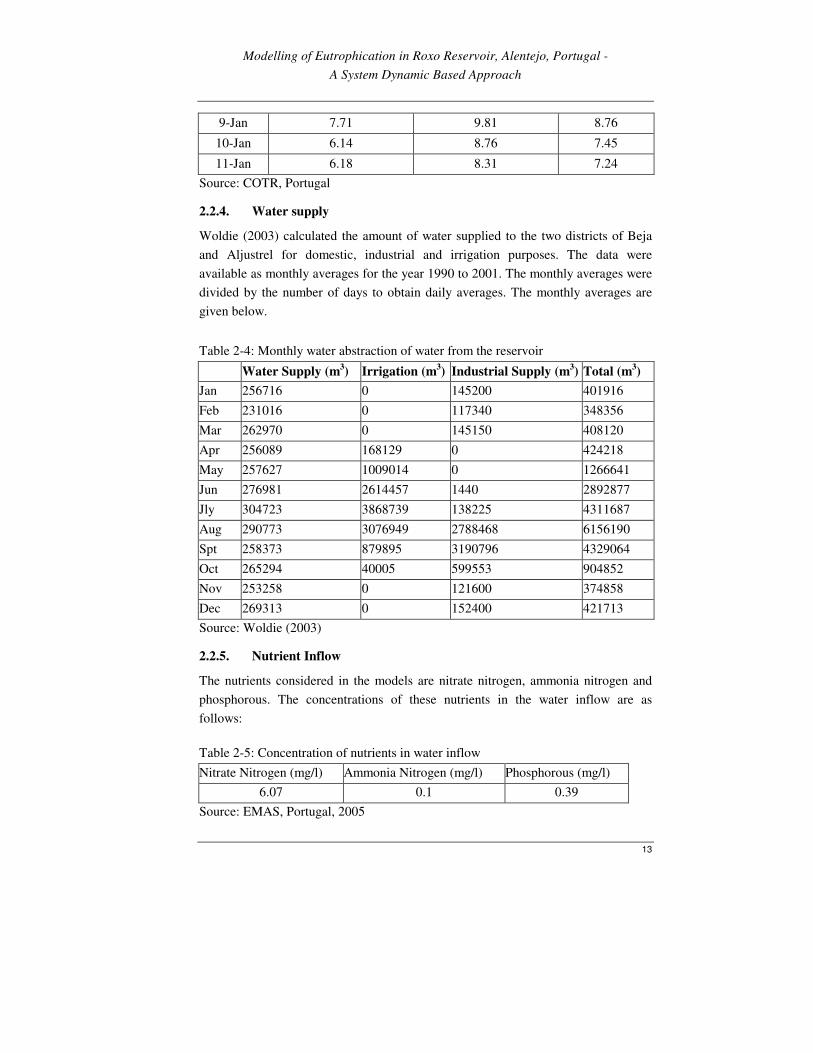
2.2.4. Water supply
Woldie (2003) calculated the amount of water supplied to the two districts of Beja
and Aljustrel for domestic, industrial and irrigation purposes. The data were
available as monthly averages for the year 1990 to 2001. The monthly averages were
divided by the number of days to obtain daily averages. The monthly averages are
given below.
Table 2-4: Monthly water abstraction of water from the reservoir
Water Supply (m3) Irrigation (m
3) Industrial Supply (m
3) Total (m
3)
Jan 256716 0 145200 401916
Feb 231016 0 117340 348356
Mar 262970 0 145150 408120
Apr 256089 168129 0 424218
May 257627 1009014 0 1266641
Jun 276981 2614457 1440 2892877
Jly 304723 3868739 138225 4311687
Aug 290773 3076949 2788468 6156190
Spt 258373 879895 3190796 4329064
Oct 265294 40005 599553 904852
Nov 253258 0 121600 374858
Dec 269313 0 152400 421713
Source: Woldie (2003)
2.2.5. Nutrient Inflow
The nutrients considered in the models are nitrate nitrogen, ammonia nitrogen and
phosphorous. The concentrations of these nutrients in the water inflow are as
follows:
Table 2-5: Concentration of nutrients in water inflow
Nitrate Nitrogen (mg/l) Ammonia Nitrogen (mg/l) Phosphorous (mg/l)
6.07 0.1 0.39
Source: EMAS, Portugal, 2005

Modelling of Eutrophication in Roxo Reservoir, Portugal –
A STELLA Based Approach
14
2.2.6. Evapotranspiration
Woldie (2003) calculated the monthly evapotranspiration from the different land
cover classes. The amount of evapotraspiration from water bodies was extracted.
This value was assumed to be the amount of evapotranspiration from the reservoir.
The average monthly evapotranspiration from the reservoir is as under.
Table 2-6: Average monthly evaporation from the reservoir
Month Evapotranspiration (m3)
Jan 611800
Feb 729400
Mar 1103200
Apr 1478400
May 1401400
Jun 1190000
Jly 1201200
Aug 844200
Spt 651000
Oct 523600
Nov 448000
Dec 578200
Source: Woldie (2003)
Modelling of Eutrophication in Roxo Reservoir, Alentejo, Portugal -
A System Dynamic Based Approach
15
3. Development and Description of Models
3.1. Model Development
Two casual loop diagrams were developed based on literature review and analysis of
the system. These diagrams were the basis on which the dynamic models were
developed. The fist diagram explains the basic factors that can affect the growth and
death of phytoplankton in the system and the second diagram explains the concept of
competition and toxicity between the two species. Definite system boundaries were
defined for both the diagrams and it was assumed that the elements outside these
boundaries were not relevant for the dynamic models. Description of these diagrams
is given in the following sections.
Three dynamic models were developed for the system. Model 1 was developed as a
calibration model. It was developed by assuming that only cyanobacteria was present
in the reservoir. This assumption was made to avoid interactions between species.
This model was used to check the suitability of the equations and to determine the
value of the different constants used in the dynamic models.
The second and the third dynamic models are more complex version of Model 1.
These models consider the presence of both cyanobacteria and C. hirundinela in the
reservoir. These models were developed to define the interactions between the
species. While Model 2 focuses on competition for resources (nutrients) between the
species, Model 3 also incorporates the effect of toxins released by C. hirundinela.
3.2. Basic causal loop diagram
The basic causal loop diagram for the system is given below.

Modelling of Eutrophication in Roxo Reservoir, Portugal –
A STELLA Based Approach
16
Figure 3-1: Causal loop diagram of the system
The description of the different components of diagram is given below
Water in the reservoir: The amount of water in the reservoir increases with water
inflow and decreases with outflow and evaporation.
Water Inflow: The amount of water flowing into the reservoir increases with the
amount of precipitation.
Nutrients Inflow: It is assumed that the only source of nutrient inflow is surface
runoff. As such, the amount of nutrients increases with the inflow of water in the
reservoir.

Modelling of Eutrophication in Roxo Reservoir, Alentejo, Portugal -
A System Dynamic Based Approach
17
Nutrient Outflow and Nutrient Consumption: Nutrients also flow out of reservoir
together with water. This outflow of depends on the nutrient concentration. Nutrients
are also reduced because of consumption by phytoplankton.
Phytoplankton Biomass: The phytoplankton biomass increases with the
phytoplankton growth and decreases with phytoplankton death.
Phytoplankton Growth: The growth of phytoplankton is affect largely by three
factors viz. sunlight, nutrients2 and temperature (Ryding et al, 1989). The growth rate
is also affected positively by birth (growth) rate and also by the phytoplankton
biomass.
Phytoplankton Death: Reduction in phytoplankton biomass is due to its death,
grazing by zooplankton and fish and endogenous respiration. The amount of grazing
is directly proportional to phytoplankton biomass. The death rate is also positively
affected by the death (mortality) rate and phytoplankton biomass.
3.3. Causal Loop Diagram for Competition and Toxicity
A causal loop diagram was developed specifically to represent competition and
toxicity between C. hirundinella and cyanobacteria. This diagram was used for the
designing of a competition equation for Model 2 and Model 3, and equation for
toxicity for Model 3. The different sections of the causal loop diagram for
competition and toxicity are as under.
Competition: The two species will compete for resources (nutrient). The
accessibility to resource for a species is reduced by the presence of the second
species. This reduction depends on the resource accessibility inhibition coefficient of
the species.
Toxicity: C. hirundinella can cause the death of cyanobaceria through release of
toxins. The extent of toxicity depends on the amount of C. hirundinella present as
well as the toxicity coefficient of C. hirundinella.
2 The element ‘Nutrients’ refers to the total of ammonia nitrogen, nitrate nitrogen and
phosphorous

Modelling of Eutrophication in Roxo Reservoir, Portugal –
A STELLA Based Approach
18
Figure 3-2: Causal loop diagram for competition and toxicity
3.4. Assumptions
A number of assumptions were made while translating the conceptual model to
STELLA models. These assumptions are:
1. The model assumes that the reservoir is treated as a continuously stirred tank. The
region experiences strong wind during most parts of the year. As such there is strong
wind driven current, which leads to mixing in most parts of the reservoir.
2. As the land use around the lake is predominantly agricultural, was assumed that
the only source of inflow of nutrients is from leaching of nutrients from these fields.
The point of discharge of municipal discharge is located at a sufficient distance from
the reservoir. This allows the rivers to recover and thus discharge a very small
amount of nutrients into the reservoir. Also because the area of the reservoir is very
small, atmospheric deposition of nutrients is also considered insignificant. It is also
assumed that the contribution of nutrients from the process of mineralization is
insignificant when compared to the direct inflow.
3. Although there is subsurface inflow of water during the wet season and a
subsurface outflow during summer, an assumption has also been made that ground
water has no significant influence on the volume of water stored in the reservoir.
This assumption has been made for purpose of simplification of the model.
4. While modeling competition and toxicity it was assumed that both the species
have the same birth and death rates and have the same temperature and light
requirement for growth.

Modelling of Eutrophication in Roxo Reservoir, Alentejo, Portugal -
A System Dynamic Based Approach
19
5. While modeling competition it was assumed that the presence one species of
phytoplankton will reduce the availability of resources for the other species.
6. It was assumed that the chlorophyll-a to biomass ratio is the same for both the
species.
3.5. Dynamic Models
Three different dynamic models with increasing levels of complexity were
developed. The development and the description of these models are described
below.
3.5.1. Model 1: Calibration
Model 1 was developed to check the suitability of the equations to describe the
different sections of the dynamic modes. It was also used to determine the values of
the constants in these models.
Selection of Equations
All the three STELLA models contain the following basic sections.
• Water in Reservoir
• Nutrients (Ammonium Nitrogen, Nitrate Nitrogen, Phosphorous)
• Light Limiting Factor
• Temperature Limiting Factor
• Nutrient Limiting Factor
• Phytoplankton Biomass
• Chlorophyll-a
All these sections are based on mathematical equations. The first model was
developed to check the suitability of different available equations to describe these
sections. The final equations describing these sections are as under.
Water in Reservoir: This section consists of four components viz.: inflow of water,
outflow of water, evaporation and water in the reservoir. The amount of water
flowing in and out of the reservoir is obtained from field observations and literatures.

Modelling of Eutrophication in Roxo Reservoir, Portugal –
A STELLA Based Approach
20
The values for these two components are entered manually into the software. The
amount of water in the reservoir can be modeled using the following equation
dWW WInflow WOutflow E
dt= + − − (3.1)
Where,
W = Water volume (m3)
WInflow = Amount of water flowing into the reservoir (m3/day)
WOutflow = Amount of water flowing out of the reservoir (m3/day)
E = Evapotranspiration (m3/day)
t = Time in days
Nutrient in the Reservoir: The nutrients considered in this project are Ammonia
Nitrogen, Nitrate Nitrogen and Phosphorous. The change in the amount of these
nutrients in the reservoir is calculated using the following equation (Modified from
ITC, 2000).
[ ( *1000)* Re *( *1000) * * * * ]dN
N WInflow ConcInflow Conc servoir WOutflow PB LLF NuLF TLF MGRdt
= + − −
(3.2)
Where,
N = Amount of nutrients in the reservoir (mg)
WInlfow = Water inflow (m3/day)
ConcInflow = Concentration of the nutrients in water inflow (mg/l)
ConcResrvoir = Concentration of the nutrients in the reservoir (mg/l)
WOutlfow = Water outflow (m3/d)
PB = Phytoplankton biomass (mg)
LLF = Light limiting factor
TLF = Temperature limiting factor
NuLF = Nutrient limiting factor
MGR = Maximum growth rate
Light Limiting Factor: The light limiting factor tends to be close to unity when the
light intensity is close to the optimal temperature required for phytoplankton growth.
Deviation from the optimal light intensity in either direction will reduce the value of

Modelling of Eutrophication in Roxo Reservoir, Alentejo, Portugal -
A System Dynamic Based Approach
21
the limiting factor. The value of the factor can be calculated using the following
equation (Pelletier, 1999).
(1)*
LIOLILI e
LLFOLI
−
= (3.3)
Where,
LLF = Light limiting factor
LI = Light intensity (W/m2)
OLI = Optimal light intensity (W/m2)
Temperature Limiting Factor: Similar to the light limiting factor, the value of
temperature limiting factor tends to unity when the temperature is close to optimal
temperature. Deviation from the optimal temperature in either direction will reduce
the value of the limiting factor. The value of the factor is calculated using the
following equation (Beckers, 1999)
2
2*(1 )*
( 2* * 1)
SF XtTLF
Xt SF Xt
+=
+ +
(3.4)
Where,
TLF = Temperature limiting factor
SF = Shape factor
And,
T OTXt
OT Lt
−=
− (3.5)
Where,
T = Temperature (ºC)
OT = Optimal temperature for phytoplankton growth (ºC)
LT = Low lethal temperature (ºC)

Modelling of Eutrophication in Roxo Reservoir, Portugal –
A STELLA Based Approach
22
Nutrient Limiting Factor: The nutrient limiting factor is the minimum of the
phosphorous limiting factor and the sum of nitrate and ammonia limiting factor
(Modified from ITC, 2000; Beckers, 1999).
min[ , ( )]NuLF PLF NLF ALF= + (3.6)
Where,
NuLF = Nutrient limiting factor
PLF = Phosphorous limiting factor
NLF = Nitrate limiting factor
ALF = Ammonia limiting factor
The phosphorous, nitrate and ammonia limiting factors are calculated as follows
(ITC, 2000)
PconcPLF
Pconc KP=
+
(3.7)
AconcALF
Aconc KA=
+
(3.8)
( * )* APF AconcNconc e
NLFNconc KN
−
=
+
(3.9)
Where,
PLF = Phosphorous Limiting Factor
Pconc = Concentration of phosphorous in the reservoir (mg/l)
KP = Monod constant for phosphorous (mg P/l)
ALF = Ammonia limiting factor
Acon = Concentration of ammonia in the reservoir (mg/l)
KA = Monod constant for ammonia (mg N/l)
NLF = Nitrate limiting factor
Nconc = Concentration of nitrate in the reservoir (mg/l)
APF = Ammonia Preference Factor
KN = Monod constant for nitrate (mg N/l)
Modelling of Eutrophication in Roxo Reservoir, Alentejo, Portugal -
A System Dynamic Based Approach
23
Chlorophyll-a: The amount of chlorophyll-a in the reservoir is a function of the
phytoplankton biomass. The total chlorophyll-a content can be calculated using the
following equation.
( *1000)*Chloro TPB ChloroPigment= (3.10)
Where,
Chloro = Chlorophyll-a content (µg)
TPB = Total phytoplankton biomass (mg)
ChloroPigment = Amount of chlorophyll-a pigment per unit
phytoplankton biomass (µg / µg)
The concentration of chlorophyll-a can be calculated using the following equation.
( *1000)
ChloroChloroConc
W= (3.11)
Where,
ChloroConc = Chlorophyll-a concentration (µg /l)
Chloro = Total chlorophyll-a in reservoir (µg)
W = Total water in reservoir (m3)
Phytoplankton Biomass: This section has three main components viz.:
phytoplankton growth, phytoplankton death, and phytoplankton biomass in the
reservoir. The change in phytoplankton biomass is given by the following equation
(Modified from ITC, 2000; Beckers, 1999).
( 20)[1 * * * * ]TdPBPB MGR LLF TLF NLF DR GR RRC TCR
dt
−
= + − − −
(3.12)
Where
PB = Phytoplankton biomass (mg/l)
MGR = Maximum growth rate
LLF = Light limiting factor
TLF = Temperature limiting factor
NLF = Nutrient limiting factor
DR = Death rate

Modelling of Eutrophication in Roxo Reservoir, Portugal –
A STELLA Based Approach
24
GR = Grazing rate
RRC = Respiration rate constant
TCR = Temperature constant for respiration for respiration
T = Temperature (ºC)
Values of Constants
The values of the different constants used in the models were approximated in Model
1. The constants and their respective values are given below.
Table 3-1: Constants used in the models and their values
S. No Constant Value Units
1 Monod constant for nitrate nitrogen 0.001 mg N/l
2 Monod constant for ammonia nitrogen 0.001 mg N/l
3 Monod constant for phosphorous 0.001 mg P/l
4 Ammonia preference factor 1.46 mg N/l
5 Optimal light intensity 250 W/m2
6 Optimal temperature 23 º C
7 Shape factor for temperature limiting factor -0.6 ---
8 Lowermost threshold for temperature 5 º C
9 Maximum growth rate 0.9 day -1
10 Grazing rate 0.265 day -1
11 Death rate 0.3 day -1
12 Respiration rate 0.1 l/d
13 Temperature coefficient for respiration 1 ---
3.5.2. Model 2: Competition between Species
Model 2 considers the presence of both cyanobacteria and C. hirundinella in the
reservoir. This model consists of all the basic sections as above and a section on
competition between the species. The purpose of this model was to develop an
equation to model competition between the two species. The equation was developed
assuming that the presence of one species would reduce the accessibility to resources
of the second species. The resource considered in this model was nutrient.
1 1*
n n nRNLF B NIC
− −= (3.13)

Modelling of Eutrophication in Roxo Reservoir, Alentejo, Portugal -
A System Dynamic Based Approach
25
Where,
RNLF = Reduced nutrient limiting factor
n = Species 1 and 2
B = Biomass (µg)
NIC = Nutrient inhibition coefficient
The values of nutrient inhibition coefficient for the two species are as under.
Table 3-2: Nutrient inhibition coefficient of the two species
Species Nutrient inhibition coefficient Value
Cyanobacteria 112*10
−
C. hirundinela 111.8*10
−
The equation on phytoplankton biomass was modified to incorporate the change in
the nutrient limiting factor. The modified equation is as follow.
( 20)[1 * * * * ]TndPB
PB MGR LLF TLF RNLF DR GR RRC TCRdt
−
= + − − −
(3.14)
Where,
PB = Phytoplankton biomass (mg/l)
N = Species 1 and 2
MGR = Maximum growth rate
LLF = Light limiting factor
TLF = Temperature limiting factor
RNLF = Reduced nutrient limiting factor
DR = Death rate
GR = Grazing rate
RRC = Respiration rate constant
TCR = Temperature constant for respiration for respiration
T = Temperature (ºC)
3.5.3. Model 3: Toxicity
Model 3 is a more complex version of Model 2 and will be treated as the final
model. This model also incorporates toxicity to the system. According to Rodriguez
(2003) C. hirundinela is toxic by nature and its presence in substantial quantities can

Modelling of Eutrophication in Roxo Reservoir, Portugal –
A STELLA Based Approach
26
lead to fish kills. Considering this, it has been assumed in this model that C.
hirundinela will release toxins which would lead to death in cyanobacteria. The
amount of toxic material released was calculated using the following equation.
*TTR ToxicityCoeff BCH= (3.15)
Where,
TTR = Total toxin released (mg)
BCH = Biomass of C. hirundinela (mg)
ToxicityCoeff = Coefficient of toxicity
A detail parametric chart of the model is given in Annex 4.
3.6. Model Limitations
3.6.1. Phytoplankton Growth during the First 135 days
One limitation of the model is that it assumes that there is no change in the
chlorophyll-a concentration during the first 135 days. The models predict very low
values of both light and temperature limiting factors in this phase and therefore
survival of phytoplankton would not be possible. However, available ground data
showed average chlorophyll-a concentration of 13.5 µg/l indicating presence of
phytoplankton during this phase.
The presence can be attributed to the adaptability of phytoplankton which enables
them to survive on low temperature and light. Although modeling this adaptability
was possible, it will not only require very detailed information on the phytoplankton
species but will increase the complexity of the models. To overcome this problem it
was assumed that there will be some phytoplankton present in the system but no
change in their biomass will occur during this phase; the biomass was adjusted to
yield an average chlorophyll concentration of 13 µg/l. Because of this assumption,
the model is not capable of prediction variation in the phytoplankton biomass or
chlorophyll-a concentration in this phase.
3.6.2. Model Efficiency
Very little of ground data were available to validate the model. Although correlation
and root mean square analysis was done, it was not possible to determine the
efficiency of the model because of limited data.

Modelling of Eutrophication in Roxo Reservoir, Alentejo, Portugal -
A System Dynamic Based Approach
27
3:07 PM Sun, Jan 28, 2007
Untitled
Page 1
1.00 92.00 183.00 274.00 365.00
Day s
1:
1:
1:
25000000
40000000
55000000
1: Water in Reserv oir
1
1
1
1
7:32 PM Wed, Feb 07, 2007
Untitled
Page 1
1.00 92.00 183.00 274.00 365.00
Day s
1:
1:
1:
2:
2:
2:
0
400000
800000
0
100000
200000
1: Water Inf low 2: Water Outf low
1
1 1
12 2
2
2
4. Basic Model Outputs
4.1. Water in the Reservoir
The daily variation in the volume of water in the reservoir as predicted by Model 3 is
as under.
Figure 4-1: Variation of water volume (m3) with time in the reservoir
The volume of water is dependent on two factors viz. water inflow and water
outflow. These factors are as under.
Figure 4-2: Water inflow (m3/d) and water outflow (m
3/d)

Modelling of Eutrophication in Roxo Reservoir, Portugal –
A STELLA Based Approach
28
3:26 AM Sun, Feb 04, 2007
Untitled
Page 1
1.00 92.00 183.00 274.00 365.00
Day s
1:
1:
1:
0
1
1
1: Nutrient Limit ing Factor
1 1 1 1
4.2. Limiting Factors
4.2.1. Nutrient Limiting Factor
The variation in nutrient limiting factor as predicted by Model 3 is given below.
Figure 4-3: Variation in nutrient limiting factor
From figure 4.3 it can be seen that the value of the nutrient limiting factor is 1 for
most parts of the year. Change in the value of the limiting factor was seen only
during the time period between mid-October and mid-November. During this period
the value was fluctuating between 0.98 and 0.19.
The change in the nutrient limiting factor is governed largely by a change in the
amount of nutrients present in the reservoir, which in turn is influenced by nutrient
outflow and nutrient consumption. The nutrient outflow and consumption as
predicted by the Model 3 are as under.

Modelling of Eutrophication in Roxo Reservoir, Alentejo, Portugal -
A System Dynamic Based Approach
29
7:35 PM Wed, Feb 07, 2007
Untitled
Page 1
1.00 92.00 183.00 274.00 365.00
Day s
1:
1:
1:
2:
2:
2:
0
1.5e+010
3e+010.
0
2.5e+011
5e+011.
1: Total nutrients consumed 2: Total nutrient outf low
11
1
1
2 2
2
2
7:38 PM Wed, Feb 07, 2007
Untitled
Page 1
1.00 92.00 183.00 274.00 365.00
Day s
1:
1:
1:
6e+013.
9e+013.
1.2e+014
1: Total nutrient in the Reserv oir
11
1
1
Figure 4-4: a) Nutrient outflow and nutrient consumed; b) Variation in total nutrient
content
It can be seen from figure 4.4 a) that the outflow of nutrients is high during summer
when water abstraction is high and that nutrient consumption is high in June and
October-November. These time periods correspond to high phytoplankton biomass
in the reservoir. From figure 4.4 b), it can be seen that the nutrient in the reservoir is
reduced significantly by October. This reduction in nutrient concentration leads to
reduction in the nutrient limiting factor.
4.2.2. Light Limiting Factor
The variation in light limiting factor as predicted by Model 3 is given below.

Modelling of Eutrophication in Roxo Reservoir, Portugal –
A STELLA Based Approach
30
2:16 PM Sun, Jan 28, 2007
Untitled
Page 1
1.00 92.00 183.00 274.00 365.00
Day s
1:
1:
1:
0.329
0.7145
1.1
1: Light Limiting Factor
1
11
1
12:46 AM Tue, Feb 13, 2007
Untitled
Page 1
1.00 92.00 183.00 274.00 365.00
Day s
1:
1:
1:
0.3
0.65
1.
1: Temperature Limiting Factor
1
11
1
Figure 4-5: Variation in light limiting factor
The area receives very little light in the winter season. As such, there is not enough
light for the growth of phytoplankton species in the reservoir. The value of light
limiting factor is very small indicating that light is a limiting factor in this period.
The factor however tends towards 1 in summer indicating that there is sufficient light
available for phytoplankton growth.
4.2.3. Temperature Limiting Factor
The variation in the temperature limiting factor is given below.
Figure 4-6: Variation in temperature limiting factor
Figure 4.6 shows two distinct peaks in the temperature limiting factor. The respective
average values at the first and the second peaks are 0.97 and 0.95. The value is

Modelling of Eutrophication in Roxo Reservoir, Alentejo, Portugal -
A System Dynamic Based Approach
31
1:43 PM Mon, Feb 12, 2007
Untitled
Page 1
1.00 92.00 183.00 274.00 365.00
Day s
1:
1:
1:
2:
2:
2:
10
25
40
22
23
24
1: Temperature 2: Optimal Temperature
1
1
1
12 2 2 2
moderately low in summer with an average value of 0.7 and extremely low in winter
with an average value of 0.5. The low values of temperature in peak summer and
peak winter indicates that temperature is one of the limiting factors during these
periods.
The optimal temperature for the growth of phytoplankton was assumed to be 23ºC.
In winter, the average temperature of the region is about 12 ºC, which is far below
the optimal temperature. The temperature limiting factor therefore has an extremely
low value during winter. In summer the average temperature of the region is 33 ºC.
It is this deviation from optimal temperature that results in the moderately low value
of the temperature limiting factor.
Figure 4-7: Variation in temperature and optimal temperature

Modelling of Eutrophication in Roxo Reservoir, Portugal –
A STELLA Based Approach
32

Modelling of Eutrophication in Roxo Reservoir, Alentejo, Portugal -
A System Dynamic Based Approach
33
3:31 AM Sun, Feb 04, 2007
Untitled
Page 1
1.00 92.00 183.00 274.00 365.00
Day s
1:
1:
1:
0
150
300
1: Chlorophy ll a Concntration
1 1
1 1
5. Estimation of Eutrophication Extent
5.1. Method
The chlorophyll-a concentration as predicted by Model 3 was noted. The average
and the maximum chlorophyll-a concentration were extracted. These values were
then compared to the threshold limits prescribed by Ryding et al (1989) and
Chapman (1992).
5.2. Results
The variation in chlorophyll-a concentration is as under.
Figure 5-1: Variation in Chlorophyll-a concentration (in µg /l) with time
The result shows significant amount of variation in the chlorophyll-a concentration
between the time period of mid-October and first week of December. A sharp
increase in the concentration is observed from mid-October. The concentration rises
until the maximum value is attained in the first week of November; it then declines
rapidly and becomes zero in the first week of December.
The average annual and the maximum chlorophyll-a concentration are given below.

Modelling of Eutrophication in Roxo Reservoir, Portugal –
A STELLA Based Approach
34
Figure 5-2: Average annual and maximum chlorophyll-a concentration
Average Annual Concentration (µg /l) Maximum Concentration (µg /l)
30.18 255.13
The results were then compared with the prescribed threshold limits. It was found
that the reservoir is eutrophic based on the average annual concentration and
hypertrophic based on the maximum concentration values.

Modelling of Eutrophication in Roxo Reservoir, Alentejo, Portugal -
A System Dynamic Based Approach
35
7:45 PM Wed, Feb 07, 2007
Untitled
Page 1
1.00 92.00 183.00 274.00 365.00
Day s
1:
1:
1:
2:
2:
2:
0
2.5e+009
5e+009.
0
1e+010.
2e+010.
1: Cy anobacteria 2: C hirundinela
1 1
1
12 2 2
2
6. Variation in the Biomass of Cyanobacteria and C. hirundinela
6.1. Method
The biomass of cyanobacteria and C. hirundinela was simulated in both Model 2 and
Model 3. Visual analysis was performed to understand the variation of these species.
6.2. Results
6.2.1. Variation Predicted by Model 2
Figure 6-1: Variation in the biomass of Cyanobacteria and C. hirundinela as
predicted by Model 2
Note: Different scales on the ‘Y axis’
Model 2 assumes that competition for nutrients is the only form of intersection
between the two species. As per this model cyanobacteria is the more dominant
species in the reservoir.
Model 2 results show that the biomass of C. hirundinela is at the maximum during
the first week of June. From the second week of June a decline in C. hriundinela
biomass is predicted. The decrease is primarily due to reduced accessibility to
nutrients. It is also predicted that the biomass becomes zero only in the month of
December.

Modelling of Eutrophication in Roxo Reservoir, Portugal –
A STELLA Based Approach
36
7:45 PM Wed, Feb 07, 2007
Untitled
Page 1
1.00 92.00 183.00 274.00 365.00
Day s
1:
1:
1:
2:
2:
2:
0
2.5e+009
5e+009.
0
1e+010.
2e+010.
1: Cy anobacteria 2: C hirundinela
1 1
1
12 2 2
2
Results of this model shows that biomass of cyanobacteria is the highest in the month
of November. There is also a relatively small increase in the biomass during the first
week of June.
6.2.2. Variation Predicted by Model 3
Figure 6-2: Variation in the biomass of Cyanobacteria and C. hirundinela as
predicted by Model 3
Note: Different scales on the ‘Y axis’
Model 3, which incorporates both toxicity and competition for nutrients, shows that
C. hirundinla is the more dominant species. The trend in the variation in the biomass
of the two species was found to be the opposite of that predicted by Model 2. The
biomass of cyanobacteria reaches the maximum during the first week of June. From
the second week of June a decline in the biomass is predicted. The decrease is
primarily due to toxicity. It is also predicted that the biomass becomes zero only in
the month of October.
Results of this model shows that biomass of C. hirundinela is the highest in the
month of November. There is also a relatively small increase in the biomass during
the first week of June.
Because the introduction of toxicity made C. hirundinela the more dominating
species inspite of the competition, it can be stated here that toxicity is the stronger of
the two intersections.

Modelling of Eutrophication in Roxo Reservoir, Alentejo, Portugal -
A System Dynamic Based Approach
37
8:03 PM Wed, Feb 07, 2007
Untitled
Page 1
1.00 92.00 183.00 274.00 365.00
Day s
1:
1:
1:
2:
2:
2:
0
1e+010.
2e+010.
0.329
0.7145
1.1
1: Cy anobacteria 2: Light Limiting Factor
1 1
1
1
2
2
2
2
7. Most Influencing Factor
7.1. Method
Apart from the three factors, the growth of both the species are also affected by the
interactions between the species. To remove the effect of these interactions, an
alternate scenario (Scenario 1) was created in Model 3 where it was assumed that the
presence one species does not affect the growth of the second species. Since the
growth and death rate of both the species are the same the growth of both the species
would be similar in this scenario. The model was executed and the result was
visually interpreted to determine the influencing factors. Visual interpretation was
done since the factors were becoming limiting during different phases of the year and
as such statistical analysis was not possible.
7.2. Results
The results of Scenario 1 are as follows.
Figure 7-1: Variation in cyanobacteria biomass and light limiting factor under
Scenario 1

Modelling of Eutrophication in Roxo Reservoir, Portugal –
A STELLA Based Approach
38
8:05 PM Wed, Feb 07, 2007
Untitled
Page 1
1.00 92.00 183.00 274.00 365.00
Day s
1:
1:
1:
2:
2:
2:
0
1e+010.
2e+010.
0.3
0.65
1.
1: Cy anobacteria 2: Temperature Limiting Factor
1 1
1
1
2
2
2
2
8:06 PM Wed, Feb 07, 2007
Untitled
Page 1
1.00 92.00 183.00 274.00 365.00
Day s
1:
1:
1:
2:
2:
2:
0
1e+010.
2e+010.
0.1
0.55
1.
1: Cy anobacteria 2: Nutrient Limiting Factor
1 1
1
1
2 2 2
2
Figure 7-2: Variation in cyanobacteria biomass and temperature limiting factor under
Scenario 1
Figure 7-3: Variation in cyanobacteria biomass and nutrient limiting factor under
Scenario 1
From the results of the scenario it can be seen that there is a fluctuation in the
biomass during summer (140 – 275 days). A decline in the biomass is observed in

Modelling of Eutrophication in Roxo Reservoir, Alentejo, Portugal -
A System Dynamic Based Approach
39
the subsequent phase. The decline was very rapid on the onset of winter but gradual
towards the end of the year.
A visual analysis of the results shows that the fluctuation in the biomass in summer is
because of changes in the temperature limiting factor. The value of both light and
nutrient limiting factor changes very little during this phase. It can thus be said that
temperature is the most limiting factor in summer.
The steep decline in the biomass was seen to correspond with a fall in the nutrient
limiting factor value. The changes in the light and temperature limiting factor was
found to be very little. Thus it was inferred that nutrient becomes the limiting factor
on the onset of winter.
The gentle decline corresponds to the drop in the values of temperature and light
limiting factors. The value of nutrient limiting factor was found to be more or less
constant during this phase. Thus, it was inferred that the growth of phytoplankton is
limited by both light and temperature towards the end of the year.

Modelling of Eutrophication in Roxo Reservoir, Portugal –
A STELLA Based Approach
40

Modelling of Eutrophication in Roxo Reservoir, Alentejo, Portugal -
A System Dynamic Based Approach
41
8. Effect of Abstraction
8.1. Method
In the baseline scenario, the change in chlorophyll-a concentration is due to change
in both chlorophyll-a content and water volume; reduction in the water volume will
lead to higher concentration. Reduction in water is because of evapotranspiration and
abstraction. While evapotranspiration is a natural process, reduction in water volume
due to abstraction is anthropogenic.
To determine the effect of abstraction an alternate scenario (Scenario 2) was
developed assuming that there was no withdrawal of water. The difference between
the alternate scenario and the baseline scenario is reduction of water volume due to
abstraction. If the chlorophyll-a concentration from this scenario is subtracted from
the predicted values, the residue will be the effect of abstraction on chlorophyll-a
concentration. Graphically, the concept can be represented as follows.
Figure 8-1: Method to determine the effect of abstraction
Percentage difference was obtained to determine the contribution percentage of
abstraction on total chlorophyll-a concentration.
Time (days)
Time = t
Ch
loro
ph
yll
-a c
on
cen
trat
ion
(µ
g/l
)
Effect of
Abstraction
at time = t
Baseline Scenario
Scenario 2

Modelling of Eutrophication in Roxo Reservoir, Portugal –
A STELLA Based Approach
42
8:12 PM Wed, Feb 07, 2007
Untitled
Page 1
1.00 92.00 183.00 274.00 365.00
Day s
1:
1:
1:
2:
2:
2:
25000000
40000000
55000000
0
100000
200000
1: Water in Reserv oir 2: Abstraction
1
1
1
1
2 2
2
2
8.2. Results
The change in water volume and abstraction in the reservoir is given below.
Figure 8-2: Change in water volume (m3) and abstraction (m
3/d)
It can be seen from the figure above that the volume of water decreases considerably
in the dry seasons, especially in the months August to October. This change is
because of abstraction of water from the reservoir. It is expected that the low water
volume during these months will contribute significantly to the concentration of
chlorophyll-a in the reservoir.
The result of the analysis to determine the effect of water abstraction on chlorophyll-
a concentration is given below:
Table 8-1: Average monthly contribution of abstraction
Month
Contribution of
abstraction (µg/l)
Percentage contribution
of abstraction (%)
Jan 0.05 0.38
Feb 0.14 1.11
Mar 0.23 1.80
Apr 0.22 1.72
May 1.06 4.14
Jun 4.24 8.24
Jul 4.74 15.58

Modelling of Eutrophication in Roxo Reservoir, Alentejo, Portugal -
A System Dynamic Based Approach
43
Aug 2.58 26.57
Sep 6.70 37.99
Oct 28.12 42.81
Nov 50.77 53.10
It can be seen from the table that the water abstraction does affect the concentration
of chlorophyll-a in the reservoir especially during the dry season. Maximum effect
was seen in the month of November when the water volume was significant low. The
effect of abstraction is also very high in the months of September and October.
The analysis was not applicable for the month of December because the chlorophyll-
a concentration is zero in most days of the month.

Modelling of Eutrophication in Roxo Reservoir, Portugal –
A STELLA Based Approach
44

Modelling of Eutrophication in Roxo Reservoir, Alentejo, Portugal -
A System Dynamic Based Approach
45
9. Comparison of Model Output with Measured Data
9.1. Method
Correlation and root mean square error analysis was performed to check how well
Model 3 describes the variation of chlorophyll-a concentration in the system.
Analysis was done between chlorophyll-a concentration as observed on the ground
data and chlorophyll-a concentration as predicted by Model 3.
The ground dataset contains a limited number of observations from the years 2002,
2003 and 2004. Correlation and RMSE analysis was done for each year separately. A
portion of the available ground data is below.
Table 9-1: A portion of the available data on chlorophyll-a concentration
Date
Chlorophyll-a
Concentration
(µg/l) for 2002
Chlorophyll-a
Concentration (µg
/l) for 2003
Chlorophyll-a
Concentration (µg
/l) for 2004
7-Jan 36.98
8-Jan 9.8
13-Jan 12.65
4-Feb 30.06
5-Feb 1.9
10-Feb 35.27
5-Mar 2.11
5-Mar 4.16
9-Mar 3.92
1-Apr 3.32
2-Apr 1
6-Apr 8.17
4-May 34.77
6-May 12.96
7-May 5.71
Source: EMAS, 2005

Modelling of Eutrophication in Roxo Reservoir, Portugal –
A STELLA Based Approach
46
The available ground data was found to be of non-Gaussian distribution form; the
total number of observations for the years 2002, 2003 and 2004 are 12, 10 and 12,
respectively. Therefore, Spearman’s Rank Order Test was used to determine the
correlation.
The root mean square error (RMSE) analysis was done to check if the values of
chlorophyll-a concentration predicted by Model 3 deviated for the ground data.
RMSE was checked for each of the three years. The equation used for checking the
RMSE is as follows:
2
1
1[ ( )
n
RMSE CCg CCmn
= −∑ (9.1)
Where
RMSE = Root Mean Square Error
CCg = Chlorophyll-a concentration from ground data
CCm = Chlorophyll-a concentration from model data
n = Number of observation
Because the available ground data was non-Gaussian, outliers present in the data
could not be identified. Presence of outliers can affect the result of the correlation
and RMSE analysis. The result of the analysis can be improved by reducing the
effect of these outliers. One technique of reducing their effect is by averaging.
It can be seen that the observations are from similar dates (in different years). The
values of chlorophyll-a concentration from these dates were combined to get average
concentrations. Averages from the corresponding dates were obtained from the
Model 3 result. Correlation and RMSE analysis was performed between the averaged
data sets. A portion of the averaged ground data and averaged Model 3 results are
given below. Available and averaged ground data is provided Annex 5. Averaged
Model 3 output is provided in Annex 6.

Modelling of Eutrophication in Roxo Reservoir, Alentejo, Portugal -
A System Dynamic Based Approach
47
Table 9-2: Portion of the averaged ground data on chlorophyll-a concentration
S
No. Date
Chlorophyll-a
Concentration
(µ gram/l) for
2002
Chlorophyll-a
Concentration
(µ gram/l) for
2003
Chlorophyll-a
Concentration
(µ gram/l) for
2004
Average
Chlorophyll-a
Concentration
(µ gram/l)
7-Jan 36.98
8-Jan 9.8 1
13-Jan 12.65
19.81
4-Feb 30.06
5-Feb 1.9 2
10-Feb 35.27
22.41
5-Mar 2.11
5-Mar 4.16 3
9-Mar 3.92
3.40
1-Apr 3.32
2-Apr 1 4
6-Apr 8.17
4.16
4-May 34.77
6-May 12.96 5
7-May 5.71
17.81
Source: EMAS,2005
Table 9-3: Portion of the averaged Model 3 output
S. No Date
Daily Chlorophyll –a
Concentration (µg/l)
Average Chlorophyll –a
Concentration (µg/l)
7-Jan 12.98
8-Jan 12.93 1
13-Jan 12.93
12.95
4-Feb 12.87
5-Feb 12.88 2
10-Feb 12.90
12.88
5-Mar 12.68 3
9-Mar 12.73 12.71
1-Apr 12.48 4
2-Apr 12.45
12.47

Modelling of Eutrophication in Roxo Reservoir, Portugal –
A STELLA Based Approach
48
6-Apr 12.47
4-May 12.51
6-May 12.56 5
7-May 12.58
12.55
Because the average data were obtained by combining data from different years, the
total number of readings remains the same. As such improvement in the correlation
and RMSE value are because of removal of outliers only.
9.2. Results and Discussion
A graphical comparison of Model 3 results was done with the ground data from each
of the years as well as with the averaged ground data. The results are as under.
Figure 9-1: Comparison between ground data for 2002 and Model 3 results
Ground data from 2002 and Model 3 results
0
50
100
150
200
250
1 2 3 4 5 6 7 8 9 10 11 12
Ch
loro
ph
yll
-a c
on
cn
etr
ati
on
(mic
rog
ram
s/l
)
Ground Data
Model 3 Output

Modelling of Eutrophication in Roxo Reservoir, Alentejo, Portugal -
A System Dynamic Based Approach
49
Figure 9-2: Comparison between ground data for 2003 and Model 3 results
Figure 9-3: Comparison between ground data for 2004 and Model 3 results
Ground data from 2003 and Model 3 results
0
50
100
150
200
1 2 3 4 5 6 7 8 9 10
Ch
loro
ph
yll-a
co
ncen
trati
on
(mic
rog
ram
s/l)
Ground Data
Model 3 Results
Ground data from 2004 and Model 3 results
0
50
100
150
200
1 2 3 4 5 6 7 8 9 10 11 12
Ch
loro
ph
yll
-a c
on
cen
trati
on
(mic
rog
ram
s/l
)
Ground Data
Model 3 Results

Modelling of Eutrophication in Roxo Reservoir, Portugal –
A STELLA Based Approach
50
Figure 9-4: Comparison between averaged ground data and Model 3 results
Correlation and RMSE test was done between the ground data and the results of
Model 3. The results are as follows.
Table 9-4: Result of the correlation and RMSE analysis
Ground Data from Year Correlation with Model Output RMSE (µg/l)
2002 0.40 27.7
2003 0.45 30.1
2004 0.40 57.7
Combined Average 0.54 20.2
Results show positive correlation for all the three years as well as for the combined
data. Correlation was moderately good when each year were considered separately.
The correlation improved when for the averaged data. The root mean square analysis
show low values for the years 2002 and 2003 and high value year 2004. However,
the error was found to be low for the averaged data.
The low correlation and high RMSE values for the yearly data are mainly because of
following two factors.
a) Limited number of observation in the ground data
b) Presence of outliers in the ground data
Average ground data and Model 3 results
0
2040
60
80100
120
140160
180
1 2 3 4 5 6 7 8 9 10 11 12
Ch
loro
ph
yll
-a c
on
cen
trati
on
(mic
rog
ram
/l)
Averaged Ground Data
Model 3 Results

Modelling of Eutrophication in Roxo Reservoir, Alentejo, Portugal -
A System Dynamic Based Approach
51
Limited Observations: The total number of observations for the years 2002, 2003
and 2004 are 12, 10 and 12 respectively. Statistically the observations are not
adequate for assessing either correlation or RMSE. As such, it can be argued here
that the result of the analysis does not indicate the actual efficiency of the model in
describing the system. It is expected here that adequate amount of data will not only
assess better assess the efficiency of the model.
Outliers: Because of the limited observation outliers in the data cannot be identified.
Presence of outliers can result in low correlation high RMSE. The effect of outliers
can be negated to some extent when average values are considered. It can be seen
from the result that a combined average yield better correlation and RMSE values.
As such, it can be expected that an average ground data will improve the correlation
and RMSE values.

Modelling of Eutrophication in Roxo Reservoir, Portugal –
A STELLA Based Approach
52

Modelling of Eutrophication in Roxo Reservoir, Alentejo, Portugal -
A System Dynamic Based Approach
53
10. Conclusion and Recommendaion
10.1. Conclusion
Although we are fully aware of the complexity of the ecology of lake ecosystems
and especially the behaviour and dynamics of phytoplankton (Huisman et al, 1999),
we tried to better understand the mechanism of eutrophication and algal bloom in an
important water reservoir in south Portugal, using available monitoring data of water
authorities (ABROXO, COTR, EMAS, ADRHA, INETI, 3).
Extent of eutrophication
The average annual chlorophyll-a concentration was found to be 30.18 µg/l. As per
the results of Model 3, the maximum chlorophyll-a concentration was about 255.13
µg/l. From these results it can be concluded that the reservoir is hypertrophic. These
values correspond more or less to the observed chlorophyll-a levels and variations.
Variation in the biomass of cyanobacteria and Ceratium hirundinella
The result of Model 3 shows that the maximum biomass of cyanobacteria is obtained
in the month of June. The biomass then decreases through the rest of the year until it
becomes zero in the month of December. For C. hirundinela, there is a slight
increase in the biomass during the month of June. The biomass then decreases
gradually until the month of October. During this month the rate of growth is very
high. Highest biomass is predicted for the month of November.
3 ABROXO: Association of Beneficiaries of the Roxo reservoir & irrigation area,
Montes Velhos, Alentejo, Portugal.
COTR: Centre for Irrigation Technology, Beja, Portugal.
EMAS: Municipal Water Supply & Sanitation Authority, Beja, Portugal.
IDRHA: Institute of Rural Development and Hydraulics, Ministry of Agriculture,
Rural Development and Fisheries, Lisbon, Portugal
INETI: National Institute of Engineering, Technology & Innovation, Lisbon,
Portugal
Modelling of Eutrophication in Roxo Reservoir, Portugal –
A STELLA Based Approach
54
Most influencing factor
Temperature was found to be the most dominating factor that can affect the growth
of both cyanobacteria and Ceratium hirundinela in the reservoir during summer. It
was also seen that nutrient becomes the most limiting factor on the onset of winter.
Towards the end of the year, both temperature and light were found to be the limiting
factors.
Effect of abstraction
The maximum effect of abstraction was seen in the month of November when the
water volume was significant low. The effect of abstraction is also very high in the
months of September and October.
10.2. Recommendation
10.2.1. Observation Density
To better understand the variation in the variation in the biomass of cyanobacteria
and C. hirundinela, it is recommended that daily observation on chlorophyll-a
concentration be carried out. A specific time of sampling would also lead to better
observation.
Individual observations on chlorophyll-a concentration could correspond to
outstanding meteorological and ecological conditions. These values can then be
treated as outliers. To remove the effect of these outliers, average daily chlorophyll-a
concentration should be taken. It is recommended that the average be obtained by
combining data from at least three consecutive years.
Observation on dissolved oxygen content is also recommended. Observation should
be carried out together with chlorophyll-a. The presence of dissolved oxygen data
would enable quantification of the effect of eutrophication on the reservoir.
10.2.2. Ecological Study
Though an effort was made in this project to understand the interaction between the
species, it was not possible to quantify effect of these interactions. It is therefore
strongly recommended that the interactions be studied in more detail.

Modelling of Eutrophication in Roxo Reservoir, Alentejo, Portugal -
A System Dynamic Based Approach
55
There are other ecological factors such as grazing by fish and zooplanktons, and
allelopathy by submerged aquatic plants that can affect the growth of
phytoplanktons. To better understand the effect of these factors it would be necessary
to conduct a detailed ecological study in the reservoir.

Modelling of Eutrophication in Roxo Reservoir, Portugal –
A STELLA Based Approach
56
Reference
Beckers, M and Nomérange, P. 1999, Tinto Odiel River Ocean Study: Final
Scientific Report, Geohydrodynamics and Environment Research, University of
Liége, Belgium
Chapman, D., 1996, Water Quality Assessments, A Guide to the use of Biota,
Sediment and Water in Environmental Monitoring, E & FN Spon, London, UK
Chisha, M., 2005, Assessment of nutrient Pollution Contribution of the Outeiro
Catchment of the Roxo Lake in Portugal Using the GWLF Model, International
Institute for Geo-Information Science and Earth Observation, Enschede, The
Netherlands
Felip, M and Catalan, J., 2000, The Relationship Between Phytoplankton Biovolume
and Chlorophyll in a Deep Oligotrophic Lake: Decoupling in their Spatial and
Temporal Maxima, Journal of Phytoplankton Research, Vol. 22 (1), pp 91-106
Huisman, J and Weissing, F. J, 1999, Biodiversity of Plankton by Species Oscillation
and Choas, Nature, Volume 402 pp 407-410
International Institute for Geo-Information Science and Earth Observation, 2000,
Dulfow for Windows V 3.3, User’s Guide, Enschede, The Netherlands
International Institute for Geo-Information Science and Earth Observation, 2004,
Introduction to Environmental and Hydrologic Systems Modelling, STELLA User
Guide for Application Exercise, Enschede, The Netherlands
Kuo,J. T., Hsieh, M. H., Lung, W. S. and She, N., 2007, Using Artificial Neural
Network for Reservoir Eutrophication Prediction, Ecological Modelling, 2000, pp
171–177
Lürling, M., Van Geest, G and Scheffer, M., 2006, Importance of Nutrient
Competation and Allelopathic effects in Supression of Green Alga Scenedesmus

Modelling of Eutrophication in Roxo Reservoir, Alentejo, Portugal -
A System Dynamic Based Approach
57
obliquus by maxrophytes Chara, Elodea and Myriophyllum, Hydrobiologia, 556, pp
209-220
Pelletier, G., 1999, The EFDC Water Quality Model: Application to South Puget
Sound, University of Washington, Washington, United States of America
Rodriguez, J. E. R., 2003, Influence of Wastewater Treatment Plant on Water
Quality in Beja, Alentejo Region, Portugal, International Institute for Geo-
Information Science and Earth Observation, Enschede, The Netherlands
Ruth, M and Lindhlom, J., 2002, Dynamic Modelling for Marine Conservation,
Springer Publishing, New York, United States of America
Ryding, S-O and Rast, W., 1989, The Control of Eutrophication of Lakes and
Reservoirs, The Parthenon Publishing Group, New Jersey, United States of America
Scheffer, M., 1999, Searching Explanation of Nature in the Mirror World of Math,
Conservation Ecology, 3 (2): 11
Shakaka, N. B. I, 2004, Assessment of Pollution Risk, Using the AGNPS Watershed
Model: Case Study of Upper Roxo Catchment, Portugal, International Institute for
Geo-Information Science and Earth Observation, Enschede, The Netherlands
Sorkin, C. and Krauss, R. W., 1957, The effects of Light Intensity on the Growth
Rates of Green Algae, Maryland Experiment Station, Scientific Article 650
Strom, S. L and Morello, T. A., 1998, Comparative Growth Rates and Yields of
Ciliates and Heterotrophic Dinoflagellates, Journal of Phytoplankton Research, Vol.
20 (3), pp 571-584
Tangirala, A. K., Teegavarapu, R. S. V and Ormsbee, L., 2003, Modeling Adaptive
Water Quality Management Strategies Using System Dynamics Simulation,
Environmental Informatics Archives, Volume 1 (2003), 245-253
van Puijenbroek, P. J. T. M., Janse, J. H, and Knoop, J. M, 2004, Integrated
Modelling for Nutrient Loading and Ecology of Lakes in The Netherlands,
Ecological Modelling, 174, pp 127-141

Modelling of Eutrophication in Roxo Reservoir, Portugal –
A STELLA Based Approach
58
Woldie, M. Y., 2003, Assessment of Irrigation Potential in the Roxo Dam Area
(Portugal) for Strategic Planning Using GIS/RS, International Institute for Geo-
Information Science and Earth Observation, Enschede, The Netherlands
Maps and Images downloaded from
http://www.travel-images.com/portugal-map.jpg
http:www.maps.google.com

Modelling of Eutrophication in Roxo Reservoir, Alentejo, Portugal -
A System Dynamic Based Approach
59
Annex 1: Average Daily Precipitation
Precipitation (mm)
Day Aljustrel Beja Average Rainfall
1-Jan 0.95 0.78 0.86
2-Jan 3.20 3.70 3.45
3-Jan 0.53 1.88 1.20
4-Jan 0.00 0.05 0.03
5-Jan 0.95 1.00 0.98
6-Jan 0.03 0.00 0.01
7-Jan 4.52 5.80 5.16
8-Jan 1.62 1.72 1.67
9-Jan 1.75 3.02 2.39
10-Jan 0.00 0.03 0.01
11-Jan 0.28 0.00 0.14
12-Jan 0.00 0.00 0.00
13-Jan 0.10 0.08 0.09
14-Jan 0.00 0.03 0.01
15-Jan 0.38 1.58 0.98
16-Jan 0.08 0.08 0.08
17-Jan 0.00 0.00 0.00
18-Jan 0.38 0.43 0.40
19-Jan 1.40 1.25 1.32
20-Jan 2.20 3.18 2.69
21-Jan 1.92 1.38 1.65
22-Jan 0.35 1.45 0.90
23-Jan 3.93 5.95 4.94
24-Jan 0.05 0.08 0.06
25-Jan 0.05 0.05 0.05
26-Jan 0.00 0.05 0.03
27-Jan 1.90 2.35 2.12
28-Jan 0.30 1.72 1.01
29-Jan 1.63 1.53 1.58

Modelling of Eutrophication in Roxo Reservoir, Portugal –
A STELLA Based Approach
60
30-Jan 0.00 0.50 0.25
31-Jan 0.62 0.50 0.56
1-Feb 0.73 0.90 0.81
2-Feb 0.05 0.08 0.06
3-Feb 2.75 3.10 2.93
4-Feb 0.13 0.30 0.21
5-Feb 0.35 0.53 0.44
6-Feb 0.48 0.13 0.30
7-Feb 1.53 2.13 1.83
8-Feb 0.20 0.18 0.19
9-Feb 0.00 0.05 0.03
10-Feb 0.05 0.03 0.04
11-Feb 0.03 0.00 0.01
12-Feb 0.00 0.15 0.07
13-Feb 0.05 0.05 0.05
14-Feb 0.03 0.00 0.01
15-Feb 0.05 0.00 0.03
16-Feb 0.00 0.00 0.00
17-Feb 0.03 0.10 0.06
18-Feb 1.78 3.25 2.51
19-Feb 3.63 2.98 3.30
20-Feb 1.80 1.82 1.81
21-Feb 0.95 1.77 1.36
22-Feb 7.27 5.23 6.25
23-Feb 7.23 3.88 5.55
24-Feb 1.70 3.20 2.45
25-Feb 6.63 5.01 5.82
26-Feb 5.20 1.58 3.39
27-Feb 0.37 3.42 1.90
28-Feb 0.00 0.50 0.25
1-Mar 0.63 0.30 0.46
2-Mar 0.00 0.15 0.08
3-Mar 5.08 3.70 4.39
4-Mar 0.73 3.50 2.11
5-Mar 0.00 0.00 0.00
6-Mar 0.28 0.05 0.16

Modelling of Eutrophication in Roxo Reservoir, Alentejo, Portugal -
A System Dynamic Based Approach
61
7-Mar 0.08 0.05 0.06
8-Mar 0.00 0.00 0.00
9-Mar 0.03 0.03 0.03
10-Mar 0.60 0.60 0.60
11-Mar 1.37 2.18 1.77
12-Mar 8.60 7.10 7.85
13-Mar 11.25 8.70 9.98
14-Mar 2.18 1.63 1.90
15-Mar 0.40 3.18 1.79
16-Mar 0.20 0.00 0.10
17-Mar 3.52 5.17 4.35
18-Mar 0.03 0.03 0.03
19-Mar 0.00 0.20 0.10
20-Mar 0.00 0.00 0.00
21-Mar 0.50 0.73 0.61
22-Mar 0.00 0.05 0.03
23-Mar 0.45 0.48 0.46
24-Mar 0.15 0.13 0.14
25-Mar 4.53 3.80 4.16
26-Mar 0.70 3.48 2.09
27-Mar 3.50 3.45 3.47
28-Mar 16.87 0.35 8.61
29-Mar 2.10 2.05 2.07
30-Mar 0.50 0.45 0.48
31-Mar 0.15 0.27 0.21
1-Apr 4.35 4.32 4.34
2-Apr 1.12 1.20 1.16
3-Apr 0.83 0.57 0.70
4-Apr 1.12 1.08 1.10
5-Apr 1.10 1.40 1.25
6-Apr 2.10 2.27 2.19
7-Apr 2.88 4.88 3.88
8-Apr 1.22 5.80 3.51
9-Apr 11.67 0.30 5.99
10-Apr 0.18 0.38 0.28
11-Apr 0.10 0.08 0.09

Modelling of Eutrophication in Roxo Reservoir, Portugal –
A STELLA Based Approach
62
12-Apr 0.08 0.20 0.14
13-Apr 4.58 5.30 4.94
14-Apr 9.13 8.37 8.75
15-Apr 2.98 1.70 2.34
16-Apr 0.03 0.08 0.05
17-Apr 0.00 0.03 0.01
18-Apr 1.00 2.10 1.55
19-Apr 0.15 0.03 0.09
20-Apr 0.05 0.00 0.03
21-Apr 0.33 0.18 0.25
22-Apr 2.27 5.13 3.70
23-Apr 0.03 0.03 0.03
24-Apr 0.00 0.00 0.00
25-Apr 0.00 0.00 0.00
26-Apr 0.33 0.50 0.41
27-Apr 0.00 0.00 0.00
28-Apr 0.43 0.58 0.50
29-Apr 0.00 0.03 0.01
30-Apr 0.03 0.25 0.14
1-May 2.85 1.78 2.31
2-May 0.15 0.73 0.44
3-May 0.05 0.18 0.11
4-May 0.00 0.00 0.00
5-May 4.48 4.07 4.27
6-May 0.00 0.08 0.04
7-May 0.05 1.90 0.98
8-May 0.83 1.03 0.93
9-May 1.43 3.25 2.34
10-May 0.00 0.03 0.01
11-May 5.65 2.82 4.24
12-May 0.30 0.98 0.64
13-May 0.40 0.78 0.59
14-May 0.00 0.00 0.00
15-May 0.00 0.00 0.00
16-May 0.83 0.93 0.88
17-May 0.48 0.45 0.46

Modelling of Eutrophication in Roxo Reservoir, Alentejo, Portugal -
A System Dynamic Based Approach
63
18-May 0.00 0.00 0.00
19-May 0.00 0.00 0.00
20-May 0.13 0.08 0.10
21-May 0.13 0.25 0.19
22-May 0.00 0.17 0.09
23-May 0.30 1.80 1.05
24-May 0.08 0.00 0.04
25-May 0.00 0.03 0.01
26-May 0.00 0.00 0.00
27-May 0.00 0.00 0.00
28-May 0.00 0.00 0.00
29-May 0.00 0.03 0.01
30-May 6.03 0.50 3.26
31-May 0.55 1.92 1.24
1-Jun 0.03 0.03 0.03
2-Jun 0.85 0.10 0.47
3-Jun 0.03 0.00 0.01
4-Jun 0.40 0.55 0.48
5-Jun 0.22 1.35 0.79
6-Jun 0.00 0.00 0.00
7-Jun 0.00 0.28 0.14
8-Jun 0.00 0.03 0.01
9-Jun 0.00 0.00 0.00
10-Jun 0.00 0.00 0.00
11-Jun 0.05 0.00 0.03
12-Jun 0.00 0.00 0.00
13-Jun 0.05 0.00 0.03
14-Jun 0.00 0.00 0.00
15-Jun 0.00 0.00 0.00
16-Jun 0.00 0.00 0.00
17-Jun 0.00 0.00 0.00
18-Jun 0.00 0.00 0.00
19-Jun 0.00 0.00 0.00
20-Jun 0.00 0.00 0.00
21-Jun 0.00 0.00 0.00
22-Jun 0.00 0.00 0.00

Modelling of Eutrophication in Roxo Reservoir, Portugal –
A STELLA Based Approach
64
23-Jun 0.00 0.00 0.00
24-Jun 0.00 0.00 0.00
25-Jun 0.00 0.03 0.01
26-Jun 0.00 0.00 0.00
27-Jun 0.00 0.00 0.00
28-Jun 0.00 0.00 0.00
29-Jun 0.05 0.08 0.06
30-Jun 0.00 0.10 0.05
1-Jul 0.00 0.28 0.14
2-Jul 0.00 0.00 0.00
3-Jul 0.00 0.00 0.00
4-Jul 0.00 0.00 0.00
5-Jul 0.00 0.00 0.00
6-Jul 0.00 0.00 0.00
7-Jul 0.00 0.00 0.00
8-Jul 0.00 0.00 0.00
9-Jul 0.00 0.00 0.00
10-Jul 0.22 0.22 0.22
11-Jul 0.00 0.00 0.00
12-Jul 0.00 0.00 0.00
13-Jul 0.00 0.00 0.00
14-Jul 0.00 0.00 0.00
15-Jul 0.48 0.25 0.36
16-Jul 0.00 0.00 0.00
17-Jul 0.00 0.00 0.00
18-Jul 0.00 0.00 0.00
19-Jul 0.00 0.00 0.00
20-Jul 0.00 0.00 0.00
21-Jul 0.00 0.00 0.00
22-Jul 0.00 0.00 0.00
23-Jul 0.00 0.00 0.00
24-Jul 0.00 0.00 0.00
25-Jul 0.00 0.00 0.00
26-Jul 0.00 0.00 0.00
27-Jul 0.65 0.35 0.50
28-Jul 0.00 0.00 0.00

Modelling of Eutrophication in Roxo Reservoir, Alentejo, Portugal -
A System Dynamic Based Approach
65
29-Jul 0.00 0.08 0.04
30-Jul 0.00 0.00 0.00
31-Jul 0.00 0.00 0.00
1-Aug 0.18 0.00 0.09
2-Aug 0.00 0.00 0.00
3-Aug 0.00 0.00 0.00
4-Aug 0.00 0.00 0.00
5-Aug 0.00 0.00 0.00
6-Aug 0.00 0.00 0.00
7-Aug 0.00 0.03 0.01
8-Aug 1.10 0.75 0.92
9-Aug 1.30 0.80 1.05
10-Aug 0.05 0.18 0.11
11-Aug 0.00 0.00 0.00
12-Aug 0.00 0.00 0.00
13-Aug 0.00 0.00 0.00
14-Aug 0.00 0.00 0.00
15-Aug 0.00 0.00 0.00
16-Aug 0.00 0.00 0.00
17-Aug 0.03 0.18 0.10
18-Aug 1.20 0.50 0.85
19-Aug 0.13 0.15 0.14
20-Aug 0.00 0.00 0.00
21-Aug 0.00 0.00 0.00
22-Aug 0.00 0.00 0.00
23-Aug 0.00 0.10 0.05
24-Aug 0.00 0.00 0.00
25-Aug 0.00 0.00 0.00
26-Aug 0.00 0.00 0.00
27-Aug 0.00 0.00 0.00
28-Aug 0.00 0.00 0.00
29-Aug 0.00 0.35 0.18
30-Aug 0.00 0.60 0.30
31-Aug 0.00 0.00 0.00
1-Sep 0.00 0.00 0.00
2-Sep 0.60 1.60 1.10
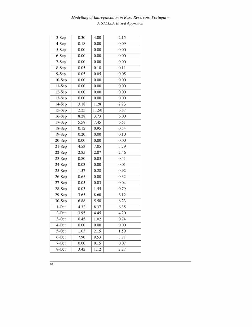
Modelling of Eutrophication in Roxo Reservoir, Portugal –
A STELLA Based Approach
66
3-Sep 0.30 4.00 2.15
4-Sep 0.18 0.00 0.09
5-Sep 0.00 0.00 0.00
6-Sep 0.00 0.00 0.00
7-Sep 0.00 0.00 0.00
8-Sep 0.05 0.18 0.11
9-Sep 0.05 0.05 0.05
10-Sep 0.00 0.00 0.00
11-Sep 0.00 0.00 0.00
12-Sep 0.00 0.00 0.00
13-Sep 0.00 0.00 0.00
14-Sep 3.18 1.28 2.23
15-Sep 2.25 11.50 6.87
16-Sep 8.28 3.73 6.00
17-Sep 5.58 7.45 6.51
18-Sep 0.12 0.95 0.54
19-Sep 0.20 0.00 0.10
20-Sep 0.00 0.00 0.00
21-Sep 4.53 7.05 5.79
22-Sep 2.85 2.07 2.46
23-Sep 0.80 0.03 0.41
24-Sep 0.03 0.00 0.01
25-Sep 1.57 0.28 0.92
26-Sep 0.65 0.00 0.32
27-Sep 0.05 0.03 0.04
28-Sep 0.03 1.55 0.79
29-Sep 3.65 8.60 6.12
30-Sep 6.88 5.58 6.23
1-Oct 4.32 8.37 6.35
2-Oct 3.95 4.45 4.20
3-Oct 0.45 1.02 0.74
4-Oct 0.00 0.00 0.00
5-Oct 1.03 2.15 1.59
6-Oct 7.90 9.53 8.71
7-Oct 0.00 0.15 0.07
8-Oct 3.42 1.12 2.27

Modelling of Eutrophication in Roxo Reservoir, Alentejo, Portugal -
A System Dynamic Based Approach
67
9-Oct 0.83 0.50 0.66
10-Oct 1.13 1.87 1.50
11-Oct 2.45 4.50 3.47
12-Oct 0.30 1.00 0.65
13-Oct 0.00 0.33 0.16
14-Oct 0.00 0.05 0.03
15-Oct 1.50 2.10 1.80
16-Oct 0.40 0.60 0.50
17-Oct 0.48 1.28 0.88
18-Oct 5.58 6.37 5.97
19-Oct 4.62 10.00 7.31
20-Oct 10.25 9.80 10.02
21-Oct 2.65 1.78 2.21
22-Oct 1.53 3.78 2.65
23-Oct 0.17 0.05 0.11
24-Oct 2.77 1.05 1.91
25-Oct 14.87 18.82 16.85
26-Oct 0.43 0.05 0.24
27-Oct 14.57 11.77 13.17
28-Oct 4.90 2.10 3.50
29-Oct 1.87 1.10 1.48
30-Oct 1.27 1.10 1.18
31-Oct 11.47 8.15 9.81
1-Nov 0.03 0.03 0.03
2-Nov 0.03 0.05 0.04
3-Nov 2.85 2.20 2.53
4-Nov 0.00 0.05 0.03
5-Nov 1.42 3.55 2.49
6-Nov 2.58 4.23 3.40
7-Nov 0.03 0.03 0.03
8-Nov 0.08 0.05 0.06
9-Nov 1.18 2.27 1.72
10-Nov 0.80 0.13 0.46
11-Nov 0.05 0.05 0.05
12-Nov 0.15 0.08 0.11
13-Nov 2.63 3.25 2.94
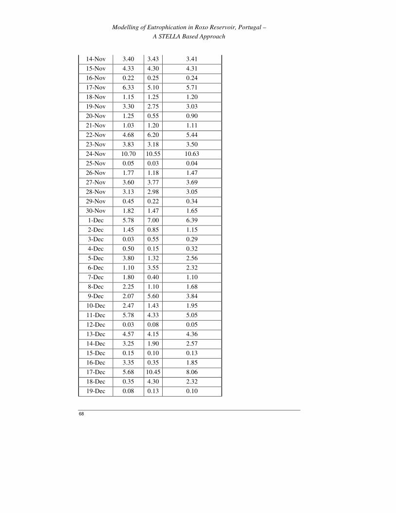
Modelling of Eutrophication in Roxo Reservoir, Portugal –
A STELLA Based Approach
68
14-Nov 3.40 3.43 3.41
15-Nov 4.33 4.30 4.31
16-Nov 0.22 0.25 0.24
17-Nov 6.33 5.10 5.71
18-Nov 1.15 1.25 1.20
19-Nov 3.30 2.75 3.03
20-Nov 1.25 0.55 0.90
21-Nov 1.03 1.20 1.11
22-Nov 4.68 6.20 5.44
23-Nov 3.83 3.18 3.50
24-Nov 10.70 10.55 10.63
25-Nov 0.05 0.03 0.04
26-Nov 1.77 1.18 1.47
27-Nov 3.60 3.77 3.69
28-Nov 3.13 2.98 3.05
29-Nov 0.45 0.22 0.34
30-Nov 1.82 1.47 1.65
1-Dec 5.78 7.00 6.39
2-Dec 1.45 0.85 1.15
3-Dec 0.03 0.55 0.29
4-Dec 0.50 0.15 0.32
5-Dec 3.80 1.32 2.56
6-Dec 1.10 3.55 2.32
7-Dec 1.80 0.40 1.10
8-Dec 2.25 1.10 1.68
9-Dec 2.07 5.60 3.84
10-Dec 2.47 1.43 1.95
11-Dec 5.78 4.33 5.05
12-Dec 0.03 0.08 0.05
13-Dec 4.57 4.15 4.36
14-Dec 3.25 1.90 2.57
15-Dec 0.15 0.10 0.13
16-Dec 3.35 0.35 1.85
17-Dec 5.68 10.45 8.06
18-Dec 0.35 4.30 2.32
19-Dec 0.08 0.13 0.10

Modelling of Eutrophication in Roxo Reservoir, Alentejo, Portugal -
A System Dynamic Based Approach
69
20-Dec 0.13 0.05 0.09
21-Dec 0.00 0.05 0.03
22-Dec 0.40 0.40 0.40
23-Dec 5.88 7.05 6.46
24-Dec 1.68 0.20 0.94
25-Dec 1.03 2.30 1.66
26-Dec 0.80 0.00 0.40
27-Dec 4.00 4.75 4.37
28-Dec 0.03 0.50 0.26
29-Dec 0.00 0.03 0.01
30-Dec 0.53 0.62 0.57
31-Dec 0.18 0.22 0.20
Source: COTR, Portugal

Modelling of Eutrophication in Roxo Reservoir, Portugal –
A STELLA Based Approach
70
Annex 2: Average Daily Light Intensity (Radiation)
Day Average Light
from Aljustrel
Station
(KJ/Day m2)
Average Light
from Beja
Station
(KJ/Day m2)
Average
Light
(KJ/day m2)
Average
Light
(KJ/s m2)
Average
Light
(W/m2)
1-Jan 2793.60 4415.22 3604.41 0.04 41.72
2-Jan 4673.90 6223.51 5448.71 0.06 63.06
3-Jan 8311.85 9617.84 8964.85 0.10 103.76
4-Jan 8908.78 10809.78 9859.28 0.11 114.11
5-Jan 8309.60 9579.16 8944.38 0.10 103.52
6-Jan 9363.45 9915.18 9639.32 0.11 111.57
7-Jan 6447.43 7556.78 7002.10 0.08 81.04
8-Jan 7407.73 8382.10 7894.91 0.09 91.38
9-Jan 7150.93 8188.03 7669.48 0.09 88.77
10-Jan 9687.58 11021.54 10354.56 0.12 119.84
11-Jan 8730.73 9983.34 9357.03 0.11 108.30
12-Jan 7956.05 11080.28 9518.17 0.11 110.16
13-Jan 7960.85 9396.85 8678.85 0.10 100.45
14-Jan 8487.83 9755.14 9121.48 0.11 105.57
15-Jan 6665.05 8196.00 7430.52 0.09 86.00
16-Jan 8928.75 9910.56 9419.66 0.11 109.02
17-Jan 7129.98 9279.93 8204.95 0.09 94.96
18-Jan 9067.83 11297.73 10182.78 0.12 117.86
19-Jan 9742.65 11814.63 10778.64 0.12 124.75
20-Jan 9235.10 10671.85 9953.48 0.12 115.20
21-Jan 9392.03 10403.45 9897.74 0.11 114.56
22-Jan 7067.50 7692.45 7379.98 0.09 85.42
23-Jan 7540.40 10662.58 9101.49 0.11 105.34
24-Jan 9035.65 10989.25 10012.45 0.12 115.88
25-Jan 8192.98 9394.55 8793.76 0.10 101.78
26-Jan 9374.98 10437.65 9906.31 0.11 114.66
27-Jan 9912.50 11290.83 10601.66 0.12 122.70
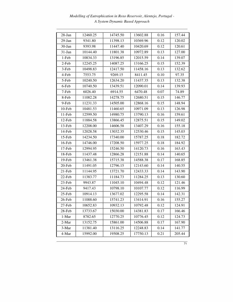
Modelling of Eutrophication in Roxo Reservoir, Alentejo, Portugal -
A System Dynamic Based Approach
71
28-Jan 12460.25 14745.50 13602.88 0.16 157.44
29-Jan 9341.80 11398.13 10369.96 0.12 120.02
30-Jan 9393.98 11447.40 10420.69 0.12 120.61
31-Jan 10144.40 11801.38 10972.89 0.13 127.00
1-Feb 10834.33 13196.85 12015.59 0.14 139.07
2-Feb 12245.25 14087.25 13166.25 0.15 152.39
3-Feb 10498.83 12417.50 11458.16 0.13 132.62
4-Feb 7553.75 9269.15 8411.45 0.10 97.35
5-Feb 10240.50 12634.20 11437.35 0.13 132.38
6-Feb 10740.50 13439.51 12090.01 0.14 139.93
7-Feb 6026.40 6914.55 6470.48 0.07 74.89
8-Feb 11082.28 14278.75 12680.51 0.15 146.77
9-Feb 11231.33 14505.00 12868.16 0.15 148.94
10-Feb 10481.53 11460.65 10971.09 0.13 126.98
11-Feb 12599.50 14980.75 13790.13 0.16 159.61
12-Feb 11884.58 13866.45 12875.51 0.15 149.02
13-Feb 12208.00 14606.58 13407.29 0.16 155.18
14-Feb 12028.58 13032.35 12530.46 0.15 145.03
15-Feb 14234.50 17340.00 15787.25 0.18 182.72
16-Feb 14746.00 17208.50 15977.25 0.18 184.92
17-Feb 12994.95 15246.50 14120.73 0.16 163.43
18-Feb 11437.48 12866.28 12151.88 0.14 140.65
19-Feb 13461.38 15715.38 14588.38 0.17 168.85
20-Feb 11491.05 12796.15 12143.60 0.14 140.55
21-Feb 11144.95 13721.70 12433.33 0.14 143.90
22-Feb 11383.77 11184.73 11284.25 0.13 130.60
23-Feb 9943.87 11045.10 10494.48 0.12 121.46
24-Feb 9417.43 10798.10 10107.77 0.12 116.99
25-Feb 10914.13 13677.02 12295.58 0.14 142.31
26-Feb 11088.60 15741.23 13414.91 0.16 155.27
27-Feb 10652.83 10932.13 10792.48 0.12 124.91
28-Feb 13733.67 15030.00 14381.83 0.17 166.46
1-Mar 8782.65 12770.25 10776.45 0.12 124.73
2-Mar 13152.75 15861.00 14506.88 0.17 167.90
3-Mar 11381.40 13116.25 12248.83 0.14 141.77
4-Mar 15992.00 19508.25 17750.13 0.21 205.44

Modelling of Eutrophication in Roxo Reservoir, Portugal –
A STELLA Based Approach
72
5-Mar 15999.50 18754.75 17377.13 0.20 201.12
6-Mar 15132.73 18009.13 16570.93 0.19 191.79
7-Mar 14307.75 17525.25 15916.50 0.18 184.22
8-Mar 17165.00 20836.75 19000.88 0.22 219.92
9-Mar 13845.75 16802.75 15324.25 0.18 177.36
10-Mar 12907.28 15454.35 14180.81 0.16 164.13
11-Mar 13015.40 15014.08 14014.74 0.16 162.21
12-Mar 10345.15 13335.15 11840.15 0.14 137.04
13-Mar 13008.63 16351.75 14680.19 0.17 169.91
14-Mar 15716.00 18247.25 16981.63 0.20 196.55
15-Mar 16075.58 19119.75 17597.66 0.20 203.68
16-Mar 15215.00 18055.00 16635.00 0.19 192.53
17-Mar 10372.42 12427.10 11399.76 0.13 131.94
18-Mar 13641.00 17453.00 15547.00 0.18 179.94
19-Mar 16116.50 17650.75 16883.63 0.20 195.41
20-Mar 18304.75 22189.75 20247.25 0.23 234.34
21-Mar 16815.08 20609.75 18712.41 0.22 216.58
22-Mar 19025.75 22751.50 20888.63 0.24 241.77
23-Mar 15570.38 17848.45 16709.41 0.19 193.40
24-Mar 15762.25 20338.50 18050.38 0.21 208.92
25-Mar 17468.00 18937.00 18202.50 0.21 210.68
26-Mar 16928.00 19546.25 18237.13 0.21 211.08
27-Mar 13371.10 14963.00 14167.05 0.16 163.97
28-Mar 10970.98 12789.15 11880.06 0.14 137.50
29-Mar 15385.25 17904.50 16644.88 0.19 192.65
30-Mar 14894.50 18287.50 16591.00 0.19 192.03
31-Mar 18377.50 22049.00 20213.25 0.23 233.95
1-Apr 14160.50 16913.50 15537.00 0.18 179.83
2-Apr 16248.00 19459.00 17853.50 0.21 206.64
3-Apr 19039.00 22422.50 20730.75 0.24 239.94
4-Apr 17198.28 20009.00 18603.64 0.22 215.32
5-Apr 18681.00 22813.00 20747.00 0.24 240.13
6-Apr 19826.75 23243.75 21535.25 0.25 249.25
7-Apr 19267.75 22821.75 21044.75 0.24 243.57
8-Apr 17908.25 17782.25 17845.25 0.21 206.54
9-Apr 18415.00 22416.00 20415.50 0.24 236.29

Modelling of Eutrophication in Roxo Reservoir, Alentejo, Portugal -
A System Dynamic Based Approach
73
10-Apr 20786.50 24226.75 22506.63 0.26 260.49
11-Apr 21381.00 23840.75 22610.88 0.26 261.70
12-Apr 18547.25 21424.00 19985.63 0.23 231.32
13-Apr 18021.88 20677.08 19349.48 0.22 223.95
14-Apr 16621.20 21562.25 19091.73 0.22 220.97
15-Apr 20241.00 23647.25 21944.13 0.25 253.98
16-Apr 21435.23 25007.97 23221.60 0.27 268.77
17-Apr 19315.39 22514.75 20915.07 0.24 242.07
18-Apr 10922.03 17227.25 14074.64 0.16 162.90
19-Apr 18296.25 22525.75 20411.00 0.24 236.24
20-Apr 20313.50 22903.50 21608.50 0.25 250.10
21-Apr 21700.75 26586.25 24143.50 0.28 279.44
22-Apr 22304.50 24625.00 23464.75 0.27 271.58
23-Apr 22323.00 26172.50 24247.75 0.28 280.65
24-Apr 22055.75 26104.00 24079.88 0.28 278.70
25-Apr 24253.25 29477.25 26865.25 0.31 310.94
26-Apr 24801.75 29787.00 27294.38 0.32 315.91
27-Apr 24944.00 29645.25 27294.63 0.32 315.91
28-Apr 19032.75 22732.00 20882.38 0.24 241.69
29-Apr 21674.25 25161.00 23417.63 0.27 271.04
30-Apr 23317.00 27260.75 25288.88 0.29 292.70
1-May 18267.75 21738.75 20003.25 0.23 231.52
2-May 17585.23 20501.85 19043.54 0.22 220.41
3-May 23383.75 27617.25 25500.50 0.30 295.14
4-May 21674.50 26001.50 23838.00 0.28 275.90
5-May 18214.50 19622.00 18918.25 0.22 218.96
6-May 23321.00 25427.50 24374.25 0.28 282.11
7-May 19456.00 22833.00 21144.50 0.24 244.73
8-May 21056.08 23780.08 22418.08 0.26 259.47
9-May 17016.75 19704.00 18360.38 0.21 212.50
10-May 20116.50 25167.25 22641.88 0.26 262.06
11-May 17009.08 20835.00 18922.04 0.22 219.01
12-May 24605.50 28979.50 26792.50 0.31 310.10
13-May 22221.50 25360.50 23791.00 0.28 275.36
14-May 26850.00 32280.50 29565.25 0.34 342.19
15-May 25494.50 29804.00 27649.25 0.32 320.01

Modelling of Eutrophication in Roxo Reservoir, Portugal –
A STELLA Based Approach
74
16-May 24724.75 28502.50 26613.63 0.31 308.03
17-May 26924.00 31613.25 29268.63 0.34 338.76
18-May 26974.00 30848.41 28911.21 0.33 334.62
19-May 27429.50 31498.52 29464.01 0.34 341.02
20-May 25205.00 29489.25 27347.13 0.32 316.52
21-May 22201.50 25879.50 24040.50 0.28 278.25
22-May 23013.75 26826.25 24920.00 0.29 288.43
23-May 24801.00 28795.00 26798.00 0.31 310.16
24-May 24410.00 30634.50 27522.25 0.32 318.54
25-May 25824.25 30336.25 28080.25 0.33 325.00
26-May 27591.25 32151.75 29871.50 0.35 345.73
27-May 26506.50 32595.25 29550.88 0.34 342.02
28-May 26161.50 30835.25 28498.38 0.33 329.84
29-May 20536.75 24664.50 22600.63 0.26 261.58
30-May 20055.25 24513.50 22284.38 0.26 257.92
31-May 25531.25 28190.78 26861.02 0.31 310.89
1-Jun 26873.25 31260.50 29066.88 0.34 336.42
2-Jun 26916.00 31102.50 29009.25 0.34 335.76
3-Jun 25360.50 28607.50 26984.00 0.31 312.31
4-Jun 22556.25 26351.50 24453.88 0.28 283.03
5-Jun 28391.00 32639.50 30515.25 0.35 353.19
6-Jun 23662.25 28064.25 25863.25 0.30 299.34
7-Jun 25408.75 29579.00 27493.88 0.32 318.22
8-Jun 25822.00 28925.00 27373.50 0.32 316.82
9-Jun 28139.50 32464.50 30302.00 0.35 350.72
10-Jun 27803.75 32098.25 29951.00 0.35 346.66
11-Jun 26935.00 30378.50 28656.75 0.33 331.68
12-Jun 25119.75 30192.25 27656.00 0.32 320.09
13-Jun 22432.50 26900.50 24666.50 0.29 285.49
14-Jun 25655.00 30448.25 28051.63 0.32 324.67
15-Jun 27834.00 32681.50 30257.75 0.35 350.21
16-Jun 24808.00 27714.00 26261.00 0.30 303.95
17-Jun 27157.25 31573.75 29365.50 0.34 339.88
18-Jun 27497.25 32293.25 29895.25 0.35 346.01
19-Jun 25011.75 30567.25 27789.50 0.32 321.64
20-Jun 27221.00 32042.25 29631.63 0.34 342.96

Modelling of Eutrophication in Roxo Reservoir, Alentejo, Portugal -
A System Dynamic Based Approach
75
21-Jun 25895.25 30792.75 28344.00 0.33 328.06
22-Jun 25667.00 29864.75 27765.88 0.32 321.36
23-Jun 26029.50 31680.50 28855.00 0.33 333.97
24-Jun 25672.75 29315.25 27494.00 0.32 318.22
25-Jun 25960.25 29361.00 27660.63 0.32 320.15
26-Jun 27644.25 32045.56 29844.90 0.35 345.43
27-Jun 27013.00 31368.75 29190.88 0.34 337.86
28-Jun 27478.50 25880.83 26679.66 0.31 308.79
29-Jun 25185.75 30457.50 27821.63 0.32 322.01
30-Jun 25082.50 29683.75 27383.13 0.32 316.93
1-Jul 28254.75 32515.50 30385.13 0.35 351.68
2-Jul 25921.50 29883.25 27902.38 0.32 322.94
3-Jul 28590.75 33204.50 30897.63 0.36 357.61
4-Jul 28639.75 33354.75 30997.25 0.36 358.76
5-Jul 28588.75 33321.25 30955.00 0.36 358.28
6-Jul 28053.50 32304.50 30179.00 0.35 349.29
7-Jul 27704.50 31891.75 29798.13 0.34 344.89
8-Jul 27745.00 32999.00 30372.00 0.35 351.53
9-Jul 27419.75 32483.75 29951.75 0.35 346.66
10-Jul 25379.75 30519.25 27949.50 0.32 323.49
11-Jul 27645.50 32314.25 29979.88 0.35 346.99
12-Jul 26374.25 31991.75 29183.00 0.34 337.77
13-Jul 22401.50 27999.75 25200.63 0.29 291.67
14-Jul 24823.75 30039.00 27431.38 0.32 317.49
15-Jul 27381.25 31301.00 29341.13 0.34 339.60
16-Jul 27793.50 32798.25 30295.88 0.35 350.65
17-Jul 27508.50 32291.25 29899.88 0.35 346.06
18-Jul 27822.25 32830.75 30326.50 0.35 351.00
19-Jul 27718.00 32507.25 30112.63 0.35 348.53
20-Jul 26053.00 30504.00 28278.50 0.33 327.30
21-Jul 26502.00 31660.75 29081.38 0.34 336.59
22-Jul 23739.75 20834.95 22287.35 0.26 257.96
23-Jul 24834.25 29882.50 27358.38 0.32 316.65
24-Jul 25529.25 30231.75 27880.50 0.32 322.69
25-Jul 24543.00 29733.25 27138.13 0.31 314.10
26-Jul 25090.00 30028.75 27559.38 0.32 318.97

Modelling of Eutrophication in Roxo Reservoir, Portugal –
A STELLA Based Approach
76
27-Jul 23237.75 27055.50 25146.63 0.29 291.05
28-Jul 26150.25 30182.25 28166.25 0.33 326.00
29-Jul 27174.50 31617.25 29395.88 0.34 340.23
30-Jul 25656.25 30254.25 27955.25 0.32 323.56
31-Jul 26344.75 30815.50 28580.13 0.33 330.79
1-Aug 26051.25 30109.50 28080.38 0.33 325.00
2-Aug 24866.25 29632.75 27249.50 0.32 315.39
3-Aug 24402.50 29364.25 26883.38 0.31 311.15
4-Aug 25660.25 30482.75 28071.50 0.32 324.90
5-Aug 21985.00 26728.50 24356.75 0.28 281.91
6-Aug 25594.00 29921.50 27757.75 0.32 321.27
7-Aug 23261.25 27492.25 25376.75 0.29 293.71
8-Aug 23114.00 26824.00 24969.00 0.29 288.99
9-Aug 19232.50 21911.75 20572.13 0.24 238.10
10-Aug 17972.00 20987.25 19479.63 0.23 225.46
11-Aug 23429.75 26876.75 25153.25 0.29 291.13
12-Aug 24396.25 28642.75 26519.50 0.31 306.94
13-Aug 24734.50 29200.00 26967.25 0.31 312.12
14-Aug 23876.25 27122.25 25499.25 0.30 295.13
15-Aug 24959.75 28688.50 26824.13 0.31 310.46
16-Aug 22543.75 25449.00 23996.38 0.28 277.74
17-Aug 23610.50 27271.00 25440.75 0.29 294.45
18-Aug 21107.25 27578.50 24342.88 0.28 281.75
19-Aug 20534.75 24890.75 22712.75 0.26 262.88
20-Aug 24480.75 28873.75 26677.25 0.31 308.76
21-Aug 23619.75 27750.25 25685.00 0.30 297.28
22-Aug 22909.25 27335.50 25122.38 0.29 290.77
23-Aug 20809.25 25197.25 23003.25 0.27 266.24
24-Aug 20624.25 22606.25 21615.25 0.25 250.18
25-Aug 21781.00 23118.38 22449.69 0.26 259.83
26-Aug 22167.75 25469.08 23818.42 0.28 275.68
27-Aug 20994.75 22539.74 21767.24 0.25 251.94
28-Aug 21592.50 22825.93 22209.21 0.26 257.05
29-Aug 22397.00 25352.23 23874.61 0.28 276.33
30-Aug 22200.75 26135.00 24167.88 0.28 279.72
31-Aug 21772.00 25906.25 23839.13 0.28 275.92

Modelling of Eutrophication in Roxo Reservoir, Alentejo, Portugal -
A System Dynamic Based Approach
77
1-Sep 18461.75 22896.75 20679.25 0.24 239.34
2-Sep 18071.08 21708.50 19889.79 0.23 230.21
3-Sep 18318.75 21426.75 19872.75 0.23 230.01
4-Sep 19474.25 24156.00 21815.13 0.25 252.49
5-Sep 21502.50 25726.50 23614.50 0.27 273.32
6-Sep 18297.00 21897.75 20097.38 0.23 232.61
7-Sep 20615.25 25180.75 22898.00 0.27 265.02
8-Sep 18484.25 21855.75 20170.00 0.23 233.45
9-Sep 20988.25 24748.75 22868.50 0.26 264.68
10-Sep 21208.75 25860.00 23534.38 0.27 272.39
11-Sep 21120.25 25752.75 23436.50 0.27 271.26
12-Sep 18365.75 23940.50 21153.13 0.24 244.83
13-Sep 19030.25 22954.00 20992.13 0.24 242.96
14-Sep 15162.60 17829.65 16496.13 0.19 190.93
15-Sep 16590.35 19775.85 18183.10 0.21 210.45
16-Sep 17665.00 21016.50 19340.75 0.22 223.85
17-Sep 17914.25 20894.33 19404.29 0.22 224.59
18-Sep 18244.50 21249.25 19746.88 0.23 228.55
19-Sep 17439.25 21137.50 19288.38 0.22 223.25
20-Sep 16735.50 19825.50 18280.50 0.21 211.58
21-Sep 14016.85 17566.63 15791.74 0.18 182.77
22-Sep 14428.13 17239.75 15833.94 0.18 183.26
23-Sep 17569.25 18982.50 18275.88 0.21 211.53
24-Sep 15204.25 16294.11 15749.18 0.18 182.28
25-Sep 15180.65 18862.41 17021.53 0.20 197.01
26-Sep 15875.75 19936.00 17905.88 0.21 207.24
27-Sep 14554.00 18478.00 16516.00 0.19 191.16
28-Sep 14006.50 18469.50 16238.00 0.19 187.94
29-Sep 13765.00 15909.08 14837.04 0.17 171.72
30-Sep 11732.83 13922.60 12827.71 0.15 148.47
1-Oct 12739.85 14532.70 13636.28 0.16 157.83
2-Oct 12515.63 16006.75 14261.19 0.17 165.06
3-Oct 13478.50 16201.50 14840.00 0.17 171.76
4-Oct 17134.25 20517.50 18825.88 0.22 217.89
5-Oct 12955.50 16494.33 14724.91 0.17 170.43
6-Oct 12003.75 14603.25 13303.50 0.15 153.98

Modelling of Eutrophication in Roxo Reservoir, Portugal –
A STELLA Based Approach
78
7-Oct 14670.33 17723.50 16196.91 0.19 187.46
8-Oct 12386.33 15192.00 13789.16 0.16 159.60
9-Oct 13903.25 16137.00 15020.13 0.17 173.84
10-Oct 11238.48 14790.75 13014.61 0.15 150.63
11-Oct 10531.65 13288.25 11909.95 0.14 137.85
12-Oct 11224.13 13837.08 12530.60 0.15 145.03
13-Oct 12292.90 13425.90 12859.40 0.15 148.84
14-Oct 12925.50 16327.25 14626.38 0.17 169.29
15-Oct 9649.78 13001.52 11325.65 0.13 131.08
16-Oct 9778.11 12882.31 11330.21 0.13 131.14
17-Oct 10446.20 13510.25 11978.23 0.14 138.64
18-Oct 7870.05 10657.70 9263.88 0.11 107.22
19-Oct 9802.38 11811.28 10806.83 0.13 125.08
20-Oct 10252.83 12445.25 11349.04 0.13 131.35
21-Oct 9801.33 12346.33 11073.83 0.13 128.17
22-Oct 12657.83 14068.45 13363.14 0.15 154.67
23-Oct 14469.00 16558.75 15513.88 0.18 179.56
24-Oct 11989.93 15531.75 13760.84 0.16 159.27
25-Oct 7566.23 9362.18 8464.20 0.10 97.97
26-Oct 10863.67 15201.75 13032.71 0.15 150.84
27-Oct 9091.80 10324.20 9708.00 0.11 112.36
28-Oct 11570.17 12582.88 12076.52 0.14 139.77
29-Oct 10923.10 11092.38 11007.74 0.13 127.40
30-Oct 9188.93 10863.85 10026.39 0.12 116.05
31-Oct 9031.30 11550.00 10290.65 0.12 119.10
1-Nov 10842.38 14299.50 12570.94 0.15 145.50
2-Nov 9951.25 12626.25 11288.75 0.13 130.66
3-Nov 6602.70 8158.35 7380.53 0.09 85.42
4-Nov 8500.23 9273.15 8886.69 0.10 102.86
5-Nov 8723.60 10217.30 9470.45 0.11 109.61
6-Nov 11358.00 13928.50 12643.25 0.15 146.33
7-Nov 11445.33 13217.75 12331.54 0.14 142.73
8-Nov 11112.58 13608.75 12360.66 0.14 143.06
9-Nov 8762.43 10401.08 9581.75 0.11 110.90
10-Nov 10628.13 13083.63 11855.88 0.14 137.22
11-Nov 10988.45 12742.13 11865.29 0.14 137.33

Modelling of Eutrophication in Roxo Reservoir, Alentejo, Portugal -
A System Dynamic Based Approach
79
12-Nov 10727.83 12965.00 11846.41 0.14 137.11
13-Nov 8967.25 10582.75 9775.00 0.11 113.14
14-Nov 9232.40 11095.60 10164.00 0.12 117.64
15-Nov 9191.35 11437.95 10314.65 0.12 119.38
16-Nov 10063.65 12045.88 11054.76 0.13 127.95
17-Nov 8740.00 10387.53 9563.76 0.11 110.69
18-Nov 9020.03 11379.73 10199.88 0.12 118.05
19-Nov 8313.55 10556.65 9435.10 0.11 109.20
20-Nov 8424.95 11294.70 9859.83 0.11 114.12
21-Nov 7590.10 9479.23 8534.66 0.10 98.78
22-Nov 8202.63 9412.05 8807.34 0.10 101.94
23-Nov 8436.18 10342.48 9389.33 0.11 108.67
24-Nov 7215.38 8551.90 7883.64 0.09 91.25
25-Nov 10394.75 12410.50 11402.63 0.13 131.97
26-Nov 7405.85 9302.80 8354.33 0.10 96.69
27-Nov 5304.63 6954.58 6129.60 0.07 70.94
28-Nov 6253.20 8123.98 7188.59 0.08 83.20
29-Nov 6001.95 7402.93 6702.44 0.08 77.57
30-Nov 5784.50 8217.20 7000.85 0.08 81.03
1-Dec 5681.85 7396.43 6539.14 0.08 75.68
2-Dec 8776.73 9986.88 9381.80 0.11 108.59
3-Dec 7033.73 8725.23 7879.48 0.09 91.20
4-Dec 5744.53 8738.70 7241.61 0.08 83.81
5-Dec 7080.93 9584.98 8332.95 0.10 96.45
6-Dec 8592.65 9628.45 9110.55 0.11 105.45
7-Dec 8732.68 10390.08 9561.38 0.11 110.66
8-Dec 7122.80 8842.90 7982.85 0.09 92.39
9-Dec 6549.33 7830.35 7189.84 0.08 83.22
10-Dec 7482.00 9155.18 8318.59 0.10 96.28
11-Dec 6445.18 7543.83 6994.50 0.08 80.95
12-Dec 6848.45 8048.80 7448.63 0.09 86.21
13-Dec 4495.20 5660.65 5077.93 0.06 58.77
14-Dec 7212.98 8119.00 7665.99 0.09 88.73
15-Dec 8290.13 10168.95 9229.54 0.11 106.82
16-Dec 5972.90 7674.45 6823.68 0.08 78.98
17-Dec 4077.15 4502.05 4289.60 0.05 49.65

Modelling of Eutrophication in Roxo Reservoir, Portugal –
A STELLA Based Approach
80
18-Dec 5615.45 6787.59 6201.52 0.07 71.78
19-Dec 7483.43 8695.12 8089.27 0.09 93.63
20-Dec 7093.90 8176.28 7635.09 0.09 88.37
21-Dec 7390.90 9432.38 8411.64 0.10 97.36
22-Dec 8324.10 9183.66 8753.88 0.10 101.32
23-Dec 7517.08 8331.66 7924.37 0.09 91.72
24-Dec 8580.10 10115.86 9347.98 0.11 108.19
25-Dec 6903.95 8120.33 7512.14 0.09 86.95
26-Dec 7404.05 9418.99 8411.52 0.10 97.36
27-Dec 7194.48 8935.27 8064.87 0.09 93.34
28-Dec 8077.75 9958.08 9017.91 0.10 104.37
29-Dec 7172.58 8563.45 7868.01 0.09 91.06
30-Dec 6571.25 8043.19 7307.22 0.08 84.57
31-Dec 6077.60 7145.73 6611.66 0.08 76.52
Source: COTR, Portugal

Modelling of Eutrophication in Roxo Reservoir, Alentejo, Portugal -
A System Dynamic Based Approach
81
Annex3: Average Daily Temperature
Day
Average Daily
Temperature
from Beja Station
(ºC)
Average Daily
Temperature from
Aljustrel Station
(ºC)
Average Daily
Temperature
(ºC)
1-Jan 9.62 11.92 10.77
2-Jan 9.74 11.76 10.75
3-Jan 8.52 10.13 9.33
4-Jan 7.40 8.99 8.20
5-Jan 7.90 9.83 8.86
6-Jan 6.74 8.66 7.70
7-Jan 6.80 9.31 8.05
8-Jan 7.41 9.72 8.56
9-Jan 7.71 9.81 8.76
10-Jan 6.14 8.76 7.45
11-Jan 6.18 8.31 7.24
12-Jan 6.22 8.04 7.13
13-Jan 6.61 8.84 7.72
14-Jan 6.84 9.04 7.94
15-Jan 6.51 8.90 7.70
16-Jan 6.34 8.43 7.38
17-Jan 6.67 8.69 7.68
18-Jan 7.23 9.22 8.23
19-Jan 6.85 8.99 7.92
20-Jan 7.38 9.14 8.26
21-Jan 6.94 9.33 8.14
22-Jan 7.25 9.80 8.53
23-Jan 7.87 9.44 8.65
24-Jan 8.11 9.29 8.70
25-Jan 8.06 9.38 8.72
26-Jan 9.26 10.18 9.72
27-Jan 10.85 10.66 10.76

Modelling of Eutrophication in Roxo Reservoir, Portugal –
A STELLA Based Approach
82
28-Jan 9.19 9.25 9.22
29-Jan 7.39 8.34 7.86
30-Jan 7.93 9.21 8.57
31-Jan 8.13 9.06 8.60
1-Feb 7.63 8.76 8.19
2-Feb 8.22 10.13 9.18
3-Feb 8.60 10.55 9.58
4-Feb 8.90 10.59 9.74
5-Feb 9.15 10.83 9.99
6-Feb 7.97 9.79 8.88
7-Feb 7.94 9.62 8.78
8-Feb 8.13 9.86 9.00
9-Feb 8.04 10.25 9.14
10-Feb 8.61 10.75 9.68
11-Feb 9.33 11.57 10.45
12-Feb 8.81 10.84 9.83
13-Feb 7.89 9.97 8.93
14-Feb 6.67 9.24 7.96
15-Feb 6.23 8.53 7.38
16-Feb 6.48 8.26 7.37
17-Feb 7.24 8.62 7.93
18-Feb 7.87 9.92 8.89
19-Feb 5.92 9.05 7.49
20-Feb 6.42 8.48 7.45
21-Feb 7.22 9.40 8.31
22-Feb 8.66 11.03 9.85
23-Feb 9.40 11.20 10.30
24-Feb 7.88 11.45 9.66
25-Feb 7.33 10.12 8.72
26-Feb 6.64 9.64 8.14
27-Feb 7.00 10.11 8.56
28-Feb 8.18 10.73 9.46
1-Mar 7.24 9.23 8.23
2-Mar 7.06 9.56 8.31
3-Mar 7.99 10.11 9.05
4-Mar 9.01 10.54 9.77

Modelling of Eutrophication in Roxo Reservoir, Alentejo, Portugal -
A System Dynamic Based Approach
83
5-Mar 8.65 10.46 9.56
6-Mar 8.28 10.84 9.56
7-Mar 8.13 10.79 9.46
8-Mar 9.52 11.73 10.63
9-Mar 8.85 11.41 10.13
10-Mar 9.92 12.10 11.01
11-Mar 10.31 13.96 12.14
12-Mar 10.24 13.75 11.99
13-Mar 9.18 13.05 11.11
14-Mar 8.69 12.57 10.63
15-Mar 9.50 13.04 11.27
16-Mar 9.53 13.81 11.67
17-Mar 8.69 13.49 11.09
18-Mar 9.82 14.14 11.98
19-Mar 10.23 14.49 12.36
20-Mar 11.14 15.63 13.39
21-Mar 10.95 15.20 13.07
22-Mar 11.46 15.34 13.40
23-Mar 11.25 14.78 13.02
24-Mar 11.13 14.78 12.95
25-Mar 10.54 15.36 12.95
26-Mar 9.89 14.24 12.06
27-Mar 9.44 13.62 11.53
28-Mar 8.93 13.07 11.00
29-Mar 9.68 13.97 11.83
30-Mar 9.54 14.34 11.94
31-Mar 10.10 15.85 12.98
1-Apr 10.18 15.12 12.65
2-Apr 9.21 13.23 11.22
3-Apr 9.13 13.44 11.29
4-Apr 9.53 13.79 11.66
5-Apr 11.18 15.31 13.25
6-Apr 10.57 14.86 12.71
7-Apr 10.13 14.38 12.26
8-Apr 10.41 14.12 12.26
9-Apr 9.95 13.34 11.65

Modelling of Eutrophication in Roxo Reservoir, Portugal –
A STELLA Based Approach
84
10-Apr 9.02 12.76 10.89
11-Apr 8.43 12.56 10.49
12-Apr 9.62 13.97 11.80
13-Apr 9.81 14.32 12.06
14-Apr 9.59 13.26 11.43
15-Apr 10.43 13.83 12.13
16-Apr 9.68 12.98 11.33
17-Apr 9.59 13.46 11.53
18-Apr 9.42 13.33 11.38
19-Apr 9.52 13.24 11.38
20-Apr 11.18 14.84 13.01
21-Apr 11.94 15.88 13.91
22-Apr 11.38 15.89 13.64
23-Apr 12.21 16.39 14.30
24-Apr 13.94 17.58 15.76
25-Apr 14.32 18.09 16.20
26-Apr 13.16 17.86 15.51
27-Apr 13.52 18.15 15.84
28-Apr 11.44 16.96 14.20
29-Apr 11.01 16.41 13.71
30-Apr 10.66 15.75 13.20
1-May 10.20 15.04 12.62
2-May 9.40 14.40 11.90
3-May 10.71 15.64 13.17
4-May 11.31 16.51 13.91
5-May 10.46 16.64 13.55
6-May 10.50 16.91 13.71
7-May 9.47 15.41 12.44
8-May 10.27 15.60 12.94
9-May 10.90 15.87 13.38
10-May 10.81 16.09 13.45
11-May 10.76 15.73 13.25
12-May 12.32 17.00 14.66
13-May 12.88 17.21 15.04
14-May 14.88 18.90 16.89
15-May 15.23 19.23 17.23

Modelling of Eutrophication in Roxo Reservoir, Alentejo, Portugal -
A System Dynamic Based Approach
85
16-May 14.14 18.09 16.12
17-May 13.59 18.13 15.86
18-May 13.96 19.21 16.58
19-May 15.13 21.03 18.08
20-May 14.23 19.42 16.82
21-May 14.83 20.05 17.44
22-May 14.68 19.27 16.98
23-May 14.22 19.27 16.75
24-May 13.01 18.72 15.87
25-May 13.28 19.18 16.23
26-May 13.31 19.34 16.32
27-May 13.99 19.16 16.58
28-May 14.87 20.00 17.43
29-May 16.16 21.14 18.65
30-May 15.90 20.81 18.35
31-May 17.35 22.28 19.81
1-Jun 16.21 22.48 19.34
2-Jun 15.88 21.73 18.80
3-Jun 15.27 20.73 18.00
4-Jun 14.14 20.57 17.36
5-Jun 13.90 20.73 17.31
6-Jun 14.56 21.71 18.14
7-Jun 15.57 22.75 19.16
8-Jun 15.47 22.53 19.00
9-Jun 16.10 22.18 19.14
10-Jun 17.45 23.24 20.35
11-Jun 19.30 24.37 21.84
12-Jun 19.99 24.41 22.20
13-Jun 19.07 23.85 21.46
14-Jun 18.35 22.88 20.61
15-Jun 17.47 22.73 20.10
16-Jun 17.37 24.23 20.80
17-Jun 18.38 25.37 21.88
18-Jun 18.30 24.58 21.44
19-Jun 17.93 24.49 21.21
20-Jun 17.15 24.43 20.79

Modelling of Eutrophication in Roxo Reservoir, Portugal –
A STELLA Based Approach
86
21-Jun 17.49 24.88 21.18
22-Jun 16.97 24.06 20.51
23-Jun 16.52 22.24 19.38
24-Jun 15.92 21.67 18.79
25-Jun 16.98 22.06 19.52
26-Jun 15.91 22.38 19.15
27-Jun 18.06 22.91 20.49
28-Jun 19.02 23.22 21.12
29-Jun 17.47 22.42 19.94
30-Jun 16.30 21.84 19.07
1-Jul 16.46 22.60 19.53
2-Jul 16.40 23.04 19.72
3-Jul 16.84 22.87 19.86
4-Jul 17.06 22.74 19.90
5-Jul 16.93 23.08 20.01
6-Jul 15.94 22.79 19.37
7-Jul 16.36 21.96 19.16
8-Jul 16.36 22.46 19.41
9-Jul 16.69 23.25 19.97
10-Jul 17.10 23.66 20.38
11-Jul 16.99 23.48 20.23
12-Jul 17.20 23.54 20.37
13-Jul 17.74 23.05 20.39
14-Jul 18.41 23.77 21.09
15-Jul 17.88 23.52 20.70
16-Jul 17.94 22.78 20.36
17-Jul 18.35 23.48 20.91
18-Jul 18.40 23.68 21.04
19-Jul 17.83 23.89 20.86
20-Jul 16.86 23.75 20.30
21-Jul 16.48 22.01 19.24
22-Jul 17.40 22.35 19.88
23-Jul 18.69 24.22 21.46
24-Jul 20.72 25.75 23.23
25-Jul 20.96 26.06 23.51
26-Jul 20.34 25.74 23.04

Modelling of Eutrophication in Roxo Reservoir, Alentejo, Portugal -
A System Dynamic Based Approach
87
27-Jul 19.39 24.83 22.11
28-Jul 18.65 23.88 21.27
29-Jul 19.25 23.98 21.61
30-Jul 19.72 24.71 22.22
31-Jul 20.53 25.47 23.00
1-Aug 20.99 25.33 23.16
2-Aug 19.52 25.53 22.52
3-Aug 18.12 24.82 21.47
4-Aug 18.38 25.47 21.93
5-Aug 19.18 26.14 22.66
6-Aug 19.73 26.92 23.33
7-Aug 19.33 25.30 22.32
8-Aug 19.36 24.88 22.12
9-Aug 17.83 23.16 20.50
10-Aug 17.78 23.16 20.47
11-Aug 19.62 24.87 22.24
12-Aug 20.77 26.62 23.70
13-Aug 20.85 26.87 23.86
14-Aug 19.56 26.12 22.84
15-Aug 17.71 24.54 21.12
16-Aug 17.44 23.28 20.36
17-Aug 17.32 22.90 20.11
18-Aug 17.01 22.66 19.83
19-Aug 16.90 22.44 19.67
20-Aug 16.85 23.28 20.06
21-Aug 17.54 23.70 20.62
22-Aug 17.74 23.99 20.87
23-Aug 17.05 23.28 20.16
24-Aug 16.92 22.91 19.91
25-Aug 17.59 22.99 20.29
26-Aug 17.12 22.59 19.85
27-Aug 16.22 21.69 18.95
28-Aug 17.09 22.88 19.98
29-Aug 17.90 23.82 20.86
30-Aug 17.68 23.73 20.71
31-Aug 16.91 22.24 19.57

Modelling of Eutrophication in Roxo Reservoir, Portugal –
A STELLA Based Approach
88
1-Sep 21.85 21.21 21.53
2-Sep 20.73 20.73 20.73
3-Sep 21.06 21.19 21.13
4-Sep 21.78 21.51 21.65
5-Sep 20.73 20.77 20.75
6-Sep 20.69 20.67 20.68
7-Sep 21.04 20.89 20.96
8-Sep 22.04 21.99 22.02
9-Sep 22.62 22.18 22.40
10-Sep 22.70 21.74 22.22
11-Sep 23.32 23.04 23.18
12-Sep 22.91 22.81 22.86
13-Sep 21.80 21.39 21.60
14-Sep 21.35 21.10 21.23
15-Sep 21.56 21.56 21.56
16-Sep 23.28 22.95 23.12
17-Sep 23.04 22.64 22.84
18-Sep 22.01 21.83 21.92
19-Sep 21.66 21.83 21.75
20-Sep 21.51 21.26 21.39
21-Sep 21.25 21.18 21.22
22-Sep 20.74 20.71 20.72
23-Sep 20.95 21.15 21.05
24-Sep 20.72 20.02 20.37
25-Sep 20.35 20.17 20.26
26-Sep 21.32 20.89 21.10
27-Sep 21.18 20.92 21.05
28-Sep 21.26 21.30 21.28
29-Sep 20.87 21.13 21.00
30-Sep 20.23 20.25 20.24
1-Oct 19.62 19.50 19.56
2-Oct 20.78 20.32 20.55
3-Oct 21.35 20.95 21.15
4-Oct 21.14 20.71 20.92
5-Oct 20.52 20.35 20.43
6-Oct 19.72 19.82 19.77

Modelling of Eutrophication in Roxo Reservoir, Alentejo, Portugal -
A System Dynamic Based Approach
89
7-Oct 19.68 20.28 19.98
8-Oct 19.26 19.74 19.50
9-Oct 16.56 17.35 16.95
10-Oct 15.74 16.34 16.04
11-Oct 17.02 16.86 16.94
12-Oct 17.68 17.73 17.70
13-Oct 17.34 17.24 17.29
14-Oct 16.89 16.80 16.85
15-Oct 16.97 17.02 16.99
16-Oct 16.17 15.90 16.03
17-Oct 16.32 15.78 16.05
18-Oct 16.63 16.25 16.44
19-Oct 17.73 19.30 18.51
20-Oct 17.79 19.33 18.56
21-Oct 17.32 17.76 17.54
22-Oct 16.58 16.40 16.49
23-Oct 15.28 14.91 15.10
24-Oct 15.24 15.08 15.16
25-Oct 15.62 15.62 15.62
26-Oct 16.44 16.13 16.29
27-Oct 17.14 17.13 17.13
28-Oct 17.22 16.49 16.86
29-Oct 16.31 15.95 16.13
30-Oct 15.93 14.83 15.38
31-Oct 15.27 14.02 14.65
1-Nov 15.80 15.68 15.74
2-Nov 15.19 15.13 15.16
3-Nov 15.41 16.10 15.76
4-Nov 14.26 15.07 14.67
5-Nov 14.87 15.36 15.12
6-Nov 16.37 17.11 16.74
7-Nov 15.69 16.24 15.97
8-Nov 14.97 14.34 14.66
9-Nov 12.86 12.51 12.68
10-Nov 11.48 11.66 11.57
11-Nov 10.66 10.85 10.75
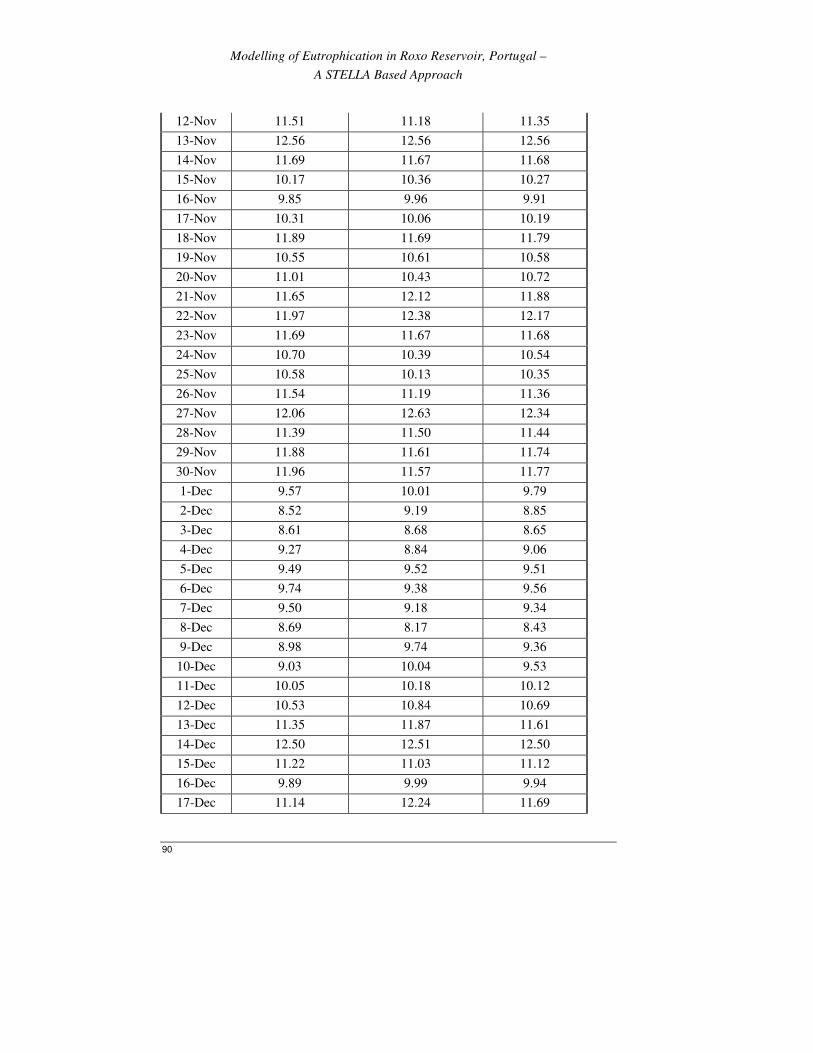
Modelling of Eutrophication in Roxo Reservoir, Portugal –
A STELLA Based Approach
90
12-Nov 11.51 11.18 11.35
13-Nov 12.56 12.56 12.56
14-Nov 11.69 11.67 11.68
15-Nov 10.17 10.36 10.27
16-Nov 9.85 9.96 9.91
17-Nov 10.31 10.06 10.19
18-Nov 11.89 11.69 11.79
19-Nov 10.55 10.61 10.58
20-Nov 11.01 10.43 10.72
21-Nov 11.65 12.12 11.88
22-Nov 11.97 12.38 12.17
23-Nov 11.69 11.67 11.68
24-Nov 10.70 10.39 10.54
25-Nov 10.58 10.13 10.35
26-Nov 11.54 11.19 11.36
27-Nov 12.06 12.63 12.34
28-Nov 11.39 11.50 11.44
29-Nov 11.88 11.61 11.74
30-Nov 11.96 11.57 11.77
1-Dec 9.57 10.01 9.79
2-Dec 8.52 9.19 8.85
3-Dec 8.61 8.68 8.65
4-Dec 9.27 8.84 9.06
5-Dec 9.49 9.52 9.51
6-Dec 9.74 9.38 9.56
7-Dec 9.50 9.18 9.34
8-Dec 8.69 8.17 8.43
9-Dec 8.98 9.74 9.36
10-Dec 9.03 10.04 9.53
11-Dec 10.05 10.18 10.12
12-Dec 10.53 10.84 10.69
13-Dec 11.35 11.87 11.61
14-Dec 12.50 12.51 12.50
15-Dec 11.22 11.03 11.12
16-Dec 9.89 9.99 9.94
17-Dec 11.14 12.24 11.69

Modelling of Eutrophication in Roxo Reservoir, Alentejo, Portugal -
A System Dynamic Based Approach
91
18-Dec 11.50 11.97 11.74
19-Dec 10.90 11.06 10.98
20-Dec 9.64 10.25 9.94
21-Dec 10.02 10.33 10.17
22-Dec 9.42 10.21 9.81
23-Dec 9.25 10.30 9.77
24-Dec 9.21 9.19 9.20
25-Dec 9.62 9.99 9.81
26-Dec 9.00 9.64 9.32
27-Dec 8.72 8.59 8.65
28-Dec 8.30 8.29 8.30
29-Dec 8.36 8.88 8.62
30-Dec 10.82 11.29 11.05
31-Dec 11.75 11.22 11.49
Source: COTR, Portugal

Modelling of Eutrophication in Roxo Reservoir, Portugal –
A STELLA Based Approach
92
Annex 4: Detail parametric chart of Model 3
Component Acronym Type Unit Initial Value Equation Source
Water Inflow WIn Flow m3/d Time Series --- 1
Water Ouflow WOut Flow m3/d Time Series --- 2
Evapotranspiration E Flow m3/d Time Series --- 2
Water in Reservoir W Stock m3/d 50000000
dWW WIn WOut E
dt= + − −
Concentration of Nitrate ConcN Controller mg/l
--- *1000
N
W
Monod constant for
Nitrate KN Controller
mg
N/l 0.01 ---
3
Ammonia Preference
Factor APF Controller ---
1.46 ---
3
Nitrate Limiting Factor NLF Controller ---
---
( * )* APF ConcAConcC e
ConcN KN
−
+
3
Nitrate Inflow NIn Flow mg/d --- *6.1*1000WIn 4
Nitrate Outflow NOut Flow mg/d --- *WOut ConcN
Nitrate Consumed NCon Flow mg/l --- * * * *TPB LLF TLF NLF MGR
3, 5
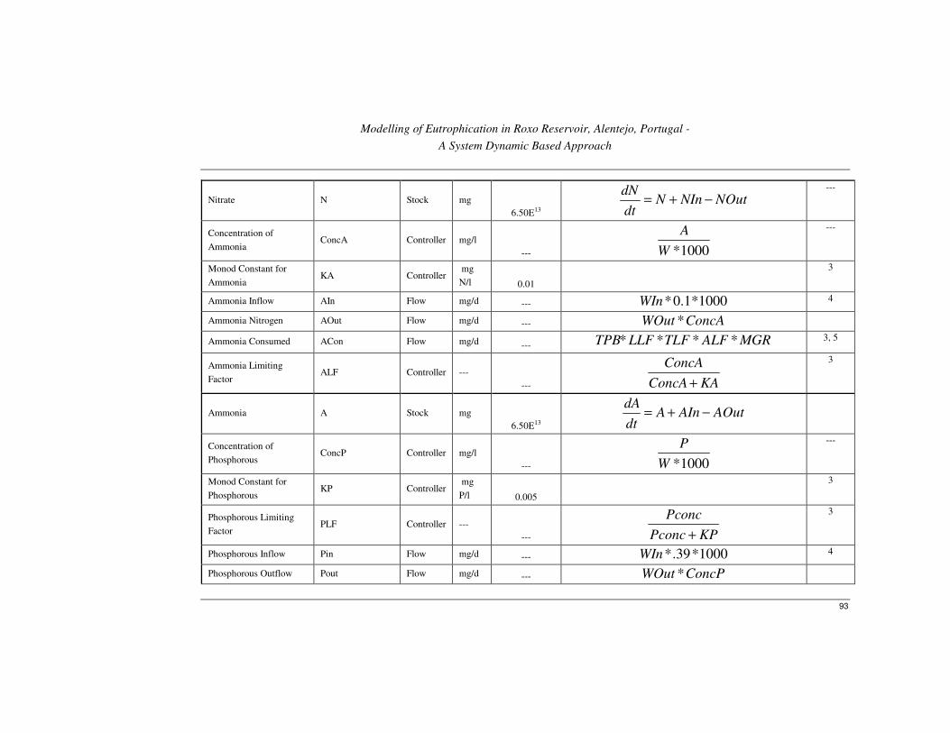
Modelling of Eutrophication in Roxo Reservoir, Alentejo, Portugal -
A System Dynamic Based Approach
93
Nitrate N Stock mg
6.50E13
dNN NIn NOut
dt= + −
---
Concentration of
Ammonia ConcA Controller mg/l
--- *1000
A
W
---
Monod Constant for
Ammonia KA Controller
mg
N/l 0.01
3
Ammonia Inflow AIn Flow mg/d --- *0.1*1000WIn 4
Ammonia Nitrogen AOut Flow mg/d --- *WOut ConcA
Ammonia Consumed ACon Flow mg/d --- * * * *TPB LLF TLF ALF MGR
3, 5
Ammonia Limiting
Factor ALF Controller ---
---
ConcA
ConcA KA+
3
Ammonia A Stock mg
6.50E13
dAA AIn AOut
dt= + −
Concentration of
Phosphorous ConcP Controller mg/l
--- *1000
P
W
---
Monod Constant for
Phosphorous KP Controller
mg
P/l 0.005
3
Phosphorous Limiting
Factor PLF Controller ---
---
Pconc
Pconc KP+
3
Phosphorous Inflow Pin Flow mg/d --- *.39*1000WIn 4
Phosphorous Outflow Pout Flow mg/d --- *WOut ConcP

Modelling of Eutrophication in Roxo Reservoir, Portugal –
A STELLA Based Approach
94
Phosphorous Consumed PC Flow mg/d --- * * * *TPB LLF TLF PLF MGR
3, 5
Phosphorous P Stock mg
8.00E11
dPP PIn POut
dt= + −
Nutrient Limiting Factor NuLF Controller --- --- [ , ( )]Min PLF NLF ALF+
3, 5
Light Intensity LI Controller W/m2 Time Series --- 1
Optimal Light Intensity OLI Controller W/m2 250 --- 3
Light Limiting Factor LLF Controller ---
---
(1)*
LIOLILI e
OLI
−
6
Temperature T Controller º C Time Series --- 1
Optimal Temperature OT Controller º C 23 --- 5
Low Lethal Temperature Lt Controller º C 5 ---
5
Xt -- Controller ---
---
T OTXt
OT Lt
−=
−
5
Shape Factor for
Temperature Limiting
Factor
SF Controller ---
-0.7 ---
5
Temperature Limiting
Factor TLF Controller ---
--- 2
2*(1 )*
( 2* * 1)
SF XtTLF
Xt SF Xt
+=
+ +
5
Maximum Growth Rate MGR Controller --- 0.9 --- 3, 5, 7
Graxing Rate GR Controller 0.265 --- 8
Death Rate DR Controller 0.3 --- 8

Modelling of Eutrophication in Roxo Reservoir, Alentejo, Portugal -
A System Dynamic Based Approach
95
Respiration Rate
Constant RRC Controller
0.1 ---
3
Temperature Constant
for Respiration TCR Controller ---
1 ---
3
Nutrient Accessibility
Inhibition Coefficient of
Cyanobacteria
NAInCoeffCyano Controller ---
2*10-11 ---
8
Nutrient Accessibility
Inhibition Coefficient of
C. hirundinela
NAINCoeffChiru Controller ---
1.8*10-11 ---
8
Percentage of Nutrient
Available for C.
hirundinela
PNAviChiru Controller ---
--- *NuLF Cyano NAINCoeffCyano−
8
C. hirundinela Growth ChiruGrowth Flow mg/d --- * * * *Chiru MGR LLF TLF ANAviChiru 3, 5
C. hirundinela Death ChiruDeath Flow mg/d --- ( 20)*[ ( * ) ]T
Chiru DR TCR RRC GR−
+ +
3, 5
C. hirundinela Biomass Chiru Stock mg
812500000
dChiruChiru ChiruGrowth ChiruDeath
dt= + −
3, 5
Toxicity Coefficient ToxCoeff Controller 5.5*10-3 --- 8
Percentage of Nutirent
Available to
Cyanobacteria
PNAviCyano Controller ---
--- *NuLF Chiru NAINCoeffChiru−
8
Cyanobacteria Growth CyanoGrowth Flow mg/d --- * * * *Cyano MGR LLF TLF ANAviCyano
3, 5
Cyanobacteria Death CyanoDeath Flow mg/d --- ( 20)*[ ( * ) ] *T
Cyano DR TCR RRC GR Chiru ToxCoeff−
+ + + 3, 5
Cyanobacteria Biomass Cyano Stock mg 812500000
dCyanoCyano CyanoGrowth CyanoDeath
dt= + −
3, 5

Modelling of Eutrophication in Roxo Reservoir, Portugal –
A STELLA Based Approach
96
Total Phytoplankton
Biomass TPB Controller mg
--- ( )Chiru Cyano+
Chlorophyll-a Pigment ChP Controller µg/µg
0.4 ---
9
Chlorophyll-a Ch Controller µg --- *( *1000)ChP TPB
---
Chlorophyll-a
Concentration ChConc Controller µg/l
--- ( *1000)
Ch
W
---
1: CORT, Portugal
2: Woldie, 2003
3: ITC, 2000
4: EMAS, Portugal
5: Beckers, et al., 1999
6: Pelletier, 1999
7: Strom, et al., 1999
8: Assumed value
9: Felip, et al., 2000
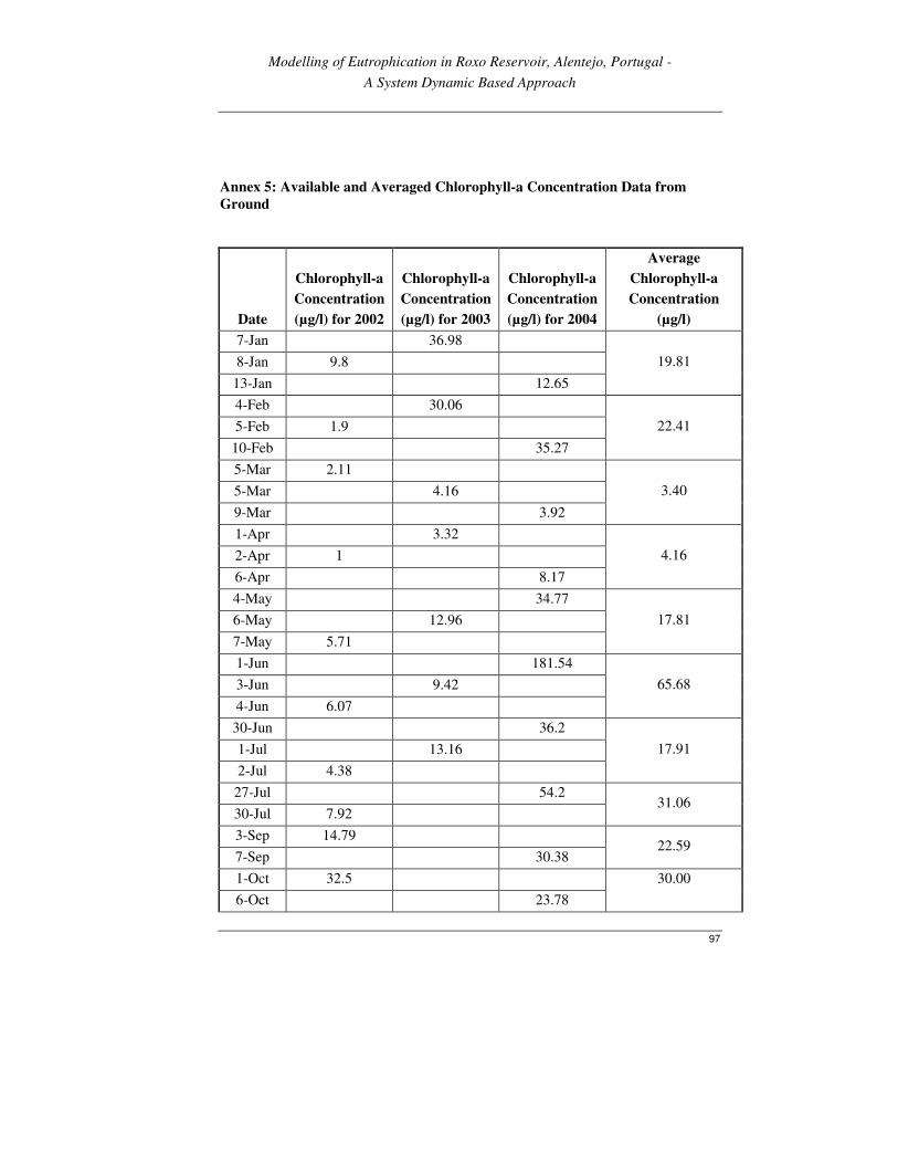
Modelling of Eutrophication in Roxo Reservoir, Alentejo, Portugal -
A System Dynamic Based Approach
97
Annex 5: Available and Averaged Chlorophyll-a Concentration Data from
Ground
Date
Chlorophyll-a
Concentration
(µg/l) for 2002
Chlorophyll-a
Concentration
(µg/l) for 2003
Chlorophyll-a
Concentration
(µg/l) for 2004
Average
Chlorophyll-a
Concentration
(µg/l)
7-Jan 36.98
8-Jan 9.8
13-Jan 12.65
19.81
4-Feb 30.06
5-Feb 1.9
10-Feb 35.27
22.41
5-Mar 2.11
5-Mar 4.16
9-Mar 3.92
3.40
1-Apr 3.32
2-Apr 1
6-Apr 8.17
4.16
4-May 34.77
6-May 12.96
7-May 5.71
17.81
1-Jun 181.54
3-Jun 9.42
4-Jun 6.07
65.68
30-Jun 36.2
1-Jul 13.16
2-Jul 4.38
17.91
27-Jul 54.2
30-Jul 7.92 31.06
3-Sep 14.79
7-Sep 30.38 22.59
1-Oct 32.5
6-Oct 23.78
30.00

Modelling of Eutrophication in Roxo Reservoir, Portugal –
A STELLA Based Approach
98
7-Oct 33.72
29-Oct 191.75
2-Nov 56.88
4-Nov 118.75
122.46
26-Nov 26.8
30-Nov 89.29
2-Dec 18.84
44.98

Modelling of Eutrophication in Roxo Reservoir, Alentejo, Portugal -
A System Dynamic Based Approach
99
Annex 6: Averaged Chlorophyll-a Concentration as Predicted by Model 3
Date
Chlorophyll-a Concentration
Predicted by Model 3 (µg/l)
Average Chlorophyll-a
Concentration (µg/l)
7-Jan 12.98
8-Jan 12.93
13-Jan 12.93
12.95
4-Feb 12.87
5-Feb 12.88
10-Feb 12.90
12.88
5-Mar 12.68
9-Mar 12.73 12.71
1-Apr 12.48
2-Apr 12.45
6-Apr 12.47
12.47
4-May 12.51
6-May 12.56
7-May 12.58
12.55
1-Jun 62.59
3-Jun 63.09
4-Jun 67.09
64.26
30-Jun 37.34
1-Jul 38.99
2-Jul 38.90
38.41
27-Jul 21.11
30-Jul 18.48 19.80
3-Sep 14.18
7-Sep 16.88 15.53
1-Oct 22.48
6-Oct 25.04
7-Oct 25.35
24.29
29-Oct 136.94
2-Nov 181.04
166.80

Modelling of Eutrophication in Roxo Reservoir, Portugal –
A STELLA Based Approach
100
4-Nov 182.43
26-Nov 0.46
30-Nov 0.07
2-Dec 0.03
0.19