Statistical Analysis – Chapter 9Regression-Correlation Pt. II

Dr. Roderick Graham

Fashion Institute of Technology

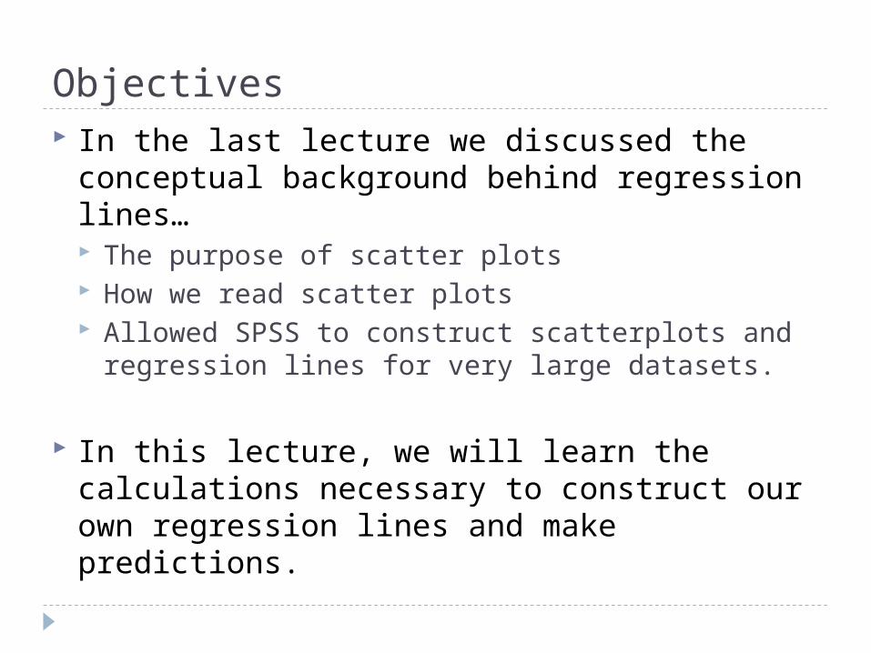
Objectives In the last lecture we discussed the

conceptual background behind regression lines… The purpose of scatter plots How we read scatter plots Allowed SPSS to construct scatterplots and

regression lines for very large datasets.

In this lecture, we will learn the calculations necessary to construct our own regression lines and make predictions.

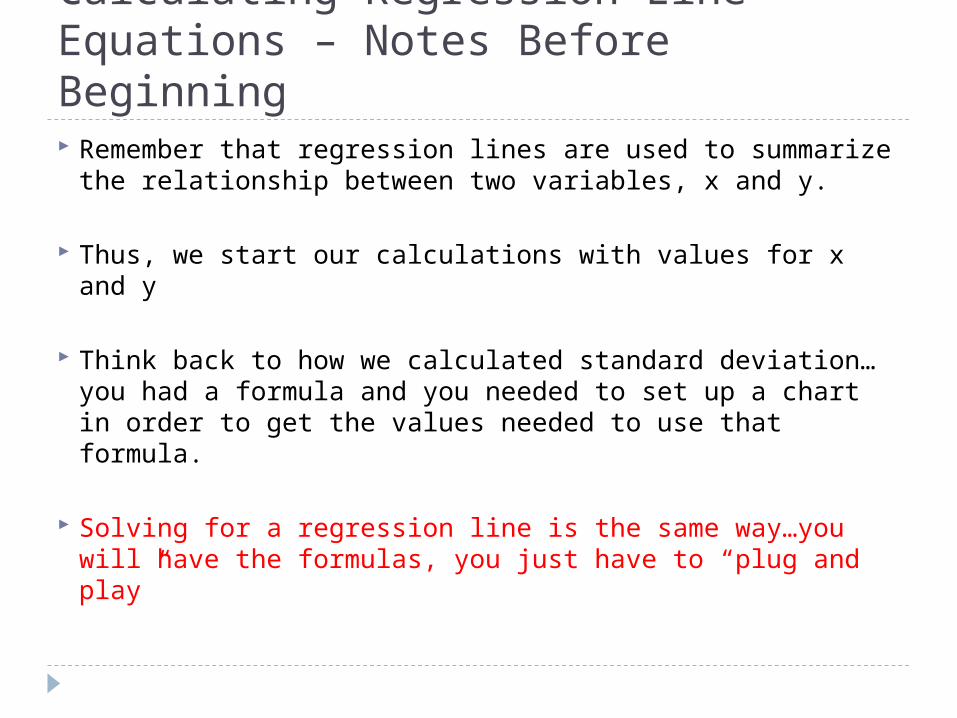
Calculating Regression Line Equations – Notes Before Beginning Remember that regression lines are used to summarize

the relationship between two variables, x and y.

Thus, we start our calculations with values for x and y

Think back to how we calculated standard deviation…you had a formula and you needed to set up a chart in order to get the values needed to use that formula.

Solving for a regression line is the same way…you will have the formulas, you just have to “plug and play”

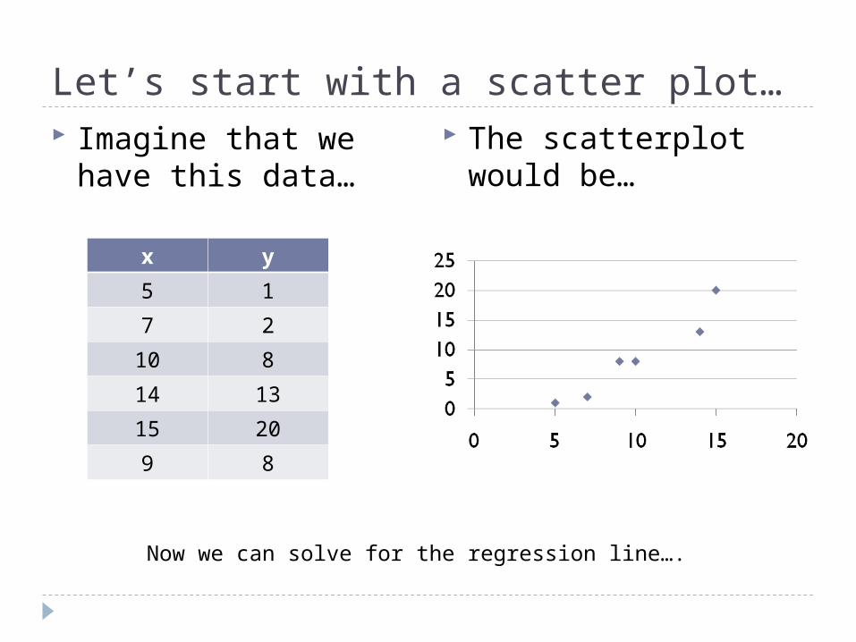
Let’s start with a scatter plot… Imagine that we

have this data… The scatterplot

would be…

x y

5 1

7 2

10 8

14 13

15 20

9 8

Now we can solve for the regression line….

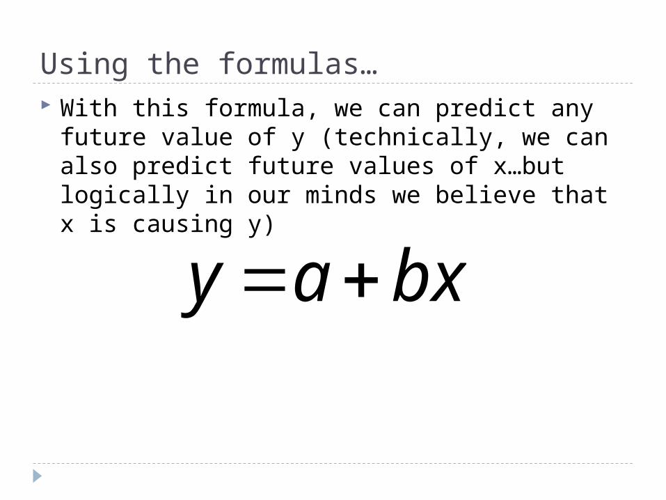
Using the formulas… With this formula, we can predict any future

value of y (technically, we can also predict future values of x…but logically in our minds we believe that x is causing y)

bxay

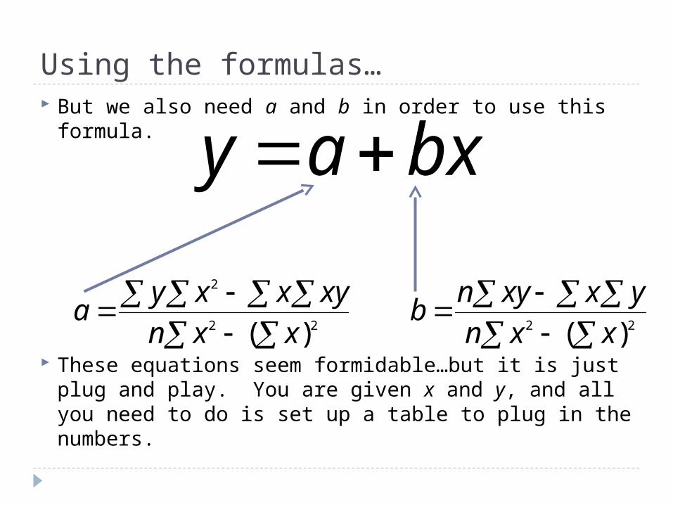
Using the formulas… But we also need a and b in order to use this

formula.

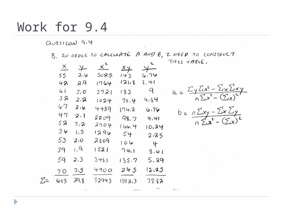
These equations seem formidable…but it is just plug and play. You are given x and y, and all you need to do is set up a table to plug in the numbers.

bxay

22

2

)( xxn

xyxxya

22 )( xxn

yxxynb

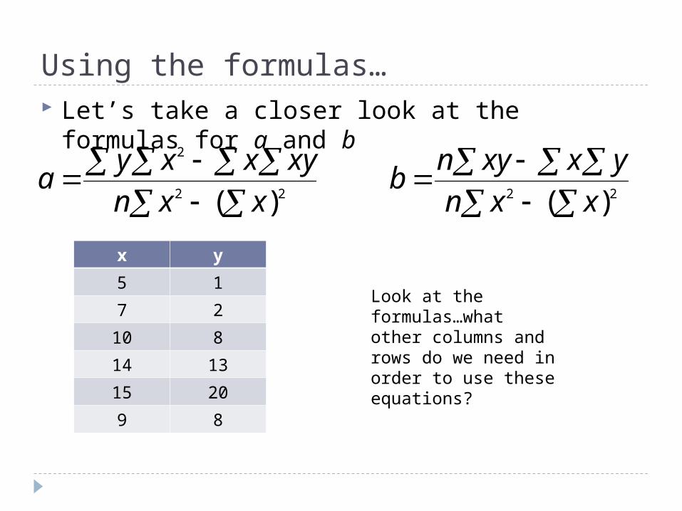
Using the formulas… Let’s take a closer look at the formulas for a

and b

22

2

)( xxn

xyxxya

22 )( xxn

yxxynb

x y

5 1

7 2

10 8

14 13

15 20

9 8

Look at the formulas…what other columns and rows do we need in order to use these equations?

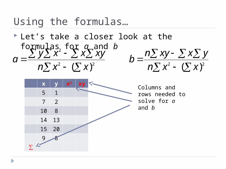
Using the formulas… Let’s take a closer look at the formulas for a

and b

22

2

)( xxn

xyxxya

22 )( xxn

yxxynb

x y x2 xy

5 1

7 2

10 8

14 13

15 20

9 8

∑

Columns and rows needed to solve for a and b

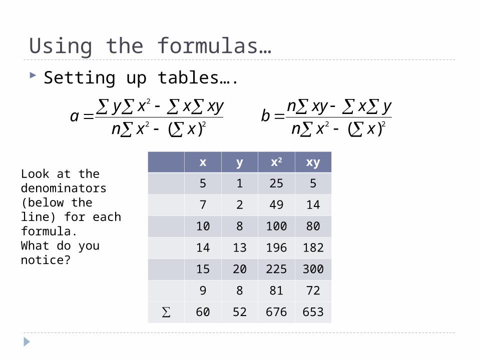
Using the formulas… Setting up tables….

22

2

)( xxn

xyxxya

22 )( xxn

yxxynb

x y x2 xy

5 1 25 5

7 2 49 14

10 8 100 80

14 13 196 182

15 20 225 300

9 8 81 72

∑ 60 52 676 653

Look at the denominators (below the line) for each formula.What do you notice?

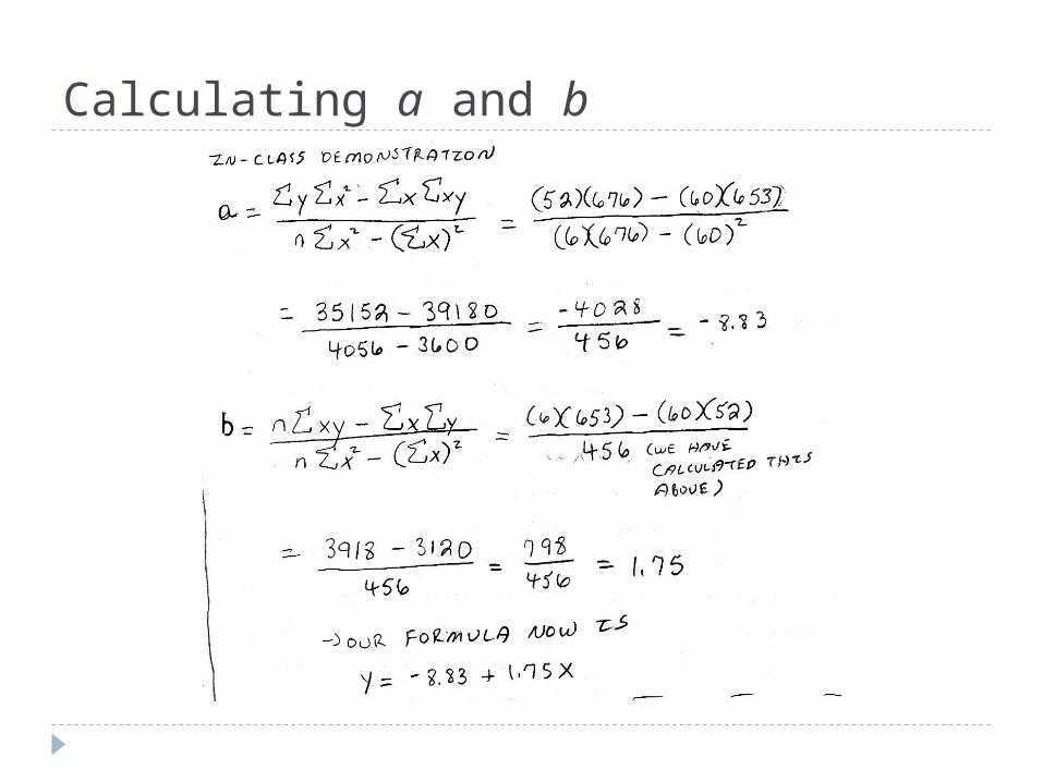
Calculating a and b

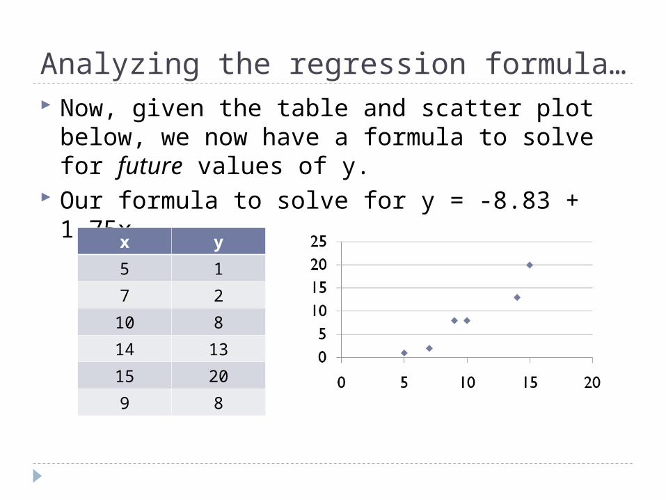
Analyzing the regression formula… Now, given the table and scatter plot below,

we now have a formula to solve for future values of y.

Our formula to solve for y = -8.83 + 1.75x

x y

5 1

7 2

10 8

14 13

15 20

9 8

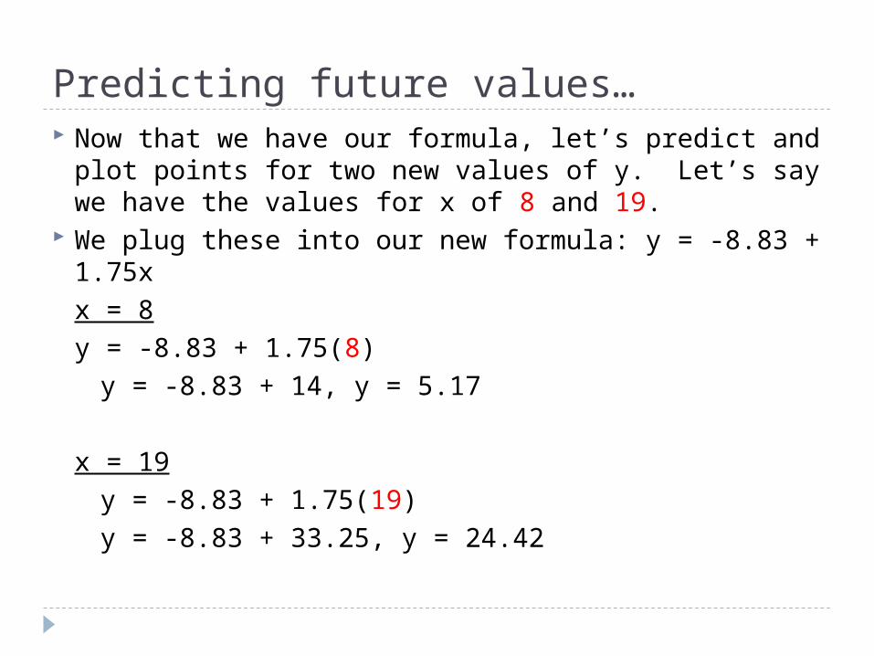
Predicting future values… Now that we have our formula, let’s predict and

plot points for two new values of y. Let’s say we have the values for x of 8 and 19.

We plug these into our new formula: y = -8.83 + 1.75xx = 8y = -8.83 + 1.75(8)

y = -8.83 + 14, y = 5.17

x = 19 y = -8.83 + 1.75(19) y = -8.83 + 33.25, y = 24.42

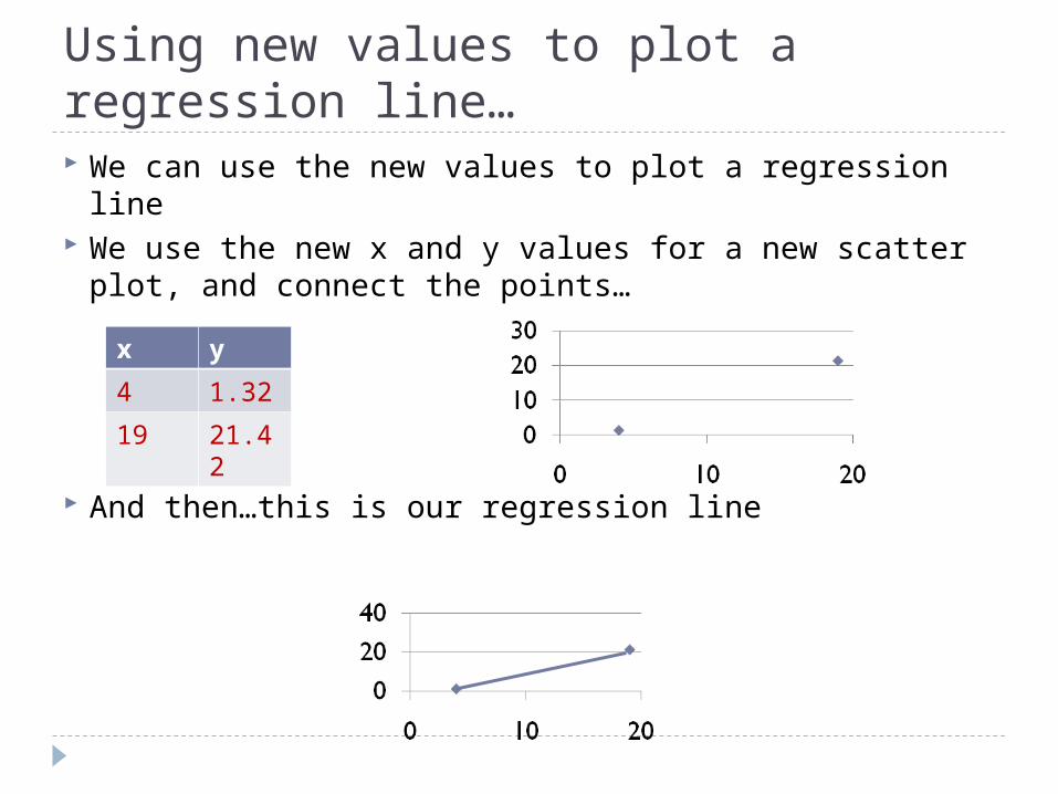
Using new values to plot a regression line… We can use the new values to plot a regression line We use the new x and y values for a new scatter

plot, and connect the points…

And then…this is our regression line

x y

4 1.32

19 21.42

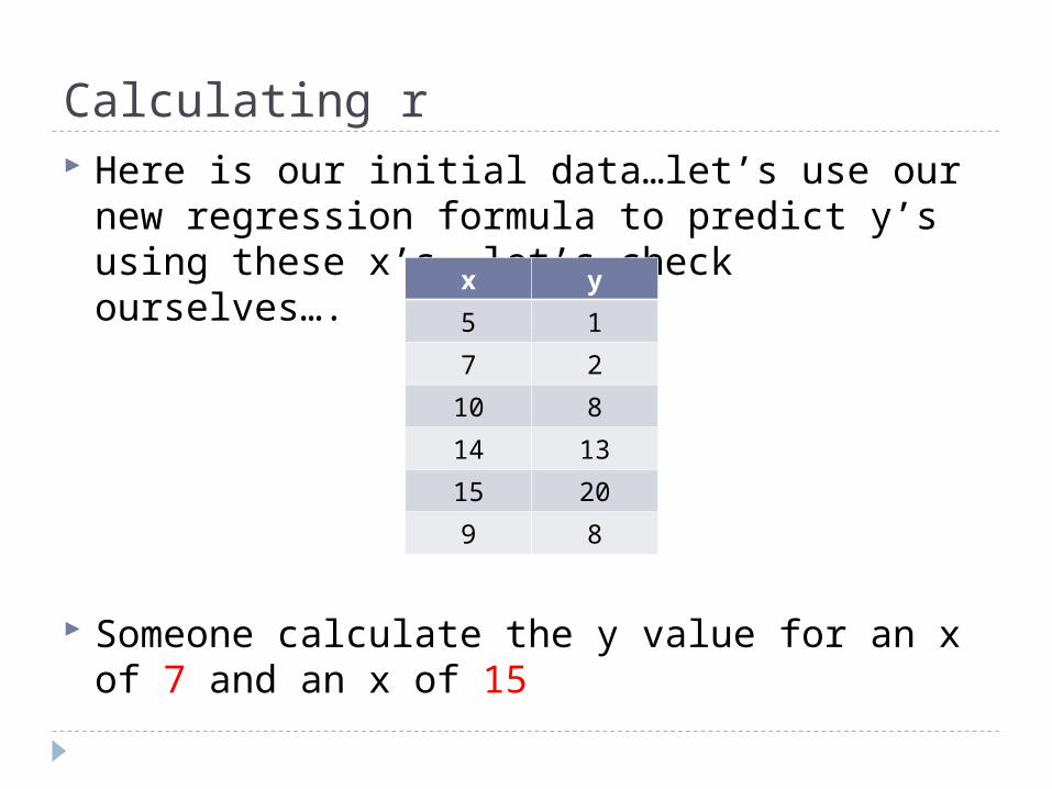
Calculating r Here is our initial data…let’s use our new

regression formula to predict y’s using these x’s….let’s check ourselves….

Someone calculate the y value for an x of 7 and an x of 15

x y

5 1

7 2

10 8

14 13

15 20

9 8

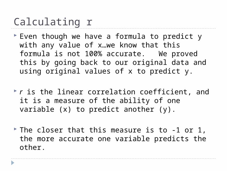
Calculating r Even though we have a formula to predict y

with any value of x…we know that this formula is not 100% accurate. We proved this by going back to our original data and using original values of x to predict y.

r is the linear correlation coefficient, and it is a measure of the ability of one variable (x) to predict another (y).

The closer that this measure is to -1 or 1, the more accurate one variable predicts the other.

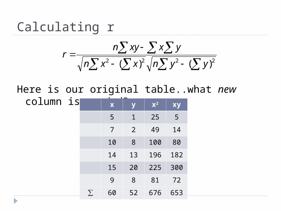
Calculating r

Here is our original table..what new column is needed? x y x2 xy

5 1 25 5

7 2 49 14

10 8 100 80

14 13 196 182

15 20 225 300

9 8 81 72

∑ 60 52 676 653

2222 )()( yynxxn

yxxynr

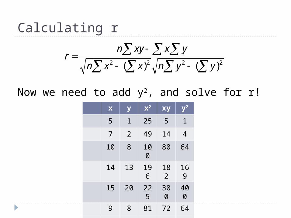
Calculating r

Now we need to add y2, and solve for r! x y x2 xy y2

5 1 25 5 1

7 2 49 14 4

10 8 100

80 64

14 13 196

182

169

15 20 225

300

400

9 8 81 72 64

∑ 60 52 676

653

702

2222 )()( yynxxn

yxxynr

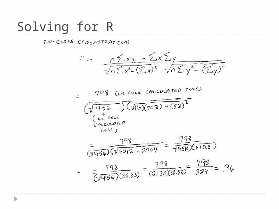
Solving for R

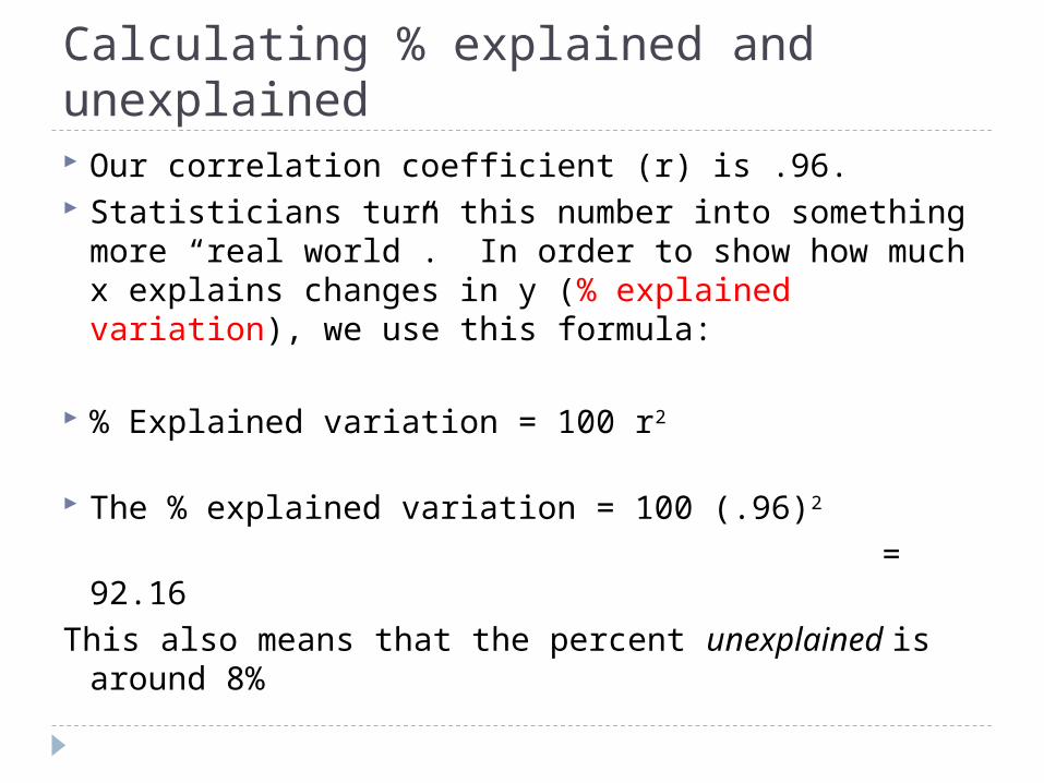
Calculating % explained and unexplained Our correlation coefficient (r) is .96. Statisticians turn this number into something

more “real world”. In order to show how much x explains changes in y (% explained variation), we use this formula:

% Explained variation = 100 r2

The % explained variation = 100 (.96)2

= 92.16This also means that the percent unexplained is

around 8%

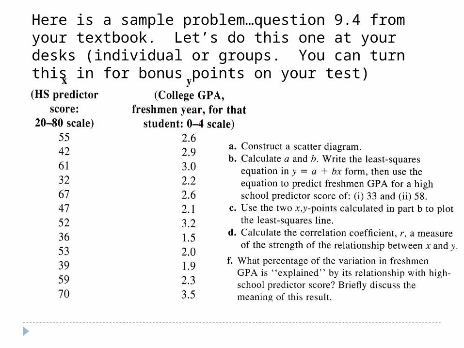
Here is a sample problem…question 9.4 from your textbook. Let’s do this one at your desks (individual or groups. You can turn this in for bonus points on your test)

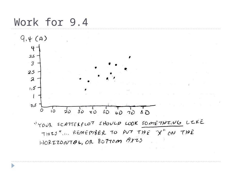
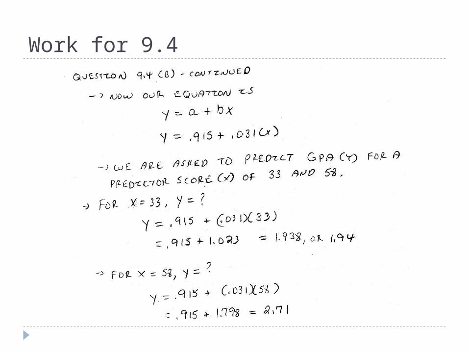
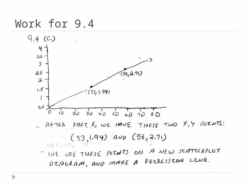
Work for 9.4

Work for 9.4

Work for 9.4

Work for 9.4

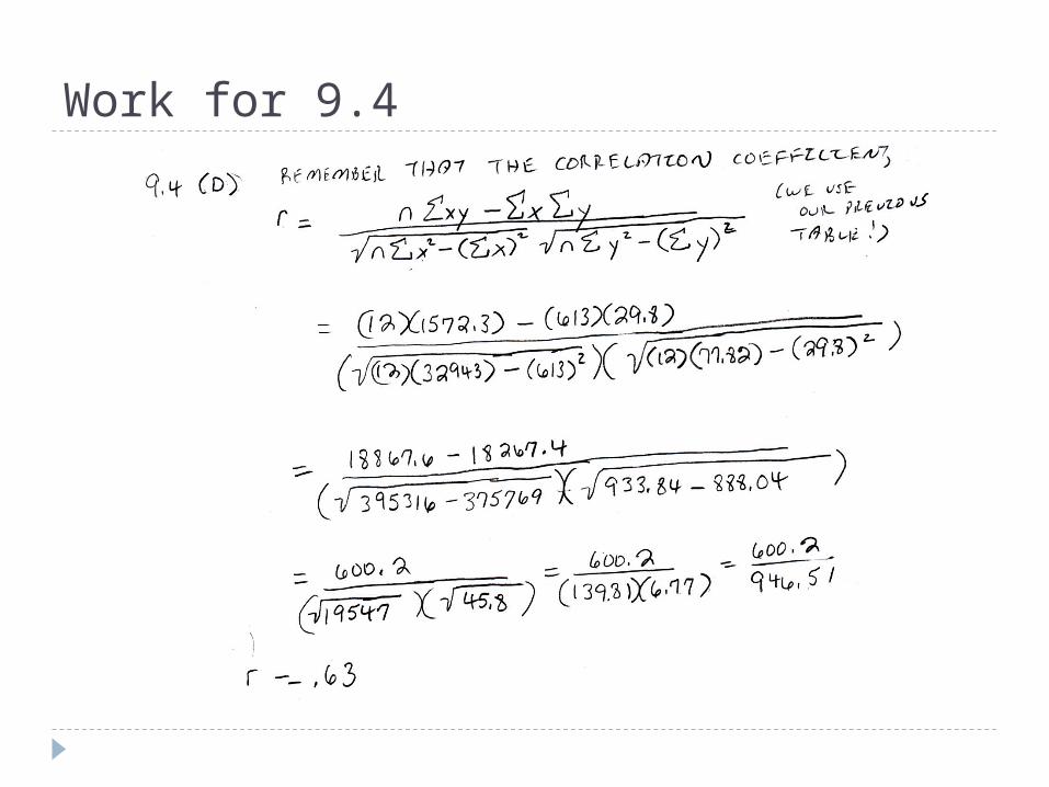
Work for 9.4

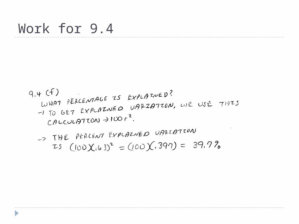
Work for 9.4

END