Statewide Network Data Analysis and Kriging Project - Final Report John Welhan, Idaho Geological Survey, Idaho State University, 208-282-4254, welhjohn@isu.edu Melissa Merrick, Idaho State University, Geosciences Department Background and Goals This project was conceived out of discussions that arose at meetings of the Ground Water Monitoring Technical Committee in late 2000 and early 2001 concerning technically defensible ways to identify temporal trends in ground water quality, specifically for prioritizing areas of management concern for nitrate contamination. Welhan suggested that spatial mapping of ground water quality monitoring data via kriging could be used to provide an optimal estimate of the spatial extent of ground-water contamination for any analyte, as well as providing a quantitative, statistical, and areally-weighted means of defining the statistical significance of apparent change. Subsequent discussions with the Idaho Department of Water Resources (IDWR) led to the creation of this project to utilize the Statewide Ground Water Quality Monitoring Network (hereafter referred to as the Statewide network) and its 12-year water quality database to evaluate the feasibility of using geostatistical methods to map spatial distributions and to quantify temporal water quality trends on the basis of statistical significance. In its essence, kriging is an optimal estimator (Isaaks and Srivastava, 1989) that can be used to synthesize water quality data collected at discrete locations (wells) into a map of the spatial pattern of water quality variations. Kriging estimates are based on available point measurements and the spatial statistical nature of the measurements; the kriging estimates are automatically tagged with an associated measure of their estimation uncertainty--the kriging variance (σ2

K). This quantity can be used to classify both the relative level of confidence of the kriged water quality maps as well as to quantify the statistical confidence level of apparent changes in water quality from one sampling period to another. The project had several broad goals: a) examining the feasibility of the kriging approach to analyze nitrate, arsenic, and selected pesticide data from the statewide network, b) mapping patterns of water quality variations (both spatial and temporal), c) demonstrating the utility of geostatistical methods for filtering and synthesis of monitoring data, and d) recommending those data analysis methods which show the greatest promise as future management tools. Project Tasks The project was designed around a two-year phased timetable with three tasks in the first phase (data analysis, method development, and mapping) and two in the second (reporting and technology transfer/training): Project Tasks: 1. Identify and map spatial/temporal trends in nitrate for specific areas as well as statewide; 2. Create maps of the probability of exceeding action thresholds for nitrate, pesticides, arsenic; 3. Evaluate relationships between pesticide and nitrate, arsenic and inorganic parameters, and evaluate the feasibility of using cokriging to improve mapping of pesticide and arsenic; 4. Prepare a final report of project methods, results, and recommendations; and

5. Provide technology transfer via worked data examples, training materials, training workshop. This report is intended to satisfy elements of Tasks 4 and 5, in conjunction with a two-day training workshop conducted in October, 2003. The report is structured around the results of the first three tasks and results and recommendations arising therefrom. Approach and Methodology Scope: The analytes of interest to IDWR were nitrate, arsenic, and pesticides. Given the plethora of different pesticides in the Statewide network's database and the fact that relatively few exceed analytical detection limits in much of the state, only atrazine was examined in detail, both statistically and geostatistically, because it is the most commonly detected pesticide, statewide, and because the number of occurrences above the analytical detection limit permitted a spatial statistical analysisin at least some areas. Temporal trends and exceedance probability for nitrate were mapped in specified areas (Twin Falls, Treasure Valley, Clearwater Plateau, as well as other areas that had sufficient data to support a geostatistical analysis), and also presented as statewide summary maps. Arsenic and atrazine exceedance probabilities were mapped only in areas having sufficient numbers of analyses above detection threshold and were also presented as statewide summary maps. Temporal trends in arsenic were mapped only in those hydrologic subareas that had sufficient numbers of measurements above detection limit. Statistical analyses for bivariate correlations and conditional expectation that could be exploited on a cokriging approach (Task 3) were performed on nitrate and atrazine as well as between arsenic and selected inorganic parameters in those hydrologic subareas having sufficient sampling information. However, so few of the relationships found were statistically significant or meaningful that the analysis could not be extended to a statewide scope or to other areas of interest (such as the Treasure Valley or Clearwater Plateau). Presentation of Results:

All mapping and geostatistical calculations were performed using ESRI Inc.'s ArcMap 8.2 GIS platform, using its Geostatistical Analyst and Spatial Analyst extensions. Considerable documentation of methods, problems, and workarounds was generated during the project. In addition, training examples were designed and included with the results to provide a level of technology transfer as required under Task 5, to allow IDWR and other users to develop in-house analytical capabilities. To streamline accessibility to project results, documentation, and training materials, a Project Reporting Interface was designed and implemented for Task 1, Task 2, and Task 3. This hyperlinked reporting format provides access to primary project documentation from a single location. All project documentation can be accessed via Explorer under the appropriate \Task1, \Task2, or \Task3 folders as well as in the \Documentation subfolders under \Nitrate, \Arsenic, or \Atrazine. The ReadME.txt file on the accompanying CD-ROM should be consulted for copying CD contents and accessing this and other documentation.

GIS mapping results are also accessed through the reporting interface, although a bug in MS Word created problems in linking to ArcGIS projects directly from the reporting interface. A workaround was found using links to intermediate shortcut files. Aside from the reporting

interface, individual GIS projects can be accessed either via Explorer or the ArcGIS statewide maps; the latter GIS maps are also hyperlinked to summaries of project results at a statewide scale. Projects used as training examples in the reporting interface can be accessed directly via Explorer. In all cases, ArcGIS's hyperlink capability is activated by clicking on the hyperlink tool (small lightning bolt) and clicking on the desired hydrologic subarea to navigate to linked projects. In those instances where multiple hydrologic subareas overlap (e.g., Treasure Valley), the appropriate ArcGIS project file must be selected from a list of possible links. The Database: IDWR provided analyte data from the Statewide Ground Water Quality Monitoring Program, as well as well locations and hydrologic subarea designations in a Microsoft Access database. The data represent all analyte information collected in the Statewide program from 1990 to 2001 (12 years) representing over 1800 monitoring wells throughout Idaho. About 400 sites are sampled annually on a rotating basis. Most sites in the database are sampled once every four years; only about 100 sites are sampled every year. The database represents three rounds of complete statewide rotational coverage: sites sampled in 1990-1994, sites sampled in 1995-1998, and a partial coverage of sites sampled in 1999-2001. Temporal change analysis could have been performed on a year-by year basis by comparing nitrate kriging estimates based on each year’s sampling data. Kriging provides an optimal estimate of water quality on the basis of nearest neighbor data points plus a measure of prediction confidence so that even measuring point locations change from year to year, kriging predictions at any specified location could still be compared to esimate temporal change. However, because the number of wells that are sampled annually in a given area of the Statewide network is usually insufficient to produce confidant kriging estimates on an annual basis, two or more years of Statewide data were composited into three time periods for kriging and temporal change analysis.

Data compositing was a trade-off between maintaining spatial data density within map subareas and minimizing the “smearing” of temporal information across annual sampling events. To avoid the introduction of spatial statistical bias due to different numbers of samples, the 1990-2001 data were segregated into three groups of roughly equal numbers of measurements representing samples collected during 1990-1993, 1994-1997, and 1998-2001. These three groupings also represent fairly similar spatial distributions of sampling locales determined by the Statewide network’s rotating sampling scheme. Maps of the statewide distribution of wells for each time period can be accessed from the ArcGIS projects from the Project Reporting Interfaces; information on specific database queries and supporting documentation can be accessed here. Exploratory Data Evaluation: Data analysis commenced with three phases of exploratory evaluation: a) general statistical characteristics, b) temporal homogeneity, and c) identification of spatial outliers. All nitrate data were found to be distributed non-normally (strongly right-skewed), although the degree of non-normality varied from year to year and from composited time period to time period. Ordinary kriging accommodates non-normally distributed data as long as spatial autocorrelation structure is not masked by extreme-valued outliers (Isaaks and Srivastava, 1989); therefore, minor differences in the shape of the distribution from time period to time period will not cause problems for temporal change analysis under most circumstances. However, if the

statistical distributions between the time periods being compared are significantly different, both accuracy and sensitivity of the temporal change analysis method could be affected. Therefore, the nitrate data were tested for temporal homogeneity between individual years and between composited time periods; in all cases, the data distributions were statistically indistinguishable at the 95% confidence level. The most significant finding at the exploratory data evaluation stage was the identification of spatial outliers in the data. In contrast to statistical (extreme-valued) outliers which may cluster in space and conform to the spatial autocorrelation structure of the overall data set, spatial outliers are anomalous because they violate the autocorrelation pattern of the data set. Such high-valued measurements, if not handled appropriately, can severely mask underlying autocorrelation structure in the data and lead to poor or inaccurate kriging estimates. The issue is especially important in comparing two time periods in which spatial outliers occur only in one time period or in different locations in the two time periods (because of sampling rotation). Fortunately, geostatistical tools can greatly facilitate our ability to identify, isolate, and deal with spatial outliers. Details on how to apply these tools are provided in the training example and documentation under the Task 1 reporting interface. All data sets that were kriged in this project were subjected to this process of spatial data filtering in which spatial outliers were identified and temporarily removed prior to variogram analysis. In all but a few of the most extreme cases these high-valued outliers were added back to the data sets prior to kriging.

The decision to exclude extreme-valued data in making spatial estimates will always be a subjective one. Whether a sampling location is chronically high-valued or if high values occur sporadically, their impact on temporal and/or spatial variability may be out of proportion to the physical relevance of the information they represent. All such situations should be examined on a case by case basis. In all cases, spatial data filtering is a cost-effective means of screening a database for anomalous values that may arise from laboratory, database, or transcriptional errors, and/or questionable sample/well integrity (e.g., casing leakage, surface contamination, etc.). Grid Representation: Kriging predictions are commonly represented in the form of contour maps, filled contour maps, or color-classified continuous change maps. However, such representations are themselves interpretations because contouring is based on a grid of interpolated values. Although grid estimates can be made on a very fine spacing, such estimates (and resulting contours) are not necessarily more accurate and can actually be less so. One of the tremendous advantages of kriging is its ability to make estimates that are optimal for either point or area-based assignments; hence, contours based on a grid of kriged estimates can be made optimal in different senses. Rather than representing the kriging results as traditional contour maps, all results have been mapped on grids. This decision was based on the need to maximize both accuracy and efficiency of the kriging process and subsequent GIS computations. The rationale is two-fold: 1. Block kriging returns estimates that are representative of and optimal for an entire

grid cell not just the grid center point, so that comparisons between sampling periods are automatically areally weighted; and

2. Spatial comparisons and calculations of temporal change are accomplished using raster arithmetic; therefore, block kriged estimates are naturally better suited to raster- based computations.

ArcGIS’s Geostatistical Analyst does not provide a block-kriging option. Instead, only point kriging estimates are returned on a very fine grid. Block kriging estimates are subsequently computed from the point estimates by converting the point-kriged estimates to a raster coverage and specifying the desired grid extents, point-averaging scheme, and block size1. We determined that a 4 x 4 point averaging scheme was more than adequate to correctly convert the point-kriged results to block estimates for these data sets. (Note: although Spatial Analyst's simplified kriging interface seems to explicitly allow for the choice between block and point kriging, it is based on the same analysis engine and the same grid averaging parameters). The block kriging cell size can be made arbitrarily fine, although too fine a grid can be computationally inefficient. Conversely, too coarse a grid can lead to bias in the block-kriged estimates. The choice of block kriging cell size is discussed in a following section. A 1.5 x 1.5 km square cell was found to be the coarsest grid that avoids bias arising from block averaging but fine enough to represent regional spatial variability (see supporting documentation). All project computations were made at this grid resolution. Task-Specific Results and Discussion

All analyses were performed on a spatial scale that utilized IDWR’s designated hydrologic unit boundaries (areas in which hydrogeological conditions are generally similar). However, it must be recognized that such hydrologic designations are quite broad and will encompass a variety of different aquifers and flow regimes within their boundaries. As such, all spatial modeling of water quality within these areas must be considered a first-order representation of the actual spatial variation of water quality in a given aquifer within that region. However, the techniques and approach documented in this report are applicable at all spatial scales; they can perform even better on a smaller scale in site-specific areas where sufficient subsurface information exists to define hydrogeologic flow regimes. In all cases, sufficient monitoring data must be available to justify a geostatitical approach (at least 30 spatially- distributed samples in the area being analyzed).

In the case of the state’s valley aquifers (e.g., Basin and Range valley areas), insufficient sample coverage in any given valley, together with a marked spatial anisotropy of sample availability (i.e., wells are distributed only up and down a valley, with no lateral coverage within a valley) required that data be composited spatially as well as temporally. On the assumption that the hydrogeologic regimes, gradients, sediment type, etc are similar among valleys, nitrate data from groups of valleys in each sampling period were analyzed as a single population with the proviso that autocorrelation structure would only be considered in a direction parallel to the axis of the valleys. Block Kriging and Optimal Cell Size All kriging was performed on discrete blocks in order to best represent average water quality conditions over discrete areas rather than individual points. This ensures that estimates are not overly sensitive to localalized high-values and are spatially representative. To ensure that 1 Although the kriging interface in ArcGIS’s Spatial Analyst appears to explicitly allow for the choice of block kriging (through a choice of cell size), it is based on the same geostatistical analysis and computation engine and uses the same grid averaging approach to rasterize point kriging output.

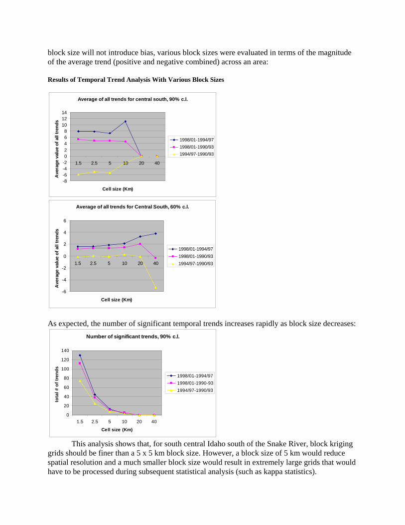
block size will not introduce bias, various block sizes were evaluated in terms of the magnitude of the average trend (positive and negative combined) across an area: Results of Temporal Trend Analysis With Various Block Sizes

Average of all trends for central south, 90% c.l.

-8-6-4-202468

101214

1.5 2.5 5 10 20 40

Cell size (Km)

Ave

rage

val

ue o

f all

tren

ds

1998/01-1994/971998/01-1990/931994/97-1990/93

Average of all trends for Central South, 60% c.l.

-6

-4

-2

0

2

4

6

1.5 2.5 5 10 20 40

Cell size (Km)

Ave

rage

val

ue o

f all

tren

ds

1998/01-1994/971998/01-1990/931994/97-1990/93

As expected, the number of significant temporal trends increases rapidly as block size decreases:

Number of significant trends, 90% c.l.

0

20

40

60

80

100

120

140

1.5 2.5 5 10 20 40

Cell size (Km)

tota

l # o

f tre

nds

1998/01-1994/971998/01-1990-931994/97-1990/93

This analysis shows that, for south central Idaho south of the Snake River, block kriging

grids should be finer than a 5 x 5 km block size. However, a block size of 5 km would reduce spatial resolution and a much smaller block size would result in extremely large grids that would have to be processed during subsequent statistical analysis (such as kappa statistics).

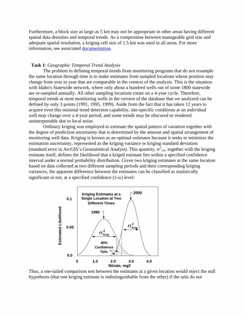
Furthermore, a block size as large as 5 km may not be appropriate in other areas having different spatial data densities and temporal trends. As a compromise between manageable grid size and adequate spatial resolution, a kriging cell size of 1.5 km was used in all areas. For more information, see associated documentation. Task 1: Geographic Temporal Trend Analysis The problem in defining temporal trends from monitoring programs that do not resample the same location through time is to make estimates from sampled locations whose position may change from year to year that are comparable in the context of the analysis. This is the situation with Idaho's Statewide network, where only about a hundred wells out of some 1800 statewide are re-sampled annually. All other sampling locations rotate on a 4-year cycle. Therefore, temporal trends at most monitoring wells in the version of the database that we analyzed can be defined by only 3 points (1991, 1995, 1999). Aside from the fact that it has taken 12 years to acquire even this minimal trend detection capability, site-specific conditions at an individual well may change over a 4-year period, and some trends may be obscured or rendered uninterpretable due to local noise. Ordinary kriging was employed to estimate the spatial pattern of variation together with the degree of prediction uncertainty that is determined by the amount and spatial arrangement of monitoring well data. Kriging is known as an optimal estimator because it seeks to minimize the estimation uncertainty, represented as the kriging variance or kriging standard deviation (standard error in ArcGIS’s Geostatistical Analyst). This quantity, σ2

OK, together with the kriging estimate itself, defines the likelihood that a kriged estimate lies within a specified confidence interval under a normal probability distribution. Given two kriging estimates at the same location based on data collected at two different sampling periods and their corresponding kriging variances, the apparent difference between the estimates can be classified as statistically significant or not, at a specified confidence (1-α) level:

2000

1990

Kriging Estimates at a Single Location at Two

Different Times

Estim

ated

Lik

elih

ood

Nitrate, mg/l

0.1

0.05

0.00 1.0 2.0 3.0 4.0

90%Confidence

Tails

2σ Krig2σ Krig

Thus, a one-tailed comparison test between the estimates at a given location would reject the null hypothesis (that one kriging estimate is indistinguishable from the other) if the tails do not

completely overlap and conclude that a statistically significant change has occurred at that location. In trend analysis, particularly involving water quality variations, it is common practice to accept a higher level of significance (lower confidence level) to test for the existence of a trend in exchange for a lower risk of overlooking trends that are present (increased power of the hypothesis test). Several different levels of significance were compared to evaluate the appropriate confidence level for mapping nitrate trends in the central Idaho area, south of the Snake River (see examples below). Areas Defining Statistically Significant Changes in Nitrate 1990-3 – 1998-01 at 60% Confidence:

Areas Defining Statistically Significant Changes in Nitrate 1990-3 – 1998-01 at 75% Confidence:

Corresponding maps at 90% confidence display even smaller areas of statistically significant change. That is, at higher confidence levels, we accept a lower risk of mistakenly concluding that

change has occurred when it has not. At the same time, the complimentary risk of not identifying change where it has occurred, increases. To be as conservative as possible in trend identification, a lower confidence level should be used. Given the magnitude of kriging variances relative to the magnitude of change that is observed between comparison periods (i.e., from 1990-93 to 1998-2001), 67% appeared to provide a conservative trade-off between these complimentary risks, that would not miss potentially real change while still filtering out a large proportion of the apparent changes portrayed in a simple difference map of kriged concentrations (see figure below for an example):

Nampa

Boise

Nampa

Boise

Apparent change innitrate, mg/l

(simple difference)

Treasure Valley Shallow Aquifer

Statistically significantchange in nitrate, mg/l

(at 67% confidence level)

+16

- 8

mg/l

0

+16

- 8

mg/l

Boise

Boise

Treasure Valley Shallow Aquifer1990-93 to 98-01

A statewide summary map of significant temporal change is available for nitrate (over most of the state) and for arsenic in the Treasure Valley shallow and deep aquifers and the Twin Falls area. Nitrate and arsenic project results for individual areas can be accessed from the statewide summaries in the Project Reporting Interface for Task 1 and Task 2, respectively. Task 2: Probability of Exceeding an Action Level Rather than directly kriging measured values to generate concentration estimates, indicator kriging (IK) can be used to estimate the spatial variability of a non-linear transform of the measured values. Each data value, zi, is first transformed to an indicator value, Ii, by comparing it to a threshold value, zc:

if zi > zc, then Ii = 1 if zi < zc, then Ii = 0

The data are thereby separated into two groups: locations that exceed the threshold and those that do not (where the threshold can be an action level, regulatory limit, etc.). Kriging of these indicator-transformed values produces estimates of the probability that zc will be exceeded at a

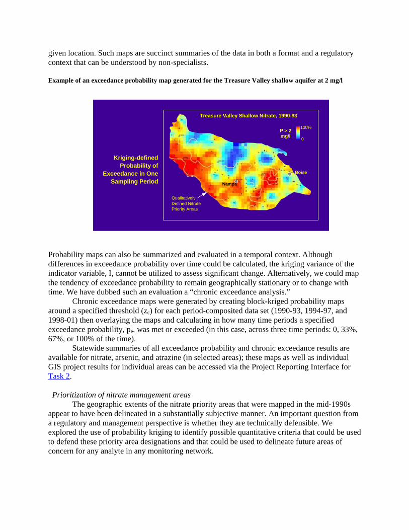
given location. Such maps are succinct summaries of the data in both a format and a regulatory context that can be understood by non-specialists. Example of an exceedance probability map generated for the Treasure Valley shallow aquifer at 2 mg/l

Boise

Nampa

0

100%

Treasure Valley Shallow Nitrate, 1990-93

P > 2 mg/l

QualitativelyDefined NitratePriority Areas

Kriging-definedProbability of

Exceedance in OneSampling Period

Probability maps can also be summarized and evaluated in a temporal context. Although differences in exceedance probability over time could be calculated, the kriging variance of the indicator variable, I, cannot be utilized to assess significant change. Alternatively, we could map the tendency of exceedance probability to remain geographically stationary or to change with time. We have dubbed such an evaluation a “chronic exceedance analysis.” Chronic exceedance maps were generated by creating block-kriged probability maps around a specified threshold (zc) for each period-composited data set (1990-93, 1994-97, and 1998-01) then overlaying the maps and calculating in how many time periods a specified exceedance probability, pe, was met or exceeded (in this case, across three time periods: 0, 33%, 67%, or 100% of the time). Statewide summaries of all exceedance probability and chronic exceedance results are available for nitrate, arsenic, and atrazine (in selected areas); these maps as well as individual GIS project results for individual areas can be accessed via the Project Reporting Interface for Task 2. Prioritization of nitrate management areas

The geographic extents of the nitrate priority areas that were mapped in the mid-1990s appear to have been delineated in a substantially subjective manner. An important question from a regulatory and management perspective is whether they are technically defensible. We explored the use of probability kriging to identify possible quantitative criteria that could be used to defend these priority area designations and that could be used to delineate future areas of concern for any analyte in any monitoring network.

In producing exceedance probability maps from the Statewide database for nitrate at the 2 mg/l threshold, we found that an exceedance probability of 67% was chronically surpassed in areas whose geographic extents were quite similar to previously delineated nitrate priority areas. For example, in the Treasure Valley shallow aquifer:

Calculated from Composited Data1990-93; 1994-97; 1998-01

67% or Greater Probability of

Exceeding 2 mg/l0 3367100% of the time

BoiseNampa

Areas of ChronicExceedance Over

Three Periods

QualitativelyDefined NitratePriority Areas

Nampa

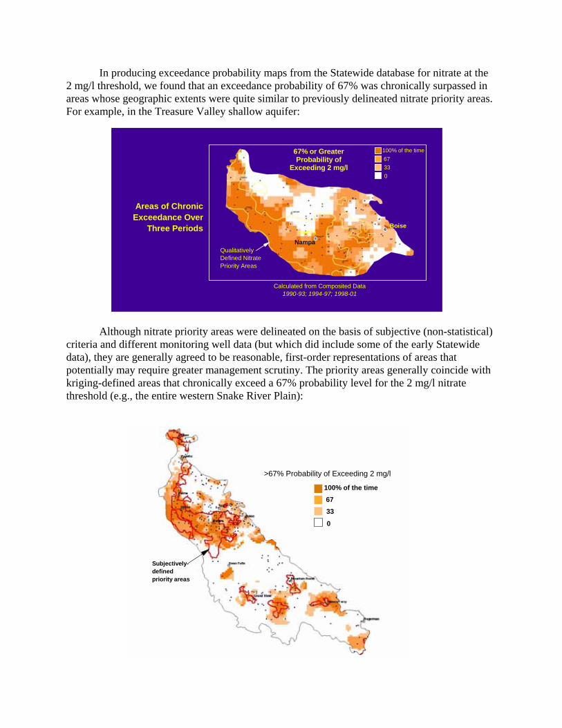
Although nitrate priority areas were delineated on the basis of subjective (non-statistical)

criteria and different monitoring well data (but which did include some of the early Statewide data), they are generally agreed to be reasonable, first-order representations of areas that potentially may require greater management scrutiny. The priority areas generally coincide with kriging-defined areas that chronically exceed a 67% probability level for the 2 mg/l nitrate threshold (e.g., the entire western Snake River Plain):

Subjectively-definedpriority areas

>67% Probability of Exceeding 2 mg/l

0

3367100% of the time

The relative performance of the 33% and 67% chronic exceedance frequencies was evaluated to determine which criterion provides a better match to the subjectively-defined nitrate priority areas. Kappa statistics were calculated from the number of true and false positives and negatives that arise from a cell-by-cell comparison between the subjectively-delineated boundaries and the chronic exceedance areas.

The Use of Chronic Exceedance Frequency to Delineate Nitrate Priority Areas

Exceedanceat least 33%of the time

Exceedanceat least 67%of the time

Subjective priority area 653 1382 Not classified 137 2485

Chronic exceedance Not classified

Subjective priority area 551 776 Not classified 239 3045

Areas of chronic exceedance (2mg/l)

Subjectively- defined priority areas

Agreement rate 66%Kappa coefficient 0.3

Agreement rate 78%Kappa coefficient 0.4

Chronic exceedance Not classified

The results of this evaluation are summarized in the following figure, which compares

classification agreement between the subjectively-defined nitrate priority areas and the chronic exceedance map. The agreement rates and the kappa statistics show that a chronic exceedance frequency of 67% provides better agreement with the currently-defined nitrate priority areas than the 33% exceedance frequency. The agreement rate between the subjectively-delineated areas and mapped areas that exceed a 67% probability of detecting 2 mg/l nitrate more than two-thirds of the time is of the order of 80%, with a kappa coefficient of 0.4 (indicating good agreement between the two classifications).

The following figure shows areas of nitrate concern in the western Snake River Plain as delineated by chronic exceedances of 67% or greater, based on indicator kriging around a 67% probability of exceeding a 2 mg/l threshold:

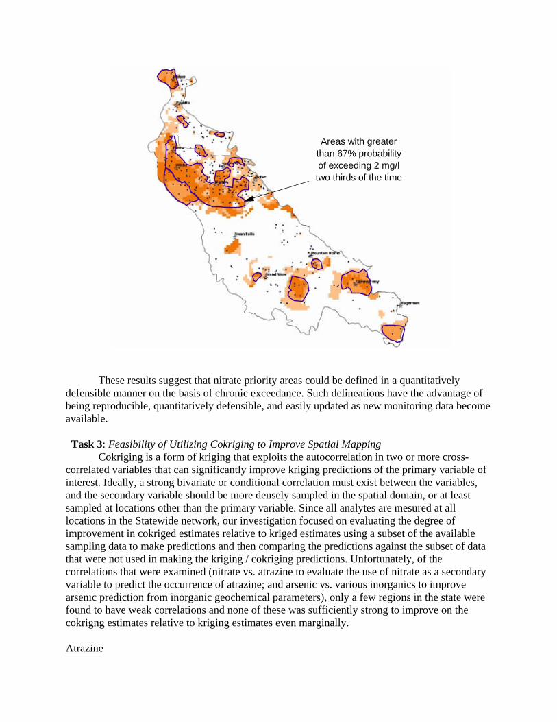
Areas with greaterthan 67% probabilityof exceeding 2 mg/ltwo thirds of the time

These results suggest that nitrate priority areas could be defined in a quantitatively defensible manner on the basis of chronic exceedance. Such delineations have the advantage of being reproducible, quantitatively defensible, and easily updated as new monitoring data become available. Task 3: Feasibility of Utilizing Cokriging to Improve Spatial Mapping Cokriging is a form of kriging that exploits the autocorrelation in two or more cross-correlated variables that can significantly improve kriging predictions of the primary variable of interest. Ideally, a strong bivariate or conditional correlation must exist between the variables, and the secondary variable should be more densely sampled in the spatial domain, or at least sampled at locations other than the primary variable. Since all analytes are mesured at all locations in the Statewide network, our investigation focused on evaluating the degree of improvement in cokriged estimates relative to kriged estimates using a subset of the available sampling data to make predictions and then comparing the predictions against the subset of data that were not used in making the kriging / cokriging predictions. Unfortunately, of the correlations that were examined (nitrate vs. atrazine to evaluate the use of nitrate as a secondary variable to predict the occurrence of atrazine; and arsenic vs. various inorganics to improve arsenic prediction from inorganic geochemical parameters), only a few regions in the state were found to have weak correlations and none of these was sufficiently strong to improve on the cokrigng estimates relative to kriging estimates even marginally. Atrazine

Atrazine, the most commonly detected pesticide in the database. Because it is moderately mobile in most soils, concurrent transport with nitrate through the unsaturated zone might be expected to produce at least a conditional correlation with nitrate (i.e., atrazine is detected more often where nitrate is elevated). No atrazine data were reported for 1990 or 1991; since the database contains only blank entries for these years, blanks were assumed to represent no data. Only six hydrologic subareas contained a sufficient proportion of detects to justify a geostatistical analysis (see worksheet for all calculations and a summary of relationships). Areas 6 and 16 are the only areas with an obvious conditional correlation; contingency table hypothesis tests showed that conditional correlation is marginally better at 2.5 mg/l than at 1mg/l. Area 7 has the greatest atrazine detection rate and the greatest proportion of samples with high atrazine concentrations; conditional correlation is also marginally better at 2.5 mg/l than at 1mg/l. Area 14 is the only case where the correlation is marginally better at 1 mg/l rather than 2.5 mg/l. Analysis was conducted using a chi square contingency table test and a Kappa statistic computed from the error matrix comparing nitrate levels and atrazine detections. No useful bivariate relationships between atrazine and nitrate were found.

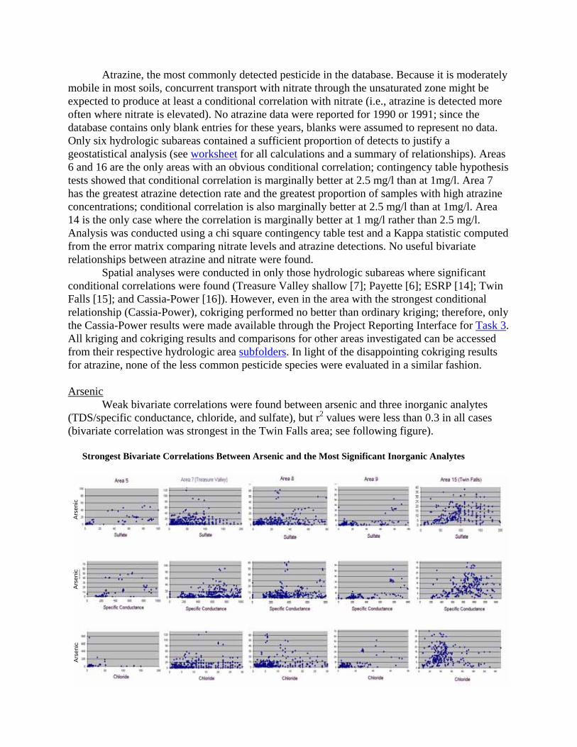
Spatial analyses were conducted in only those hydrologic subareas where significant conditional correlations were found (Treasure Valley shallow [7]; Payette [6]; ESRP [14]; Twin Falls [15]; and Cassia-Power [16]). However, even in the area with the strongest conditional relationship (Cassia-Power), cokriging performed no better than ordinary kriging; therefore, only the Cassia-Power results were made available through the Project Reporting Interface for Task 3. All kriging and cokriging results and comparisons for other areas investigated can be accessed from their respective hydrologic area subfolders. In light of the disappointing cokriging results for atrazine, none of the less common pesticide species were evaluated in a similar fashion. Arsenic Weak bivariate correlations were found between arsenic and three inorganic analytes (TDS/specific conductance, chloride, and sulfate), but r2 values were less than 0.3 in all cases (bivariate correlation was strongest in the Twin Falls area; see following figure). Strongest Bivariate Correlations Between Arsenic and the Most Significant Inorganic Analytes

Ar s

enic

Ars

enic

Ars

enic

Ars

enic

Cokriging prediction performance was evaluated only in the Twin Falls area (using specific conductance as the secondary variable, the best-correlated secondary analyte). No improvement was found between arsenic predictions made by cokriging relative to ordinary kriging; cokriged estimates differed by less than 1 µg/l relative to those obtained by ordinary kriging (see figure, below), and areas of statistically significant difference (even at the 67% confidence level) being so small as to conclude that cokriging with collocated secondary information does not improve estimation performance where such weak bivariate relationships exist. Cokriging (co-OK) of arsenic vs. specific conductance compared with ordinary kriging (OK) of arsenic only:

+1.0

- 0.7

µg/l

Simple Difference, OK vs. C0-OK

Significant Difference (67%)

TwinFallsCounty

TwinFallsCounty

Details of the correlation analyses and cokriging evaluations are accessible via the Project Reporting Interface for Task 3. Spatial-Temporal Kriging The results obtained in Task 1 successfully fulfilled contract requirements by demonstrating how ordinary kriging can be used to map temporal trends in a quantitatively defensible manner. However, the approach does suffer from significant limitations:

a) the use of period-composited sampling data is unsuitable for short time periods where the magnitude of change will be proportionally smaller;

b) it is unsuitable for monitoring networks that are sparsely-sampled in the spatial domain or, like the Statewide network, must be composited because of insufficient spatial coverage in any one sampling event; and

c) it allows only two-point temporal comparisons to be made (one “point” per composited period being compared).

The result is an under-utilization of the network’s information content. That is, by

comparing kriged interpretations of period-composited data, any temporal variations that occur within the span of a 4-year composited time period will be averaged out in the two-point trend comparison. Since the Statewide network provides a decade-long record of water quality at multiple sampling sites (even though all sites are not sampled with the same frequency), it is an ideal data set to investigate the use of a relatively new variant of multi-dimensional geostatistical analysis known as space-time (ST) kriging. The following summary is not intended to provide an exhaustive reporting of either the methodology or the results of ST kriging analysis performed on the Statewide data. The work was conducted as an exploratory extension above and beyond contractual task requirements, but resulted in several developments that may prove to be extremely important for future analysis, modification, and optimization of the Statewide network. The ST kriging work will be reported on through other venues (Non-Point Source Monitoring Workshop, Boise, January, 2004; Geological Society of America regional meeting, Boise, May, 2004; and in peer-reviewed journal articles that are in preparation); this report provides only a summary of the general approach and results.

Statewide nitrate data from the Treasure Valley shallow aquifer were utilized for the evaluation because they are reasonably evenly distributed in space, cover areas of large positive and negative change, and are representative of other areas in the state in terms of sampling density. The most important feature deduced from the analysis is the surprisingly strong temporal autocorrelation. Relative to the spatial semivariogram (whose principal structure has a correlation range of about 4 years; see figure following), the temporal semivariogram appears quite noisy:

σ 2

Temporal (t ) variogramSpatial (x, y) variogram

6.0

4.0

2.0

0.00 5000 10000 15000 20000

Sem

ivar

iogr

am

Distance (meters) or time (years x 1000)

Recalling that the Statewide Network resamples the same wells every four years, however, and that their values tend to remain the same except where affected by temporal trends, we see that

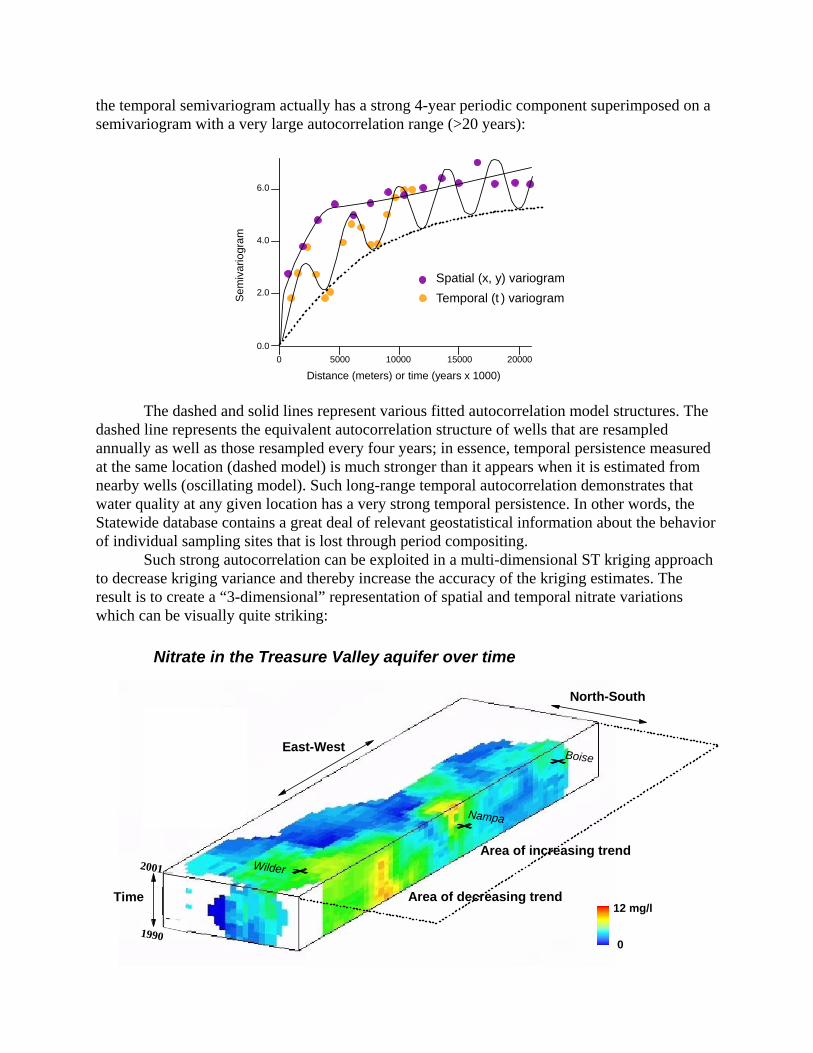
the temporal semivariogram actually has a strong 4-year periodic component superimposed on a semivariogram with a very large autocorrelation range (>20 years):

σ 2

Temporal (t ) variogramSpatial (x, y) variogram

6.0

4.0

2.0

0.00 5000 10000 15000 20000

Sem

ivar

iogr

am

Distance (meters) or time (years x 1000)

The dashed and solid lines represent various fitted autocorrelation model structures. The

dashed line represents the equivalent autocorrelation structure of wells that are resampled annually as well as those resampled every four years; in essence, temporal persistence measured at the same location (dashed model) is much stronger than it appears when it is estimated from nearby wells (oscillating model). Such long-range temporal autocorrelation demonstrates that water quality at any given location has a very strong temporal persistence. In other words, the Statewide database contains a great deal of relevant geostatistical information about the behavior of individual sampling sites that is lost through period compositing. Such strong autocorrelation can be exploited in a multi-dimensional ST kriging approach to decrease kriging variance and thereby increase the accuracy of the kriging estimates. The result is to create a “3-dimensional” representation of spatial and temporal nitrate variations which can be visually quite striking:

Area of decreasing trend

Area of increasing trend

North-South

East-West

Time

Nitrate in the Treasure Valley aquifer over time

Wilder

Nampa

Boise

12 mg/l

01990

2001

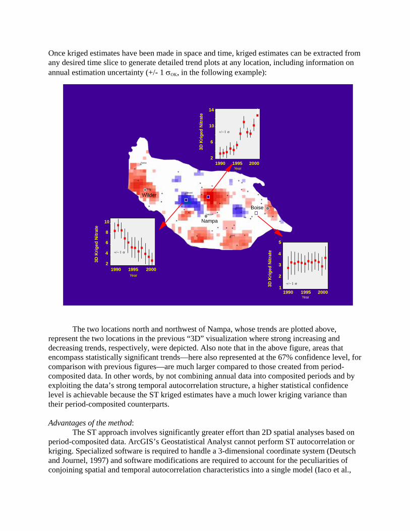
Once kriged estimates have been made in space and time, kriged estimates can be extracted from any desired time slice to generate detailed trend plots at any location, including information on annual estimation uncertainty (+/- 1 σΟΚ, in the following example):

+/− 1 σ

1990 1995 2000Year

2

6

10

14

3D K

riged

Nitr

ate

+/− 1 σ

3D K

riged

Nitr

ate

1990 1995 2000Year

2

4

6

8

10

+/− 1 σ

1990 1995 2000Year

1

2

3

4

5

3D K

riged

Nitr

ate

Boise

Nampa

Wilder

The two locations north and northwest of Nampa, whose trends are plotted above,

represent the two locations in the previous “3D” visualization where strong increasing and decreasing trends, respectively, were depicted. Also note that in the above figure, areas that encompass statistically significant trends—here also represented at the 67% confidence level, for comparison with previous figures—are much larger compared to those created from period-composited data. In other words, by not combining annual data into composited periods and by exploiting the data’s strong temporal autocorrelation structure, a higher statistical confidence level is achievable because the ST kriged estimates have a much lower kriging variance than their period-composited counterparts. Advantages of the method:

The ST approach involves significantly greater effort than 2D spatial analyses based on period-composited data. ArcGIS’s Geostatistical Analyst cannot perform ST autocorrelation or kriging. Specialized software is required to handle a 3-dimensional coordinate system (Deutsch and Journel, 1997) and software modifications are required to account for the peculiarities of conjoining spatial and temporal autocorrelation characteristics into a single model (Iaco et al.,

2003; De Cesare et al., 2002; Kyriakidis and Journel, 1999). Despite these limitations, the ST approach has tremendous advantages over 2D kriging analysis of databases like the Statewide Network.

One of the most important implications is the potential for developing a network optimization scheme based on the ST kriging variance. Future network design modifications are being contemplated by IDWR that may involve new monitoring sites in some areas and a reduction in the number of sites in other, better-characterized areas. As a measure of prediction uncertainty at unsampled locations in a sampling network, kriging variance can be used to optimize the configuration of sampling sites that are required to achieve a given confidence in network coverage (van Groenigen and Stein, 2000). The mean and the dispersion of the kriging variances derived from a network’s sampling configuration can be used to identify where removal and/or addition of selected sampling locations is optimal in terms of network coverage and confidence. Such an approach would provide defensibility for decisions that are ultimately based on sampling cost.

If the strong temporal persistence identified in the Treasure Valley nitrate data is typical of the Statewide Network, then ST kriging could be used to develop a powerful new method of network optimization. Kriging in the ST domain returns much lower local kriging variances than does period-composited kriging in the spatial domain alone. Unlike period compositing which averages temporal variability by projecting data into a composite temporal plane, the ST approach truly utilizes all of the information about spatial and temporal variability in a database. All spatial information has a degree of information redundancy because of its autocorrelated nature. In essence, an ST database (like the Statewide Network’s) has even greater redundancy built into it; strong temporal autocorrelation permits information collected at different sampling times to inform on locations across time just as nearby sampling points inform on each other across space. This characteristic can be exploited to either reduce the number of sampling locations necessary to maintain prediction confidence in unsampled areas or to identify those areas in greatest need of additional sampling points, or both. Summary and Recommendations Results obtained in Tasks 1 and 2 exceeded expectations. The feasibility of kriging was demonstrated as a method of documenting statistically significant temporal trends where direct time-series analysis is not possible, and probabiity mapping was successfully applied to not only represent spatial patterns of variability in a probabilistic form but also as a means to delineate statistically-defensible areas of concern. The outcome of Task 3, unfortunately, did not identify any useful results or approaches that might be useful for database analysis. Spatial Outlier Analysis Prior to kriging, spatial outlier values were identified using spatial statistics. Where high sample values occur in low-valued areas, they can be quickly identified and temporarily filtered out prior to variogram modeling, then reinstated for kriging. In a very few instances, some extremely high nitrate values were withheld for kriging because their influence was deemed unrepresentative of local nitrate levels; such values created strong "bull's eye" patterns over wide areas by their mere presence. Although in some cases such anomalies may be real, they are more

likely due to laboratory, database, or transcriptional errors, and/or problems with sample integrity (e.g., casing leakage, resulting in localized aquifer contamination). Filtering of spatial outliers with ArcGIS's Geostatistical Analyst is a simple and cost-effective means of screening and checking the Statewide database and should be adopted as a routine data evaluation tool. Temporal Change Analysis Based on period-composited data, summary maps of temporal change were created for nitrate over most of the state and for arsenic in the Treasure Valley (shallow and deep) aquifers and in the Twin Falls area. A confidence level of 67% was adopted in all cases to conservatively limit the risk of overlooking areas in which real change did occur. Although information is lost to a degree by compositing data over time periods, the approach has the advantage of being easy to implement in ArcGIS. Results are comparable to those produced using more sophisticated analysis procedures. Probability Mapping This was shown to be a viable method for representing network data in the context of regulatory thresholds (e.g., where is it most likely that regulatory limits or action levels will be exceeded?). By combining probability maps created for multiple years or time periods, a map of chronic exceedance frequency can be generated. Based on this approach, a quantitative and objective method for delineating areas of management concern was developed. We demonstrated that IDEQ’s nitrate priority areas (which were delineated subjectively and without clear documentation or indication of their validity) generally correspond to areas in which it is 67% or more probable that nitrate levels exceed 2 mg/l at least 8 out of 12 years. It is recommended that such an approach (or a modification of it) be adopted--or at least considered--as a tool for delineating management areas that are statistically meaningful and defensible. An additional advantage of the method is that areas of concern so delineated can be periodically updated as new network data become available. Cokriging of Arsenic and Atrazine On the premise that correlations exist between these and other analytes that occur in greater concentration or are detected more frequently, cokriging was investigated as a potential tool for improving mapping performance of these two analytes. Unfortunately, none of the correlations that were identified (either bivariate or conditional) were sufficiently robust to improve prediction performance. For example, the weak conditional correlations between detectable atrazine and nitrate > 2.5 mg/l failed to improve prediction of atrazine detection even marginally. It is postulated that hydrogeologic heterogeneity within the hydrologic subareas into which the Statewide database is segregated is too great, leading to an inability to isolate meaningful correlations within hydrogeologically-similar contexts. For such an approach to work, data from smaller, more densely sampled monitoring programs may have to be considered. Spatial-Temporal Analysis The most significant result of this research has been the surprisingly strong temporal autocorrelation among wells sampled across time. The implication of this is multi-fold: improved prediction performance, reduced prediction uncertainty at unsampled locations, greater statistical confidence levels in classifying temporal trends, and the potential to exploit temporal

autocorrelation in a new and more powerful network design optimization scheme. Although this type of analysis is currently beyond the ability of ArcGIS’s spatial analysis tools and although it requires significantly greater investments of time, effort and expert knowledge to leverage useful information from the database, this approach has the potential to do more for future network data analysis, tools development, and design than any other approach investigated during this project. We strongly recommend that further work be devoted in this area. References Cited De Cesare, L., D.E. Myers, and D. Posa, 2002, FORTRAN programs for space-time modeling; Computers and Geosciences, v. 28, pp. 205-212. De Iaco, S., D.E. Myers, and D. Posa, 2003, The linear coregionalization model and the product-sum space-time variogram; Mathematical Geology, v. 35, pp. 25-38. Isaaks, E.H. and R.M. Srivastava, 1989, An Introduction to Applied Geostatistics; Oxford University Press, New York, 561 pp. Kyriakidis, P.C. and A. G. Journel, 1999, Geostatistical space-time models: a review; Mathematical Geology, v. 31, pp. 651-684. Van Groenigen, J.-W. and A. Stein, 2000, Constrained optimization of spatial sampling in a model-based setting using SANO software; Proc. 4th International Symp on Spatial Accuracy Assessment, Amsterdam, pp. 679-685.