Staining algorithm for seismic modeling and migration

Bo Chen1 and Xiaofeng Jia1

ABSTRACT

In seismic migration, some structures such as those insubsalt shadow zones are not imaged well. The signal inthese areas may be even weaker than the artifacts elsewhere.We evaluated a method to significantly improve the signal-to-noise ratio (S/N) in poorly illuminated areas of the model.We constructed a “phantom” wavefield: an extension of thewavefield to the complex domain. The imaginary wavefieldwas synchronized with the real wavefield, but it containedonly the events relevant to a target region of the model,which was specified using a staining algorithm. The realwavefield interacted with the entire model. However, allstructures except for the target were transparent to the imagi-nary wavefield, which is excited only when the real wave-front arrives at the target structure. The real and theimaginary source wavefields were crosscorrelated with theregular receiver wavefield. The results were revealed intwo images: the conventional reverse time migration imageand an image of the target region only. Synthetic experi-ments showed that the S/N of the target structures was im-proved significantly, with other structures effectively muted.

INTRODUCTION

Seismic migration is one of the most important processing tech-niques that focuses reflections and diffractions and yields seismicimages of subsurface areas. Generally, those images are often usedin further processing and interpretation. However, when dealingwith critical areas such as overhanging structures and subsaltshadow zones, seismic migration may generate poorly focused im-ages. This defect is usually caused by three factors: improper choiceof migration methods, inaccurate estimation of the velocity model,and inadequate data acquisition. Currently, there are three kinds of

migration methods commonly used in practice: ray- or beam-basedmigration, one-way wave-equation-based migration, and full-wave-equation-based migration. Ray-based migration (Albertin et al.,2002; Fowler et al., 2004) can image steep structures effectively;however, it produces relatively low signal-to-noise ratio (S/N) im-ages for subsalt regions. The one-way wave propagator fails to sim-ulate wide-angle and turning waves, which are useful for imagingsteep and overhanging structures (Ristow and Ruhl, 1994; Mulderand Plessix, 2004). Zhang and McMechan (1997) use a horizontalextrapolation scheme to overcome the angle limitation of conven-tional one-way propagators. Tilted coordinates (Sava and Fomel,2005; Shragge and Shan, 2008) can be used to fit the target reflectordip. Jia and Wu (2009) develop a super-wide-angle wavefrontreconstruction method to handle the wide-angle problem and pro-vide good images of steep features and overhanging salt flanks.Based on the two-way wave equation, reverse time migration(RTM) (Baysal et al., 1983; McMechan, 1983; Mulder and Plessix,2004) has excellent performance in steep dip and subsalt imaging inspite of its relatively low efficiency.Apart from the propagator, the poor images of some critical struc-

tures, especially in subsalt regions, are caused by inadequate acquis-ition of seismic signals. Imaging the subsalt area is a challengingproblem because seismic wavefields are strongly distorted whenpropagating through the high-velocity salt bodies. The salt bodycan significantly block the energy, creating uneven illuminationand shadow zones (Jackson et al., 1994; Muerdter and Ratcliff,2001; Leveille et al., 2011; Liu et al., 2011). In such critical subsaltareas, valuable signals are diminished further and are weaker than theartifacts elsewhere. Several approaches have been proposed for im-proving the images of subsalt areas. Illumination compensation forsubsalt imaging (Gherasim et al., 2010; Shen et al., 2011; Yang et al.,2012) can enhance the signals of poorly illuminated subsalt areas.Acquisition aperture correction (Cao and Wu, 2009) can improvethe image amplitude greatly. Malcolm et al. (2008) use multiple scat-tered waves to image subsalt structures that are not easily illuminatedby primaries. Liu et al. (2011) modify conventional RTM and use themultiples as constructive energy for imaging. Velocity model build-

Manuscript received by the Editor 14 July 2013; revised manuscript received 11 March 2014; published online 16 May 2014; corrected version publishedonline 23 May 2014.

1University of Science and Technology of China, School of Earth and Space Sciences, Laboratory of Seismology and Physics of Earth’s Interior, Anhui,China. E-mail: xjia@ustc.edu.cn.

© 2014 Society of Exploration Geophysicists. All rights reserved.

S121

GEOPHYSICS, VOL. 79, NO. 4 (JULY-AUGUST 2014); P. S121–S129, 7 FIGS., 1 TABLE.10.1190/GEO2013-0262.1

Dow

nloa

ded

05/2

4/14

to 1

83.1

60.2

12.9

4. R

edis

trib

utio

n su

bjec

t to

SEG

lice

nse

or c

opyr

ight

; see

Ter

ms

of U

se a

t http

://lib

rary

.seg

.org

/

ing plays an important role to enhance the subsalt visibility and res-olution (Fliedner et al., 2007; Wang et al., 2008; Ji et al., 2011). Atarget-oriented strategy using a data set obtained by generalized Bornmodeling based on a single scattering approximation to the full waveequation can use wavefield-based velocity estimation to focus on im-proving velocities in subsalt regions (Tang and Biondi, 2011). In ad-dition, others focus effort on investigating the impact of acquisitiongeometries on subsalt imaging (Kapoor et al., 2007; VerWest and Lin,2007; Burch et al., 2010; Zhu et al., 2012).In developmental biology, a method called fate mapping (Dale and

Slack, 1987; Gilbert, 2000; Ginhoux et al., 2010) establishes the cor-respondence between individual cells (or groups of cells) at one stageof development and their progeny at later stages of development. Thistechnique is used for understanding the embryonic origin of varioustissues in the adult organism. Embryologists use “vital dyes” (whichwould stain but not harm the cells) to followmovements of individualcells or groups of cells over time in embryos. The tissues to which thecells contribute would thus be labeled and visible in the adult organ-ism. In this paper, we use the concept of fate mapping and implementit in wave propagation. We establish the correspondence between thewavefield and certain desired critical subsurface structures, and wetake advantage of the correspondence to obtain high-quality imagesof the target structures without the influence of other unconcernedstructures. Though not being able to produce true amplitudes cur-rently, this method is a heuristic approach tomanipulate thewavefieldand the imaging process in a useful way.

STAINING ALGORITHM

We propose an algorithm that can trace the wavefront passing atarget structure and identify the origin of a particular reflection. Ifthe wavefront reaches nontarget structures, no response tends to oc-cur as if the medium was transparent; however, once the wavefronttouches the target structure, reflection and transmission occur nor-mally and will be labeled and traced in subsequent propagation. Thewavefront that has touched the target structure can be discriminatedduring propagation, and reflections from the target structure can beidentified and separated in the wavefield or the seismic data. Be-cause this mechanism is like identifying and tracing a single personwho has touched wet paint on a wall from a group of people, wename the method a staining algorithm. In fate mapping, this stain-ing is implemented using dye to stain the cells, which labels andtraces them in subsequent development; however, in seismology,our “dye” is a spatial function that labels the target structure andtraces the wavefront passing the labeled structure.

Wave equation in the complex domain

The equation used in this research is the constant-density 2D fullacoustic wave equation given by

∂2p∂t2

¼ v2Δp; (1)

where Δ ¼ ð∂2∕∂x2 þ ∂2∕∂z2Þ is the Laplace operator, p ¼ pðx;z; tÞ is the pressure wavefield at a spatial location ðx; zÞ and timet, and v ¼ vðx; zÞ is the velocity. To construct a “phantom” wave-field that is synchronized with the real one but only contains thereflections and transmissions relevant to the target structure, we ex-tend all the variables to the complex domain; i.e.,

p ¼ pðx; z; tÞ ¼ p̄þ i ~p; (2)

v ¼ vðx; zÞ ¼ v̄þ i ~v; (3)

where i ¼ ffiffiffiffiffiffi−1

p, the overbar − in all variables denotes the real part,

and the tilde ~denotes the imaginary part. Substituting equations 2and 3 into equation 1, we have the wave equation in the complexdomain expressed as

∂2ðp̄þ i ~pÞ∂t2

¼ ðv̄þ i ~vÞ2ðΔp̄þ iΔ ~pÞ: (4)

Expanding equation 4, we have

∂2ðp̄þ i ~pÞ∂t2

¼ ðv̄2 − ~v2ÞΔp̄ − 2v̄ ~vΔ ~pþ iðv̄2 − ~v2ÞΔ ~p

− 2iv̄ ~vΔp̄: (5)

If ~v → 0, all terms containing ~v can be ignored; thus, equation 5is simplified as

∂2ðp̄þ i ~pÞ∂t2

¼ v̄2Δp̄þ iv̄2Δ ~p ¼ v̄2Δðp̄þ i ~pÞ: (6)

Rewriting equation 6 by separating the real and the imaginaryparts, we have

∂2p̄∂t2

¼ v̄2Δp̄; (7)

∂2 ~p∂t2

¼ v̄2Δ ~p: (8)

We call p̄ the real wavefield and ~p the imaginary wavefield.Comparing equations 7 and 8 with equation 1, we find that p̄and ~p follow the same wave equation, which indicates that theimaginary wavefield is synchronized with the real wavefield inthe propagation.

Excitement and synchronization of the imaginarywavefield

We use the finite-difference (FD) method to solve the wave equa-tion. Denote

plm;n ¼ pðmh; nh; lτÞ; (9)

vm;n ¼ vðmh; nhÞ; (10)

where τ is the time step, h is the grid interval,m and n are the spatialindices, and l is the temporal index. We discuss the second-ordertemporal and spatial accuracy FD scheme for simplicity. The tem-poral derivative is expressed as

∂2p∂t2

����x;z;t

≈1

τ2ðplþ1

m;n − 2plm;n þ pl−1

m;nÞ; (11)

and the spatial derivatives are expressed as

S122 Chen and Jia

Dow

nloa

ded

05/2

4/14

to 1

83.1

60.2

12.9

4. R

edis

trib

utio

n su

bjec

t to

SEG

lice

nse

or c

opyr

ight

; see

Ter

ms

of U

se a

t http

://lib

rary

.seg

.org

/

∂2p∂x2

����x;z;t

≈1

h2ðpl

mþ1;n − 2plm;n þ pl

m−1;nÞ; (12)

∂2p∂z2

����x;z;t

≈1

h2ðpl

m;nþ1 − 2plm;n þ pl

m;n−1Þ: (13)

Substituting equations 11–13 into equation 1, we have the waveequation discretized as

plþ1m;n − 2pl

m;n þ pl−1m;n

¼ v2λ2ðplmþ1;n þ pl

m−1;n þ plm;nþ1 þ pl

m;n−1 − 4plm;nÞ;

(14)

where λ ¼ τ∕h.Hence, the explicit FD iteration scheme is expressed as

plþ1m;n ¼ v2λ2ðpl

mþ1;n þ plm−1;n þ pl

m;nþ1 þ plm;n−1 − 4pl

m;nÞþ 2pl

m;n − pl−1m;n: (15)

Denoting

Pl ¼ λ2ðplmþ1;n þ pl

m−1;n þ plm;nþ1 þ pl

m;n−1 − 4plm;nÞ;

(16)

the iteration scheme can be simplified as

plþ1m;n ¼ v2Pl þ 2pl

m;n − pl−1m;n: (17)

To implement the staining algorithm, we extend all the variablesto the complex domain; i.e.,

plm;n ¼ p̄l

m;n þ i ~plm;n; (18)

Pl ¼ P̄l þ i ~Pl; (19)

vm;n ¼ v̄m;n þ i ~vm;n. (20)

Substituting equations 18–20 into equation 17, we have the iter-ation scheme in the complex domain expressed as

ðp̄lþ1m;n þ i ~plþ1

m;nÞ ¼ ðv̄m;n þ i ~vm;nÞ2ðP̄l þ i ~PlÞþ 2ðp̄l

m;n þ i ~plm;nÞ − ðp̄l−1

m;n þ i ~pl−1m;nÞ: (21)

According to equation 21, the iteration schemes in the real andthe imaginary domains are expressed as follows:

p̄lþ1m;n ¼ v̄2m;nP̄l þ 2p̄l

m;n − p̄l−1m;n − 2v̄m;n ~vm;n

~Pl − ~v2m;nP̄l;

(22)

~plþ1m;n ¼ v̄2m;n

~Pl þ 2 ~plm;n − ~pl−1

m;n þ 2v̄m;n ~vm;nP̄l − ~v2m;n~Pl:

(23)

For the real-domain FD iteration (equation 22), in the computa-tion of the real wavefield, the source is injected by adding the dis-cretized wavelet directly to the wavefield; i.e.,

p̄lþ1m;n ¼ v̄2m;nP̄l þ 2p̄l

m;n − p̄l−1m;n − 2v̄m;n ~vm;n

~Pl

− ~v2m;nP̄l þ slþ1re ; (24)

where slþ1re is the discretized source wavelet. As mentioned above,

theoretically, all terms containing ~vm;n can be ignored if ~vm;n → 0.To quantitatively analyze the influence of ~vm;n, we define

γðkÞ ¼ max jpðx; zÞ − p̄ðkÞðx; zÞjmax jpðx; zÞj ; (25)

where pðx; zÞ is the wavefield calculated in the conventional wayusing the wave equation in the real domain and p̄ðkÞðx; zÞ is calcu-lated by equation 24 with ~vm;n k orders of magnitude smaller thanv̄m;n. The term γðkÞ is a key factor to determine the order of mag-nitude of ~vm;n in the computation. The staining mechanism is imple-mented by assigning an infinitesimal value to the imaginary part ofthe velocity; i.e.,

v̄m;n ¼ vm;n; ~vm;n

�≠ 0; target structure

¼ 0; otherwise: (26)

Practically, when ~vm;n is of the 10−6 order of magnitude, γðkÞ iszero with the computer program using single-precision real-typevariables. In this case, we can ignore the terms of ~vm;n in equation 24and obtain the real-domain iteration scheme:

p̄lþ1m;n ¼ v̄2m;nP̄l þ 2p̄l

m;n − p̄l−1m;n þ slþ1

re : (27)

For the imaginary-domain FD iteration equation 23, we can firstignore the second-order term ~v2m;nP̄l. Equation 23 can be written as

~plþ1m;n ¼ v̄2m;n

~Pl þ 2 ~plm;n − ~pl−1

m;n þ 2v̄m;n ~vm;nP̄l: (28)

We now discuss the property of the term 2v̄m;n ~vm;nP̄l and how~pm;n is excited. For any point except for the source location, p̄0

m;n ¼p̄−1m;n ¼ 0 and ~p0

m;n ¼ ~p−1m;n ¼ 0. Suppose only one single point

ðm0; n0Þ is stained, i.e., ~vm0;n0 ≠ 0, and the first arrival in the realdomain comes at the time step l0; i.e., p̄l

m0 ;n0 ¼ 0 when l < l0. Ac-cording to equation 28, if and only if ~vm;n ≠ 0 and P̄l ≠ 0, i.e.,2v̄m;n ~vm;nP̄l ≠ 0, the imaginary wavefield can be excited. Thatis, the imaginary wavefield is generated once the real wavefieldhits the stained target. When the wavefront in the real domainhas passed the stained point ðm0; n0Þ, P̄l becomes zero, leadingto 2v̄m;n ~vm;nP̄l ¼ 0. Consequently, the term 2v̄m;n ~vm;nP̄l can be re-garded as a source term injected automatically by the staining algo-rithm. We have equation 28 rewritten as

~plþ1m;n ¼ v̄2m;n

~Pl þ 2 ~plm;n − ~pl−1

m;n þ slþ1im ; (29)

where slþ1m;n ¼ 2v̄m;n ~vm;nP̄l.

Comparing equation 27 with equation 29, we find that p̄m;n and~pm;n have the same iteration scheme, which indicates that the imagi-nary wavefield is synchronized with the real wavefield and excitedat the stained structure. In the real domain, the wavefront propagatesnormally without interference. Meanwhile, in the imaginary do-main, only when the wavefront in the real domain arrives at thestained target structure (where ~vm;n ≠ 0) are the stained points trig-gered as point sources. According to Huygens’ principle (Sheriffand Geldart, 1995), every point on a wavefront can be regarded

Staining algorithm S123

Dow

nloa

ded

05/2

4/14

to 1

83.1

60.2

12.9

4. R

edis

trib

utio

n su

bjec

t to

SEG

lice

nse

or c

opyr

ight

; see

Ter

ms

of U

se a

t http

://lib

rary

.seg

.org

/

as a new source of waves. Thus, the imaginary wavefield is excitedby these point sources and synchronized with the real wavefield inthe subsequent propagation as demonstrated in equations 27 and 29.The selectively excited imaginary wavefield can provide phase in-formation mapping to the real wavefield; thus, all responses relatedto the target structure are “stained” and can be traced and identified.We call the surface data obtained in the real domainDreðx; z ¼ 0; tÞreal data, and the data obtained in the imaginary domainDimðx; z ¼ 0; tÞ imaginary data. According to the excitement ofthe imaginary wavefield, imaginary data are synchronized withand are part of the real data.

Imaging condition

The staining algorithm can be applied to seismic migration toobtain an image of the target structure. The migration method usedin this study is RTM, which consists of three main steps (Symes,2007): (1) extrapolate the forward-propagating shot wavefieldSðx; z; tÞ, (2) extrapolate the backward-propagating receiver wave-field Gðx; z; tÞ, and (3) apply the imaging condition to obtain theimage. We can apply the staining algorithm by modifying steps1 and 3. The receiver wavefield is computed conventionally inthe real domain with recorded data as virtual sources. However,the shot wavefield is computed in the complex domain with thestained complex velocity model, and the real shot wavefieldSreðx; z; tÞ and the imaginary shot wavefield Simðx; z; tÞ are ob-tained together. Subsequently, the two shot wavefields are crosscor-related with the conventional receiver wavefield, respectively.Imaging conditions can be expressed as

Ireðx; zÞ ¼Z

T

0

Sreðx; z; tÞGðx; z; T − tÞdt; (30)

Iimðx; zÞ ¼Z

T

0

Simðx; z; tÞGðx; z; T − tÞdt; (31)

where Gðx; z; tÞ is the receiver wavefield. The term Ireðx; zÞ is thereal image that is exactly the same as the result of conventionalRTM, and Iimðx; zÞ is the imaginary image that can be consideredas the image of the target region.

NUMERICAL EXAMPLES

We have conducted numerical experiments on a series of velocitymodels to show the application of the staining algorithm to seismicmodeling and migration. The propagator used in the experiment isan eighth-order spatial and second-order temporal accuracy explicitFD scheme.Figure 1 shows the excitement and synchronization of the imagi-

nary wavefield. Figure 1a shows a simple model in the complexdomain with the velocities of each layer 2.5, 3.5, and 4.5 km∕s,respectively, in the real part, and the reflector at depth 4.4 kmstained by assigning 1.0 × 10−6 to the imaginary part. The shotis located at 4 km on the surface, and geophones are distributedfrom 0 to 4 km with an interval of 8 m. When the wavefront inthe real domain arrives at the nonstained reflector at 2.4 km, reflec-tion and transmission occur in the real wavefield normally; how-ever, in the imaginary wavefield, no responses occur because nostained structure has been touched yet. When the wavefront inthe real domain arrives at the stained reflector at 4.4 km, the points

on the interface are successively activated and excite the imaginarywavefield as point sources. Figure 1b and 1d shows snapshots of thereal wavefield at 1.8 and 2.2 s, respectively; Figure 1c and 1e showsthe corresponding snapshots of the imaginary wavefield. Compar-ing the snapshots of the real and the imaginary wavefield, we findthat the imaginary wavefield is synchronized with the real wavefieldin propagation after being excited. Because the imaginary wavefieldis not excited before the wavefront in the real domain arrives at thestained interface, it only contains the reflection and transmissionrelevant to the stained reflector excluding the ones relevant to othernonstained structures. Figure 2 shows the seismograms of the realand the imaginary wavefields recorded at the point (4 km, 2.4 km).The response at 1.032 s in the real domain is the direct arrival to thereflector at 2.4 km, and the response at 2.175 s is the reflection fromthe stained reflector at 4.4 km. The imaginary wavefield is not ex-cited until the wavefront arrives at the stained reflector at 1.603 s.Consequently, the directly arrival does not appear in the imaginarydomain and only the reflection from the stained reflector is re-corded. The reflection in the imaginary domain is synchronizedwith that in the real domain.Figure 3 shows the difference of the wavefield calculated in the

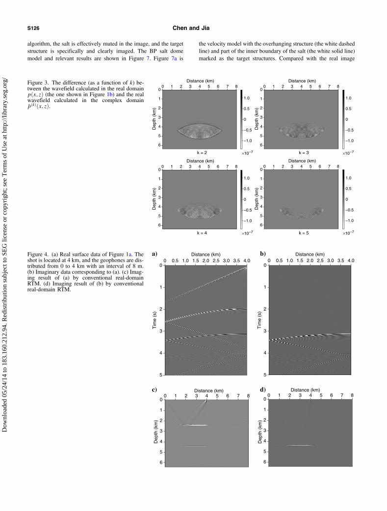
conventional real domain and the corresponding real wavefield cal-culated in the complex domain, i.e., pðx; zÞ − p̄ðkÞðx; zÞ. The imagi-nary velocity ~vm;n used for the calculation ranges from 2 to 5 ordersof magnitude smaller than the real velocity v̄m;n. The differenceillustrated in the figure is the ignored term in equation 22. Whenthe order of magnitude reduces to 10−6 (i.e., k ¼ 6), the differencebecomes zero in the computation using single-precision real-typevariables, which indicates that the real wavefield calculated bystaining algorithm is not affected by the imaginary one and is iden-tical to the one calculated in the conventional way. Table 1 showsthe magnitude of the maximal difference and γðkÞ with the variationof k corresponding to Figure 1b.Figure 4a and 4b shows the real surface data and the imaginary

data of Figure 1a, respectively. In the imaginary data, the directwave and responses from the reflector at 2.4 km are absent as ifthe medium above the stained interface was transparent. Figure 4cand 4d is obtained using the real and imaginary data above, respec-tively, for conventional real-domain RTM. Compared with Fig-ure 4c, the reflector at 2.4 km is not imaged in Figure 4d, whichproves that the imaginary data only contain the reflections relevantto the stained interface.The results of a complex velocity model are shown in Figure 5.

Figure 5a is the Sigsbee2A model, in which the sediment betweenthe two white arrows is the stained target structure. Figure 5b and 5cshows the real and imaginary data, respectively. The shot is locatedat 13.26 km, and the geophones are distributed from 0 to 24.39 kmwith an interval of 11.43 m. Figure 5d and 5e is obtained using thedata shown in Figure 5b and 5c, respectively, for conventional real-domain RTM. From the tests above, we can see the imaginary wave-field and the imaginary data obtained by staining algorithm onlycontain the responses relevant to the stained target structure.Figures 6 and 7 show the application of the staining algorithm to

migration. In these tests, all the data used for the computation areconventional recorded data, not the imaginary data we generated bythe staining algorithm and those used in the previous tests. The realimage and the imaginary image are obtained from the same data set,and by imaging condition equations 30 and 31, respectively. Somecritical structures are selected to verify the validity of the staining

S124 Chen and Jia

Dow

nloa

ded

05/2

4/14

to 1

83.1

60.2

12.9

4. R

edis

trib

utio

n su

bjec

t to

SEG

lice

nse

or c

opyr

ight

; see

Ter

ms

of U

se a

t http

://lib

rary

.seg

.org

/

algorithm in migration. The results of the numerical test on theSEG/EAGE model are shown in Figure 6. The target subsalt struc-ture is marked in the model shown in Figure 6a. The real image (thesame as the one by conventional RTM) and the imaginary image

(image of the target structure) are obtained simultaneously, and theyare shown in Figure 6b and 6c, respectively. Due to weak illumi-nation and the masking of the salt above, the structure under the saltis not well imaged by conventional RTM. By using the staining

0 0.5 1 1.5 2 2.5 3−1

−0.5

0

0.5

1

Time (s)

Nor

mal

ized

am

plitu

de

0 0.5 1 1.5 2 2.5 3−1

−0.5

0

0.5

1

Time (s)

Nor

mal

ized

am

plitu

de

Figure 2. Seismogram in the real (the top) and theimaginary (the bottom) domains recorded at(4 km, 2.4 km). The record length is 3 s, andthe amplitude of each is normalized to 1. Thesource is a Ricker wavelet with dominant fre-quency of 40 Hz and time shift of 0.072 s.

0

1

2

3

4

5

6

Dep

th (

km)

Distance (km)

2.5 3.0 3.5 4.0 4.5Velocity (km/s)

0 1

a)

b) c)

d) e)

2 3 4 5 6 7 0 1 2 3 4 5 6 7 8

Distance (km)

0 0.2 0.4 0.6 0.8 1.0×10–6

Velocity (km/s)

0

1

2

3

4

5

6

Dep

th (

km)

Distance (km)

–0.002

–0.001

0

0.001

0.002

0.003

0.0040

1

2

3

4

5

6

Dep

th (

km)

Distance (km)

–4

–2

0

2

4

×10–10

0

1

2

3

4

5

6

Dep

th (

km)

Distance (km)

–0.002

–0.001

0

0.001

0.002

0.003

0.0040

1

2

3

4

5

6

Dep

th (

km)

0 1 2 3 4 5 6 7 8 0 1 2 3 4 5 6 7 8

0 1 2 3 4 5 6 7 8 0 1 2 3 4 5 6 7 8Distance (km)

–4

–2

0

2

4

×10–10

Figure 1. (a) Stained velocity model in the com-plex domain. The left is the real part with veloc-ities of each layer 2.5, 3.25, and 4.5 km∕s,respectively. The right is the imaginary part withthe points on the reflector at 4.4 km 1.0 × 10−6 andelsewhere zero. (b) Snapshot of the real wavefieldat 1.8 s. (c) Snapshot of the imaginary wavefieldcorresponding to (b). (d) Snapshot of the realwavefield at 2.2 s. (e) Snapshot of the imaginarywavefield corresponding to (d).

Staining algorithm S125

Dow

nloa

ded

05/2

4/14

to 1

83.1

60.2

12.9

4. R

edis

trib

utio

n su

bjec

t to

SEG

lice

nse

or c

opyr

ight

; see

Ter

ms

of U

se a

t http

://lib

rary

.seg

.org

/

algorithm, the salt is effectively muted in the image, and the targetstructure is specifically and clearly imaged. The BP salt domemodel and relevant results are shown in Figure 7. Figure 7a is

the velocity model with the overhanging structure (the white dashedline) and part of the inner boundary of the salt (the white solid line)marked as the target structures. Compared with the real image

0

1

2

3

4

5

6

Dep

th (

km)

Distance (km)

–1.0

–0.5

0

0.5

1.0

×10–7

0

1

2

3

4

5

6

Dep

th (

km)

Distance (km)

–1.0

–0.5

0

0.5

1.0

×10–7

0

1

2

3

4

5

6

Dep

th (

km)

Distance (km)

–1.0

–0.5

0

0.5

1.0

×10–7

0

1

2

3

4

5

6

Dep

th (

km)

0 1 2 3 4 5 6 7 8

0 1 2 3 4 5 6 7 8 0 1 2 3 4 5 6 7 8

0 1 2 3 4 5 6 7 8

Distance (km)

–1.0

–0.5

0

0.5

1.0

×10–7

k = 2 k = 3

k = 4 k = 5

Figure 3. The difference (as a function of k) be-tween the wavefield calculated in the real domainpðx; zÞ (the one shown in Figure 1b) and the realwavefield calculated in the complex domainp̄ðkÞðx; zÞ.

0

1

2

3

4

5

Tim

e (s

)

0 0.5 1.0 1.5 2.0 2.5 3.0 3.5 4.0Distance (km)

0

1

2

3

4

5

Tim

e (s

)0 0.5 1.0 1.5 2.0 2.5 3.0 3.5 4.0

Distance (km)

0

1

2

3

4

5

6

Dep

th (

km)

Distance (km)

0

1

2

3

4

5

6

Dep

th (

km)

0 1 2 3 4 5 6 7 8 0 1 2 3 4 5 6 7 8Distance (km)

a) b)

c) d)

Figure 4. (a) Real surface data of Figure 1a. Theshot is located at 4 km, and the geophones are dis-tributed from 0 to 4 km with an interval of 8 m.(b) Imaginary data corresponding to (a). (c) Imag-ing result of (a) by conventional real-domainRTM. (d) Imaging result of (b) by conventionalreal-domain RTM.

S126 Chen and Jia

Dow

nloa

ded

05/2

4/14

to 1

83.1

60.2

12.9

4. R

edis

trib

utio

n su

bjec

t to

SEG

lice

nse

or c

opyr

ight

; see

Ter

ms

of U

se a

t http

://lib

rary

.seg

.org

/

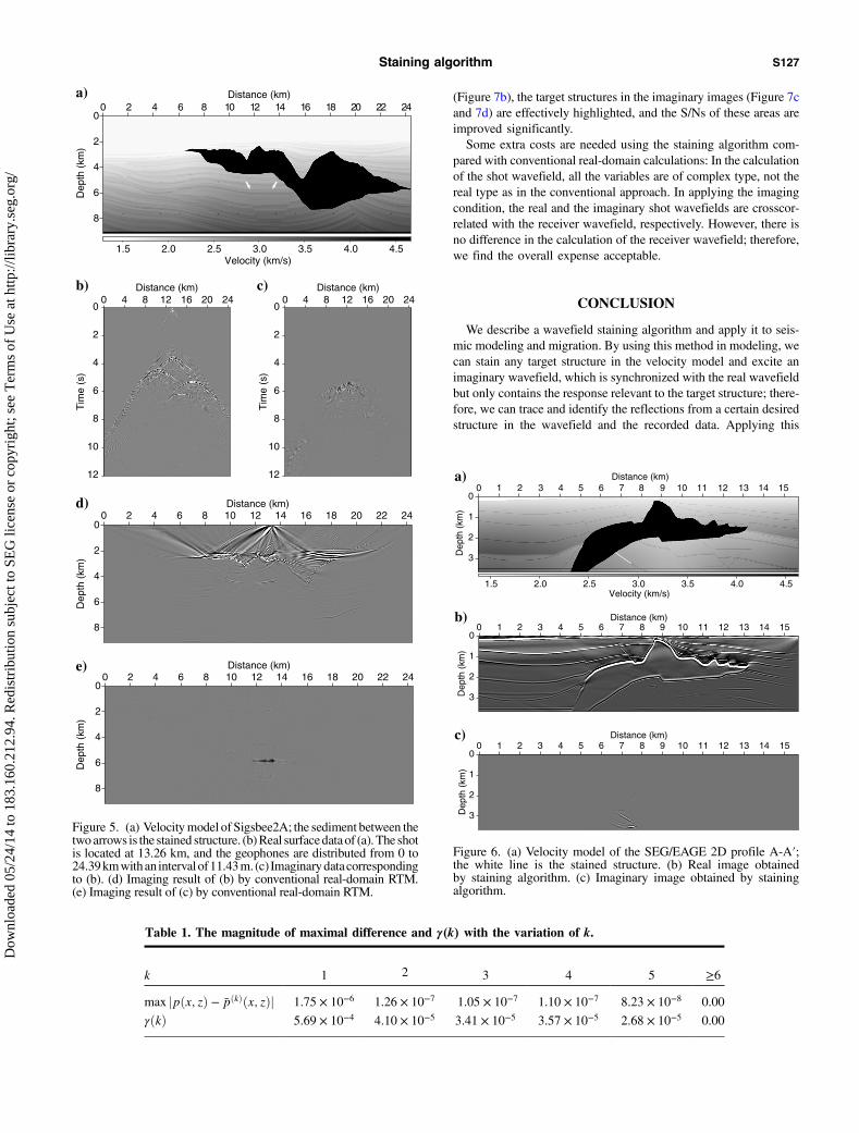
(Figure 7b), the target structures in the imaginary images (Figure 7cand 7d) are effectively highlighted, and the S/Ns of these areas areimproved significantly.Some extra costs are needed using the staining algorithm com-

pared with conventional real-domain calculations: In the calculationof the shot wavefield, all the variables are of complex type, not thereal type as in the conventional approach. In applying the imagingcondition, the real and the imaginary shot wavefields are crosscor-related with the receiver wavefield, respectively. However, there isno difference in the calculation of the receiver wavefield; therefore,we find the overall expense acceptable.

CONCLUSION

We describe a wavefield staining algorithm and apply it to seis-mic modeling and migration. By using this method in modeling, wecan stain any target structure in the velocity model and excite animaginary wavefield, which is synchronized with the real wavefieldbut only contains the response relevant to the target structure; there-fore, we can trace and identify the reflections from a certain desiredstructure in the wavefield and the recorded data. Applying this

0

1

2

3Dep

th (

km)

0 10 11 12 13 14 15Distance (km)

1.5 2.0 2.5 3.0 3.5 4.0 4.5Velocity (km/s)

0

1

2

3Dep

th (

km)

0 10 11 12 13 14 15Distance (km)

0

1

2

3Dep

th (

km)

0

1 2 3 4 5 6 7 8 9

1 2 3 4 5 6 7 8 9

1 2 3 4 5 6 7 8 9 10 11 12 13 14 15Distance (km)

a)

b)

c)

Figure 6. (a) Velocity model of the SEG/EAGE 2D profile A-A′;the white line is the stained structure. (b) Real image obtainedby staining algorithm. (c) Imaginary image obtained by stainingalgorithm.

Table 1. The magnitude of maximal difference and γ�k� with the variation of k.

k 1 2 3 4 5 ≥6

max jpðx; zÞ − p̄ðkÞðx; zÞj 1.75 × 10−6 1.26 × 10−7 1.05 × 10−7 1.10 × 10−7 8.23 × 10−8 0.00

γðkÞ 5.69 × 10−4 4.10 × 10−5 3.41 × 10−5 3.57 × 10−5 2.68 × 10−5 0.00

0

a)

b)

d)

e)

c)

2

4

6

8

Dep

th (

km)

0 2 4 6 8 10 12 14 16 18 20 22 24Distance (km)

1.5 2.0 2.5 3.0 3.5 4.0 4.5Velocity (km/s)

0

2

4

6

8

10

12

Tim

e (s

)

Distance (km)

0

2

4

6

8

10

12

Tim

e (s

)

0 4 8 12 16 20 240 4 8 12 16 20 24Distance (km)

0

2

4

6

8

Dep

th (

km)

0 2 4 6 8 10 12 14 16 18 20 22 24Distance (km)

0

2

4

6

8

Dep

th (

km)

0 2 4 6 8 10 12 14 16 18 20 22 24Distance (km)

Figure 5. (a) Velocitymodel of Sigsbee2A; the sediment between thetwoarrows is the stained structure. (b)Real surfacedataof (a). The shotis located at 13.26 km, and the geophones are distributed from 0 to24.39kmwithan interval of11.43m. (c) Imaginarydatacorrespondingto (b). (d) Imaging result of (b) by conventional real-domain RTM.(e) Imaging result of (c) by conventional real-domain RTM.

Staining algorithm S127

Dow

nloa

ded

05/2

4/14

to 1

83.1

60.2

12.9

4. R

edis

trib

utio

n su

bjec

t to

SEG

lice

nse

or c

opyr

ight

; see

Ter

ms

of U

se a

t http

://lib

rary

.seg

.org

/

method to migration, we can effectively mute reflections of nontar-get structures in the imaginary shot wavefield. Beside the conven-tional RTM image, we can simultaneously obtain an image of thetarget region with the S/N significantly improved. Numerical exam-ples on various models give satisfactory modeling and imaging re-sults. Implementation of this method is easy and independent of aspecific migration operator. It can be easily used by any popularmigration approach to enhance the image quality of critical struc-tures. This method is also potential in quantitative illuminationanalysis and velocity model building.

ACKNOWLEDGMENTS

The authors thank the Subsalt Multiple Attenuation and Reduc-tion Technology Joint Venture for providing the Sigsbee2A syn-thetic data set and BP for providing the 2004 BP 2D syntheticdata set. We particularly acknowledge J. Etgen for polishing themanuscript, and we thank him and two anonymous reviewers fortheir valuable comments and constructive suggestions. We aregrateful to T. Hu and H.-W. Chen for their fruitful discussions. Thisstudy received support from the National Natural Science Founda-tion of China (no. 41004045) and the Knowledge Innovation Pro-gram of the Chinese Academy of Sciences (no. KZCX2-EW-QN503). Our work was also supported by the Chinese Academyof Sciences and State Administration of Foreign Experts AffairsInternational Partnership Program for Creative Research Teams.

REFERENCES

Albertin, U., D. Watts, W. Chang, S. J. Kapoor, C. Stork, P. Kitchenside, andD. Yingst, 2002, Near-salt-flank imaging with Kirchhoff and wavefieldextrapolation migration: 72nd Annual International Meeting, SEG, Ex-panded Abstracts, 1328–1331.

Baysal, E., D. D. Kosloff, and J. W. C. Sherwood, 1983, Reverse time mi-gration: Geophysics, 48, 1514–1524, doi: 10.1190/1.1441434.

Burch, T., B. Hornby, H. Sugianto, and B. Nolte, 2010, Subsalt 3D VSPimaging at Deimos Field in the deepwater Gulf of Mexico: The LeadingEdge, 29, 680–685, doi: 10.1190/1.3447781.

Cao, J., and R. S. Wu, 2009, Fast acquisition aperture correction in prestackdepth migration using beamlet decomposition: Geophysics, 74, no. 4,S67–S74, doi: 10.1190/1.3116284.

Dale, L., and J. M. W. Slack, 1987, Fate map for the 32-cell stage of Xen-opus laevis: Development, 99, 527–551.

Fliedner, M., M. Brown, D. Bevc, and B. Biondi, 2007, Wavepath tomog-raphy for subsalt velocity-model building: 77th Annual InternationalMeeting, SEG, Expanded Abstracts, 1938–1942.

Fowler, P. J., E. Mobley, and B. Hootman, 2004, The importance ofanisotropy and turning rays in prestack time migration: 74th AnnualInternational Meeting, SEG, Expanded Abstracts, 1013–1016.

Gherasim, M., U. Albertin, B. Nolte, and O. Askim, 2010, Wave-equationangle-based illumination weighting for optimized subsalt imaging: 80thAnnual International Meeting, SEG, Expanded Abstracts, 3293–3297.

Gilbert, S. F., 2000, Developmental biology, 6th ed.: Sinauer Associates.Ginhoux, F.,M.Greter,M.Leboeuf, S.Nandi, P. See, S.Gokhan,M. F.Mehler,

S. J. Conway, L. G. Ng, E. R. Stanley, I. M. Samokhvalov, and M. Merad,2010, Fate mapping analysis reveals that adult microglia derive from primi-tive macrophages: Science, 330, 841–845, doi: 10.1126/science.1194637.

Jackson, M. P. A., B. C. Vendeville, and D. D. Schultz-Ela, 1994, Salt-re-lated structures in the Gulf of Mexico: A field guide for geophysicists: TheLeading Edge, 13, 837–842, doi: 10.1190/1.1437040.

Ji, S., T. Huang, K. Fu, and Z. Li, 2011, Dirty salt velocity inversion: Theroad to a clearer subsalt image: Geophysics, 76, no. 5, WB169–WB174,doi: 10.1190/geo2010-0392.1.

0

2

4

6

8

10

Dep

th (

km)

20 22 24 26 28 30 32 34 36 38 40 42 44Distance (km)

1.5 2.0 2.5 3.0 3.5 4.0 4.5Velocity (km/s)

0

2

4

6

8

10

Dep

th (

km)

20 22 24 26 28 30 32 34 36 38 40 42 44Distance (km)

0

2

4

6

8

10

Dep

th (

km)

20 22 24 26 28 30 32 34 36 38 40 42 44Distance (km)

0

2

4

6

8

10

Dep

th (

km)

20 22 24 26 28 30 32 34 36 38 40 42 44Distance (km)

a) b)

c) d)

Figure 7. (a) Velocity model of BP 2D benchmark data set; the white dashed line is the stained structure 1, and the white solid line is thestrained structure 2. (b) Real image obtained by staining algorithm. (c) Imaginary image obtained by staining algorithm (target 1). (d) Imaginaryimage obtained by staining algorithm (target 2).

S128 Chen and Jia

Dow

nloa

ded

05/2

4/14

to 1

83.1

60.2

12.9

4. R

edis

trib

utio

n su

bjec

t to

SEG

lice

nse

or c

opyr

ight

; see

Ter

ms

of U

se a

t http

://lib

rary

.seg

.org

/

Jia, X., and R. S. Wu, 2009, Superwide-angle one-way wave propagator andits application in imaging steep salt flanks: Geophysics, 74, no. 4, S75–S83, doi: 10.1190/1.3124686.

Kapoor, J., N. Moldevaneau, M. Egan, M. O’Briain, D. Desta, I. Atakish-iyev, M. Tomida, and L. Stewart, 2007, Subsalt imaging: The RAZ-WAZ experience: The Leading Edge, 26, 1414–1422, doi: 10.1190/1.2805764.

Leveille, J., I. Jones, Z. Zhou, B. Wang, and F. Liu, 2011, Subsalt imagingfor exploration, production, and development: A review: Geophysics, 76,no. 5, WB3–WB20, doi: 10.1190/geo2011-0156.1.

Liu, Y., X. Chang, D. Jin, R. He, H. Sun, and Y. Zheng, 2011, Reverse timemigration of multiples for subsalt imaging: Geophysics, 76, no. 5,WB209–WB216, doi: 10.1190/geo2010-0312.1.

Malcolm, A. E., B. Ursin, and M. V. de Hoop, 2008, Subsalt imaging withinternal multiples: 78th Annual International Meeting, SEG, ExpandedAbstracts, 2461–2465.

McMechan, G. A., 1983, Migration by extrapolation of time-dependentboundary values: Geophysical Prospecting, 31, 413–420, doi: 10.1111/j.1365-2478.1983.tb01060.x.

Muerdter, D., and D. Ratcliff, 2001, Understanding subsalt illuminationthrough ray-trace modeling, Part 1: Simple 2-D salt models: The LeadingEdge, 20, 578–594, doi: 10.1190/1.1438998.

Mulder, W. A., and R.-E. Plessix, 2004, A comparison between one-way andtwo-way wave-equation migration: Geophysics, 69, 1491–1504, doi: 10.1190/1.1836822.

Ristow, D., and T. Ruhl, 1994, Fourier finite-difference migration: Geophys-ics, 59, 1882–1893, doi: 10.1190/1.1443575.

Sava, P., and S. Fomel, 2005, Riemannian wavefield extrapolation: Geo-physics, 70, no. 3, T45–T56, doi: 10.1190/1.1925748.

Shen, H., S. Mothi, and U. Albertin, 2011, Improving subsalt imaging withillumination-based weighting of RTM 3D angle gathers: 81st AnnualInternational Meeting, SEG, Expanded Abstracts, 3206–3211.

Sheriff, R. E., and L. P. Geldart, 1995, Exploration seismology, 2nd ed.:Cambridge University Press.

Shragge, J., and G. Shan, 2008, Prestack wave-equation depth migration inelliptical coordinates: Geophysics, 73, no. 5, S169–S175, doi: 10.1190/1.2956349.

Symes, W. W., 2007, Reverse time migration with optimal checkpointing:Geophysics, 72, no. 5, SM213–SM221, doi: 10.1190/1.2742686.

Tang, Y., and B. Biondi, 2011, Target-oriented wavefield tomography usingsynthesized Born data: Geophysics, 76, no. 5, WB191–WB207, doi: 10.1190/geo2010-0383.1.

VerWest, B., and D. Lin, 2007, Modeling the impact of wide-azimuth ac-quisition on subsalt imaging: Geophysics, 72, no. 5, SM241–SM250, doi:10.1190/1.2736516.

Wang, B., Y. Kim, C. Mason, and X. Zeng, 2008, Advances in velocitymodel-building technology for subsalt imaging: Geophysics, 73, no. 5,VE173–VE181, doi: 10.1190/1.2966096.

Yang, T. N., J. Shragge, and P. Sava, 2012, Illumination compensation forsubsalt image-domain wavefield tomography: 82nd Annual InternationalMeeting, SEG, Expanded Abstracts, doi: 10.1190/segam2012-0563.1.

Zhang, J., and G. A. McMechan, 1997, Turning wave migration by horizon-tal extrapolation: Geophysics, 62, 291–297, doi: 10.1190/1.1444130.

Zhu, X., J. Cao, D. Ashabranner, S. Sood, J. Brewer, and C. Mosher, 2012,Advanced modeling and imaging for seismic acquisition — A GOMsubsalt example: 82nd Annual International Meeting, SEG, ExpandedAbstracts, doi: 10.1190/segam2012-0858.1.

Staining algorithm S129

Dow

nloa

ded

05/2

4/14

to 1

83.1

60.2

12.9

4. R

edis

trib

utio

n su

bjec

t to

SEG

lice

nse

or c

opyr

ight

; see

Ter

ms

of U

se a

t http

://lib

rary

.seg

.org

/