3d wave field extrapolation in seismic depth migration
TRANSCRIPT
3D WAVE FIELD EXTRAPOLATION IN SEISMIC DEPTH MIGRATION
PROEFSCHRIFT ter verkrijging van de graad van doctor aan de Technische Universiteit Delft, op gezag van de Rector Magnificus,
prof.drs. P.A. Schenck, in het openbaar te verdedigen
ten overstaan van een commissie aangewezen door het College van Dekanen
op dinsdag 26 september 1989 te 16.00 uur door
GERRIT BLACQUIERE
geboren te Zwijndrecht, natuurkundig ingenieur.
Gebotekst Zoetermeer /1989
/ TR diss 1753
Dit proefschrift is goedgekeurd door de promotor
prof.dr.ir. A.J. Berkhout
Copyright © 1989, by Delft University of Technology, Delft, The Netherlands. All rights reserved. No part of this publication may be reproduced, stored in a retrieval system or transmitted in any form or by any means, electronic, mechanical, photocopying, recording or otherwise, without the prior written permission of the author, G. Blacquiere, Delft University of Technology, Fac. of Applied Physics, P.O. Box 5046,2600 GA Delft, The Netherlands.
CIP-DATA KONINKLIJKE BIBLIOTHEEK, DEN HAAG Blacquiere, Gerrit 3D Wave field extrapolation in seismic depth migration / Gerrit Blacquiere [S.l. : s.n.] (Zoetermeer : Gebotekst). - 111. Thesis Delft. - With ref. - With summary in Dutch ISBN 90-9002928-1 SISO 562 UDC 550.344 (043.3) Subject headings: seismology / wave field extrapolation.
printed in The Netherlands by: N.K.B. Offset bv, Bleiswijk

ACKNOWLEDGMENTS
The research reported about in this thesis was carried out as a part of the following international consortium projects at the Delft University of Technology: TRITON (3D target oriented processing) and DELPHI (Delft philosophy on inversion). I would like to acknowledge the participating companies for their sponsoring.
I thank my promotor, professor Berkhout, for his ever stimulating support. I also thank Kees Wapenaar. His suggestions and advices were always worth taking into account.
As a member of a research group I thank my colleagues. They all contributed to the special atmosphere that made my stay in the group a pleasant one. Especially I want to mention Niels Kinneging, Henk Cox, Philippe Herrmann, Eric Verschuur and Harry Debeye. The many discussions we had and their original ideas helped me in solving a lot of problems.
Finally, I would like to thank my family and my friends. Probably they did not realize it, but in the sympathetic way they supported me they made a considerable contribution to this thesis.
CONTENTS
CHAPTER 1 INTRODUCTION 1.1 Introduction 1 1.2 Geometrical explanation of zero-offset migration 3 1.3 Poststack versus prestack 9 1.4 Poststack migration: a historic overview 13 1.5 Triton philosophy on 3D processing 20 1.6 2D versus 3D 24 1.7 Outline 26
CHAPTER 2 AN INVENTORY OF WAVE FIELD EXTRAPOLATION TECHNIQUES IN MIGRATION
2.1 Introduction 27 2.2 Recursive depth extrapolation in the kx, ky, co domain 45 2.3 Recursive depth extrapolation in the x, y, co domain 48 2.4 Requirements for migration 52
CHAPTER 3 DESIGN OF ACCURATE EFFICIENT RECURSIVE KIRCIIHOFF EXTRAPOLATION OPERATORS
3.1 Introduction 55 3.2 Computation of wave field extrapolation operators via the
wavenumber domain 57 3.3 Smoothed extrapolation operator 69 3.4 Optimized extrapolation operator 74 3.5 Operator table 85
CONTENTS
CHAPTER 4 APPLICATION OF RECURSIVE KIRCHHOFF EXTRAPOLATION OPERATORS IN MIGRATION
4.1 Introduction 89 4.2 Prestack migration 90 4.3 Common-offset migration 95 4.4 Zero-offset migration 98
CHAPTER 5 COMPUTATIONAL ASPECTS OF FULL 3D ZERO-OFFSET MIGRATION
5.1 Introduction 101 5.2 Structure of the 3D table-driven zero-offset migration algorithm . . . . 101 5.3 Floating point operation count 106 5.4 Efficient implementation of the extrapolation 109 5.5 Cost comparison with reverse-time migration 115 5.6 Benchmarks 116
CHAPTER 6 EXAMPLES / RESULTS 6.1 Introduction 123 6.2 2D examples 123 6.3 3D examples 133
APPENDIX NUMERICAL MODELING OF SEISMIC DATA . . 147
REFERENCES 159
SUMMARY 163
SAMENVATTING 165
CURRICULUM VTTAE 168
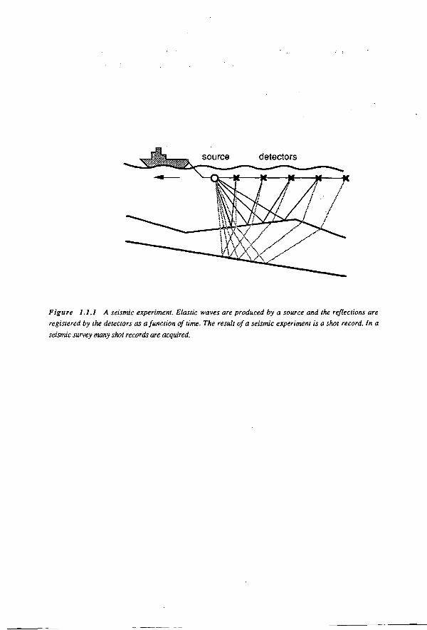
Figure 1.1.1 A seismic experiment. Elastic waves are produced by a source and the reflections are registered by the detectors as a function of time. The result of a seismic experiment is a shot record. In a seismic survey many shot records are acquired.
CHAPTER 1
INTRODUCTION
1.1 INTRODUCTION
An image of the Earth's subsurface can be acquired by carrying out a seismic survey. In seismic exploration elastic waves are generated by a source at the surface. For acquisition on land the usual source is dynamite or a seismic vibrator. For a marine survey airguns are most commonly used. The waves are radiated into the subsurface. However, whenever changes in the medium parameters occur, part of the wave field reflects and propagates upwards to the surface. Here it is detected with a number of receivers which are either geophones in case of a land acquisition or hydrophones in case of a marine acquisition. Such a seismic experiment is illustrated in Fig. 1.1.1. In order to get a good quality image the experiment is repeated many times with the shot and the detectors located at different surface positions, such that an inhomogeneity is 'illuminated' from different directions. The result of each seismic experiment is a shot record. It consists of the registration of the reflected wave fields at each detector. The reflected signal is registered as a function of travel time and it contains both propagation (down- and upward) and reflection effects of the subsurface. However, the aim is a structural image of the subsurface from which the propagation effects have been removed. This means that the reflection amplitudes should be presented as a function of lateral position and depth. The method that removes the propagation effects and transforms a time registration (x,y,t domain) into a depth image (x,y,z domain) is called seismic migration. The resolution of a migrated result is always limited, due to the finite bandwidth of the registered signals. Therefore the outcome of a migration process is a bandlimited estimation of the reflectivity properties of the subsurface.
The amount of data of a 3D seismic survey is generally very large. In order to reduce the amount of data and at the same time improve the signal to noise (S/N) ratio, stacking techniques have been developed. In this chapter the concept of stacking is discussed and the (dis)advantages of seismic processing in the prestack vs. the poststack domain are mentioned. Also a historic overview of migration is given in which the emphasis is on the
2 1 INTRODUCTION
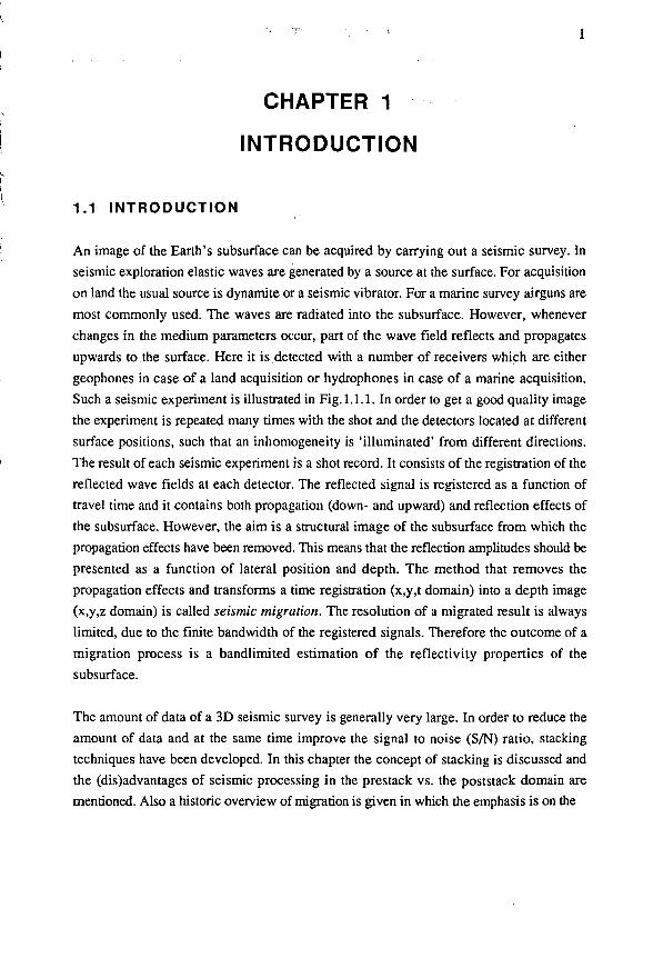
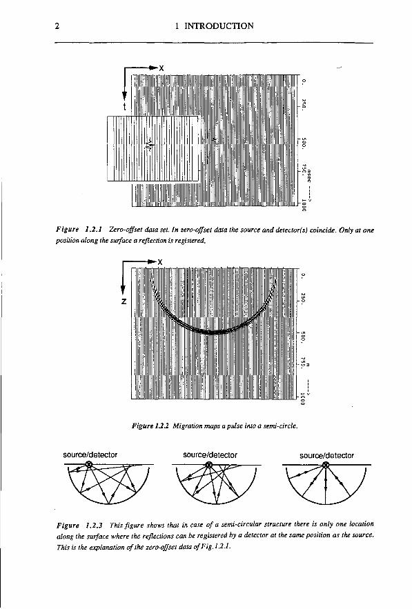
Figure 1.2.1 Zero-offset data set. In zero-offset data the source and detector(s) coincide. Only at one position along the surface a reflection is registered.
Figure 1.22 Migration maps a pulse into a semi-circle.
source/detector source/detector source/detector
Figure 1.2.3 This figure shows that in case of a semi-circular structure there is only one location along the surface where the reflections can be registered by a detector at the same position as the source. This is the explanation of the zero-offset data of Fig. 12.1.
1.2 GEOMETRICAL EXPLANATION OF ZERO-OFFSET MIGRATION 3
different methods that have been developed over the past. An overview of the TRITON*) philosophy on 3D processing is given next. Furthermore some practical aspects of 3D processing are discussed and finally an outline of this thesis is given. However, as a start, a simple geometrical explanation of zero-offset migration is presented.
1.2 GEOMETRICAL EXPLANATION OF ZERO-OFFSET MIGRATION
The distance between the source and a detector in a seismic experiment is called the offset. Hence, in a zero-offset configuration the source and detector(s) coincide. This situation can never be realized in a practical seismic survey due to the nature of the source. However, there are techniques that can be used to produce more or less accurate zero-offset data from nonzero-offset data. Such techniques are common midpoint (CMP) stacking, common reflection point (CRP) stacking and common depth point (CDP) stacking (see sections 1.3 and 1.4).
The concept of zero-offset migration is now explained with some examples.
Example 1: the migration impulse response. Consider the following situation. Zero-offset data are collected along a line at the surface (2D experiment). The recording shows that only at one surface location a reflected signal is measured; the zero-offset data set is shown in Fig. 1.2.1. Note that the data is a function of the lateral coordinate x and time t. A geologist can do little with the information the way it is presented here: it is not clear from which direction(s) the reflected energy has arrived at the detector nor is it obvious at what depth the reflectivity is located. If the velocity of wave propagation is known to be a certain constant, a migration of the zero-offset section would result in the depth section shown in Fig. 1.2.2. Zero-offset migration actually maps a pulse into a semi-circle (also called 'migration smile'). From Fig. 1.2.3 it should be clear that indeed a structure with a semicircular shape causes the zero-offset response of Fig. 1.2.1. Note that the migrated section of Fig. 1.2.2 is the 2D impulse response of the migration algorithm.
TRITON represents an international consortium on migration research, carried out at the Laboratory of Seismics and Acoustics at the Delft University of Technology.
4 1 INTRODUCTION
sources/detectors
point-diffractor
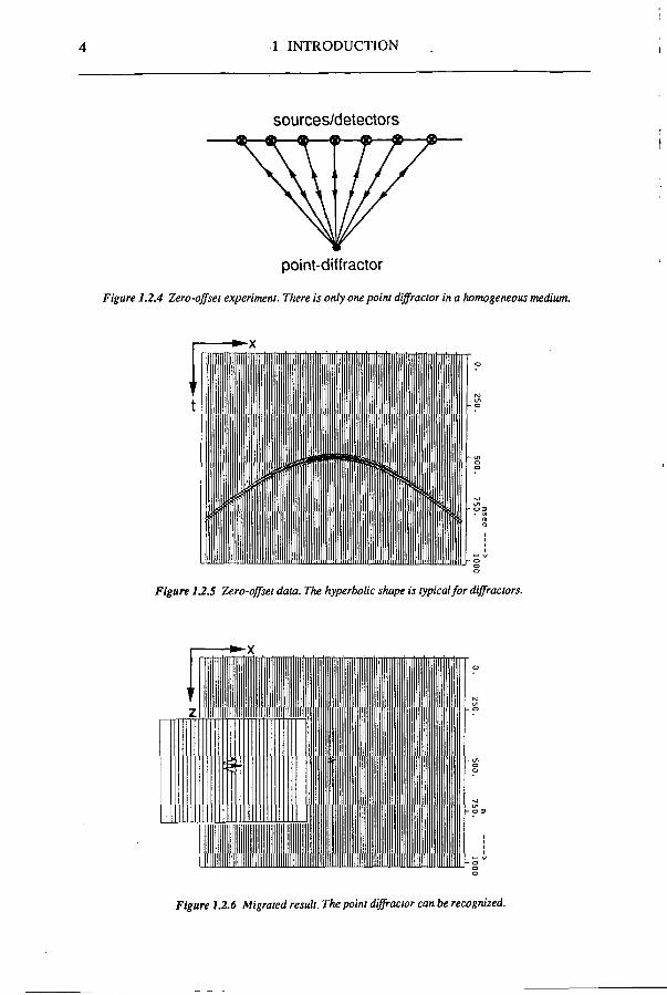
Figure 1.2.4 Zero-offset experiment. There is only one point diffraclor in a homogeneous medium.
Figure UJ Zero-offset data. The hyperbolic shape is typical for diffractors.
Figure 1.2.6 Migrated result. The point diffractor can be recognized.
1.2 GEOMETRICAL EXPLANATION OF ZERO-OFFSET MIGRATION 5
Example 2: the diffraction hyperbola. It is also interesting to investigate the situation of a single point diffractor in a homogeneous medium. The zero-offset experiment is illustrated
t in Fig. 1.2.4 and the zero-offset data can be seen in Fig. 1.2.5. The hyperbolic shape of the response is typical for diffractions. Migration should result in a reflectivity map of the subsurface. The result can be seen in Fig. 1.2.6. Indeed one can recognize the point diffractor: the diffracted energy has focussed well. From this example it follows that migration can be considered as the method that collapses the energy along a diffraction hyperbola to its apex.
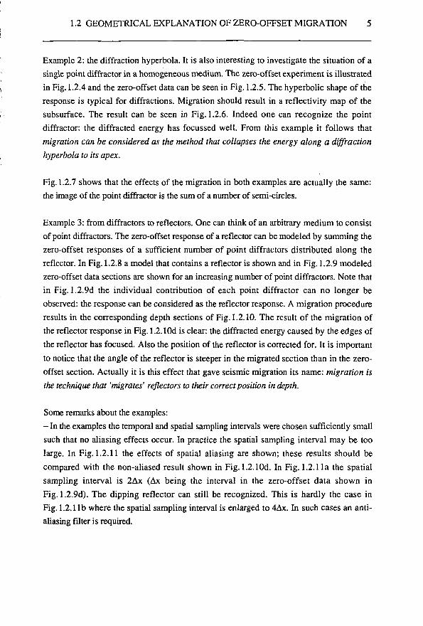
Fig. 1.2.7 shows that the effects of the migration in both examples are actually the same: the image of the point diffractor is the sum of a number of semi-circles.
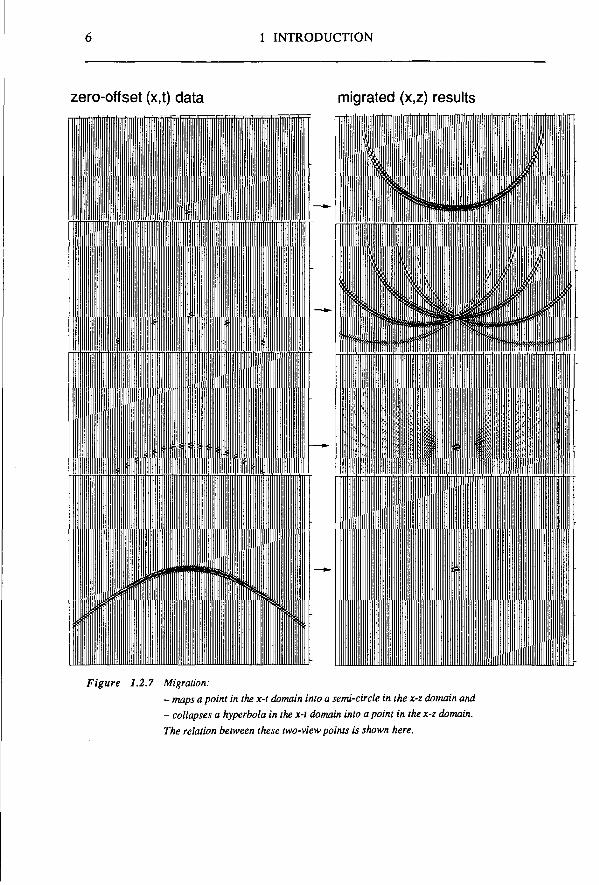
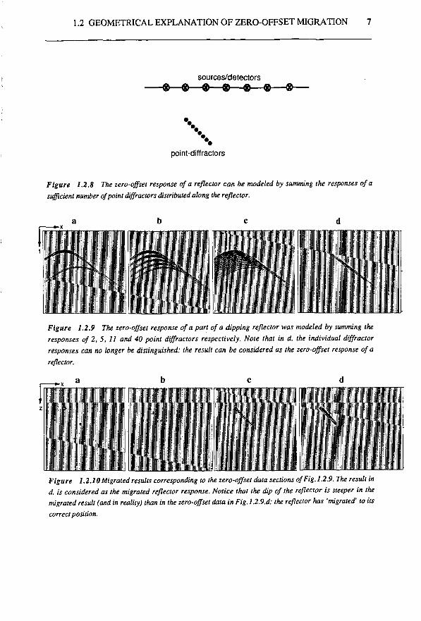
Example 3: from diffractors to reflectors. One can think of an arbitrary medium to consist of point diffractors. The zero-offset response of a reflector can be modeled by summing the zero-offset responses of a sufficient number of point diffractors distributed along the reflector. In Fig. 1.2.8 a model that contains a reflector is shown and in Fig. 1.2.9 modeled zero-offset data sections are shown for an increasing number of point diffractors. Note that in Fig. 1.2.9d the individual contribution of each point diffractor can no longer be observed: the response can be considered as the reflector response. A migration procedure results in the corresponding depth sections of Fig. 1.2.10. The result of the migration of the reflector response in Fig. 1.2.10d is clear: the diffracted energy caused by the edges of the reflector has focused. Also the position of the reflector is corrected for. It is important to notice that the angle of the reflector is steeper in the migrated section than in the zero-offset section. Actually it is this effect that gave seismic migration its name: migration is the technique that 'migrates' reflectors to their correct position in depth.
Some remarks about the examples: - In the examples the temporal and spatial sampling intervals were chosen sufficiently small such that no aliasing effects occur. In practice the spatial sampling interval may be too large. In Fig. 1.2.11 the effects of spatial aliasing are shown; these results should be compared with the non-aliased result shown in Fig. 1.2.10d. In Fig. 1.2.11a the spatial sampling interval is 2Ax (Ax being the interval in the zero-offset data shown in Fig. 1.2.9d). The dipping reflector can still be recognized. This is hardly the case in Fig. 1.2.11b where the spatial sampling interval is enlarged to 4Ax. In such cases an antialiasing filter is required.
6 1 INTRODUCTION
zero-offset (x,t) data migrated (x,z) results
Figure 1.2.7 Migration: - maps a point in the x-t domain into a semi-circle in the x-z domain and - collapses a hyperbola in the x-t domain into a point in the x-z domain. The relation between these two-view points is shown here.
1.2 GEOMETRICAL EXPLANATION OF ZERO-OFFSET MIGRATION 7
Figure 1.2.8 The zero-offset response of a reflector can be modeled by summing the responses of a sufficient number of point diffractors distributed along the reflector.
Figure 1.2.9 The zero-offset response of a part of a dipping reflector was modeled by summing the responses of 2, 5, 11 and 40 point diffractors respectively. Note that in d. the individual diffractor responses can no longer be distinguished: the result can be considered as the zero-offset response of a reflector.
_ ^ v a b c d
\
Figure 1.2.10 Migrated results corresponding to the zero-offset data sections of Fig. 1.2.9. The result in d. is considered as the migrated reflector response. Notice that the dip of the reflector is steeper in the migrated result (and in reality) than in the zero-offset data in Fig. 1.2.9.d: the reflector has 'migrated' to its correct position.
8 1 INTRODUCTION
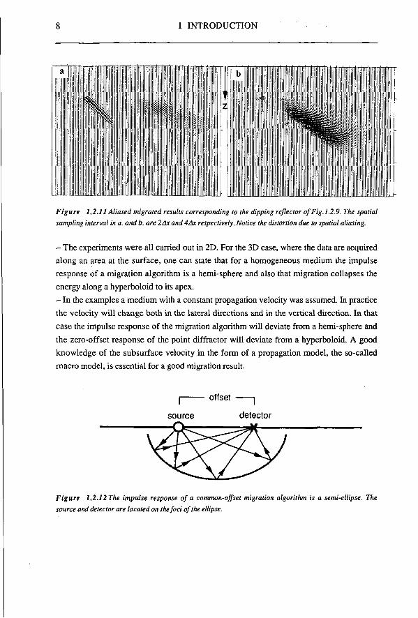
Figure 1.2.11 Aliased migrated results corresponding to the dipping reflector of Fig.1.2.9. The spatial sampling interval in a. and b. are 2Ax and 4 Ax respectively. Notice the distortion due to spatial aliasing.
- The experiments were all carried out in 2D. For the 3D case, where the data are acquired along an area at the surface, one can state that for a homogeneous medium the impulse response of a migration algorithm is a hemi-sphere and also that migration collapses the energy along a hyperboloid to its apex. - In the examples a medium with a constant propagation velocity was assumed. In practice the velocity will change both in the lateral directions and in the vertical direction. In that case the impulse response of the migration algorithm will deviate from a hemi-sphere and the zero-offset response of the point diffractor will deviate from a hyperboloid. A good knowledge of the subsurface velocity in the form of a propagation model, the so-called macro model, is essential for a good migration result.
I offset 1
source detector
Figure 1.2.12 The impulse response of a common-offset migration algorithm is a semi-ellipse. The source and detector are located on the foci of the ellipse.
1.3 POSTSTACK VERSUS PRESTACK 9
- The zero-offset configuration is actually a special case of the more general common-offset configuration, where there is a constant distance between the source and the detector. In Fig. 1.2.12 it can be seen that for a homogeneous medium the impulse response of a common-offset migration algorithm is a semi-ellipse (or a semi-ellipsoid in the 3D case) of which the source and detector positions are the focus points. - The modeling and migration of zero-offset responses are generally based on the 'half velocity substitution' or 'exploding reflector model' (Loewenthal et al., 1976). According to the exploding reflector model diffractors and reflectors are considered as buried sources that start to transmit waves ('explode') at zero travel time. Furthermore the propagation velocity of the medium is considered as half the true propagation velocity. Note that the one-way travel times in the exploding reflector configuration (from the buried sources up to the receivers) are now equal to the two-way travel times in reality (from the sources at the surface down to the diffractors/reflectors and up to the receivers at the surface). The exploding reflector model is based on the assumption that the source waves and the reflected waves travel along a common path in the subsurface. Apart from rare situations, the data modeled according to the exploding reflector concept have a good similarity with true zero-offset data as far as traveltimes are concerned. Also the results of migration based on the exploding reflector model are generally satisfactory. However, it can be shown that the amplitudes are not correct when the exploding reflector concept is used (Berkhout, 1985).
1.3 POSTSTACK VERSUS PRESTACK
In a seismic experiment the reflections of each shot are registered by a number of detectors (typically 96 per 2D shot record and 240 per 3D shot record). Stacking techniques have been developed in order to improve the S/N ratio and to reduce the amount of data. The so-called poststack data that result from these techniques are considered as zero-offset data. Hence, zero-offset techniques can be used for the migration of stacked data. Data reduction by conventional stacking techniques also means loss of information, e.g. the resolution is not optimum, from poststack data it is impossible to recover the angle dependent reflectivity etc. Contractors in the seismic industry therefore also offer prestack processing. In practice, prestack processing is limited to the 2D case. The amount of data acquired in a 3D survey - where not only the number of detectors per shot but also the number of shots is much larger than in a 2D survey - is in the order of Gbytes. Such a
10 1 INTRODUCTION
■*- offset
near offsets far offsets
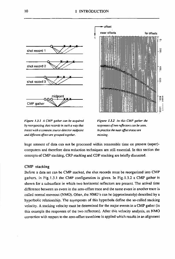
Figure 1.3.1 A CMP gather can be acquired Figure 1.3.2 In this CMP gather the by reorganizing shot records in such a way that responses of two reflectors can be seen. traces with a common source-detector midpoint In practice the near offset traces are and different offsets are grouped together. missing.
huge amount of data can not be processed within reasonable time on present (supercomputers and therefore data reduction techniques are still essential. In this section the concepts of CMP stacking, CRP stacking and CDP stacking are briefly discussed.
CMP stacking Before a data set can be CMP stacked, the shot records must be reorganized into CMP gathers. In Fig. 1.3.1 the CMP configuration is given. In Fig. 1.3.2 a CMP gather is shown for a subsurface in which two horizontal reflectors are present. The arrival time difference between an event in the zero-offset trace and the same event in another trace is called normal moveout (NMO). Often, the NMO's can be (approximately) described by a hyperbolic relationship. The asymptotes of this hyperbola define the so-called stacking velocity. A stacking velocity must be determined for the major events in a CMP gather (in this example the responses of the two reflectors). After this velocity analysis, an NMO correction with respect to the zero-offset traveltime is applied which results in an alignment
1.3 POSTSTACK VERSUS PRESTACK 11
of the events in the CMP gather. The traces of the NMO corrected gather are then stacked, which yields one poststack trace with an improved S/N ratio. This trace is considered as a zero-offset trace at the position of the surface midpoint. In practice four problems occur: 1. One stacked event may represent information from different reflection points.
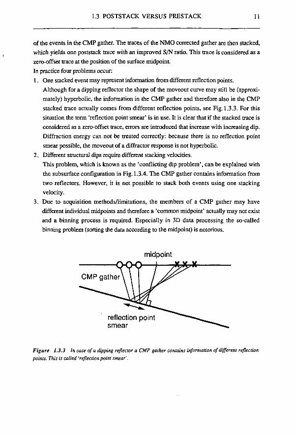
Although for a dipping reflector the shape of the moveout curve may still be (approximately) hyperbolic, the information in the CMP gather and therefore also in the CMP stacked trace actually comes from different reflection points, see Fig. 1.3.3. For this situation the term 'reflection point smear' is in use. It is clear that if the stacked trace is considered as a zero-offset trace, errors are introduced that increase with increasing dip. Diffraction energy can not be treated correctly: because there is no reflection point smear possible, the moveout of a diffractor response is not hyperbolic.
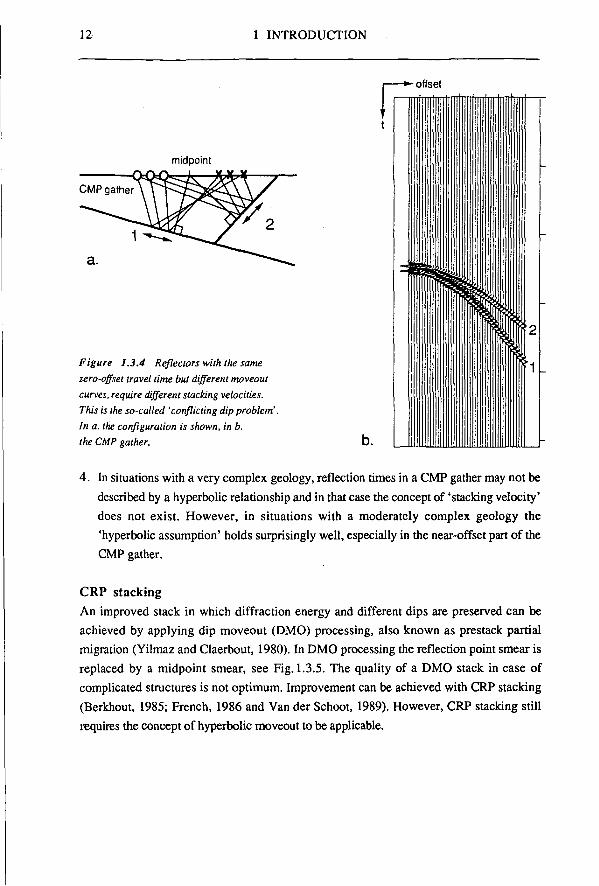
2. Different structural dips require different stacking velocities. This problem, which is known as the 'conflicting dip problem', can be explained with the subsurface configuration in Fig. 1.3.4. The CMP gather contains information from two reflectors. However, it is not possible to stack both events using one stacking velocity.
3. Due to acquisition methods/limitations, the members of a CMP gather may have different individual midpoints and therefore a 'common midpoint' actually may not exist and a binning process is required. Especially in 3D data processing the so-called binning problem (sorting the data according to the midpoint) is notorious.
midpoint
Figure 1.3.3 In case of a dipping reflector a CMP gather contains information of different reflection points. This is called 'reflectionpoint smear'.
12 1 INTRODUCTION
- offset
midpoint
Figure 1.3.4 Reflectors with the same zero-offset travel time but different moveout curves, require different stacking velocities. This is the so-called 'conflicting dip problem'. In a. the configuration is shown, in b. the CMP gather.
4. In situations with a very complex geology, reflection times in a CMP gather may not be described by a hyperbolic relationship and in that case the concept of 'stacking velocity' does not exist. However, in situations with a moderately complex geology the 'hyperbolic assumption' holds surprisingly well, especially in the near-offset part of the CMP gather.
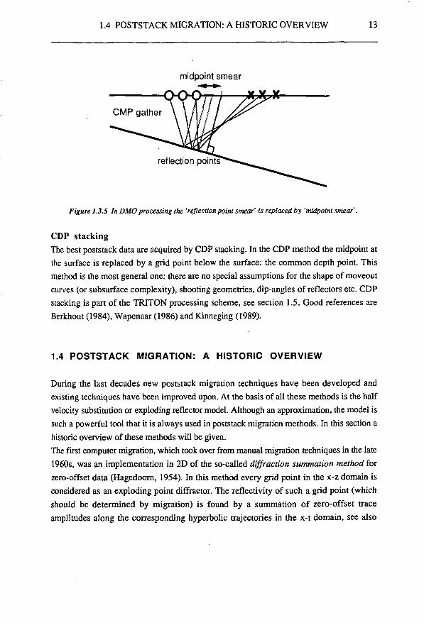
CRP stacking An improved stack in which diffraction energy and different dips are preserved can be achieved by applying dip moveout (DMO) processing, also known as prestack partial migration (Yilmaz and Claerbout, 1980). In DMO processing the reflection point smear is replaced by a midpoint smear, see Fig. 1.3.5. The quality of a DMO stack in case of complicated structures is not optimum. Improvement can be achieved with CRP stacking (Berkhout, 1985; French, 1986 and Van der Schoot, 1989). However, CRP stacking still requires the concept of hyperbolic moveout to be applicable.
1.4 POSTSTACK MIGRATION: A HISTORIC OVERVIEW 13
midpoint smear
CMP gather
reflection points
Figure 1.3.5 In DMO processing the 'reflection point smear' is replaced by 'midpoint smear'.
CDP stacking The best poststack data are acquired by CDP stacking. In the CDP method the midpoint at the surface is replaced by a grid point below the surface: the common depth point. This method is the most general one: there are no special assumptions for the shape of moveout curves (or subsurface complexity), shooting geometries, dip-angles of reflectors etc. CDP stacking is part of the TRITON processing scheme, see section 1.5. Good references are Berkhout (1984), Wapenaar (1986) and Kinneging (1989).
1.4 POSTSTACK MIGRATION: A HISTORIC OVERVIEW
During the last decades new poststack migration techniques have been developed and existing techniques have been improved upon. At the basis of all these methods is the half velocity substitution or exploding reflector model. Although an approximation, the model is such a powerful tool that it is always used in poststack migration methods. In this section a historic overview of these methods will be given. The first computer migration, which took over from manual migration techniques in the late 1960s, was an implementation in 2D of the so-called diffraction summation method for zero-offset data (Hagedoorn, 1954). In this method every grid point in the x-z domain is considered as an exploding point diffractor. The reflectivity of such a grid point (which should be determined by migration) is found by a summation of zero-offset trace amplitudes along the corresponding hyperbolic trajectories in the x-t domain, see also
14 1 INTRODUCTION
section 1.2 example 2. Obviously the method is based on the assumption that the zero-offset response of a point-diffractor is a hyperbola. However, this is true for a constant velocity medium only and approximately true for a horizontally layered medium in which case the rms velocity is used. In the presence of strong lateral velocity variations the hyperbolic assumption is no longer justified and the hyperbolic diffraction summation method will fail to produce correct results. It is interesting to mention that the method is purely based on geometrical arguments (ray theory) and not on wave theory. Properties that follow from wave theory and that are not taken into account by diffraction summation are: the spherical spreading in wave propagation, the directivity factor and the time differentiation factor, see also section 2.3. The low frequency appearance of early migration results can be explained by the neglection of the time differentiation factor. Improvements can be reached with the 'wave equation' migrations that have been developed later and that will be discussed next.
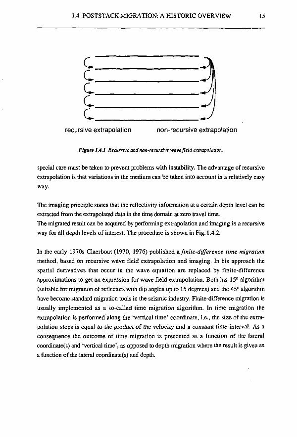
The majority of those migration methods is based on the one-way acoustic wave equation. According to the one-way approximation up- and downgoing wave fields can be treated independently. Because the exploding reflector model is assumed for zero-offset data, upgoing waves need to be considered only. Acoustic means that compressional waves are taken into account only and that shear waves are neglected. Most of the wave equation migration methods consist of the repeated application of two steps: wave field extrapolation and imaging. Wave field extrapolation techniques are used to downward continue data from one depth level, e.g. the surface, to a deeper level. Hence, wave field extrapolation makes it possible to transform surface data into data as they would have been recorded at an arbitrary depth level below the surface. In one-way extrapolation techniques a distinction is made between forward extrapolation and inverse extrapolation. In forward extrapolation the direction of wave propagation and the direction of extrapolation are the same; in inverse extrapolation the direction of wave propagation is opposite to the direction of extrapolation. In zero-offset migration the wave field extrapolation is of the inverse type: the extrapolation direction is downward whereas the waves propagate upwards. Wave field extrapolation techniques are either non-recursive or recursive. According to non-recursive extrapolation methods the wave fields at depth levels Z;, for i = 1 to N are all computed from the wave field at level ZQ', in recursive extrapolation the wave field at level z; is computed from the field at level Z;_i for i = 1 to N, see Fig. 1.4.1. Recursive extrapolation is sensitive to the accumulation of (small) errors that are involved in each extrapolation step. Therefore
1.4 POSTSTACK MIGRATION: A HISTORIC OVERVIEW 15
c c c c_ c
recursive extrapolation non-recursive extrapolation
Figure 1.4.1 Recursive and non-recursive wave field extrapolation.
special care must be taken to prevent problems with instability. The advantage of recursive extrapolation is that variations in the medium can be taken into account in a relatively easy way.
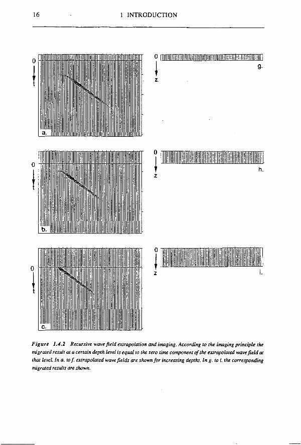
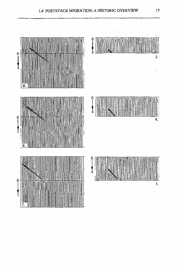
The imaging principle states that the reflectivity information at a certain depth level can be extracted from the extrapolated data in the time domain at zero travel time. The migrated result can be acquired by performing extrapolation and imaging in a recursive way for all depth levels of interest. The procedure is shown in Fig. 1.4.2.
In the early 1970s Claerbout (1970, 1976) published & finite-difference time migration method, based on recursive wave field extrapolation and imaging. In his approach the spatial derivatives that occur in the wave equation are replaced by finite-difference approximations to get an expression for wave field extrapolation. Both his 15° algorithm (suitable for migration of reflectors with dip angles up to 15 degrees) and the 45° algorithm have become standard migration tools in the seismic industry. Finite-difference migration is usually implemented as a so-called time migration algorithm. In time migration the extrapolation is performed along the 'vertical time' coordinate, i.e., the size of the extrapolation steps is equal to the product of the velocity and a constant time interval. As a consequence the outcome of time migration is presented as a function of the lateral coordinate(s) and 'vertical time', as opposed to depth migration where the result is given as a function of the lateral coordinate(s) and depth.
16 1 INTRODUCTION
ill liiill «11 l i B i l iiMJÉllli
I
Figure 1.4.2 Recursive wave field extrapolation and imaging. According to the imaging principle the migrated result at a certain depth level is equal to the zero time component of the extrapolated wave field at that level. In a. tof. extrapolated wave fields are shown for increasing depths. In g. to I. the corresponding migrated results are shown.
1.4 POSTSTACK MIGRATION: A HISTORIC OVERVIEW 17
d
Siil EMM
J-
1 e- HI
1 ii 1 1 1 ■ 1 1
1 m 1 liiiiiiHBan iiilii iiMiiiiiaiBiiiiiiiiiiiiiiiiSJiiiii11
| | j l
|
1 ill 1 1 1 1 1 II m
ll!f!!f!l!Miillli«HIIIfllfflllilffl
18 1 INTRODUCTION
Time migration is always implemented in such a way that it performs best in case of a laterally homogeneous medium. In section 2.1 extrapolation along the 'vertical time' coordinate is discussed in more detail.
Finite-difference migration is based on recursive extrapolation. This means that the errors involved in each extrapolation step will increase with depth. The errors due to the finite-difference approximation are frequency dependent which causes dispersion effects. Extension of the finite-difference method from 2D to 3D is not straightforward.
At the end of the 1970s a non-recursive migration method called Kirchhoff summation migration was presented by French (1975) and Schneider (1978). In this method, which is in principle suited for both 2D and 3D, extrapolation is based on the integral formulation of the solution of the scalar wave equation. Kirchhoff summation operators are hyperbolic. However, in Kirchhoff summation migration the spherical spreading, the directivity factor and the time differentiation factor are incorporated. This is the difference with diffraction summation. Berkhout and Van Wulfften Palthe (1979) introduced recursive Kirchhoff summation migration, in which vertical and lateral velocity variations can be handled in an efficient way because local velocities can be used. They also show that Kirchhoff summation operators can be seriously distorted by spatial operator aliasing, especially in case of the small extrapolation steps that occur in the recursive application. They explain that if the extrapolation step goes to zero (limit case), the Kirchhoff operator becomes a delta pulse and so, due to the infinite spatial bandwidth, this operator is seriously aliased. In chapter 3 of this thesis much attention is paid to the design of recursive Kirchhoff operators that are properly band-limited such that spatial operator aliasing is precluded.
The migration methods that have been mentioned so far are all implemented in the space-time domain. Another class is formed by the wavenumber-frequency domain migration techniques. Fourier transformation from the space-time to the wavenumber-frequency domain is a way to decompose an arbitrary wave field into monochromatic plane waves, each of which propagates in a unique direction. The extrapolation of a monochromatic plane wave is very simple: only a phase shift needs to be applied. This property was used by Gazdag (1978) for the design of a very efficient depth migration algorithm, called phase shift migration, based on recursive wave field extrapolation and imaging. There are in principle no errors involved in the extrapolation itself which means that the method is
1.4 POSTSTACK MIGRATION: A HISTORIC OVERVIEW 19
stable. Because of the recursive character of the migration, vertical velocity variations in die medium can be handled. However, lateral velocity variations can only be taken into account approximately if an extension of this method is used called phase shift plus interpolation (PSPI) (Gazdag and Squazzero, 1984). In this extension each recursive extrapolation step in which the wave field is downward continued from one depth level to the next is not performed once but several times with different constant velocities. This yields a number of extrapolated reference wave fields. The imaged result is then computed from the reference wave fields by interpolation in the space domain. Although depending on the complexity of the macro model, the number of reference wave fields to be computed is generally about five. This means that the PSPI method is also about five times less efficient than a simple phase shift migration. By far the fastest migration algorithm of today is the so-called Stolt f-k migration, (Stolt, 1978). The basis of this method is a procedure which maps the data from x,t to x,z in the double Fourier domain. The speed of the method is reached at the cost of the possibility of handling velocity variations correctly. To overcome this problem, Stolt suggested a time stretching procedure. Prior to migration the data are transformed such that they approximate the data that would have been recorded in case of a constant velocity subsurface. All migration methods in the wavenumber-frequency domain can be easily extended from 2D to 3D.
The best properties of migration methods in the space-time domain on the one hand and methods in the wavenumber-frequency domain on the other hand are combined in space frequency (x,co) migration as introduced by Berkhout (1980). Application of this method in three dimensions will be extensively discussed in this thesis.
A depth migration method that is not based on the principle of recursive extrapolation along the depth axis (or 'vertical time' axis in the case of time migration) is the so-called reverse-time migration (McMechan, 1983 and Baysal et al., 1983). In reverse-time migration the recursive extrapolation is performed backwards in time. Starting at the maximum registration time, the extrapolation is continued until time zero. During this process the zero-offset data are considered as boundary conditions at the surface. The extrapolation result at time zero is considered as the migrated section: all depths are then imaged simultaneously. The method is implemented in the space-time domain as a finite-difference solution of the two-way acoustic wave equation. The results are good; especially the high dip performance of the reverse-time migration is excellent. However, due to the finite-
20 1 INTRODUCTION
difference approximation of both the spatial and temporal derivatives, the method is very computationally intensive, which is a disadvantage for application in 3D (Chang and McMechan, 1989). In addition, the fact that all depth levels are imaged simultaneously at the last recursive step (zero time) is considered as a major drawback. 3D Processing has entered the seismic industry in the early 1980s. However, as is discussed in section 1.6, in many cases the existing 2D techniques are used in a 2 times 2D way to approximate full 3D processing. This is not correct for inhomogeneous media.
1.5 TRITON PHILOSOPHY ON 3D PROCESSING
According to the TRITON migration scheme (Berkhout et al., 1985) the 3D processing consists of the following steps: surface related pre-processing, prestack redatuming to the upper boundary of a target zone followed by CDP stacking and zero-offset migration within the target zone. The consecutive steps are now discussed.
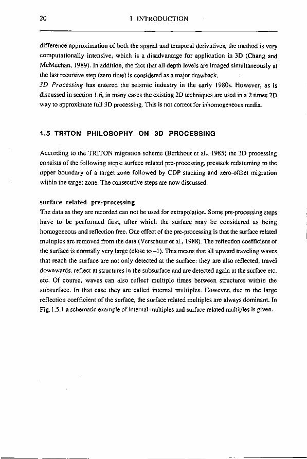
surface related pre-processing The data as they are recorded can not be used for extrapolation. Some pre-processing steps have to be performed first, after which the surface may be considered as being homogeneous and reflection free. One effect of the pre-processing is that the surface related multiples are removed from the data (Verschuur et al., 1988). The reflection coefficient of the surface is normally very large (close to -1). This means that all upward traveling waves that reach the surface are not only detected at the surface: they are also reflected, travel downwards, reflect at structures in the subsurface and are detected again at the surface etc. etc. Of course, waves can also reflect multiple times between structures within the subsurface. In that case they are called internal multiples. However, due to the large reflection coefficient of the surface, the surface related multiples are always dominant. In Fig. 1.5.1 a schematic example of internal multiples and surface related multiples is given.
1.5 TRITON PHILOSOPHY ON 3D PROCESSING 21
surface related multiples
internal multiples
Figure 1.5.1 Internal multiples and surface related multiples.
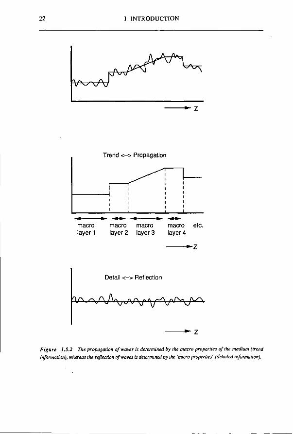
macro model versus detail Wave field extrapolation methods play a dominant role in the TRITON 3D processing scheme. They are used to compensate for the propagation effects of the medium. To do this properly a model containing the propagation properties of the medium is required. It turns out that wave propagation is determined by the macro parameters of the medium which represent the trend information of each major geological layer. The reflection of waves is determined by the 'micro' parameters of the medium which describe the fast changes in the medium: the deviations from the macro parameters, see Fig. 1.5.2. It seems contradictory that a macro model containing information about the medium is necessary prior to migration which has the purpose to collect this information. However, the required macro model only needs to contain the trend information in each macro layer, which is defined by the travel times. The detailed reflectivity information can then be found from the amplitudes by applying migration techniques.
redatuming to the upper boundary of the target zone Usually seismic interpreters are especially interested in a detailed map of the part of the subsurface where a reservoir might be present: the target zone. Hence, it is not necessary to do expensive processing on all the data in order to get a detailed map of the whole of the subsurface. An accurately detailed image of the target zone will be sufficient. The most important processing step in TRITON is redatuming. Shot records are extrapolated with a
22 1 INTRODUCTION
v^w -► z
Trend <-> Propagation
macro layer 1
macro layer 2
macro layer 3
macro layer 4
etc.
- ► Z
Detail <-> Reflection
V V ^ X A A V V A / V V - ^ V ^ V ^
Figure 1.5.2 The propagation of waves is determined by the macro properties of the medium (trend information), whereas the reflection of waves is determined by the 'micro properties' (detailed information).
1.5 TRITON PHILOSOPHY ON 3D PROCESSING 23
non-recursive generalized Kirchhoff technique from the acquisition surface to a new datum somewhere in the subsurface. This new datum can be the upper boundary of the target zone. After redatuming the shot records can be considered as if they had been acquired at the upper boundary of the target zone. The propagation properties of the overburden have been removed from the data by wave field extrapolation (redatuming), the propagation properties of the target zone are still in the data together with the reflectivity information. For a further discussion the reader is referred to Peels (1988) and Kinneging (1989).
construction of zero-offset data at the target boundary, CDP stack Redatuming also offers the possibility to construct other offsets at the upper boundary of the target than the offsets in the original shot records. This means that zero-offset data can be constructed. Unlike methods as CMP stacking or CRP stacking, which are based on hyperbolically shaped moveout curves, there are no such limitations when constructing zero-offset data after redatuming. Therefore this way of zero-offset data generation can be considered as a true CDP stacking method. The quality of the zero-offset data is generally excellent because high dip information is conserved as well as diffraction energy.
macro-model estimation/verification A good macro model is essential for the success of wave field extrapolation techniques such as redatuming and migration. An initial estimate of a macro model can be obtained from stacking velocities and picked travel times (Van der Made, 1988). In this case travel times in CMP gathers are used. However, due to the shortcomings of the CMP concept, see section 1.3, the estimated macro model may deviate from the true model, especially when the medium is complex. A better macro-model estimation technique is based on the examination of the consistency in CDP gathers. If the coherency in the CDP gathers is not optimum, this information is used to determine how the model should be changed in order to get an improved update. This process can be repeated iteratively which will converge to the desired result: an accurate macro model. In the TRITON project macro-model estimation is based on redatuming (Cox et al., 1988).
zero-offset migration within the target zone After redatuming with a good macro model, a high quality zero-offset data set is available at the upper boundary of the target zone. The size of this zero-offset data set is considerably smaller than the size of the prestack data before redatuming, which makes further full 3D processing feasible. As stated before, the redatuming has removed the propagation effects
24 1 INTRODUCTION
of the overburden. However, the propagation properties of the target zone are still included in the zero-offset data together with the reflectivity properties. To produce a good reflectivity map of the target zone from which the propagation effects have been removed, zero-offset migration can be applied. This zero-offset migration should be able to deal with complex macro models. Also it should not be limited in its ability to handle steeply dipping events. Such a 3D zero-offset migration is proposed in chapter 4.
1.6 2D VERSUS 3D
The use of 2D data acquisition and processing techniques is justified in areas where the medium parameters are a function of depth and one lateral direction only. Unfortunately
2D extrapolation x-direction
imaging
2D extrapolation x-direction
imaging
etc.
2D extrapolation ^-direction
imaging
2D extrapolation y-direction
3D extrapolation x- and y-direction
imaging
3D extrapolation x- and y-direction
imaging
etc.
imaging
etc.
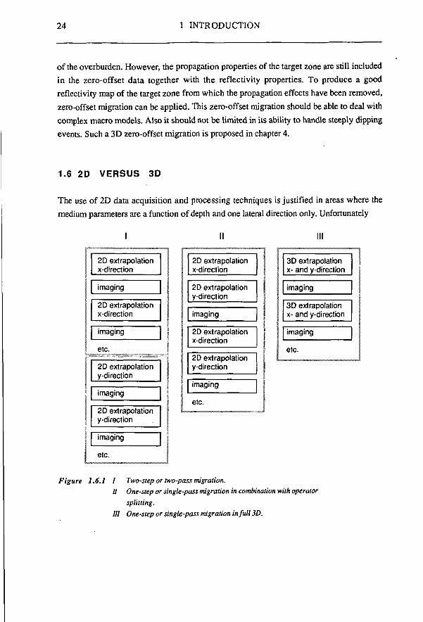
Figure 1.6.1 1 Two-step or two-pass migration. U One-step or single-pass migration in combination with operator
splitting. Ill One-step or single-pass migration in full 3D.
1.6 2D VERSUS 3D 25
such areas are not often found in practice. Since long it has been recognized that in case of a complex subsurface structure a 'hi-fi' image can only be achieved by using 3D techniques (French, 1975).
If the velocity variations in the medium are very small, such that a homogeneous macro model is a sufficient description of the propagation properties of the medium, 3D zero-offset migration can be carried out as a sequence of 2D zero-offset migrations (Gibson, Larner and Levin, 1983; and Jakubowicz and Levin, 1983). First, all 2D cross sections of the 3D zero-offset data in the x-direction are processed. Next, all 2D cross sections in the perpendicular y-direction are treated, see Fig. 1.6.1. This way of processing is called 'two-step' or 'two-pass' 3D migration. Its advantage is that all standard 2D migration algorithms can be used and that the method has in principle no dip limitations.
However, usually it is impossible to describe the propagation properties of the subsurface satisfactorily with a homogeneous macro model. Hence, two-step methods are not allowed in seismic exploration and 'one-step' or 'one-pass' 3D migration methods should be used instead. These are either approximately 3D, in case of operator splitting, or full 3D. Both types are now discussed.
If the reflected energy is not steeply dipping, a migration method can be used which is based on the concept of operator splitting. The principle of the method is recursive extrapolation and imaging. Each extrapolation step is performed as follows: first all 2D cross sections of the data in the x-direction are extrapolated using 2D operators; next all the 2D cross section in the y-direction of the result are extrapolated again with 2D operators, see Fig. 1.6.1. The problem is how to split a full 3D operator which depends on both x and y into independent 2D operators which depend on either x or y. It turns out that this operator splitting can only be done accurately in the small dip angle approximation (Ristow, 1980; Brown, 1983). Full 3D migration should be used in case of complex media where steeply dipping reflectors are present. This method is also based on recursive extrapolation and imaging. However, each extrapolation step is performed in a full 3D way, see Fig. 1.6.1.
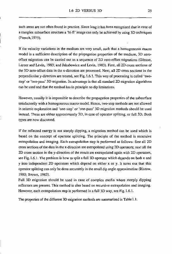
The properties of the different 3D migration methods are summarized in Table 1.1.
26 1 INTRODUCTION
Table 1.1 The properties of different 3D migration methods.
two-step
one-step operator splitting
one-step full 3D
steep dips
yes
no
yes
velocity variations
no
yes
yes
1.7 OUTLINE
Migration methods are based on wave field extrapolation. In chapter 2 of this thesis an inventory of wave field extrapolation techniques is presented. A choice is made for oneway acoustic wave field extrapolation in the space frequency domain with recursive Kirchhoff operators. The design of these operators in which both their accuracy and their efficiency are central, is discussed in chapter 3. The application of the recursive Kirchhoff extrapolation operators in migration is the subject of chapter 4. One of these migration techniques, full 3D zero-offset migration, was implemented. The details of this implementation are given in chapter 5 and in chapter 6 examples and results of the 3D zero-offset migration algorithm are shown. Finally, in the appendix, the application of the recursive Kirchhoff operators in 3D zero-offset modeling is discussed.
27
CHAPTER 2
AN INVENTORY OF WAVE FIELD EXTRAPOLATION TECHNIQUES IN
MIGRATION
2.1 INTRODUCTION
Wave field extrapolation is the key part of all migration techniques that are based on the wave equation. Most of the present techniques are based on the acoustic wave equation, i.e., compressional waves are taken into account only and shear waves are neglected. In this thesis we restrict ourselves to the acoustic case. A full elastic seismic processing scheme is developed in the DELPHI*) project (Berkhout and Wapenaar, 1988). In the introduction of this chapter we start with expressions for the one-way and two-way acoustic wave equation. The role of the Taylor series expansion in wave field extrapolation is shown. The Taylor series expansion is also used in the derivation of finite-difference expressions. This is illustrated with some examples. Next, the properties of a number of 3D acoustic wave field extrapolation methods are discussed. The are classified according to the coordinate along which the extrapolation is performed: - time, - depth, or - 'vertical time'. Furthermore, the methods can be characterized by the domain in which the extrapolation is performed: - space-time domain, - space-frequency domain, or - wavenumber-frequency domain and by the numerical technique that is used: - recursive explicit, - recursive implicit,
* DELPHI represents an international research consortium at the Laboratory of Seismics and Acoustics at the Delft University of Technology.
28 2. AN INVENTORY OF WAVE HELD EXTRAPOLATION TECHNIQUES
wave field extrapolation
c = c(x,y>z) d 0 r ™ n c = c(z)
f —) space-time space-frequency wavenumber-freqüêncy
extrapolation coordinate used in depth migration
f used in time migration
time depth 'vertical time'
technique
\ recursive non-recursive
explicit implicit hyperbolic non-hyperbolic
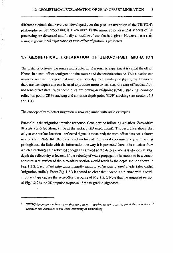
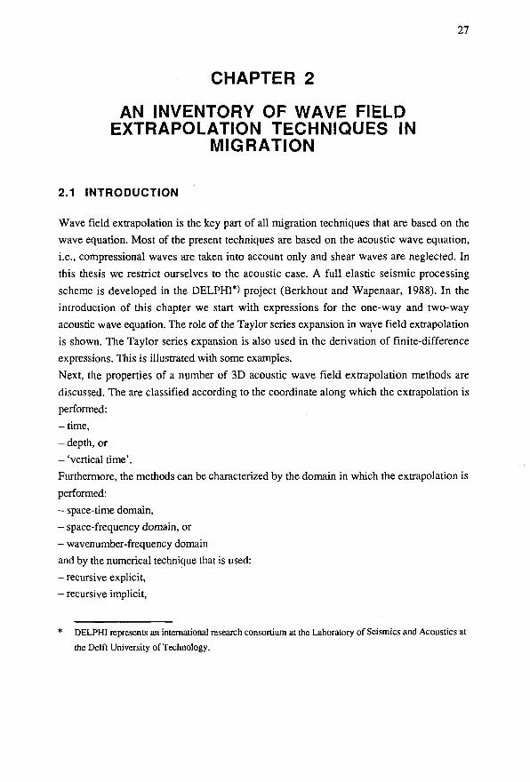
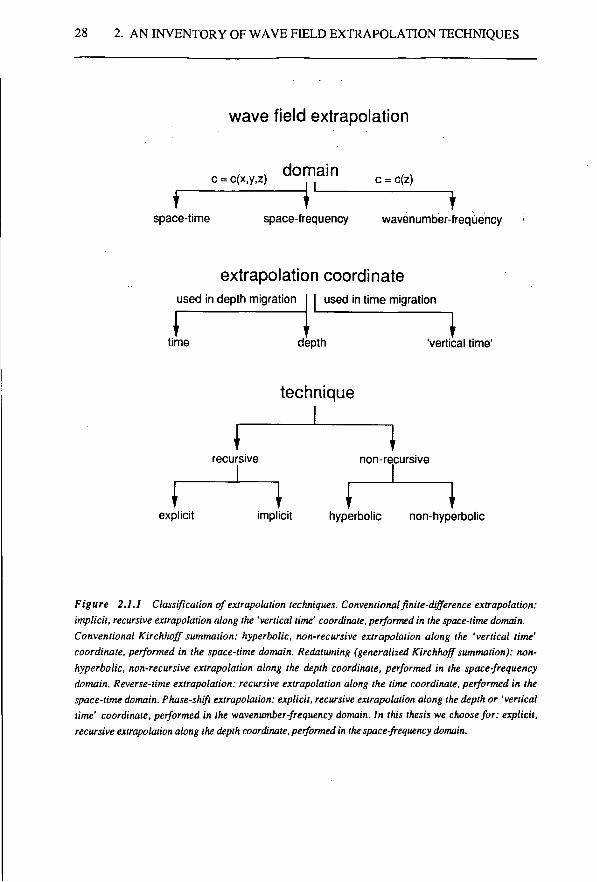
Figure 2.1.1 Classification of extrapolation techniques. Conventional finite-difference extrapolation: implicit, recursive extrapolation along the 'vertical time' coordinate, performed in the space-time domain. Conventional Kirchhoff summation: hyperbolic, non-recursive extrapolation along the 'vertical time' coordinate, performed in the space-time domain. Redatuming (generalized Kirchhoff summation): non-hyperbolic, non-recursive extrapolation along the depth coordinate, performed in the space-frequency domain. Reverse-time extrapolation: recursive extrapolation along the time coordinate, performed in the space-time domain. Phase-shift extrapolation: explicit, recursive extrapolation along the depth or 'vertical time' coordinate, performed in the wavenumber-frequency domain. In this thesis we choose for: explicit, recursive extrapolation along the depth coordinate, performed in the space-frequency domain.
2.1 INTRODUCTION 29
- non-recursive hyperbolic, or - non-recursive non-hyperbolic. This classification is also shown in Fig. 2.1.1. For migration, a choice is made for recursive explicit depth extrapolation. In the next sections the focus is on extrapolation methods of this type. Aspects that are included concern the flexibility of the method with respect to velocity variations in the medium, its robustness, the domain in which the extrapolation is performed, the implementation etc.
Acoustic wave equation The extrapolation techniques discussed in this chapter have in common that they are based on the acoustic wave equation. For an inhomogeneous fluid without losses and without sources, the linearized equation of motion and the linearized equation of continuity are given by
and r ? — a r (2-i}
KV.v = - | (2.2)
respectively. Here p = p(x,y,z,t) represents the acoustic pressure,
v = v(x,y,z,t) represents the particle velocity, p = p(x,y,z) represents the mass density, K = K(x,y,z) represents the adiabatic compression modulus, x, y and z represent the Cartesian coordinates (positive z-values correspond to
the downward direction) and t represents time.
Elimination of the particle velocity by substitution of eq. (2.2) in eq.(2.1), yields an expression for the two-way wave equation for acoustic pressure
V.( i V P ) = l f E - . (2.3) p K dt2
If the gradient of p may be neglected, eq. (2.3) can be written as
V 2 P = ^ , (2.4) c2 3t2
where c = c(x,y,z) = VK/p represents the wave propagation velocity. Note that the
30 2. AN INVENTORY OF WAVE HELD EXTRAPOLATION TECHNIQUES
influence of the density has not disappeared from wave equation (2.4) altogether: the contribution of the density is still included in the propagation velocity.
The equations given so far are formulated in the space-time domain. With Fourier techniques it is possible to perform transformations from the time domain to the frequency domain and/or from the space domain to the wavenumber domain and vice versa. In this thesis, the following definitions apply to the Fourier transformations: - The forward temporal Fourier transform of a real function g(x,y,z,t) from the time domain to the frequency domain is defined as
G(x,y,z,co) = f g(x,y,z,t) e ^ ' dt. (2.5) J—oo
Note that G(x,y,z,-co) = G*(x,y,z,co) because g(x,y,z,t) is real. This property is used in the definition of the inverse transformation. - The inverse temporal Fourier transformation is defined as
g(x,y,z,t) = ^ Real r Jo
G(x,y,z,co) e+J™ da> (2.6)
Here co represents the circular frequency. Note that only positive frequencies appear in eq. (2.6). The temporal Fourier transform of a function is indicated with a capital. -The double forward spatial Fourier transformation from the space domain to the wavenumber domain is defined as
G(kx,ky,z,co)= j j G(x,y,z,co)e+Jk'xe+Jk'>'dxdy. (2.7)
- The double inverse spatial Fourier transformation is defined as
G(x,y,z,Cö)=j—j \\ G(kx,ky,z,co) e-Jk"x e-Jkxy dkxdky. (2.8)
The spatial Fourier transform of a function is indicated by the symbol ~. If G satisfies the wave equation, kx and ky represent the x- and y-component of the wave vector k. A Fourier transformation from the space-time domain to the wavenumber-frequency domain of the wave field registered at the surface is a way to decompose the wave field into monochromatic plane waves, each of which travels in the direction defined by wave vector k.
2.1 INTRODUCTION 31
An additional Fourier transformation with respect to z can be defined in a similar way. - The forward spatial Fourier transformation with respect to z is given by
G(kx,ky>kz,(ö) = I G(kx,ky,z,co) e+i** dz . (2.9) J-oo
- The inverse spatial Fourier transformation with respect to z is given by
G(kx,ky,z,co) = — f Ö(kx,ky,kz,co) e"** dkz . (2.10) 27t/-~
Here kz represents the z-component of the wave vector k. The triple spatial Fourier transform is indicated by the symbol ~.
From the Fourier integrals the following properties with respect to differentiation can be derived. - Differentiation with respect to time, d/dt, is equivalent to multiplication by +jco in the frequency domain
3/3t<->+jo>. (2.11a) - Similarly: differentiation with respect to the spatial coordinates, 3/3x, d/dy and d/dz, is equivalent to multiplication by -jkx, -jky and -jkz respectively in the wavenumber domain
3/3x <-» -jkx, a/3y<->-jkyi (2.11b) d/dz <-> -fa.
Eq. (2.4) can be rewritten as
d P -, d P , d P i a P = 0 , 2 - . 2 - . 2 2 2 3x dy dz c 3t (2.12a)
The equivalent expression in the space-frequency domain is
dx dy ^ (2.12b)
32 2. AN INVENTORY OF WAVE HELD EXTRAPOLATION TECHNIQUES
where k = k(x,y,z) = co/c(x,y,z), and in the wavenumber-frequency domain
0- + (k*-l4-kj)p = O. (2.12c)
Here k = k(z) = co/c(z). The well known dispersion relation can be found by performing a spatial Fourier transformation with respect to z as well
k 2 - k * - k j - k * = 0. (2.12d)
In this equation k = co/c, with c constant.
The expressions (2.12) are the basis of various wave field extrapolation techniques.
Taylor series expansion The well known Taylor formula for series expansion can be used to derive an expression for wave field extrapolation. E.g., extrapolation along the time coordinate can be written as
p(t)=p(t„) + — ^ + ^ r ^ r + ~^r^ + ■■■ ( 2-1 3 )
This equation states that the pressure field at any time t can be computed from the pressure field and its derivatives towards t at time t„. The Taylor series expansion of the exponential function
exp(x) = l + f r + 2 7 + ^ 7 + ■•• <2-14)
can be used to rewrite eq. (2.13) in a symbolic notation as
p(t)=exp[(t-tn)^-]p(tn). (2.15) Otn
Substitution of t = tn+At, with At some positive time interval, yields
2.1 INTRODUCTION 33
p(tn±At) = exp(±At J - ) p(tn). (2.16)
The derivatives that occur in eq. (2.16) can be computed from the wave equation, e.g., for 3^/310^15 is simple: the expression follows directly from eq. (2.12a). The accuracy of the extrapolation depends on the number of terms that is included in the Taylor series, the extrapolation step size and the accuracy with which the derivatives are known. An expression similar to (2.15) can be derived for extrapolation along the depth coordinate, e.g.,
p(z) = exp[(z-z i)^-]p(Zi). (2.17)
According to eq. (2.17) the pressure field at any depth z can be computed from the pressure field and its derivatives towards z at depth level Zj.
The Taylor series approximation can also be used to derive finite-difference expressions for differentials. From the first order Taylor series expansion
pdn+AO-pdn) ± A t § - . (2.18) otn
the following much used finite-difference expressions for the first derivative can be derived:
|f- = [p(tn)-p(t„-At)] (2.19a)
and
|^~^[P( tn+At)-p( t n ) ] , (2.19b)
Addition of eq. (2.19a) and (2.19b) yields the following centered finite-difference expression for the first derivative
I t 1 " 2At [ p ( t n + A t ) ~ P ( t"-A t ) ] • (2-20)
34 2. AN INVENTORY OF WAVE HELD EXTRAPOLATION TECHNIQUES
The well known approximation for the second derivative
3t2 At2 [p(tn+At)-2p(tn) + p(tn-At)] (2.21)
can be found by substituting expression (2.19b) into the second order Taylor series expansion
p(t, :n-At) = p ( t n ) - A t è U ^ . dtn 2 at?
(2.22)
Finite-difference expressions similar to (2.19), (2.20) and (2.21) can be derived for d/dx, 32/3x2, d/dy, 32/3y2, 3/3z and 32/3z2.
Extrapolation along the time coordinate The expression for time extrapolation that is commonly used is formulated in the space-time domain. It is based on the second order Taylor series expansion
p(x,y,z,tn±At) = p(x,y,z,tn) ± At ^ + -^- -f . . otji -i 9t2
(2.23)
Substitution of finite-difference expression (2.19) for 3p/3t„ and using two-way wave equation (2.12a) for 3 ^ / 3 ^ yields
_ c2At2 p(x,y,z,tn±At) = 2p(x,y,z,t„) - p(x,y,z,tn+At) + —=—
3x2 3y2 3z2J ( (2.24)
Replacing the second derivatives towards x, y and z by finite-difference expressions as in eq. (2.21) yields the following discretized expression for reverse-time extrapolation (Chang and McMechan, 1989, andMcMechan, 1983)
Pk.l,m(tn±At) = 2 ( l -3a 2 ) Pk,l,m(tn) - Pk,l,m(tn+At) + (2.25)
+ a 2 (pk+l,l,m(tn) + Pk-Um(tn) + Pk,l+l,m(tn) + Pk,l-l,m(tn) + Pk.l,m+l(tn) + Pk,l,m-l(tn)) •
2.1 INTRODUCTION 35
Here pk,i,m(tn) is a shorthand notation for p(kAx,lAy,mAz,nAt), Ax = Ay = Az = h is the grid spacing and a = a(x,y,z) = cAt/h. (The same expression can also be found in a direct way by replacing the differentials in eq. (2.12a) by finite-difference approximations as in eq.(2.21)). Expression (2.25) states that in forward time extrapolation the wave field at time t+At is computed explicitly from the wave fields at times t and t-At. Similarly, in reverse time extrapolation the field at time t-At is computed from the fields at times t and t+At. Extrapolation along the time coordinate can be used in modeling (forward) as well as in migration (reverse). When used in zero-offset migration, the data provide the surface boundary conditions for the extrapolation: pk ] 0 (t^j). The reverse extrapolation is performed recursively from the final registration time T to zero time. The wave fields at times T+At and T+2At (which are necessary to initialize the extrapolation) are taken zero. The extrapolated wave field at zero time is the migrated result: all depths are imaged simultaneously at the final extrapolation step. Note that this property makes reverse-time extrapolation unsuitable for redatuming.
To keep the grid dispersion, which is inherent in the finite-difference approximation, to an acceptable level, the number of grid points per dominant wave length -dominant should be about 10 to 20
A. , ^ dominant
20 ' (2.26) The maximum finite-difference time step is limited by the stability condition
c*3 (2.27) As long as these conditions are satisfied the results of reverse-time extrapolation are good. Especially the high dip performance is excellent. However, the large number of grid points and the large number of time steps that are necessary cause the reverse-time extrapolation process in migration to be computationally intensive. Also the required computer memory is large: preferably the entire data volumes at two consecutive times should be stored in core memory.
Reverse-time extrapolation according to eq. (2.25) is based on the two-way acoustic wave equation. This means that both up- and downgoing waves are extrapolated simultaneously. So, apart from primary waves also multiply reflected waves and transmission effects are taken into account. This property is an advantage if the extrapolation is used for modeling.
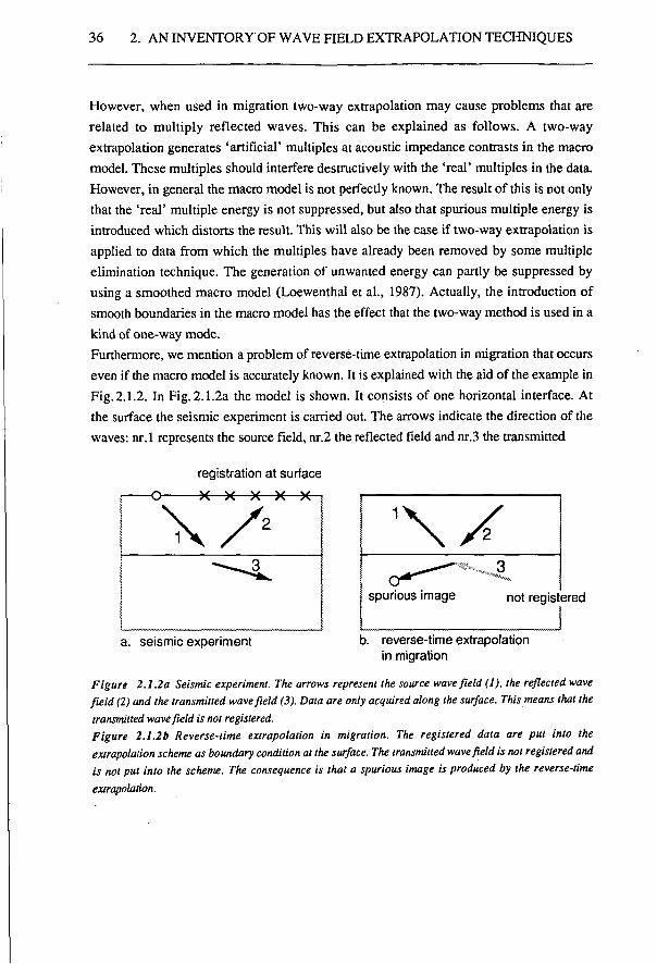
36 2. AN INVENTORY OF WAVE FIELD EXTRAPOLATION TECHNIQUES
However, when used in migration two-way extrapolation may cause problems that are related to multiply reflected waves. This can be explained as follows. A two-way extrapolation generates 'artificial' multiples at acoustic impedance contrasts in the macro model. These multiples should interfere destructively with the 'real' multiples in the data. However, in general the macro model is not perfectly known. The result of this is not only that the 'real' multiple energy is not suppressed, but also that spurious multiple energy is introduced which distorts the result. This will also be the case if two-way extrapolation is applied to data from which the multiples have already been removed by some multiple elimination technique. The generation of unwanted energy can partly be suppressed by using a smoothed macro model (Loewenthal et al., 1987). Actually, the introduction of smooth boundaries in the macro model has the effect that the two-way method is used in a kind of one-way mode. Furthermore, we mention a problem of reversé-time extrapolation in migration that occurs even if the macro model is accurately known. It is explained with the aid of the example in Fig. 2.1.2. In Fig. 2.1.2a the model is shown. It consists of one horizontal interface. At the surface the seismic experiment is carried out. The arrows indicate the direction of the waves: nr.1 represents the source field, nr.2 the reflected field and nr.3 the transmitted
registration at surface
a. seismic experiment
not registered
b. reverse-time extrapolation in migration
Figure 2.1.2a Seismic experiment. The arrows represent the source wave field (1). the reflected wave field (2) and the transmitted wave field (3). Data are only acquired along the surface. This means that the transmitted wave field is not registered. Figure 2.1.2b Reverse-time extrapolation in migration. The registered data are put into the extrapolation scheme as boundary condition at the surface. The transmitted wave field is not registered and is not put into the scheme. The consequence is that a spurious image is produced by the reverse-time extrapolation.
2.1 INTRODUCTION 37
field. Notice that only at the surface detectors have been placed. Hence, the transmitted field is not registered. However, it is required for a correct reconstruction. Therefore, reverse-time migration will not be able to give optimum results. Instead, it produces spurious images. This is illustrated in Fig. 2.1.2b where the spurious field is indicated by arrow nr.4. In order to get a perfect image of a certain area, the reflected and transmitted wave field should be known at a closed surface surrounding this area.
In an extrapolation scheme based on the one-way wave equation all reflections are considered as upgoing primary waves. This means that multiples and transmission effects are not handled correctly. However, no spurious energy is generated if an incorrect macro model is used. Because of this robustness we prefer one-way techniques in migration. The influence of multiples on the data should be reduced in advance, see section 1.5.
A reverse-time extrapolation technique based on the one-way wave equation was developed by Baysal et al. (1983) for the 2D case. To show the principle, we start with dispersion relation (2.12d):
w = W f e ) 2 + f e ) 2 + i • (2-28) or, with +jco <-» d/dt
The plus sign represents downgoing waves, whereas the minus sign corresponds to upgoing waves. This can be understood as follows. For clarity we consider waves that travel in the vertical direction only, i.e., kx = ky = 0. So, according to eq. (2.29) these waves are described by
^ ^ = ±jckzP(k2,t), (2.30)
or, with -jkz <-> d/dz
38 2. AN INVENTORY OF WAVE HELD EXTRAPOLATION TECHNIQUES
op(z,t) op(z,t) at + c 9z • (2-31)
Downgoing waves can be described by p+(ct-z): as time increases, depth increases as well, whereas upgoing waves are characterized by p~(ct+z): as time increases, depth decreases. From this it follows that downgoing waves satisfy
3 P ^ = _ C Ö P ^ 0 ( 2 3 2 at dz
and upgoing waves:
9j^!0= + c3pJz I0 ( 2 3 2 b ) dt dz
Note that the downward propagation in eq. (2.32a) corresponds to a plus sign in eq. (2.30). Equivalently, the upward propagation in eq. (2.32b) corresponds to a minus sign in eq.(2.30). We may extend this result to the more general case where the wave propagation has components in the x- and y-direction as well and we conclude that the plus sign in eq. (2.29) corresponds to downgoing waves whereas the minus sign in eq. (2.29) corresponds to upgoing waves. In reverse time zero-offset migration the extrapolation of upgoing waves plays an important role. Hence, we choose the minus sign in eq. (2.29):
a p - W z , t ) = _ j c k ^ | ^ 2 + | | 2 + i r ( k x k y k z t ) ( 2 3 3 )
The square root operator can not be expressed explicitly in the space domain and therefore it is computed in the wavenumber domain using forward and inverse triple spatial Fourier transformations (F and F~ ), (Gazdag, 1981). The expression for the one-way extrapolation is obtained from the centered finite-difference approximation of the time derivative, eq. (2.20)
Pw.m(tn±At) = p-k,,,m(t„-At) ± ^ - 2At, (2.34)
2.1 INTRODUCTION 39
or, with (2.33)
(2.35)
P"k.1,m(tn±At) = p-kil,m(tnTAt) + 2At cF-» [j k - V f e ) 2 + (fef+1 F [ p _ ( t n ) ] | k.,,m •
Apart from the fact that it is a one-way technique that can handle steep dips, reverse-time extrapolation according to eq. (2.35) has the advantage that numerical dispersion due to a finite-difference approximation of the spatial derivatives does not occur because these are computed in the wavenumber domain. However, the triple spatial Fourier transformations that are necessary in the 3D case at each extrapolation step, the large number of steps (small At) and the large memory requirements, cause this method to be unattractive from a computational point of view.
Extrapolation along the depth coordinate In recursive extrapolation along the depth coordinate, the extrapolation is performed with constant depth steps Az. According to eq. (2.17) depth extrapolation can be written as
p(x,y,z,t) = exp [(z-zik— ] p(x,y,Zi,t) .
Substitution of -jkz for 3/3z; (see (2.11)) yields the following expression in the wavenumber-frequency domain
P(kx,ky,z,CD) = exp [-jkz(z-zO ] P(kx,ky,Zi,co) , (2.36)
where, according to wave equation (2.12d), kz is defined as
kz = ±Vk2-ki-k£ for k2 + k2. S k2
and (2.37) kz = ±jVk2 + k 2 - k 2 fork2 + k2 > k2 .
Here k = co/c, with c constant. Note that nor the direction of the extrapolation, forward or inverse, nor the mode of
40 2. AN INVENTORY OF WAVE HELD EXTRAPOLATION TECHNIQUES
extrapolation, down- or upward, has yet been defined. E.g., in the next section we derive the following recursive expression for the inverse extrapolation of waves that propagate upwards:
P(kx,ky,zi+1,co) = F(kx,ky,Az,co) P(kx,ky,Zi,co) , with (2.38)
F(kx,ky,Az,co) = exp (jVk2-k?-k^ Az), for kj +ky- < k2 .
Here Az = z i + 1-z i , zi+1>Zi. Vertical velocity variations can be handled by adjusting the velocity at each extrapolation step. In section 2.2 wave field extrapolation in the wavenumber-frequency domain is treated in detail. It is argued that an implementation in this domain results in a very efficient scheme that has no dip limitation. However, in the wavenumber domain it is difficult to deal with lateral variations. If the extrapolation is performed in the space domain, the lateral variations can be handled. Recursive extrapolation along the depth coordinate in the space-frequency domain is discussed in section 2.3.
Wave field extrapolation according to eq. (2.38) is of the explicit type. An example of an implicit expression for extrapolation formulated in the wavenumber-frequency domain is
exp (-jkz — ) P(kx,ky,zi+1,co) = exp (+jkz — ) P(kx,ky,Zi,co) , (2.39)
or,
exp(+jkz — ) _ P(kx,ky,Zi+i,co) = -2— P(kx,ky,zi,co) . (2.40)
e x p ( - j k 2 y )
The advantage of an implicit formulation is that stable finite-difference schemes can be derived from it. Even if an approximation of the operator is used, its amplitude can always be defined such that it equals unity. This is because the numerator and the denominator of the operator in eq. (2.40) are complex conjugates. Of course, phase errors will be present in the approximation. Furthermore, implicit finite-difference schemes for the 3D case are complicated unless operator splitting techniques are used (Ristow,1980). Because we reject operator splitting in favor of full 3D operators, we prefer the explicit formulation. As we
2.1 INTRODUCTION 41
shall see in the next chapter, stable 3D wave field extrapolation operators can be designed for use in explicit schemes.
Non-recursive extrapolation along the depth coordinate can be performed either with hyperbolic operators or with non-hyperbolic operators, see Fig. 2.1.1. If hyperbolic operators are used (Kirchhoff summation) lateral velocity variations can not be handled correctly. Therefore a hyperbolic technique is rejected. Non-recursive depth extrapolation with non-hyperbolic operators (generalized Kirchhoff summation) would be the alternative. Note that such a method requires different extrapolation operators for every lateral position at each depth level. This is considered as a major disadvantage for application in migration where the extrapolation result at all depth levels is required (especially because a recursive extrapolation technique produces extrapolation results at all depth levels by necessity). However, for redatuming, where the extrapolation result is required at one depth level only, non-recursive non-hyperbolic depth extrapolation is pre-eminently suited. Therefore it is used in the TRITON scheme (Kinneging, 1989), see also section 1.5.
Extrapolation along the 'vertical time' coordinate T In recursive extrapolation along the 'vertical time' coordinate the extrapolation is performed with steps cAT, AT being constant. To arrive at an expression for extrapolation along the time coordinate we start with operator F as given in eq. (2.38):
F(kX)ky,Az,co) = eJ^k2- k* -ky Az . (2.41)
This expression can be rewritten as
F(kx,ky,Az,co) = eJkAz d (V^-k^-k2 . - k) Az t (2.42) or
F(kx>ky,Az,cu) = ejkAz eJkzAz . (2.43)
In migration schemes k is usually approximated by some series expansion (Taylor, continued fraction, etc.). It turns out that the expansion of ki converges better than the square root term in eq.(2.41). As mentioned, the steps in extrapolation along the time
42 2. AN INVENTORY OF WAVE FIELD EXTRAPOLATION TECHNIQUES
coordinate have the size cAT. This yields
F(kx,ky,AT,co) = eJk(cAT) eJk'z(cAT), or
F(kx,ky,AT,co) = eJöAT ejkz(cAT).
Notice that the first term in this equation is a simple time shift. We will now discuss three situations: 1. c = constant, 2. c = c(z)and 3. c = c(x,y,z).
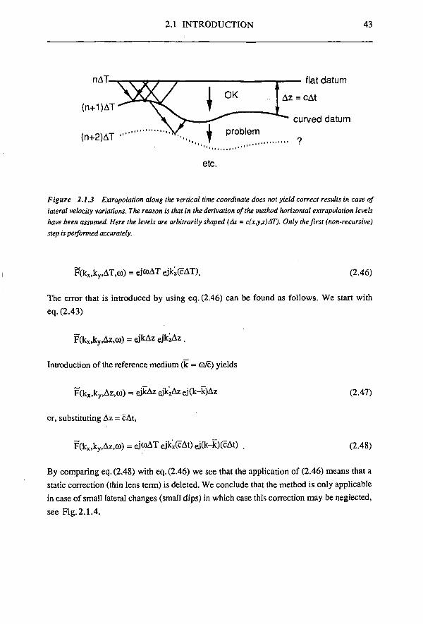
1. In case of a constant velocity medium, there is no difference between extrapolation along the depth coordinate and extrapolation along the 'vertical time' coordinate. This is because the step size in 'vertical time' extrapolation, cAt, is constant, like Az is constant in depth extrapolation. 2. If the velocity is a function of depth, c = c(z), the step size in 'vertical time' extrapolation is no longer constant.Therefore, in this case the time migrated result is a stretched version of the depth migrated result (or the other way around). Hence, use of time migration means that the vertical time to depth conversion is not carried out. 3. Problems arise if the velocity is a function of the spatial coordinates, c = c(x,y,z). In that case the step size in 'vertical time' extrapolation also varies with x, y and z. The effect is that the data are extrapolated to a dipping or even curved interface. The extrapolation method that is used however, is derived for extrapolation from a flat surface to some arbitrarily shaped surface. Therefore this method is only correct for non-recursive applications, starting at a flat datum. Hence, in a recursive application of extrapolation along the 'vertical time' coordinate, errors are involved if the velocity varies laterally. The situation is shown in Fig. 2.1.3. Those errors can be avoided by introducing a reference medium. In this medium the velocity is defined as some average of the true velocity such that it is a function of depth only: c = c(z), the overbar denotes the reference medium. The size of the extrapolation steps is defined as cAt. Hence, the following extrapolation operator is used (see also eq.(2.45)):
(2.44)
(2.45)
2.1 INTRODUCTION 43
nAT. - flat datum
etc.
Figure 2.1.3 Extrapolation along the vertical time coordinate does not yield correct results in case of lateral velocity variations. The reason is that in the derivation of the method horizontal extrapolation levels have been assumed. Here the levels are arbitrarily shaped (Az = c(x,y,z)AT). Only the first (non-recursive) step is performed accurately.
F(kx,ky,AT,co) = eJWAT eJki(cAT). (2.46)
The error that is introduced by using eq. (2.46) can be found as follows. We start with eq. (2.43)
F(kx,ky,Az,co) = ejkAz ejk'zAz .
Introduction of the reference medium (k = co/c) yields
F(kx,ky,Az,co) = eJkAzeJk'zAzej(k-k)Az
or, substituting Az = cAt,
F(kx,ky)Az,a)) = eJwAT ejkz(cAt) e)(k-k)(cAt) .
(2.47)
(2.48)
By comparing eq. (2.48) with eq. (2.46) we see that the application of (2.46) means that a static correction (thin lens term) is deleted. We conclude that the method is only applicable in case of small lateral changes (small dips) in which case this correction may be neglected, see Fig. 2.1.4.
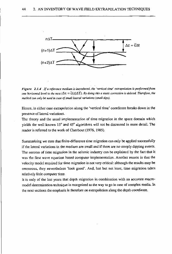
44 2. AN INVENTORY OF WAVE HELD EXTRAPOLATION TECHNIQUES
n A T -
(n+1)AT
(n+2)AT
Figure 2.1.4 If a reference medium is introduced, the 'vertical time' extrapolation is performed from one horizontal level to the next (Az = c(z)AT). By doing this a static correction is deleted. Therefore, the method can only be used in case of small lateral variations (small dips).
Hence, in either case extrapolation along the 'vertical time' coordinate breaks down in the presence of lateral variations. The theory and the usual implementation of time migration in the space domain which yields the well known 15° and 45° algorithms will not be discussed in more detail. The reader is referred to the work of Claerbout (1976,1985).
Summarizing we state that finite-difference time migration can only be applied successfully if the lateral variations in the medium are small and if there are no steeply dipping events. The success of time migration in the seismic industry can be explained by the fact that it was the first wave equation based computer implementation. Another reason is that the velocity model required for time migration is not very critical: although the results may be erroneous, they nevertheless 'look good'. And, last but not least, time migration takes relatively little computer time. It is only of the last years that depth migration in combination with an accurate macro-model determination technique is recognized as the way to go in case of complex media. In the next sections the emphasis is therefore on extrapolation along the depth coordinate.
Az = cAt
2.2 RECURSIVE DEPTH EXTRAPOLATION IN THE kx> ky, CO DOMAIN 45
2.2 RECURSIVE DEPTH EXTRAPOLATION IN THE kx, ky, co DOMAIN
The solution of wave equation (2.12c) is
P(kx,ky,z,co) = e±jVk2-kx-k3 | z;-z | p(kx,ky,Zi,co) for k2+k2 < k2 , (2.49a) and
P(kx,ky,z,co) = e±Vkl+k2-k2 | z;-z | P(kx,ky,Zi,co) for k^+k2 > k2 . (2.49b)
This well known result can be easily verified by substitution. The expressions for the forward extrapolation of upward traveling waves (z<z,) are found by choosing the minus sign in eq.(2.49)
P"(kX)ky>z,co) = e-jVk2-k2-k2 (z;-z) p-(kX)ky,Zj,co) for k2+k2 < k2 , (2.50a) and
P"(kx,ky,z,co) = e-Vki+k?-k2(zi-z) p-(kX)ky,Zj,cü) for k2+k2 > k2 . (2.50b)
The superscript_ denotes upward traveling waves. The part of the wave field for k2 + ky > k2 is generally referred to as the evanescent field. The minus sign in eq. (2.50b) is chosen on physical grounds: the evanescent waves decrease exponentially. Because of this property, the registration at the surface of reflected evanescent waves is below the noise level and therefore these waves can not be used.
Eq. (2.50) states that the upward traveling wave field at any depth in the subsurface above level z; can be computed from the field at level z;. Hence, recursive extrapolation can be expressed as
p-^.ky.Zj.Lü)) = W(kx,ky>Az,co) p-(kx,ky>Zi,co), (2.51)
where Az = Z; - Zj_j, zj > zj_i, and
W(kX)ky,Az,co) = e-jVk2-k2-k^ Az f o r k2+k2 ^ k2 > (2.52a) and
W(kx,ky,Az,co) = e-Vki+k^k2 Az f o r k2+k2 > k2 (2.52b)
46 2. AN INVENTORY OF WAVE HELD EXTRAPOLATION TECHNIQUES
In recursive wave field extrapolation vertical velocity variations can be taken into account, because at each extrapolation step a new velocity can be assumed. However, because of the double spatial Fourier transformation, lateral velocity variations can not be handled by extrapolation according to eq. (2.51). This however can be accomplished in the space domain, see the next section.
The inverse wave field extrapolation operator F is defined such that
P'(kx,ky,Zi,co) = F(kx,ky,Az,co) P-(kJ(,ky,Zi_1,co). (2.53)
Substitution of eq. (2.51) into eq. (2.53) yields
F(kx,ky,Az,co) W(kx,ky,Az,co) = 1 , (2.54) or,
F(kx,ky,Az,co) = W (kx,ky)Az,o)). (2.55)
Using eq. (2.52) F can be expressed as follows
F(kx,ky,Az,co) = e+jVk2-k2-ky Az f o r k2+k2 < k2 ; (2.56a) and
F(kx,ky,Az,(ü) = e-^ i+ky-k 2 ** for kx+k2 > k2 . (2.56b)
The practical application of eq. (2.56b) in the inverse wave field extrapolation of evanescent waves would cause stability problems. As mentioned, the S/N ratio in the registration of those waves is very small. Hence, the extrapolation would cause an exponential increase of the noise. Therefore, instead of eq. (2.55), the matched filter approach is often followed in practice
* F(kx,ky,Az,co) = W (kx,ky,Az,co), (2.57)
or, with eq. (2.52)
2.2 RECURSIVE DEPTH EXTRAPOLATION IN THE kx, ky, CO DOMAIN 47
F(kx,ky,Az,co) = e+jVk2-k2-k2 Az f o r k |+ k2 < k2 >
and
F(k ,ky,Az,co) = e-Vkl+ky-k2 Az f o r k2+k2 > k2 x>*-y
(2.58a)
(2.58b)
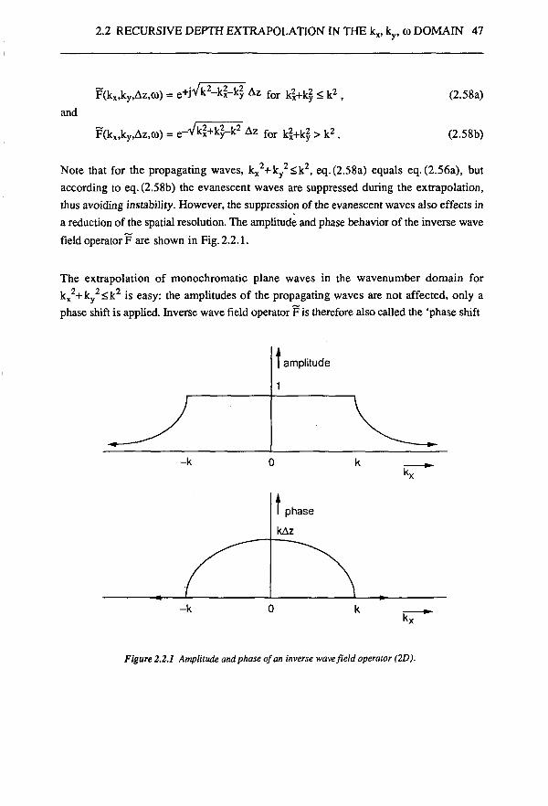
Note that for the propagating waves, kx2+ky
2<k2, eq.(2.58a) equals eq. (2.56a), but according to eq. (2.58b) the evanescent waves are suppressed during the extrapolation, thus avoiding instability. However, the suppression of the evanescent waves also effects in a reduction of the spatial resolution. The amplitude and phase behavior of the inverse wave field operator F are shown in Fig. 2.2.1.
The extrapolation of monochromatic plane waves in the wavenumber domain for kx
2+ky2<k2 is easy: the amplitudes of the propagating waves are not affected, only a
phase shift is applied. Inverse wave field operator F is therefore also called the 'phase shift
amplitude
1
kx
Figure 2.2.1 Amplitude and phase of an inverse wave field operator (2D).
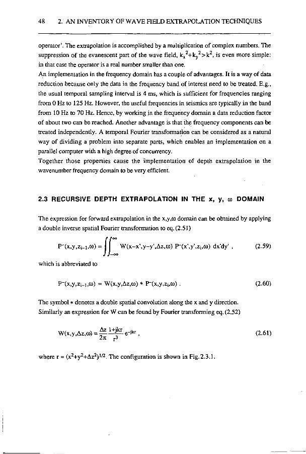
48 2. AN INVENTORY OF WAVE HELD EXTRAPOLATION TECHNIQUES
operator'. The extrapolation is accomplished by a multiplication of complex numbers. The suppression of the evanescent part of the wave field, kx
2+ky2>k2, is even more simple:
in that case the operator is a real number smaller than one. An implementation in the frequency domain has a couple of advantages. It is a way of data reduction because only the data in the frequency band of interest need to be treated. E.g., the usual temporal sampling interval is 4 ms, which is sufficient for frequencies ranging from 0 Hz to 125 Hz. However, the useful frequencies in seismics are typically in the band from 10 Hz to 70 Hz. Hence, by working in the frequency domain a data reduction factor of about two can be reached. Another advantage is that the frequency components can be treated independently. A temporal Fourier transformation can be considered as a natural way of dividing a problem into separate parts, which enables an implementation on a parallel computer with a high degree of concurrency. Together those properties cause the implementation of depth extrapolation in the wavenumber frequency domain to be very efficient.
2.3 RECURSIVE DEPTH EXTRAPOLATION IN THE x, y, co DOMAIN
The expression for forward extrapolation in the x,y,co domain can be obtained by applying a double inverse spatial Fourier transformation to eq. (2.51)
(x,y,zi_i,co) = I I P-(x,y,zi_i,co) = I | W(x-x',y-y',Az,u)) p-(x',y',Zi,co) dx'dy' , (2.59)
which is abbreviated to
P-Xx.y.ZM.co) = W(x,y,Az,co) * P-(x,y,Zi,co) . (2.60)
The symbol * denotes a double spatial convolution along the x and y direction. Similarly an expression for W can be found by Fourier transforming eq. (2.52)
W(x,y,Az,co) = ^ . 1 ^ - e-J^ , (2.61) Z7t j-3
where r = (x2+y2+Az2)1/2. The configuration is shown in Fig. 2.3.1.
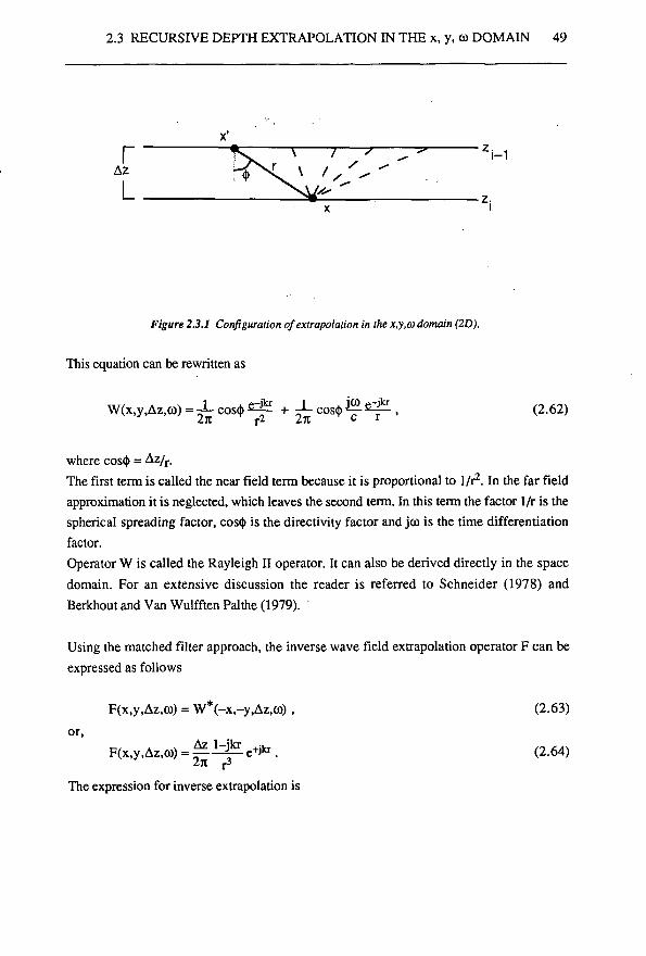
2.3 RECURSIVE DEPTH EXTRAPOLATION IN THE x, y, oo DOMAIN 49
Figure 23.1 Configuration of extrapolation in the x.y.co domain (2D).
This equation can be rewritten as
W(x,y)AZ>co) = - L cos* S-ÊL + X cos*&■ ±L , (2.62) Z7t r2 271 C r
where cos* = Az/r. The first term is called the near field term because it is proportional to 1/r2. In the far field approximation it is neglected, which leaves the second term. In this term the factor 1/r is the spherical spreading factor, cos* is the directivity factor and jco is the time differentiation factor. Operator W is called the Rayleigh n operator. It can also be derived directly in the space domain. For an extensive discussion the reader is referred to Schneider (1978) and Berkhout and Van Wulfften Palthe (1979).
Using the matched filter approach, the inverse wave field extrapolation operator F can be expressed as follows
F(x,y,Az,co) = W*(-x,-y,Az,co) , (2.63) or,
F(x,y,Az,co) = i ^ . e+J* . (2.64) 271 j3
The expression for inverse extrapolation is
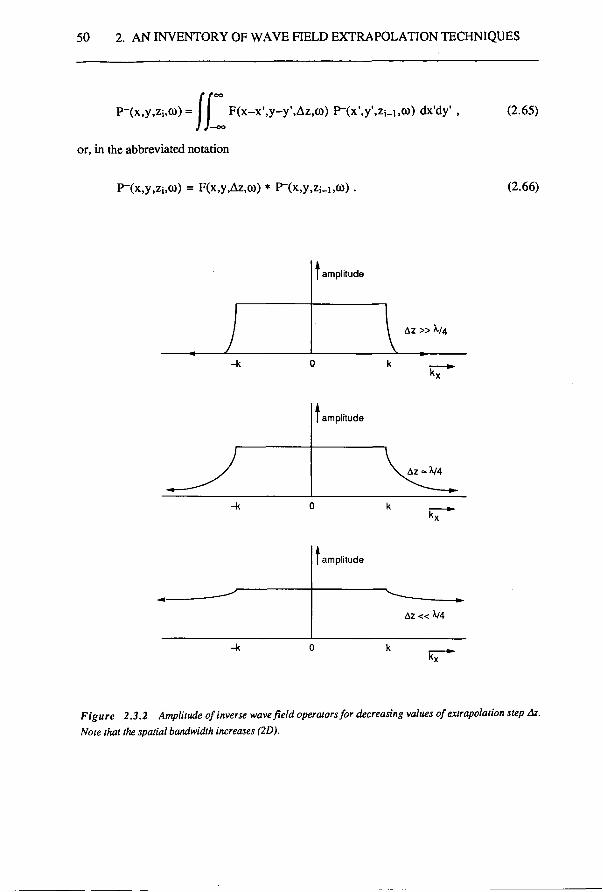
50 2. AN INVENTORY OF WAVE HELD EXTRAPOLATION TECHNIQUES
(x.y.zi.co) = I I p-(x,y,Zi,co) = | | FU-x'.y-y'.Az.co) P-(x\y',Zi_i,co) dx'dy', (2.65)
or, in the abbreviated notation
p-(x,y,Zi,co) = F(x,y,Az,co) * P-(x,y,Zi_i,co) (2.66)
| amplitude
Az » ^/4
I amplitude
Az = V4
[ amplitude
Az « V4
Figure 2.3.2 Amplitude of inverse wave field operators for decreasing values of extrapolation step Az. Note that the spatial bandwidth increases (2D).
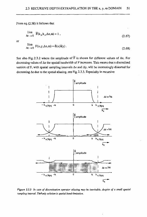
2.3 RECURSIVE DEPTH EXTRAPOLATION IN THE x, y, co DOMAIN 51
From eq. (2.58) it follows that
£™Q F(k„kx.Az,(D)=l.
or lim
Az-»0 F(x,y,Az,co) = 8(x)8(y).
(2.67)
(2.68)
See also Fig. 2.3.2 where the amplitude of F is shown for different values of Az. For decreasing values of Az the spatial bandwidth of F increases. This means that a discretized version of F, with spatial sampling intervals Ax and Ay, will be increasingly distorted for decreasing Az due to the spatial aliasing, see Fig. 2.3.3. Especially in recursive
amplitude
Az»>/4
1 x.Nyq - k k k x.Nyq
I amplitude
Az = V4
' ^x.Nyq ~^ k k x.Nyq
[amplitude
:Z_^J -A z « V 4
'x.Nyq k k x.Nyq
Figure 2.3.3 In case of discretization operator aliasing may be inevitable, despite of a small spatial sampling interval. The*only solution is spatial band-limitation.
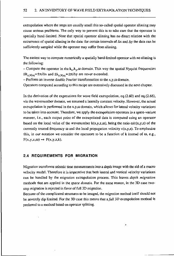
52 2. AN INVENTORY OF WAVE HELD EXTRAPOLATION TECHNIQUES
extrapolation where the steps are usually small this so-called spatial operator aliasing may cause serious problems. The only way to prevent this is to take care that the operator is spatially band-limited. Note that spatial operator aliasing has no direct relation with the occurrence of spatial aliasing in the data: for certain intervals of Ax and Ay the data can be sufficiently sampled while the operator may suffer from aliasing.
The easiest way to compute numerically a spatially band-limited operator with no aliasing is the following: - Compute the operator in the kx,ky)co domain. This way the spatial Nyquist frequencies ±kxNyq=±rc/Ax and ±kyNyq=±7i/Ay are never exceeded. - Perform an inverse double Fourier transformation to die x,y,co domain. Operators computed according to this recipe are extensively discussed in the next chapter.
In the derivation of the expressions for wave field extrapolation, eq.(2.60) and eq.(2.66), via the wavenumber domain, we assumed a laterally constant velocity. However, the actual extrapolation is performed in the x,y,co domain, which allows for lateral velocity variations to be taken into account. Therefore, we apply the extrapolation operators in a space-variant manner, i.e., each output point of the extrapolated data is computed using an operator based on the local value of the wavenumber k(x,y,z,co), being the ratio co/c(x,y,z) of the currently treated frequency co and the local propagation velocity c(x,y,z). To emphasize this, in our notation we consider the operators to be a function of k instead of co, e.g., F(x,y,z,to) -» F(x,y,z,k).
2.4 REQUIREMENTS FOR MIGRATION
Migration transforms seismic time measurements into a depth image with the aid of a macro velocity model. Therefore it is imperative that both lateral and vertical velocity variations can be handled by the migration extrapolation process. This leaves depth migration methods that are applied in the space domain. For the same reason, in the 3D case two-step migration is rejected in favor of full 3D migration. Because of the complicated structures to be imaged, the migration method itself should not be severely dip limited. For the 3D case this means that a full 3D extrapolation method is preferred to a method based on operator splitting.
2.4 REQUIREMENTS FOR MIGRATION 53
For reasons of efficiency the migration should is implemented as a poststack or zero-offset method. Also for reasons of efficiency migration in the frequency domain is chosen and not reverse-time migration. Because of its robustness a one-way extrapolation technique is considered best. Summarizing, above arguments lead to the following choice: 3D zero-offset depth migration based on recursive wave field extrapolation. The extrapolation should be oneway and full 3D; the implementation should be in the x,y,co domain.
Because of the recursive character of the extrapolation process the errors made in each extrapolation step should be made sufficiently small. This especially concerns the amplitude errors that may cause instability. To prevent operator aliasing, which is likely to occur in case of the small extrapolation steps, the extrapolation operators should be spatially band-limited.
In the next chapters attention is paid to the design of efficient, accurate extrapolation operators and to migration based on extrapolation with those operators.
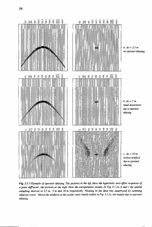
54
a. Ax = 25 m no operator aliasing
b. Ax = 5 m small distortions due to operator aliasing
c. Ax = 10 m serious artefacts due to operator
- aliasing
Fig. 3.1.1 Example of operator aliasing. The pictures at the left show the hyperbolic zero-offset responses of a point diffractor, the pictures at the right show the extrapolation results. In Fig. 3.1.1a, b and c the spatial sampling interval is 2.5 m, 5 m and 10 m respectively. Aliasing in the data was suppressed by summing adjacent traces . Hence the artefacts in the results, most clearly visible in Fig. 3.1.1c, are mainly due to operator aliasing.
55
CHAPTER 3
DESIGN OF ACCURATE EFFICIENT RECURSIVE KIRCHHOFF EXTRAPOLATION
OPERATORS
3.1 INTRODUCTION
In this chapter the design of recursive wave field extrapolation operators for application in the space-frequency domain is discussed. A high accuracy is very important: even small errors in the operators, e.g. in the order of one percent, will cause unacceptably large errors in the final result. This is because the errors accumulate due to the recursive application of the operators. One important source of errors, the use of operators that are spatially aliased, see Fig. 3.1.1, can be eliminated by computing the operators in the kx,k domain. If the operators are truncated in this domain such that the spatial Nyquist frequencies are not exceeded, an inverse spatial Fourier transformation to the x,y domain yields the desired non-aliased extrapolation operators. However, operators computed according to this recipe are not the most efficient, i.e., their application in the x,y domain is computationally intensive. Truncation of the operators in this domain (or, equivalently, reduction of the number of points) increases the efficiency. Unfortunately, truncation decreases the accuracy. This is because the shape of the operator in the kx,ky domain and the shape of the operator in the x,y domain are coupled. The larger
the derivatives with respect to kx or ky of operator F in the kx,ky domain, the larger the size of the equivalent operator F in the x,y domain domain should be. This property is demonstrated. Special attention is paid to small-sized operators that nevertheless have a good accuracy and stability: 'smoothed' operators and 'optimized' operators. The 'smoothed' operators are designed analytically in the kx,ky domain such that large derivatives are avoided. The 'optimized' operators are computed numerically by minimization of errors. Because an 'optimized' operator has the smallest possible size for a given accuracy, it can be considered as an optimally truncated one. Criteria are derived in the kx,ky domain for the maximum phase and amplitude errors that can be allowed. Furthermore, to increase the efficiency of the extrapolation process itself, the symmetry properties of the operators are used. By computing the operators in advance and storing
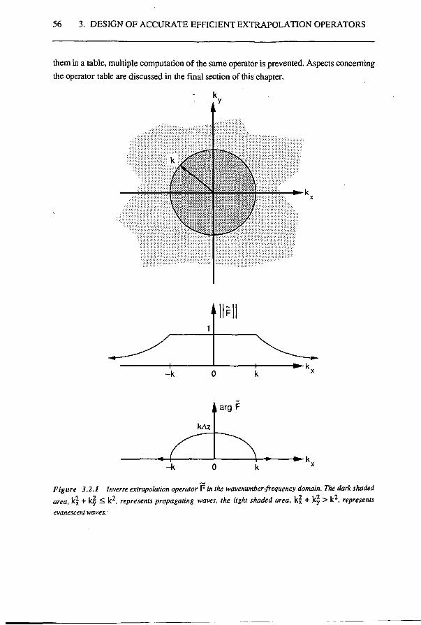
56 3. DESIGN OF ACCURATE EFFICIENT EXTRAPOLATION OPERATORS
them in a table, multiple computation of the same operator is prevented. Aspects concerning the operator table are discussed in the final section of this chapter.
♦ llF
iarg F
Figure 3.2.1 Inverse extrapolation operator F in the wavenumber-frequency domain. The dark shaded area, k2 + k2 < k2, represents propagating waves, the light shaded area, k 2 + k 2 > k2, represents evanescent waves.
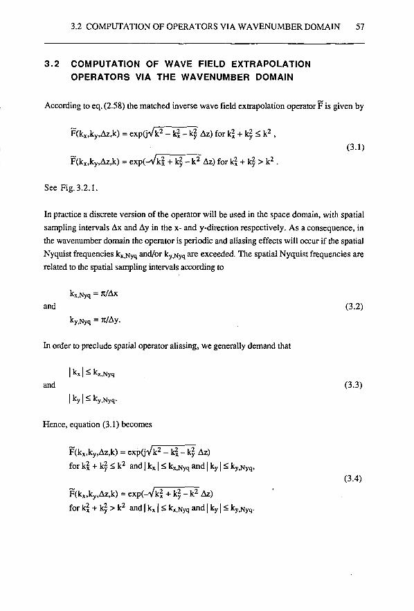
3.2 COMPUTATION OF OPERATORS VIA WAVENUMBER DOMAIN 57
3.2 COMPUTATION OF WAVE FIELD EXTRAPOLATION OPERATORS VIA THE WAVENUMBER DOMAIN
According to eq. (2.58) the matched inverse wave field extrapolation operator F is given by
F(kx,ky,Az,k) = exp(jVk2-k2-k2 Az) for k2 + tf <, k2 , (3.1)
F(kx,ky,Az,k) = exp(-Vk2 + k 2 - k 2 Az) for kjj + k2. > k2 .
See Fig. 3.2.1.
In practice a discrete version of the operator will be used in the space domain, with spatial sampling intervals Ax and Ay in the x- and y-direction respectively. As a consequence, in the wavenumber domain the operator is periodic and aliasing effects will occur if the spatial Nyquist frequencies kXfNyq and/or ky>Nyq are exceeded. The spatial Nyquist frequencies are related to the spatial sampling intervals according to
kx,Nyq = ItMx and (3.2)
ky,Nyq = I /Ay.
In order to preclude spatial operator aliasing, we generally demand that
| Kx | S KXiNyq
and (3.3) | ky I S ky_Nyq.
Hence, equation (3.1) becomes
F(kx,ky,Az,k) = expOVV-ki-k2 , Az) for k2 + k2 < k2 and | kx | <, kXjNyq and | ky | < kyiNyq,
(3.4) F(kx,ky,Az,k) = exp(-Vk? + k^-k 2 Az) for k£ + k > k2 and | kx | S kXtNyq and | ky | < kyiNyq.
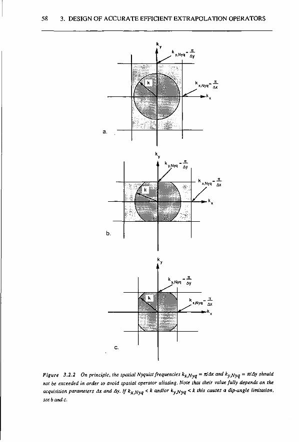
58 3. DESIGN OF ACCURATE EFFICIENT EXTRAPOLATION OPERATORS
x.Nyq AX
k = — y.Nyq Ay
_x,Nyq AX
\>1 ^
C.
Figure 3.2.2 On principle, the spatial Nyquist frequencies kx^yq = nlAx and ky^yq = nlAy should not be exceeded in order to avoid spatial operator aliasing. Note that their value fully depends on the acquisition parameters Ax and Ay. If kx^yq < k and/or ky^yq < k this causes a dip-angle limitation, see b and c.
3.2 COMPUTATION OF OPERATORS VIA WAVENUMBER DOMAIN 59
In Fig. 3.2.2 the situation in the wavenumber domain is shown for - kx,Nyq > k and ky,Nyq > k in a, - kXiNyq > k and kyjNyq < k in b and - kXiNyq < k and ky,Nyq < k in c.
The tilt angle of a propagating monochromatic plane wave (represented by one sample in the wavenumber-frequency domain) is given by
sin2a = ^ ± M f o r k 2 + k 2 < k 2 . k 2 y
(3.5)
See also Fig. 3.2.3. From this equation it becomes clear that the spatial band-limitation according to eq.(3.3) causes a dip-angle limitation in the extrapolated result if kx N y q<k and/or ky Nyq<k; see also Fig.3.2.2b and c. Preferably, the spatial Nyquist frequencies should therefore be larger than k. Unfortunately, as they are fully determined by the sampling intervals Ax and Ay (eq. (3.2)), they are fixed values after data acquisition.
k + k = k2sin2a
► k
Figure 3.2.3 Monochromatic plane waves propagating at a tilt angle a are represented by a circle in the kx,ky domain. The smaller the radius, the smaller the tilt angle.
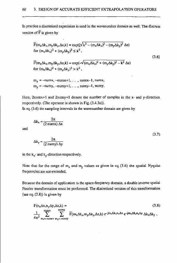
60 3. DESIGNOF ACCURATE EFFICIENT EXTRAPOLATION OPERATORS
In practice a discretized expression is used in the wavenumber domain as well. The discrete
version of F is given by
F(mxAkx,myAky,Az,k) = exp(jVk2 - (mxAkx)2 - (iriyAky)2 Az) for (mxAkx)2 + (myAky)2 < k2 ,
(3.6) F(mxAkx,myAky,Az,k) = exp(-V(n^Ak,)2 + (myAky)2 - k2 Az) for (mxAkx)2 + (myAky)2 > k2 ,
mx = -numx, -numx+1, . . ., numx-1, numx, my = -numy, -numy+1;. . ., numy-1, numy.
Here, 2numx+l and 2numy+l denote the number of samples in the x- and y-direction respectively. (The operator is shown in Fig. (3.4.3a)). In eq. (3.6) the sampling intervals in the wavenumber domain are given by
., 27t Akx=-(2 numx) Ax
and (3.7)
Ak - 2 * y (2 numy) Ay
in the kx- and ky-direction respectively.
Note that for the range of mx and my values as given in eq. (3.6) the spatial Nyquist frequencies are not exceeded.
Because the domain of application is the space-frequency domain, a double inverse spatial Fourier transformation must be performed. The discretized version of this transformation (see eq. (2.8)) is given by
F(nxAx,nyAy,Az,k) = (3.8) numx n u m y _
- J - £ £ F(mxAkx,myAky,Az,k) e-J1"»^"»^ e-Jn>yAkynyAy AkxAky , 4 1 m«=-numx my=-numy
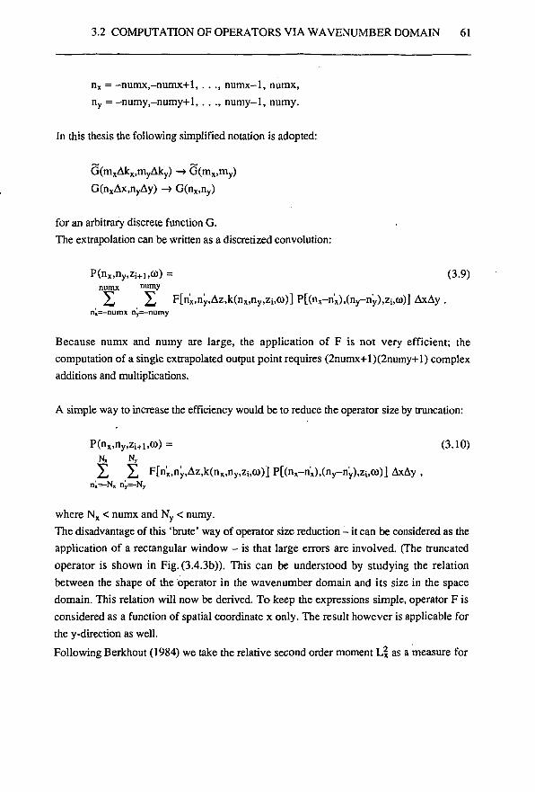
3.2 COMPUTATION OF OPERATORS VIA WAVENUMBER DOMAIN 61
nx = -numx,-numx+l,. . ., numx-1, numx, ny = -numy,-numy+l,.. ., numy-1, numy.
In this thesis the following simplified notation is adopted:
G(mxAkx,myAky) —»G(mx,my) G(nxAx,nyAy) -» G(nx,ny)
for an arbitrary discrete function G. The extrapolation can be written as a discretized convolution:
P(nx,ny,zi+1,co) = (3.9) numx n u m y X X F[nx,ny,Az,k(nx,ny,Zi,co)] PfCnx-n^.Cny-n^.Zi.co)] AxAy .
n»=-numx nj=-numy
Because numx and numy are large, the application of F is not very efficient; the computation of a single extrapolated output point requires (2numx+l)(2numy+l) complex additions and multiplications.
A simple way to increase the efficiency would be to reduce the operator size by truncation:
P(nx,ny>zi+1)co) = (3.10) N, Ny
X X F[n'x,ny,Az,k(nx,ny,Zi,co)] P[(nx-n'x),(ny-ny),Zi,a>)] AxAy ,
where Nx < numx and Ny < numy. The disadvantage of this 'brute' way of operator size reduction - it can be considered as the application of a rectangular window - is that large errors are involved. (The truncated operator is shown in Fig. (3.4.3b)). This can be understood by studying the relation between the shape of the operator in the wavenumber domain and its size in the space domain. This relation will now be derived. To keep the expressions simple, operator F is considered as a function of spatial coordinate x only. The result however is applicable for the y-direction as well. Following Berkhout (1984) we take the relative second order moment L | as a measure for
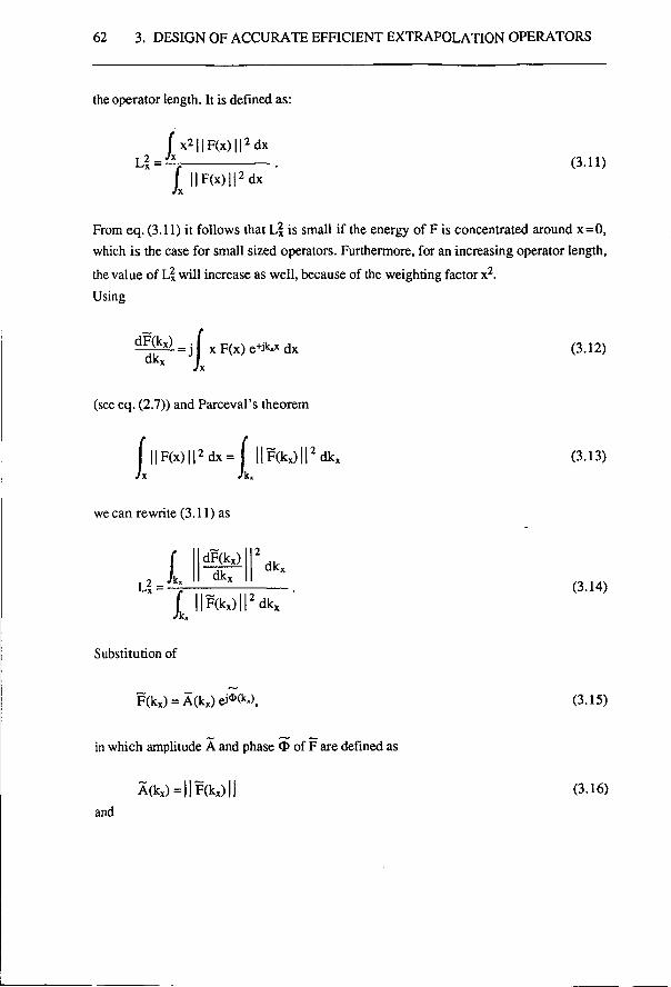
62 3. DESIGN OF ACCURATE EFFICIENT EXTRAPOLATION OPERATORS
the operator length. It is defined as:
£x2 | |F(x)| |2dx a=- Jj|F(x)||2dx
(3.11)
From eq. (3.11) it follows that L2 is small if the energy of F is concentrated around x=0, which is the case for small sized operators. Furthermore, for an increasing operator length, the value of L| will increase as well, because of the weighting factor x2. Using
dF(kx) dkx HI- F(x) e+Jk»x dx
(see eq. (2.7)) and Parceval's theorem
f | |F(x) | | 2dx = j iF(kx)irdkx
we can rewrite (3.11) as
L2 = 1. dF(kx) dkx
dkx
f llFOOH3 dk„
Substitution of
(3.12)
(3.13)
(3.14)
F(kx) = A(kx)eJ*(H (3.15)
in which amplitude A and phase O of F are defined as
A(kx)=||F(kx)| and
(3.16)
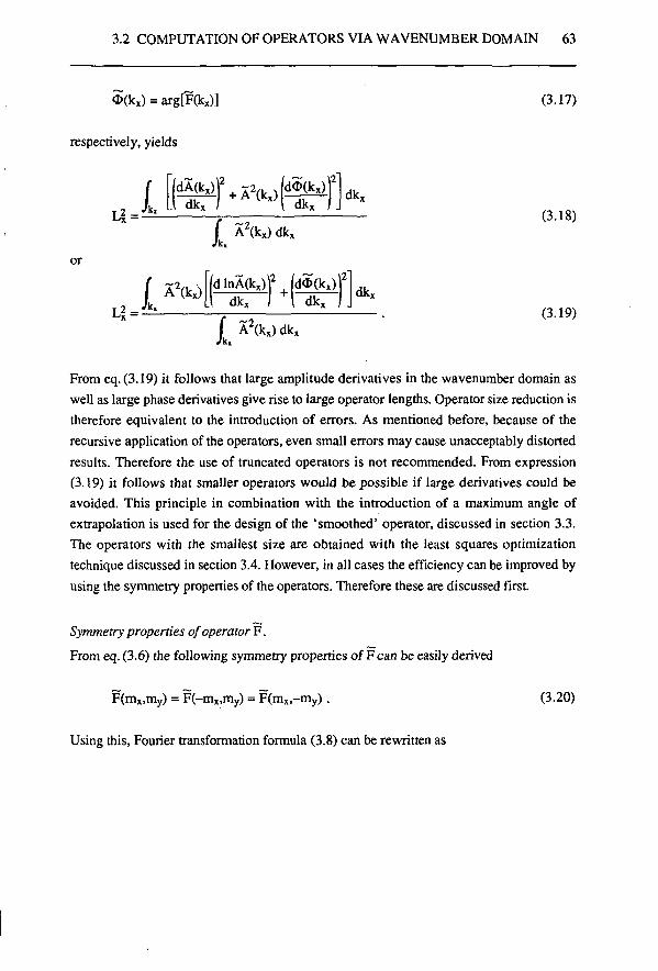
3.2 COMPUTATION OF OPERATORS VIA WAVENUMBER DOMAIN 63
<D(kx) = arg[F(kx)] (3.17)
respectively, yields
I (dA(kx)f + X2 ( k x ) (dO(k^ 2
dkx
U = - —r— — (3.18) f A2(k: x)dkx
or
i M^hi^l dkx
L£ = - ^ - . (3.19) A2(kx)dkx
From eq. (3.19) it follows that large amplitude derivatives in the wavenumber domain as well as large phase derivatives give rise to large operator lengths. Operator size reduction is therefore equivalent to the introduction of errors. As mentioned before, because of the recursive application of the operators, even small errors may cause unacceptably distorted results. Therefore the use of truncated operators is not recommended. From expression (3.19) it follows that smaller operators would be possible if large derivatives could be avoided. This principle in combination with the introduction of a maximum angle of extrapolation is used for the design of the 'smoothed' operator, discussed in section 3.3. The operators with the smallest size are obtained with the least squares optimization technique discussed in section 3.4. However, in all cases the efficiency can be improved by using the symmetry properties of the operators. Therefore these are discussed first.
Symmetry properties of operator F.
From eq. (3.6) the following symmetry properties of F can be easily derived
F(mx,my) = F(-mx,my) = F(mx,-my). (3.20)
Using this, Fourier transformation formula (3.8) can be rewritten as
64 3. DESIGN OF ACCURATE EFFICIENT EXTRAPOLATION OPERATORS
F(nx,ny>Az,k) = (3.21) numx numy __
—1— 2I1 X 4s(mx,my)F(mx>my,Az,k)cos(mxAkxnxAx)cos(myAkynyAy)AkxAky . 4n m,=o m,=o
Here s(mx,my) = 1 for mx >. 1 and my £ 1, s(mx,rriy) = 1/2 for (mx = 0 and my > 1) or (mx > 1 and my = 0) and (3.22) s(mx,my) = 1/4 for mx = 0 and my = 0.
From eq. (3.21) the following symmetry properties of operator F in the space domain can be derived
F(nx,ny) = F(-nx,ny) = F(nx,-ny). (3.23)
If these symmetry properties are used, the extrapolation, eq. (3.9), can be written as
numx n u m y P(nx,ny,zi+i,co) = £ X 4 s(n'x,ny) F[n'x,ny,Az,k(nX)ny,Zi,(ö)] (3.24)
{ P[(nx-nx),(ny-ny),Zi,co] +
P[(nx-nx),(ny+ny),Zi,co] +
P[(nx+nx),(ny-ny),zi,ü)] +
P[(nx+nx),(ny+ny),Zi,co] }AxAy.
The number of complex additions required to compute a single output point is approximately equal to the number of eq. (3.9). The number of complex multiplications however, has reduced by a factor of almost four to (numx+l)(numy+l). It is important to
notice that the use of the symmetry properties of F and F does not have any degrading effect on the accuracy of the extrapolation: eq. (3.24) is equivalent to eq. (3.9).
Maximum dip angle in wave field extrapolation. According to eq. (3.5) the angle a with respect to the vertical at which a monochromatic plane wave propagates, is given by
3.2 COMPUTATION OF OPERATORS VIA WAVENUMBER DOMAIN 65
k|+_k? k2 sin 2cc = x_n
y for k\ + k2 < k2 (3.25)
or k* + — ^ — = l f o r a * 0 a n d k 2 + k 2 < k 2 .
k2sin2a k2sin2a (3.26)
Note that all waves with the same angle can be found on a circle, see Fig. 3.2.3. Waves propagating at smaller angles are represented in the area within this circle, and waves propagating at larger angles as well as evanescent waves correspond to the outside area.
As mentioned, the introduction of a maximum angle of extrapolation enables us to design more efficient wave field extrapolation operators. The maximum extrapolation angle o ^ ^ (0°<amax<90°) is defined as
k2 +k2
sin2ccmax(kx,ky) = x y (3.27 a) kz
where kx and ky are on the ellipse
k?. ■ = 1. (3.27b)
k2. . Ü k Sin Ctx,max k Sin CCy>max
Here ax max (0°<ax max<90°) is the maximum angle of extrapolation in the x-direction and ocy max (00<OCymax<900) is the maximum angle of extrapolation in the y-direction. According to eq. (3.27b) the waves with extrapolation angle ocmax can be found on an ellipse in the wavenumber-frequency domain. Hence, this maximum angle is not a constant: it is a function of kx and ky, see Fig. 3.2.4. The reason for defining different maximum angles of extrapolation for the x- and y-direction is that the spatial sampling intervals Ax and Ay and so the spatial Nyquist frequencies are usually different as well. By defining operators that approximate F very well in the area within the ellipse as defined in eq. (3.27), but that are allowed to deviate from F in the area outside this ellipse, an increased efficiency can be reached. This is the topic of the next sections. However, first an error criterion is derived. This will be used to determine the maximum amplitude and phase errors of an approximated operator that are allowed such that the extrapolation results are still acceptable and stable.
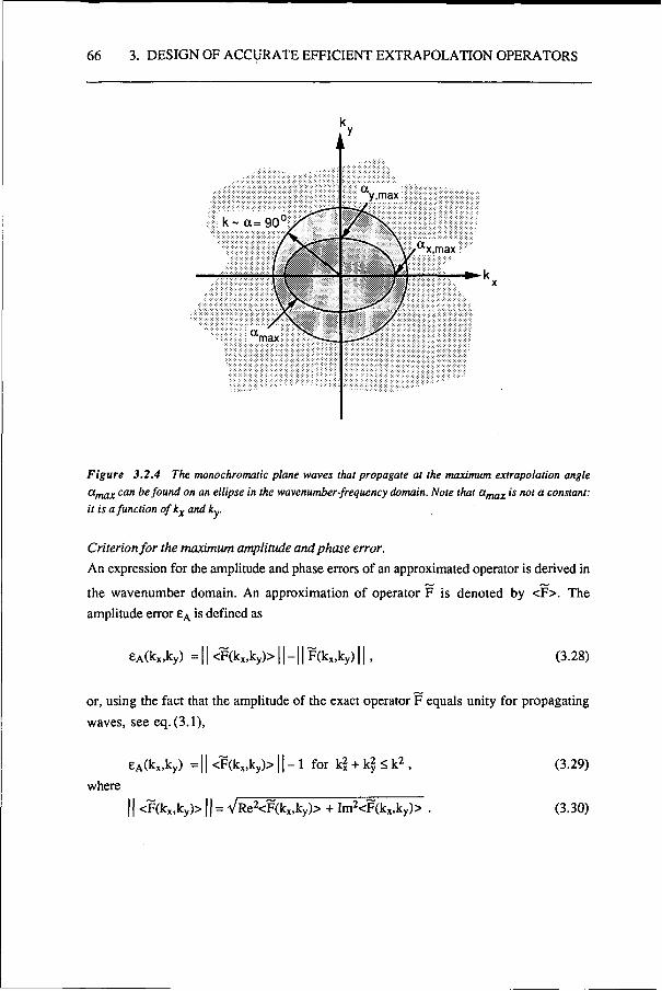
66 3. DESIGN OF ACCURATE EFFICIENT EXTRAPOLATION OPERATORS
Figure 3.2.4 The monochromatic plane waves that propagate at the maximum extrapolation angle amax can be found on an ellipse in the wavenumber-frequency domain. Note that ccmax is not a constant: it is a function of kx and ky.
Criterion for the maximum amplitude and phase error. An expression for the amplitude and phase errors of an approximated operator is derived in the wavenumber domain. An approximation of operator F is denoted by <F>. The amplitude error eA is defined as
eA(kx,ky) = 11 <F(kX)ky)> 11-| | F(kx,ky) 11, (3.28)
or, using the fact that the amplitude of the exact operator F equals unity for propagating waves, see eq. (3.1),
eA(kx,ky) = 11 <F(kx,ky)> 11 - 1 for k2 + k2 <> k2 , where
11 <F(kx,ky)> 11 = VRe2<F(kx,ky)> + Im2<F(kx,ky)> .
(3.29)
(3.30)
3.2 COMPUTATION OF OPERATORS VIA WAVENUMBER DOMAIN 67
The phase error e<& is defined as
e<t,(kx,ky) = arg <F(kx,ky)> - arg F(kx,ky).
From eq. (3.1) it follows that
F(kx,ky) = V k 2 - k l - t ó Az for k2 + k2 < k2 . arg
Substitution in eq.(3.31) yields
e<t,(kx.ky) = arg <F(kx>ky)> - V k 2 - k 2 - k 2 Az for k2 + k2. < k2 , where
arg <F(kx,ky)> = arctan Im <F(kx,ky)> Re <F(kx,ky)>
(3.31)
(3.32)
(3.33)
(3.34)
If the approximated operator <F> is used, the total amplitude error after N extrapolation steps is
[ l+eA(k x ,k y)]N-[ l ]N . (3.35)
If the amplitude error is small: EA(kx,ky) « 1, the total amplitude error after N extrapolation steps can be expressed as
or
[l+NeA(kx ,ky)]-[l]
NeA(kx,ky). (3.36)
Because the phase errors simply add up each extrapolation step, the total phase error after N extrapolation steps is
Ne4)(kx,ky) (3.37)
Hence, the total error after N extrapolation steps equals the sum of the errors made in each extrapolation step. According to equations (3.36) and (3.37) this holds for the amplitude
68 3. DESIGN OF ACCURATE EFFICIENT EXTRAPOLATION OPERATORS
error as well as for the phase error. Note that these expressions were obtained by assuming that the errors are equal at each extrapolation step. This is a 'worst case' assumption: in practice the errors vary which means that the accumulation of errors may be less severe.
In case of a maximum angle of extrapolation cc,^, the errors are only defined for angles smaller than amax (the area in the wavenumber domain within the ellipse as defined by eq.(3.27)). If one accepts a total maximum amplitude error EA in the extrapolated result at the maximum extrapolation depth NAz, this yields
| NeA(kx,ky) | < EA for — — ^ + — — ^ ^ 1 (3.37) kzSinzCCx,max k^Sin^OCy.max
or
|eA(kX )ky) | ,fA f o r ^ _ + s ^ - , i. (3.38) K sin «x.max K *'" uy,max
For the total maximum phase error at the maximum extrapolation depth the value E^ is accepted. This leads to
| e<t>(kx,ky) | £ 5 * for —f + -—f £ 1. (3.39) 1N kzsin2ax.max k /sin /av.max
For the part of the waves that propagate at angles larger than a^m and the evanescent field there are no special requirements as far as the phase errors are concerned. However, instability should always be precluded and therefore we demand that
eA(kx,kv) < | f for all kx and k„ . (3.40) ' N
Furthermore, optionally, the amplitude of the part of the wave field for cc£amax and the evanescent field can be suppressed. We introduce the window error function Eu according to
eu(kx,ky) = 11 <F(kx,ky)> 11 - U(kx,ky), (3.41)
where U is a user-specified amplitude window, e.g., a cosine window. It satisfies
3.3 SMOOTHED EXTRAPOLATION OPERATOR 69
0 < Ü(kx,ky) < 1 . (3.42)
Our requirement for suppression is
e u ( k x > k y ) < E A f o r ^ + - — ^ > 1. , (3.43) N k- sin ax.max k':sinzay,max
Note that the stability requirement, eq. (3.40) is automatically included in eq. (3.38) and eq.(3.43). Berkhout (1985) proposes a value of rc/10 for the maximum amplitude error EA as well as for the maximum phase error E^. In case of 50 extrapolation steps the thresholds in eq. (3.39) and (3.40) both amount to 0.006.
3.3 SMOOTHED EXTRAPOLATION OPERATOR
In the previous section we have already mentioned that operator F has large derivatives with respect to kx and ky. According to the relation between the shape of an operator F in the wavenumber domain and the size of its equivalent F in the space domain, eq.(3.19),
large derivatives that occur in F correspond to a large-sized operator F. This is unattractive for a practical application. If smaller operators in the space domain are desired, because they can be applied more efficiently, their equivalent in the wavenumber domain should not have large derivatives. In this chapter two solutions are discussed. We start with the 'smoothed' operator that is designed according to the above mentioned requirement. In the next section we discuss the 'optimized' operator. The 'smoothed' operator is defined as:
Fs(kx,ky,Az,k) = exp(jVk2-kx-kyAz) kx k* for ——-^ + ——-^ < 1 and | kx | £ kx,Nyq and | ky | < ky,Nyq ,
k^sin^ax.max k^sm^ay.max (3.44)
Fs(kx,ky,Az,k) = As(kx,ky,k) exp[jOs(kx,ky,Az,k)]
70 3. DESIGN OF ACCURATE EFFICIENT EXTRAPOLATION OPERATORS
k2 k2
for ——-^ + ——-Z > 1 and|kx |<kX i N y qand|ky |£ky ,N y q . k^sin^ax.max kzsinzay,max
In this equation As, the optional user-specified amplitude window, and phase <I>S are smooth functions that are defined such that Fs as well as its first derivatives with respect to kx and ky are continuous at
kl . Ü k2sin2ax,max k2sin2ay,max
= 1 at | kx | = kXiNyq and at | ky | = kyiNyq .
The index s refers to the smooth character of the operator which is therefore called 'smoothed operator'. For waves that propagate at angles smaller than o^^ operator Fs is exact, (compare with eq. (3.1)). For waves that propagate at larger angles and evanescent waves, the phase of Fs
is incorrect. However, optionally this part of the wave field can be suppressed with the amplitude window As.
In practice we use the following simplified version of eq. (3.44)
Fs(kx,ky,Az,k) = exp(jVk2 - kr2 Az)
for kr £ ksinoCmax and | kx | S kXiNyq and | ky | < kyiNyq ,
Fs(kx,ky,Az,k) = As(kx,ky,k) exp[j<I)s(kx,ky,Az,k)] for kr > ksinoCmax and | kx | < kXiNyq and | ky | < ky,Nyq .
(3.45)
Here kr = Vk2 + k2 .
The amplitude window As in eq. (3.45) is given by a cosine function:
As(kx,ky,k) = ai + (l-aO 1 / k ^ c s i n o , ^ ! + t 2 \ kr.Nyq-ksinCtmax/ 2
for kr > ksinocmax and kr < kr>Nyq ,
As(kx,ky,k) = a!
(3.46)
3.3 SMOOTHED EXTRAPOLATION OPERATOR 71
for kr > krj>fyq and | kx | < kx>Nyq and | ky | < ky,Nyq.
Here k, Nyq is defined as
kr,Nyq = min(kx,Nyq> ky,Nyq> (3.47)
and coefficient aj must satisfy: 0 £ aj < 1.
In eq. (3.45) phase function 4>s is given by
0>s(kx>ky,Az,k) = a(Az,k)k? + b(Az,k)k? + c(Az,k)kr + d(Az,k) for kr > ksinctmax and kr < kriNyq,
(3.48) <Ds(kx,ky,Az,k) = 0 for kr > krtNyq and kx < kXjNyq and ky < kyiNyq.
The value of a , ^ is chosen such that it always satisfies
ksinamax < 0.85 kr,Nyq . (3.49)
The spline coefficients a, b, c and d in eq. (3.48) are defined by the following four boundary conditions: G>s and its first derivative with respect to kr are continuous at kr=ksinamax and zero at 1 ^ = ^ ^ .
Note that eq. (3.45) is somewhat less general than eq. (3.44) because we introduced circular symmetry by defining Fs to be a function of kj instead of kx and ky. This implies that sinaxmax = sinOL,imax = sinamax. The advantage of these assumptions is that relatively simple expressions for As and Os can be formulated. The smooth operator is shown in Fig. 3.3.1, (see also Fig.(3.4.3c)).
The discrete expression for Fs can be found from eqs.(3.45) to (3.48) by substituting mxAkx for kx and myAky for ky, where mx ranges from -numx to numx and my ranges from -numy to numy.
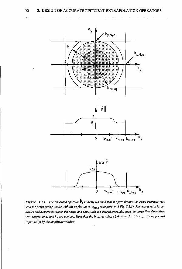
72 3. DESIGN OF ACCURATE EFFICIENT EXTRAPOLATION OPERATORS
x.Nyq
M F
-I h 0 'amax' *V,Nyq k x N y q x
^r.Nyq ^x,Nyq
Figure 3.3.1 The smoothed operator F s is designed such that it approximates the exact operator very well for propagating waves with tilt angles up to c^a* (compare with Fig. 3.2.1). For waves with larger angles and evanescent waves the phase and amplitude are shaped smoothly, such that large first derivatives with respect to kx and ky are avoided. Note that the incorrect phase behaviour for a > a^^ is suppressed (optionally) by the amplitude window.
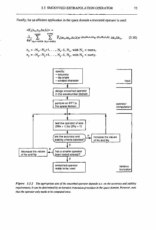
3.3 SMOOTHED EXTRAPOLATION OPERATOR 73
Finally, for an efficient application in the space domain a truncated operator is used:
<Fs(nx,ny,Az,k)> = numx numy ____
- ^ I X Fs(mx>my,Az,k)e-Jm»Ak«n'Axe-JmyAk»nyAyAkxAky, (3.50) 4ft m»=-numx m,=-numy
nx = -N x , -N x+1 N x - 1 , Nx , with Nx < numx, ny = -N y , -N y +1 , . . ., N y - 1 , Ny , with N y < numy.
specify. - accuracy -dip-angle - window character input
design smoothed operator in the wavenumber domain
perform an FFT to the space domain
test the operator of size (2Nx+1)by(2Ny + 1)
e are the accuracy and ^ n
stability criteria satisfied?
decrease the values of Nx and Ny R has a smaller operatoi
been tested already rj smoothed operator ready to be used
operator computation
increase the values of Nx and Ny
iterative truncation
Figure 3.3.2 The appropriate size of the smoothed operator depends a.o. on the accuracy and stability requirements, ft can be determined by an iterative truncation procedure in the space domain. However, note that the operator only needs to be computed once.
74 3. DESIGN OF ACCURATE EFFICIENT EXTRAPOLATION OPERATORS
Because of the smooth shape of operator Fs in the wavenumber domain, we expect that the negative effects of the use of a truncated operator <FS> in the space frequency domain remain limited, see also eq.(3.19). (This in contrast with the use of a truncated operator according to eq. (3.10)). Nevertheless, errors are also introduced. For the high-angle part of the wave field, with a xXmj,, and the evanescent part this is no problem as long as the requirements concerning stability (eq. (3.40)) or suppression (eq. (3.43)) are satisfied. For the part of the wave field with aScc,,^ it might be necessary to increase the operator size, i.e., to increase the values of Nx and Ny. On the other hand, if the accuracy turns out to be better than the pre-specified value, the operator size may be reduced. The procedure is visualized in Fig. 3.3.2. Note that the operator is computed once. Thereafter, only the number of operator points is varied. This causes the computation of the operators to be very fast: a table containing the operators (see section 3.5) can be easily generated at the beginning of the application program. We have already mentioned a second operator type: the 'optimized' operator. It turns out that 'optimized' operators are even more efficient than 'smoothed' operators. Unfortunately, the computation of the 'optimized' operators is in itself such a time consuming process that it is not feasible to generate them at the beginning of the program. Instead, prior to application one should have available operator sets for the most common acquisition parameters. The 'optimized' extrapolation operator will be discussed next.
3.4 OPTIMIZED EXTRAPOLATION OPERATOR
Although the extrapolation results with the smoothed operator are fully satisfactory, the efficiency in not yet optimum. Only by computing the operator coefficients such that the errors are minimized, one can be sure that the smallest possible operator has been found, given a pre-defined accuracy. The operator optimization method, introduced by Holberg (1988) for the 2D case, has some properties that make it very suitable for our purpose: - the operator size (the number of operator points) and the maximum dip-angle are user-
specified input parameters, - optionally the operator can be designed such that it acts as a high dip-angle or
evanescent field suppression filter, and - the most accurate operator possible under the above mentioned conditions is found.
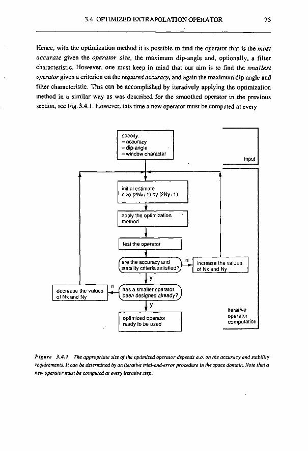
3.4 OPTIMIZED EXTRAPOLATION OPERATOR 75
Hence, with the optimization method it is possible to find the operator that is the most accurate given the operator size, the maximum dip-angle and, optionally, a filter characteristic. However, one must keep in mind that our aim is to find the smallest operator given a criterion on the required accuracy, and again the maximum dip-angle and filter characteristic. This can be accomplished by iteratively applying the optimization method in a similar way as was described for the smoothed operator in the previous section, see Fig. 3.4.1. However, this time a new operator must be computed at every
specify: - accuracy - dip-angle - window character
input
initial estimate size(2Nx+1)by(2Ny+1)
apply the optimization method
test the operator
d are the accuracy and stability criteria satisfied?,
decrease the values of Nx and Ny vu*
increase the values of Nx and Ny
has a smaller operator been designed already? D optimized operator ready to be used
iterative operator computation
Figure 3.4.1 The appropriate size of the optimized operator depends a.o. on the accuracy and stability requirements. It can be determined by an iterative trial-and-error procedure in the space domain. Note that a new operator must be computed at every iterative step.
76 3. DESIGN OF ACCURATE EFFICIENT EXTRAPOLATION OPERATORS
iterative step. This makes the computation of a set of operators quite time consuming. Therefore it is not recommended to compute a table of optimized operators at the beginning of each application program (like we suggested for the smoothed operator). Instead a library of tables containing optimized operators for the most common acquisition parameters should be available. A description of the optimization method, which we extended to the 3D case, is given next.
The basic principle of the operator optimization is to minimize in a least-squares sense the phase and amplitude errors as defined in section 3.2. The option to make the operator also act as a high dip-angle and evanescent field suppressor can be realized by including the amplitude window function in a so-called constraint function. The procedure is as follows. First the requirements concerning the accuracy of the operator, its dip-angle performance and the window characteristics are formulated. An arbitrary initial estimate of the optimized operator (e.g., a smoothed operator) is Fourier transformed from the space domain to the wavenumber domain according to
N, Ny
< F 0 ( m x , m y ) > = ] £ £ < F 0 ( n x , n y ) > ejmxAk,n,AxejmyAkynyAy A x A y ( ( 3 . 5 1 )
n„=-Nx n^-Ny
mx = -numx, -numx+1,. . ., numx-1, numx, my = -numy, -numy+1,. . ., numy-1, numy.
The index o refers to 'optimized' operator. Note that the size of the operator, determined by Nx and N , is still arbitrary. Next, the amplitude and phase errors in the wavenumber domain are computed according to (3.29) and (3.33). Here we give the discrete versions. The amplitude error is:
eA(mx,my) = VRe2<F0(mx,my)> + Im2<F0(mx,my)> - 1 for (3.52)
(mxAkx)2 t (myAky)2
k2sin2(ocx,max) k2sin2(ay,max) with
mx = -numx, -numx+1, . . ., numx-1, numx, my = -numy, -numy+1,. . ., numy-1, numy.
3.4 OPTIMIZED EXTRAPOLATION OPERATOR 77
The phase error is evaluated according to
Im<F0(mx>my)> ed>(mx,my) = arctan - Vk2 - (mxAkx)2 - (myAky)2 Az
Re<F0(mx,my)> for (3.53)
(mxAkx)2 ^ (rriyAky)2 ■+ -~y—y < i ,
k2sin2(ax,max) k2sin2(ay,max) with
mx = -numx, -numx+1, . . ., numx—1, numx, my = -numy, -niimy+1, . . ., nuiny-1, numy.
Furthermore, the window error function tu (eq. 3.41) is evaluated:
Eu(mx,niy) = VRe2<F()(mx,iny)> + Im2<F0(mx,my)> — U(mx,niy) for (3.54)
(mxAkx)2 t (myAky)2
-> 1 k2sin2(ax,max) k2sin2(ay,max)
with mx = -numx, -numx+1, . . ., numx-1, numx, my = -numy, -numy+1, . . ., numy-1, numy.
The optimization problem can be summarized as follows. Find the operator coefficients <F0(nx,ny)> such that the following requirements are met: 1. in the dark shaded area as depicted in Fig. 3.4.2 the phase and amplitude errors are as
small as possible, 2. in the light shaded area of Fig. 3.4.2 the operator satisfies the requirements concerning
suppression (eu(kx,ky)SEA/N) or stability (eA(kx,ky)<EA/N).
In the implementation of the optimization method two functions are important: the objective function O, which handles requirement 1 and the constraint function C, which takes care of requirement 2. These functions are now discussed.
The error function that is minimized, requirement 1, is called the objective function and is given by
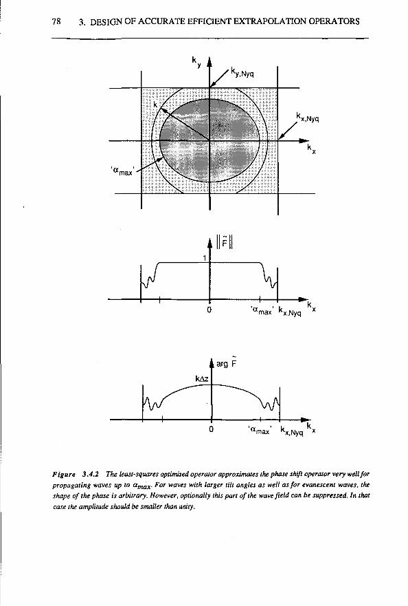
78 3. DESIGN OF ACCURATE EFFICIENT EXTRAPOLATION OPERATORS
amax kx,Nyq
max x.Nyq
Figure 3.4.2 The least-squares optimized operator approximates the phase shift operator very well for propagating waves up to amax. For waves with larger tilt angles as well as for evanescent waves, the shape of the phase is arbitrary. However, optionally this part of the wave field can be suppressed. In that case the amplitude should be smaller than unity.
3.4 OPTIMIZED EXTRAPOLATION OPERATOR 79
numx numy O [<F0(nx,ny)>] = £ X [ 4(mx ,my) + ^e£(mx,my) ] , (3.55)
m,=-numx my=-numy with
nx = - N x , - N x + l , . . . , N x - l , N x , ny = -Ny, -Ny+1, . . ., Ny-l,Ny.
In this equation, the summation is carried out over all kjjcy samples that are within the area as defined by
^ A k ^ + ^ ^ _ < i a n d | k x | < k x N y q a n d | k y | S k y N y q ) (3.56 )
kzsinz(ax,max) k^sin^ocy .max)
see the dark shaded area in Fig. 3.4.2. The optional weighting factor \i can be used to control the emphasis put on the amplitude errors relative to the phase errors. In practice we use \L = 1.
Requirement 2, concerning stability or suppression of the larger wavenumbers, is formulated in a constraint function. Although the actual requirement is simply eu(kxJcy)SEA/N, for minimization software the following function need be implemented:
numx numy / \2 C [<F0(nx,ny)>] = X X max[(eu(mx,my)-^),0] = 0 , (3.57)
mx=-mimx m,=-numy V / with
nx = -Nx, -Nx+1, . . ., NX-1,NX, ny = "Ny, "Ny + 1, . . ., Ny-l,Ny.
Here, the summation is carried out over the kx,ky samples that are within the area as defined by
, ( m , x M x ) 2 + -r^-m,yAky)2 > 1 and | kx | £ kx,Nyq and | ky | < ky,Nyq , (3.58) kzsin/(ax>max) kzsinz(ccy,max)
see the light shaded area in Fig. 3.4.2.
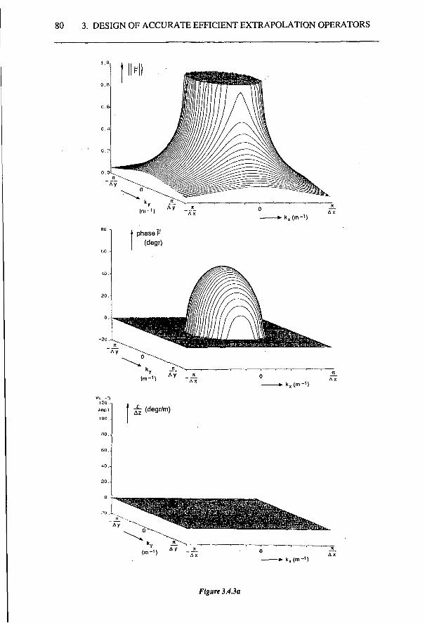
80 3. DESIGN OF ACCURATE EFFICIENT EXTRAPOLATION OPERATORS
(m-M kx(m-M
Figure 3.4 Ja
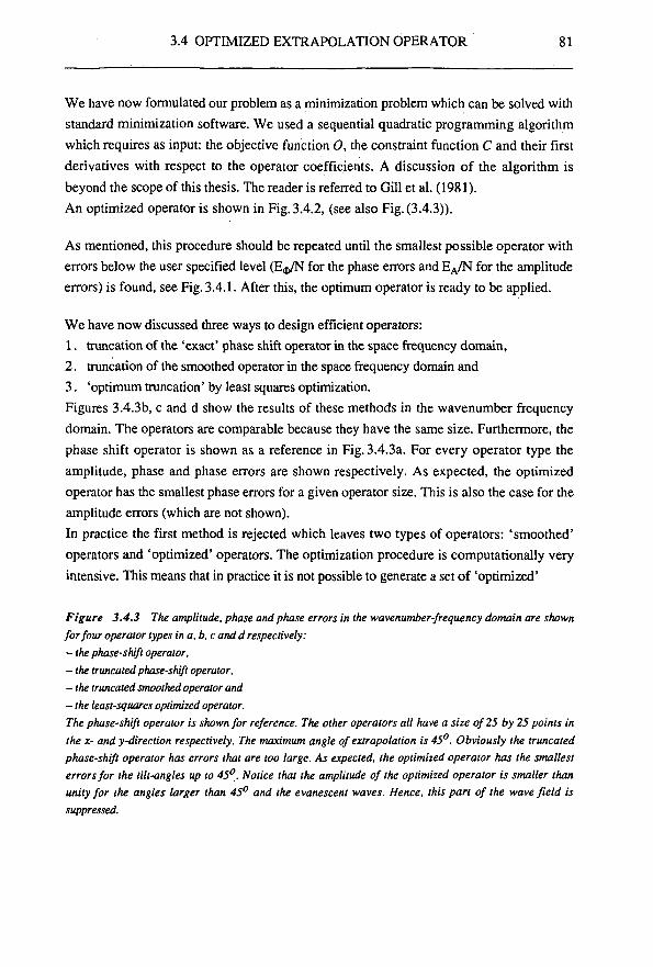
3.4 OPTIMIZED EXTRAPOLATION OPERATOR 81
We have now formulated our problem as a minimization problem which can be solved with standard minimization software. We used a sequential quadratic programming algorithm which requires as input: the objective function 0, the constraint function C and their first derivatives with respect to the operator coefficients. A discussion of the algorithm is beyond the scope of this thesis. The reader is referred to Gill et al. (1981). An optimized operator is shown in Fig. 3.4.2, (see also Fig. (3.4.3)).
As mentioned, this procedure should be repeated until the smallest possible operator with errors below the user specified level (E^/N for the phase errors and EA/N for the amplitude errors) is found, see Fig. 3.4.1. After this, the optimum operator is ready to be applied.
We have now discussed three ways to design efficient operators: 1. truncation of the 'exact' phase shift operator in the space frequency domain, 2. truncation of the smoothed operator in the space frequency domain and 3. 'optimum truncation' by least squares optimization. Figures 3.4.3b, c and d show the results of these methods in the wavenumber frequency domain. The operators are comparable because they have the same size. Furthermore, the phase shift operator is shown as a reference in Fig. 3.4.3a. For every operator type the amplitude, phase and phase errors are shown respectively. As expected, the optimized operator has the smallest phase errors for a given operator size. This is also the case for the amplitude errors (which are not shown). In practice the first method is rejected which leaves two types of operators: 'smoothed' operators and 'optimized' operators. The optimization procedure is computationally very intensive. This means that in practice it is not possible to generate a set of 'optimized'
Figure 3.4.3 The amplitude, phase and phase errors in the wavenumber-frequency domain are shown for four operator types in a,b,c and d respectively: - the phase-shift operator, - the truncated phase-shift operator, - the truncated smoothed operator and - the least-squares optimized operator. The phase-shift operator is shown for reference. The other operators all have a size of 25 by 25 points in the x- and y-direction respectively. The maximum angle of extrapolation is 45°. Obviously the truncated phase-shift operator has errors that are too large. As expected, the optimized operator has the smallest errors for the tilt-angles up to 45°. Notice that the amplitude of the optimized operator is smaller than unity for the angles larger than 45° and the evanescent waves. Hence, this part of the wave field is suppressed.
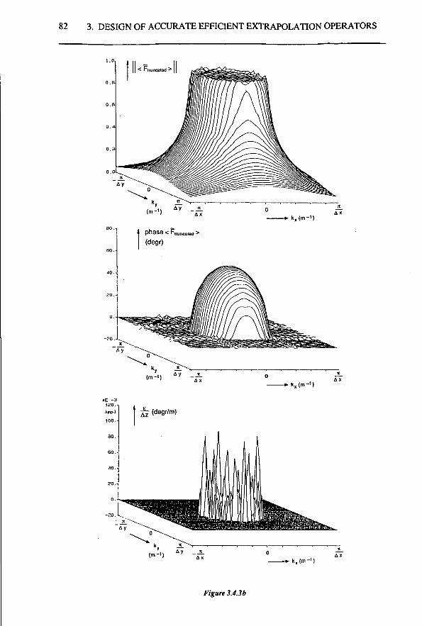
82 3. DESIGN OF ACCURATE EFFICIENT EXTRAPOLATION OPERATORS
k„(m-')
Figure 3.4.3b
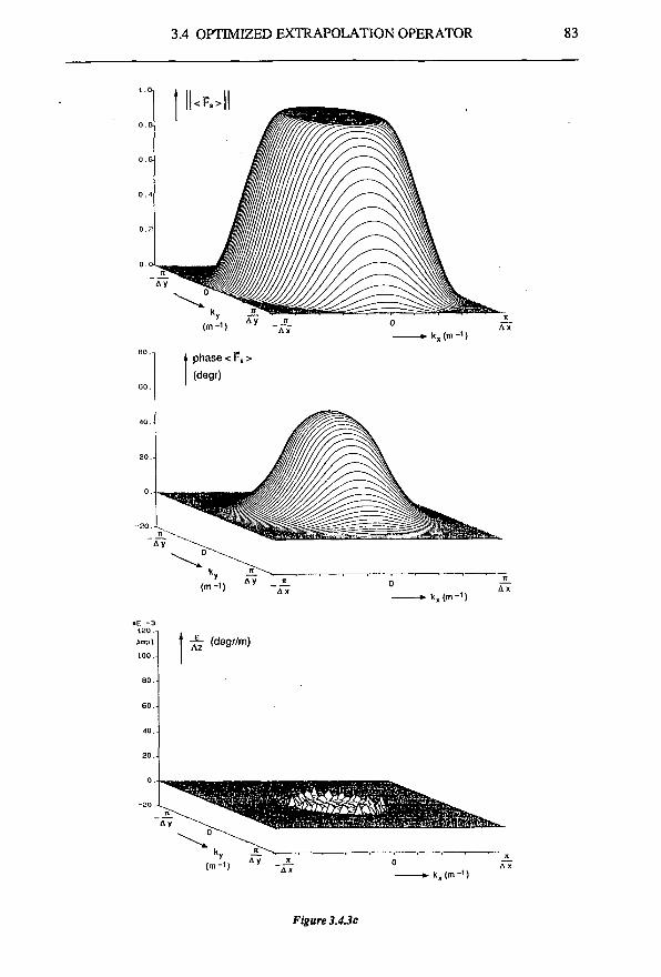
3.4 OPTIMIZED EXTRAPOLATION OPERATOR 83
(m-M - . » A> -kx(m-n
«E - 3 120 . Ampl 100. -
Az (degr/m)
PMI1 ("--» Ay -i7 -»• kx(m-M
Figure 3.4.3c
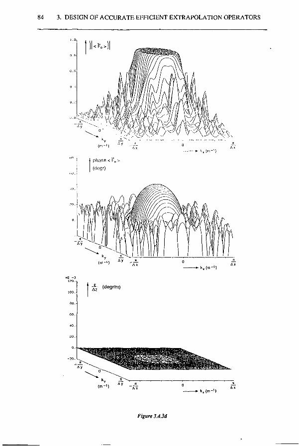
84 3. DESIGN OF ACCURATE EFFICIENT EXTRAPOLATION OPERATORS
*• k„ (m- ' )
«E - 3 120.- ,
' ^ (degr/m)
(m-i) k , ( m - ' )
Figure 3.4.3d
3.5 OPERATOR TABLE 85
operators during application. We suggest that one should have available a number of operator tables (see the next section) for the most common acquisition parameters. This enables the user to take advantage of the superior efficiency of the 'optimized' operators in regular cases. In other cases (no 'optimized' operators available, specific acquisition parameters) 'smoothed' operators can be used. The results are equivalent to those obtained with 'optimized' operators, but the extrapolation is less efficient.
Because the number of variables is large: Ax, Ay, Az, ocxmax, ocymax, k, U, EA, Ey and E,j„ it is difficult to give values for the size of the operator, (2Nx+l)(2Ny+l). As a rule of thumb we use:
Nx > 1/20lX)inax (expressed in degrees) and Ny £ 1/20tyimax (expressed in degrees)
for the 'smoothed' operator, and Nx> 1/4axmax (expressed in degrees) and Ny > 1/4aymax (expressed in degrees)
for the 'optimized' operator. For an extensive study on this subject, we refer to Debeye (1988).
3.5 OPERATOR TABLE
The methods of operator generation as described in the previous sections are rather computationally intensive, especially the operator optimization method. Computation of the operators during the extrapolation would slow down the speed of the algorithm. Furthermore, a specific operator is likely to be required more than once. This can be explained as follows. A unique operator is necessary for every unique value of the wavenumber, k=co/c(x,y,z). However, a certain value for k is likely to occur many times within one extrapolation process. This is because a certain frequency component will be treated many times (because of the recursive character of the extrapolation) and a certain velocity will occur more than once (in practice, a macro model contains large constant velocity areas). Another possibility is that both the value of the frequency and that of the velocity change such that their ratio k remains unaltered. Also in this case the same operator can be used. For these reasons, the operators are computed separately in advance and stored in a table. This way the same operators can be used efficiently for a range of
86 3. DESIGN OF ACCURATE EFFICIENT EXTRAPOLATION OPERATORS
extrapolation steps as well as for a range of frequencies. Finally, we remark that it is possible to use a set of operators in a future processing job. During the extrapolation, the local value of the wavenumber k is determined after which the appropriate operator is selected from the table and applied to the data. This procedure however, might lead to a very large operator table. The reason is that the maximum number of different k-values is large: it equals the number of subsurface grid points times the number of frequency components (this maximum might occur in the case that the velocity changes from point to point in the subsurface, e.g. if the macro model has velocity gradients). We therefore decided not to keep an operator in the table for every k-value that occurs, but to define a wavenumber sampling interval Ak and to store operators in the table for the following regular range of k-values only:
kmin. kmin + ^ ^ • • • ' kmax - Ak, k , ^ , (3.59)
in which kmin=comin/cmax and kmax = comax/cmin. Note that the number of operators in the table is inversely proportional to Ak. The advantage of such a table is its limited size. The disadvantage is that an actually required operator is not likely to be present. There are several ways to solve this problem. The easiest way to 'compute' an operator for a k-value that is not present in the table is to select the operator with a k-value nearest to the required one. The disadvantage of the method is that the phase and amplitude errors due to the rounding off may accumulate systematically each extrapolation step which causes dispersion effects. The more homogeneous a macro model is, the more serious the dispersion effects are. Therefore the interval Ak should be very small. As a consequence the number of operators might become so large that storage of the operator table in core memory would be impossible. Hence, the rounding method is not recommended. Systematic accumulation of errors does not occur when 'statistical rounding' is used. The method can be explained most easily with an example. Suppose that in the table operators are present for k= 1 and for k = 2 and suppose that an operator is required for k= 1.4. In this case either the operator for k= 1 is selected with a probability of 0.6 or the operator for k=2 is selected with a probability of 0.4. It is clear that here also rounding errors occur; however, they do not accumulate. Experiments indicate that 'statistical rounding' allows the table size to be reduced by a factor of seven compared with 'rounding'. Notice that 'statistical rounding' is almost as simple as 'rounding': it only requires a random generator. Nevertheless a much smaller operator table is sufficient.
3.5 OPERATOR TABLE 87
If a better accuracy is demanded, or if even more memory must be saved, it is worthwhile to compute a required operator by means of interpolation. We found that in general linear interpolation of real and imaginary parts gives good results if Ak is in the order of AoV2cmax. This interval is about thirty times as large as the interval required by 'rounding'. Unlike 'rounding' and 'statistical rounding', 'linear operator interpolation' increases the computational cost. However, in practical situations, where the macro model contains large homogeneous areas, this extra effort can be neglected if it is compared with the actual extrapolation. In our extrapolation schemes we therefore use 'linear operator interpolation'.

89
CHAPTER 4
APPLICATION OF RECURSIVE KIRCHHOFF EXTRAPOLATION OPERATORS IN MIGRATION
4.1 INTRODUCTION
The recursive Kirchhoff extrapolation operators as discussed in the previous chapter, the smooth operator and the optimum operator, can be used for a wide variety of applications. E.g., they can be applied in all prestack and poststack migration methods that are based on the principle of recursive wave field extrapolation and imaging. Another possibility is the use of the operators for redatuming. A redatuming algorithm can be obtained from a migration algorithm simply by omitting the imaging step. However, a redatuming scheme based on recursive extrapolation is not preferred: one is not interested in the intermediate extrapolation results (which are required in migration for the imaging step). Because of the computational cost of recursive extrapolation, a non-recursive technique is recommended for redatuming (Peels, 1988, Kinneging, 1989), see also section 1.5. We also mention the application of the recursive Kirchhoff extrapolation operators in the modeling of seismic data. In the appendix the modeling of 3D zero-offset data is discussed. In this chapter the emphasis is on seismic migration. Three techniques are considered: prestack migration, common-offset migration and zero-offset migration. The best results are obtained with prestack migration. However, full 3D prestack migration is not yet feasible on present computers. Although we will discuss the 3D prestack case, we implemented prestack migration for the 2D case. In order to make 3D migration feasible the amount of data that is involved should be reduced. E.g., instead of incorporating all offsets of each shot in the migration, one could use one specific offset per shot only. This type of migration is called common-offset migration. A special case of common-offset migration is the popular zero-offset migration. In this chapter we discuss how the recursive Kirchhoff extrapolation operators can be used in the migration of multi-offset, common-offset and zero-offset data respectively. First however, for each of the acquisition configurations corresponding to these data types the 'forward model' (macro model, source and reflectivity known, registrations at the surface
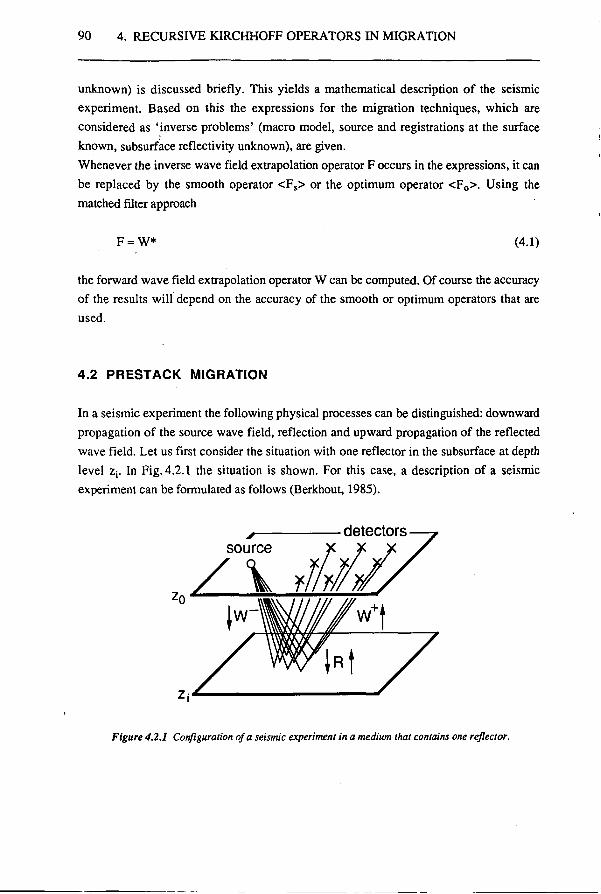
90 4. RECURSIVE KIRCHHOFF OPERATORS IN MIGRATION
unknown) is discussed briefly. This yields a mathematical description of the seismic experiment. Based on this the expressions for the migration techniques, which are considered as 'inverse problems' (macro model, source and registrations at the surface known, subsurface reflectivity unknown), are given. Whenever the inverse wave field extrapolation operator F occurs in the expressions, it can be replaced by the smooth operator <FS> or the optimum operator <F0>. Using the matched filter approach
F = W* (4.1)
the forward wave field extrapolation operator W can be computed. Of course the accuracy of the results will depend on the accuracy of the smooth or optimum operators that are used.
4.2 PRESTACK MIGRATION
In a seismic experiment the following physical processes can be distinguished: downward propagation of the source wave field, reflection and upward propagation of the reflected wave field. Let us first consider the situation with one reflector in the subsurface at depth level z;. In Fig. 4.2.1 the situation is shown. For this case, a description of a seismic experiment can be formulated as follows (Berkhout, 1985).
detectors -
Figure 4.2.1 Configuration of a seismic experiment in a medium that contains one reflector.
4.2 PRESTACK MIGRATION 91
1'. Forward extrapolation of the downgoing source wave field S+ from the surface ZQ to depth level Zj:
S+(x,y,zi>a)) = W+(x,y,Az;,k) * S+(x,y)Zo,co), (4.2)
with AZJSZJ-ZQ, ZJ>Z0, Remember that the symbol * denotes a two-dimensional, space dependent, spatial convolution along the x- and y-coordinate. 2. Reflection at depth level Zj which causes an upgoing reflected wave field:
P^x.y.Zi.co) = R(x,y,Zi,co) * S^x.y.Zj.co), (4.3a)
where R is a reflection function which describes the angle-dependent reflectivity. In the special case that the incident wave field S+ is locally plane, reflection function R reduces to a reflection coefficient and hence the space dependent spatial convolution in eq. (4.3a) may be replaced by a multiplication:
Pj-(x,y,Zi,co) = Rj(x,y,zi,co)Sj+(x,y,zi,(o). (4.3b)
The subscript j is related to the shot position at the surface. Note that it indicates the orientation of the locally plane source field. 3. Forward extrapolation of the upgoing reflected wave field from depth level z; to the surface ZQ:
Pj-(x,y,z0,co) = W-(x,y,AZi,k) * Pjlx.y.Zj.co). (4.4)
In practice there is reflectivity at all depth levels in the subsurface. Therefore these three steps should be repeated for all depth levels in the subsurface up to the maximum depth of interest. Because a seismic experiment is band-limited, the true broad-band reflectivity of the 'real world' can never be recovered. For our computations we therefore may replace it by a discrete, band-limited reflectivity. In that case the interval Az between depth levels z;
and Zj_! should satisfy: Az< X/2. Note that this limits the number of depth levels to be taken into account In the formulation of a seismic experiment according to eqs.(4.2) to (4.4), it is assumed that the acquisition limitations related to source and detectors have been corrected for.
92 4. RECURSIVE KIRCHHOFF OPERATORS IN MIGRATION
The equations can be combined in the following recursive modeling scheme in which the reflectivity of all depth levels is taken into account:
Pj"(x,y,zi,co)= R(x,y,zi,co)*Sj+(x,y)zi,co) + W_(x,y,Az,k;)*Pj"(x,y)zi+i)0)), for i = M-l, M-2, . . ., 2, 1, 0, (4.5a)
With A z = Z i + 1 - Z ; , Z i + 1 >Z; . ;. ..; .;
In case of a locally plane incident field this equation can be written as ;
Pj"(x,y,2j,0)) = RjCx.y.Zj.o)) Sj+(x,y,Zi,o)) + W-(x,y,Az,k) * Pj^x.y.Zj^co), for i = M-l, M-2, . . . ,2, 1,0. (4.5b)
Note that the computations start at the deepest depth level of interest zM and proceed in the upward direction to the surface ZQ. In this expression the upgoing pressure field at depth level zM is given by
Pj~"(x,y,zM,co)= R(x,y,zM,k)*Sj+(x,y,zM,C0). (4.6)
The source wave field is defined recursively according to
Sj+(x,y,Zi,0)) = W+(x,y ,Az,k) * Sj+(x,y,zi_1 ,co) (4.7)
for i = 1, 2, . . ., M.
Now that we have briefly discussed the forward problem, we continue with the inverse problem: the seismic migration. Each seismic experiment can be migrated individually (Berkhout, 1985 and Wapenaar, 1986). Such a migration basically consists of the following steps. 1. Forward extrapolation of the downgoing source wave field from depth level zt_x to z;
according to eq. (4.7)
S/fr.y.Zi,©) = W+(x,y,Az,k) * S / f r ^ z ^ ü ) ) . (4.8)
2. Inverse extrapolation of the upgoing reflected wave field from depth level z;_j to zf.
4.2 PRESTACK MIGRATION 93
Pj-(x,y,zi,CO) = F-(x>y,Az,k)*Pj-(x,y,zi_1>co). (4.9)
Compare with eq. (4.4). After these two steps, the source wave field as well as the reflected wave field at depth level Z; are known. The relation between these wave fields which is the reflectivity can now be recovered. Usually, in seismic interpretation one is only interested in the average zero-offset reflectivity. This is determined by the following steps. 3. Correlation of the downgoing source wave field and the upgoing reflected wave field, which yields the zero-offset impulse response <Xj> at depth level z;:
<Xj(x,y,Zi,co)> = J-P:"(x,y,z;,co)[S|(x,y,z;,a))]*, (4.10) SJ
where
s? =((s|(x,y,Zi,co) [S^x.y.zi.co)]* dxdy (4.11)
corrects for the transmission losses. Apart from the information about the reflectivity of the current depth level z;, the zero-offset impulse response also contains the influence of all other depth levels, see eq. (4.5b). This is eliminated in the imaging step. 4. Imaging, or, equivalently, selecting the zero time component by summing all frequency components:
<Rj(x,y,Zi)> = — Re £ <Xj(x,y,zi,co)> . (4.12)
The four steps should be applied recursively for all depth levels of interest. The result is a band-limited estimate of the zero-offset reflectivity. Note that this estimate is the result of the migration of a single-shot record. It is therefore called a 'single-fold' zero-offset reflectivity function. 5. The single-fold migration results of all shot records can be summed. This yields the final migration result: a 'multi-fold' band-limited estimate of the zero-offset reflectivity:
<R(x,y,Zi)> = X <Rj(x,y,Zi)> . (4.13) j
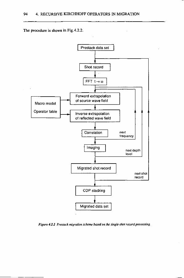
94 4. RECURSIVE KIRCHHOFF OPERATORS IN MIGRATION
The procedure is shown in Fig.4.2.2.
Prestack data set
' 1
Shot record
' ' FFT t->co
Macro model
Operator table
\ r
Forward extrapolation of source wave field
" Inverse extrapolation of reflected wave field
' Correlation
' ' Imaging
■
i
next frequency
i i
next depth level
1
Migrated shot record
'
i l
next shot record
r CDP stacking
1
Migrated data set
Figure 422 Prestack migration scheme based on the single-shot record processing.
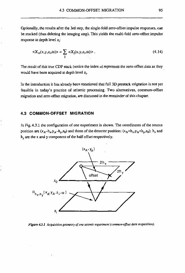
4.3 COMMON-OFFSET MIGRATION 95
Optionally, the results after the 3rd step, the single-fold zero-offset impulse responses, can be stacked (thus deleting the imaging step). This yields the multi-fold zero-offset impulse response at depth level z;:
<Xst(x,y,Zi,co)> = X <Xj(x,y,Zi,(ü) j
>. (4.14)
The result of this true CDP stack (notice the index st) represents the zero-offset data as they would have been acquired at depth level Zj.
In the introduction it has already been mentioned that full 3D prestack migration is not yet feasible in today's practice of seismic processing. Two alternatives, common-offset migration and zero-offset migration, are discussed in the remainder of this chapter.
4.3 COMMON-OFFSET MIGRATION
In Fig. 4.3.1 the configuration of one experiment is shown. The coordinates of the source position are (xA-hx,yA-hy,z0) and those of the detector position: (xA+hx,yA+hy,z0); hx and hy are the x and y component of the half offset respectively.
(xA.yA)
R h x , h y < x A - y A ' z i ^
Figure 4.3.1 Acquisition geometry of one seismic experiment (common-offset data acquisition).
96 4. RECURSIVE KIRCHHOFF OPERATORS IN MIGRATION
Before we give an expression for common-offset migration we first consider the forward case. Like in the previous, section we distinguish three phases in the seismic experiment: downward propagation, reflection and upward propagation. The common-offset experiment can be described as follows. For notational simplicity we consider a laterally invariant medium. 1. The downward extrapolation of the downgoing source wave field from the surface ZQ to depth level z; can be formulated as
S^x.y.zj.co) = W+(x,y,Azi,ü))*S+(x,y,z0,co), (4.15)
with Az; = Zj-z0, Zj>z0. Using • ■ ■ ■ . . ' <
S+(x,y,z0,(ö) = S+(zo,co) 8[(xA-hx)-x,(yA-hy)-y] (4.16)
eq. (4.15) can be written as
S+(x,y,Zi)(0) = S+(z0,co)W+[(xA-hx)-x,(yA-hy)-y, Azj.co]. (4.17)
2. The upward extrapolation of the upgoing reflected wave field from depth level z( to the detector at surface position (xA+hx,yA+hy,z0) is described by
P-(xA+hx,yA+hy,z0,CO) =}{ W-[(xA+hx)-x,(yA+hy)-y,Azi,co] P-(x,y,Zi,ü>) dxdy.
(4.18)
In this equation the upgoing reflected wave field at depth level z; is defined as
p-(x,y,Zi,co) = Rhxihy(x,y,zi,co) S+(x,y,zi,co). (4.19)
Note that we assumed that the reflectivity can be represented by a distribution of reflection coefficients Rhx,hy. see also eq.(4.3b).
With eq. (4.17) and (4.19), eq. (4.18) can be rewritten as
4.3 COMMON-OFFSET MIGRATION 97
P-(xA+hx,yA+hy,zo,co) = S+(zo,co) fJwhxihy(xA-x,yA-y,Azi,co) Rhx,hy(x,y,zi,co) dxdy , (4.20)
where
Whl,hy(xA-x,yA-y,Azi,C0) = (4.21) W-[(xA+hx)-x,(yA+hy)-y,Azi,co] W+[(xA-hx)-x,(yA-hy)-y,Azi)(o].
In practice, the reflections occur at all depth levels, hence, common offset data can be described by
PhI,h/x'yiZo-c°) = S+(z0,co) YJ Whx,hy(x,y,Azi,co) * Rhx,hy(x,y,Zj,co), (4.22) i
for i = 1, 2 , . . ., M,
with
Whx,hy(x,y,Azi,co) = W-(x+hx,y+hy,Azi,CD) W+(x-hx,y-hy,Az;,CD) (4.23) and
Phx,hy(x'v'zo>co) = P"(x+hX)y+hy,z0,Cü). (4.24)
Based on the forward expressions the following migration scheme is proposed. 1. Compute the inverse wave field operator FhXihy for the current depth level. Following the same procedure as in prestack migration, we take the matched filter approach according to
Fhx.hy = Whx,hy, (4.25)
where Whx,hy is given by eq. (4.23). 2. Apply the operator to the common-offset data for all frequency components of interest and image for the current depth level:
<RhI.hy(x,y,zi)> = — Re £ Fhx,hy(x,y,Azi,co) * Phx,hy(x,y,z0,(ü). (4.26)
98 4. RECURSIVE KIRCHHOFF OPERATORS IN MIGRATION
These two steps should be repeated for all depth levels.
For a practical application, common-offset migration is not recommended. This is because the operator Fhx,hy, being the product of two operators, is not a solution of the wave equation. As a consequence the extrapolation can not be formulated recursively. This means that for each depth level new operators must be computed. Hence, the computational cost will be considerable. As we will see in the next section, zero-offset migration (a special case of common-offset migration) does not have this disadvantage if the half-velocity substitution is used.
4.4 ZERO-OFFSET MIGRATION
The zero-offset configuration can be considered as a common-offset configuration where the half offsets hx and hy are taken zero: F),Xihy -* F0 0- According to eqs.(4.23) and (4.25) the inverse extrapolation operator to be used in the migration is given by
F0,o(x,y,Azi,<o) = w£i0(x,y,Azi,<ö) = [w2(x,y,Azi,co)]* . (4.27)
This operator has the same disadvantage as the general common-offset operator (eq. (4.23)): it is not a solution of the wave equation because it is a product of two operators. Therefore, in practice it is approximated by
Fo,o(x,y,Azi,co) - Fzo(x,y,Azi,co) = W*(x,y,Azi,2co). (4.28)
Notice the index zo (zero-offset). It indicates the half-velocity (or double-frequency) substitution that is always used in zero-offset migration (see also section 1.2, the 'exploding reflector' model). The use of F^ instead of F0io causes the incorrect amplitude handling that has already been mentioned in section 1.2. However, the traveltimes are taken into account correctly. A correct treatment of the traveltimes is important for a good recovery of the structural information.
Because F^ is a solution of the wave equation, it can be applied in a recursive way. Hence, vertical as well as lateral velocity variations can be easily handled. The 3D zero-offset migration scheme consists of the following steps.
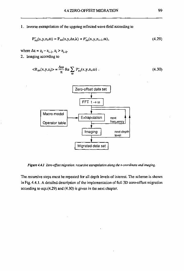
4.4 ZERO-OFFSET MIGRATION 99
1. Inverse extrapolation of the upgoing reflected wave field according to
P^oCx.y'2»03) = Fzo(x,y,Az,k) * PZ0(x,y,Zi_i,a>), (4.29)
where Az = z; - Z;^, z; > z ^ . 2. Imaging according to
<Rzo(x,y,Zi)> = — Re £ Pzo(x,y,zi(ü)) 7 1 <0
(4.30)
Macro model
Operator table
Zero-offset data set
FFT t->co
Extrapolation next frequency
/ . i ,
Imaging next depth level
Migrated data set
Figure 4.4.1 Zero-offset migration: recursive extrapolation along the z-coordinate and imaging.
The recursive steps must be repeated for all depth levels of interest. The scheme is shown in Fig. 4.4.1. A detailed description of the implementation of full 3D zero-offset migration according to eqs.(4.29) and (4.30) is given in the next chapter.
' : .' •'• ''f 1 0 1
CHAPTER 5
COMPUTATIONAL ASPECTS OF FULL 3D ZERO-OFFSET MIGRATION
5.1 INTRODUCTION «?■-
The smooth operator and the optimum operator that have been discussed in chapter 3 can be used in various seismic processing techniques that are based on wave field extrapolation. In chapter 4 the emphasis was on migration techniques. Aspects concerning the actual implementation of a full 3D, table driven, zero-offset migration algorithm are discussed in this chapter. First, a detailed scheme of the structure of this algorithm is given. It is used to explain the data organization, the requirements with respect to the capacity of disk and core memory of the computer, the I/O, etc. Next, the implementation of the extrapolation is discussed. The extrapolation is the most important part of the migration scheme. This holds for the accuracy as well as for the efficiency of the algorithm. Furthermore,, we give an expression for the number of floating point (fp-) operations of our migration scheme and compare this with the number of fp-operations of the reverse-time migration scheme as discussed by Chang and McMechan (1989). A cost comparison between these methods is also made for the core memory requirements. Finally, we discuss the results of some benchmarks. We run several tests on the following vector computers: Convex Cl and C2, Cray X-MP and Alliant 4CE. The latter one also has the possibility for parallel processing.
5.2 STRUCTURE OF THE 3D TABLE-DRIVEN ZERO-OFFSET MIGRATION ALGORITHM
A flow-chart of the 3D table-driven zero-offset migration algorithm is given in Fig. 4.4.1. The formulas for the recursive extrapolation and imaging, eq. (4.28) and eq. (4.29) are repeated. The downward inverse extrapolation of the upgoing reflected waves is given by
Pzo(x,y,Zj,co) = FZ0(x,y,Az,k) * Pzo(x,y,zi_1,co) (5.1)
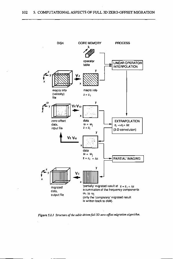
102 5. COMPUTATIONAL ASPECTS OF FULL 3D ZERO-OFFSET MIGRATION
DISK CORE MEMORY k
operator table
^ ?^3? m Vz
^
y \S1
macro info (velocity) file
macro info Z = ZL
CO
rf rf J^ r
VzVc
zero-offset data, input file
data CO = CO:
1 Vz Vco
data CO = CO:
Z = Z | + A Z
Vz
PROCESS
LINEAR OPERATOR INTERPOLATION
EXTRAPOLATION Zj - ) Z j + AZ
(2-D convolution)
'PARTIAL' IMAGING
migrated data, output file
'partially' migrated result at z = z j + Az a summation of the frequency components M l t o COj
(only the 'completely' migrated result is written back to disk).
Figure 5.2.1 Structure of the table-driven full 3D zero-offset migration algorithm.
5.2 STRUCTURE OF 3D ZERO-OFFSET MIGRATION ALGORITHM 103
and the imaging step by
<Rzo(x,y,zi)> = - ^ Re £ Pz0(x>y>zi,ü)) . (5.2)
These steps are repeated recursively for all depth levels. A detailed picture that shows the structure of the algorithm is shown in Fig. 5.2.1. The three 'columns' of the figure represent the disk memory space, the core memory space and the processing steps that are performed by the algorithm respectively. A description is given now.
Data flow We start with a Fourier transformed zero-offset data set (x,y,co domain), stored in a file on disk. A table containing a set of 'smoothed' or 'optimized' wave field extrapolation operators must be available in core memory. A file containing the macro model velocity information must be present on disk. It is possible to use this file also as output file for the migrated result. This means a reduction of the required disk space. However, in that case the original velocity information will get lost. Depth loop
- A 2D x,y panel, depth level z=Z;, containing the macro model velocity information, c(x,y,Zi), of the current depth level z; is read from the macro model file on disk and stored in core memory. The extrapolation from the current depth level to the next, Z; -» z;+Az, can now be performed.
Frequency loop - A monochromatic 2D x,y data panel, depth level z=z; and frequency component
C0=C0j, is read from the zero-offset data file on disk and stored in core memory. X,Y loop
- The local wavenumber value at position (x,y,z;) is determined: k = (Dj/c(x,y,zi).
- Only if this value differs from the previous one, a new operator for this wavenumber value is computed by means of linear interpolation between two operators from the table.
- The operator is applied to the data (see section 5.4). End ofX.Y loop
104 5. COMPUTATIONAL ASPECTS OF FULL 3D ZERO-OFFSET MIGRATION
Once all points have been extrapolated, the result is a monochromatic 2D x,y data panel at depth level z=z;+Az for frequency component CÜ=CÖJ.
- This panel is written to the zero-offset data file on disk, where it replaces the monochromatic 2D x,y data panel at depth level z = Z; for frequency component CU = C0j.
- Furthermore, this panel is used to carry out a part 'of the imaging step. One does not need to wait until all frequency components have been treated to do the summation. Instead one can simply add the real parts of the extrapolated results for the current frequency component, (0=C0j, to the 'partially' imaged result of the previously treated frequency components C0j to (0:V This yields a partially imaged 2D x,y panel at z=Z;+Az which is the result of a summation of the frequency components Wj to C0j. It is called partial as long as not all frequency components have contributed to the result.
End of frequency loop Once all frequency components have been treated, the output is: 1. the migrated ('fully' imaged) 2D x,y panel at depth level z=z;+Az,
- this panel is written to the output file on disk, 2. a 3D zero-offset data set in the x,y,co domain at depth level z=z;+Az stored in the data file on disk. It will be used as input for the extrapolation to the next depth level.
End of depth loop Once this procedure has been repeated for all depth levels, the result is the migrated data set in the the x,y,z domain.
Some remarks about the algorithm: - According to our experience the speed of the algorithm is never bounded by the I/O from disk to core memory and vice versa. The wave field extrapolation almost completely determines the computation time. - During the migration process we have the extrapolated zero-offset data in the x,y,co domain available as an intermediate result at every depth level. Examination of those 'redatumed' results, after an inverse Fourier transformation to the x,y,t domain, may contribute to a better understanding of the migrated result - The fact that the migrated result is built up gradually, depth level after depth level, offers the possibility of quality control during the process. E.g., a few 'bad' samples in the zero-offset data may ruin the migration result: if they have a large amplitude they cause the so-
5.2 STRUCTURE OF 3D ZERO-OFFSET MIGRATION ALGORITHM 105
called migration smiles. Such problems can be detected in an early stage. Furthermore, the effects of an incorrect macro velocity model like overmigration or undermigration may already become clear during the migration process. - The migration can be easily implemented in a parallel way because the extrapolation is performed per frequency component. Working per frequency component is a natural way of dividing a problem into independent parts, each of which can be treated by a separate processor.
required core memory space According to Fig. 5.2.1 the next amounts of data are kept in core memory: - a 2D x,y panel, z constant, containing macro model velocity information, size:
(numx)(numy) real numbers. - a 2D x,y panel, co constant, containing monochromatic zero-offset data at depth level
z = z;, size: (numx)(numy) complex numbers, or 2(numx)(numy) real numbers.
- a 2D x,y panel, (u constant, containing monochromatic zero-offset data at depth level z = z;+Az, size:
(numx)(numy) complex numbers, or 2(numx)(numy) real numbers.
- a 2D x,y panel, z constant, containing (partially) imaged data, size: (numx)(numy) real numbers.
- a table containing the extrapolation operators, size: (numop)(Nx+l)(Ny+l) complex numbers, or 2(numop)(Nx+l)(Ny+l) real numbers,
numop represents the number of operators in the table. Hence, the core memory must be large enough for the storage of
6(numx)(numy) + 2(numop)(Nx+l)(Ny+l) real numbers. (5.3)
Example. With the next parameters: numx=500, numy= 100, Nx= 12, Ny= 12, a table containing 400 operators and 4 bytes per real number, we find that a core memory of 1.7 Mbyte is sufficient. Note that this number is modest: the computers that are used in the seismic industry at present usually have much more memory.
106 5. COMPUTATIONAL ASPECTS OF FULL 3D ZERO-OFFSET MIGRATION
5.3 FLOATING POINT OPERATION COUNT
The 3D table-driven zero-offset migration algorithm can be divided into three modules: - generation of a table of wave field extrapolation operators, - Fourier transformation of the data from the x.y.t domain to the x.y.co domain, and - the actual migration: linear interpolation of the operators, recursive extrapolation and
imaging.
Although the generation of a table with 'optimized' operators is computationally intensive, we do not include it in the fp-operation count because a table can be used more than once. In the ideal situation one has a number of tables available for the most common acquisition parameters. The computational cost of the Fourier transformation can be neglected with respect to the cost of the actual migration. Therefore, we concentrate on the fp-operation count of the migration and pay attention to the operator interpolation, the extrapolation and the imaging step respectively.
fp-operation count of the linear interpolation of operators The linear operator interpolation is formulated as:
FM(nx,ny,Az,k) = ( ( " k + ^ k ~ k ) F„(nx,ny,Az,nkAk) + (5.4)
[ ~ ^ F20(nx,ny,Az,(nk+l)Ak),
for nx = 0, 1, 2 , . . ., Nx, and ny = 0, 1, 2, . . ., Ny.
Here, nk is defined as the integer part of the ratio k/Ak. The number of fp-operations of the operator interpolation is
2(NX+1)(N +1) multiplications of a complex number by a real number and (Nx+l)(Ny+l) complex additions, or 6(Nx+l)(Ny+l) fp-operations.
(A multiplication of a complex number by a real number is equivalent to two real multiplications, one complex addition is equivalent to two real additions).
5.3 FLOATING POINT OPERATION COUNT 107
In the migration algorithm, the number of fp-operations for the operator interpolation is not a fixed number. It depends on the structure of the macro model. For one monochromatic extrapolation step it is somewhere in between
no fp operations, for a homogeneous macro model and (5.5) 6(numx)(numy)(Nx+l)(Ny+l) fp-operations for a fully inhomogeneous model.
In a practical macro subsurface model there will be large homogeneous areas. We therefore neglect the contribution of the operator interpolation to the computational cost of the algorithm.
fp-operation count for the extrapolation One monochromatic extrapolation step can be formulated as (see also eq. (3.24)):
N, Ny
Pzo(nx,ny,zi+i,co) = £ X 4 s(nx,ny) Fzotn'x.ny.Az.kfax.ny.zi.co)] (5.6) nj=0 n^=0
{ PZo[(nx-nx),(ny-n'y),Zi,cü] +
PZo[(nx-nx),(ny+ny),Zi,co] +
Pzo[(nx+nx),(ny-ny),Zi,0)] + PzotOix+nxMny+ny^Zi.cü] }AxAy.
for nx = 1, 2 , . . ., numx, and ny = 1, 2 , . . ., numy.
In this expression the symmetry properties of the operator (see eq. (3.23)) have already been included. Application of eq. (5.6) involves
4(numx)(numy)(Nx+l)(Ny+l) complex additions and (numx)(numy)(Nx+l)(Ny+l) complex multiplications, or, 14(numx)(numy)(Nx+l)(Ny+l) fp-operations. (5.7)
(One complex multiplication is equivalent to four real multiplications and two real additions).
We remark that a result like this should be interpreted with care, because it does not take into account the computer architecture (scalar versus vector, add multiply overlap, parallel processing, etc.). However, the fp-operation count is considered as a satisfactory tool to compare algorithms.
108 5. COMPUTATIONAL ASPECTS OF FULL 3D ZERO-OFFSET MIGRATION
The number of fp-operations in expression (5.7) can be reduced by splitting eq. (5.6) into two parts as follows:
N, Ny
Pio(nx,ny,zi+1)co) = X X 4 s(n'x>ny) Fzo[n'x,ny,Az,k(nx,ny,Zi,to)] (5.8)
{ Pzo[(nx-n'x),(ny-ny),Zi,ü)] +
Pz o[(nx-n'x),(ny+ny),Zi,co] }AxAy, for nx = 1, 2 , . . ., numx, and ny = 1,2;. . ., numy.
In this equation Pzo is defined as
PZ0[(nx-nx),ly,Zi,Cö] = Pzo[(nx-nx),ly,Zi,(ü] + Pzo[(nx+nx),ly,Zj,Cu], (5.9)
for ly = 1, 2, . .., numy, and n'x = 0, 1, . . ., Nx.
First the summation according to eq. (5.9) is carried out. This yields
(numy)(Nx+l) complex additions.
This number can be neglected with respect to the number of fp-operations in the application of eq. (5.8). This is given by
2(numx)(numy)(Nx+l)(Ny+l) complex additions and (numx)(numy)(Nx+l)(Ny+l) complex multiplications, or, together 10(numx)(numy)(Nx+l)(Ny+l) fp-operations. (5.10)
Compared with the number in expression (5.7) the number of fp-operations in (5.10) is reduced by about 30%.
fp-operation count for the imaging step The number of fp-operations of a 'partial' imaging step amounts to
(numx)(numy) real additions or fp-operations. (5.11)
5.4 EFFICIENT EMPLEMENTATION OF THE EXTRAPOLATION 109
Note that this number is very small, usually smaller than 0.1% of the number in expression (5.10). The contribution of the imaging step to the fp-operation count is therefore neglected.
Thus, a global estimate of the total number of fp-operations of the migration scheme can be obtained by multiplying the number of fp-operations in expression (5.10) by the number of frequency components, numf, and the number of extrapolation steps, numz:
10(numf)(numz)(numx)(numy)(Nx+l)(Ny+l) fp-operations, (5.12)
The number according to (5.12) is used in the presentation of the benchmark results that are presented in section 5.6. Furthermore, it is used for comparison with a reverse-time migration algorithm, see section 5.5.
5.4 EFFICIENT IMPLEMENTATION OF THE EXTRAPOLATION
The number of fp-operations as given in the previous section is independent of the computer architecture. Only with additional information as: what is the degree of vectorization, is the algorithm suitable for parallel processing etc., one can estimate the efficiency of an algorithm for specific hardware. In this section we pay attention to the efficiency aspects of the 3D table-driven zero-offset migration algorithm.
vectorization In general one can state: the longer a certain 'do-loop', the more efficient it is executed on a vector computer (see also section 5.6 on benchmarks). In a regular implementation of the 2-D convolution along x and y, according to eq. (5.8) and (5.9), a compiler will vectorize either the loop in the x-direction or the loop in the y-direction. The reason is that for vectorization, the stride (the increment between the array elements to be processed) must be constant (or sometimes even preferably one). The elements of the operator are indeed sequentially stored in memory. Unfortunately, for the data this is not the case, as can be seen in Fig. 5.4.1. Another problem arises when the symmetry properties of the operator are incorporated. In that case four quadrants of data must be summed before the operator can be applied, and
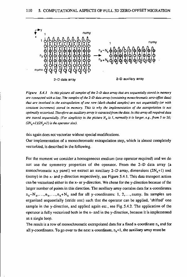
110 5. COMPUTATIONAL ASPECTS OF FULL 3D ZERO-OFFSET MIGRATION
2-D data array 2-0 auxiliary array
Figure 5.4.1 In this picture all samples of the 2-D data array that are sequentially stored in memory are connected with a line. The samples of the 2-D data array (containing monochromatic zero-offset data) that are involved in the extrapolation of one row (dark-shaded samples) are not sequentially (or with constant increment) stored in memory. This is why the implementation of the extrapolation is not optimally vectorized. Therefore an auxiliary array is extracted from the data. In this array all required data are stored sequentially. (For simplicity in the picture Nx is 1, normally it is larger, e.g., from 5 to 20; (2Nx+l)(2Ny+l) is the operator size).
this again does not vectorize without special modifications. Our implementation of a monochromatic extrapolation step, which is almost completely vectorized, is described in the following.
For the moment we consider a homogeneous medium (one operator required) and we do not use the symmetry properties of the operator. From the 2-D data array (a monochromatic x,y panel) we extract an auxiliary 2-D array, dimensions (2NX+1) and (numy) in the x- and y-direction respectively, see Figure 5.4.1. This data transport action can be vectorized either in the x- or y-direction. We chose for the y-direction because of the larger number of points in this direction. The auxiliary array contains data for x-coordinates n x -N x , . . . ,n x , . . . ,n x +N x and for all y-coordinates: 1, 2,...,numy. Its samples are organized sequentially (stride one) such that the operator can be applied, 'shifted' one sample in the y-direction, and applied again etc., see Fig. 5.4.2. The application of the operator is fully vectorized both in the x- and in the y-direction, because it is implemented as a single loop. The result is a row of monochromatic extrapolated data for a fixed x-coordinate nx and for all y-coordinates. To go over to the next x-coordinate, nx+l, the auxiliary array must be
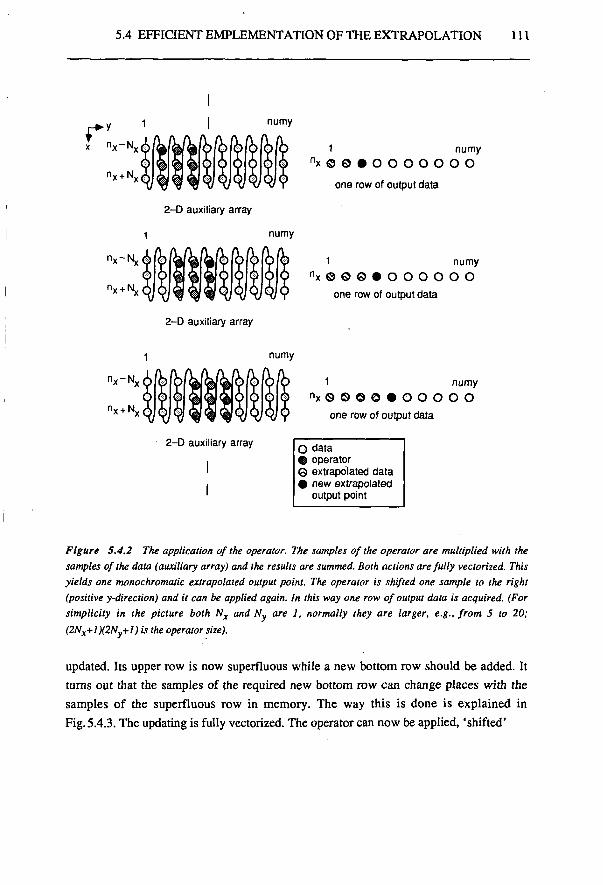
5.4 EFFICIENT EMPLEMENTATION OF THE EXTRAPOLATION 111
r: x n x_ N x
riv + N. x + ™x
numy
2-D auxiliary array
numy
2-D auxiliary array
1 numy nx © © # 0 0 0 0 0 0 0
one row of output data
1 numy n x © 0 0 » O O O O O O
one row of output data
numy
2-D auxiliary array
I
1 numy n x 0 © © 0 « 0 0 0 0 0
one row of output data
O data @ operator O extrapolated data 9 new extrapolated
output point
Figure S.4.2 The application of the operator. The samples of the operator are multiplied with the samples of the data (auxiliary array) and the results are summed. Both actions are fully vectorized. This yields one monochromatic extrapolated output point. The operator is shifted one sample to the right (positive y-direction) and it can be applied again. In this way one row of output data is acquired. (For simplicity in the picture both Nx and Ny are 1, normally they are larger, e.g., from 5 to 20; (2Nx+l)(2Ny+l) is the operator size).
updated. Its upper row is now superfluous while a new bottom row should be added. It turns out that the samples of the required new bottom row can change places with the samples of the superfluous row in memory. The way this is done is explained in Fig. 5.4.3. The updating is fully vectorized. The operator can now be applied, 'shifted'
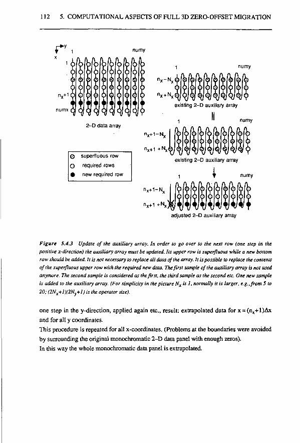
112 5. COMPUTATIONAL ASPECTS OF FULL 3D ZERO-OFFSET MIGRATION
© required rows # new required row
adjusted 2-D auxiliary array
Figure 5.4.3 Update of the auxiliary array. In order to go over to the next row (one step in the positive x-direction) the auxiliary array must be updated. Its upper row is superfluous while a new bottom row should be added. It is not necessary to replace all data of the array. It is possible to replace the contents of the superfluous upper row with the required new data. The first sample of the auxiliary array is not used anymore. The second sample is considered as the first, the third sample as the second etc. One new sample is added to the auxiliary array. (For simplicity in the picture Nxis 1, normally it is larger, e.g., from 5 to 20; (2Nx+l)(2Ny+l) is the operator size).
one step in the y-direction, applied again etc., result: extrapolated data for x = (nx+l)Ax and for all y coordinates. This procedure is repeated for all x-coordinates. (Problems at the boundaries were avoided by surrounding the original monochromatic 2-D data panel with enough zeros). In this way the whole monochromatic data panel is extrapolated
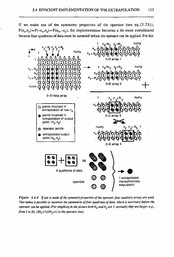
5.4 EFFICIENT EMPLEMENTATION OF THE EXTRAPOLATION 113
If we make use of the symmetry properties of the operator (see eq. (3.23)), F(nx>ny) = F(-nxlny)=F(nx,-ny), the implementation becomes a bit more complicated because four quadrants of data must be summed before the operator can be applied. For the
f*y 1 V ' P / ^ 1 ny-Ny
numy
n x -N .
nx + N,
numx
2-D data array
O points involved in extrapolation of row nx
© points involved in extrapolation of output point (rix.ny)
@ operator points
0 extrapolated output point (r^.ny)
2-D array 1
1 ny-Ny ry+Ny
n x -N .
2-D array 2
n y n y + N y
2-D array 3
numy
numy
+ numy
numy ny n y - N y 1
2-D array 4
4 quadrants of data
operator 1 extrapolated monochromatic outputpoint
Figure S.4.4 If use is made of the symmetry properties of the operator, four auxiliary arrays are used. This makes it possible to vectorize the summation of four quadrants of data, which is necessary before the operator can be applied. (For simplicity in the picture both Nx and Ny are I, normally they are larger, e.g., from 5 to 20; (2Nx+l)(2Ny+l) is the operator size).
114 5. COMPUTATIONAL ASPECTS OF FULL 3D ZERO-OFFSET MIGRATION
interested reader the procedure is described next. The implementation is visualized in Figure 5.4.4. First two auxiliary 2-D arrays, called 1 and 2, are extracted from the 2-D data array (monochromatic x,y panel), with sizes (Nx+1) and (numy) in the x- and y-direction respectively. These data transport actions are vectorized in the y-direction. Array 1 contains data for nx ,nx+l,.. . ,nx+Nxand for all y: 1,2 numy. Notation for array 1: (Tnx.Tyjn). Note that the arrows indicate the order of the elements. Array 2 contains data for nx ,nx- l nx-Nx and for all y: 1,2,...,numy: (nxi,Tyall). The sum of array 1 and array 2 (see eq. (5.9)) is stored in array 3: (Tn .Ty,,]!). The summation is fully vectorized. A fourth array is constructed, containing the contents of array 3 in a reorganized way, the y-coordinate is in the reversed order: numy,numy-l,.. . , 1. Notation for array 4: (TnxJ,,yal|.l.). This data transport action is vectorized in the x-direction. Now the preparations are ready and the extrapolation can start. The part with n y ,n y +l , . . . , ny+Ny of array 3 and the part with n y ,n y - l , . . . , ny-Ny of array 4 are summed: (Tnxl,Tny) + (Tnxi,ny.l.) = (Tnx!, tny l) . This summation is fully vectorized The result contains four summed quadrants of data. Then the operator is applied which yields one extrapolated output point. The extrapolation is fully vectorized. Next we 'shift' one sample in the y-direction, sum the involved parts of array 3 and 4: (Tnxi, Tny+U) and apply the operator again, etc. The result is a row of extrapolated data for a fixed x-coordinate nx and for all y coordinates. To go over to the next x-coordinate, nx+l, auxiliary arrays 1 and 2 are updated (fully vectorized) in the same way as was visualized in Figure 5.4.3, and summed (fully vectorized), yielding array 3: (Tnx+li,Tyall). Array 4, the reorganized version of array 3 is constructed (vectorized in 1 direction): (Tnx+U,yai1A). Now the row with x = (nx+l)Ax can be done etc. In this way the whole monochromatic data panel is extrapolated.
If lateral velocity variations are present, an operator must be computed from table operators by linear interpolation. This means that two operators must be multiplied by a scalar and subsequently summed (eq. (5.4)). Both processes fully vectorize.
parallel processing The wave field extrapolation process is performed per frequency component. As mentioned before, working per frequency component offers a natural way of dividing a problem into independent parts, which can be processed separately. Therefore our migration scheme is very well suited for parallel processing.
5.5 COMPARISON WITH REVERSE-TIME MIGRATION 115
5.5 COST COMPARISON WITH REVERSE-TIME MIGRATION
We compare our migration algorithm with the acoustic full 3-D reverse time migration algorithm as discussed by Chang and McMechan (1989). This is done for the number of fp-operations as well as for the required core memory space. As mentioned in section 2.1, the recursive extrapolation in reverse-time migration is performed backwards in time without dip limitations. At each extrapolation step the zero-offset data provide the boundary conditions at the surface. Starting at the maximum registration time, the extrapolation is continued recursively to zero time. The extrapolated section at zero time is the migrated result: all depths are imaged simultaneously. The expression for reverse-time migration, eq. (2.25), is repeated here:
Pk,i.m(tn-At) = 2(l-3a2) pkjl,m(t„) - pk,i,m(t„+At) + (5.13)
+ a2 (Pk+l.l.mOn) + Pk-l,l,m(tn) + Pk.1+1 ,m(tn) + Pk.l-l.mOn) + Pk,l,m+l(tn) + Pk.l,m-1 (tji)) •
where Pk,i,m(tn) *s t n e notation for pZ0(kAxrt,lAyrt,mAzrt,nAt), Axrt= A y ^ A z ^ h is the grid spacing, the index n refers to reverse-time and a = a(x,y,z) = c1/2(x,y,z)At/h.
fp-operation count From eq. (5.13) it follows that the computation of one extrapolated output point requires 9 fp-operations. The total number of fp-operations is found by multiplying this with the number of grid points and the number of time steps numt,.t: ■<
9(numxrt)(numyrt)(numzrt)(numtrt). (5.14)
To be able to compare this result with the one in expression (5.12), one should keep in mind that the spatial and temporal intervals in reverse-time migration are small in order to preclude instability and/or grid dispersion:
nurru^ ~ 5 numx, numyrt ~ 5 numy, (5.15) numz,, = 5 numz, numtj, = 5 numt» 20 numf.
116 5. COMPUTATIONAL ASPECTS OF FULL 3D ZERO-OFFSET MIGRATION
Using this we find for the total number of fp-operations in reverse-time migration
22,500 (numx)(numy)(numz)(numf). (5.16)
This is in the order of ten times larger than the number of fp-operations in table-driven migration (expression (5.12)).
required core memory space Preferably the total data volumes at three consecutive times, t„_j, t„ and t„+1 should be kept in core memory. However, it is possible to replace the data at time t„+1 with the reverse-time extrapolated data at time Vi- Furthermore, the macro model velocity information should be present. Hence, the required core memory space for reverse-time migration is: - a 3D x,y,z volume containing macro model velocity information, size:
(numxrt)(numyIt)(numzrt) real numbers and - two 3D x,y,z volumes containing data at two times, size:
2(numxIt)(numyrt)(numzrt) real numbers.
Hence, unless an huge amount of I/O is accepted, the core memory space must be large enough for
3(numxrt)(numyrt)(numzrt) real numbers, or 375(numx)(numy)(numz) real numbers. (5.17)
Example. With the next parameters: numx = 500, numy = 100, numz = 150 and 4 bytes per real number, we find that the reverse-time migration requires a core memory of more than 10 Gbyte. This number should be compared with the 1.7 Mbyte that is required by table-driven migration (see section 5.4). Note that 10 Gbyte is too much for an implementation on present computers.
5.6 BENCHMARKS
The table-driven migration algorithm was tested on several computers: a Convex Cl, a Convex C2, a Cray X-MP and and an Alliant 4CE. All computers are vector computers.
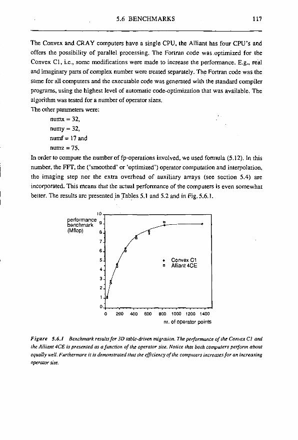
5.6 BENCHMARKS 117
The Convex and CRAY computers have a single CPU, the Alliant has four CPU's and offers the possibility of parallel processing. The Fortran code was optimized for the Convex Cl, i.e., some modifications were made to increase the performance. E.g., real and imaginary parts of complex number were treated separately. The Fortran code was the same for all computers and the executable code was generated with the standard compiler programs, using the highest level of automatic code-optimization that was available. The algorithm was tested for a number of operator sizes. The other parameters were:
numx = 32, numy = 32, numf = 17 and numz = 75.
In order to compute the number of fp-operations involved, we used formula (5.12). In this number, the FFT, the ('smoothed' or 'optimized') operator computation and interpolation, the imaging step nor the extra overhead of auxiliary arrays (see section 5.4) are incorporated. This means that the actual performance of the computers is even somewhat better. The results are presentedin Tables 5.1 and 5.2 and in Fig.5.6.1.
1 0 -performance . benchmark ■ (Mflop) 8 .
7. 6. 5. 4 3.
2 U
0 200 400 600 800 1000 1200 1400 nr. of operator points
Figure 5.6.1 Benchmark results for 3D table-driven migration. The performance of the Convex Cl and the Alliant 4CE is presented as a function of the operator size. Notice that both computers perform about equally well. Furthermore it is demonstrated that the efficiency of the computers increases for an increasing operator size.
Convex C1 Alliant 4CE
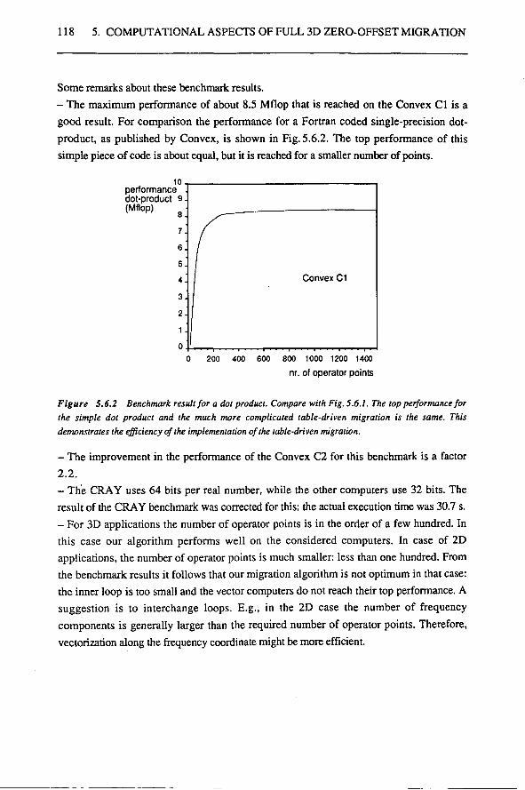
118 5. COMPUTATIONAL ASPECTS OF FULL 3D ZERO-OFFSET MIGRATION
Some remarks about these benchmark results. - The maximum performance of about 8.5 Mflop that is reached on the Convex Cl is a good result. For comparison the performance for a Fortran coded single-precision dot-product, as published by Convex, is shown in Fig. 5.6.2. The top performance of this simple piece of code is about equal, but it is reached for a smaller number of points.
10 performance . dot-product 9-(Mflop) 8 .
200 400 600 800 1000 1200 1400 nr. of operator points
Figure 5.6.2 Benchmark result for a dot product. Compare with Fig. 5.6.1. The top performance for the simple dot product and the much more complicated table-driven migration is the same. This demonstrates the efficiency of the implementation of the table-driven migration.
- The improvement in the performance of the Convex C2 for this benchmark is a factor 2.2. - The CRAY uses 64 bits per real number, while the other computers use 32 bits. The result of the CRAY benchmark was corrected for this: the actual execution time was 30.7 s. - For 3D applications the number of operator points is in the order of a few hundred. In this case our algorithm performs well on the considered computers. In case of 2D applications, the number of operator points is much smaller: less than one hundred. From the benchmark results it follows that our migration algorithm is not optimum in that case: the inner loop is too small and the vector computers do not reach their top performance. A suggestion is to interchange loops. E.g., in the 2D case the number of frequency components is generally larger than the required number of operator points. Therefore, vectorization along the frequency coordinate might be more efficient.
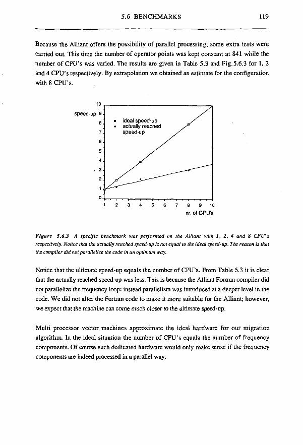
5.6 BENCHMARKS 119
Because the Alliant offers the possibility of parallel processing, some extra tests were carried out. This time the number of operator points was kept constant at 841 while the number of CPU's was varied. The results are given in Table 5.3 and Fig. 5.6.3 for 1, 2 and 4 CPU's respectively. By extrapolation we obtained an estimate for the configuration with 8 CPU's.
1 0 T speed-up 9-
8 .
7 .
6.
5.
4^
. 3 .
2.
1 \
- i — ■ — i — ■ — i — • — i — ■ — i — i — i — > — i — i — i — i — i — i — i
1 2 3 4 5 6 7 8 9 10
nr. of CPU's
Figure 5.6.3 A specific benchmark was performed on the Alliant with 1, 2, 4 and 8 CPU's respectively. Notice that the actually reached speed-up is not equal to the ideal speed-up. The reason is that the compiler did not parallelize the code in an optimum way.
Notice that the ultimate speed-up equals the number of CPU's. From Table 5.3 it is clear that the actually reached speed-up was less. This is because the Alliant Fortran compiler did not parallelize the frequency loop: instead parallelism was introduced at a deeper level in the code. We did not alter the Fortran code to make it more suitable for the Alliant; however, we expect that the machine can come much closer to the ultimate speed-up.
Multi processor vector machines approximate the ideal hardware for our migration algorithm. In the ideal situation the number of CPU's equals the number of frequency components. Of course such dedicated hardware would only make sense if the frequency components are indeed processed in a parallel way.
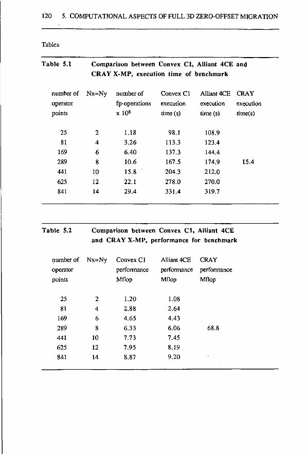
120 5. COMPUTATIONAL ASPECTS OF FULL 3D ZERO-OFFSET MIGRATION
Tables
Table 5.1 Comparison between Convex Cl, Alliant 4CE and CRAY X-MP, execution time of benchmark
number of operator points
25 81
169 289 441 625 841
Nx=Ny
2 4 6 8
10 12 14
number of fp-operations x 108
1.18 3.26 6.40 10.6 15.8 22.1 29.4
Convex Cl execution time (s)
98.1 113.3 137.3 167.5 204.3 278.0 331.4
Alliant 4CE execution time (s)
108.9 123.4 144.4 174.9 212.0 270.0 319.7
CRAY execution time(s)
15.4
Table 5.2 Comparison between Convex Cl, Alliant 4CE and CRAY X-MP, performance for benchmark
number of operator points
25 81
169 289 441 625 841
Nx=Ny
2 4 6 8
10 12 14
Convex Cl performance Mflop
1.20 2.88 4.65 6.33 7.73 7.95 8.87
Alliant 4CE performance Mflop
1.08 2.64 4.43 6.06 7.45 8.19 9.20
CRAY performance Mflop
68.8
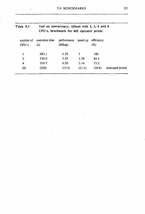
5.6 BENCHMARKS 121
Table 5.3 Test on concurrency, Alliant with 1, 2, 4 and 8 CPU's, benchmark for 841 operator points
number of execution time performance speedup efficiency CPU's (s) (Mflop) (%)
1 2 4 (8)
683.1 530.0 319.7 (220)
4.30 5.55 9.20 (13.4)
1 1.29 2.14 (3.11)
100 64.4 53.2 (38.8) estimated results
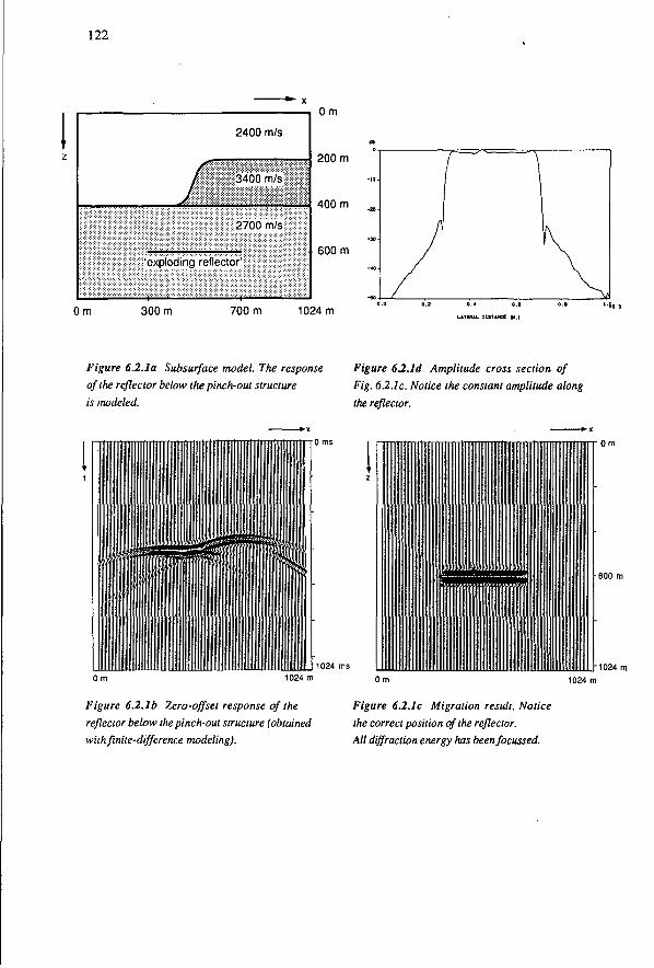
122
■ " X
2400 m/s
J|||BPÖ0m/sl
IIII^IHil^ÉilËlölli^^'"^! l i l l l l l l l l l 'expioding reflector':||||||||
r ¥ ; : ; : ; :W™ : : : : : : : : : : :- ; : : : : ' : : : : : : t : : : : : :™ : a : : ; : : : : : :- : : : :" : : : : : °***vf*>»™vw
Om
200 m
400 m
600 m
0 m 300 m 700 m 1024 m
Figure 6.2.1a Subsurface model. The response Figure 62.1d Amplitude cross section of of the reflector below the pinch-out structure Fig. 6.2.1c. Notice the constant amplitude along is modeled. the reflector.
■WEBS"
>
I O m
1024 m
I I
■ p a w » |l,i,
M I
I I ,
! ' i 1 i i
600 m
M024nt
Figure 6.2.1b Zero-offset response of the Figure 6.2.1c Migration result. Notice reflector below the pinch-out structure (obtained the correct position of the reflector. with finite-difference modeling). All diffraction energy has beenfocussed.
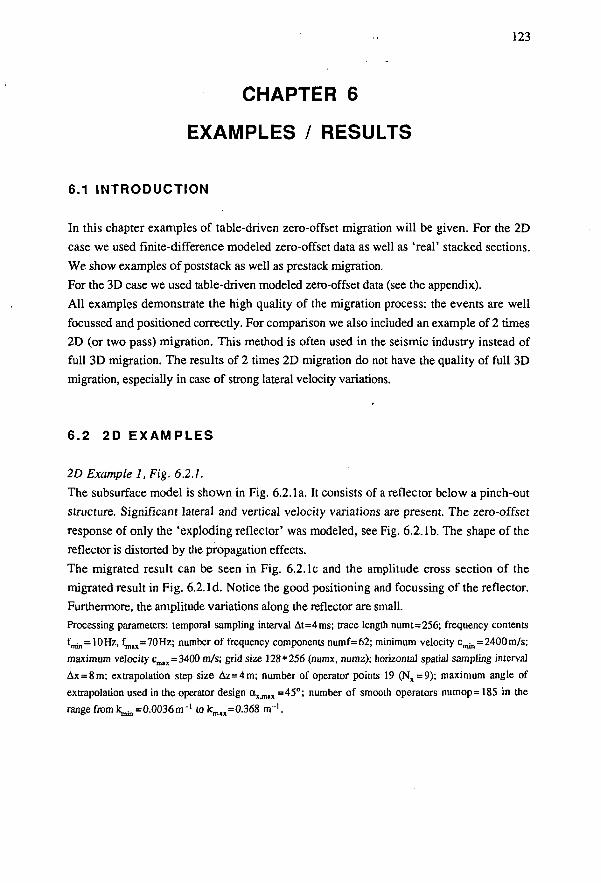
123
CHAPTER 6
EXAMPLES / RESULTS
6.1 INTRODUCTION
In this chapter examples of table-driven zero-offset migration will be given. For the 2D case we used finite-difference modeled zero-offset data as well as 'real' stacked sections. We show examples of poststack as well as prestack migration. For the 3D case we used table-driven modeled zero-offset data (see the appendix). All examples demonstrate the high quality of the migration process: the events are well focussed and positioned correctly. For comparison we also included an example of 2 times 2D (or two pass) migration. This method is often used in the seismic industry instead of full 3D migration. The results of 2 times 2D migration do not have the quality of full 3D migration, especially in case of strong lateral velocity variations.
6.2 2D EXAMPLES
2D Example 1, Fig. 6.2.1. The subsurface model is shown in Fig. 6.2.1a. It consists of a reflector below a pinch-out structure. Significant lateral and vertical velocity variations are present. The zero-offset response of only the 'exploding reflector' was modeled, see Fig. 6.2.1b. The shape of the reflector is distorted by the propagation effects. The migrated result can be seen in Fig. 6.2.1c and the amplitude cross section of the migrated result in Fig. 6.2. Id. Notice the good positioning and focussing of the reflector. Furthermore, the amplitude variations along the reflector are small. Processing parameters: temporal sampling interval At=4ms; trace length numt=256; frequency contents fmin = 10Hz, fma,=70Hz; number of frequency components numf=62; minimum velocity cmin = 2400m/s; maximum velocity cmax=3400 m/s; grid size 128*256 (numx, numz); horizontal spatial sampling interval Ax = 8m; extrapolation step size Az=4m; number of operator points 19 (1^=9); maximum angle of extrapolation used in the operator design axjn„ =45°; number of smooth operators numop= 185 in the range from 1 ^ = 0.0036 nr1 to km„=0.368 rrr1.
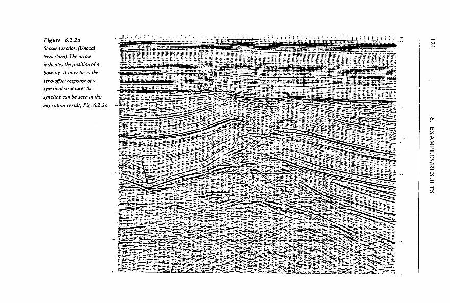
Figure 6.2.2a Stacked section (Unocal Nederland). The arrow indicates the position of a bow-tie. A bow-tie is the zero-offset response of a synclinal structure; the syncline can be seen in the migration result. Fig. 6.2.2c.
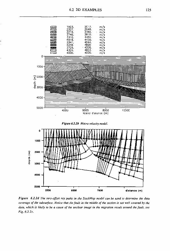
6.2 2D EXAMPLES 125
V777A
rrrm
1923. 2327. 2216. 3746. 3310. 4918. 3341. 4246. 3725. 4324. 4000.
2017. 2048. 2384. 381D. 4494. 4430. 4944. 4890.
■ 4326. 4803. 4000.
m/s m/s m/s m/a m/s m/s m/s m/g m/s m/s m/s
1000
1?2D0O
13000
4000
5000 4000 600O 8000
lateral distance (m) 10000
Figure 6.2.2b Macro velocity model.
1000
2000 -
■o 3000 -
5000 distance (m)
Figure 6.2.2d The zero-offset ray paths in the StackMap model can be used to determine the data coverage of the subsurface. Notice that the fault in the middle of the section is not well covered by the data, which is likely to be a cause of the unclear image in the migration result around the fault, see Fig. 6.2.2c.
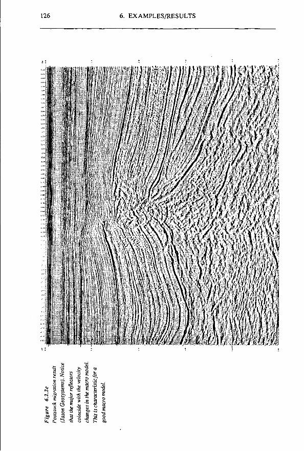
126 6. EXAMPLES/RESULTS
§ s -a
*5 £ B
u
4? s I

6.2 2D EXAMPLES 127
2D Example 2, Fig. 6.2.2 This is a field data example. A stacked section (courtesy of Unocal Nederland) is shown in Fig. 6.2.2a. The macro model was obtained with the use of StackMap® (a software product of Jason Geosystems, which uses stacking information to produce a data-consistent interval-velocity/depth model (Van der Made, 1988)). The model is shown in Fig. 6.2.2b. The migration result is shown in Fig. 6.2.2c. The major reflector boundaries in the migration result coincide with the velocity changes in the macro model. This demonstrates the good quality of the model. Clearly it can be seen that the reflectors in the migration result have moved in the up-dip direction; this property gave migration its name. Furthermore, a bow-tie can be seen in the stacked section (arrow). A bow-tie is the zero-offset response of a synclinal structure as can indeed be seen in the migration result. Notice that the fault in the middle of the migrated section remains rather vague. This can be explained by the fact that this area is not very well covered by the data. The StackMap ray-coverage plot in Fig. 6.2.2d may be used to identify these areas.
2D Example 3, Fig.6.2.3. A stacked section (courtesy of Nederlandse Aardolie Maatschappij) is shown in Fig. 6.2.3a. The macro model (obtained from Delft Geophysical) is shown in Fig. 6.2.3b and the migration result in Fig. 6.2.3c. Especially the fault (arrow) is much clearer determined in the migration result than in the stacked section. Furthermore, a number of small faults can be seen in the low horizontal reflector. If one compares the stack with the migration result, one can see the influence of the macro model on the position of the reflectors. The above mentioned phenomena can even be better observed in the prestack migrated result (obtained from Delft Geophysical), see Fig. 6.2.3d. This is in agreement with the fact that the CMP stacking process yields a low quality 'zero-offset' data. Hence, the prestack migration result will be better than the poststack migration result (see section 1.3). Processing parameters: temporal sampling interval At = 4 ms; trace length numt= 1024; frequency
contents fmin = 10 Hz, fmax = 100 Hz; number of frequency components numf =93; minimum velocity cmin = 1810 m/s; maximum velocity c m a x = 5000 m/s; grid size 472 * 1000 (numx, numz); horizontal
spatial sampling interval Ax = 15 m; extrapolation step size Az = 4 m; number of operator points 75
(Nx = 38); maximum angle of propagation used in the operator design a x m a x = 40°; number of smooth
operators numop = 3641 in the range from k m i n = 0.0251 m - 1 to k m a x = 0.695 m"1.
StackMap® is a registered trademark of Jason Geosystems bv.
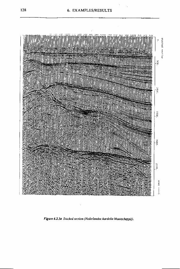
128 6. EXAMPLES/RESULTS
üi
Figure 6.2.3a Stacked section (Nederlandse Aardolie Maatschappij).
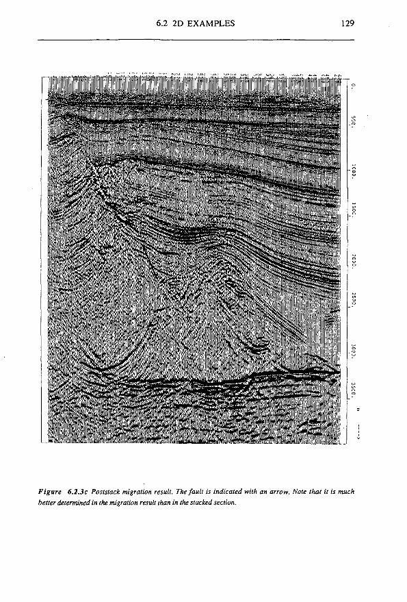
6.2 2D EXAMPLES 129
Figure 6.2.3c Poststack migration result. The fault is indicated with an arrow. Note that it is much better determined in the migration result than in the stacked section.
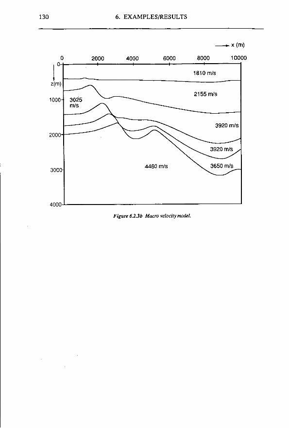
130 6. EXAMPLES/RESULTS
2000 — i —
4000
3000-
4000-
6000 — i —
4460 m/s
8000 1—
-x(m)
10000
1810 m/s
2155 m/s
3920 m/s
3650 m/s
Figure 6.23b Macro velocity model.
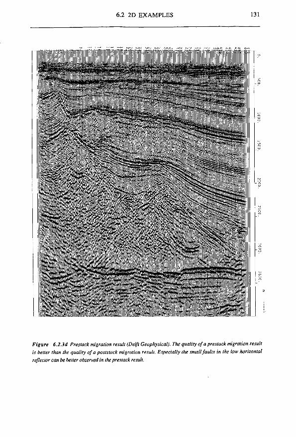
6.2 2D EXAMPLES 131
Figure 6.2.3d Prestack migration result (Delft Geophysical). The quality of a prestack migration result is better than the quality of a poststack migration result. Especially the small faults in the low horizontal reflector can be better observed in the prestack result.
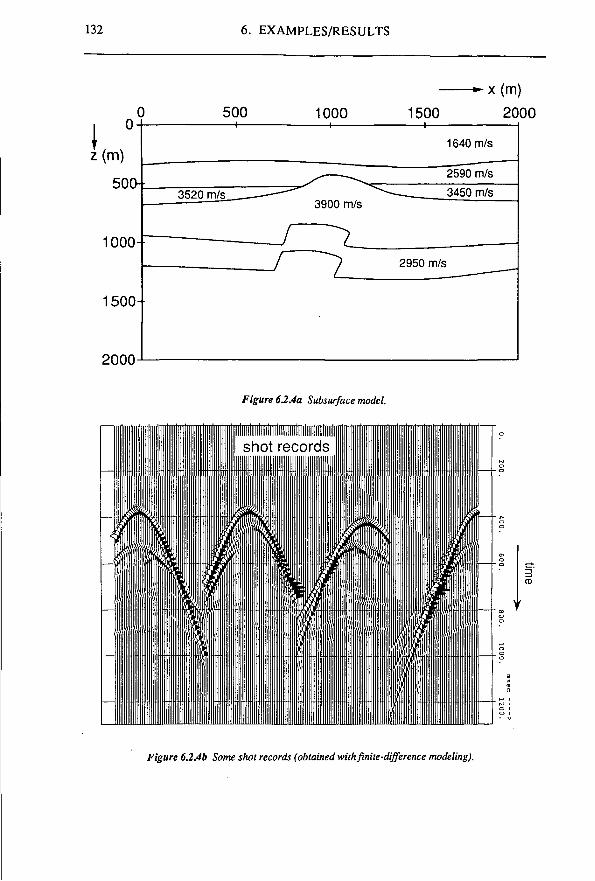
132 6. EXAMPLES/RESULTS
z(m) 50(H_
1000--
1500-
2000-
500 — i —
1000 1
1500
x(m) 2000
1640 m/s
2590 m/s 3450 m/s
2950 m/s
Figure 62.4a Subsurface model.
shot records
Figure 6.2.4b Some shot records (obtained with finite-difference modeling).
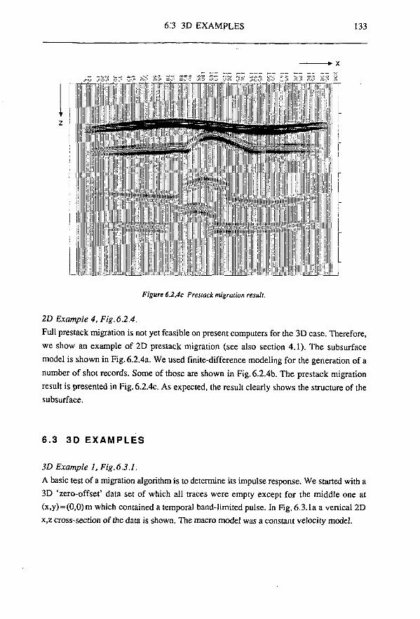
6.3 3D EXAMPLES 133
Figure 6.2.4c Presiack migration result.
2D Example 4, Fig. 6.2.4. Full prestack migration is not yet feasible on present computers for the 3D case. Therefore, we show an example of 2D prestack migration (see also section 4.1). The subsurface model is shown in Fig. 6.2.4a. We used finite-difference modeling for the generation of a number of shot records. Some of those are shown in Fig. 6.2.4b. The prestack migration result is presented in Fig. 6.2.4c. As expected, the result clearly shows the structure of the subsurface.
6.3 3D EXAMPLES
3D Example 1, Fig.6.3.1. A basic test of a migration algorithm is to determine its impulse response. We started with a 3D 'zero-offset' data set of which all traces were empty except for the middle one at (x.y) = (0,0)m which contained a temporal band-limited pulse. In Fig. 6.3.1a a vertical 2D x,z cross-section of the data is shown. The macro model was a constant velocity model.
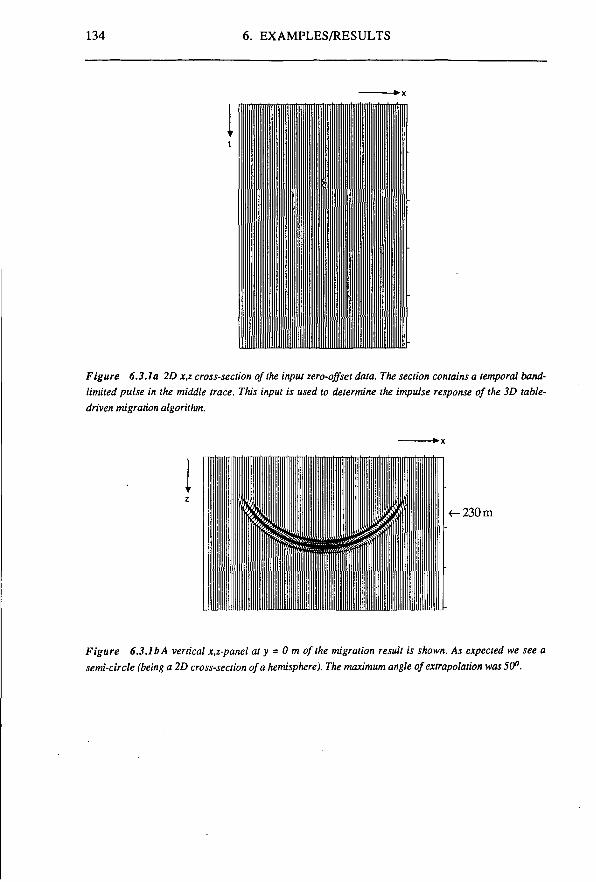
134 6. EXAMPLES/RESULTS
Figure 6.3.1 a 2D x,z cross-section of the input zero-offset data. The section contains a temporal band-limited pulse in the middle trace. This input is used to determine the impulse response of the 3D table-driven migration algorithm.
Figure 6.3.1b A vertical x,z-panel at y = 0 m of the migration result is shown. As expected we see a semi-circle (being a 2D cross-section of a hemisphere). The maximum angle of extrapolation was 50°.
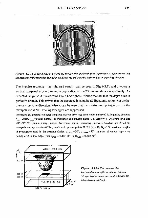
6.3 3D EXAMPLES 135
Figure 6.3.1c A depth slice at z = 250 m. The fact that the depth slice is perfectly circular proves that the accuracy of the migration is good in all directions and not only in the in-line or cross-line direction.
The impulse response - the migrated result - can be seen in Fig. 6.3.1b and c where a vertical x,z-panel at y = 0 m and a depth slice at z = 230 m are shown respectively. As expected the pulse is transformed into a hemisphere. Notice the fact that the depth slice is perfectly circular. This proves that the accuracy is good in all directions, not only in the inline or cross-line direction. Also it can be seen that the maximum dip angle used in the extrapolation is 50°. The higher angles are suppressed. Processing parameters: temporal sampling interval At=4ms; trace length numt= 128; frequency contents fmin = 20Hz, fma„=80Hz; number of frequency components numf=32; velocity c=2000m/s; grid size 90*90*128 (numx, numy, numz); horizontal spatial sampling intervals Ax = 6m and Ay=6m; extrapolation step size Az=6.25m; number of operator points 21*21 (Nx = 10, Ny=10); maximum angles of propagation used in the operator design a x m „ =50°, ax m „ =50°; number of smooth operators numop = 32 in the range from kmin = 0.126 m_1 to k,,,^ = 0.503 m""1.
Figure 6.3.2a The response of a horizontal square reflector situated below a 3D synclinal structure was modeled (with 3D table-driven modeling).
336 m 560 m
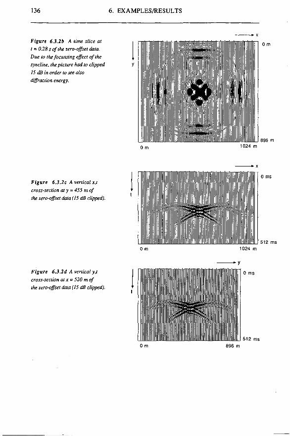
136 6. EXAMPLES/RESULTS
Figure 6.3.2b A time slice at t = 0.28 s of the zero-offset data. Due to the focussing effect of the syncline, the picture had to clipped 15 dB in order to see also diffraction energy.
0 m
896 m 0 m 1024 m
Figure 6.3.2c A vertical x,t cross-section aty = 455 m of the zero-offset data (15 dB clipped).
0 ms
512 ms 0 m 1024 m
Figure 6.3.2d A vertical y,t cross-section alx = 520 m of the zero-offset data (15 dB clipped).
0 ms
I
I I"
I I
I *&**X&S I II ' li "i " l i
i In1 i i i1 i 1 I » ' ' I'1 N
IM I I 'l 512 ms 0 m 896 m
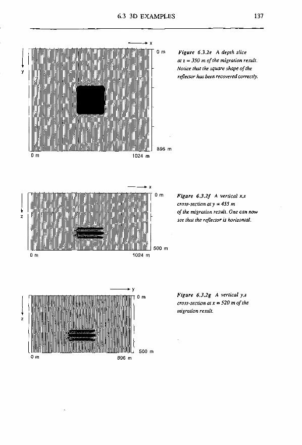
6.3 3D EXAMPLES 137
O m
896 m
Figure 6.3.2e A depth slice at z = 350 m of the migration result. Notice that the square shape of the reflector has been recovered correctly.
O m 1024 m
0 m
500 m
Figure 6.3.2f A vertical x,z cross-section aty = 455 m of the migration result. One can now see that the reflector is horizontal.
0 m 1024 m
0 m
500 m 0 m 896 m
Figure 6.3.2g A vertical y,z cross-section atx = 520 m of the migration result.
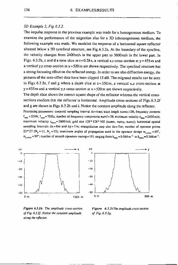
138 6. EXAMPLES/RESULTS
3D Example 2, Fig.6.3.2. The impulse response in the previous example was made for a homogeneous medium. To examine the performance of the migration also for a 3D inhomogeneous medium, the following example was made. We modeled the response of a horizontal square reflector situated below a 3D synclinal structure, see Fig. 6.3.2a. At the boundary of the syncline, the velocity changes from 2400 m/s in the upper part to 3600 m/s in the lower part. In Figs. 6.3.2b, c and d a time slice at t=0.28 s, a vertical x,t cross-section at y=455m and a vertical y,t cross-section at x = 520m are shown respectively. The synclinal structure has a strong focussing effect on the reflected energy. In order to see also diffraction energy, the pictures of the zero-offset data have been clipped 15 dB. The migrated results can be seen in Figs.6.3.2e, f and g where a depth slice at z = 350m, a vertical x,z cross-section at y=455 m and a vertical y,z cross-section at x = 520m are shown respectively. The depth slice shows the correct square shape of the reflector whereas the vertical cross-sections confirm that the reflector is horizontal. Amplitude cross-sections of Figs.6.3.2f and g are shown in Figs. 6.3.2h and i. Notice the constant amplitude along the reflector. Processing parameters: temporal sampling interval At=4ms; trace length numt=128; frequency contents fmin^OH2- fmai=70Hz; number of frequency components numf=28; minimum velocity ^ = 2400 m/s; maximum velocity cm„ = 3600m/s; grid size 128*128*100 (numx, numy, numz); horizontal spatial sampling intervals Ax=8m and Ay=7m; extrapolation step size Az=5m; number of operator points 23*27 (1^ = 11, Ny = 13); maximum angles of propagation used in the operator design a l i m„ =50°, ay,mix = 5 0 ° ; number of smooth operators numop=191 ranging from 1 ^ = 0.069m"1 to km„ = 0.366m"1.
0 m 1024 m 0 m 896 m
Figure 6.3.2h The amplitude cross-section of Fig. 6.3.2f. Notice the constant amplitude along the reflector.
Figure 6.3.2i The amplitude cross-section of Fig. 6.3.2g.
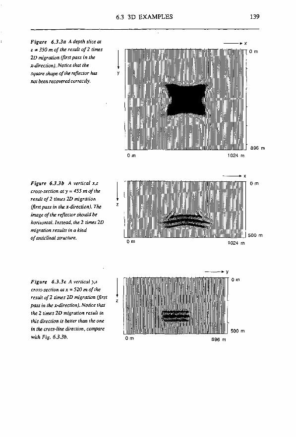
6.3 3D EXAMPLES 139
Figure 6.3.3a A depth slice at z = 350 m of the result of 2 times 2D migration (first pass in the x-direction). Notice that the square shape of the reflector has not been recovered correctly.
0 m
896 m 0 m 1024 m
Figure 6.3.3b A vertical x,z cross-section aty = 455 m of the result of 2 times 2D migration (first pass in the x-direction). The image of the reflector should be horizontal. Instead, the 2 times 2D migration results in a kind of anticlinal structure.
0 m
500 m O m 1024 m
Figure 6.3.3c A vertical y.z cross-section atx = 520 m of the result of 2 times 2D migration (first pass in the x-direction). Notice that the 2 times 2D migration result in this direction is better than the one in the cross-line direction, compare with Fig. 6.3.3b.
0 m
500 m
896 m
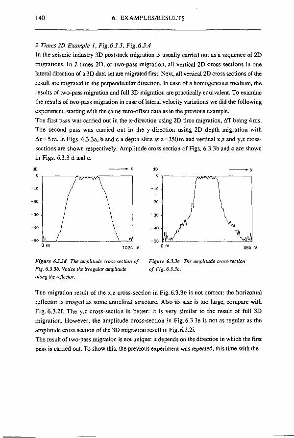
140 6. EXAMPLES/RESULTS
2 Times 2D Example 1, Fig.6.3.3, Fig.6.3.4 In the seismic industry 3D poststack migration is usually carried out as a sequence of 2D migrations. In 2 times 2D, or two-pass migration, all vertical 2D cross sections in one lateral direction of a 3D data set are migrated first. Next, all vertical 2D cross sections of the result are migrated in the perpendicular direction. In case of a homogeneous medium, the results of two-pass migration and full 3D migration are practically equivalent. To examine the results of two-pass migration in case of lateral velocity variations we did the following experiment, starting with the same zero-offset data as in the previous example. The first pass was carried out in the x-direction using 2D time migration, AT being 4 ms. The second pass was carried out in the y-direction using 2D depth migration with Az = 5m. In Figs. 6.3.3a, b and c a depth slice at z = 350m and vertical x,z and y,z cross-sections are shown respectively. Amplitude cross section of Figs. 6.3.3b and c are shown in Figs. 6.3.3 d and e.
o m 1024 m 0 m 896 m
Figure 6.3.3d The amplitude cross-section of Figure 6.3.3e The amplitude cross-section Fig. 6.3.3b. Notice the irregular amplitude of Fig. 6.3.3c. along the reflector.
The migration result of the x,z cross-section in Fig. 6.3.3b is not correct: the horizontal reflector is imaged as some anticlinal structure. Also its size is too large, compare with Fig. 6.3.2f. The y,z cross-section is better: it is very similar to the result of full 3D migration. However, the amplitude cross-section in Fig. 6.3.3e is not as regular as the amplitude cross section of the 3D migration result in Fig.6.3.2i. The result of two-pass migration is not unique: it depends on the direction in which the first pass is carried out. To show this, the previous experiment was repeated, this time with the
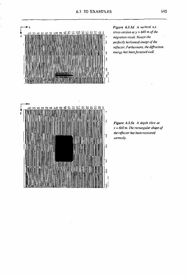
6.3 3D EXAMPLES 145
r Figure 6.3.5d A vertical x,z cross-section at y = 640 m of the migration result. Notice the perfectly horizontal image of the reflector. Furthermore, the diffraction energy has beenfocussed well.
Figure 6.3.5e A depth slice at z = 600 m. The rectangular shape of the reflector has been recovered correctly.

146
147
APPENDIX
NUMERICAL MODELING OF SEISMIC DATA
A.1 INTRODUCTION
For the development and testing of software for seismic processing, realistic synthetic data are required. Data modeled with commercially available ray-tracing software usually do not have the necessary quality for this purpose. This is because ray-tracing is based On a high-frequency approximation of the wave equation. The consequences of this approximation are the inaccurate results in case of caustics, shadow zones, etc. Furthermore, diffraction energy is often not (correctly) incorporated and the problem of 'missing rays' may occur. Accurate results can be obtained with finite-difference modeling based on recursive forward extrapolation along the time coordinate. The expression for forward-time extrapolation is given in eq. (2.25). However, this method is computationally intensive, especially for application in three dimensions. We used finite-difference modeling for the generation of 2D prestack data as well as 2D zero-offset data. In this appendix the emphasis will be on modeling of 3D zero-offset data based on table-driven, recursive forward extrapolation along the depth coordinate. The results of the method are much more accurate than those of ray-tracing while the method requires less computational effort (factor 10) and less computer memory (factor 103) than finite-difference forward-time modeling. Note that equivalent numbers were given in section 5.5 where the cost of reverse-time migration was compared with the cost of table-driven migration. The explanation is that the migration algorithms have a large similarity with the modeling algorithms. This holds for reverse-time migration and forward-time modeling on the one hand and for table-driven migration based on inverse extrapolation and table-driven modeling based on forward extrapolation on the other hand.
Before we go into more detail, we give a 2D example in which the results of the mentioned modeling methods are shown, Fig. A.1. Notice the poor quality of ray-tracing and the high resemblance of the result of table-driven modeling and the result of forward-time modeling, which is considered as a reference.
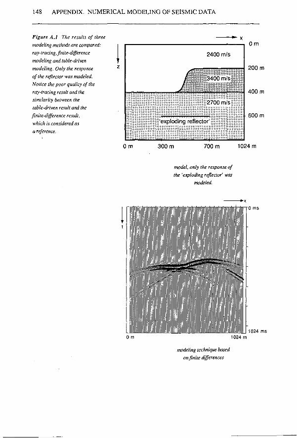
148 APPENDIX. NUMERICAL MODELING OF SEISMIC DATA
Figure A.1 The results of three modeling methods are compared: ray-tracing, finite-difference modeling and table-driven modeling. Only the response of the reflector was modeled. Notice the poor quality of the ray-tracing result and the similarity between the table-driven result and the finite-difference result, which is considered as a reference.
"" X
2400 m/s
ƒ 3400 m/s
2700 m/s
'exploding reflector'
— _ 1 ' i
0m
200 m
400 m
600 m
0 m 300 m 700 m 1024 m
model, only the response of the 'exploding reflector' was
modeled.
0 ms
1024 ms 0 m 1024 m
modeling technique based on finite differences
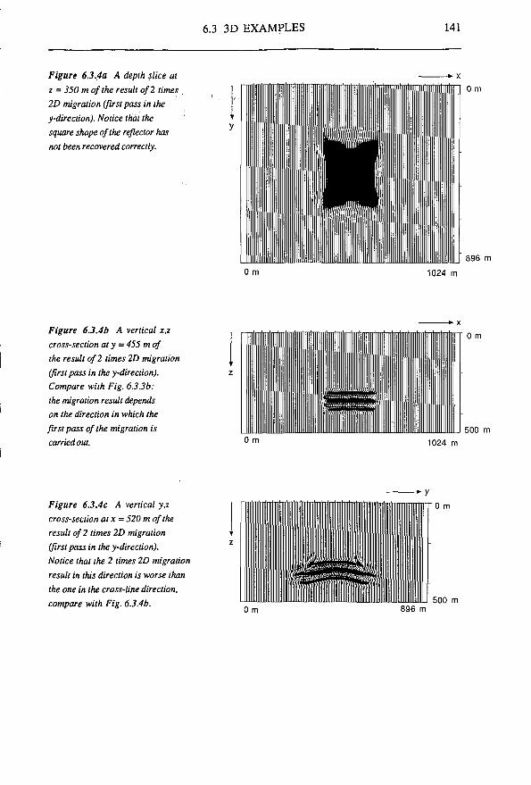
6.3 3D EXAMPLES 141
Figure 6.3.4a A depth slice at z = 350 m of the result of 2 times 2D migration (first pass in the y-direction). Notice that the square shape of the reflector has not been recovered correctly.
0 m
896 m
0 m 1024 m
Figure 6.3.4b A vertical x,z cross-section aty = 455 m of the result of 2 times 2D migration (first pass in the y-direction). Compare with Fig. 6.3.3b: the migration result depends on the direction in which the first pass of the migration is carried out.
0 m
500 m O m 1024 m
Figure 6.3.4c A vertical y,z cross-section atx = 520 m of the result of 2 times 2D migration (first pass in the y-direction). Notice that the 2 times 2D migration result in this direction is worse than the one in the cross-line direction, compare with Fig. 6.3.4b.
0 m
500 m 0 m 896 m
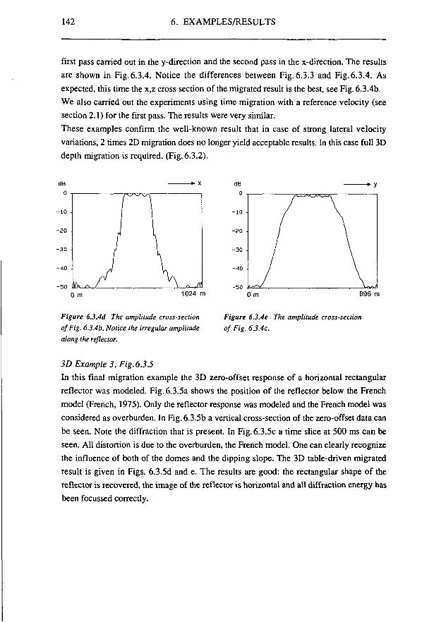
142 6. EXAMPLES/RESULTS
first pass carried out in the y-direction and the second pass in the x-direction. The results are shown in Fig. 6.3.4. Notice the differences between Fig. 6.3.3 and Fig. 6.3.4. As expected, this time the x,z cross section of the migrated result is the best, see Fig. 6.3.4b. We also carried out the experiments using time migration with a reference velocity (see section 2.1) for the first pass. The results were very similar. These examples confirm the well-known result that in case of strong lateral velocity variations, 2 times 2D migration does no longer yield acceptable results. In this case full 3D depth migration is required. (Fig. 6.3.2).
0 m 1024 m 0 m 896 m
Figure 6.3.4d The amplitude cross-section of Fig. 6.3.4b. Notice the irregular amplitude along the reflector.
Figure 6.3.4e The amplitude cross-section of Fig. 6.3.4c.
3D Example 3, Fig. 6.3.5 In this final migration example the 3D zero-offset response of a horizontal rectangular reflector was modeled. Fig. 6.3.5a shows the position of the reflector below the French model (French, 1975). Only the reflector response was modeled and the French model was considered as overburden. In Fig. 6.3.5b a vertical cross-section of the zero-offset data can be seen. Note the diffraction that is present. In Fig. 6.3.5c a time slice at 500 ms can be seen. All distortion is due to the overburden, the French model. One can clearly recognize the influence of both of the domes and the dipping slope. The 3D table-driven migrated result is given in Figs. 6.3.5d and e. The results are good: the rectangular shape of the reflector is recovered, the image of the reflector is horizontal and all diffraction energy has been focussed correctly.
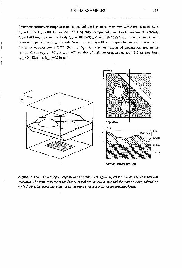
6.3 3D EXAMPLES 143
Processing parameters: temporal sampling interval At=4 ms; trace length numt = 256; frequency contents fmin=10Hz- fmax = 80Hz; number of frequency components numf = 68; minimum velocity c ^ s 1880m/s; maximum velocity cmax = 3800m/s; grid size 192* 128* 120 (numx, numy, numz); horizontal spatial sampling intervals Ax = 6.5 m and Ay = 10m; extrapolation step size Az = 6.5m; number of operator points 21 * 21 (Nx = 10, N = 10); maximum angles of propagation used in the operator design et lm„ =40°, « ï f l l l x = 40o; number of optimum operators numop = 313 ranging from 1 ^ = 0.032 m-1 1 0 ^ = 0.536 m~l.
Figure 6.3.5a The zero-offset response of a horizontal rectangular reflector below the French model was generated. The main features of the French model are the two domes and the dipping slope. (Modeling method: 3D table-driven modeling). A top view and a vertical cross section are also shown.
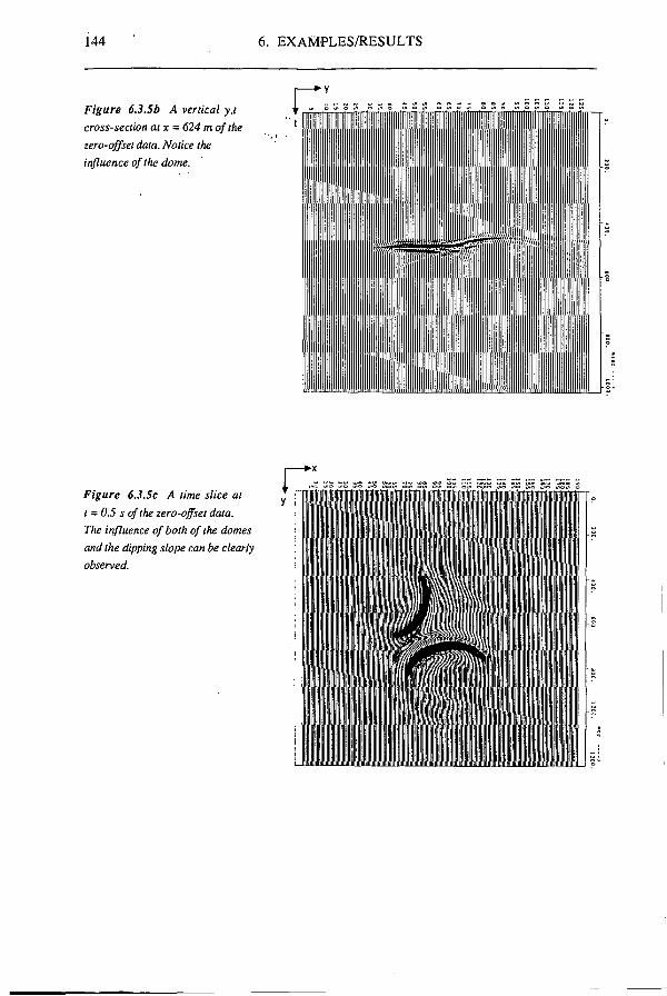
144 6. EXAMPLES/RESULTS
Figure 6.3.5b A vertical y,t cross-section atx = 624 m of the zero-offset data. Notice the influence of the dome.
Figure 6.3.5c A time slice at t = 05 s of the zero-offset data. The influence of both of the domes and the dipping slope can be clearly observed.
r
J
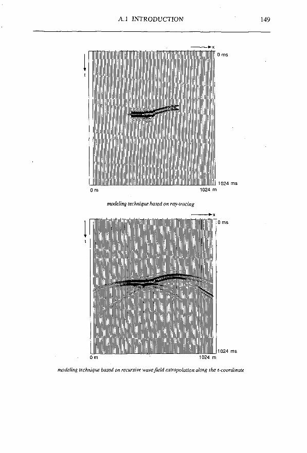
A.1 INTRODUCTION 149
0 ms
1024 ms Om 1024 m
modeling technique based on ray-tracing
0 ms
1024 ms 0 m 1024 m
modeling technique based on recursive wave field extrapolation along the z-coordinate
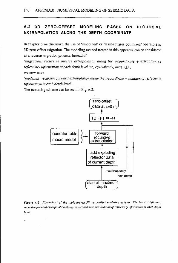
150 APPENDIX. NUMERICAL MODELING OF SEISMIC DATA
A.2 3D ZERO-OFFSET MODELING BASED ON RECURSIVE EXTRAPOLATION ALONG THE DEPTH COORDINATE
In chapter 5 we discussed the use of 'smoothed' or 'least-squares optimized' operators in 3D zero-offset migration. The modeling method treated in this appendix can be considered as a reverse migration process. Instead of 'migration: recursive inverse extrapolation along the z-coordinate + extraction of reflectivity information at each depth level (or, equivalently, imaging)', we now have 'modeling: recursive forward extrapolation along the z-coordinate + addition of reflectivity information at each depth level'. The modeling scheme can be seen in Fig. A.2.
C zero-offset data at z=0 m
operator table macro model
I D F F T w ^ t
forward recursive
extrapolation
add exploding reflector data
of current depth
next frequency
next depth
start at maximum depth 3
Figure A.2 Flow-chart of the table-driven 3D zero-offset modeling scheme. The basic steps are: recursive forward extrapolation along the z-coordinate and addition of reflectivity information at each depth level.
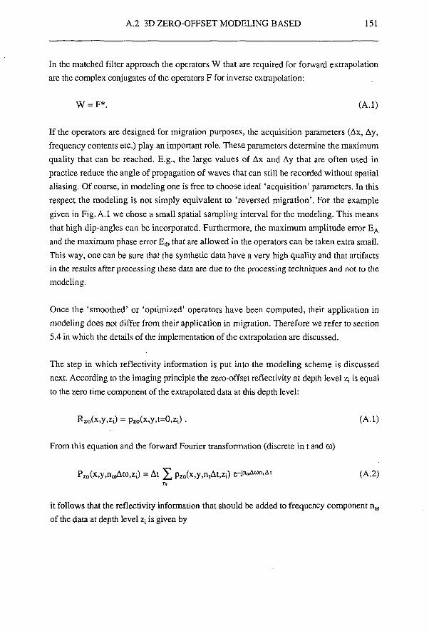
A.2 3D ZERO-OFFSET MODELING BASED 151
In the matched filter approach the operators W that are required for forward extrapolation are the complex conjugates of the operators F for inverse extrapolation:
W = F*. (A.l)
If the operators are designed for migration purposes, the acquisition parameters (Ax, Ay, frequency contents etc.) play an important role. These parameters determine the maximum quality that can be reached. E.g., the large values of Ax and Ay that are often used in practice reduce the angle of propagation of waves that can still be recorded without spatial aliasing. Of course, in modeling one is free to choose ideal 'acquisition' parameters. In this respect the modeling is not simply equivalent to 'reversed migration'. For the example given in Fig. A.l we chose a small spatial sampling interval for the modeling. This means that high dip-angles can be incorporated. Furthermore, the maximum amplitude error EA
and the maximum phase error E<j, that are allowed in the operators can be taken extra small. This way, one can be sure that the synthetic data have a very high quality and that artifacts in the results after processing these data are due to the processing techniques and not to the modeling.
Once the 'smoothed' or 'optimized' operators have been computed, their application in modeling does not differ from their application in migration. Therefore we refer to section 5.4 in which the details of the implementation of the extrapolation are discussed.
The step in which reflectivity information is put into the modeling scheme is discussed next. According to the imaging principle the zero-offset reflectivity at depth level Zj is equal to the zero time component of the extrapolated data at this depth level:
Rzo(x,y,z;) = pzo(x,y,t=0,Zi) . (A.l)
From this equation and the forward Fourier transformation (discrete in t and co)
Pzo(x,y,na)Aco,Zi) = At £ pZ0(x,y,ntAt,Zi) e-i"-40»'^ (A.2) n,
it follows that the reflectivity information that should be added to frequency component nffl
of the data at depth level z; is given by
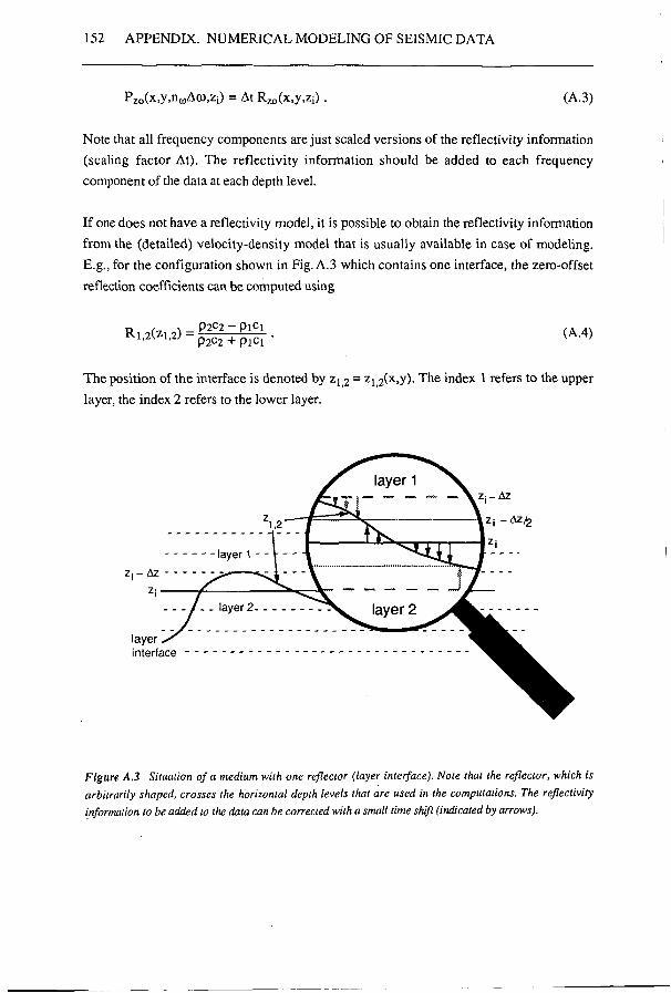
152 APPENDIX. NUMERICAL MODELING OF SEISMIC DATA
Pzo(x>y,no)Aa>,Zi) = At RZ0(x,y,Zi) . (A.3)
Note that all frequency components are just scaled versions of the reflectivity information (scaling factor At). The reflectivity information should be added to each frequency component of the data at each depth level.
If one does not have a reflectivity model, it is possible to obtain the reflectivity information from the (detailed) velocity-density model that is usually available in case of modeling. E.g., for the configuration shown in Fig. A.3 which contains one interface, the zero-offset reflection coefficients can be computed using
Rl,2(zi ,2) _ P2C2 - P1C1
P2C2 + P1C1 (A.4)
The position of the interface is denoted by z12 = Zii2(x,y). The index 1 refers to the upper layer, the index 2 refers to the lower layer.
layer interface
Figure A.3 Situation of a medium with one reflector (layer interface). Note that the reflector, which is arbitrarily shaped, crosses the horizontal depth levels that are used in the computations. The reflectivity information to be added to the data can be corrected with a small time shift (indicated by arrows).
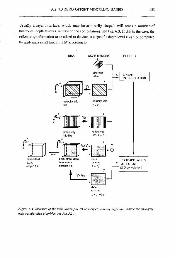
A.2 3D ZERO-OFFSET MODELING BASED 153
Usually a layer interface, which may be arbitrarily shaped, will cross a number of horizontal depth levels z; as used in the computations, see Fig. A.3. If this is the case, the reflectivity information to be added to the data at a specific depth level z, can be computed by applying a small time shift Ax according to
DISK CORE MEMORY k
PROCESS
f" 3 ^
LINEAR INTERPOLATION
velocity info file
velocity info
reflectivity info file
reflectivity info, z = z
CO ^
*"
S
s
t sort
Vz Ve *®
zero-offset data, output file
zero-offset data, temporary scratch file
data
L VzVa
EXTRAPOLATION Zj -»Z j -Az
(2-D convolution)
data
z = Z: -Az
Figure A.4 Structure of the table-driven full 3D zero-offset modeling algorithm. Notice the similarity
with the migration algorithm, see Fig. 5.2.1.
154 APPENDIX. NUMERICAL MODELING OF SEISMIC DATA
PzoCx.y^Aco.z;) = At RZ0(x,y,Zi) = At Ri,2(zi,2) e^"-*"** , (A.5)
for | zi,2 — z; | < Az/2.
The time shift is given by
A Z l , 2 - Z i
Ax = — . c
In Fig. A.4 a detailed scheme of the implementation of the the modeling program is shown. Note that this figure is very similar to Fig. 5.2.1 that shows the implementation of the migration.
The table-driven modeling technique discussed in this section was used to generate the synthetic 3D zero-offset data shown in Fig. 6.3.2 and 6.3.5.
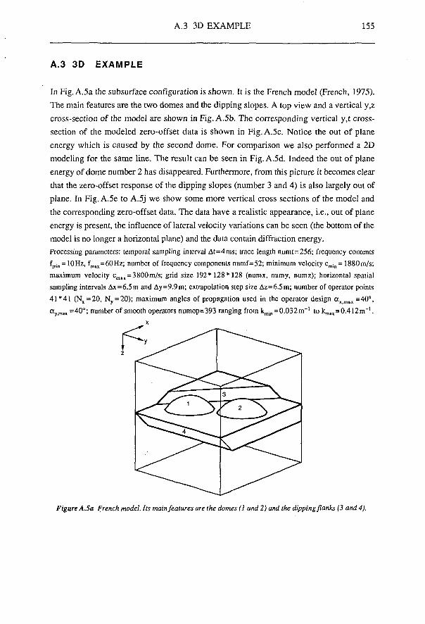
A.3 3D EXAMPLE 155
A.3 3D EXAMPLE
In Fig. A.5a the subsurface configuration is shown. It is the French model (French, 1975). The main features are the two domes and the dipping slopes. A top view and a vertical y,z cross-section of the model are shown in Fig. A.5b. The corresponding vertical y,t cross-section of the modeled zero-offset data is shown in Fig. A.5c. Notice the out of plane energy which is caused by the second dome. For comparison we also performed a 2D modeling for the same line. The result can be seen in Fig. A.5d. Indeed the out of plane energy of dome number 2 has disappeared. Furthermore, from this picture it becomes clear that the zero-offset response of the dipping slopes (number 3 and 4) is also largely out of plane. In Fig. A.5e to A.5j we show some more vertical cross sections of the model and the corresponding zero-offset data. The data have a realistic appearance, i.e., out of plane energy is present, the influence of lateral velocity variations can be seen (the bottom of the model is no longer a horizontal plane) and the data contain diffraction energy. Processing parameters: temporal sampling interval At=4ms; trace length numt=256; frequency contents fmin = 10Hz, fmilK=60Hz; number of frequency components numf=52; minimum velocity cmin = 1880m/s; maximum velocity cmai = 3800m/s; grid size 192*128*128 (numx, numy, numz); horizontal spatial sampling intervals Ax=6.5m and Ay=9.9m; extrapolation step size Az=6.5m; number of operator points 41*41 (1^ = 20, Ny = 20); maximum angles of propagation used in the operator design o l m a l =40°, ay.max =40°; number of smooth operators numop=393 ranging from kmin = 0.032nT1 to 1^,, = 0.412m"1.
Figure A.Sa French model. Its main features are the domes (1 and 2) and the dipping flanks (3 and 4).
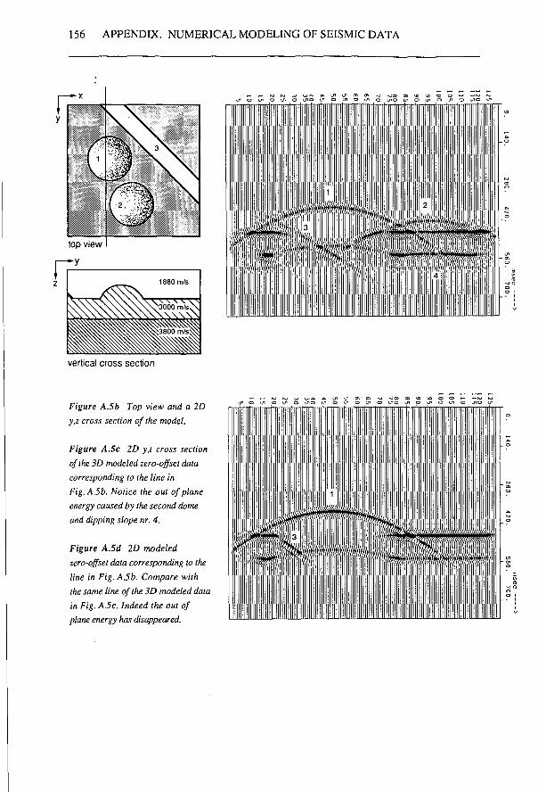
156 APPENDDC NUMERICAL MODELING OF SEISMIC DATA
vertical cross section
Figure A.5b Top view and a 2D y,z cross section of the model.
Figure A.Sc 2D y,t cross section of the 3D modeled zero-offset data corresponding to the line in Fig.A.5b. Notice the out of plane energy caused by the second dome and dipping slope nr. 4.
Figure A.5d 2D modeled zero-offset data corresponding to the line in Fig. A.5b. Compare with the same line of the 3D modeled data in Fig. A.5c. Indeed the out of plane energy has disappeared.
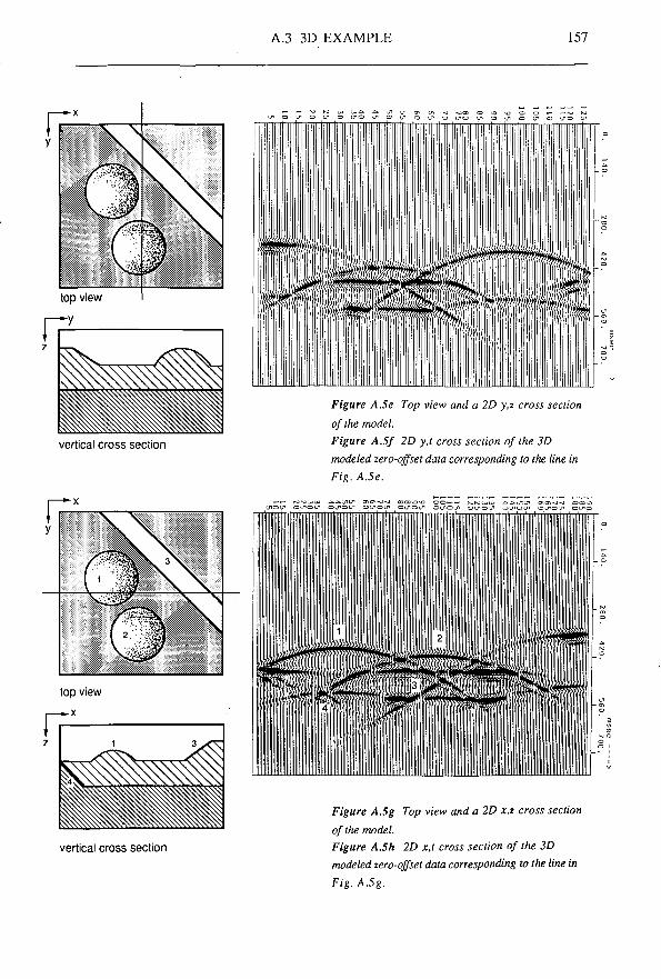
A.3 3D EXAMPLE 157
vertical cross section
Figure A.5e Top view and a 2D y,z cross section of the model. Figure A.5f 2D y,t cross section of the 3D modeled zero-offset data corresponding to the line in Fig. A.5e.
vertical cross section
Figure A.5g Top view and a 2D x,z cross section of the model. Figure A.Sh 2D x,t cross section of the 3D modeled zero-offset data corresponding to the line in Fig. A.5g.
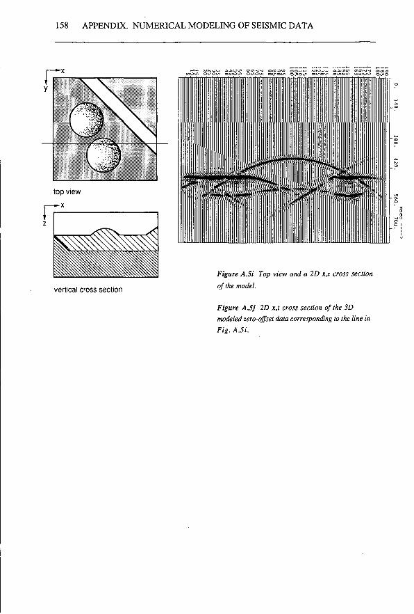
158 APPENDIX. NUMERICAL MODELING OF SEISMIC DATA
vertical crass section
Figure A.5i Top view and a 2D x,z cross section of the model.
Figure A.Sj 2D x,t cross section of the 3D modeled zero-offset data corresponding to the line in Fig. A.5i.
159
REFERENCES Baysal, E., Kosloff, D.D., and Sherwood, J.W.C., 1983,
Reverse time migration: Geophysics, v. 48, p. 1514 - 1524.
Berkhout, A. J., and Van Wulfften Palthe, D.W., 1979, Migration in terms of spatial deconvolution: Geophysical Prospecting, v. 27, p. 261 - 291.
Berkhout, A. J., 1985, Seismic migration; A. Theoretical aspects (3rd edition): Elsevier Scientific Publishing Company, Amsterdam.
Berkhout, A.J., 1984, Seismic migration; B. Practical aspects: Elsevier Scientific Publishing Company, Amsterdam.
Berkhout, A.J., 1984, Seismic resolution: Geophysical Press, Amsterdam.
Berkhout, AJ., Wapenaar, C.P.A., Blacquiere, G., and Kinneging, N.A., 1985, TRITON a three-year research proposal on Three-Dimensional Target Oriented Migration, Laboratory of Seismics and Acoustics, Delft University of Technology.
Berkhout, A.J., and Wapenaar, C.P.A., 1988, DELPHI a three-year research proposal on processing of elastic seismic data, Laboratory of Seismics and Acoustics, Delft University of Technology.
Brown, D. L., 1983, Applications of operator separation in reflection seismology: Geophysics, v. 48, p. 288 - 294.
Chang, W., and McMechan, G.A., 1989, 3-D Acoustic reverse-time migrations: Geophysical Prospecting, v 37, p. 243 - 256.
160 REFERENCES
Claerbout, J. F., 1970, !" Coarse grid calculations of waves in inhomogeneous media with application to delineation of complicated seismic structure: Geophysics, v. 35, p. 407 - 418.
Claerbout, J.F., 1985 (first published 1976), Fundamentals of geophysical data processing: Blackwell Scientific Publications, Oxford, UK.
Claerbout, J.F., 1985, Imaging the Earth's interior: Blackwell Scientific Publications Ltd., Oxford, UK.
Cox, H.L.H., Ooms, F.P.J., Wapenaar, C.P.A. and Berkhout, A.J., 1988, Verification of macro subsurface models using a shot record approach, 58th SEG meeting, Anaheim, Expanded abstracts, p. 904 - 908.
Debeye, H.W.J., 1988, Optimization of the recursive Kirchhoff extrapolator, I2-thesis, Delft University of Technology.
French, W.S., 1975, Computer migration of oblique seismic reflection profiles: Geophysics, v. 40, p. 961 - 980.
French, W.S., 1986, Trends in seismic data processing: Geophysics: the leading edge of exploration.
Gazdag, J., 1978, Wave-equation migration by phase shift: Geophysics, v. 43, p. 1342 - 1351.
Gazdag, J., 1981, Modeling of the acoustic wave equation with transform methods: Geophysics, v. 46, p. 854 - 859.
Gazdag, J., and Squazzero, P., 1984, Migration of seismic data by phase shift plus interpolation: Geophysics, v. 49, p. 124 - 131.
REFERENCES 161
Gibson, B., Lamer, K., and Levin, S., 1983, Efficient 3-D migration in two steps: Geophysical Prospecting, v. 31, p. 1 - 33.
Gill, P.E., Murray, W., and Wright, M., 1981, . Practical Optimization: Academic Press, London..
Hagedoorn, J.G., 1954, A process of seismic reflection interpretation: Geophysical Prospecting, v. 2, p. 85 - 127-
Holberg, O., 1988, Towards optimum one-way wave propagation: Geophysical Prospecting, v. 36, p. 99 - 114.
Hubral, P., 1977, Time migration - some ray theoretical aspects: Geophysical Prospecting, v. 25, p. 738 - 745.
Jakubowicz, H., and Levin, S., 1983, A simple exact method of 3-D migration - theory: Geophysical Prospecting, v. 31, p. 34 - 56.
Kinneging, N.A., 1989, Three-dimensional redatuming of seismic shot records, Thesis, Delft University of Technology.
Loewenthal, D., Lu, L., Roberson, R., and Sherwood, J.W.C., 1976, The wave equation applied to migration: Geophysics, v. 24, p. 380 - 399.
Loewenthal, D., Stoffa, P.L., and Faria, E.L., 1987, Suppressing the unwanted reflections of the full wave equation: Geophysical Prospecting, v. 52, p. 1007 - 1012.
McMechan, G.A., 1983, Migration by extrapolation of time-dependent boundary values: Geophysical Prospecting, v. 31, p. 413 - 420.
162 REFERENCES
Peels, G.L., 1988, True amplitude wave field extrapolation with application in seismic shot record redatuming, Thesis, Delft University of Technology.
Ristow, D., 1980, 3D-Downward extrapolation of seismic data in particular by finite difference methods, Thesis, Delft University of Technology.
Schneider, W. A., 1978, Integral formulation for migration in two and three dimensions: Geophysics, v. 43, p. 49 - 76.
Stolt, R.H., 1978, Migration by Fourier transform: Geophysics, v. 43, p. 2 3 - 4 8 .
Van der Made, P.M., 1988, Determination of macro subsurface models by generalized inversion, Thesis, Delft University of Technology.
Van der Schoot, A., 1989, Common reflection point stacking, Thesis, Delft University of Technology.
Verschuur, D.J., Herrmann, P., Kinneging, N.A., Wapenaar, C.P.A., and Berkhout, A.J., 1988, Elimination of surface-related multiply reflected and converted waves, 58th SEG meeting, Anaheim, Expanded abstracts, p. 1017 - 1020.
Wapenaar, C.P.A., 1986, Pre-stack migration in two and three dimensions, Thesis, Delft University of Technology.
Yilmaz, O., and Claerbout, J.F., 1980, Prestack partial migration: Geophysics, v. 45, p. 1753 - 1777.
163
SUMMARY
Chapter 1. To obtain an image of the subsurface of the Earth, seismic measurements are carried out. Elastic waves are transmitted into the subsurface and the reflected waves are detected at the surface and registered as a function of travel time. However, for a map of the subsurface the results should be presented as a function of depth instead of travel time. This transformation can be realized with seismic migration. A migration procedure requires a macro subsurface model to be present. Such a model of the subsurface defines the propagation properties (trend information on velocity and density). The determination of such a model is not a topic of this thesis: we consider the macro model as known. This thesis addresses the migration process itself. The seismic measurements are repeated at different surface locations and the results can be combined ('stacked'). The migration can be performed either before or after stacking. The results of prestack migration are better than those of poststack migration. However, prestack migration is not (yet) feasible for application in three dimensions because of the enormous computational cost. The TRITON*) approach offers a compromise: prestack 'redatuming' is carried out first. After this process the data can be considered as having been acquired at some level deep in the subsurface, e.g., at the upper boundary of the target zone. Next, common depth point (CDP) stacking is performed followed by full 3D zero-offset migration. The result is a depth image of the target. In Chapter 2 an inventory of wave field extrapolation techniques that are used in migration is given. The methods are classified according to the extrapolation coordinate (depth, time or vertical time), the application domain (space-time, space-frequency or wavenumber-frequency), the type of wave equation (one-way or two-way), the type of extrapolation (recursive or non-recursive) etc. For migration a choice is made for one-way, recursive extrapolation along the depth coordinate to be carried out in the space-frequency domain. Extrapolation is performed by using recursive Kirchhoff wave field extrapolation operators. The design of these operators is discussed in Chapter 3. Special attention is paid to aspects concerning aliasing, efficiency and accuracy. For use in practice two types of operators are presented: smooth operators and optimum operators. In the design of the smooth operator large spectral derivatives are avoided. The optimum operator is computed
TRITON represents an international consortium on migration research, carried out at the Laboratory of Seismics and Acoustics at the Delft University of Technology.
164 SUMMARY
by a least-squares algorithm. Smooth operators can be computed significantly faster than optimum operators. However, the latter ones can be applied more efficiently because they have the smallest possible size given a user-specified accuracy and dip range. The optimum operators are therefore suited for processing jobs with 'standard' acquisition parameters. Special sets of optimum operators could be generated for multiple use in those regular cases. Otherwise the smooth operators should be used. In either case the operators are stored in a table. This has the advantage that the operators do not need to be computed (more than once) during the actual extrapolation. In Chapter 4 the application of the operators in various migration techniques is discussed: from multi-offset via common-offset to zero-offset migration. For the 3D case zero-offset (poststack) depth migration is of most importance. Therefore, in Chapter 5 a detailed description of 3D table-driven zero-offset migration is given. Special attention is paid to the efficiency. The use of operators that have been computed in advance and stored in a table contributes considerably to a high efficiency. Furthermore, the symmetry properties of the operators are exploited which reduces the computational costs. We have formulated wave field extrapolation in terms of vector operations which makes the method very well suited for a vector computer. In addition a parallel implementation could be realized in a natural way because the frequency components are treated independently. Working per frequency component also has the advantage that the requirements concerning the computer memory remain moderate. Furthermore, in this chapter benchmark results are presented. From a cost comparison with reverse-time migration it follows that our table-driven migration is more efficient, not only with respect to the number of floating point operations (factor 10) but especially with respect to the required computer memory space (factor 103). In Chapter 6 2D and 3D examples of zero-offset migration are shown. All examples clearly show the excellent quality of our algorithm. The method can handle complex subsurface situations with both lateral and vertical velocity variations. Reflectors may be steeply dipping. After migration all events are positioned well and diffraction energy is focussed correctly. Furthermore, it is demonstrated that the results of full 3D migration are superior to those of the so-called 2 times 2D migration. Finally, in the Appendix the use of smooth operators or optimum operators in the modeling of 3D zero-offset data is discussed. This way of modeling yields better results than ray-tracing while it is significantly more efficient than finite-difference modeling.
165
SAMENVATTING
Hoofdstuk 1. Om een beeld te verkrijgen van de ondergrond van de aarde worden seismische metingen verricht. Elastische golven worden opgewekt in de aardbodem en de gereflecteerde golven worden aan de oppervlakte gedetecteerd en geregistreerd als functie van de looptijd. Op een kaart van de ondergrond moet het resultaat echter gepresenteerd worden als functie van de diepte in plaats van de looptijd. Het proces dat deze transformatie uitvoert heet seismische migratie. Een migratiemethode vereist dat een macro-model van de ondergrond aanwezig is. Een dergelijk model bevat de propagatie-eigenschappen (globale informatie betreffende de snelheid en de dichtheid) van de ondergrond. Het bepalen van het macromodel valt buiten het onderwerp van dit proefschrift: we beschouwen het macro-model als zijnde bekend en richten ons op het migratieproces zelf. De seismische metingen worden op verscheidene plaatsen aan de oppervlakte herhaald en de resultaten kunnen worden gecombineerd (Eng.: 'stacked'). De migratie kan zowel voor als na de stacking worden uitgevoerd. De resultaten van prestack migratie zijn beter dan die van poststack migratie. Voor toepassing in het geval van drie dimensionale data is prestack migratie (nog) niet mogelijk vanwege de enorm lange computer-rekentijden. De TRITON*) benadering biedt het volgende compromis. De eerste stap is prestack 'redatuming'. De resultaten hiervan kunnen worden opgevat alsof de seismische metingen uitgevoerd waren op een niveau diep in de ondergrond, bijvoorbeeld op de toplaag van het interessegebied. Vervolgens wordt een 'common depth point' (CDP) stacking uitgevoerd gevolgd door een volledig driedimensionale zero-offset migratie. Het resultaat is een afbeelding van het interessegebied als functie van de diepte. In Hoofdstuk 2 wordt een overzicht gegeven van de technieken voor golfveld-extrapolatie die gebruikt worden in migratie. De methoden zijn ingedeeld naar de extrapolatie-coördinaat (diepte, tijd of 'verticale tijd'), het toepassingsdomein (ruimte-tijd, ruimte-frequentie of golf getal-frequentie), het type golfvergelijking (eenweg of tweeweg), het type extrapolatie (recursief of niet-recursief) enz. De keuze voor migratie is: eenweg recursieve extrapolatie langs de dieptecoordinaat in het ruimte-frequentie domein.
TRITON is een internationaal door de industrie gesponsord project. Het onderzoek is op het gebied van migratie en wordt uitgevoerd bij de Vakgroep Seismiek en Akoestiek, Technische Universiteit Delft.
166 SAMENVATTING
Extrapolatie wordt uitgevoerd met gebruikmaking van recursieve Kirchhoff operatoren voor golfveld-extrapolatie. Bij het ontwerp van deze operatoren, die besproken worden in Hoofdstuk 3, wordt speciale aandacht besteed aan aspecten betreffende aliasing, efficiëntie en nauwkeurigheid. Voor het gebruik in de praktijk worden twee typen operatoren voorgesteld: geëffende operatoren en optimale operatoren. Bij het berekenen van de geëffende operator worden grote spectrale afgeleiden vermeden. De optimale operator wordt bepaald met behulp van een kleinste-kwadraten algoritme. Geëffende operatoren kunnen beduidend sneller berekend worden dan optimale operatoren. De laatste zijn echter efficiënter in hun toepassing omdat zij de kleinst mogelijke afmeting hebben, gegeven de specificaties van de gebruiker omtrent nauwkeurigheid en hoekbereik. Om die reden zijn optimale operatoren het meest geschikt voor toepassing in gevallen met 'standaard' acquisitie parameters. Voor die gevallen zouden speciale sets van optimale operatoren gemaakt kunnen worden om telkens opnieuw te gebruiken. In de overige situaties kunnen dan de geëffende operatoren gebruikt worden. Voor beide operatortypen geldt dat de operatoren voor gebruik worden opgeslagen in een tabel. Dit voorkomt (meervoudige) berekening van de operatoren tijdens de feitelijke extrapolatie. In Hoofdstuk 4 wordt de toepassing van de operatoren in diverse migratietechnieken besproken: van multi-offset via common-offset naar zero-offset migratie. Voor de 3D situatie is zero-offset (poststack) migratie het meest belangrijk. Daarom volgt in Hoofdstuk 5 een gedetailleerde beschrijving van 3D tabel-gedreven zerooffset migratie. Speciale aandacht wordt besteed aan de efficiëntie. Het gebruik van vooraf berekende operatoren die vervolgens opgeslagen worden in een tabel leidt tot een aanzienlijke verhoging van de efficiëntie. Ook de symmetrie-eigenschappen van de operatoren worden benut om de rekentijden te bekorten. We hebben golfveld-extrapolatie geformuleerd in termen van vectorbewerkingen. Dit maakt de methode bijzonder geschikt voor vectorcomputers. Bovendien kan een implementatie voor een parallelle machine op een natuurlijke manier gerealiseerd worden omdat de frequentiecomponenten onafhankelijk worden verwerkt. Het uitvoeren van de berekeningen per frequentiecomponent heeft verder het voordeel dat het benodigde computergeheugen bescheiden kan blijven. In dit hoofdstuk worden de resultaten van een benchmark gepresenteerd. Uit een kostenvergelijking met 'reverse-time' migratie blijkt dat onze tabel-gedreven migratie veel efficiënter is. Dit geldt niet alleen voor het aantal rekenkundige bewerkingen (factor 10) maar speciaal ook voor het vereiste computergeheugen (factor 103). In Hoofdstuk 6 worden 2D en 3D voorbeelden van zero-offset migratie getoond. Alle
SAMENVATTING 167
voorbeelden laten duidelijk de goede kwaliteit van het algoritme zien. De methode kan complexe ondergrond-situaties aan waarin zowel laterale als verticale snelheidsvariaties optreden. Reflectoren mogen steil zijn. In de resultaten van de migratie is de positionering in orde; ook is diffractie energie goed gefocusseerd. Verder wordt aangetoond dat de resultaten van 3D migratie beter zijn dan die van de zgn. 2 maal 2D migratie. Tenslotte wordt in de Appendix de toepassing van geëffende operatoren of optimale operatoren in het modelleren van 3D zero-offset data besproken. Deze manier van modelleren levert betere resultaten dan 'ray-tracing' terwijl zij beduidend efficiënter is dan 'finite-difference' modelleren.
168
CURRICULUM VITAE
Blacquière, Gerrit 17 maart 1960 Zwijndrecht
Lager onderwijs te Aerdenhout Middelbaar onderwijs (Gymnasium 6) te Haarlem Technische Hogeschool Delft Technische Natuurkunde 1983: Kandidaats examen 1985: Doctoraalexamen
4e-jaars onderzoek: Stable finite-difference wave field extrapolation. afstudeeronderzoek: 3D Seismic migration for the case of horizontally layered media.
WERKERVARING 1985 - 1989 Wetenschappelijk onderzoeker aan de Technische
Universiteit Delft, Vakgroep Akoestiek en Seismiek, bij het TRITON project en het DELPHI project.
Naam Geboortedatum Geboorteplaats
OPLEIDING 1966-1972 1972-1978 1978-1985