Seismic Velocity Estimation from Time Migration

M. K. Cameron, S. B. Fomel, J. A. Sethian ∗

April 23, 2007

Abstract

We address the problem of estimating seismic velocities inside the earth which is necessaryfor obtaining seismic images in regular Cartesian coordinates. The main goals are to developalgorithms to convert time-migration velocities to true seismic velocities, and to convert time-migrated images to depth images in regular Cartesian coordinates.

Our main results are three-fold. First, we establish a theoretical relation between the trueseismic velocities and the ”time migration velocities” using the paraxial ray tracing. Second,we formulate an appropriate inverse problem describing the relation between time migrationvelocities and depth velocities, and show that this problem is mathematically ill-posed, i.e.,unstable to small perturbations.

Third, we develop numerical algorithms to solve regularized versions of these equations whichcan be used to recover smoothed velocity variations. Our algorithms consist of efficient time-to-depth conversion algorithms, based on Dijkstra-like Fast Marching Methods, as well as level setand ray tracing algorithms for transforming Dix velocities into seismic velocities. Our algorithmsare applied to both two-dimensional and three-dimensional problems, and we test them on acollection of both synthetic examples and field data.

1 Introduction

Seismic data are the records of the sound wave amplitudes P described by the wave equation

∆P (x, y, z; t) =1

v2(x, y, z)∂2

∂t2P (x, y, z; t). (1)

where v(x, y, z) is speed of propagation of the waves in the earth. In this work, we consider onlythe seismic data coming from the acoustic P waves and refer to v(x, y, z) as the seismic velocity.This velocity is typically unknown, and its determination is the subject of the present work.

One common fast and robust process of obtaining seismic images is called time migration (seee.g. [Yilmaz, 2001]). This process is considered adequate for the areas with mild lateral velocityvariation, i.e. where v depends mostly on z and only slightly on x and y. However, even mildlateral velocity variations can significantly distort subsurface structures on the time migratedimages. Moreover, time migration produces images in very specific time migration coordinates

∗This work was supported in part by the Applied Mathematical Science subprogram of the Office of EnergyResearch, U.S. Department of Energy, under Contract Number DE-AC03-76SF00098, and by the ComputationalMathematics Program of the National Science Foundation

1

(x0, t0) (explained below), and the relation between them and the Cartesian coordinates can benontrivial if the velocity varies laterally.

One “side product” of time migration is mean velocities vm(x0, t0), known as time migrationvelocities. We will refer to them as migration velocities for brevity. In the case where the seismicvelocity depends only on the depth, these velocities are close to the root-mean-square (RMS)velocities [Dix, 1955]. In the general case, these velocities relate to the radius of curvature ofthe emerging wave front [Hubral and Krey, 1980].

An alternative approach to obtaining seismic images is called depth migration [Yilmaz, 2001].This approach is adequate for areas with lateral velocity variation, and produces seismic imagesin regular Cartesian depth coordinates, which are commonly called depth coordinates. Themajor problem with this approach is that its implementation requires the construction of avelocity model for the seismic velocity v(x, y, z). It can be both difficult and time consuming toconstruct an adequate velocity model: an iterative approach of guesswork followed by correctionis often employed.

The main idea of this work is to construct a velocity model v(x) from the migration velocitiesgiven in the time migration coordinates (x0, t0) (see a block-scheme in Fig. 1). Using thesevelocities one can then perform depth migration to obtain an improved seismic image in theCartesian coordinates x. As an alternative to depth migration, one can instead directly converta time migrated image to ”depth” (regular Cartesian coordinates) using the additional outputsof our construction x0(x) and t0(x).

Figure 1: The main idea of this work.

Thus, our goals are to create fast and robust algorithms to:

1. Convert the migration velocities vm(x0, t0) to the true seismic velocities v(x);

2. Convert time migrated images (in (x0, t0) coordinates) to ”depth” (to images in regularCartesian coordinates x).

The end result is to construct more accurate seismic images cheaply and routinely. Our resultsare the following:

1. We begin by producing theoretical relations between the migration velocity and the trueseismic velocity in 2D and 3D.

• In 2D the Dix velocities vDix(x0, t0) which are a conventional estimate of true seismicvelocities from the migration velocities, can be used instead of the migration velocitiesas a more convenient input.

2

• The input data in the 3D case are a bit different. Time migration can be performedin such a way that a set of certain 2 × 2 matrices K(x0, y0, t0) is determined. Thesematrices divided by the time t0 have dimension of the velocity squared, and we cancall the entry-wise square roots of them migration velocities. They can be easilyconverted into matrices F(x0, y0, t0) which we use as an input for our 3D numerics.

2. Next, we formulate an appropriate inverse problem describing the relation between timemigration velocities and seismic velocities, and show that this problem is mathematicallyill-posed, i.e., unstable to small perturbations.

3. We develop numerical algorithms to solve the regularized versions of this problem in 2D and3D which can be used to recover smoothed velocity variations. Our algorithms consist ofefficient time-to-depth conversion algorithms, based on Dijkstra-like Fast Marching Meth-ods, as well as level set and ray tracing algorithms. The relation between the approachesand the algorithms in 2D and 3D are outlined in Fig. 2 (a) and (b) respectively.

4. Finally, we test our algorithms in 2D and 3D on a collection of examples.

(a) (b)

Figure 2: The approaches and the algorithms: (a) 2D, (b) 3D.

1.1 Time migration coordinates and image rays

Seismic migration is an operation that moves recorded reflection events to the origin of reflec-tion. The most efficient kind of migration is time migration based on an approximation of thetraveltime. Hubral (1977) introduced the concept of the image ray, which gives the connectionbetween the time migration coordinates and the regular Cartesian coordinates.

To explain this idea, we begin with the high frequency approximation applied to the waveequation (1), in which the wave front T (x, y, z) propagates according to the Eikonal equation(see e.g. [Popov, 2002]):

|∇T (x, y, z)|2 =1

v2(x, y, z). (2)

The characteristics of the Eikonal equation can be viewed as rays. Among all rays startingat a subsurface point R and reaching earth’s surface (Fig. 3), some have minimal travel time.These rays are called image rays, and it is easy to see that they must arrive perpendicular tothe surface. The ray RI in Fig. 3 is one such image ray. Thus, we may characterize the pointR in one of two coordinate systems: either (1) its natural Cartesian coordinates x or (2) the

3

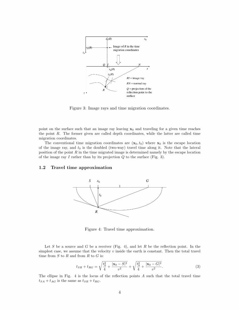
Figure 3: Image rays and time migration coordinates.

point on the surface such that an image ray leaving x0 and traveling for a given time reachesthe point R. The former given are called depth coordinates, while the latter are called timemigration coordinates.

The conventional time migration coordinates are (x0, t0) where x0 is the escape locationof the image ray, and t0 is the doubled (two-way) travel time along it. Note that the lateralposition of the point R in the time migrated image is determined namely by the escape locationof the image ray I rather than by its projection Q to the surface (Fig. 3).

1.2 Travel time approximation

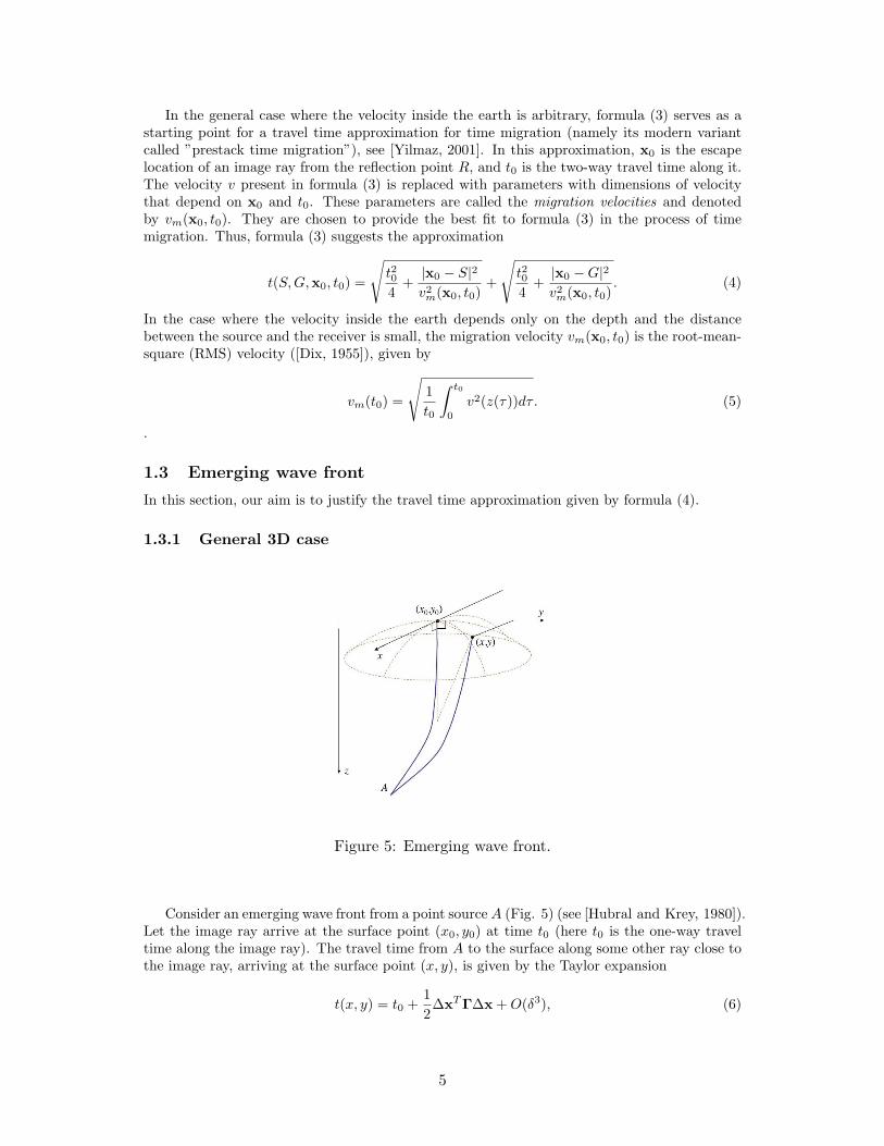
Figure 4: Travel time approximation.

Let S be a source and G be a receiver (Fig. 4), and let R be the reflection point. In thesimplest case, we assume that the velocity v inside the earth is constant. Then the total traveltime from S to R and from R to G is:

tSR + tRG =

√t204

+|x0 − S|2

v2+

√t204

+|x0 −G|2

v2. (3)

The ellipse in Fig. 4 is the locus of the reflection points A such that the total travel timetSA + tAG is the same as tSR + tRG.

4

In the general case where the velocity inside the earth is arbitrary, formula (3) serves as astarting point for a travel time approximation for time migration (namely its modern variantcalled ”prestack time migration”), see [Yilmaz, 2001]. In this approximation, x0 is the escapelocation of an image ray from the reflection point R, and t0 is the two-way travel time along it.The velocity v present in formula (3) is replaced with parameters with dimensions of velocitythat depend on x0 and t0. These parameters are called the migration velocities and denotedby vm(x0, t0). They are chosen to provide the best fit to formula (3) in the process of timemigration. Thus, formula (3) suggests the approximation

t(S,G,x0, t0) =

√t204

+|x0 − S|2v2m(x0, t0)

+

√t204

+|x0 −G|2v2m(x0, t0)

. (4)

In the case where the velocity inside the earth depends only on the depth and the distancebetween the source and the receiver is small, the migration velocity vm(x0, t0) is the root-mean-square (RMS) velocity ([Dix, 1955]), given by

vm(t0) =

√1t0

∫ t0

0

v2(z(τ))dτ. (5)

.

1.3 Emerging wave front

In this section, our aim is to justify the travel time approximation given by formula (4).

1.3.1 General 3D case

Figure 5: Emerging wave front.

Consider an emerging wave front from a point sourceA (Fig. 5) (see [Hubral and Krey, 1980]).Let the image ray arrive at the surface point (x0, y0) at time t0 (here t0 is the one-way traveltime along the image ray). The travel time from A to the surface along some other ray close tothe image ray, arriving at the surface point (x, y), is given by the Taylor expansion

t(x, y) = t0 +12

∆xTΓ∆x +O(δ3), (6)

5

where ∆x =(x− x0

y − y0

), Γ is the matrix of the second derivatives of t(x, y) evaluated at the

point (x0, y0) and δ =√

(x− x0)2 + (y − y0)2. From geometrical considerations, one can obtain(see [Hubral and Krey, 1980]) a relation between the matrix Γ and the matrix R of the radii ofcurvature of the emerging wave front, namely

Γ−1 = Rv(x0, y0), (7)

where v(x0, y0) = v(x = x0, y = y0, z = 0) is the velocity at the surface point (x0, y0). Forconvenience, we will work with the inverse of the matrix Γ which we denote by K:

K = Γ−1 = Rv(x0, y0). (8)

1.3.2 2D simplification

In the case where sources and receivers are arranged along some straight line, seismic imagingbecomes a 2D problem, and equation (6) can be simplified to

t(x) = t0 +12

(x− x0)2txx(x = x0) +O(δ3) = t0 +(x− x0)2

2Rv(x0)+O(δ3), (9)

where v(x0) ≡ v(x = x0, z = 0). By squaring both sides of equation (9) we get:

t2(x) = t20 + (x− x0)2t0txx(x = x0) +O(δ3) = t20 + (x− x0)2t0

Rv(x0)+O(δ3). (10)

Suppose we want to compute the total travel time from a source S to the reflection point A andfrom A to a receiver G. Using equation (10) we obtain:

t(x0, t0, S,G) = tSA + tAG =

√t20 + (S − x0)2

t0Rv(x0)

+

√t20 + (G− x0)2

t0Rv(x0)

+O(δ3). (11)

Comparing equations (11) and (4) we see that the travel time approximation given by formula(4) follows from the Taylor expansion in 2D. Moreover, the migration velocity and the radius ofcurvature of the emerging wave front are converted through the relation

t0v2m(x0, t0) = v(x0)R(x0, t0). (12)

On the other hand, in 3D the travel time approximation given by formula (4) is not asstraightforward. Instead, one can easily derive the following travel time formula from equations(6) and (7):

t(x0, t0, S,G) =√t20 + t0(S − x0)TK(x0, t0)−1(S − x0) (13)

+√t20 + t0(G− x0)TK(x0, t0)−1(G− x0).

However note that if the velocity depends only on the depth, the matrix K is a multiple ofthe identity matrix, and hence formula (4) is the consequence of the Taylor expansion.

1.4 Dix inversion

Dix ([Dix, 1955]) established the first connection between the migration velocities and the seis-mic velocities for the case where the velocity depends only on the depth. He showed that themigration velocities are the root-mean-square (RMS) velocities if the distances between thesources and the receivers are small and developed the following inversion method. Consider anearth model as in Fig. 6. Let the layers be flat and horizontal, and the velocity be constantwithin each layer. We are given the RMS velocities Vi and the travel times ti, i = 1, 2, ..., n,

6

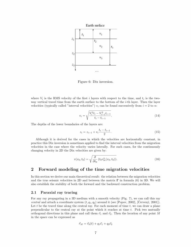
Figure 6: Dix inversion.

where Vi is the RMS velocity of the first i layers with respect to the time, and ti is the two-way vertical travel time from the earth surface to the bottom of the i-th layer. Then the layervelocities (typically called ”interval velocities”) vi can be found successively from i = 2 to n:

vi =

√V 2i ti − V 2

i−1ti−1

ti − ti−1. (14)

The depths of the lower boundaries of the layers are:

zi = zi−1 + viti − ti−1

2. (15)

Although it is derived for the cases in which the velocities are horizontally constant, inpractice this Dix inversion is sometimes applied to find the interval velocities from the migrationvelocities in the case where the velocity varies laterally. For such cases, for the continuouslychanging velocity in 2D the Dix velocities are given by:

v(x0, t0) =√

∂

∂t0(t0v2

m(x0, t0)). (16)

2 Forward modeling of the time migration velocities

In this section we derive our main theoretical result: the relation between the migration velocitiesand the true seismic velocities in 2D and between the matrix Γ in formula (6) in 3D. We willalso establish the stability of both the forward and the backward construction problem.

2.1 Paraxial ray tracing

For any ray propagating in a 3D medium with a smooth velocity (Fig. 7), we can call this raycentral and attach a coordinate system (t, q1, q2) around it (see [Popov, 2002], [Cerveny, 2001]).Let t be the travel time along the central ray. For each moment of time t, we can draw a planeperpendicular to the central ray at the point which it reaches at time t. Pick two mutuallyorthogonal directions in this plane and call them ~e1 and ~e2. Then the location of any point Min the space can be expressed as

~rM = ~r0(t) + q1~e1 + q2~e2

7

for some t, q1 and q2, where ~r0(t) gives the point reached by the central ray at time t. If M isclose enough to the ray, its location can be described by (t, q1, q2) uniquely.

Figure 7: Paraxial ray tracing.

Suppose that the central ray is surrounded by a family of close rays and we want to writeequations of those rays in terms of q1(t) and q2(t) (Fig. 7). In order to apply the Hamiltonianformalism, we need to introduce the generalized momentums p1 and p2 corresponding to thegeneralized coordinates q1 and q2. We first note the fact that the central ray is a ray itself, andthis imposes the following requirements on the evolution of ~e1 and ~e2:

d~e1dt

=∂v(t, q1, q2)

∂q1 q1=q2=0

~τ ,d~e2dt

=∂v(t, q1, q2)

∂q2 q1=q2=0

~τ ,

where ~τ is the unit tangent vector to the central ray ([Popov, 2002]). The ray equations in theHamiltonian form are ([Popov, 2002], [Popov and Psencik, 1978],[Cerveny, 2001]):

d

dt

(qp

)=(

0 v20I2

− 1v0

V 0

)(qp

). (17)

Here v0 is the velocity along the central ray, I2 is the 2 × 2 identity matrix, and V is a 2 × 2matrix of the second derivatives of the velocity:

Vij =∂2v(t, q1, q2)∂qi∂qj

, i, j = 1, 2.

Suppose that the family of rays depends upon two parameters (α1, α2). There are twoimportant cases (see Fig. 8):

• All rays start perpendicular to the same plane. Then (α1, α2) can be chosen to be theinitial coordinates (x0, y0) of the rays at this plane. We will call such a family of raystelescopic.

8

• All rays start at the same point, but in different directions. Then (α1, α2) can be chosento be the initial momentums (p1(0), p2(0)) of the rays. We will call such a family the pointsource family.

Consider the following 2× 2 matrices ([Popov, 2002], [Cerveny, 2001]):

Qij ≡∂qi∂αj

, Pij ≡∂pi∂αj

, i, j = 1, 2. (18)

The equations of time evolution for Q and P are the equations in variations for equation (17):

d

dt

(QP

)=(

0 v20I2

− 1v0

V 0

)(QP

). (19)

The initial conditions for the telescopic family of rays are

Q(0) = I2, P(0) = 0, (20)

and for the point source family they are

Q(0) = 0, P(0) =1

v0(0)I2, (21)

where v0(0) is the velocity at the source point. The absolute value of the determinant of thematrix Q has a nice geometrical sense ([Popov, 2002]):

|det Q| is the geometrical spreading of the family of rays.

Let the central ray arrive orthogonal to some plane at a point (x0, y0). Consider the matrixΓ of the second derivatives of the travel times of the family of rays around the central ray,evaluated at the point (x0, y0). E.g., the central ray can be the image ray arriving to the earthsurface. Then the matrix Γ is defined by formula 6) for the source point family of rays from thesource point A as in Fig. 5. In [Popov, 2002], [Cerveny, 2001] it was shown that

Γ = PQ−1 (22)

andd

dtΓ = −v2

0Γ2 − 1v0

V. (23)

For convenience, in the present work we will deal with the matrix K = Γ−1, which is the matrixof radii of curvature of the wave front scaled by the velocity at the image ray, namely

K = v0R = QP−1. (24)

One can easily derive from equation (23) that the time evolution of K is given by:

d

dtK = v2

0I2 +1v0

KVK. (25)

For the point source family of rays the initial conditions for the matrix K are:

K(0) = 0. (26)

2.2 Relation between the matrices K and the true seismic velocitiesin 3D

We have established the relation between the matrices K and the seismic velocities in 3Dformulated in Theorem 1 below. The matrix K in formula (13) is a matrix of parametersdepending on x0 and t0, which can be estimated from the measurements. Theorem 1 providesa connection between the matrix K and the true seismic velocity at the subsurface point xreached by the image ray arriving at x0 and traced backwards for time t0 (Fig. 8).

9

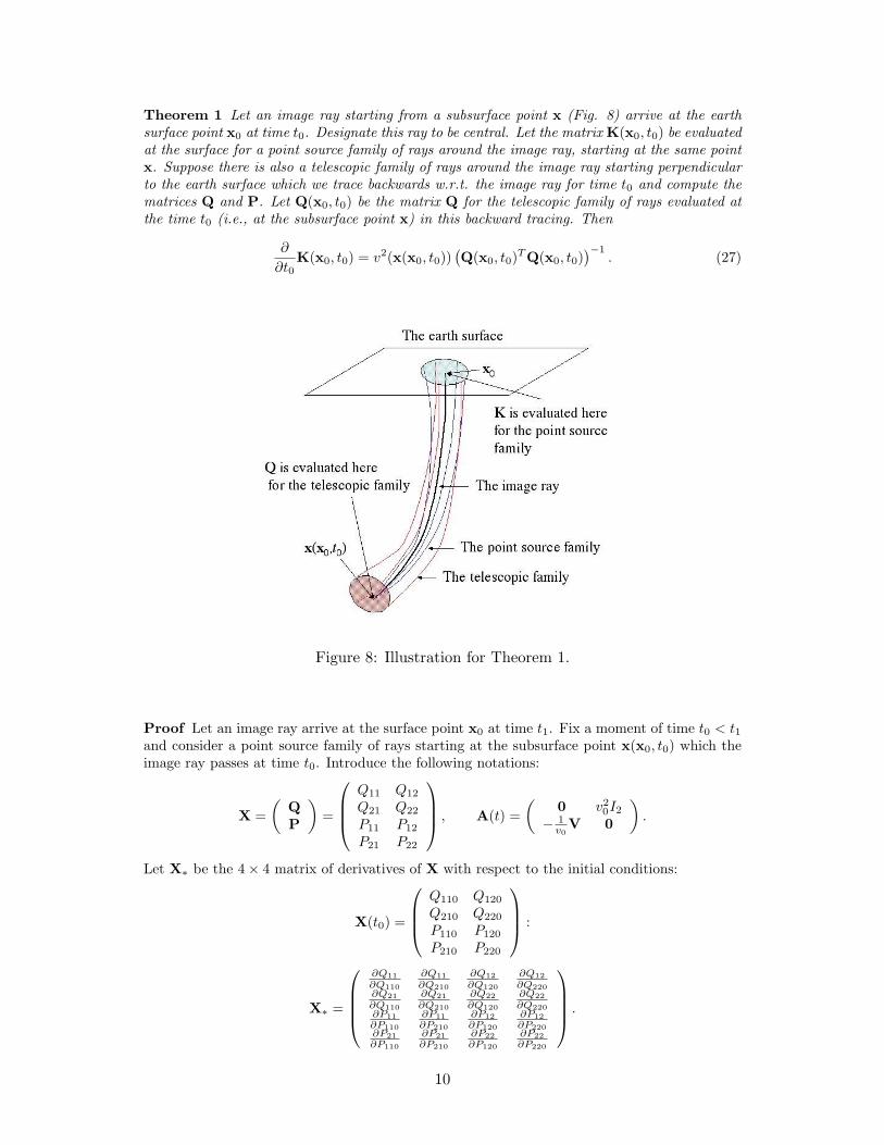
Theorem 1 Let an image ray starting from a subsurface point x (Fig. 8) arrive at the earthsurface point x0 at time t0. Designate this ray to be central. Let the matrix K(x0, t0) be evaluatedat the surface for a point source family of rays around the image ray, starting at the same pointx. Suppose there is also a telescopic family of rays around the image ray starting perpendicularto the earth surface which we trace backwards w.r.t. the image ray for time t0 and compute thematrices Q and P. Let Q(x0, t0) be the matrix Q for the telescopic family of rays evaluated atthe time t0 (i.e., at the subsurface point x) in this backward tracing. Then

∂

∂t0K(x0, t0) = v2(x(x0, t0))

(Q(x0, t0)TQ(x0, t0)

)−1. (27)

Figure 8: Illustration for Theorem 1.

Proof Let an image ray arrive at the surface point x0 at time t1. Fix a moment of time t0 < t1and consider a point source family of rays starting at the subsurface point x(x0, t0) which theimage ray passes at time t0. Introduce the following notations:

X =(

QP

)=

Q11 Q12

Q21 Q22

P11 P12

P21 P22

, A(t) =(

0 v20I2

− 1v0

V 0

).

Let X∗ be the 4× 4 matrix of derivatives of X with respect to the initial conditions:

X(t0) =

Q110 Q120

Q210 Q220

P110 P120

P210 P220

:

X∗ =

∂Q11∂Q110

∂Q11∂Q210

∂Q12∂Q120

∂Q12∂Q220

∂Q21∂Q110

∂Q21∂Q210

∂Q22∂Q120

∂Q22∂Q220

∂P11∂P110

∂P11∂P210

∂P12∂P120

∂P12∂P220

∂P21∂P110

∂P21∂P210

∂P22∂P120

∂P22∂P220

.

10

Note that since each of the columns of X is a linear independent solution of equation (17) thederivatives not included into X∗ are zeros. X(t) and X∗(t) are solutions of the following initialvalue problems:

dXdt

= A(t)X, X(t0) =1

v(t0)

(0I2

), (28)

where v(t0) = v(x(x0, t0)), and

dX∗dt

= A(t)X∗, X∗(t0) = I4. (29)

Denote the solution of equation (29) by B(t0; t1) as it is done in [Cerveny, 2001]:

B(t0; t1) =(

Q1 Q2

P1 P2

),

where Qi, Pi, i = 1, 2 are 2× 2 matrices.(

Q1

P1

)satisfies the initial conditions corresponding

to a telescopic point, and(

Q2

P2

)satisfies the initial conditions corresponding to a normalized

point source. B(t0, t1) is called the propagator matrix. Then the solution of (28) is:

X(t) =1

v(t0)

(Q2

P2

). (30)

Now turn to the matrix K: K(t0; t1) = Q(t0; t1)P(t0; t1)−1 = Q2P−12 .

Shift the initial time t0 by −∆t. Then, according to equation (28) at time t0

Q(t0 −∆t; t0) = 0 + ∆tv2(t0)1

v(t0)I2 +O((∆t)2),

P(t0 −∆t; t0) =1

v(t0)I2 +O((∆t)2).

Hence the change in the initial conditions for equation (28) is:

∆Q0 = v0∆tI2 +O((∆t)2), ∆P0 = 0 +O((∆t)2). (31)

Then

K(t0 −∆t; t1) = K(t0; t1) +2∑

i,j=1

∂K∂Qij0

∆Qij0 +2∑

i,j=1

∂K∂Pij0

∆Pij0 +O((∆t)2) (32)

= K(t0; t1) +(

∂K∂Q110

+∂K∂Q220

)v(t0)∆t+O((∆t)2).

Let us find the partial derivatives in the expression above:

∂K∂Qii0

=∂Q∂Qii0

P−1 −QP−1 ∂P∂Qii0

P−1, i = 1, 2. (33)

In terms of the entries of the matrix B(t0; t1)

∂K∂Q110

+∂K∂Q220

= v0(Q1P−12 −Q2P−1

2 P1P−12 ). (34)

In [Cerveny, 2001] the symplectic property of the matrix B(t0; t1) was proved:

BTJB = J, (35)

11

where J is the 4× 4 matrix

J =(

0 I2−I2 0

).

To simplify formula (34) we will use the following consequences of the symplectic property (35):

PT2 Q1 −QT

2 P1 = I2, PT2 Q2 = QT

2 P2. (36)

Then the matrix expression in equation (34) simplifies to:

Q1P−12 −Q2P−1

2 P1P−12 =

(PT2 )−1PT

2 Q1P−12 − (PT

2 )−1PT2 Q2P−1

2 P1P−12 =

(PT2 )−1(PT

2 Q1 −PT2 Q2P−1

2 P1)P−12 =

(PT2 )−1(PT

2 Q1 −QT2 P2P−1

2 P1)P−12 =

(PT2 )−1(PT

2 Q1 −QT2 P1)P−1

2 =

(PT2 )−1P−1

2 . (37)

Substituting Eqn. (37) to Eqn. (34) and then to Eqn. (32) we get:

K(t0 −∆t; t1) = K(t0; t1) + ∆tv2(t0)(PT2 )−1P−1

2 +O((∆t)2). (38)

Then the derivative of K with respect to the initial time is:

−∂K(t0; t1)∂t0

= v2(t0)(PT2 )−1P−1

2 . (39)

In [Cerveny, 2001] the following reciprocity property was proved:

PT2 (x1,x2) = Q1(x2,x1), (40)

where x1, x2 are the end points of the central ray. Applying it to equation (39) and taking thetime reverse into account we obtain formula (27).

2.3 Relation between the Dix velocities and the true seismic velocitiesin 2D

In 2D the matrices Q, P and K become scalars which we denote by Q, P and K respectively.K is the radius of curvature of the wave front scaled by the velocity at the central ray: K = vR.The time evolution of Q, P and K are given by:

d

dt

(QP

)=(

0 v20

−vqq

v00

)(QP

),

dK

dt= v2 +

vqqvK2. (41)

In a similar way as it was done in 3D, it can be proven that

∂

∂t0K(x0, t0) =

v2(x(x0, t0), z(x0, t0))Q2(x0, t0)

. (42)

Then taking into account the definition of the Dix velocity (16) and the relation (12) betweenthe migration velocities and the radius of curvature of the emerging wave front we have thefollowing:

Theorem 2 Let an image ray arrive to the earth surface point x0 at time t0 from a subsurfacepoint (x, z). Suppose there is a telescopic family of rays around the image ray starting per-pendicular to the earth surface which we trace backwards w.r.t. the image ray for time t0 andcompute the quantities Q and P . Let Q(x0, t0) be the quantity Q for the telescopic family of raysevaluated at the time t0 (i.e., at the subsurface point (x, z)) in this backward tracing. Then the

12

Dix velocity vDix(x0, t0) is the ratio of the true seismic velocity v(x, z) and the absolute valueof Q(x0, t0):

vDix(x0, t0) =v(x(x0, t0), z(x0, t0))

|Q(x0, t0)|. (43)

Note that here, t0 is the one-way travel time along the image ray and that we denote thedepth direction by z.

3 Stability of the forward and backward (inverse) con-struction problem

We state an inverse problem both in 2D and in 3D. Here, t0 will denote the one-way travel timealong the image ray.

3.1 The inverse problem in 2D

Suppose there is an image ray arriving at each surface point x0, xmin ≤ x0 ≤ xmax. For any0 ≤ t0 ≤ tmax, trace the image ray backward for time t0 together with a small telescopic family ofrays. Let the image ray being traced backward reach a subsurface point (x, z) at time t0. Denoteby v(x0, t0) the velocity at the point (x, z), and by Q(x0, t0) the quantity Q for the correspondingtelescopic family at the point (x, z). We are given vDix(x0, t0) = v(x(x0,t0),z(x0,t0))

|Q(x0,t0)| ≡ f(x0, t0),xmin ≤ x0 ≤ xmax, 0 ≤ t0 ≤ tmax. We need to find v(x, z), the velocity inside the domaincovered with the image rays arriving to the surface in the interval [xmin, xmax].

The first question is whether this problem is well-posed. In the next sections, we will showthat both the direct problem (given v(x, z) find f(x0, t0)) and the inverse problem (given f(x0, t0)find v(x, z)) are ill-posed. We will use the notation f(x0, t0) ≡ v(x(x0,t0),z(x0,t0))

|Q(x0,t0)| rather thanvDix(x0, t0) to emphasize that f is computed as the ratio v/|Q| rather than from the optimalmigration velocities.

3.1.1 Ill-posedness of the direct problem

Direct Problem: Given v(x, z), xmin ≤ x ≤ xmax, xmin < 0, xmax > 0, z ≥ 0 and tmax findf(x0, t0) = v(x0,t0)

|Q(x0,t0)| , xmin ≤ x0 ≤ xmax, 0 ≤ t0 ≤ tmax.

We shall show that small changes in v(x, z) can lead to large changes in f(x0, t0). Takev(x, z) = 1 and v(x, z) = 1 + a cos(kx), −1 ≤ x ≤ 1. Then

||v − v||∞ = a.

Obviously, f(x0, t0) = 1 for v(x, z) = 1. Compute f(x0, t0) for v(x, z) at x0 = 0. As the imageray arriving at x0 = 0 is straight, we have that

vqq = vxx(x = 0) = −ak2.

Then we have:

dQ

dt0= (1 + a2)P,

dP

dt0=

ak2

1 + aQ, Q(0) = 1, P (0) = 0.

Therefore,d2Q

dt20=ak2(1 + a2)

1 + aQ, Q(0) = 1,

dQ

dt0= 0.

Hence,

Q(t0) = coshωt0, ω =

√ak2(1 + a2)

1 + a.

13

Pick k = 1a and let a tend to zero. Then 1√

2a< ω <

√2a , and

f(x0 = 0, t0) =1

coshωt0<

1cosh t0√

2a

.

Hence||f(x0, t0)− f(x0, t0)||∞ > 1− 1

cosh tmax√2a

>12

for a small enough. Thus, we have shown that arbitrarily small changes in the velocity v(x, y)may lead to significant changes in f(x0, t0), i.e., the direct problem is physically unstable in themax norm.

3.1.2 Ill-posedness of the inverse problem

Inverse Problem: Given f(x0, t0) = v(x0,t0)|Q(x0,t0)| , xmin ≤ x0 ≤ xmax, 0 ≤ t0 ≤ tmax, find v(x, z),

the velocity inside the domain covered with the image rays arriving to the surface in the interval[xmin, xmax].

Here we shall prove that the corresponding discrete problem is ill-posed: Given f(x0i, tk), i =0, 1, ..., n−1, k = 0, 1, ..., p−1, x0i = xmin+ i∆x, tk = k∆t, where ∆x = (xmax−xmin)/(n−1),∆t = tmax/(p− 1) respectively, find v(xi, zj), i = 0, 1, ..., n− 1, j = 0, 1, ...,m− 1.

Let xmin = −L and xmax = L and n be odd so that x = 0 is one of the grid lines. Supposewe are given the following two discrete arrays: (1) f(x0i, tk) = 1 and (2) f(x0i, tk) = 1 if x0i 6= 0and f(x0i, tk) = b > 1 if x0i = 0. Then

||f(x0i, tk)− f(x0i, tk)||∞ = b− 1. (44)

For f(x0i, tk) = 1 v(x, y) = 1. Let us find a velocity v(x, z) such that the exact values of f for itcoincides with f(x0i, tk) on the mesh. Let the mesh step in x0 be ∆x. We will look for v(x, z)in the following form: pick 0 < α ≤ ∆x and set v(x, z) = 1 if |x| ≥ α, and

v(x, z) = v(x, t0(z)) = 1 + (v(0, t0)− 1) exp

(1− 1

1−(xα

)2)

if |x| < α. Here v(0, t0) is to be found. Note that

vxx(0, t0) = − 2α2

(v(0, t0)− 1). (45)

Since f(0, tk) = v(0,t0)Q(0,t0)

= b,

Q(0, t0) =v(0, t0)

b. (46)

Due to the symmetry of our v(x, z), the ray starting at x0 = 0 perpendicular to the surface isstraight. Let us write the IVP for Q and P for this ray:

dQ

dt0= v2P, Q(T = 0) = 1,

dP

dt0= −vxx

vQ, P (T = 0) = 0.

Here v(t0) ≡ v(0, t0). Taking into account relation (46) and using Eqn. (45) we get:

dv

dt0= bv2P, v(t0 = 0) = b, (47)

dP

dt0=

2α2b

(v − 1), P (t0 = 0) = 0

14

Along with IVP (47) consider the following IVP:

dw

dt0= bu, w(t0 = 0) = b, (48)

du

dt0=

2α2b

(w − 1), u(t0 = 0) = 0.

Solving IVP (48) we find:

w(t0) = 1 + (b− 1) cosh

(t0√

2α

).

Then by a variant of a comparison theorem, on the interval [0, T∗) where the solution to IVP(47) exists, v(t0) > w(t0). Hence, v(0, t0) either blows up, or reaches its maximum at tmax.Hence we conclude that

||v(x, z)− v(x, z)||∞ > (b− 1) cosh

(tmax

√2

α

). (49)

Comparing formulae (44) and (49) we see that for any b we can pick α = min{∆x, (b−1)tmax

√2

3 }and hence make the left-hand side of Eqn. (49) greater than 1. Thus we have shown that theinverse problem is numerically unstable in the max norm.

3.1.3 Eulerian formulation of the inverse problem

The inverse problem stated in Section 3 can be formulated in a different, Eulerian way. Con-sider the mapping between the Cartesian coordinates (x, z) and the time migration coordinates(x0, t0). The functions x0(x, z) and t0(x, z) satisfy the following system of equations:

|∇x0|2 =(∂x0

∂x

)2

+(∂x0

∂z

)2

=1

Q2(x, z), (50)

∇x0 · ∇t0 =∂x0

∂x

∂t0∂x

+∂x0

∂z

∂t0∂z

= 0, (51)

|∇t0|2 =(∂t0∂x

)2

+(∂t0∂z

)2

=1

v2(x, z). (52)

Equation (50) follows from the definition of Q. Equation (51) indicates that the curves t0=constare orthogonal to the image rays, and will be derived in Section 4.1.1 below. Equation (52) isthe Eikonal equation.

The input data are

v2Dix(x0, t0) =

v2(x(x0, t0), z(x0, t0))Q2(x(x0, t0), z(x0, t0))

. (53)

The boundary conditions are:

x0(x, 0) = x, t0(x, 0) = 0, Q(x, 0) = 1, v(x, 0) = vDix(x0 = x, t0 = 0). (54)

3.2 The inverse problem in 3D

Suppose there is an image ray arriving at each surface point (x0, y0), xmin ≤ x ≤ xmax, ymin ≤y ≤ ymax. For any 0 ≤ t0 ≤ tmax, trace the image ray backward for time t0 together with asmall telescopic family of rays. Let the image ray reach a subsurface point (x, y, z) after beingtraced backward for time t0. Let v(x, y, z) be the velocity at the point (x, y, z) , and Q(x0, y0, t0)be the matrix Q for the small telescopic family at the point (x, y, z). We are given

∂K(x0, y0, t0)∂t0

= v2(x, y, z)(QT (x0, y0, t0)Q(x0, y0, t0))−1 ≡ F(x0, y0, t0),

15

xmin ≤ x ≤ xmax, ymin ≤ y ≤ ymax, 0 ≤ t0 ≤ tmax. We need to find v(x, y, z), the velocityinside the earth in the domain covered with the image rays arriving to the surface to the rectangle[xmin, xmax]× [ymin, ymax].

4 Numerical algorithms in 2D

In this section we propose three numerical algorithms. We will start with an efficient time-to-depth conversion algorithm. The input for it is v(x0, t0) ≡ v(x(x0, t0), z(x0, t0)). The outputis v(x, z), x0(x, z) and t0(x, z). This algorithm is an essential part of our other two algorithmswhich produce v(x, z) from vDix(x0, t0). The first of these two, based on a ray tracing approach,creates v(x0, t0), the input for the time-to-depth algorithm. The second, based on a level setapproach, uses it as a part of its time cycle. Also, if nothing else is available, Dix velocities canbe used as the input for our time-to-depth conversion. The main advantage of our time-to-depthconversion algorithm is that it is very fast and robust.

4.1 Efficient time-to-depth conversion algorithm

In this section we will use notation T for t0 to be consistent with the notations in the Eikonalequation (2). Also, we will deal with the reciprocal of the velocity s(x, z), which we call slownessfor convenience.

4.1.1 Eulerian formulation of the boundary value problem

Let (x, z) be a subsurface point (Fig. 9). Let s(x, z) be the slowness at the point (x, z). Let theimage ray from (x, z) reach the surface at some point x0 and let T be the one-way travel timefrom (x, z) to the surface point x0.

Figure 9: Section 4.1.1. Relation between (x, z), x0 and T .

Let xmin ≤ x0 ≤ xmax, 0 ≤ T ≤ Tmax, xmin ≤ x ≤ xmax, 0 ≤ z ≤ zmax. Given s(x0, T ), ourgoal is to find s(x, z), x0(x, z) and T (x, z), i.e., the slowness at each subsurface point (x, z), theescape location of the image ray from each subsurface point (x, z), and the one-way travel timealong each image ray. Thus, the input for this algorithm is given in the time domain (x0, T ),and the desired output is in the depth domain (x, z).

The functions x0(x, z) and T (x, z) are well-defined in the case if the image rays do notintersect inside the domain in hand. If the image rays intersect, our algorithm will follow thefirst arrivals to the surface.

16

The functions s(x0, T ), x0(x, z) and T (x, z) are related according to the following system ofPDE’s:

|∇T |2 = s2(x0, T ) ≡ s(x0(x, z), T (x, z)), (55)∇T · ∇x0 = 0. (56)

Equation (55) is the Eikonal equation with an unknown right-hand side. Equation (56) givesa connection between x0 and T , and indicates that the curves T=const are orthogonal to theimage rays. We may derive this relation as follows:

We first note that the escape location x0 is constant along each image ray. Hence the timederivative of x0 along each image ray must be zero:

dx0

dT=∂x0

∂x

dx

dT+∂x0

∂z

dz

dT= 0. (57)

Writing the equations of the phase trajectories for the Hamiltonian

H =12|∇T |2 − 1

2s2(x, z) = 0

given by the Eikonal equation, we have that

dx

dT=∂T

∂x

1s2,

dz

dT=∂T

∂z

1s2.

Substituting this into equation (57) we get:

∂x0

∂x

dx

dT+∂x0

∂z

dz

dT=

1s2∇x0 · ∇T = 0.

Hence, ∇x0 · ∇T = 0 as desired.We also have boundary conditions for the system (56):

x0(x, 0) = x, T (x, 0) = 0, s(x, 0) = s(x0 = x, T = 0). (58)

4.1.2 Numerical algorithm

The motivation and the main building block or this algorithm is Sethian’s Fast MarchingMethod [Sethian, 1996] designed for solving a boundary value problem for the Eikonal equa-tion with known right-hand-side. This method is a Dijkstra-type method, in that it system-atically advances the solution to the desired equation from known values to unknown valueswithout iteration. Dijkstra’s method, first developed in the context of computing a short-est path on a network, computes the solution in order N logN , where N is the total num-ber of points in the domain. The first extension of this approach to an Eikonal equation isdue to Tsitsiklis [Tsitsiklis, 1995], who obtains a control-theoretic discretization of the Eikonalequation, which then leads to a causality relationship based on the optimality criterion. Tsit-siklis’ algorithm evolved from studying isotropic min-time optimal trajectory problems, andinvolves solving a minimization problem to update the solution. A more recent, finite differ-ence approach, based again on Dijkstra-like ordering and updating, was developed by Sethian[Sethian, 1996, Sethian, 1999A] for solving the Eikonal equation. Sethian’s Fast MarchingMethod evolved from studying isotropic front propagation problems, and involves an upwindfinite difference formulation to update the solution. Both Tsitsiklis’ method and the Fast March-ing Method start with a particular (and different) coupled discretization and each shows thatthe resulting system can be decoupled through a causality property. In the particular case of afirst order scheme on a square mesh, the resulting quadratic update equation at each grid pointis the same for both methods. We refer the reader to these references for details on orderedupwind methods for Eikonal equations, as well as [Sethian and Vladimirsky, 2003] for a detailed

17

Figure 10: Fast Marching Method. Black, grey and white dots represent ”Accepted”, ”Considered”and ”Unknown” points respectively.

discussion about the similarities and differences between the two techniques. More recently,Sethian and Vladimirsky have built versions of a class of Ordered Upwind Methods, based onDijkstra-like methodology, for solving the more general class of optimal control problems inwhich the speed/cost function depends on both position and direction, which leads to a convexHamilton-Jacobi equation. See [Sethian and Vladimirsky, 2003] for details.

We now discuss the Fast Marching Method in more detail, since it will serve as a buildingblock to our algorithm. In order to follow the physical propagation of information, an upwindscheme is used, and the solution is computed at points in order of increase of T . In order toachieve it, the points are divided into ”Accepted”, where T is computed and no longer can be up-dated and can be used for estimation of T at its neighbors; ”Considered”, where T is computedbut may be updated in future and cannot be used for estimation of T at other points; ”Un-known”, where no value of T has been computed yet. At each time step a ”Considered” pointwith the smallest value of T , determined by the heap sort, becomes ”Accepted”. Sethian usedthis approach to compute the solution of the Eikonal equation with known right-hand-side in avariety of settings including semiconductor processing, image segmentation, seismic wave prop-agation and robotic navigation: for details, see [Sethian, 1996, Sethian, 1999A, Sethian, 1999B].

In our case, the principal difference between previous work and our problem is that here,the right-hand side of the Eikonal equation is unknown. In terms of our numerical algorithm,we do not know the direction of propagation of information. This creates an issue which we willdiscuss in Section 4.1.3 below, however, we first outline the time-to-depth conversion algorithm.

Let us discretize and solve the system (55), (56) with boundary conditions (58). The inputfor the numerical algorithm is the matrix s(x0i, Tk), i = 0, 1, ..., n− 1, k = 0, 1, ..., p− 1. Denotethe mesh steps in x0 and T by hx and ∆T respectively. The mesh steps in x and z are hxand hz respectively. We define s(x0, T ) beyond the mesh points by the bilinear interpolation.The output of the numerical algorithm are the matrices s(xi, zj), x0(xi, zj) and T (xi, zj), i =0, 1, ..., n− 1, j = 0, 1, ...,m− 1. The algorithm is the following:

1. Mark the boundary (surface) points (xi = x0i, z = 0) as ”Accepted”. Set s(xi, z0 =0) = s(x0 = xi, T = 0), x0(x, z = 0) = x0, T (x, z = 0) = 0 according to the boundaryconditions. Mark the rest of the mesh points (xi, zj) as “Unknown”.

2. Mark the ”Unknown”points adjacent to the ”Accepted” points as ”Considered”. We calltwo points adjacent (or nearest neighbors) if they are separated by one edge.

3. Compute or update tentative values of s(xi, zj), x0(xi, zj) and T (xi, zj) at the ”Consid-

18

ered” points.

(a) If a ”Considered” point E has only one ”Accepted” nearest neighbor D as in Fig. 10,then the values at E are found from the 1-point-update system:

x0(E) = x0(D),T (E)− T (D) = hs(x0(D), T (E)),s(E) = s(x0(E), T (E)),T (E) > T (D).

(59)

Here H is either hx or hz depending on the arrangement of E and D.(b) If a ”Considered” point has only two ”Accepted” nearest neighbors and they are

located so that it lies linearly between them, then we compute triplets of tentativevalues of s, x0 and T for each of the two ”Accepted” points and the ”Considered”point from system (59), and then choose the triplet with the smallest value of T .

(c) If a ”Considered” point C has only two ”Accepted” neighbors A and B not lying onthe same grid line, as in Fig. 10, then the tentative values at C are found from the2-point-update system:

(T (C)− T (A))2

hx2+

(T (C)− T (B))2

hz2= s2(x0(C), T (C)), (60)

(T (C)− T (A))(x0(C)− x0(A))hx2

+(T (C)− T (B))(x0(C)− x0(B))

hz2= 0,

s(C) = s(x0(C), T (C)),x0(A) ≤ x0(C) ≤ x0(B),T (C) ≥ max{T (A), T (B)}.

We solve the first two equations in system (60) using a Newton solver.

(d) If a ”Considered” point has three or more ”Accepted” nearest neighbors then wecompute a triplet of tentative values for each possible couple of ”Accepted” pointsforming a right triangle together with the ”Considered” point such that the ”Consid-ered” point lies at its right angle, and choose the triplet with the smallest value ofT .

4. Find a ”Considered” point with the smallest tentative value of ”T” and mark it as ”Ac-cepted”. We use a heap sort to keep track of the tentative T values.

5. If the set of ”Considered” points is not empty, return to 2.

4.1.3 Causality

At T = 0 the wave front is a segment of the straight line from (x0, 0) to (xn−1, 0). In order topropagate it correctly, we must compute the points in order of increase of T as given in Sethian’sFast Marching Method.

In the above our update principle, the 1-point update (59) artificially puts point E on theimage ray passing through D (Fig. 10) prescribing x0(E) = x0(D), while the 2-point-updatelooks for the correct image ray (the correct value of x0).

At the moment when some ”Unknown” point becomes ”Considered”, it has only one “Ac-cepted” nearest neighbor. Therefore the tentative values at it are found from the 1-point updatesystem (59). Then, if it does not become “Accepted” by that time, it gets two “Accepted” neigh-bors lying on different grid lines. Then the values at it are found from the 2-point-update system

19

(60). We emphasize that we design our algorithm so that the 2-point-update values replace the1-point-update values whenever it is possible independently of whether the new tentative valueof T is smaller or larger. Note that in the Fast Marching Method, the 2-point-update valuenever exceeds the 1-point-update value due to the fact that the slowness is known at eachpoint. In our formulae (59) and (60) for 1- and 2-point-update respectively the slowness s inthe right-hand side depends on T . Because of this, we cannot eliminate the situation wherethe value of T given by 1-point-update is smaller than the one given by 2-point-update. Sucha situation is dangerous because the 1-point-update’s setting x0(E) = x0(D) is correct only ifthe true velocity (slowness) at E is larger (smaller) then at both of its nearest neighbors in thedirection perpendicular to the segment DE (Fig. 10). Thus, in the case where this setting isincorrect, the 1-point-update values must be replaced by 2-point update values before the pointgets ”Accepted” in order to propagate the front in order of increase of the true values of T . Thequestion is whether we can guarantee it.

We found examples where indeed a smaller tentative value of T from the 1-point-updatewas replaced by a larger one from the 2-point-update in a small subset of points. However,numerous numerical experiments showed that such points disappear as we refine the mesh ofthe input data s(x0i, Tk), i = 0, 1, ..., n − 1, k = 0, 1, ..., p − 1. Moreover, we did not find anyexample where the points with 1-point-update values got accepted when they should not be.Thus, although the upwind principle may be violated in theory, we have not found any suchexample in practice.

4.1.4 Boundary effects

We have input data in the rectangular time domain (x0, T ), and we look for the output inthe rectangular depth domain (x, z). We will call the image rays arriving at the end points ofthe ”earth surface” segment of the domain the boundary image rays. There are three possiblebehavior of a boundary image ray:

1. the ray is straight, i.e, lies strictly on the boundary of the domain;2. the ray escapes from the domain;3. the ray enters the interior of the domain.

If the boundary image ray is either straight or escapes from the domain, then our numericalalgorithm computes the values at the boundary mesh points correctly, as the physical domainof dependence of each boundary point lies inside the numerical domain of dependence in thesecases. If the boundary ray enters the interior of the domain, then the values at the boundarypoints are computed by 1-point-updates. The physical domain of dependence for each boundarypoint lies outside the domain, and hence, cannot be inside the numerical domain of dependence.In this case, our algorithm does not converge in the cone of influence of the boundary points.

4.1.5 Synthetic data example

As a first example, we took the velocity field

v(x, z) = 1 +12

cosπx

3sin

πz

3,

and generated the input data v(x0, T ), 0 ≤ x0 ≤ 12, 0 ≤ T ≤ 5 for our time-to-depth conversionalgorithm on a 200 × 200 nx0 × nT mesh by shooting characteristics. We then applied thealgorithm to these data and computed the velocity v(x, z) on the 200× 400 nx× nz mesh. Theresults are presented in Fig. 11-12. The exact velocity is shown in Fig. 11(a); the input dataare shown in Fig. 11(b). The velocity found by the algorithm is shown in Fig. 11(c). Therelative error, i.e., (vfound− vexact)/vexact is shown in Fig. 11(d). The maximal relative error isless than 5 percent and is achieved at the points where the image rays collapse. The image rayscomputed for the exact velocities are shown in Fig. 12. Note that 1) the image rays severelybend, diverge and intersect, and 2) the boundary image rays are straight, which eliminates theerrors from the boundary effects.

20

(a) (b)

(c) (d)

Figure 11: (a): the exact velocity v(x, z) = 1 + 12 cos πx3 sin πz

3 ; (b): the input data v(x0, T ); (c):the found velocity v(x, z); (d) the relative error: its maximus is less than 5 percent.

Figure 12: The image rays computed for the exact velocity.

21

4.2 Algorithms producing the seismic velocities from the migrationvelocities

The algorithm introduced in Section 4.1.2 requires the velocities v(x0, T ) as the input: one canuse the Dix velocities vDix(x0, T ) as input. However, as discussed earlier, Dix velocities areobtained with the assumption that the subsurface structures are horizontal and the velocitydepends only on the depth. Theorem 2 gave the relation between the Dix velocities and thetrue seismic velocities. In this section, we introduce two algorithms which try to construct thetrue seismic velocities from the Dix velocities and use the algorithm in Section 4.1.2 as theiressential part.

To be sure, we have just proven that this problem is ill-posed; nonetheless we can developalgorithms which attempt the smoothed reconstruction. The first one is based on the ray tracingapproach, and the second one is based on the level set approach. This is a worthwhile endeavor:our numerical examples below demonstrate that the Dix velocities and the true seismic velocitiesmay significantly differ in the case of lateral velocity variation.

4.2.1 Ray tracing approach

The ray tracing algorithm consists of three steps.Step 1. Find the image rays.Step 2. Compute the geometrical spreading |Q| = | dldx0

| on the image rays and findv(x0i, Tk). Here l is the length of the front.

Step 3. Apply the time-to-depth conversion algorithm from Section 4.1.2 to get v(xi, zj),x0(xi, zj) and t0(xi, zj) from v(x0i, Tk).

Let us describe Step 1 in more details. The boundary conditions are v(x0i, T = 0) =f(x0i, T = 0), Q(x0i, T = 0) = 1, P (x0i, T = 0) = 0. The ray tracing system for the i-th ray isthe following:

xT = v sin θ, x(0) = x0i,

zT = v cos θ, z(0) = 0,θT = −vn = −vl, θ(0) = 0, (61)

QT = v2P, ,Q(0) = 1,

PT = −vnnvQ = −

(vllv

+κvTv2

)Q, P (0) = 0.

Here vn = vx cos θ − vz sin θ is the derivative of v in the direction normal to the ray (note:vn ≡ vq); vl is the derivative of v with respect to the arc length of the front; vnn = vxx cos2 θ −2vxz cos θ sin θ+ vzz sin2 θ is the second derivative of v in the direction normal to the ray (vnn ≡vqq); vll is the second derivative of v with respect to the arc length of the front; κ is the curvatureof the front. Adalsteinsson and Sethian [Adalsteinsson and Sethian, 2002] derived the followingrelation between the second derivative of some physical quantity with respect to the arc lengthof the front and its second derivative along the line tangent to the front:

gll = gzz − (gxnx + gznz)κ,

where n is the unit vector normal to the front. Replacing g with v and noticing that

vxnx + vznz = vτ =vTv

is the derivative of v with respect to the arc length of the ray, we get the last equation in (61).We solve system (61) for all of the rays simultaneously by the forward Euler method as

follows.For k = 0 to k = p− 1 do:

22

1. Find the least squares polynomials for the set of points (li, vi(Tk)) where li is the arc lengthof the front between ray 0 and ray i at the time Tk, and vi(Tk) is the value of the velocityon the i-th ray at time Tk. Evaluate vl(Tk) and vll(Tk) taking the first and the secondderivatives of this polynomial. Moreover, replace the values of the velocity vi(Tk) by thevalues of this polynomial. Evaluate the curvature κ(Tk) as follows. Find the least squarespolynomials for the sets of points (i, xi(Tk)) and (i, zi(Tk)) where i is the index of the ray,and xi and zi are the x- and z-coordinates of the i-th ray at time Tk. Take the first andthe second derivatives of these polynomials px and pz and find

κ =p′xp′′z − p′zp′′x

(p′2x + p′2z )3/2.

Approximate vT (Tk) by

vt(Tk) =v(Tk)− v(Tk−1)

∆Tif k > 0, and we set vT (T0 = 0) = 0, since the curvature of the front is zero at T = 0.

2. Perform one forward Euler step for each of the rays.3. For each of the rays find vi(Tk+1) = fi(Tk+1)Q(Tk+1), where fi(tk+1) ≡ f(x0i, Tk+1),

i = 0, 1, ..., n− 1.

Remarks.

• One can see that we find v(x0i, Tk), i = 0, 1, ..., n − 1, k = 0, 1, ..., p − 1 in the step1. Hence it is possible immediately go to step 3 to find v(xi, zj). However, numerousnumerical experiments showed that step 1 computes the image rays (x(x0i, Tk), z(x0i, Tk))significantly more accurately than the velocity v(x0i, Tk). And Step 2 which is very simple,significantly improves the accuracy of v(x0i, Tk).

• As we have shown in Section 3.1.2 the inverse problem is numerically unstable. The use ofthe least squares polynomials suppresses the growth of the small bumps which naturallyappear in result of computations, and hence, stabilizes the algorithm.

• The main limitation of this algorithm is that it blows up as the image rays come too closeto each other or diverge too much.

• One can use the additional output x0(xi, zj) and t0(xi, zj) to convert a time-migratedimage to depth rather than perform depth migration with the found velocities v(xi, zj).

4.2.2 Level set approach

As an alternative to ray tracing, we can formulate a level set approach. The main advantage ofthis approach, unlike the ray tracing approach, is that it works beyond the first intersection ofthe image rays, since it tracks the first arrival front.

Level set methods, introduced by Osher and Sethian [Osher and Sethian, 1988], are numeri-cal methods for tracking moving interfaces: they rely in part on the theory of curve and surfaceevolution given by Sethian [Sethian, 1982, Sethian, 1985] and on the link between front propa-gation and hyperbolic conservation laws discussed by Sethian [Sethian, 1987]. These techniquesrecast interface motion as a time-dependent Eulerian initial value partial differential equation.For a general introduction and overview, see Sethian [Sethian, 1999B].

The main idea of a level set method is the representation of a front as the zero level setof some higher dimensional function. In our context, we want to propagate the wave frontcoinciding with the flat surface at t = 0 downward the earth. We embed the wave front into a2D function φ(x, z) so that the front is its zero level set. Furthermore, we embed the quantitiesQ and P defined on the front into 2D functions q(x, z) and p(x, z) so that at each moment oftime Q = q(x, z){(x,z)|φ(x,z)=0} and P = p(x, z){(x,z)|φ(x,z)=0}, i.e., Q and P coincide with q andp on the zero level set of φ(x, z). Let

gx =φx|∇φ|

, gz =φz|∇φ|

.

23

Let us find the system of equations for q and p. First note that

vnn = vxx cos2 θ − 2vxz cos θ sin θ + vzz sin2 θ.

Second, at each point of the the zero level set of φ, i.e. at each front point,

gx = cos θ, gz = sin θ.

Then we get the following equations for q and p:

qt = v2p, pt = −vxxg2x − 2vxzgxgz + vzzg

2z

vq. (62)

These equations coincide with the equations for Q and P on the front. Here, we switch thenotation for time from T to t. We will reserve the notation T for auxiliary times in the fastmarching parts of our level set algorithm.

Thus, we have to solve the following system of PDE’s:

φt + v(x, z)|∇φ| = 0,

qt = v2(x, z)p, (63)

pt = −vxxg2x − 2vxzgxgz + vzzg

2z

v(x, z)q.

As before, we have the input data f(x0, t) = v(x0,t)|Q(x0,t)| given in (x0, t) space on a n× k mesh,

and we need to obtain v(x, z) in (x, z) space on a n×m mesh.Initialization: Set q(x, z) = 1, p(x, z) = 0, which is correct for the front at t = 0. Set

v(x, 0) = f(x0, 0) and attach labels ”x” to the surface points. Set φ(x, z) = z, i.e., make thelevel set function a signed distance function.

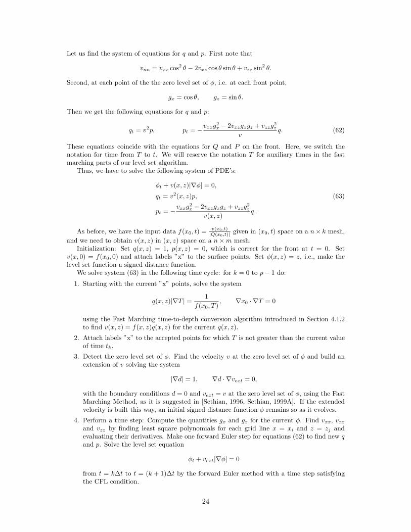
We solve system (63) in the following time cycle: for k = 0 to p− 1 do:

1. Starting with the current ”x” points, solve the system

q(x, z)|∇T | = 1f(x0, T )

, ∇x0 · ∇T = 0

using the Fast Marching time-to-depth conversion algorithm introduced in Section 4.1.2to find v(x, z) = f(x, z)q(x, z) for the current q(x, z).

2. Attach labels ”x” to the accepted points for which T is not greater than the current valueof time tk.

3. Detect the zero level set of φ. Find the velocity v at the zero level set of φ and build anextension of v solving the system

|∇d| = 1, ∇d · ∇vext = 0,

with the boundary conditions d = 0 and vext = v at the zero level set of φ, using the FastMarching Method, as it is suggested in [Sethian, 1996, Sethian, 1999A]. If the extendedvelocity is built this way, an initial signed distance function φ remains so as it evolves.

4. Perform a time step: Compute the quantities gx and gz for the current φ. Find vxx, vxzand vzz by finding least square polynomials for each grid line x = xi and z = zj andevaluating their derivatives. Make one forward Euler step for equations (62) to find new qand p. Solve the level set equation

φt + vext|∇φ| = 0

from t = k∆t to t = (k + 1)∆t by the forward Euler method with a time step satisfyingthe CFL condition.

24

We stress that the main advantage of this algorithm in comparison with the ray tracingalgorithm is that it can work even if the image rays intersect, since it tracks the first arrivalfront.

Having obtained the true seismic velocities v(xi, zj) one can perform depth migration toobtain an improved seismic image in the Cartesian coordinates. Alternatively, knowing the ve-locity v(xi, zj) one can apply Sethian’s fast marching method [Sethian, 1996] to obtain t0(xi, zi)and x0(xi, zi) to convert the time migrated image to depth.

5 Synthetic data examples in 2D

5.1 Example 1

The example in this section allows us to compare performances of the ray tracing algorithm andlevel set algorithm with a somewhat typical approach. One typical approach to seismic velocityestimation is to compute the Dix velocities and then apply image ray tracing. Here we willreplace the image ray tracing with our time-to-depth conversion algorithm.

We considered the velocity fields of the form:

v(x, z) = 1 + exp(−c(x2 + (z − 1)2)

), x0 ∈ [−2, 2], t ∈ [0, 0.7]. (64)

We took c = 0.5, c = 1 and c = 1.5. The larger c, the sharper the Gaussian anomaly. For eachof these fields we created the input data f(x0, t) on a 200× 200 x0× t mesh and applied each ofthe three algorithms to them: the time-to-depth conversion, the ray tracing, and the level set.The output v(x, z) is given on 200× 200 x× z mesh.

The exact velocity, the input data (the Dix velocity, the found velocity and the image raysfor the sharpest Gaussian anomaly corresponding c = 1.5 are shown in Fig. 13. We see that theDix velocity qualitatively differs from the exact velocity and the found velocity resembles theexact velocity much more closely than the Dix velocity.

The results are summarized in Table (1). We see that

Table 1: The maximal relative errors produced by the time-to-depth conversion, the ray tracingand the level set algorithms on the data from the velocity field (64).

Algorithm Time-to-depth Ray tracing Level setc = 0.5 0.31 0.023 0.078c = 1 0.44 0.11 0.079c = 1.5 0.49 0.29 0.20

• the ray tracing and the level set produce significantly more accurate results than the typicalapproach;

• the ray tracing approach is more accurate than the level set where the image rays divergemoderately, while it becomes less accurate as the divergence of the image rays increases.

Note that if the image rays diverge severely so that the derivative vnn (or, in different notations,vqq) becomes large, both our ray tracing and level set algorithms blow up, while the time-to-depth convergence algorithm produces inaccurate but stable results.

25

(a) (b)

(c) (d)

Figure 13: (a): the exact velocity v(x, z); (b) the image rays; (c): the input data f(x0, t) ≡vDix(x0, t); (d): the found velocity v(x, z).

26

5.2 Example 2

In this section we also consider an example with a Gaussian anomaly, but with numbers closerto real seismic data:

v(x, z) = 2 + 2 exp(−(x2 + (z − 2)2)

),

x0 ∈ [−3, 3], t ∈ [0, 1],

The center of the anomaly lies at the depth of 2 km and the background velocity is 2 km/sec.The results (Fig. 14) are produced by the level set algorithm. The found velocity resembles theexact velocity while the Dix velocity and the found velocity differ qualitatively.

(a)

(b)

(c)

Figure 14: (a): the exact velocity v(x, z); (b) the input data: the Dix velocity converted to depthby ”vertical stretch”; (c): the found velocity v(x, z) and the image rays.

6 Field data example

In this section we consider a field data example coming from the North Sea (Fig. 15, left). Themain feature in this image is the salt dome. Typically, the velocity inside the salt is higherthan it is in the surrounding rock. Salt is light and it pushes the layers up as it comes frominside the earth. The lateral velocity variation here is severe according to typical geophysicalsituations. Note rapidly changing values inside the salt dome, which indicate that the lateralvelocity variation is too large for the time migration.

In Fig. 15, right, the time migration velocities chosen in the process of making this imageare shown. Using these time migration velocities, the Dix velocities were then obtained andsmoothed. The level set algorithm was then applied to these Dix velocities to estimate seismicvelocities v(x, z). These seismic velocities together with the image rays computed from the byshooting characteristics are shown in Fig. 16). The depth domain (x, z) was cut at 3.3 km tomake the found v(x, z) into a rectangular matrix.

One can compare the smoothed Dix velocities and the found seismic velocities (Fig. 17) andsee that they differ significantly starting from about 1 km in depth.

The depth migrated image, built using the calculated v(x, z), is shown in Fig. 18 (a). Theimage is in the regular Cartesian coordinates. It shows subsurface structures up to 3.3 km indepth which is quite deep according to geophysical standards. There is a noisy reconstruction

27

Figure 15: Left: seismic image from North Sea obtained by prestack time migration using velocitycontinuation [Fomel, 2003]. Right: the corresponding time migration velocity.

Figure 16: The found seismic velocity v(x, z) and the image rays computed from it.

Figure 17: The smoothed Dix velocity vDix(x0, t0) (left) vs the found seismic velocity v(x, z) (right).

28

inside the salt dome but the surrounding layers are resolved well. Overall, this image looksreasonable.

We applied Sethian’s Fast Marching Method to solve the Eikonal Equation with the foundvelocity v(x, z) and found the matrices t0(x, z) and x0(x, z). Then we converted the timemigrated image in Fig. 15, (left) to depth values using these matrices. The resulting image isshown in Fig. 18 (b). Comparing the two images in depth in Fig. 18 obtained in these twoalternative ways, we see a good agreement between them.

(a) (b)

Figure 18: (a) The poststack depth migrated image obtained with the found v(x, z); (b) Theprestack time migrated image converted to depth.

For comparison, we also used the Dix velocities to perform the depth migration. The resultingimage is shown in Fig. 19, left, while the results of the depth migration with the velocities foundby our level set algorithm are shown in Fig. 19, right. There is a visible change in the lowerpart of the image and several indications that the change is in the right direction.

7 Numerical algorithms in 3D

In this section, we present 3D versions of our algorithms. We present a 3D Dijkstra-like fastmethod for time-to-depth conversion, and a 3D Ray tracing approach for the inverse problem.A 3D level set version is underway.

In more detail, we present a ray tracing approach for solving the inverse problem in 3D (seeSection 3.2). This approach is the extension of the ray tracing approach for 2D (see Section4.2.1). The input data are the set of matrices

F(x0, y0, t0) ≡ ∂K(x0, y0, t0)∂t0

= v2(x, y, z)(QT (x0, y0, t0)Q(x0, y0, t0))−1. (65)

Here v(x, y, z) is the seismic velocity at the location reached by the image being traced backwardsfor time t0 starting from the surface point (x0, y0), and Q(x0, y0, t0) corresponds to the telescopicfamily of rays traced along with the image ray for time t0. The input data are given on the3D time domain mesh (x0i, y0j , t0k), i = 0, ..., nx − 1, j = 0, ..., ny − 1, k = 0, ..., nt − 1,xmin = x00 ≤ x0i ≤ x0,nx−1 = xmax, ymin = y00 ≤ y0j ≤ y0,ny−1 = ymax, 0 = t0 ≤tk ≤ tnt−1 = tmax. The output is the four sets of data v(x, y, z), t0(x, y, z), x0(x, y, z) andy0(x, y, z) given on the 3D depth domain mesh (xi, yy, zk), i = 0, ..., nx − 1, j = 0, ..., ny − 1,k = 0, ..., nz − 1, xmin = x0 ≤ xi ≤ xnx−1 = xmax, ymin = y0 ≤ yj ≤ yny−1 = ymax,0 = z0 ≤ zk ≤ znz−1 = zmax.

29

Figure 19: The poststack depth migration using the Dix velocities (left) vs the poststack depthmigration using the estimated seismic velocities (right).

This approach consists of the following three steps.Step 1. Ray tracing algorithm which computes the image rays the image rays.Step 2. Using the image rays found in Step 1, compute the geometrical spreading which

equals |detQ| ([Popov, 2002]) and determine the velocity v(x0, y0, t0) from the input data 65.Step 3. Convert the velocities v(x0, y0, t0) given in the time coordinates (x0, y0, t0) to depth:

find v(x, y, z).Now let us describe each of these three steps in details.

30

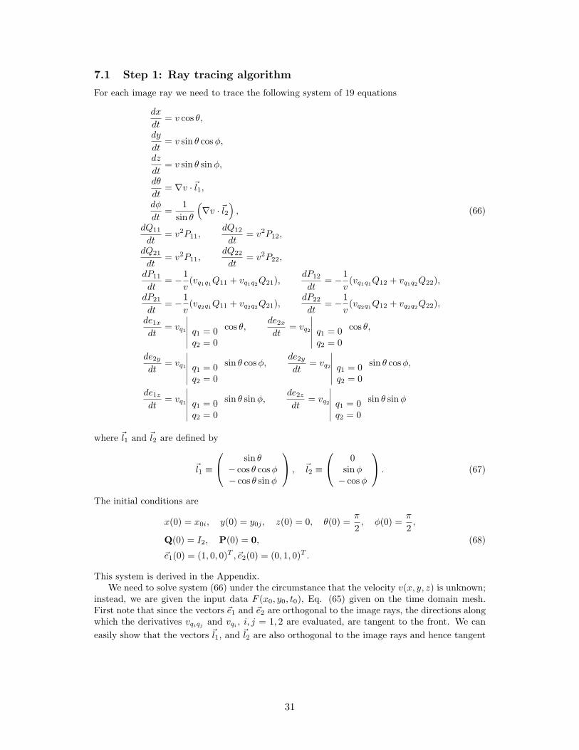
7.1 Step 1: Ray tracing algorithm

For each image ray we need to trace the following system of 19 equations

dx

dt= v cos θ,

dy

dt= v sin θ cosφ,

dz

dt= v sin θ sinφ,

dθ

dt= ∇v ·~l1,

dφ

dt=

1sin θ

(∇v ·~l2

), (66)

dQ11

dt= v2P11,

dQ12

dt= v2P12,

dQ21

dt= v2P11,

dQ22

dt= v2P22,

dP11

dt= −1

v(vq1q1Q11 + vq1q2Q21),

dP12

dt= −1

v(vq1q1Q12 + vq1q2Q22),

dP21

dt= −1

v(vq2q1Q11 + vq2q2Q21),

dP22

dt= −1

v(vq2q1Q12 + vq2q2Q22),

de1xdt

= vq1 q1 = 0q2 = 0

cos θ,de2xdt

= vq2 q1 = 0q2 = 0

cos θ,

de2ydt

= vq1 q1 = 0q2 = 0

sin θ cosφ,de2ydt

= vq2 q1 = 0q2 = 0

sin θ cosφ,

de1zdt

= vq1 q1 = 0q2 = 0

sin θ sinφ,de2zdt

= vq2 q1 = 0q2 = 0

sin θ sinφ

where ~l1 and ~l2 are defined by

~l1 ≡

sin θ− cos θ cosφ− cos θ sinφ

, ~l2 ≡

0sinφ− cosφ

. (67)

The initial conditions are

x(0) = x0i, y(0) = y0j , z(0) = 0, θ(0) =π

2, φ(0) =

π

2,

Q(0) = I2, P(0) = 0, (68)

~e1(0) = (1, 0, 0)T , ~e2(0) = (0, 1, 0)T .

This system is derived in the Appendix.We need to solve system (66) under the circumstance that the velocity v(x, y, z) is unknown;

instead, we are given the input data F (x0, y0, t0), Eq. (65) given on the time domain mesh.First note that since the vectors ~e1 and ~e2 are orthogonal to the image rays, the directions alongwhich the derivatives vqiqj

and vqi, i, j = 1, 2 are evaluated, are tangent to the front. We can

easily show that the vectors ~l1, and ~l2 are also orthogonal to the image rays and hence tangent

31

to the front. Let ~τ be a unit tangent vector to the image ray. Then

~l1 · ~τ =

sin θ− cos θ cosφ− cos θ sinφ

· cos θ

sin θ cosφsin θ sinφ

= 0,

~l2 · ~τ =

0sinφ− cosφ

· cos θ

sin θ cosφsin θ sinφ

= 0.

Thus, all of the directions along which we need to evaluate the derivatives of the velocity aretangent to the front.

It was shown by [Adalsteinsson and Sethian, 2002] that for a flat curve the following relationtakes place:

vss = vqq − vτκ, (69)

where vss is the second derivative along the curve, vqq is the second derivative along the tangentline, vτ is the derivative along the normal direction to the curve, and κ is the curvature of thecurve. The relation (69) is valid for a nonflat curve as well, and the proof is identical:

Proof Let (x(s), y(s), z(s)) be a curve, and l be the natural parameter along it - the arc length.Let ~e =

(dxds ,

dyds ,

dzds

)be its velocity vector, which is the unit vector tangent to it. Then the

curvature κ is(d2xds2 ,

d2yds2 ,

d2zds2

). Differentiate v twice with respect to the arc length:

vss =∂

∂s

(∂

∂sv(x(s), y(s), z(s))

)=

∂

∂s(vxex + vyey + vzez)

=∂

∂s(∇v · ~e) =

(∂

∂s∇v)· ~e+∇v · ∂~e

∂s

=(~e)TD2v~e− κ∇v · ~n = vqq − vτκ,

as we wanted to prove. Here D2v is the matrix of the second derivatives of v.

Now we are ready to present the ray tracing algorithm. Since the matrix Q at the surface is

the identity matrix, F(x0, y0, 0) =(v2 00 v2

), we can evaluate the velocity at the surface by

v(x0, y0, 0) = 4√

F11F22. (70)

Then we make the first forward Euler time step for system (66) using the initial conditions (68)and taking into account that x ≡ q1 and y ≡ q2 at the surface. We then find the velocity at thenext moment of time t1 by

v(x0, y0, t1) = 4√

det F(x0, y0, t1)(det Q(x0, y0, t1)2.

The further time steps are given by the following:

For k = 1 to nt − 2 do

1. Estimate the curvatures of the grid curves (x0, y0j , tk), j = const, and (x0i, y0, tk), i =const and estimate the first and the second derivatives of the velocity along the tangentlines to these curves. We first approximate the functions x(x0, y0j , tk), y(x0, y0j , tk) andz(x0, y0j , tk) by a least squares polynomial and find its second derivatives with respect tothe arc length s1. Then approximate the velocity along these lines using a least squarespolynomial and evaluate its the first and the second derivatives with respect to the arclength s1. Correct the second derivatives using formula (69). Repeat this procedure forthe grid curves (x0i, y0, tk) and also find the mixed second derivative of v ∂2v

∂s1∂s2.

32

2. We have estimated the first and the second derivatives of v along the tangent lines to thegrid curves: vs1 , vs2 , vs1s1 , vs2s2 and vs1s2 . We need to find the derivatives of the velocityalong the directions ~e1, ~e2, ~l1 and ~l2. As we have shown, all of these directions are tangentto the front, hence they lie in the same plane as the directions s1 and s2. We expressthese directions in terms of s1 and s2 using the least squares and then find the neededderivatives. Let ~s1 and ~s2 be unit vectors in the directions s1 and s2. Let

~e1 = b11~s1 + b12~s2, (71)~e2 = b21 ~s1 + b22~s2,

therefore,

vq1 = ~e1 · ∇v = (b11~s1 + b12~s2) · ∇v = b11vs1 + b12vs2 , (72)vq2 = ~e2 · ∇v = (b21~s1 + b22~s2) · ∇v = b21vs1 + b22vs2 .

Similarly we find ~li · ∇v, i = 1, 2. We compute the matrix (vqiqj )i,j=1,2 as follows.

vqiqj = (~ei)TD2v~ej = (bi1~s1 + bi2~s2)TD2v(bj1~s1 + bj2~s2) (73)

= (bi1bi2)(

(~s1)T

(~s2)T

)D2v(~s1~s2)

(bj1bj2

).

Therefore,

V ≡(

∂2v

∂qi∂qj

)i,j=1,2

= B

(∂v

∂si∂sj

)BT , (74)

where B =(b11 b12b21 b22

).

3. Perform the Euler step for system (66).

4. Using the matrices Q(x0, y0, tk+1), find v(x0, y0, tk+1):

v(x0, y0, tk+1) = 4√

det F(x0, y0, tk+1)(det Q(x0, y0, tk+1))2. (75)

7.2 Step 2: Recomputation of the velocity using the found image rays

The ray tracing algorithm outlined in the previous section computes the image rays significantlymore accurately than it estimates the velocity v(x0, y0, t0). This gives us an opportunity to re-compute the velocity more accurately using the found image rays. It was shown in [Popov, 2002]that the geometrical spreading of the rays equals |det Q|. We estimate the it as the ratio of theareas of the grid cells at time t = tk and at t = 0 and then compute the velocity by formula(75).

7.3 Step 3: Time-to-depth conversion algorithm

The motivation and the main building block for this algorithm is Sethian’s fast marching method(see [Sethian, 1996]). It is a 3D upgrade of the time-to-depth conversion algorithm presentedin Section 4.1. In this section, we will work with the slowness s, the reciprocal of the velocityv, for convenience. Also we switch the notation for time from t0 to T to be consistent with thenotations in the Eikonal equation and Section 4.1.

We are given s(x0, y0, T ). We want to find s(x, y, z), x0(x, y, z), y0(x, y, z), T (x, y, z). Thesefunctions relate according to the following system of PDE’s:

|∇T |2 = s2(x0(x, y, z), y0(x, y, z), T (x, y, z)),∇x0 · ∇T = 0, (76)∇y0 · ∇T = 0.

33

The first equation is the Eikonal equation with an unknown right-hand-side. The other twoare the orthogonality relations reflecting that the image rays are orthogonal to the equi-timesurfaces. The derivation of these orthogonality relations is based on the fact that x0 and y0remain unchanged along the image rays and is very similar to the derivation of the orthogonalityrelation (56) in Section 4.1.1 for the 2D case.

The numerical algorithm for solving system (76) is very similar to the one described in Sec-tion 4.1.2, except for the 3-point update which must be added in the 3D case. The computationalcost is O(N3 logN), which is the same as for the 3D fast marching method. The equations for 1-, 2- and 3-point update are the following. Suppose we need to find s, x0,y0 and T at the point P .

1. 1-point-update. Let A be the a known nearest neighbor of P , and there are no knownneighbors of P lying on the other grid lines. ha can be any of hx, hy, hz, depending onwhich grid line the points P and A lie on.

T (P )− T (A)ha

= s(x0(A), y0(A), T (P )). (77)

2. 2-point-update. Let A and B be two known nearest neighbors of P lying on different gridlines, and there is no known nearest neighbor lying on the other grid line. ha and hb canbe any pair of different symbols of hx, hy, hz, depending on the arrangement of the pointsP , A and B.

(T (P )− T (A))2

h2a

+(T (P )− T (B))2

h2b

= s2(x0(P ), y0(P ), T (P )),

(T (P )− T (A))(x0(P )− x0(A))h2a

+(T (P )− T (B))(x0(P )− x0(B))

h2b

= 0,

(T (P )− T (A))(y0(P )− y0(A))h2a

+(T (P )− T (B))(y0(P )− y0(B))

h2b

= 0, (78)

s(P ) = s(x0(P ), y0(P ), T (P )),T (P ) ≥ max{T (A), T (B)}, x1 ≤ x0(P ) ≤ x2, y1 ≤ y0(P ) ≤ y2,

where x1 = min{x0(A), x0(B)}, x2 = max{x0(A), x0(B)}, y1 = min{y0(A), y0(B)}, y2 =max{y0(A), y0(B)}.

3. 3-point-update. Let A, B and C be three known neighbors of P all lying on different gridlines. ha, hb, hc is any permutation of hx, hy, hz.

(T (P )− T (A))2

h2a

+(T (P )− T (B))2

h2b

+(T (P )− T (C))2

h2c

= s2(x0(P ), y0(P ), T (P )),

(T (P )− T (A))(x0(P )− x0(A))h2a

+(T (P )− T (B))(x0(P )− x0(B))

h2b

+(T (P )− T (C))(x0(P )− x0(C))

h2c

= 0, (79)

(T (P )− T (A))(y0(P )− y0(A))h2a

+(T (P )− T (B))(y0(P )− y0(B))

h2b

+(T (P )− T (C))(y0(P )− y0(C))

h2c

= 0.

s(P ) = s(x0(P ), y0(P ), T (P )),T (P ) ≥ max{T (A), T (B, T (C))}, x1 ≤ x0(P ) ≤ x2, y1 ≤ y0(P ) ≤ y2,

where x1 = min{x0(A), x0(B, x0(C))}, x2 = max{x0(A), x0(B), x0(C)}, y1 = min{y0(A), y0(B), y0(C)},y2 = max{y0(A), y0(B), y0(C)}.

34

Note that whenever we use the 1-point update, we artificially put the point P on the imageray passing through the point A. Whenever we use the 2-point-update, we artificially create asymmetry with respect to a plane (ABP ). Taking this into account, we accept the followingupdate rule: 2-point-update replaces 1-point-update and 3-point-update replaces 2-point-updatewhenever it is possible. This algorithm has the same hypothetical causality issue as its 2Dversion (see Section 4.1.3). We have not encounter any causality violation in our numericalexperiments. This causality issue is the subject of our future research.

In order to avoid the boundary effects (see Section 4.1.4), no image ray may enter the domain[xmin, xmax]× [ymin, ymax]× [0, zmax] through the side faces. That is, the boundary image raysmust be either straight or leave the domain and never re-enter.

8 Synthetic data examples in 3D

In this section we demonstrate the ray tracing approach in 3D.

8.1 Example 1

Consider the following velocity field with the background velocity of 1.5 km/sec and a Gaussiananomaly centered at the depth of 2 km:

v(x, y, z) = 1.5 + exp (−0.2(x2 + y2)− 0.3(z − 2)2). (80)

First we create the input F (x0, y0, t0) (see Eq. (65)), by shooting characteristics and solvingsystem Eq. (66) in the time domain

xmin = −5 km ≤ x0 ≤ xmax = 5 km, ymin = −5 km ≤ y0 ≤ ymax = 5 km, (81)0 ≤ t0 ≤ tmax = 2 sec

on the 50 × 50 × 50 nx × ny × nt mesh. Then we apply consequently first the ray tracingalgorithm to find the velocities v(x0, y0, t0) from the matrices F(x0, y0, t0) and then the time-to-depth conversion algorithm to find the velocity in the depth coordinates v(x, y, z) from thevelocity in the time coordinates v(x0, y0, t0). We obtain the output in the depth domain

xmin = −5 km ≤ x ≤ xmax = 5 km, ymin = −5 km ≤ y ≤ ymax = 5 km, (82)0 ≤ z ≤ zmax = 3.409 km

on the 50× 50× 40 nx × ny × nz mesh.In 2D we compared the results of our approaches with the results of the Dix inversion

converted to the depth domain. The results indicate that the algorithms improve the Dixinversion and that our approaches can do qualitatively better than the Dix inversion. We wouldlike to have something to compare the results of our ray tracing approach in 3D as well. Wetake the following heuristic estimate of the velocity:

vheur = 4√

det F, (83)

which is a 3D analog of the Dix velocity in 2D, and convert it to depth using our time-to-depthconversion algorithm.

The results are presented in Fig. 20. The velocity v(x, y, z) is shown at the depths of 87.4 m,262.2 m, 437.0 m, ..., 3408.6 m, the interval between slices is 174.8 m. At each depth, the darkblue color corresponds to v = 1.5 km/sec, and the dark red color corresponds to v = 2.5 km/sec.The exact velocity is shown in Fig. 20(a). The velocity recovered by our ray tracing approach isshown in Fig. 20(b). The heuristic estimate of the velocity (see. Eq. (83)) converted to depthis shown in Fig. 20(c). The image rays projected onto the surface are shown in Fig. 20(d).

First, we note that we were able to obtain a velocity estimate below the center of theGaussian anomaly using our ray tracing approach. Second, up to the depth where the center ofthe anomaly lies, our results are quite accurate. Third, throughout all the depth domain, ourvelocity is more accurate, and in the medium depths even qualitatively more accurate than theheuristic estimate analogous to the Dix inversion.

35

(a) (b)

(c) (d)

Figure 20: Example 1. (a) The exact velocity; (b) the velocity found by our ray tracing approach;(c) the heuristic estimate estimate analogous to the Dix inversion, converted to depth; (d) theimage rays projected onto the earth surface.

36

8.2 Example 2

In this example, we also consider a velocity field with a Gaussian anomaly centered at the depthof 2 km, but with smaller variances:

v(x, y, z) = 1.5 + exp (−0.5x2 − 0.3 ∗ y2 − 0.3(z − 2)2). (84)

The input data are computed in the time domain

xmin = −3 km ≤ x0 ≤ xmax = 3 km, ymin = −3 km ≤ y0 ≤ ymax = 3 km, (85)0 ≤ t0 ≤ tmax = 2 sec

on a 50× 50× 50 nx × ny × nt mesh. The output is computed in the depth domain

xmin = −3 km ≤ x ≤ xmax = 3 km, ymin = −3 km ≤ y ≤ ymax = 3 km, (86)0 ≤ z ≤ zmax = 1.6568 km

on a 50×50×20 nx×ny×nz mesh. The results are presented in Fig. 21. The velocity is shownat the depths of from 0 to zmax = 1.6568 km at every 87.2 m. At each depth, the dark bluecolor corresponds to v = 1.5 km/sec, and the dark red color corresponds to v = 2.5 km/sec.The exact velocity is shown in Fig. 21(a). The velocity recovered by our ray tracing approach isshown in Fig. 21(b). The heuristic estimate of the velocity (see. Eq. (83)) converted to depthis shown in Fig. 21(c). The image rays projected onto the surface are shown in Fig. 21(d).

We see that the velocity recovered by our ray tracing approach is similar to the exact velocitywhile the heuristic estimate is qualitatively different.

8.3 Example 3

In this example, we consider a velocity field, Gaussian in z and star shaped in (x, y). We buildthis field as follows. We take a closed curve shaped as a three tip star given by

α0 = φ− 0.2 cos(3φ); (87)r0 = 1− 0.1 cos(3φ).

Then for every point of this curve with polar coordinates (r0, α0) consider a spiral line definedby

r = r0 + 4σ; (88)α = α0 + 0.11σ.

The velocity at every point (x, y) is defined by

v(x, y) = 1.5 + exp

(−0.1

(d

r0

)2).

d is the distance from the geometrical center of the level sets located at (xc = 0, yc = 0). r0 is thenormalizing factor which is found from equations (87), (88). We equate r = d and α = arg(x, y)and solve for r0, α0, φ and σ. Then we define v(x, y, z) by

v(x, y, z) = 1.5 + exp

(−0.1

(d

r0

)2

− 0.5(z − 2)2). (89)

The input data are computed in the time domain

xmin = −8 km ≤ x0 ≤ xmax = 8 km, ymin = −8 km ≤ y0 ≤ ymax = 8 km, (90)0 ≤ t0 ≤ tmax = 1.5 sec

37

(a) (b)

(c) (d)

Figure 21: Example 2. (a) The exact velocity; (b) the velocity found by our ray tracing approach;(c) the heuristic estimate estimate analogous to the Dix inversion, converted to depth; (d) theimage rays projected onto the earth surface.

38

on a 50× 50× 50 nx × ny × nt mesh. The output is computed in the depth domain

xmin = −8 km ≤ x ≤ xmax = 8 km, ymin = −8 km ≤ y ≤ ymax = 8 km, (91)0 ≤ z ≤ zmax = 2.027 km

on a 50 × 50 × 32 nx × ny × nz mesh. The results are presented in Fig. 22. The velocity isshown at depths of 65.4 m, 196.2 m, 327.0 m, ...,2027 m. The interval between the slices is130.8 m. At each depth, the dark blue color corresponds to v = 1.5 km/sec, and the dark redcolor corresponds to v = 2.5 km/sec. The exact velocity is shown in Fig. 22(a). The velocityrecovered by our ray tracing approach is shown in Fig. 22(b). The heuristic estimate of thevelocity (see. Eq. (83)) converted to depth is shown in Fig. 22(c). The image rays projectedonto the surface are shown in Fig. 22(d).

(a) (b)

(c) (d)

Figure 22: Example 3. (a) The exact velocity; (b) the velocity found by our ray tracing approach;(c) the heuristic estimate estimate analogous to the Dix inversion, converted to depth; (d) theimage rays projected onto the earth surface.

The anomaly in this example has a nontrivial geometry. The velocity found by our raytracing approach transfers the geometry qualitatively correctly, while the heuristic estimatefails to do so.

39

9 Conclusions

We derived a theoretical relation between the Dix velocities in time migration coordinates andthe true seismic velocities in the depth coordinates in 2D, and a relation between the matricesF(x0, y0, t0), which can be determined from the time migration, and the true seismic velocitiesin the depth coordinated in 3D.

We stated the corresponding inverse problem in 2D and 3D. We showed that the inverseproblem is ill-posed, i.e. sensitive to small perturbations.

Nonetheless we attempted a regularized reconstruction and developed numerical algorithmsin 2D and 3D for obtaining smoothed seismic velocities.

We tested our algorithms on a collection of synthetic 2D and 3D examples and demonstratedthat they recover the seismic velocity significantly more accurately than the Dix inversion, whichis the standard estimate. Moreover, the Dix velocity may qualitatively differ from the truevelocity.

We applied our level set algorithm to a field data with severe lateral velocity variation andfound an estimate of the seismic velocity as well as the transition matrices from time migrationcoordinates to depth coordinates up to 3.3 km in depth. We used this velocity to obtain a depthmigrated image. We also used these transition matrices to convert the time migrated image todepth. We got a good agreement between these two images. We also used the Dix velocitiesto produce a depth migrated image. The image obtained using the velocities estimated by ourapproach, and the image obtained using the Dix velocities noticeably differ in their lower part.There are several indications that the application of our approach made the change in rightdirection.

References

[Adalsteinsson and Sethian, 2002] Adalsteinsson, D. and Sethian, J.A., Transport and Diffusionof Material Quantities on Propagating Interfaces via Level Set Methods, J. Comp. Phys, 185,1, pp. 271-288, 2002.

[Cerveny, 2001] Cerveny, V., Seismic Ray Theory: Cambridge University Press, 2001.[Dix, 1955] Dix, C. H., Seismic velocities from surface measurements: Geophysics, 20, pp. 68-86,

1955[Fomel, 2003] Fomel, S., Time-migration velocity analysis by velocity continuation: Geophysics,

68, pp. 1662-1672, 2003[Hubral, 1977] Hubral, P., Time migration - Some ray theoretical aspects: Geophys. Prosp., 25,

pp. 738-745, 1977[Hubral and Krey, 1980] Hubral, P., Krey, T., Interval velocities from seismic reflection time

measurements: SEG, 1980.[Osher and Sethian, 1988] Osher S., Sethian, J. A., Front propagating with curvature dependent

speed: algorithms based on Hamilton-Jacobi formulations, J. Comp. Phys., 79, pp. 12-49,1988.

[Popov, 2002] Popov, M. M., Ray theory and gaussian beam method for geophysicists: Salvador:EDUFBA, 2002.

[Popov and Psencik, 1978] Popov, M. M, Psencik, I., Computation of ray amplitudes in inho-mogeneous media with curved interfaces: Studia Geoph. et Geod., 22, pp. 248-258, 1978.

[Sethian, 1982] Sethian, J. A., An Analysis of Flame Propagation: Ph.D. Dissertation, Depart-ment of Mathematics, University of California, Berkeley, CA, 1982.

[Sethian, 1985] Sethian, J. A., Curvature and the Evolution of Fronts: Commun. in Math.Phys., 101, pp. 487-499, 1985.

[Sethian, 1987] Sethian, J. A., Numerical methods for propagating fronts in Variational Methodsfor Free Surface Interfaces, (eds. P. Concus & R. Finn), Springer-Verlag, NY, 1987.

40

[Sethian, 1996] Sethian , J. A., A Fast Marching Level Set Method for Monotonically AdvancingFronts: Proceedings of the National Academy of Sciences, 93, 4, 1996.

[Sethian, 1999A] Sethian, J.A., Fast Marching Methods: SIAM Review, Vol. 41, No. 2, pp.199-235, 1999.

[Sethian, 1999B] Sethian, J. A., Level set methods and fast marching methods: CambridgeUniversity Press, 1999.

[Sethian and Vladimirsky, 2003] Sethian, J. A., Vladimirsky, A., Ordered Upwind Methods forStatic Hamilton-Jacobi Equations: Theory and Algorithms: SIAM J. Numer. Anal., 41, 1,pp. 325-363, 2003

[Shah, 1973] Shah, P. M., Use of wavefront curvature to relate seismic data with subsurfaceparameters: Geophysics, 38, 812-825, 1973.

[Tsitsiklis, 1995] Tsitsiklis, J.N., Efficient Algorithms for Globally Optimal Trajectories: IEEETran. Automatic Control, 40, pp. 1528-1538, 1995.

[Yilmaz, 2001] Yilmaz, O., Seismic Data Analysis: Soc. of Expl. Geophys., 2001

APPENDIX: Derivation of 3D Ray-Tracing Equations

At each moment of time t, we will describe a ray by the following five coordinates: x(t), y(t),z(t), θ(t), φ(t), where θ is the angle between the direction of the ray and the x-axis, and φ is theangle between the projection of the ray onto yz-plane and the positive direction of the y-axis.We start to trace the image rays from the surface normal to it. Our choice of angles allows usto avoid (or, at least, substantially postpone) the problem of φ being undefined where θ = 0.As before, define the Hamiltonian by

H =12(|∇t|2 − s2(x, y, z)

)≡ 1

2(|~p|2 − s2(x, y, z)

)≡ 0, (A-1)

where s is the slowness - the reciprocal of the velocity. Then the ray equations in the Hamiltonianform are

dx

dσ= px,

dpxdσ

= ssx,

dy

dσ= py,

dpydσ

= ssy, (A-2)

dz

dσ= pz,

dpzdσ

= ssz.

Then we introduce

θ = arctan

√p2y + p2

z

px, φ = arctan

pzpy, (A-3)

and perform the variable change in system A-2.

dθ

dσ=

dθ

dpx

dpxdσ

+dθ

dpy

dpydσ

+dθ

dpz

dpzdσ

(A-4)

=1

1 + p2y+p2zp2x

−√p2y + p2

z

p2x

ssx +py

px√p2y + p2

z

ssy +pz

px√p2y + p2

z

ssz

.

Then, using the relations

px = s cos θ, py = s sin θ cosφ, pz = s sin θ sinφ, p2y + p2

z = s sin θ, (A-5)

41

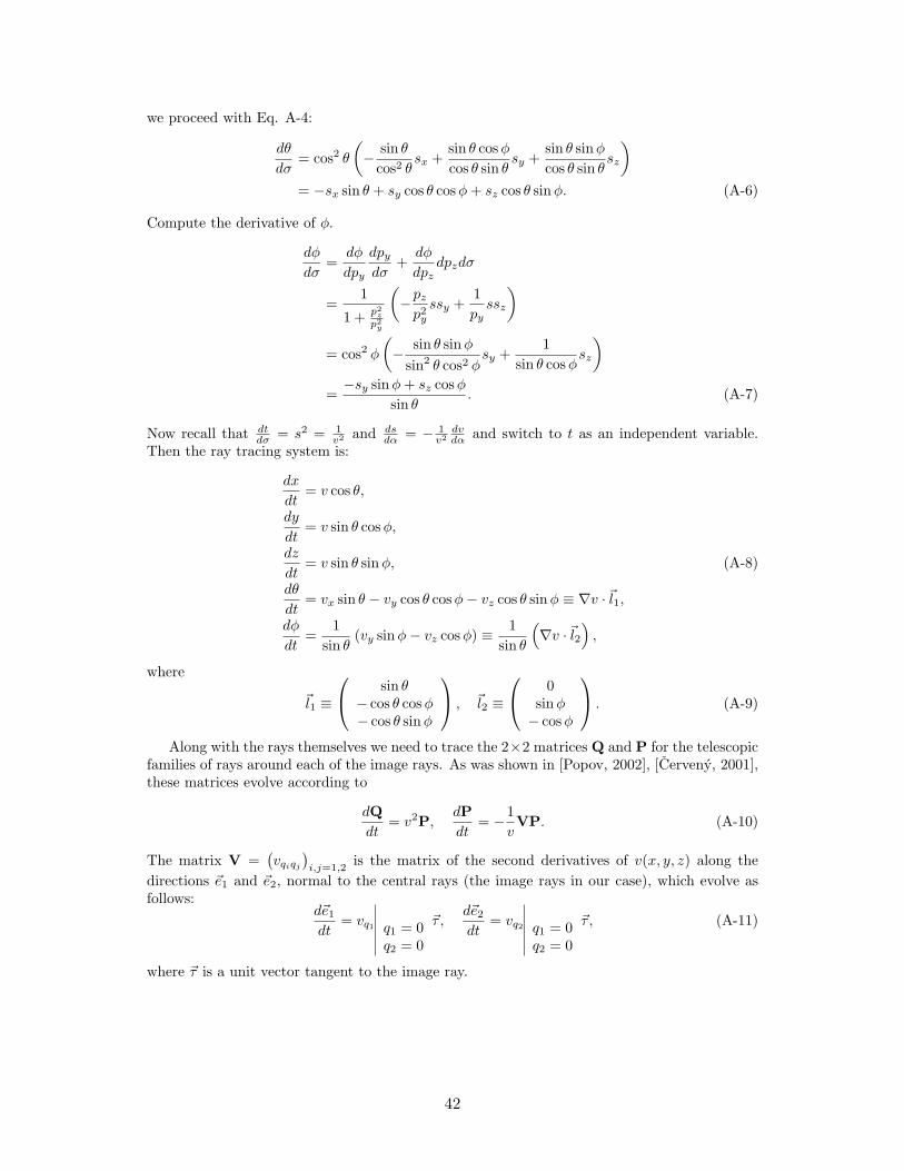
we proceed with Eq. A-4:

dθ

dσ= cos2 θ

(− sin θ

cos2 θsx +

sin θ cosφcos θ sin θ

sy +sin θ sinφcos θ sin θ

sz

)= −sx sin θ + sy cos θ cosφ+ sz cos θ sinφ. (A-6)

Compute the derivative of φ.

dφ

dσ=

dφ

dpy

dpydσ

+dφ

dpzdpzdσ

=1

1 + p2zp2y

(−pzp2y

ssy +1pyssz

)

= cos2 φ(− sin θ sinφ

sin2 θ cos2 φsy +

1sin θ cosφ

sz

)=−sy sinφ+ sz cosφ

sin θ. (A-7)

Now recall that dtdσ = s2 = 1

v2 and dsdα = − 1

v2dvdα and switch to t as an independent variable.

Then the ray tracing system is:

dx

dt= v cos θ,

dy

dt= v sin θ cosφ,

dz

dt= v sin θ sinφ, (A-8)

dθ

dt= vx sin θ − vy cos θ cosφ− vz cos θ sinφ ≡ ∇v ·~l1,

dφ

dt=

1sin θ

(vy sinφ− vz cosφ) ≡ 1sin θ

(∇v ·~l2

),

where

~l1 ≡

sin θ− cos θ cosφ− cos θ sinφ

, ~l2 ≡

0sinφ− cosφ

. (A-9)

Along with the rays themselves we need to trace the 2×2 matrices Q and P for the telescopicfamilies of rays around each of the image rays. As was shown in [Popov, 2002], [Cerveny, 2001],these matrices evolve according to

dQdt

= v2P,dPdt

= −1v

VP. (A-10)

The matrix V =(vqiqj

)i,j=1,2

is the matrix of the second derivatives of v(x, y, z) along thedirections ~e1 and ~e2, normal to the central rays (the image rays in our case), which evolve asfollows:

d~e1dt

= vq1 q1 = 0q2 = 0

~τ ,d~e2dt

= vq2 q1 = 0q2 = 0

~τ , (A-11)

where ~τ is a unit vector tangent to the image ray.

42