STAFFING A CALL CENTERWITH UNCERTAIN ARRIVAL RATE AND ABSENTEEISM

by

Ward Whitt

Department of Industrial Engineering and Operations ResearchColumbia University, New York, NY 10027–6699

phone: 212-854-7255; fax: 212-854-8103; email: ww2040@columbia.edu

Abstract

This paper proposes simple methods for staffing a single-class call center with uncertain arrival

rate and uncertain staffing due to employee absenteeism. The arrival rate and the proportion

of servers present are treated as random variables. The basic model is a multi-server queue

with customer abandonment, allowing non-exponential service-time and time-to-abandon dis-

tributions. The goal is to maximize the expected net return, given throughput benefit and

server, customer-abandonment and customer-waiting costs, but attention is also given to the

standard deviation of the return. The approach is to approximate the performance and the net

return, conditional on the random model-parameter vector, and then uncondition to get the

desired results. Two recently-developed approximations are used for the conditional perfor-

mance measures: first, a deterministic fluid approximation and, second, a numerical algorithm

based on a purely Markovian birth-and-death model, having state-dependent death rates.

Keywords: model-parameter uncertainty, contact centers, employee absenteeism, customer

abandonment, fluid models.

Submitted: February 2005; Revision submitted and accepted: August 2005

Final prepublication version: December 2005

1. Introduction

For the design and management of telephone call centers and many other service systems,

it is common to use stochastic models such as the Erlang delay model, which capture the

uncertainty associated with arrivals and service times. When we apply those stochastic models,

we usually assume that key model parameters such as the arrival rate and the number of

servers are known. Then we typically describe the congestion resulting from stochastic-process

variability given these assumed model parameters. However, in practice, there often not only

is the usual uncertainty (fluctuations) captured by stochastic-process variability, but there

also is uncertainty about the model parameters. For a given model, this issue is commonly

addressed by doing sensitivity analysis, i.e., by describing the congestion stemming from a

variety of possible model parameters. Sensitivity analysis gives important insight, but it does

not present a unified approach, simultaneously taking into account all forms of uncertainty.

The purpose of this paper is to introduce a model, and methods for analyzing that model,

that directly address the uncertainty in the model parameters as well as the stochastic-process

variability in the model for given model parameters.

Even though model-parameter uncertainty has not received much attention in the analysis

of call-center performance, it is a well recognized problem with a long history; e.g., see Helton

and Burmaster (1996), Henderson (2003), Palm (1993) and Plum (1986). Researchers have

been investigating the extent of model-parameter uncertainty in contact centers and how to

reduce it with better forecasting; e.g., see Avramidis et al. (2004), Brown et al. (2005),

Shen and Huang (2005) and references therein. Other researchers are also investigating ways

to cope with model-parameter uncertainty in contact centers; see Bassamboo et al. (2006a,

b), Harrison and Zeevi (2005), Jongbloed and Koole (2001) and Steckley et al. (2004). Our

approach is most closely related to Harrison and Zeevi (2005) and Bassamboo et al. (2006a, b)

because, like them, we exploit a deterministic fluid model, but we use a different fluid model

- the fluid model from Whitt (2005b) - which captures the impact of non-exponential service-

time and time-to-abandon distributions beyond their means. (On the other hand, Harrison

and Zeevi (2005) and Bassamboo et al. (2006a,b) treat a multi-class call-center model with

skill-based routing.) We also present a numerical method based on Whitt (2005a), which can

be used to evaluate the performance of the fluid model as well as be applied directly.

The specific model we consider is a general multi-server queue with customer abandon-

ments. Motivated by the application to call centers, we focus on the case where there is a

1

relatively large arrival rate and a large number of servers; see Gans et al. (2003) for back-

ground. Most call centers serve multiple classes of customers, using multiple pools of servers,

by means of skill-based routing. However, here we consider only the basic single-class special

case. In particular, we consider the M/GI/s + GI queueing model, having a Poisson arrival

process, independent and identically distributed (IID) service times with a general distribu-

tion (the first GI), s servers, unlimited waiting space, IID times to abandon with a general

distribution (the +GI) and the first-come first-served service discipline. Each customer who

cannot start service immediately upon arrival waits in queue, and if service has not begun

by that customer’s randomly selected time to abandon, that customer abandons, i.e., leaves

without receiving service, and without affecting the future arrival process. (We do not consider

retrials.) Because we restrict attention to single-class call centers, the results here will not be

directly applicable to many current call centers, but nevertheless we think the present analysis

can provide useful insight. Similar analyses may be possible for more realistic systems.

Our uncertainty about the model is represented by a random vector (Λ,Γ), which takes

values in (0,∞)×(0, 1]. (The intervals are open on the left to rule out 0 as a possible value.) The

first random variable Λ is the arrival rate, while the second random variable Γ is the proportion

of the s servers that are present. Since we are thinking of large s, typically assuming values

of 100 or more, we ignore the natural integrality requirement on the number of servers; i.e.,

we let the number of servers be dΓse, the smallest integer greater than or equal to Γs. (This

assumption can easily be modified.) We are motivated to let the number of servers be random

because scheduled service representatives may fail to show up due to absenteeism.

We assume that the random arrival rate Λ and the random number of servers Γs operates

throughout a time period in which we would be using the steady-state distribution of the

M/GI/s + GI queueing model to describe system performance. For example, that might be a

half hour for a call center with service times averaging about 5 minutes. We assume that the

arrival rate is constant throughout that half hour, but its actual value is random. We achieve

that by letting the actual number of arrivals in an interval [0, t] be

A(t) ≡ A1(Λt), t ≥ 0 , (1.1)

where A1 ≡ {A1(t) : t ≥ 0} is a given rate-1 Poisson process. That makes A a so-called Cox

process with random rate Λ. Conditional on Λ = λ, A is a rate-λ Poisson process.

Our model uncertainty is limited to two elements: the arrival rate and the number of

servers. There are also other model elements about which we could be uncertain, but the

2

two we consider seem especially appropriate for customary call-center applications. Because

of the large number of customers served in a call center, there is less likely to be substantial

uncertainty about the distributions of customer service times and times to abandon. However,

the methods in this paper can be applied to study uncertainty of other model elements.

For this model, our goal is threefold: We want to (i) obtain useful simple approximate per-

formance descriptions, (ii) perform optimization to determine staffing levels that approximately

maximize the expected net return or revenue, given general throughput-benefit, server-cost,

abandonment-cost and customer-waiting-cost functions, and (iii) improve our understanding

of model-parameter uncertainty (e.g., assess its consequences).

Our approach is to approximate performance, and subsequently, the net return, conditional

on observing a particular realization (λ, γ) of the random vector (Λ, Γ), and then integrate out

the uncertainty in (Λ,Γ). For each realization (λ, γ) of (Λ,Γ), we have a conventional M/GI/s+

GI queue, for which there are steady-state performance measures, depending on (λ, γ). We

then uncondition (average with respect to (Λ,Γ)) to describe the overall performance. For

example, the overall expected kth moment of the steady-state waiting time, as a function of

the number of servers s, is defined by

E[W (s)k] =∫

(0,∞)×(0,1]E[W (s)k|(Λ,Γ) = (λ, γ)] dP ((Λ, Γ) = (λ, γ)) , (1.2)

where E[W (s)k|(Λ, Γ) = (λ, γ)] is the conventional kth moment of the steady-state waiting

time in the model with model parameters (Λ, Γ) = (λ, γ).

As indicated, we average over the performance metrics and expected rewards obtained for

each candidate value (λ, γ) of the random vector (Λ,Γ), using an assumed probability distri-

bution for the random vector (Λ, Γ). That yields an overall expected performance and overall

expected reward. In addition, we compute the overall standard deviation of the performance

measure and the total return. We want both high expected return and low standard deviation

of the return. For our examples, we use linear reward (or cost) functions, but our methods

are not limited to linear functions. Our approach allows high degrees of uncertainty. For a

discussion of the sensitivity of performance to small changes in the model parameters, see

Whitt (2006).

Clearly, a key element in our analysis is the probability distribution of the random vector

(Λ, Γ), which inevitably will also be unknown. (Nevertheless, Our approach may be useful.)

We advocate carefully examining the conditional expected performance as well as evaluating

the overall expected performance. Since we develop methods for approximating the conditional

3

expected performance given values of the model parameters, we also make it possible to apply

robust optimization, where we seek the maximum expected conditional reward given that the

parameters lie in a designated subset, as in Ben-Tal and Nemirovski (2000), but we do not

pursue that approach here.

A significant feature of our model is customer abandonment. First, abandonments are

important to include in call-center models, because they are realistic; customers do abandon if

they must wait too long before starting service; e.g., see Brown et al. (2005). The abandonment

feature also plays an important role in our analysis of model-parameter uncertainty. Without

abandonments (and with unlimited waiting space), the queueing model will be unstable for a

certain range of parameter values, in particular, when the input rate exceeds the maximum

possible output rate, so that for some model parameters a proper steady-state distribution

will not exist, and the long-run average cost is infinite. Assuming that instability can occur

with positive probability, the overall average cost is necessary infinite as well. However, with

abandonments, a proper steady-state distribution always should exist, and the long-run average

cost always should be finite. The abandonments ensure that we can average with respect to the

probability distribution on the model parameters. More generally, abandonments tend to make

the performance more robust in the model elements, as well as more realistic. For additional

discussion about customer abandonment in queues, see Baccelli and Hebuterne (1981), Brandt

and Brandt (1999, 2002), Garnett, Mandelbaum and Reiman (2002), Zohar, Mandelbaum

and Shimkin (2002), Ward and Glynn (2003), Mandelbaum and Zeltyn (2004), Whitt (2004,

2005a,b,c), Zeltyn and Mandelbaum (2005) and references therein.

Introducing model-parameter uncertainty corresponds to introducing variability in a sec-

ond, longer, time scale. From experience with variability in multiple time scales, we know that

the variability in the longer time scale is likely to dominate; e.g., see Sections 2.4.2 and 9.8 of

Whitt (2002) and references therein. If there is significant uncertainty about the arrival rate

and/or the actual number of servers present, then the fine details of the resulting queueing

model, given particular realizations of these random variables, should become less important.

It is thus natural to consider approximating the behavior of the conditional queueing model,

for given values of (Λ,Γ), by a deterministic fluid model, and then average with respect to the

distribution of the random vector (Λ, Γ). And that is our first approach. The required fluid

approximation for the M/GI/s+GI model is contained in Whitt (2005b). (It actually applies

to non-Poisson arrival processes.) That fluid approximation yields a remarkably simple ap-

proximation for the performance of the M/GI/s+GI queue, but one which is quite insightful,

4

as we shall show in Section 3. In our fluid model, the time-to-abandon distribution beyond its

mean plays an important role when the arrival rate exceeds the maximum total service rate,

which need not be an uncommon phenomenon in the presence of customer abandonment. For

other related work on fluid models, see Altman et al. (2001), Bassamboo et al. (2006a,b),

Harrison and Zeevi (2005), Jimenez and Koole (2004) and Mandelbaum et al. (1998, 1999).

For the M/GI/s+GI model with random vector (Λ, Γ), we also propose a refined numerical

approximation via Whitt (2005a). There the M/GI/s + GI model is approximated by an

M/M/s + M(n) model, having state-dependent abandonment rates, with quite good results.

To apply that previous approximation, we approximate the distribution of (Λ, Γ) by a finite

distribution, so that we can apply the numerical algorithm for each alternative and calculate

the weighted average. In our examples we directly assume such a finite distribution.

Our problem specification has ignored an important feature: In most call centers there is

significant variability of arrival rates over time. Other model elements, such as the service-

time distribution, also may vary significantly over time. We recognize that time-variability is

indeed an important factor for call-center applications, but as is often done, we assume that

the arrival rates and other model parameters change sufficiently slowly in time that we can

use steady-state analysis to analyze the local behavior of the system; see Green and Kolesar

(1991), Whitt (1991) and Green et al. (2005). We are thus assuming that our analysis applies

to a relatively short time interval during which variations over time can be disregarded.

We can also view our analysis as applying to an entire day, when there is significant

model variations over that day. Then we are determining time-dependent staffing; i.e., we

are determining staffing requirements during each short time interval (e.g., half-hour period)

within that day, using a stationary model description that is appropriate for the short time

interval. In other words, in a time-varying setting, we are proposing our analysis of a stationary

model to serve as an approximation to the pointwise stationary approximation (PSA) of the

congestion in the actual system; see Green and Kolesar (1991), Whitt (1991), Massey and Whitt

(1998), Green et al. (2005) and references therein. See Jennings et al. (1996) and Feldman et

al. (2005) for alternative offered-load (or infinite-server) approaches to time-dependent staffing

that go beyond PSA.

Here is how the rest of this paper is organized: We start in Section 2 by specifying the

queueing model in more detail. Then in Section 3 we show how the fluid approximation

in Whitt (2005b) can be exploited. In Section 4 we briefly discuss the application of the

algorithm in Whitt (2005a). In Section 5 we make numerical comparisons between the fluid

5

approximation developed in Section 3 and exact numerical results in the M/M/s + M special

case. We present several variations of a base-case example in which the random arrival rate Λ

has a three-point probability distribution. In Section 6 we derive an analytical solution for the

fluid approximation in the special case of a normally distributed arrival rate, a known number

of servers and linear costs. Finally, in Section 7 we draw conclusions.

2. The Model

We now elaborate on the M/GI/s + GI queue with model-parameter uncertainty charac-

terized by the random vector (Λ, Γ). Let G be the general service-time cumulative distribution

function (cdf) and let F be the general time-to-abandon cdf. We assume that the mean service

time is 1. That is without loss of generality, because we are free to choose the measuring

units for time; we measure time in units of mean service times. Let the arrival process A be

defined in terms of the random rate Λ and the rate-1 Poisson process A1, as in (1.1). Thus

the model is characterized by the basic model 3-tuple (G, s, F ) and the random vector (Λ, Γ).

We assume that we know the basic model 3-tuple (G, s, F ), i.e., the elements G, s, F and the

probability distribution of the random vector (Λ, Γ). For example, we might have Λ normally

distributed with mean and variance 100, and Γ given a beta distribution on [0, 1], independent

of Λ. However, we might want to treat Λ and Γ as dependent. For example, they might both

be influenced by common factors, such as the weather.

Because of the abandonments, the model should have well-defined limiting steady-state

behavior as time evolves for all model parameters and for all realizations of (Λ, Γ); we assume

that is the case. Let T ≡ T (s) be the random steady-state throughput rate (customers served

per unit time); let L ≡ L(s) be the random steady-state abandonment (or loss) rate (the

arrival rate times the abandonment probability); let W ≡ W (s) be the steady-state waiting

time (before starting service or abandoning, whichever happens first); let N ≡ N(s) be the

steady-state number of customers in the system and let Q ≡ Q(s) be the steady-state queue

length (number of customers waiting, not yet in service), all assumed to be well defined. These

quantities are all random because they depend on the random vector (Λ,Γ). Even conditional

on (Λ, Γ), W (s), N(s) and Q(s) are random variables.

In addition to describing performance, our goal is to determine an appropriate number

of servers, s, so as to maximize the expected net return (revenue minus cost), given various

revenue and cost functions. We assume that there is a throughput-revenue function rt, a

server-cost function cs, an abandonment-cost function ca and a waiting-cost function cw. To

6

make the waiting time of the same order as other quantities appearing in our expression for

the net revenue, we multiply W (s) by the arrival rate; ΛW (s) represents the rate of arrivals

experiencing different waiting times. We represent the total net revenue (rate) as a function

of the targeted number of servers as

R(s) ≡ rt(T (s))− cs(Γs)− ca(L(s))− cw(ΛW (s)) , (2.1)

where rt, cs, ca and cw are positive-real-valued functions of positive real values. In typical

applications these functions should be nondecreasing as well. We will also consider the special

case of linear and homogeneous functions, e.g., when rt(T ) = rtT for positive real number rt

on the right (an abuse of notation, using rt in two ways), but the method also applies to the

general case. In practice, the cost functions often are not linear, so that it is important to have

methods that are not restricted to the linear case.

Within this context, our goal is to evaluate the expected value E[R(s)] as a function of

s and then determine the value s∗ that maximizes the expected net return; i.e., we want to

determine s∗ and the optimal expected return

E[R(s∗)] = maxs≥1

{E[R(s)]} . (2.2)

However, we are also interested in seeing the expected net return E[R(s)] as a function of

s. More generally, we are interested in the probability distribution of the net returns as

a function of s. As a surrogate for the full distribution (beyond the mean), we focus on the

standard deviation of the net return, SD(R(s)). The standard deviation is useful to understand

the additional variability in performance caused by model uncertainty. For example, we can

gain insight into the effect of model-parameter uncertainty by comparing the model with and

without model-parameter uncertainty. The case of no model-parameter uncertainty arises

when we replace the random vector (Λ, Γ) by the vector of expected values (E[Λ], E[Γ]).

3. The Fluid Approximation

We start by reviewing the fluid approximation for the steady-state behavior of the standard

M/GI/s+GI model, assuming that we are given a particular realization (λ, γ) of the random

vector (Λ, Γ), where λ > 0 and γ > 0; see Whitt (2005b) for more discussion, including a proof

of the asymptotic correctness in the many-server heavy-traffic limit with the fluid scaling in a

discrete-time framework. This fluid approximation, and thus our overall approximation based

on it, actually applies to more general arrival processes; the fluid approximation only uses the

deterministic arrival rate.

7

Given any particular realization of the random vector (Λ, Γ), the fluid approximation for

the steady-state behavior is deterministic, so it is remarkably simple, and intuitive. Given that

the individual mean service time has been fixed at one, the (exact) throughput coincides with

the expected number of busy servers. In the fluid approximation, the throughput is

T (s) = λ ∧ γs , (3.1)

where a∧ b ≡ min {a, b}. In the fluid approximation, the γs servers are all busy all the time if

λ ≥ γs; otherwise they are never all busy.

The fluid approximation for the abandonment rate is just the arrival rate minus the maxi-

mum possible service rate, assuming that it is positive, so

L(s) = (λ− γs)+ , (3.2)

where (x)+ ≡ max {0, x}. The associated fluid approximation for the abandonment probability,

as a function of s, is

P (ab|s) =(λ− γs)+

λ. (3.3)

In the fluid approximation, there is a positive probability of abandonment only if the arrival

rate is greater than the number of servers.

Just as in the exact, fully stochastic system, the throughput plus the abandonment rate

must equal the arrival rate: For each s,

T (s) + L(s) = λ . (3.4)

Equation 3.4 is a basic conservation principle. However, in the fluid approximation, the two

components are not affected by stochastic fluctuations (with fixed (λ, γ)). Clearly, the fluid

throughput is an upper bound on the throughput in the stochastic model, while the fluid loss

rate is a lower bound.

The fluid approximation for the steady-state waiting time, number in system and queue

length are somewhat more complicated, as might be anticipated since these are random vari-

ables in the stochastic context. Actually, the complexity is caused by the abandonments.

There are two cases: If λ ≤ γs, then in the fluid approximation all customers can begin

service immediately upon arrival, so that P (W (s) = Q(s) = 0) = 1 and P (N(s) = λ). The

number in system coincides with the number of busy servers.

The more complicated, and interesting, case occurs when λ > γs. Then all customers have

to join the queue, and P (W (s) > 0, Q(s) > 0) = 1. The complexity appears when we describe

8

customer waiting times when λ > γs. Now a proportion of these arriving customers aban-

don, while the remainder enter service. In keeping with the original model, we let individual

customer choices be random and independent. By applying the law of large numbers, we see

that is consistent with the different outcomes coming out as deterministic proportions among

all customers; i.e., there is asymptotic correctness as the scale (number of servers and arrival

rate) increases; see Whitt (2005b).

All customers who are eventually served wait a fixed deterministic time w(s), which depends

on the time-to-abandon cdf F . In particular, w(s) is the solution to the equation

F (w(s)) =(λ− γs)+

λ= P (ab|s) . (3.5)

The equation clearly will always have a unique solution when the cdf F is continuous and

strictly increasing, which we assume to be the case. For any t with 0 < t < w(s), an arriving

customer abandons before time t with probability F (t). If the customer has not abandoned

by time w(s), then the customer immediately goes into service. In the fluid approximation,

customers who abandon always wait less than customers who are served.

Assuming that F is continuous and strictly increasing, it has a unique inverse F−1. Then

(3.5) implies that

w(s) = F−1((λ− γs)+/λ) . (3.6)

Then the fluid approximation for the distribution of the steady-state waiting time W (s) is

P (W (s) ≤ t) = F (t), 0 ≤ t < w(s), and F (t) = 1 for all t ≥ w(s) (3.7)

for w(s) in (3.5) or (3.6).

Given w(s), the fluid approximation for the number of customers in the queue, Q(s), is

Q(s) = λ

∫ w(s)

0F c(t) dt , (3.8)

where F c(t) ≡ 1− F (t) is the complementary cdf (ccdf) associated with the time-to-abandon

cdf F . The density of the number of customers that have been waiting in queue for a length

of time t is the arrival rate λ times the ccdf F c(t). Integrating from 0 to w(s) as in (3.8) gives

the total queue length.

Since the servers are always busy when λ > γs, the associated fluid approximation for the

number in system when λ > γs is just

N(s) = γs + Q(s) , (3.9)

9

for Q(s) in (3.8).

Since the waiting-time distribution for this fluid model, as characterized by (3.6) and (3.7),

is relatively complicated, it is natural to look for approximations that will provide useful

simplifications, facilitating further analysis. When abandonment is relatively rare, it is natural

to focus attention of the the conditional waiting time given that the customer is served, w(s),

in (3.5), rather than the full waiting-time distribution in (3.6), and we henceforth do that.

Accordingly, in formula (2.1) we use the approximation

W (s) ≈ w(s) . (3.10)

Again, assuming that abandonment is relatively rare, it is natural to approximately solve

equation (3.5) by exploiting a Taylor series approximation of the cdf F about t = 0; i.e.,

assuming that F (0) = 0 and F has a continuously differentiable density f in the neighborhood

of 0, we obtain the approximation

F (t) ≈ F (0) + F ′(0)t + F ′′(0)t2

2+ F ′′′(0)

t3

6+ · · ·

≈ f(0)t + f ′(0)t2

2+ f ′′(0)

t3

6+ · · · . (3.11)

We then use the first nonzero term on the right in (3.11) as an approximation; i.e., we use

F (t) ≈ f(0)t if f(0) > 0 (3.12)

and

F (t) ≈ f ′(0)t2

2if f(0) = 0 and f ′(0) > 0 . (3.13)

Combining approximations (3.5), (3.10), (3.12) and (3.13), we obtain

W (s) ≈ w(s) ≈ (λ− γs)+

f(0)λif f(0) > 0 (3.14)

and

W (s) ≈ w(s) ≈√

2(λ− γs)+

f ′(0)λif f(0) = 0 and f ′(0) > 0. (3.15)

Assuming (3.14) or (3.15), we see that the three fluid-approximation quantities T (s), L(s) and

λW (s) are simply related. (The asymptotics in (3.11)-(3.15) here are related to, and supported

by, heavy-traffic asymptotics for the M/M/s + GI model in Zeltyn and Mandelbaum (2005).)

For simplicity, we henceforth assume that f(0) > 0, so that we can restrict attention to the

case (3.14). Using (3.14) instead of (3.6) and (3.7) greatly simplifies the structure, making the

fluid model have essentially the same structure as the classic single-period newsvendor problem

10

in inventory theory; e.g., see Section 3 of Porteus (1990). By assuming (3.14), we will obtain

correspondingly simple formulas here. The setting now more closely parallels Harrison and

Zeevi (2005). There the structure of the multi-dimensional newsvendor problem appears; see

van Mieghem (2003).

Given (3.14), we have

T (s) = λ− L(s),

W (s) =L(s)f(0)λ

,

λW (s) =L(s)f(0)

, (3.16)

where L(s) is given in (3.2).

The relationships in (3.16) suggest that we can simplify our cost-benefit analysis (for (λ, γ)

given) by focusing on just two of the four components of the net revenue R(s) in (2.1), the

number of servers γs and one of the other three components, such as the abandonment rate

L(s). We might aim to choose s to balance just the server and abandonment costs, which

is precisely what Harrison and Zeevi (2005) do. Of course, these simple relationships do not

extend to the original stochastic model, but they indicate main tendencies. The simple form

of the fluid approximation helps us think about the overall system behavior more clearly.

Paralleling (3.16), under the assumption of (3.14), we also have the relation

W (s) =P (ab|s)

f(0). (3.17)

Formula (3.17) is a generalization of an exact relation for the mean waiting time in the

M/M/s + M model.

We now observe key structural properties of our model, assuming (3.14), which parallel the

newsvendor problem. The functions T (s), −L(s), −λW (s) are all continuous, piecewise-linear

and concave in s, with two linear pieces, one for s ≤ λ/γ and the other for s ≥ λ/γ. We can

thus provide conditions to ensure appropriate structure for the net return

R(s) ≡ rt(T (s))− cs(γs)− ca(L(s))− cw(λW (s)). (3.18)

In particular, we have the following elementary proposition, whose proof we omit.

Proposition 1. (structure of the fluid-approximation costs and revenues for fixed λ and γ)

Assume that f(0) > 0 and that approximation (3.14) is used.

11

(a) If the cost functions cs, ca and cw in (3.18) are nondecreasing and convex, and the rev-

enue function rt is nondecreasing and concave, then the fluid-approximation quantities −cs(γs),

−ca(L(s)), −cw(λW (s)), rt(T (s)) and R(s) in (3.18) are all concave.

(b) If, in addition, the functions cs, ca, cw and rt are all linear and homogeneous, so that

we can express the net return in (3.18) as

R(s) = rtT (s)− csγs− caL(s)− cwλW (s) , (3.19)

where rt, cs, ca and cw are now positive real numbers, then the net return R(s) is continuous

and piecewise-linear, with two linear pieces, one for s ≤ λ/γ and the other for s ≥ λ/γ.

Moreover, the net return can be expressed as

R(s) = rtλ− [rt + ca +cw

f(0)]L(s)− csγs , (3.20)

so that

R(s) =

−(ca + cw

f(0))λ + (rt + ca + cwf(0) − cs)γs , 0 ≤ s ≤ λ/γ

rtλ− csγs , s ≥ λ/γ .

(3.21)

As a consequence, if

rt + ca +cw

f(0)> cs , (3.22)

then the optimal staffing level is s∗ = λ/γ and R(s∗) = (rt − cs)λ. On the other hand, if

the inequality in (3.22) is reversed, then the optimal staffing level is s∗ = 0 and R(s∗) =

−(ca + cwf(0))λ ≤ 0. Hence we have a positive finite optimal staffing level, yielding positive net

return, if and only if rt > cs.

When we introduce the random vector (Λ, Γ), we just have to take expected values with

respect to its distribution. Thus we get the following overall fluid approximation for the desired

expected values:

E[L(s)] ≈ E[(Λ− Γs)+],

E[T (s)] ≈ E[Λ ∧ Γs] = E[Λ]− E[L(s)],

E[P (ab|s)] ≈ E[(Λ− Γs)+/Λ],

E[W (s)] ≈ E[(Λ− Γs)+/f(0)Λ] = E[P (ab|s)]/f(0),

E[ΛW (s)] ≈ E[(Λ− Γs)+/f(0)] = E[L(s)]/f(0) . (3.23)

Just as in (3.23) above, we get an associated approximation for the expected net return

with arbitrary revenue and cost functions. In particular, still assuming that f(0) > 0, we get

E[R(s)] = E[rt(Λ ∧ Γs)]− E[cs(Γs)]− E[ca((Λ− Γs)+)]−E[cw((Λ− Γs)+/f(0))] . (3.24)

12

We can compute higher moments of the net return in a similar way, but it is more complicated

because we lose the separability. For example, the second moment is

E[R(s)2] = E[(rt(Λ ∧ Γs)− cs(Γs)− ca((Λ− Γs)+)− cw((Λ− Γs)+/f(0)))2] . (3.25)

For nonlinear cost and revenue functions, these expected values are easy to compute by sim-

ulation. We can generate a large number of independent replications of the random vector

(Λ, Γ), calculate the corresponding deterministic values conditioned on (Λ, Γ) = (λ, γ), and

then estimate the desired expected function of the net return by its sample mean, averaging

over all the replications.

Just as in Proposition 1 (b), equations (3.24) and (3.25) simplify when the revenue and

cost functions are linear and homogeneous. First, by (3.20), the expected net return becomes

E[R(s)] = rtE[Λ]− (rt + ca +cw

f(0))E[L(s)]− cssE[Γ] . (3.26)

From (3.26), we see that, with the linear homogeneous cost structure, the staffing problem

with uncertain model parameters reduces to a tradeoff between the expected abandonment

cost E[L(s)] = E[(Λ− Γs)+] and a linear homogeneous server cost cssE[Γ].

It takes a few more steps to get the standard deviation, SD(R(s)); we use

E[R(s)2] =∫

(0,∞)×(0,1]E[R(s)2|(Λ, Γ) = (λ, γ)] dP ((Λ, Γ) = (λ, γ)),

E[R(s)2|(Λ, Γ) = (λ, γ)] = (E[R(s)|(Λ, Γ) = (λ, γ)])2 , (3.27)

because V ar(R(s)|(Λ,Γ) = (λ, γ)) = 0. The last step in (3.27) is trivial because the net return

for any given realization of (Λ, Γ) is deterministic. When the random vector (Λ, Γ) assumes

only finitely many values, the integral in (3.27) is easy to compute, as we illustrate in Section

5.

Since we simply average with respect to the distribution of (Λ,Γ) in (3.26), much of the

structure of L(s) and R(s) in Proposition 1 is inherited by E[L(s)] and E[R(s)] in (3.26). First,

the concavity of −E[L(s)] and E[R(s)] follows directly. If the distribution of (Λ, Γ) has a finite

probability mass function, then the piecewise-linearity extends too. If the random ratio Λ/Γ

has finite support with maximum value θ, then E[L(s)] = 0 for s ≥ θ, so that the optimal

staffing level s∗ must be contained in the interval [0, θ].

More generally, it suffices to consider finite positive s when searching for an optimum

yielding a positive expected net return, because we can rule out 0 and∞. Since E[L(0)] = E[Λ],

we see that E[R(0)] < 0; since E[L(s)] → 0 as s →∞, E[R(s)] → −∞ as s →∞.

13

Under regularity conditions, we can characterize the optimal point s∗ using calculus. If

h(s) ≡ E[L(s)] had a continuous derivative h′, we would simply differentiate in (3.26) and set

the derivative equal to zero; i.e., we would find the s such that

h′(s) =

−csE[Γ]rt + ca + (cw/f(0))

< 0 . (3.28)

However, in general, h need not have a continuous derivative, as can be seen for the case of

deterministic (Λ, Γ), but we can work with left and right derivatives. To do so, note that

h(s) ≡ E[L(s)] is non-increasing in s. Hence, the function h has a left derivative h′− and a

right derivative h′+ at all s. A positive optimal value s∗ can be characterized as an s such that

h′−(s) ≤ −csE[Γ]

rt + ca + (cw/f(0))≤ h

′+(s) . (3.29)

However, we anticipate simply calculating the expected net return E[R(s)] for a range of s

values in order to determine the optimum. In doing so, we will take advantage of the known

concavity.

Under regularity conditions, we can apply the reasoning of the newsvendor problem, as on

p. 611 of Porteus (1990): Letting

h(s) ≡ E[L(s)] =∫ 1

0

∫ ∞

γs(λ− γs) dP (Λ = λ|Γ = γ) dP (Γ = γ) , (3.30)

and assuming that the conditional distribution P (Λ ≤ λ|Γ = γ) is absolutely continuous (has

a density) almost surely with respect to P (Γ = γ), we get

h′(s) =∫ 1

0

∫ ∞

γs(−γ) dP (Λ = λ|Γ = γ) dP (Γ = γ) = −E[Γ1Λ>Γs] , (3.31)

where 1B is the indicator function of the set B, i.e., 1B = 1 on B and is 0 elsewhere.

For the special case in which Γ is deterministic, i.e., P (Γ = γ) = 1, we get

h′(s) = −γP (Λ > γs) . (3.32)

Then, combining (3.29) and (3.32), we get the optimal s∗ satisfying

P (Λ > γs∗) =cs

rt + ca + (cw/f(0)). (3.33)

4. Numerical Algorithms

An alternative direct approach is to use numerical algorithms, such as the algorithm to

compute approximate performance measures for the M/GI/s + GI model in Whitt (2005a).

14

For such numerical algorithms, it is convenient to consider the case in which the distribution

of (Λ, Γ) is a probability mass function (pmf) with finitely many values (λ, γ). If we are not

initially given a finite pmf, we can approximate the given distribution by a finite pmf. Then

we have

P ((Λ, Γ) = (λi, γi)) = pi (4.1)

for 1 ≤ i ≤ n, where p1 + · · ·+ pn = 1.

Having reduced the model uncertainty to finitely many cases, we can use the numerical

algorithm to solve for the performance measures in each case and take the weighted average.

For example, as we will illustrate in the next section, for the M/GI/s+GI special case we can

use the approximation algorithm in Whitt (2005a), which is exact for the purely Markovian

M/M/s + M special case.

Since the fluid approximation for the G/GI/s+GI model in Whitt (2005b) does not depend

upon the arrival process beyond its rate and the service-time cdf G beyond its mean, it is natural

to approximate the performance in the G/GI/s + GI model by the associated M/M/s + GI

model, having a Poisson arrival process with the given rate and exponential service times with

the given mean, and that is what we propose. Thus the numerical approximation algorithm

for the M/GI/s+GI model can be regarded as a refinement of the fluid approximation for the

general G/GI/s+GI model. Since the fluid approximation depends upon the time-to-abandon

cdf F beyond its mean, we are motivated to keep the general time-to-abandon cdf F . In Whitt

(2005a), the M/GI/s + GI model with general time-to-abandon distribution is approximated

by an associated M/M/s + M(n) model with state-dependent abandonment rates.

With that algorithm, we can calculate the conditional performance measures given that

(Λ, Γ) = (λi, γi) and the conditional expected net return E[R(s)|(Λ,Γ) = (λi, γi)] for each i

and s. Afterwards, we can calculate the kth moment of the net revenue as a function of s

by taking a weighted average of the corresponding conditional moments; i.e., we exploit the

relationship

E[R(s)k] =n∑

i=1

E[R(s)k|(Λ, Γ) = (λi, γi)]pi . (4.2)

In the case of linear homogeneous costs and revenue functions, the analysis simplifies. To

calculate the standard deviation SD(R(s)), we use the reasoning in (3.27), but we must change

the last step, because the conditional net return given (Λ, Γ) = (λ, γ) is no longer deterministic.

Nevertheless, the analysis greatly simplifies because there is only a single source of variability.

15

We replace the last step in (3.27) by

V ar(R(s)|(Λ, Γ) = (λ, γ)) = c2wV ar(W (s)|(Λ, Γ) = (λ, γ)) . (4.3)

As an alternative to the numerical algorithm in Whitt (2005a), we can use simulation. For

simulation, it is also convenient for the random vector (Λ, Γ) to have a finite-valued probability

mass function. Then we can simulate the queue to estimate the desired conditional performance

measures in each case. We could instead treat general distributions of (Λ, Γ) by doing a two-

stage simulation. In the first stage we would generate independent replications of the random

vector (Λ,Γ); in the second stage we would simulate the G/GI/s+GI queue with the realized

parameters (λ, γ) and then average the results.

5. Examples

In order to show that both the fluid approximation and the numerical algorithm are effec-

tive, and to illustrate the kind of insights that can be gained from such an analysis, in this

section we compare the fluid approximation in Section 3 to the numerical algorithm in Section

4 for the special case of the purely-Markovian M/M/s+M model. For the M/M/s+M model,

the numerical algorithm is exact.

We start with a base case and then consider several variations on the base case. For all

these examples, we let the arrival rate have three possible values. For all these examples, we

assume that there is no absenteeism, i.e., we let Γ = 1 with probability 1. It is not difficult

to include a random Γ, but the model is easier to think about initially when there are fewer

issues.

In our base case we let the arrival rate assume one of the values 100, 110 and 120, each with

probability 1/3. We let the mean time to abandon be 1, just like the mean service time. Since

the mean time to abandon equals the mean service time in this case, the number of customers

in the system is the same as in the infinite-server M/M/∞ model, but we do not directly

exploit that connection. We let the revenue and cost functions all be linear and homogeneous

with rates rt = 1, cs = 0.7, ca = 2.5 and cw = 2.5. We have chosen the four elements of the

net return R(s) in (2.1) so that they should be roughly of the same order when the rates are of

the same order. As we will see, our choice makes the contributions of each component relevant

to the overall net return. Having rt > cs is necessary to achieve positive expected net return.

For the base-case example, we plot the fluid approximations and the exact numerical values

for the expected net return and the standard deviation of the net return in Figure 1. We let

16

100 105 110 115 120 125 130 135 140−40

−30

−20

−10

0

10

20

30

40

50

number of servers

net r

etur

n

expected net returnstd.dev.net returnfluid approx. exp. net returnfluid approx. std. dev.

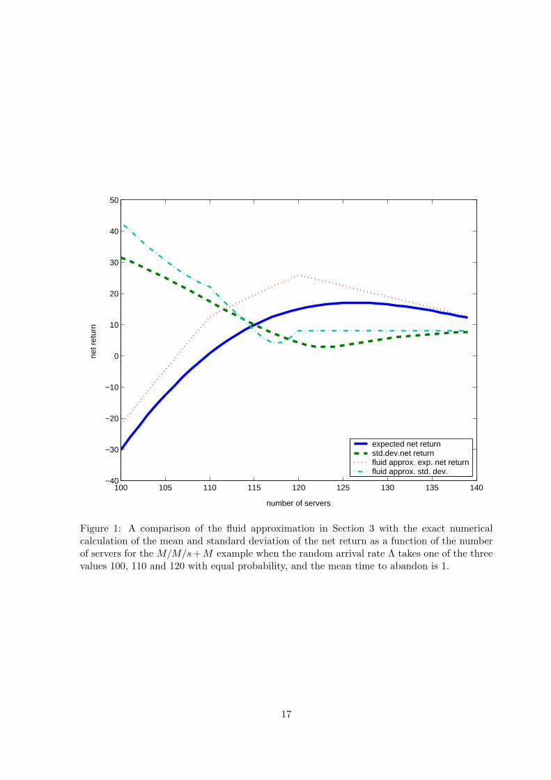
Figure 1: A comparison of the fluid approximation in Section 3 with the exact numericalcalculation of the mean and standard deviation of the net return as a function of the numberof servers for the M/M/s + M example when the random arrival rate Λ takes one of the threevalues 100, 110 and 120 with equal probability, and the mean time to abandon is 1.

17

the number of servers range from 100 to 140. As we should anticipate, the exact expected net

return is a concave function, first increasing in s and then decreasing. In Figure 1 the exact

expected net revenue is maximized at s = 126, yielding the value E[R(126)] = 17.0.

We also see that standard deviation tends to be smaller when the mean is larger, so that

there is not a significant mean-variance tradeoff. The standard deviation is especially large

at lower staffing levels. The standard deviation is minimized at s = 123, yielding the value

SD(R(123)) = 2.86. We achieve high mean return together with a low standard deviation, if

we choose the number of servers appropriately. The expected net return is flatter to the right

of the optimum value than to the left, implying that, in this case, it would be safer to overstaff

than understaff.

Having the standard deviation of the return high (low) where the mean is low (high) is

consistent with intuition: First, low staffing levels will be good if Λ is low, but there will be

serious under-staffing if Λ turns out to be high. On the other hand, high staffing levels will be

good if Λ is high, but there will be serious over-staffing if Λ turns out to be low. We anticipate

that the risk of a mismatch will be reflected by the standard deviation as well as the mean,

and we see that is the case.

Figure 1 shows the quality of the fluid approximation in this case. From Figure 1, we

conclude that the fluid-approximation captures the main effects, but it is not highly accurate.

In this case, the fluid approximation achieves its maximum expected net return at the maximum

possible arrival rate s = 120, as is easy to verify analytically from the simple fluid formulas.

The fluid approximation for the expected net return is also concave, first increasing and then

decreasing.

As we should anticipate, the fluid approximation for the expected net return is an upper

bound on the exact expected value. That will consistently be the case in all our examples.

We have no general proof, but it may be possible to reason as in Jimenez and Koole (2004).

From the perspective of expected net return, the fluid approximation represents the best-

case scenario, where there is no performance degradation due to stochastic-process variability.

When the gap between the fluid approximation and the exact solution is small, we have achieved

almost all possible economies of scale.

Additional insight can be gained by looking at the individual performance measures and

component revenues and costs. To illustrate, we plot the exact values of the component

expected throughput revenue and the individual expected costs, along with the overall expected

net return, as functions of s in Figure 2. We plot the negative values of the three expected

18

100 105 110 115 120 125 130 135 140−40

−30

−20

−10

0

10

20

number of servers

retu

rn

overall expected net returnexp. revenue − 100minus (exp. server cost − 70)minus exp. abandon cost

Figure 2: The component exact expected revenues or negative costs for the first base-caseexample in Figure 1. In this case the expected waiting costs equal the expected abandonmentcosts.

19

costs, so that the expected net return is simply the sum of the other displayed functions.

Since the mean steady-state waiting time equals the product of the mean time to abandon

and the abandonment probability in the M/M/s+M model, the expected abandonment costs

equal the expected waiting costs in this example, where the mean abandonment time is 1

and ca = cw = 2.5. Thus only the expected abandonment cost function appears in Figure 2.

(The expected waiting cost function falls on top of it.) To have the total values of all four

components comparable, we subtract the constant 100 from the expected throughput revenue

and we subtract the constant 70 from the expected server cost. The four components are then

directly comparable.)

From Figure 2, we see that the expected net return is the sum of four concave functions,

three increasing and one decreasing. (Increasing the number of servers is good for throughput,

abandonment and waiting, but bad for server cost.) The assumed costs and revenues guarantee

that there will be an interior maximum for the expected net return.

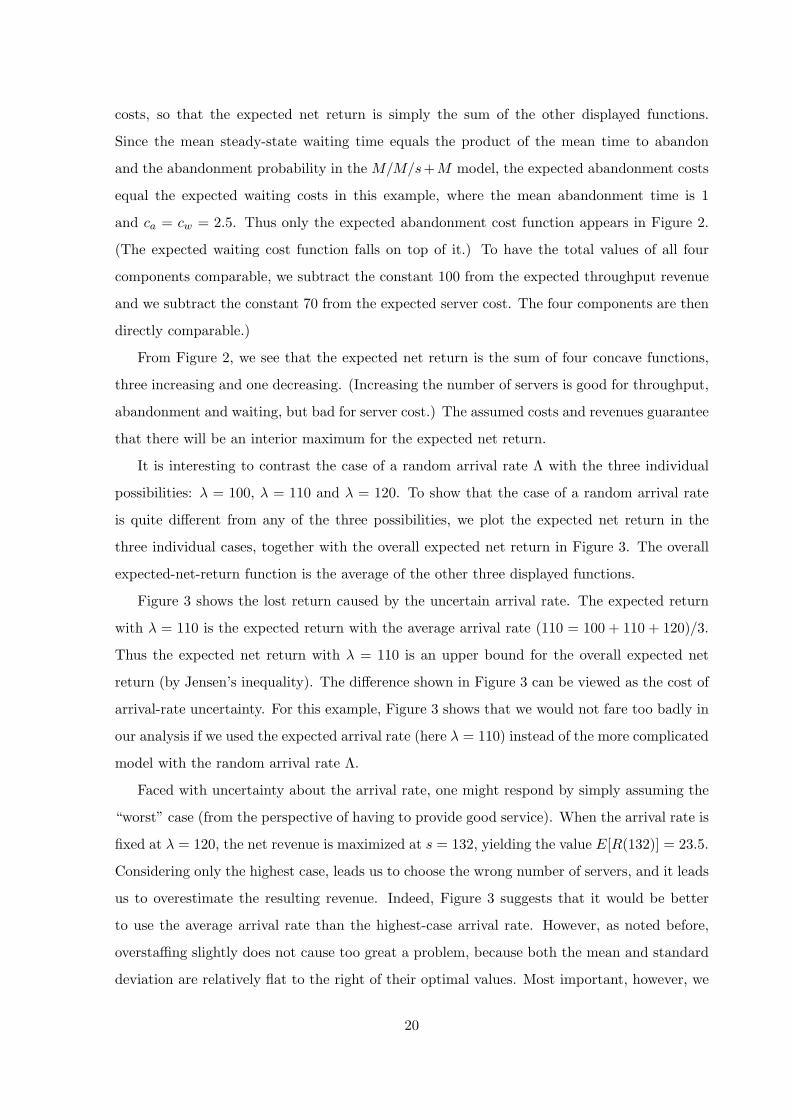
It is interesting to contrast the case of a random arrival rate Λ with the three individual

possibilities: λ = 100, λ = 110 and λ = 120. To show that the case of a random arrival rate

is quite different from any of the three possibilities, we plot the expected net return in the

three individual cases, together with the overall expected net return in Figure 3. The overall

expected-net-return function is the average of the other three displayed functions.

Figure 3 shows the lost return caused by the uncertain arrival rate. The expected return

with λ = 110 is the expected return with the average arrival rate (110 = 100 + 110 + 120)/3.

Thus the expected net return with λ = 110 is an upper bound for the overall expected net

return (by Jensen’s inequality). The difference shown in Figure 3 can be viewed as the cost of

arrival-rate uncertainty. For this example, Figure 3 shows that we would not fare too badly in

our analysis if we used the expected arrival rate (here λ = 110) instead of the more complicated

model with the random arrival rate Λ.

Faced with uncertainty about the arrival rate, one might respond by simply assuming the

“worst” case (from the perspective of having to provide good service). When the arrival rate is

fixed at λ = 120, the net revenue is maximized at s = 132, yielding the value E[R(132)] = 23.5.

Considering only the highest case, leads us to choose the wrong number of servers, and it leads

us to overestimate the resulting revenue. Indeed, Figure 3 suggests that it would be better

to use the average arrival rate than the highest-case arrival rate. However, as noted before,

overstaffing slightly does not cause too great a problem, because both the mean and standard

deviation are relatively flat to the right of their optimal values. Most important, however, we

20

100 105 110 115 120 125 130 135 140−80

−60

−40

−20

0

20

40

number of servers

net r

etur

n

overall exp. net returnlambda = 100lambda = 110lambda = 120

Figure 3: The expected net return as a function of the number of servers in the first M/M/s+Mexample for each of the possible arrival rates: λ = 100, λ = 110 and λ = 120, together withthe overall expected net return.

21

1000 1050 1100 1150 1200 1250 1300 1350 1400−300

−200

−100

0

100

200

300

400

500

number of servers

net r

etur

nexpected net returnstd. dev. net returnfluid approx. exp. net returnfluid approx. std. dev.

Figure 4: A comparison of the fluid approximation in Section 3 with the exact numericalcalculation of the mean and standard deviation of the net return as a function of the numberof servers for the M/M/s+M example with the random arrival rate Λ taking one of the threevalues 1000, 1100 and 1200 with equal probability, when the mean time to abandon is 1.

see that we gain new insight from the full analysis portrayed in Figure 1, beyond what can be

gained from only analyzing the three separate cases λ = 100, λ = 110, and λ = 120.

We now consider variations of the base case. We first consider what happens when the

arrival rates are much larger. To do so, we scale up the base case by multiplying the arrival

rates by 10. In particular, we let the arrival rate assume one of the values 1000, 1100 or 1200,

each with probability 1/3. We again assume that there is no absenteeism, i.e., we let Γ = 1

with probability 1. Again we let the mean time to abandon be 1, just like the mean service

time. We use the same revenue and cost functions. For each of the two methods, we plot the

mean and the standard deviation of the net revenue as a function of the number of servers s in

Figure 4. There is no increased computational complexity to compute the fluid approximation,

but that is not true for the numerical algorithm. It is thus reassuring to see that the numerical

algorithm can handle the scale increase. The run time was a few seconds using matlab.

22

The first thing we see from Figure 4 is the dramatic improvement of the fluid approximation.

When the scale is increased, the fluid model becomes very accurate. Indeed, in this case the

exact numerical solution provides little practical value added in terms of accuracy. Seeing

both results confirms that all economies of scale have been achieved at these high arrival rates.

Figure 4 also shows that the performance is remarkably insensitive to the staffing level at

this scale. Moreover, staffing exactly at s = λmax = 1200, as dictated by the fluid model is

essentially optimal.

In the introduction we contended that the presence of model uncertainty makes it more

appropriate to use a fluid approximation, because the fine model detail should then matter

less. By the same reasoning, the quality of the fluid approximation should improve as the

variability of (Λ, Γ) increases. To illustrate that phenomenon in a simple example, we make

the distribution of Λ in the base case more variable. In particular, we let the three possible

values be 90, 110 and 130 instead of 100, 110 and 120. We thus make the distribution more

variable (in the convex stochastic ordering; see p. 15 of Muller and Stoyan (2002)) while

keeping the mean fixed at 110. The fluid approximation is compared to the exact numerical

algorithm in Figure 5. As expected, we see that the fluid approximation is more accurate than

in the base case in Figure 1. We also see that extra variability lowers the expected return: The

optimal expected net return has been reduced from 17.0 in Figure 1 to 10.4 in Figure 5. The

lost expected return can be attributed to increased model uncertainty. In addition, the overall

standard deviation SD(R(s)) has gone up substantially. The fluid approximation describes it

well too.

We now consider alternative mean times to abandon. To do so, we return to the base case,

where the three possible values of the arrival rate are λ = 100, λ = 110 and λ = 120. In

Figures 6 and 7 we compare the fluid approximation to the exact numerical algorithm when

the mean time to abandon is increased to 4 and decreased to 0.25, respectively. The rest of

the model is the same as in Figure 1.

From Figures 6 and 7, we see that the quality of the fluid approximation improves (degrades)

as the mean time to abandon increases (decreases). The fluid approximation is excellent when

the mean time to abandon is increased to 4, but it is not good when the mean time to abandon

is decreased to 0.25.

23

90 100 110 120 130 140 150−100

−80

−60

−40

−20

0

20

40

60

80

100

number of servers

net r

etur

n

expected net returnstd. dev. net returnfluid approx. exp. net returnfluid approx. std. dev.

Figure 5: A comparison of the fluid approximation in Section 3 with the exact numericalcalculation of the mean and standard deviation of the net return as a function of the numberof servers for the M/M/s+M example with the random arrival rate Λ taking one of the threevalues 90, 110 and 130 with equal probability, when the mean time to abandon is 1.

24

100 105 110 115 120 125 130 135 140−150

−100

−50

0

50

100

150

number of servers

net r

etur

n

expected net returnstd. dev. net returnfluid approx. exp. net returnfluid approx. std. dev.

Figure 6: A comparison of the fluid approximation in Section 3 with the exact numericalcalculation of the mean and standard deviation of the net return as a function of the numberof servers in the M/M/s + M example with the random arrival rate Λ taking one of the threevalues 100, 110 and 120 with equal probability, when the mean time to abandon is increasedto 4.

25

100 105 110 115 120 125 130 135 140−15

−10

−5

0

5

10

15

20

25

30

number of servers

net r

etur

n

expected net returnstd. dev. net returnfluid approx. exp. net returnfluid approx. std. dev.

Figure 7: A comparison of the fluid approximation in Section 3 with the exact numericalcalculation of the mean and standard deviation of the net return as a function of the numberof servers in the M/M/s + M example with the random arrival rate Λ taking one of the threevalues 100, 110 and 120 with equal probability, when the mean time to abandon is decreasedto 0.25.

26

6. A Normally Distributed Arrival Rate

When we consider random arrival rates, especially when we do so without a detailed analysis

of the distribution of Λ, it is natural to let Λ be normally distributed. In doing so, we are

assuming that the standard deviation of Λ is relatively small compared to its mean, so that

negative values would occur with only negligible probability. That seems realistic for most call

centers.

Thus in this section we assume that Λ = N(m,σ2), where N(m,σ2) denotes a normal ran-

dom variable with mean m and variance σ2. (We assume that m > 3σ, so that negative values

can be ignored.) In this section we derive an analytical expression for the fluid approximation

for the expected net return when Λ is normally distributed, Γ = 1 and the revenue and cost

functions are all linear and homogeneous. For simplicity, we again assume that the time-to-

abandon pdf satisfies f(0) > 0. As noted at the end of Section 3, with these assumptions, the

model will have the structure of the single-period newsvendor problem; e.g., see Section 3 of

Porteus (1990).

In general, when Γ = 1, the fluid approximation for the expected revenue and costs can be

expressed as

E[L(s)] = E[(Λ− s)+] = E[Λ− s|Λ > s]P (Λ > s),

E[T (s)] = sP (Λ > s) + E[Λ|Λ ≤ s]P (Λ ≤ s) = E[Λ]− E[L(s)] ,

E[ΛW (s)] = E[L(s)]/f(0) , (6.1)

so, as observed in Section 3, the number of costs and revenues considered can be reduced. We

can then use formulas for conditional normal moments, e.g., see Proposition 18.3 of Browne

and Whitt (1995), to find explicit expressions when Λ = N(m,σ2). For this purpose, let Φ

be the cdf and let φ be the pdf of a standard normal random variable N(0, 1). Let Φc be

the complementary cdf, i.e., Φc(t) = 1 − Φ(t). (The key relations are xφ(x) = −φ′(x) and

x2φ(x) = φ(x) + φ′′(x).) Then,

E[L(s)] = (m− s)Φc((s−m)/σ) + σφ((s−m)/σ) ,

E[T (s)] = m−E[L(s)] . (6.2)

From (3.26), the fluid approximation for the overall expected net return is

E[R(s)] = rtm− (rt + ca + (cw/f(0)))E[L(s)]− css , (6.3)

27

100 110 120 130 140 150 160 170 180−40

−30

−20

−10

0

10

20

30

number of servers

expe

cted

net

ret

urn

variance = 100variance = 200variance = 300variance = 400variance = 500variance = 600

Figure 8: The fluid approximation for the expected net return as a function of the numberof servers and the variance of the arrival rate in the M/M/s + M model when Λ is normallydistributed with mean 110. The six variances range from 100 to 600.

where E[L(s)] is given in (6.2). In this case, from (3.33) we see that the optimal value s∗

satisfies

P (Λ > s∗) = P (N(m,σ2) > s∗) = P (N(0, 1) > (s∗ −m)/σ) =cs

rt + ca + (cw/f(0)). (6.4)

To illustrate, we display the calculated fluid approximation for the expected net return in

the M/M/s + M model when Λ is normally distributed for six cases in Figure 8. We keep

all parameters of the base case in Section 5, except we change the distribution of the random

arrival rate Λ. In all six cases, E[Λ] = 110, as in the base case in Section 5. What changes

from case to case is the variance of Λ. We consider six possible variances: 100, 200, 300, 400,

500 and 600. As we should anticipate, Figure 8 shows that the expected net return decreases

and the optimal number of servers increases as the variance increases. The loss in expected

net return decreases as the variance increases.

28

7. Conclusions

In this paper we introduced a model of a single-class call center with model-parameter

uncertainty. Specifically, we considered the M/GI/s + GI model with uncertainty about

the arrival rate and the number of servers, represented by the random vector (Λ, Γ). We

then developed tools for (i) approximately describing the overall steady-state performance, (ii)

determining near-optimal staffing levels, and (iii) gaining insight into the impact of different

forms of uncertainty. In particular, we focused on the impact on the mean and standard

deviation of the overall net return in the presence of throughput revenue and several costs.

That in turn enabled us to determine near-optimal staffing levels when there is uncertainty

about the arrival rate and the number of servers that will be present.

Our analysis shows that model-parameter uncertainty can make a big difference, but the

effect on staffing was not too great in our examples. In our examples, the expected net return

as a function of the number of servers was relatively flat. But, rather than drawing definitive

conclusions about whether or not model-parameter uncertainty matters, we would emphasize

the approach, which makes it possible to form an independent judgment, and investigate the

impact of different kinds of uncertainty, in other specific scenarios. A similar approach might

be exploited, with the aid of simulation, to study more complex call centers with skill-based

routing.

Our approach here to model-parameter uncertainty has been to compute the overall aver-

age performance, weighting the conditional performance given the model parameters by the

probability of those parameter values. In contrast, call-center managers may want to hedge

against that uncertainty by providing flexibility to change the staffing level upon short notice

in response to unanticipated changes in demand, as discussed in Whitt (1999). The present

analysis can be used to show the advantage of such hedging strategies.

This paper has focused on concepts and numerical examples, not asymptotics. However,

it is significant that heavy-traffic limits justify fluid approximations, showing that they are

asymptotically correct as the scale increases. In particular, a many-server heavy-traffic limit

supporting the fluid approximation used here, without model-parameter uncertainty, is con-

tained in Whitt (2005b) in a discrete-time framework. However, it still remains to establish the

associated fluid limit in the customary continuous-time framework; that remains an important

direction for future research. It is evident, though, that the fluid limit should extend. Those

fluid limits imply corresponding fluid limits when we incorporate model-parameter uncertainty;

29

they directly imply convergence for the integrands in an integral with respect to a fixed mea-

sure (when we average with respect to the distribution of the random vector (Λ, Γ)). Under

regularity conditions, that will imply convergence of the integrals themselves. Consistent with

such a generalized fluid limit, we see that the accuracy of the fluid approximation improves as

scale increases. That phenomenon was illustrated when we compared Figures 1 and 4.

It is also interesting and important that the quality of the fluid approximation in the setting

of model uncertainty improves as the model uncertainty increases. The intuitive explanation is

that the fine detail of the stochastic processes describing the system behavior for given model

parameters become less critical when new variability is introduced in a longer time scale (the

model uncertainty). This phenomenon was illustrated when we compared Figures 1 and 6.

More generally, it suggests that deterministic fluid models should prove to be especially useful

in the setting of model-parameter uncertainty.

8. Acknowledgment.

The author was supported by NSF grant DMI-0457095.

30

References

Altman, E., T. Jimenez, G. Koole. 2001. On the comparison of queueing systems with their

fluid limits. Prob. Eng. Inf. Sci. 15 (2) 165–178.

Avramidis, A. N., A. Deslauriers, P. L’Ecuyer. 2004. Modeling daily arrivals to a telephone

call center. Management Science 50 (7) 896–908.

Baccelli, F., G. Hebuterne. 1981. On queues with impatient customers. In Performance ’81,

ed. F. J. Kylstra, North-Holland, Amsterdam, pp. 159–179.

Bassamboo, A., A. Zeevi, J. M. Harrison. 2006a. Design and control of a large call center:

asymptotic analysis of an LP-based method. Operations Research, forthcoming.

Bassamboo, A., A. Zeevi, J. M. Harrison. 2006b. Dynamic routing and admission control in

high-volume service systems: asymptotic analysis via multi-scale fluid limits. Queueing

Systems, forthcoming.

Ben-Tal, A., A. Nemirovski. 2000. Robust solutions of linear programming problems con-

taminated with uncertain data. Mathmatical Programming 88 (3) 411-424

Borst, S., A. Mandelbaum, M. I. Reiman. 2004. Dimensioning large call centers. Operations

Research 52 (1) 17–34.

Brandt, A., M. Brandt. 1999. On the M(n)/M(n)/s queue with impatient calls. Performance

Evaluation 35 (1) 1–18.

Brandt, A., M. Brandt. 2002. Asymptotic results and a Markovian approximation for the

M(n)/M(n)/s + GI system. Queueing Systems 41 (1-2) 73–94.

Brown, L. D., N. Gans, A. Mandelbaum, A. Sakov, H. Shen, S. Zeltyn, L. Zhao. 2005.

Statistical analysis of a telephone call center: a queueing-science perspective. J. Amer.

Statist. Assoc. 100 (1) 36–50.

Browne, S., W. Whitt, 1995. Piecewise-linear diffusion processes. Advances in Queueing, J.

Dshalalow, ed., CRC Press, Boca Raton, FL, 463–480.

31

Feldman, Z., A. Mandelbaum, W. A. Massey, W. Whitt. 2005. Staffing of time-varying

queues to achieve time-stable performance. Management Science, forthcoming.

Available at http://columbia.edu/∼ww2040.

Gans, N., G. Koole, A. Mandelbaum. 2003. Telephone call centers: tutorial, review and

research prospects. Manufacturing and Service Opns. Mgmt. 5 (2) 79–141.

Garnett, O., A. Mandelbaum, M. I. Reiman. 2002. Designing a call center with impatient

customers. Manufacturing and Service Opns. Mgmt., 4 (3) 208-227.

Green, L., P. Kolesar. 1991. The pointwise stationary approximation for queues with non-

stationary arrivals. Management Science 37 (1) 84–97.

Green, L. V., P. J. Kolesar, W. Whitt. 2005. Coping with time-varying demand when setting

staffing requirements for a service system. Production and Operations Management,

forthcoming. Available at http://columbia.edu/∼ww2040.

Harrison, J. M., A. Zeevi. 2005. A method for staffing large call centers based on stochastic

fluid models. Manufacturing and Service Management, 7 (1) 20–36.

Helton, J. C., D. E. Burmaster. 1996. Treatment of Aleatory and Epistemic Uncertainty,

Special issue of Reliability Engineering and System Safety 54 (2-3) 91–262.

Henderson, S. G. 2003. Input model uncertainty: why do we care and what should we do

about it? Proceedings 2003 Winter Simulation Conference, S. Chick, P. J. Sanchez, D.

Ferrin and D. J. Morrice (eds.), 90–100.

Jennings, O. B., A. Mandelbaum, W. A. Massey, W. Whitt. 1996. Server staffing to meet

time-varying demand. Management Science 42 (10) 1383–1394.

Jimenez, T., G. Koole. 2004. Scaling and comparison of fluid limits of queues applied to call

centers with time-varying parameters. OR Spectrum 26 (3) 413-422.

Jongbloed, G., G. Koole. 2001. Managing uncertainty in call centers using Poisson mixtures.

Applied Stochastic Models in Business and Industry, 17 (4) 307–318.

Mandelbaum, A., W. A. Massey, M. I. Reiman. 1998. Strong approximations for Markovian

service networks. Queueing Systems 30 (1-2) 149–201.

32

Mandelbaum, A., W. A. Massey, M. I. Reiman, R. Rider. 1999. Time-varying multiserver

queues with abandonments and retrials. In Proceedings of the 16th International Tele-

traffic Congress (ITC 16), P. Key and D. Smith (eds.).

Mandelbaum, A., S. Zeltyn. 2004. The impact of customers patience on delay and abandon-

ment: some empirically-driven experiments with the M/M/n + G queue. OR Spectrum

26 (3) 377–411.

Massey, W. A., W. Whitt. 1998. Uniform acceleration expansions for Markov chains with

time-varying rates. Ann. Appl. Prob. 8 (4) 1130–1155.

Muller, A., D. Stoyan. 2002. Comparison Methods for Stochastic Models and Risks, Wiley.

Palm, C. 1943. Intensity Variations in Telephon Traffic, in German, Ericsson Technics 44.

Translated into English, North-Holland, 1988.

Plum, R. R. 1986. History of Traffic Measurement in the Bell System, Dickpat publications,

Red Bank, New Jersey.

Porteus, E. L. 1990. Stochastic inventory theory. Ch. 12 in Stochastic Models, Handbooks in

Operations Research and Management Science 2, D. P. Heyman and M. J. Sobel (eds.),

North-Holland, 605–652.

Ross, A. M. 2001. Queueing Systems with Daily Cycles and Stochastic Demand with Uncertain

Parameters, doctoral dissertation, University of California, Berkeley.

Shen, H., J. Z. Huang. 2005. Analysis of call center data using singular value decomposition.

Applied Stochastic Models in Business and Industry, 21 (3) 251–263.

Steckley, S. G., S. G. Henderson, V. Mehrotra. 2004. Service system planning in the presence

of random arrival rate. working paper, Cornell University.

van Mieghem, J. A. 2003. Capacity management, investment and hedging: review and recent

developments. Manufacturing and Service Management 5 (4) 269–302.

Ward, A. R., P. W. Glynn. 2003. A diffusion approximation for a Markovian queue with

reneging. Queueing Systems, 43 (1-2) 103-128.

Whitt, W. 1991. The pointwise stationary approximation for Mt/Mt/s queues is asymptoti-

cally correct as the rates increase. Management Science 37 (3) 307–314.

33

Whitt, W. 1999. Dynamic Staffing in a Telephone Call Center Aiming to Immediately Answer

All Calls. Operations Research Letters 24 (5) 205–212.

Whitt, W. 2002. Stochastic-Process Limits, Springer, New York.

Whitt, W. 2004. Efficiency-driven heavy-traffic approximations for many-server queues with

abandonments. Management Sci. 50, 1449–1461.

Whitt, W. 2005a. Engineering solution of a basic call-center model. Management Sci. 51 (2)

221–235.

Whitt, W. 2005b. Fluid models for multi-server queues with abandonments. Operations

Research, forthcoming. Available at http://columbia.edu/∼ww2040.

Whitt, W. 2005c. Two fluid approximations for multi-server queues with abandonments.

Operations Research Letters 33 (4) 363–372.

Whitt, W. 2006. Sensitivity of performance in the Erlang A model to changes in the model pa-

rameters. Operations Research, forthcoming. Available at http://columbia.edu/∼ww2040.

Zeltyn S.. A. Mandelbaum. 2005. Call centers with impatient customers: many-server

asymptotics of the M/M/n+G queue.

Available at http://iew3.technion.ac.il/serveng/References.references.html.

Zohar, E., A. Mandelbaum, N. Shimkin. 2002. Adaptive behavior of impatient customers in

tele-queues: theory and empirical support. Management Science 48 (4) 566–583.

34