Staffing a Call Center with Uncertain Non-Stationary

Arrival Rate and Flexibility

Shuangqing Liao1• Ger Koole2 • Christian van Delft3 • Oualid Jouini1

1Laboratoire Genie Industriel, Ecole Centrale Paris, Grande Voie des Vignes, 92290Chatenay-Malabry, France

2Department of Mathematics, VU University Amsterdam, De Boelelaan 1081a, 1081 HVAmsterdam, The Netherlands

3Departement Management des Operations et des Systemes d’Information, Groupe HEC,Rue de la Liberation 78351 Jouy-en-Josas, France.

shuangqing.liao@ecp.fr • koole@few.vu.nl • vandelft@hec.fr • oualid.jouini@ecp.fr

Abstract

We consider a multi-period staffing problem in a single-shift call center. The call

center handles inbound calls, as well as some alternative back-office jobs. The call

arrival process is assumed to follow a doubly non-stationary stochastic process with a

random mean arrival rate. The inbound calls have to be handled as quickly as pos-

sible, while the back-office jobs, such as answering emails, may be delayed to some

extent. The staffing problem is modeled as a generalized newsboy-type model under

an expected cost criterion. Two different solution approaches are considered. First,

by discretization of the underlying probability distribution, we explicitly formulate the

expected cost newsboy-type formulation as a stochastic program. Second, we develop

a robust programming formulation. The characteristics of the two methods and the

associated optimal solutions are illustrated through a numerical study based on real-life

data. In particular we focus on the numerical tractability of each formulation. We also

show that the alternative workload of back-office jobs offers an interesting flexibility

allowing to decrease the total operating cost of the call center.

Keywords: Call centers; uncertain arrival rate parameters; staffing; newsboy model;

stochastic programming; robust programming.

1

1 Introduction

Call centers have become more and more important for many large organizations. For

instance, Brown et al. (2002) report that in 2002 more than 70% of all customer-business

interactions were handled by call centers. They also report that call centers in the U.S.

employ more than 3.5 million people, i.e. 2.6% of the workforce. Due to the importance

of this industry, considerable literature has focused on the operations management of call

centers, in particular on the following issues: demand forecasting, quality of service and

call routing (often using queueing theory), and staffing and agents shift scheduling (using

combinatorial optimization). We refer the reader to the comprehensive surveys of Gans et al.

(2003) and Aksin et al. (2007). In this paper, we consider a call center staffing problem of

a given working day. A central feature in call centers is the significant uncertainty in the

number and length of calls or on the effective number of available agents. This randomness

leads to performance measures which deviate from those predicted at the moment of planning

(see Avramidis et al. (2004); Harrison and Zeevi (2005); Whitt (2006); Robbins (2007) and

Green et al. (2007)).

The staffing cost is a major component in the operating costs of call centers. Unfor-

tunately, uncertainty plaguing the arrival process and the corresponding workloads usually

leads to a complex staffing problem. Traditionally, most call center models in the literature

assume known and constant mean arrival rates, mainly for tractability issues. However, in

addition to the usual uncertainty captured by a stochastic process modeling, real data show

another uncertainty in the process parameters themselves. In this paper, we consider the

staffing problem of a single shift call center, in which we allow the mean arrival rate of calls

to be uncertain. We model the arrival process of calls by a doubly non-stationary stochastic

process, with random mean arrival rates. As in the traditional way, a service level constraint

limits the waiting time for inbound calls. In addition to the job of calls, our call center has to

process back-office jobs, such as answering emails. These additional jobs are assumed to be

given at the beginning of the day and have to be processed within the same day, if necessary

in overtime. We also allow the workload of back-office jobs to be random. The possibility

of delaying back-office jobs introduces some flexibility to the daily workforce management.

A typical example of our call center is that of a hospital, or of a government or of a public

agency, where inbound calls and back-office operations are handled by agents in a single shift

2

(during administrative hours). The agents can be, in real-time, affected to one job type or

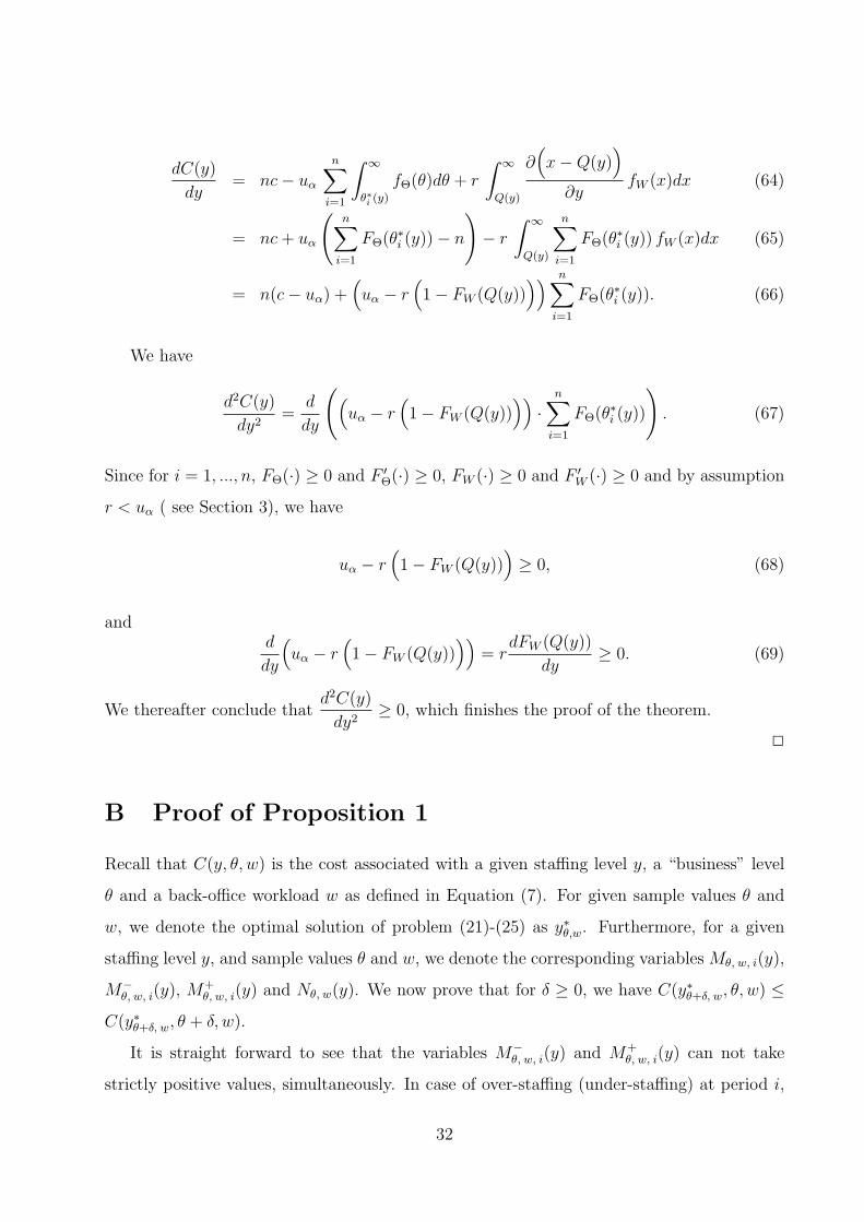
another depending on the actual workload and the operating costs.

As mentioned above, our staffing problem incorporates uncertainty in the call arrival

parameters. The staffing problem is modeled as a cost optimization-based newsboy-type

model. The cost criterion function includes the regular and overtime salary cost and a

penalty cost for excessive waiting times for inbound calls. Our objective is to find the optimal

staffing level which minimizes the total call center operating cost. We consider a multi-period

single-shift call center staffing problem, with the constant staffing level as the single decision

variable. We propose two solution methodologies. First, we formulate the problem as a

stochastic program, by a discretization of the underlying probability distributions. The

second approach relies on robust optimization theory. We prove a convexity result of the

problem, which allows us to find the optimal solution via a relaxed real-valued optimization

model. We then conduct a numerical study in order to illustrate the main characteristics

of the two approaches and the associated optimal solutions. In the numerical illustration,

we use real data gathered from a call center of a Dutch hospital handling inbound calls and

emails.

We distinguish two main contributions in this paper. The first contribution is the mod-

eling and the analysis of the staffing problem of a call center with two types of jobs and

uncertain arrival parameters: inbound calls, to be handled as quickly as possible, and back-

office jobs, that can be delayed to some extent. The second contribution is the analysis of

the impact of the flexibility offered by back-office workloads. We show that combining the

two types of jobs offers flexibility, partially absorbing the undesirable effects of uncertainty

in the arrival parameters.

The rest of the paper is structured as follows. In Section 2, we provide a review of related

literature. In Section 3, we describe the call center model under consideration and formulate

the associated staffing problem. In Section 4, we present the different solution approaches.

In Section 5, we then conduct a numerical study to evaluate these alternative formulations.

We exhibit the impact of the uncertainty of the call arrival parameter and the benefits of

the flexibility offered by back-office workloads on the optimization problem. In Section 6, we

extend the analysis to more general cases, with overflows of calls between successive periods.

The paper ends with concluding remarks and highlights some future research.

3

2 Literature Review

Operations management of call centers constitutes a large stream of research. Many models

in the literature address the key issue of call center staffing and scheduling under stationary

parameters. The considered randomness concerns exclusively the stochastic variability of

inter-arrival and service times. The impact of fluctuations in the arrival rates (and the asso-

ciated flexibility issue) is ignored and the results rely on the assumption of known stationary

arrival rates. However, it has become apparent that general queueing systems performance

indicators are very sensitive to fluctuations of the parameters characterizing the arrival pro-

cess overtime, see for example Ingolfsson et al. (2007). As a consequence, a stream of research

has begun to address the problem of how call centers can better manage the capacity-demand

mismatch that results from arrival rate uncertainty.

First, the pure statistical forecasting issue has been considered in several papers analyzing

the probability distribution of arrival rates (see Avramidis et al. (2004); Brown et al. (2005,

2002); Weinberg et al. (2007); Shen and Huang (2008); Aldor-Noiman et al. (2009)). Various

call center particularities have been pointed out in these studies.

As a second step, the analysis of performance measures of queueing systems with fluc-

tuating arrival rates has appeared. The first setting concerns deterministic non-stationarity,

i.e., some parameters evolve along time according to a known dynamics. A direct method of

accommodating such time-varying parameters consists of numerically solving the complex

queueing models associated to the transient system behavior, see for example Ingolfsson

et al. (2007) and Yoo (1996). Another intuitive means of accommodating changes in the

arrival rate is to consider piecewise stationary measures over successive intervals, while re-

ducing the time length of the intervals over which such stationary measures could be applied.

This is the essence of the point-wise stationary approximation (PSA) used in Green et al.

(2007); Green and Kolesar (1991); Green et al. (2003); Ingolfsson et al. (2007). In a different

setting, a few papers have considered the issue of random non-stationarity in the arrival

process parameters. In Jongbloed and Koole (2001), the authors include arrival parameter

uncertainty via a Poisson mixture model for the arrival process, which permits to model

the overdispersion associated with random arrival rates. They develop a generalization of

the standard Erlang formula-type staffing approaches. In a different vein, in Harrison and

Zeevi (2005); Whitt (2006); Robbins (2007); Steckley et al. (2004), another idea is developed.

4

It can be summarized as estimating performance indices, by first conditioning on the ran-

dom model-parameter vector, and by thereafter unconditioning to get the effective indices.

Most of these methods assume independent intervals. This would lead to inaccurate results

particularly in this case of systems that are overloaded during a certain number of periods.

Stolletz (2008) proposes a new approximation for time-varying queueing systems that can be

overloaded. The approximation is based on the modeling of the overflow of calls between the

periods. Another paper which models dependency between the periods is that of Thompson

(1993). The latter does not however allow the analysis of overloaded systems.

The last issue concerns the call center staffing optimization problem under non-stationary

parameters. Some models rely on a fixed staffing level methodology: there is no possible

flexibility during a daily period and the staffing cannot be updated throughout the day.

In Harrison and Zeevi (2005); Whitt (2006), this problem is solved via a static stochastic

program using a stochastic fluid model approximation. In Jongbloed and Koole (2001), the

standard Erlang formula-type for a fixed staffing approach is generalized through a new

Poisson mixture model for the arrival process.

In many situations, call centers may indeed benefit from flexible staffing, i.e., the ability

to adjust staffing levels (and/or schedules) from one period to another. Such flexibility may

be attained by utilizing temporary operators, in addition to the permanent operators always

available to provide service. The temporary operators may be either supervisors/decision-

makers or other operators who are on call. Another type of flexibility corresponds to the

presence of different shifts for the operators. By combining such shifts, the operator capacity

can be aligned with the time-varying average workload. A last type of flexibility consists of

combining different types of calls, with different admissible delays. Some flexibility exists as

less urgent calls (as e-mails or calls with a possible callback) can be kept in inventory for some

time. Flexible staffing methods coupled with deterministic time-varying arrival rates has

been considered in numerous papers. We refer the reader to Gans et al. (2003); Green et al.

(2007) and the references therein. A stream of research has sought to use a classical rolling

horizon methodology, based on deterministic arrival rate approximations, updated at each

period. In Hur et al. (2004), a case study is presented in which the staffing problem under

uncertain/non-stationary assumption is addressed via recoursing to a rolling horizon decision

process where each step is modeled as a deterministic system. In an alternative research

stream, the arrival rates are formally taken into account in the model. This approach mainly

5

consists of generalizing the well-known fluid approximation models in order to introduce

staffing level updates for the different periods coupled with available arrival rate updated

forecasts. The time horizon is divided into smaller periods and deterministic forecasts for

the customer arrival rates for each period are used to determine the respective staffing levels

(as in Feldman et al. (2008) and Whitt (1999)).

Lastly, Robbins and Harrison (2010) consider a multi-period multiple-class call center

staffing scheduling cost model, with global service constraints. The authors introduce un-

certainty for parameters via a discretization of the underlying parameters probability dis-

tribution, which amounts to a scenario-based approach coupled with large scale multi-stage

stochastic programs to be numerically solved. The approach has also been applied in the

case of a call center with multiple call types in order to investigate the flexibility introduced

by adding a proportion of cross trained workforce (see Robbins et al. (2007, 2008)). Bhan-

dari et al. (2008) formulate, under suitable assumptions for the arrival process and service

time distributions, the multi-periodic staffing problem as a Markov Decision Process with

probabilistic constraints. In Bertsimas and Doan (2010), the authors develop a fluid model

approximation to solve both the staffing and routing problem for large multi-class/multi-pool

call centers with random arrival rates and customer abandonment. The model is solved via

a robust optimization approach. Gurvich et al. (2010) propose a fluid approximation model

for large-scale multi-class call centers with uncertain parameters. The optimal staffing prob-

lems is solved by a chance-constrained programming approach. Helber and Henken (2010)

consider a shift scheduling problem of complex call centers with random arrival rates, skills-

based routing, impatient customers and retrials. These authors propose a specific approach

in which a discrete-time model captures, for a few simulated samples, the dynamics of the

systems due to the time-dependent arrival rates. The associated integer program has then

to be numerically solved.

In this paper, we consider a setting in which there exists some flexibility to modify in real-

time (within the same day) the instantaneous capacity for dealing with inbound calls. The

alternative work for the employees is to handle the day’s workload of back-office jobs. The

flexibility arises from the fact that back-office jobs, which can be viewed as storable, can be

answered at any time of the day, but they have to be treated within the same day, in overtime

if necessary. The inbound calls in our model should be handled (almost) immediately, using

a standard service level constraint (on average at least a given fraction of customers should

6

wait less than a given time). This constraint has to be satisfied on a period-by-period basis.

After closing the inbound calls channel, agents can recourse to work on overtime hours in

order to handle eventual unfinished back-office jobs.

3 Problem Formulation

We consider a multi-period single-shift call center staffing problem. The call center handles

various types of jobs: inbound calls as well as some alternative back-office jobs. The mean

arrival rate of inbound calls is allowed to be uncertain. The workload of the back-office

jobs is also uncertain. The inbound calls have to be handled as soon as possible, while the

back-office jobs, such as emails, can be delayed to some extent within the same day. In this

section, we describe the corresponding stochastic minimal cost staffing problem.

3.1 The Inbound Call Arrival Process

Several characteristics of the arrival process of calls have been underlined in the recent call

center literature. First, it has been observed that the total daily number of calls has an

overdispersion relative to the classical Poisson distribution. Second, the mean arrival rate

considerably varies with the time of day. Third, there is a strong positive correlation between

arrival counts during the different periods of the same day. We refer the reader to Avramidis

et al. (2004) and Brown et al. (2005) for more details.

In order to address uncertain and time-varying mean arrival rates coupled with significant

correlations, we model the inbound call arrival process by a doubly stochastic Poisson process

(see Avramidis et al. (2004); Harrison and Zeevi (2005), and Whitt (1999)) as follows. We

assume that a given working day is divided into n distinct, equal periods of length T , so

that the overall horizon is of length nT . The period length in practice is often 15 or 30

minutes. The mean arrival rate of calls during period i is denoted by Λi and is random. The

stochastic process describing the cumulative number of arrivals up to time t is defined by

A(t) = M(κ∑

i=0

TΛi + (t− Tκ)Λκ+1 : κ = ⌊t/T ⌋), (1)

where M = (M(t) : 0 ≤ t < ∞) is the unit rate Poisson process, and Λ = (Λi : 0 ≤ i ≤ n)

7

is the sequence of arrival rates, with E[n∑

i=1

Λi] < ∞. By conditioning on an outcome of the

average arrival rate in a given period, say λ, the process A(·) is therefore a rate-λ Poisson

process during that period. Furthermore, using the modeling in Avramidis et al. (2004) and

in Whitt (1999), we assume that the arrival rate Λi is of the form

Λi = Θfi, for i = 1, ..., n, (2)

where Θ is a positive real-valued random variable. The random variable Θ can be interpreted

as the unpredictable “busyness” of a day. A large (small) outcome of Θ corresponds to a

busy (not busy) day. The constants fi model the shape of the variation of the arrival rate

intensity across the periods of the day. Formally, if a sample value in a given day of the

random variable Θ is denoted by θ, the corresponding outcome of the arrival rate over period

i for that day is defined by λi = θfi. The random variable Θ is assumed to follow a discrete

probability distribution, defined by the sequence of outcomes θl and the associated sequence

of probabilities pθl , with l = 1, ..., L.

We assume that service times for inbound calls are independent and exponentially dis-

tributed with rate µ. The calls arrive to a single infinite queue working under the the first

come, first served (FCFS) discipline of service. Neither abandonment nor retrials are allowed.

3.2 The Back-Office Workload Process

We assume that the random back-office workload arrives at the beginning of the day. As

an example, one can think of a call center that stores all the emails of a given day and

handles them the next day. We denote by W the number of agents required to handle this

back-office workload during a single period. The random variable W is characterized by a

discrete probability distribution, defined by the sequence of outcomes wk and the associated

sequence of probabilities pwk, with k = 1, ..., K.

3.3 Service Levels and Erlang C Staffing

By only considering inbound calls, our call center can be modeled as an Erlang C model.

We introduce a standard service level constraint for each time period, through which the

waiting time is kept in convenient limits. For period i, let the random variable WTi denote

8

the waiting time of an arbitrary call. The probability distribution of the waiting time of calls

is computed using the classical results of the Erlang C model. In addition to the modeling

assumptions mentioned above, we assume that the mean arrival rates are constant in each

period of the day. This is the point-wise stationary approximation (PSA). We refer the

reader to Green et al. (2003), and Green et al. (2007)) for further details. It is known (see

for example Gross and Harris (1998)) that for a given staffing level v which only handle

inbound calls, one has for period i,

Pr{WTi ≤ AWT | θ}(v) = 1−

(v−1∑m=0

(θ fi/µ)m

m!+

(θ fi/µ)v

v! (1− θ fi/µv

)

)−1

(θ fi/µ)v

v! (1− (θ fi/µ)v

)e−(vµ−θ fi)AWT

= Fθ i(v), (3)

where AWT represents the Acceptable Waiting Time. For a given value of the objective

service level in period i, say SLi%, and a given sample value of the arrival rate, θ fi, this

formula is used in the reciprocal way in order to compute the staffing level which guarantees

the required service level,

vi(θ fi) = F−1θ i (SLi). (4)

3.4 Cost Criterion

In this paper we consider a single-shift call center. Let us denote by y the number of agents

staffed for the day. All the y agents will be therefore present all day long. We also assume

that all agents are able to handle both types of jobs, calls and back-office jobs. We give

priority to inbound calls as follows. For each period i, if the actual number of agents y is

larger than vi(θfi) (the required number of agents to handle the calls), we assign vi(θfi)

agents to calls and y − vi(θfi) agents to back-office jobs. If y < vi(θfi), all the y agents are

assigned to calls. If back-office jobs are not yet finished at the end of the regular working

periods in that day, they are done in overtime.

For a given period, any under-staffing situation is penalized. Under perfectly predictable

arrival rates, a straightforward formulation of the optimization problem is to consider quality-

of-service constraints requiring that the service level SLi is reached in period i. However

in the presence of uncertain arrival rates as in this paper, the service level per period is

9

indeed itself a random variable, depending on the outcomes of the arrival rates. A possible

formulation is to adopt a chance constrained approach requiring that the quality-of-service

constraints are satisfied for some pre-specified fraction of the arrival rate realizations (i.e.

with some given probability). This approach has been used in the context of large skill-based

routing call centers in Gurvich et al. (2010), where the authors have developed a staffing

method leading to nearly optimal solutions.

More clearly, a chance constrained formulation (for a risk level α, and a stochastic pa-

rameter Θ for the arrival process) can be expressed as finding the staffing level yα given

by

Pr{yα ≤ Vi(Θ fi), i = 1, .., n} = α, (5)

with Vi(Θ fi), the underlying random number of agents required to handle the calls in period

i, in order to fulfill the required quality-of-service constraints. By choosing the risk-level α,

the decision-maker may choose a trade-off between staffing costs and “safety” in terms of the

likelihood with which the quality-of-service constraints are met. However, such a formulation

corresponds to quite complex non-convex non-linear optimization problems requiring specific

approximations and heuristics, out of the scope of this paper. In order to propose a solvable

linear programming formulation, the risk level α is expressed via an associated under-staffing

penalty cost denoted as uα. This formulation approach has been applied for example in

Robbins (2007). More concretely for each period i, a proportional under-staffing penalty uα

is paid when the actual capacity y is lower than a sample value of the required agents number

vi(θfi). The value of the parameter uα can be tuned, for example, via an algorithm based on

successive problem solutions and successive numerical estimations of the effective constraint

violation probability α for each current staffing solution. This numerical estimation can

be made through a direct computation if the probability distribution of Θ is known or,

otherwise, through simulations of the arrival process. In the numerical examples presented

in this paper, this tuning procedure algorithm converged very quickly.

In our cost setting, we also assume that each agent gets a salary c per period, the overtime

salary is r per agent per period. As usual, the cost parameters satisfy the ordering c < r < uα

for all possible values of α. The inequality r < uα ensures that inbound calls have the priority

over back-office jobs. The inequality c < r is straightforward.

10

Since the time-horizon of the considered problematic is significant, the cost criterion of

the formulation is the expected daily total cost associated with the staffing level y, which is

expressed as

C(y) = E

[C(y, θ, w)

]=

L∑l=1

K∑k=1

pθl pwkC(y, θl, wk), (6)

with

C(y, θ, w) = n c y + uα

n∑i=1

(y − vi(θfi))− + r

[w −

n∑i=1

(y − vi(θfi))+

]+, (7)

where E[·] denotes the expectation, x+ = max(0, x) and x− = max(0,−x) for x ∈ R. In

Equation (7), the first term is the salary of the agents working during regular time. The

second term is the under-staffing penalty cost. The third is the overtime salary.

Under this economic framework, our objective consists of deciding on the optimal value

of y which minimizes the expected daily total cost given by Equation (6). In the following

theorem we give a convexity result for the expected daily total cost as a function of the

decision variable y. All the proofs of the results in this paper are given in the appendix.

Theorem 1 The expected daily total cost function C(y) is convex in y.

We can see from the proof that no specific assumption on the arrival rates probability

distributions is required.

4 Solution Methodologies

The classical paradigm to solve the problem given by Equation (6) is to develop a determin-

istic approach using the expected values of the random variables Θ and W . The optimal

solution under the deterministic approach might lead to a far greater cost than the actual one

when the parameters take values that are different from those expected, and in particular,

when the system is sensitive to data variation (for example, for a high value of uα). This

will be underlined later in the numerical study. It is thus important to take into account the

effect of data uncertainties and develop better solution approaches.

In this section we develop two different approaches to solve the staffing problem given

by Equation (6), according to the availability of the probability distributions of the random

variables. These approaches are then used in the numerical study in Section 5. First, under

the assumption that the probability distributions associated with the random variables are

11

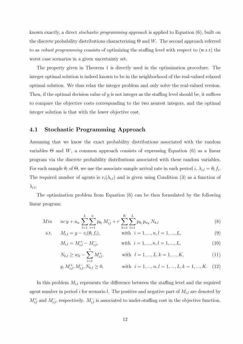
known exactly, a direct stochastic programming approach is applied to Equation (6), built on

the discrete probability distributions characterizing Θ and W . The second approach referred

to as robust programming consists of optimizing the staffing level with respect to (w.r.t) the

worst case scenarios in a given uncertainty set.

The property given in Theorem 1 is directly used in the optimization procedure. The

integer optimal solution is indeed known to be in the neighborhood of the real-valued relaxed

optimal solution. We thus relax the integer problem and only solve the real-valued version.

Then, if the optimal decision value of y is not integer as the staffing level should be, it suffices

to compare the objective costs corresponding to the two nearest integers, and the optimal

integer solution is that with the lower objective cost.

4.1 Stochastic Programming Approach

Assuming that we know the exact probability distributions associated with the random

variables Θ and W , a common approach consists of expressing Equation (6) as a linear

program via the discrete probability distributions associated with these random variables.

For each sample θl of Θ, we use the associate sample arrival rate in each period i, λi,l = θl fi.

The required number of agents is vi(λi,l) and is given using Condition (3) as a function of

λi,l.

The optimization problem from Equation (6) can be then formulated by the following

linear program:

Min nc y + uα

L∑l=1

n∑i=1

pθl M−i,l + r

K∑k=1

L∑l=1

pθl pwkNk,l (8)

s.t. Mi,l = y − vi(θl fi), with i = 1, ..., n, l = 1, ..., L, (9)

Mi,l = M+i,l −M−

i,l, with i = 1, ..., n, l = 1, ..., L, (10)

Nk,l ≥ wk −n∑

i=1

M+i,l, with l = 1, ..., L, k = 1, ..., K, (11)

y,M+i,l,M

−i,l, Nk,l ≥ 0, with i = 1, ..., n, l = 1, ..., L, k = 1, ..., K. (12)

In this problem Mi,l represents the difference between the staffing level and the required

agent number in period i for scenario l. The positive and negative part of Mi,l are denoted by

M+i,l and M−

i,l, respectively. M−i,l is associated to under-staffing cost in the objective function.

12

Nk,l is the over-time workload required in order to finish back-office jobs in scenario (k, l).

This overtime induces overtime cost in the objective function. The unique decision variable

in our staffing problem is the staffing level y.

In this formulation, a possible way to take into account the risk consists of bounding

the conditional-value-at-risk (CVaR), see Rockafellar and Uryasev (2002). Let 0 < β ≤ 1

be a confident level and let CV aRβ be the mean of the total costs belonging to the largest

proportion β. Rockafellar and Uryasev (2002) proved that the minimization of CV aRβ(y)

with respect to the decision variable y is simply given by

miny

CV aRβ(y) = miny,s

{s+ β−1E[(C(y, θ, w)− s)+]}. (13)

Furthermore, the right-hand side of the optimization problem (13) is jointly convex in (y, s)

if the cost function C(y, θ, w) is convex in y.

Ogryczak and Ruszczynski (2002) mention that the CVaR is a coherent risk measure

which is computationally tractable in the framework of stochastic programming. For a given

β, the CVaR optimization problem given by (13) can be formulated by the following linear

program:

Min s+ β−1

K∑k=1

L∑l=1

pwkpθl zk,l (14)

s.t. nc y + uα

n∑i=1

M−i,l + r Nk,l − s ≤ zk,l, with k = 1, ..., K, l = 1, ..., L, (15)

Mi,l = y − vi(θl fi), with i = 1, ..., n, l = 1, ..., L, (16)

Mi,l = M+i,l −M−

i,l, with i = 1, ..., n, l = 1, ..., L, (17)

Nk,l ≥ wk −n∑

i=1

M+i,l, with l = 1, ..., L, k = 1, ..., K, (18)

y,M+i,l,M

−i,l, Nk,l, zk,l ≥ 0, with i = 1, ..., n, l = 1, ..., L, k = 1, ..., K,(19)

s ∈ R. (20)

In Equation (14)-(20) , the variable s represents a critical threshold which is also called

value-at-risk. The variable zk,l represents the positive gap between the total cost in scenario

(k, l) and threshold s. The key point is that this conditional-value-at-risk formulation has

a similar structure as that of the original formulation (8)-(12), i.e., we can again use the

13

real-valued relaxed version in order to solve it.

4.2 Robust Programming Approach

Stochastic programming formulations associated with discrete distributions suffer very often

from the high dimensionality of the corresponding linear programs. We refer the reader to

Thenie et al. (2007) or van Delft and Vial (2004). More importantly, stochastic programming

requires an accurate probabilistic description of the randomness; however, in many life appli-

cations this information is not available. An alternative, non-probabilistic approach can be

implemented via a robust optimization formulation which adopts a Min-Max -type approach

coupled with uncertainty sets associated to the random parameters of the problem. Robust

programming based formulations are often computationally tractable even for large-scale

problems and don’t require a probabilistic description of the uncertain parameters.

A main issue of the robust programming implementation is the design of an efficient

uncertainty set which fixes the trade-off between robustness (i.e., protection against the

worst case) and average performance (see Bertsimas and Brown (2009) and Natarajan et al.

(2009) for further details). If we choose an uncertainty set covering the whole underlying

sample space associated with the random parameters, implemented over sample data, this

solution exhibits the best possible worst case performance, but does poorly on average (see

Soyster (1973)). One can then choose an uncertainty set which does not cover the whole

underlying sample space. In this case, the solution can be expected to exhibit improved

average costs for sample data, however this solution will be less robust to the worst case,

as some of the sample scenarios are likely to be outside of the reduced uncertainty set. By

considering different sizes for the uncertainty sets, one reviews different possible trade-offs

between average performance and protection against uncertainty (see Bertsimas and Sim

(2004)).

We consider a robust approach associated with uncertainty sets for Θ and W . In order

to analyze the above robust formulation, we first study the properties of the optimal value,

denoted as C∗(θ, w), of the purely deterministic optimization problem for given outcomes θ

14

and w,

Min nc y + uα

n∑i=1

M−i + r N (21)

s.t. Mi = y − vi(θ fi), with i = 1, ..., n, (22)

Mi = M+i −M−

i , with i = 1, ..., n, (23)

N ≥ w −n∑

i=1

M+i , (24)

y,M+i ,M

−i , N ≥ 0, with i = 1, ..., n. (25)

In this formulation, Mi represents the difference between the staffing level and the required

agent number in period i. The positive and negative part of Mi are denoted by M+i and

M−i , respectively. M

−i is associated to under-staffing cost in the objective function. N is the

over-time workload required in order to finish back-office jobs.

In the next proposition, we exhibit some properties of C∗(·, ·), that are used in the robust

programming formulation.

Proposition 1 Let C∗(θ, w) be the optimal objective value of the problem defined in (21)-

(25). For δ > 0, we have the following inequalities,

C∗(θ + δ, w) ≥ C∗(θ, w), (26)

C∗(θ, w + δ) ≥ C∗(θ, w). (27)

Proof: See Appendix B.

Corollary 1 For uncertainty sets defined as

U = {(θ, w) : 0 ≤ θ ≤ θ + η σθ, 0 ≤ w ≤ w + η σw, η ≥ 0}, (28)

by Proposition 1, we have

max(θ,w)∈U

C∗(θ, w) = C∗(θ + η σθ, w + η σw). (29)

These results are straightforward by applying Proposition 1 and are intuitively clear: a call

center with additional workload (of calls and/or back-office jobs) will require an additional

cost, related to additional salary, additional under-staffing or overtime costs. The robust

15

formulation of the staffing problem with the uncertainty set (28) is as follows:

Min nc y + uα

n∑i=1

M−i + r N (30)

s.t. Mi = y − vi((θ + η σθ)fi), with i = 1, ..., n, (31)

Mi = M+i −M−

i , with i = 1, ..., n, (32)

N ≥ w + η σw −n∑

i=1

M+i , (33)

y,M+i ,M

−i , N ≥ 0, with i = 1, ..., n. (34)

As in Section 4.1, we relax integrity constraints for the variables. The parameter η ∈ R+

fixes the upper bound values for the uncertain parameters Θ and W in (28). The decision-

maker chooses to fix the trade-off between the protection level against uncertainty and the

average cost performance. We note here that it is also possible to build a formulation mixing

stochastic and robust programming, for example by defining an uncertainty set for Θ and a

probability distribution for W (the corresponding formulation is given in Appendix C).

5 Numerical Comparison

In this section, we conduct a numerical study in order to evaluate the proposed approaches.

In Section 5.1, we describe the numerical experiments. In Section 5.2, we analyze the results

and give some insights.

5.1 Experiments

We first describe the data used in the numerical examples. We next describe the experiments

and give the numerical results.

5.1.1 Parameter Values

Inbound calls. In the experiments we use real data from a Dutch hospital which exhibits a

typical and significant workload time-of-day seasonality. Figure 1 displays the mean arrival

rates as a function of the periods in the day. We focus on a particular day, namely Monday.

With the solid line, we plot this curve for an average day, and in dashed lines we represent two

16

samples corresponding to busy and not busy days. The mean arrival rate at the beginning

and at the end of the day is quite low, exhibits a high peak in the late morning, tends

to decrease around the lunch break, and finally has a second lower peak in the afternoon.

Although there is a significant stochastic variability in the arrival rate from one day to

another, there is a strong seasonal pattern across the periods of a given day. The day starts

at 7 am, finishes at 6 pm, and is divided into n = 11 periods, of one hour each.

Without loss of generality, we choose E[Θ] = 1. This leads to fi = E[Λi], and from a

one-year-horizon data we numerically find via a standard statistical analysis, that f1, f2, ...,

f11 are 3.5, 18.4, 34.4, 31.5, 29.0, 12.9, 28.4, 25.0, 17.4, 7.2, 5.3 calls per minute, respectively.

0

10

20

30

40

50

60

1 2 3 4 5 6 7 8 9 10 11

Period

Arrival rate average day

busy day

not busy day

Figure 1: Solid line: average day; higher dashed line: a busy day; lower dashed line: a notbusy day

Recall that the random variable Θ describes the “business” of the day. We assume that

Θ follows a discretized truncated Gaussian probability distribution. Since we normalized the

realizations of Θ such that E[Θ] = 1, the “business factor”, say θt, of a given day t with a

total daily call number, say Dt, is θt =Dt∑ni=1 fi

. Collecting the θt values of all the days of the

data, we obtain a sequence of values for which we compute a statistical standard deviation.

We find σΘ = 0.21. This finishes the characterization of the random variable Λi.

The mean service time is1

µ= 5 minutes. We assume a classical service level correspond-

ing to the well-known 80/20 rule: the probability that a call waits for less than 20 seconds

has to be larger or equal to 80 percent. Using Condition (3), we can therefore deduce the

17

required number of agents vi during period i.

Back-office jobs. In this real-life case, the back-office jobs correspond to the emails to be

answered in a given day. The random daily workload of emails, W , is assumed to follow

a truncated Gaussian distribution. We consider three scenarios with high, medium and

low workload of emails, corresponding to 1000, 600, 50 for the means and 100, 60, 5 for the

standard deviations, respectively.

Cost parameters. The salary during the regular time is c = 15 per agent per period. The

salary during the overtime is r = 20 per agent per period. For each period, a penalty uα,

for being under-staffed by one agent, is incurred, within the ordering c < r < uα, given

in Section 3.4. We considered three scenarios for the under-staffing probability α = 10%,

α = 5%, α = 1%, and determined, as explained in Section 3.4, the corresponding values for

the penalty cost u10%, u5% and u1%. It should be mentioned that uα depends not only on α,

but also on other parameters of the call center.

5.1.2 Design of the Experiments

Benchmark. As an initial benchmark, we consider the simple approach based on the

expected value of the random variable Θ, referred to as average based deterministic approx-

imation, denoted by DA. In this case, Λi reduces to the single value E[Θ]fi. The required

number of agents to handle the calls of period i is vi(E[Θ]fi) given by Condition (3). Here

we keep the amount of emails W as a random variable, and average on all of its outcomes.

The optimization problem can be then formulated as:

Min nc y + uα

n∑i=1

M−i + r

K∑k=1

pwkNk (35)

s.t. Mi = y − vi(E[Θ] fi), with i = 1, ..., n, (36)

Mi = M+i −M−

i , with i = 1, ..., n, (37)

Nk ≥ wk −n∑

i=1

M+i , with k = 1, ..., K, (38)

y,M+i ,M

−i , Nk ≥ 0, with i = 1, ..., n. (39)

In this problem, Mi represents the difference between the staffing level and the required

agent number in period i for the average arrival rate E[Θ] fi. The positive and negative part

of Mi are denoted by M+i and M−

i . Nk is the over-time workload required in order to finish

18

back-office jobs in scenario k.

Lower bound. As a lower bound solution, we consider a perfect information model (PI )

for which the value of the pair (θ, w), the actual workload, is assumed to be known before

the optimization step of the variable y. For each pair (θl, wk), we solve the problem (40)-(44)

in order to get the optimal value of yl,k and its associated total cost.

Min nc yl,k + uα

n∑i=1

M−i,l + r Nk,l (40)

s.t. Mi,l = yl,k − vi(θl fi), with i = 1, ..., n, l = 1, ..., L, k = 1, ..., K, (41)

Mi,l = M+i,l −M−

i,l, with i = 1, ..., n, l = 1, ..., L, (42)

Nk,l ≥ wk −n∑

i=1

M+i,l, with l = 1, ..., L, k = 1, ..., K, (43)

yl,k,M+i,l,M

−i,l, Nk,l ≥ 0, with i = 1, ..., n, l = 1, ..., L, k = 1, ..., K. (44)

The computation of the corresponding average total cost is then straightforward according

to (6).

Additional Notations. We compute the optimal staffing levels given by the average based

deterministic approximation (DA), the classical stochastic programming approach (SP), ro-

bust (RP) and mixed (MxRP) programming approaches with various robustness levels. For

the robust programming approaches and the mixed robust programming approaches, the

size of the uncertainty sets varies according to η = 0.1, 0.5, 1.0, 2.0 and 3.0.

Optimal policy performance simulations. In order to estimate the cost criterion prob-

ability distribution associated with the different policies, 20000 sample values are randomly

generated as outcomes of (Θ,W ).

5.1.3 Numerical Results

The results are given in Tables 1, 3 and 4, which correspond to low, medium and high

volumes of emails, respectively. Tables 3 and 4 are given in Appendix D. For the value

of uα corresponding to a given estimated under-staffed probability (α = 10%, 5%, 1%) in

the call center, and for a given approach, each table displays the optimal staffing level, the

average total cost, the average values of the three components of the total cost, the standard

deviations (STD.) of the total cost and the under-staffing cost and the over-time cost. At

the end of each line, the under-staffing probability is given.

19

The computations have been performed using Cplex on an Intel Core Duo CPU 1.20 Ghz

with 0.99 GBytes RAM. For the considered problems, the computing time of DA and RP

never exceeded 0.1 seconds while for SP, this time is around 170 seconds.

5.2 Insights

In this section, we comment on the numerical results and derive the main insights. First, we

compare the proposed approaches and show the advantage of explicitly taking into account

the uncertainty in the call arrival parameters. Second, we analyze the benefits of the flex-

ibility provided by emails on our staffing optimization problem and the number of flexible

servers necessary.

5.2.1 Analysis of the numerical experiments

In what follows, we compare between the performance measures of the proposed approaches.

First, we mention that some trade-off exists between the average cost and the associated

standard deviation: Above the threshold which is the optimal staffing level of SP, the average

total cost increases (see Theorem 1) while the associated standard deviation decreases in y.

It is also obvious to see that the under-staffing probability decreases in the under-staffing

penalty uα. For large values of uα, this probability becomes negligible. For the call centers

with the same parameters as those in Tables 1, 3 and 4, we have conducted additional runs

showing that when uα = 1e + 5, the associated under-staffing probabilities are lower than

0.015%.

Concerning the average cost, SP is as expected the most efficient. In Tables 1, 3 and 4, we

observe that for a given value of the risk level α, the optimal solutions of SP of the three tables

are the same. This stems from the fact that for a call center with given distributions of the

“business factor” Θ and the back-office workload W , we associate an under-staffing penalty

cost uα which expresses the chance constraint (5). For a given period i, the distribution of the

required number of agents Vi(Θ fi) is unchanged for the three tables, since the distribution of

Θ is kept the same. Thus, the optimal staffing level y is also unchanged for the three tables.

Note also that the value of the under-staffing penalty cost uα varies with different sizes of

the email workload W . We should mention that if we do not relate the chance constraint (5)

with the under-staffing penalty cost, the optimal staffing level would change with the size of

20

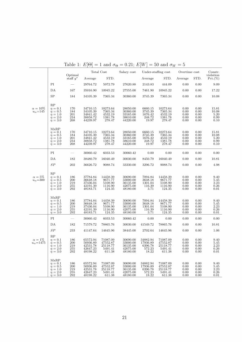
Table 1: E[Θ] = 1 and σΘ = 0.21; E[W ] = 50 and σW = 5

Total Cost Salary cost Under-staffing cost Overtime cost Constr.Optimal violationstaff y∗ Average STD. Average STD. Average STD. Pct.(%)

PI — 29764.72 5972.79 27620.88 2143.83 444.09 0.00 0.00 9.09

DA 167 35016.90 10945.22 27555.00 7461.90 10945.22 0.00 0.00 17.22

SP 184 34105.39 7365.34 30360.00 3745.39 7365.34 0.00 0.00 10.08

RPα = 10% η = 0.1 170 34710.15 10273.64 28050.00 6660.15 10273.64 0.00 0.00 15.81uα=145 η = 0.5 184 34105.39 7365.34 30360.00 3745.39 7365.34 0.00 0.00 10.08

η = 1.0 201 34841.42 4532.19 33165.00 1676.42 4532.19 0.00 0.00 5.20η = 2.0 234 38858.72 1381.78 38610.00 248.72 1381.78 0.00 0.00 0.99η = 3.0 268 44239.97 278.47 44220.00 19.97 278.47 0.00 0.00 0.10

MxRPη = 0.1 170 34710.15 10273.64 28050.00 6660.15 10273.64 0.00 0.00 15.81η = 0.5 184 34105.39 7365.34 30360.00 3745.39 7365.34 0.00 0.00 10.08η = 1.0 201 34841.42 4532.19 33165.00 1676.42 4532.19 0.00 0.00 5.20η = 2.0 234 38858.72 1381.78 38610.00 248.72 1381.78 0.00 0.00 0.99η = 3.0 268 44239.97 278.47 44220.00 19.97 278.47 0.00 0.00 0.10

PI — 30060.42 6033.53 30060.42 0.00 0.00 0.00 0.00 0.00

DA 182 38480.79 16040.49 30030.00 8450.79 16040.49 0.00 0.00 10.81

SP 202 36626.72 9088.74 33330.00 3296.72 9088.74 0.00 0.00 4.98

RPα = 5% η = 0.1 186 37784.84 14458.39 30690.00 7094.84 14458.39 0.00 0.00 9.40uα=300 η = 0.5 200 36648.18 9671.77 33000.00 3648.18 9671.77 0.00 0.00 5.45

η = 1.0 219 37436.04 5108.90 36135.00 1301.04 5108.90 0.00 0.00 2.23η = 2.0 255 42191.39 1116.90 42075.00 116.39 1116.90 0.00 0.00 0.26η = 3.0 292 48183.71 124.35 48180.00 3.71 124.35 0.00 0.00 0.01

MxRPη = 0.1 186 37784.84 14458.39 30690.00 7094.84 14458.39 0.00 0.00 9.40η = 0.5 200 36648.18 9671.77 33000.00 3648.18 9671.77 0.00 0.00 5.45η = 1.0 219 37436.04 5108.90 36135.00 1301.04 5108.90 0.00 0.00 2.23η = 2.0 255 42191.39 1116.90 42075.00 116.39 1116.90 0.00 0.00 0.26η = 3.0 292 48183.71 124.35 48180.00 3.71 124.35 0.00 0.00 0.01

PI — 30060.42 6033.53 30060.42 0.00 0.00 0.00 0.00 0.00

DA 182 71579.72 78865.76 30030.00 41549.72 78865.76 0.00 0.00 10.81

SP 233 41147.64 14645.96 38445.00 2702.64 14645.96 0.00 0.00 1.06

RPα = 1% η = 0.1 186 65572.94 71087.09 30690.00 34882.94 71087.09 0.00 0.00 9.40uα=1475 η = 0.5 200 50936.89 47552.87 33000.00 17936.89 47552.87 0.00 0.00 5.45

η = 1.0 219 42531.78 25118.77 36135.00 6396.78 25118.77 0.00 0.00 2.23η = 2.0 255 42647.23 5491.41 42075.00 572.23 5491.41 0.00 0.00 0.26η = 3.0 292 48198.22 611.38 48180.00 18.22 611.38 0.00 0.00 0.01

MxRPη = 0.1 186 65572.94 71087.09 30690.00 34882.94 71087.09 0.00 0.00 9.40η = 0.5 200 50936.89 47552.87 33000.00 17936.89 47552.87 0.00 0.00 5.45η = 1.0 219 42531.78 25118.77 36135.00 6396.78 25118.77 0.00 0.00 2.23η = 2.0 255 42647.23 5491.41 42075.00 572.23 5491.41 0.00 0.00 0.26η = 3.0 292 48198.22 611.38 48180.00 18.22 611.38 0.00 0.00 0.01

21

back-office workload for fixed under-staffing penalty cost (more details are given in Section

5.2.2).

The gap between the optimal staffing levels of DA and SP is remarkable, especially when

the back-office workload is small. Neither DA captures the negative impact of the randomness

in call arrival rates on service quality, nor on the under-staffing cost. Particularly, it can be

seen that the optimal solutions of DA remains constant once the penalty cost uα exceeds

some threshold. Consequently, in the case of a high penalty cost and significant arrival rate

randomness, DA should not be used. However, it can be noticed that when the back-office

workload is high, the induced flexibility is quite profitable and the global performance of the

DA optimal solution is in that case less affected by the randomness of the arrival process.

As described in Section 4.2, robust optimization relies on a worst-case-type analysis

for a given uncertainty set. In order to examine different trade-offs between the average

performance and the protection against risk, we have considered different η values. The

higher the η value, the higher the degree of protection in the solution. An extreme case

can be considered, namely η = 0, which can be viewed as equivalent to DA. By increasing

the η value, the optimal RP solution includes a progressively increasing over-staffing, which

eliminates under-staffing penalty costs, but at the same time increases the direct salary

costs. Since RP always considers a “worst-case” setting, it is therefore important to choose

an appropriate uncertainty set by taking into account the calls arrival rate variations, the

target α and the flexibility offered by the back-office workload.

In Tables 1 and 3, MxRP has the same optimal solution and cost performance as RP.

Basically, this stems from the fact that the back-office workload uncertainty is not significant

w.r.t. the arrival process randomness. The results exhibit a slight difference for increased

back-office workload uncertainty (see Table 4).

5.2.2 Benefits of The Flexibility Offered by Back-Office Jobs

An obvious benefit from adding back-office jobs comes from the fluctuating shape exhibited

by the call arrival rate as a function of the periods of the days (see Figure 1). Since we

are considering a single shift call center, the strongest quality-of-service constraints (corre-

sponding to the period with the highest arrival rates), tend to force to have a typically high

staffing level for the whole day. Such a level is in fact required for only some periods. Clearly,

22

this situation leads to over-staffing during the other periods, which can be used without any

additional cost in order to handle some back-office jobs. For example, it can be seen from

Tables 1 and 3, that the optimal staffing levels are identical (and do not increase) while the

back-office workload has been increased from 50 to 600. The savings are thus the direct

salary costs corresponding to this increase (namely 600× c = 9000) minus the under-staffing

cost increase and minus the overtime cost increase (which are negligible w.r.t. 9000).

We note also that the variability of the calls arrival process can be smoothed by increasing

back-office workload. Via Tables 1 and 4, it can be observed that for a given risk level α,

the associated uα in the former (with low back-office workload) is greater than that in the

latter (with high back-office workload).

In order to characterize the limits of the flexibility offered by back-office jobs, we analyze

the gain function G(w) associated with the flexibility offered by the back-office workload w.

This function is defined as follows. Denote a given value of under-staffing penalty cost by u,

for sample values θ and w, recall that the optimal total cost for the call center including the

back-office jobs (see Equation (7)) is given by

C(y∗, θ, w) = n c y∗ + u

n∑i=1

(y∗ − vi(θfi))− + r

[w −

n∑i=1

(y∗ − vi(θfi))+

]+, (45)

with y∗ the optimal solution of

miny∈N

{n c y + uE[n∑

i=1

(y − Vi(Θfi))−] + r E[W − E[

n∑i=1

(y − Vi(Θfi))+] ]+}. (46)

If the back-office workload is considered to be externally processed, for a direct cost cw, the

optimal total cost for the call center without any back-office jobs is given by

C ′(y′∗, θ) = n c y′∗ + un∑

i=1

(y′∗ − vi(θfi))−, (47)

where y′∗ is the optimal solution of

miny′∈N

{n c y′ + uE[n∑

i=1

(y′ − Vi(Θfi))−]}. (48)

23

The gain function G(w) may be therefore written as

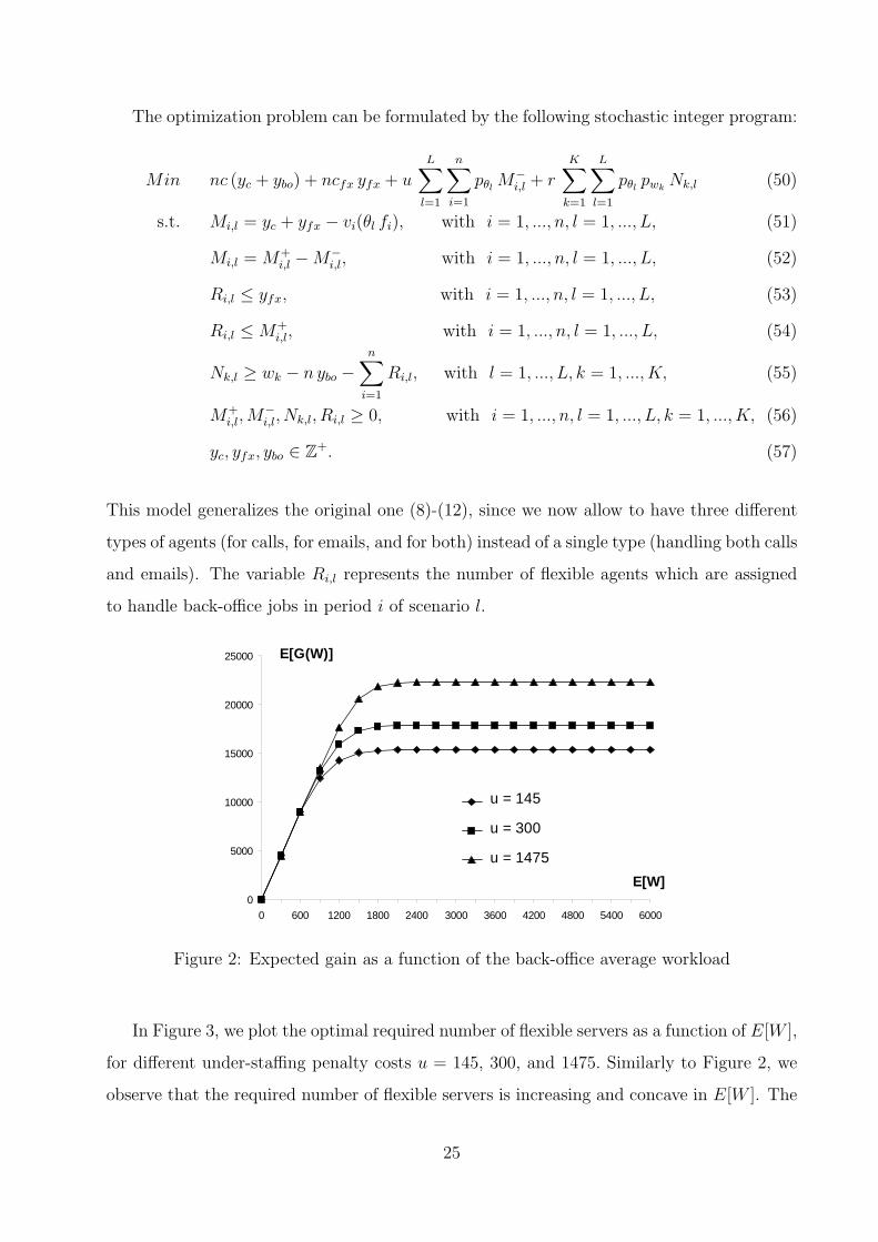
G(w) = C ′(y′∗, θ) + cw − C(y∗, θ, w). (49)

If one considers an SP solving methodology, the corresponding expected profit E[G(W )],

given as a function of the expected value of W , is displayed in Figure 2 for different penalty

cost values u = 145, 300, and 1475. The other parameters are identical to those used in

Section 5.1.

Figure 2 shows that E[G(W )] is an increasing concave function of E[W ], asymptotically

converging towards a constant level for high E[W ] values. We see that above a certain

amount, additional back-office jobs no longer generate an additional profit. Here the thresh-

olds are 2400, 2700 and 3000 for penalty costs respectively given by u = 145, 300 and 1475.

This observation brings forth consideration of the best setting up of the agents groups:

the required number of flexible servers (those able to deal with both calls and back-office

jobs), and that of the specialized servers. With similar parameters as in Section 3, we propose

a model with three types of servers: single skilled servers (for calls), single skilled servers

(for back-office jobs) and flexible servers. The sizes of the three groups are denoted by yc,

ybo, yfx respectively. In order to force the optimal solution to have a minimum number of

flexible servers, while keeping unchanged the total number of servers comparing to the single

type (flexible) servers model analyzed above, the flexible servers’ salary, say cfx, is assumed

to be just slightly increased, w.r.t. the salary of single skilled servers. For our numerical

example, we choose c = 15, and cfx = 15.0001.

24

The optimization problem can be formulated by the following stochastic integer program:

Min nc (yc + ybo) + ncfx yfx + uL∑l=1

n∑i=1

pθl M−i,l + r

K∑k=1

L∑l=1

pθl pwkNk,l (50)

s.t. Mi,l = yc + yfx − vi(θl fi), with i = 1, ..., n, l = 1, ..., L, (51)

Mi,l = M+i,l −M−

i,l, with i = 1, ..., n, l = 1, ..., L, (52)

Ri,l ≤ yfx, with i = 1, ..., n, l = 1, ..., L, (53)

Ri,l ≤ M+i,l, with i = 1, ..., n, l = 1, ..., L, (54)

Nk,l ≥ wk − n ybo −n∑

i=1

Ri,l, with l = 1, ..., L, k = 1, ..., K, (55)

M+i,l,M

−i,l, Nk,l, Ri,l ≥ 0, with i = 1, ..., n, l = 1, ..., L, k = 1, ..., K, (56)

yc, yfx, ybo ∈ Z+. (57)

This model generalizes the original one (8)-(12), since we now allow to have three different

types of agents (for calls, for emails, and for both) instead of a single type (handling both calls

and emails). The variable Ri,l represents the number of flexible agents which are assigned

to handle back-office jobs in period i of scenario l.

0

5000

10000

15000

20000

25000

0 600 1200 1800 2400 3000 3600 4200 4800 5400 6000

E[W]

E[G(W)]

u =145

u =300

u=1475

u = 145

u = 300

u = 1475

Figure 2: Expected gain as a function of the back-office average workload

In Figure 3, we plot the optimal required number of flexible servers as a function of E[W ],

for different under-staffing penalty costs u = 145, 300, and 1475. Similarly to Figure 2, we

observe that the required number of flexible servers is increasing and concave in E[W ]. The

25

0

50

100

150

200

250

300

350

400

0 600 1200 1800 2400 3000 3600 4200 4800 5400 6000

E[W]

u_0.1=145

u_0.05=300

u_0.01=1475

u = 145

u = 300

u = 1475

Number of flexible servers

Figure 3: Required number of flexible servers

0

0,1

0,2

0,3

0,4

0,5

0,6

0,7

0,8

0,9

1

0 600 1200 1800 2400 3000 3600 4200 4800 5400 6000

145

300

1475

u = 145

u = 300

u = 1475

Percentage of flexible servers

E[W]

Figure 4: Percentage of flexible servers over the total number of servers

26

maximum required numbers of flexible servers are 320, 326 and 339 for u = 145, 300 and

1475, respectively. Call center flexibility results from the ability of the flexible servers to deal

with the two types of jobs. In Figure 4, we plot the percentage of flexible servers from the

total number of servers as a function of E[W ], for u = 145, 300, and 1475. Figure 4 shows

that this percentage decreases after a peak around 90%. The reason is that for a given value

of u, the total staffing level increases along with the back-office workload. However, above

a certain amount of back-office workload, the required number of flexible servers remains

constant. The ratio of flexible servers will therefore decrease.

0

5000

10000

15000

20000

25000

0 600 1200 1800 2400 3000 3600 4200 4800 5400 6000

E[W]

E[G(W)] f_i,N(1,0.21)

f'_i,N(1,0.21)

f_i ,N(1,0.1)

f i , N(1,0.21)f i ', N(1,0.21)f i , N(1,0.1)

Figure 5: Expected gain for different seasonal pattern and business variance

15000

16000

17000

18000

19000

20000

1200 1800 2400 3000 3600 4200 4800 5400 6000

E[W]

E[G(W)]

f i +3f i

f i - 3

Figure 6: Expected gain for different call center size

27

The impact of the flexibility on costs performance depends also on the value of the

under-staffing penalty cost and the variability of inbound calls. For small workloads of

back-office jobs, Figure 2 shows that the gains associated with the flexibility are constant

w.r.t. u. Indeed, in such situations, the over-staffed agents (for calls) can easily handle the

back-office jobs without any additional cost. For large back-office workloads and high under-

staffing penalty cost, the gain is larger because a higher staffing level is required, inducing

more over-staffing. The next examples, illustrated by Figures 5 and 6, show the impact of

variability of inbound calls on the gain associated with the flexibility offered by back-office

jobs. This inbound calls variability results from the combination of the variations of the

daily deterministic pattern (defined by the variations of the fi coefficients), of the Θ random

variability and of the inbound calls total average workload (defined by∑n

i=1 fi), that can be

viewed as the call center size.

In Figure 5, we compare three cases. First, the original case is depicted, corresponding

to the daily pattern fi and the random variable Θ with a Gaussian distribution (with mean

equal to 1 and standard deviation equal to 0.21). The two other cases have smoother calls

workload fluctuations, but still the same global daily workload. For one example, we keep

the variability of the process Θ similar, but we smooth the daily pattern by fixing f ′1, f

′2, ...,

f ′11 equal to 13.5, 18.4, 24.4, 21.5, 19, 22.9, 18.4, 25, 17.4, 17.2 and 15.3 calls per minute. It

is worth noting that∑11

i=1 fi =∑11

i=1 f′i . In the second case, the standard deviation of the Θ

random variable is decreased, from 0.21 to 0.10, but the the daily pattern is still given by

the fi parameters. As expected, it can be seen in Figure 5 that the benefit obtained through

flexibility decreases when overall variability decreases, either because of a smoother seasonal

pattern, or because of a reduction of the daily business variance.

In Figure 6, we compare three cases with similar successive periodic daily fluctuations

(i.e. with similar values for the differences fi+1 − fi) and similar Θ process. However, we

vary the inbound calls total average workload (defined by∑n

i=1 fi), which can be viewed

as varying the call center size. We have considered coefficients respectively given by the

sequences fi +3, fi and fi − 3. The figure shows a decrease in the gain obtained from server

flexibility for call center with reduced size. The underlying reason is simple: the size of the

stochastic fluctuations due to Θ is reduced, for smaller fi coefficients, and, as a consequence,

the required (or useful) flexibility level is also smaller.

28

6 Extension to Models with Overflow

In this section, we extend the analysis to call centers with possible call overflows between

successive periods. Some call center models which include an overflow process have been

analyzed in the literature (see Thompson (1993) and Stolletz (2008)). According to these

papers, we assume the outcome of the arrival rate λi, in period i, to be substituted by a

modified auxiliary arrival rate λMi , given by

λMi (y) = λi + bi−1(y)− bi(y), (58)

for 2 ≤ i ≤ n−1, where bi(y) is the arrival rate generated by the backlog of period i. For the

boundary periods i = 1 and i = n, we have λM1 (y) = λ1 − b1(y) and λM

n (y) = λn + bn−1(y),

respectively. These backlogs bi(y) are evaluated via an Erlang-loss system (see Stolletz

(2008)). The overflow impacts are introduced in our cost model as follows. An overflow rate

bi−1(y) can be viewed as associated to an under-staffing situation of ⌈ bi−1(y)µ

⌉ agents, where

⌈x⌉ denotes the smallest integer not less than x. The penalty cost u⌈ bi−1(y)µ

⌉ is then added

in Equation (7) and we have the following new cost function expression,

n c y + un∑

i=1

(y − vi(θfi))− + r

[w −

n∑i=1

(y − vi(θfi))+

]++ u⌈bi−1(y)

µ⌉. (59)

In Equation (59), two different kinds of under-staffing are penalized: one with respect to

the agent requirement according to the service level (defined by Condition (3)) and another

one for overflow (based on ⌈ bi−1(y)µ

⌉). The staffing level vi(θfi) which guarantees the required

service level is calculated based on the auxiliary arrival rate of Equation (58).

Since the overflow rates bi(y) are non-linear functions of the decision variable y, the

non-linear optimization problem (59) is solved via successive iterations by updating in each

iteration the values of the overflows bi(y).

The SP approach has been successively applied to the original model and to the model

with overflow for three numerical examples. The parameter values of these examples are the

same as in Section 5.1. For each example, Table 2 displays the optimal staffing levels for

the original model without overflow, denoted by y∗ and the optimal solution for the overflow

model, y∗M .

29

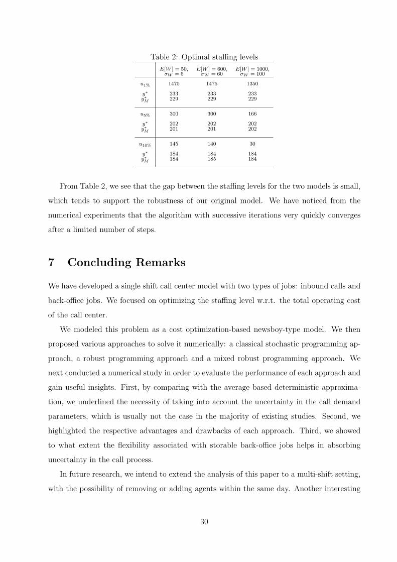
Table 2: Optimal staffing levels

E[W ] = 50, E[W ] = 600, E[W ] = 1000,σW = 5 σW = 60 σW = 100

u1% 1475 1475 1350

y∗ 233 233 233y∗M 229 229 229

u5% 300 300 166

y∗ 202 202 202y∗M 201 201 202

u10% 145 140 30

y∗ 184 184 184y∗M 184 185 184

From Table 2, we see that the gap between the staffing levels for the two models is small,

which tends to support the robustness of our original model. We have noticed from the

numerical experiments that the algorithm with successive iterations very quickly converges

after a limited number of steps.

7 Concluding Remarks

We have developed a single shift call center model with two types of jobs: inbound calls and

back-office jobs. We focused on optimizing the staffing level w.r.t. the total operating cost

of the call center.

We modeled this problem as a cost optimization-based newsboy-type model. We then

proposed various approaches to solve it numerically: a classical stochastic programming ap-

proach, a robust programming approach and a mixed robust programming approach. We

next conducted a numerical study in order to evaluate the performance of each approach and

gain useful insights. First, by comparing with the average based deterministic approxima-

tion, we underlined the necessity of taking into account the uncertainty in the call demand

parameters, which is usually not the case in the majority of existing studies. Second, we

highlighted the respective advantages and drawbacks of each approach. Third, we showed

to what extent the flexibility associated with storable back-office jobs helps in absorbing

uncertainty in the call process.

In future research, we intend to extend the analysis of this paper to a multi-shift setting,

with the possibility of removing or adding agents within the same day. Another interesting

30

extension would be to consider a global service level constraint for the whole day, instead of

having a period by period constraint.

Appendix

A Proof of Theorem 1

We assume that C(y) is a continuous function over y ∈ R+, Θ and W are continuous random

variables. It is clear that proving the convexity in the continuous case implies proving it for

the original discrete case. We denote by fΘ(.) and fW (.) (FΘ(.) and FW (.)) the probability

density functions ( the cumulative probability distribution functions) of the random variables

Θ and W , respectively. For a given outcome of Θ, denoted by θ, we use vi(θ) to denote the

required number of agents to handle the calls in period i. And Vi denotes the underlying

random number of agents required to handle calls in period i. The continuous version of the

total cost, given in Equation (6) becomes

C(y) = n c y + uα

n∑i=1

∫ ∞

θ∗i (y)

(vi(θ)− y)fΘ(θ) dθ + r

∫ ∞

Q(y)

(x−Q(y))fW (x) dx, (60)

where

Q(y) = E[n∑

i=1

(y − Vi)+] =

n∑i=1

∫ θ∗i (y)

0

(y − vi(θ))fΘ(θ) dθ, (61)

θ∗i (y) = min{θ : vi(θ) ≥ y}, i = 1, .., n. (62)

Proving the convexity of the C(·) function is equivalent to prove thatd2C(y)

dy2≥ 0 for

y ∈ R+. Applying Leibniz formula, we have

dQ(y)

dy=

n∑i=1

∫ θ∗i (y)

0

fΘ(θ) dθ =n∑

i=1

FΘ(θ∗i (y)). (63)

Combining now Equations (60) and (63), we obtain

31

dC(y)

dy= nc− uα

n∑i=1

∫ ∞

θ∗i (y)

fΘ(θ)dθ + r

∫ ∞

Q(y)

∂(x−Q(y)

)∂y

fW (x)dx (64)

= nc+ uα

(n∑

i=1

FΘ(θ∗i (y))− n

)− r

∫ ∞

Q(y)

n∑i=1

FΘ(θ∗i (y)) fW (x)dx (65)

= n(c− uα) +(uα − r

(1− FW (Q(y))

)) n∑i=1

FΘ(θ∗i (y)). (66)

We have

d2C(y)

dy2=

d

dy

((uα − r

(1− FW (Q(y))

))·

n∑i=1

FΘ(θ∗i (y))

). (67)

Since for i = 1, ..., n, FΘ(·) ≥ 0 and F ′Θ(·) ≥ 0, FW (·) ≥ 0 and F ′

W (·) ≥ 0 and by assumption

r < uα ( see Section 3), we have

uα − r(1− FW (Q(y))

)≥ 0, (68)

andd

dy

(uα − r

(1− FW (Q(y))

))= r

dFW (Q(y))

dy≥ 0. (69)

We thereafter conclude thatd2C(y)

dy2≥ 0, which finishes the proof of the theorem.

2

B Proof of Proposition 1

Recall that C(y, θ, w) is the cost associated with a given staffing level y, a “business” level

θ and a back-office workload w as defined in Equation (7). For given sample values θ and

w, we denote the optimal solution of problem (21)-(25) as y∗θ,w. Furthermore, for a given

staffing level y, and sample values θ and w, we denote the corresponding variables Mθ, w, i(y),

M−θ, w, i(y), M

+θ, w, i(y) and Nθ, w(y). We now prove that for δ ≥ 0, we have C(y∗θ+δ, w, θ, w) ≤

C(y∗θ+δ, w, θ + δ, w).

It is straight forward to see that the variables M−θ, w, i(y) and M+

θ, w, i(y) can not take

strictly positive values, simultaneously. In case of over-staffing (under-staffing) at period i,

32

we have M+θ, w, i(y) > 0 and M−

θ, w, i(y) = 0 ( M+θ, w, i(y) = 0 and M−

θ, w, i(y) > 0).

Furthermore, using the Erlang C formula, we have for each period i, vi(θ fi) ≤ vi((θ +

δ) fi). For the staffing level y∗θ+δ, w, we have Mθ, w, i(y∗θ+δ, w) ≥ Mθ+δ, w, i(y

∗θ+δ, w), which means

M+θ, w, i(y

∗θ+δ, w) ≥ M+

θ+δ, w, i(y∗θ+δ, w) and M−

θ, w, i(y∗θ+δ, w) ≤ M−

θ+δ, w, i(y∗θ+δ, w). Furthermore,

by constraint (24), we have Nθ, w(y∗θ+δ, w) ≤ Nθ+δ, w(y

∗θ+δ, w). As n, c, uα, r > 0, we easily get

C(y∗θ+δ, w, θ, w) ≤ C(y∗θ+δ, w, θ+δ, w). Since C∗(θ, w) = miny∈NC(y, θ, w), we have C∗(θ, w) ≤

C(y∗θ+δ, w, θ, w). Therefore C∗(θ, w) ≤ C∗(θ + δ, w), which gives (26).

Consider now sample values θ and w + δ, with δ > 0. For a given staffing level y,

by constraint (22), we have Mθ, w, i(y) = Mθ, (w+δ), i(y), and Nθ, w(y) ≤ Nθ, w+δ(y). This

leads to C(y∗θ, w+δ, θ, w) ≤ C(y∗θ, w+δ, θ, w + δ). Since C∗(θ, w) ≤ C(y∗θ, w+δ, θ, w), we obtain

C∗(θ, w) ≤ C∗(θ, w+δ), which gives (27). 2

C Mixed Robust Programming Formulation

Here we give a formulation mixing stochastic and robust programming (see the end of Section

4.2). With an uncertainty set for Θ defined as

U ′ = {θ : 0 ≤ θ ≤ θ + η σθ, with η ≥ 0} (70)

and with the random back-office workload process described as in Section 3.2, a mixed robust

programming formulation can be given as follows:

Min nc y + uα

n∑i=1

M−i + r

K∑k=1

pwkNk (71)

s.t. Mi = y − vi((θ + η σθ)fi), with i = 1, ..., n, (72)

Mi = M+i −M−

i , with i = 1, ..., n, (73)

Nk ≥ wk −n∑

i=1

M+i, l, with k = 1, ..., K, (74)

y,M+i ,M

−i , Nk ≥ 0, with i = 1, ..., n, k = 1, ..., K. (75)

In this problem, Mi represents the difference between the staffing level and the required agent

number in period i for the highest arrival rate in the considered uncertainty set, (θ+ η σθ)fi.

Nk is the over-time workload required in order to finish back-office jobs in scenario k.

33

D Additional Numerical Results

In Tables 3 and 4, we give additional support for the numerical analysis of Section 5.1.3.

34

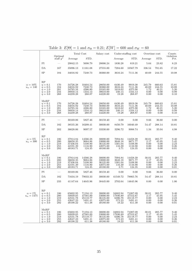
Table 3: E[Θ] = 1 and σΘ = 0.21; E[W ] = 600 and σW = 60

Total Cost Salary cost Under-staffing cost Overtime cost Constr.Optimal violationstaff y∗ Average STD. Average STD. Average STD. Pct.

PI — 29842.15 5698.79 28006.24 1830.28 819.21 5.64 23.82 8.23

DA 167 35096.13 11161.08 27555.00 7204.60 10567.79 336.54 781.65 17.22

SP 184 34016.92 7248.73 30360.00 3616.24 7111.36 40.69 244.55 10.08

RPα = 10% η = 0.1 170 34726.28 10404.54 28050.00 6430.49 9919.38 245.79 660.63 15.81uα = 140 η = 0.5 184 34016.92 7248.73 30360.00 3616.24 7111.36 40.69 244.55 10.08

η = 1.0 201 34785.34 4386.80 33165.00 1618.62 4375.90 1.72 40.21 5.20η = 2.0 234 38850.14 1334.13 38610.00 240.14 1334.13 0.00 0.00 0.99η = 3.0 268 44239.28 268.87 44220.00 19.28 268.87 0.00 0.00 0.10

MxRPη = 0.1 170 34726.28 10404.54 28050.00 6430.49 9919.38 245.79 660.63 15.81η = 0.5 184 34016.92 7248.73 30360.00 3616.24 7111.36 40.69 244.55 10.08η = 1.0 201 34785.34 4386.80 33165.00 1618.62 4375.90 1.72 40.21 5.20η = 2.0 234 38850.14 1334.13 38610.00 240.14 1334.13 0.00 0.00 0.99η = 3.0 268 44239.28 268.87 44220.00 19.28 268.87 0.00 0.00 0.10

PI — 30169.06 5827.46 30159.40 0.00 0.00 9.66 36.60 0.00

DA 182 38535.26 16209.41 30030.00 8450.79 16040.49 54.47 288.14 10.81

SP 202 36628.06 9097.57 33330.00 3296.72 9088.74 1.34 35.04 4.98

RPα = 5% η = 0.1 186 37814.84 14566.28 30690.00 7094.84 14458.39 30.01 205.77 9.40uα = 300 η = 0.5 200 36650.35 9684.86 33000.00 3648.18 9671.77 2.17 45.95 5.45

η = 1.0 219 37436.04 5108.90 36135.00 1301.04 5108.90 0.00 0.00 2.23η = 2.0 255 42191.39 1116.90 42075.00 116.39 1116.90 0.00 0.00 0.26η = 3.0 292 48183.71 124.35 48180.00 3.71 124.35 0.00 0.00 0.01

MxRPη = 0.1 186 37814.84 14566.28 30690.00 7094.84 14458.39 30.01 205.77 9.40η = 0.5 200 36650.35 9684.86 33000.00 3648.18 9671.77 2.17 45.95 5.45η = 1.0 219 37436.04 5108.90 36135.00 1301.04 5108.90 0.00 0.00 2.23η = 2.0 255 42191.39 1116.90 42075.00 116.39 1116.90 0.00 0.00 0.26η = 3.0 292 48183.71 124.35 48180.00 3.71 124.35 0.00 0.00 0.01

PI — 30169.06 5827.46 30159.40 0.00 0.00 9.66 36.60 0.00

DA 182 71634.19 79033.33 30030.00 41549.72 78865.76 54.47 288.14 10.81

SP 233 41147.64 14645.96 38445.00 2702.64 14645.96 0.00 0.00 1.06

RPα = 1% η = 0.1 186 65602.95 71194.13 30690.00 34882.94 71087.09 30.01 205.77 9.40

uα = 1475 η = 0.5 200 50939.05 47565.89 33000.00 17936.89 47552.87 2.17 45.95 5.45η = 1.0 219 42531.78 25118.77 36135.00 6396.78 25118.77 0.00 0.00 2.23η = 2.0 255 42647.23 5491.41 42075.00 572.23 5491.41 0.00 0.00 0.26η = 3.0 292 48198.22 611.38 48180.00 18.22 611.38 0.00 0.00 0.01

MxRPη = 0.1 186 65602.95 71194.13 30690.00 34882.94 71087.09 30.01 205.77 9.40η = 0.5 200 50939.05 47565.89 33000.00 17936.89 47552.87 2.17 45.95 5.45η = 1.0 219 42531.78 25118.77 36135.00 6396.78 25118.77 0.00 0.00 2.23η = 2.0 255 42647.23 5491.41 42075.00 572.23 5491.41 0.00 0.00 0.26η = 3.0 292 48198.22 611.38 48180.00 18.22 611.38 0.00 0.00 0.01

35

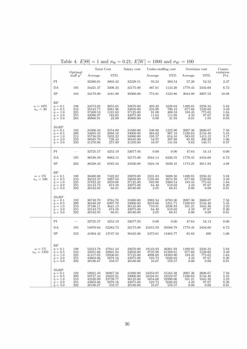
Table 4: E[Θ] = 1 and σΘ = 0.21; E[W ] = 1000 and σW = 100

Total Cost Salary cost Under-staffing cost Overtime cost Constr.Optimal violationstaff y∗ Average STD. Average STD. Average STD. Pct.

PI — 32380.01 3803.42 32229.51 93.24 269.54 57.26 52.52 2.47

DA 195 34421.47 3306.33 32175.00 467.01 1124.20 1779.45 2434.60 6.72

SP 184 34179.90 4181.90 30360.00 774.91 1523.86 3044.99 3007.52 10.08

RPα = 10% η = 0.1 198 34573.05 3055.65 32670.00 403.20 1028.04 1499.85 2256.24 5.94uα = 30 η = 0.5 210 35543.77 2081.96 34650.00 216.09 700.19 677.68 1529.68 3.49

η = 1.0 225 37409.53 1101.63 37125.00 91.08 408.53 193.45 775.65 1.64η = 2.0 255 42090.97 183.05 42075.00 11.64 111.69 4.33 97.67 0.26η = 3.0 284 46860.91 22.09 46860.00 0.90 21.93 0.01 1.05 0.03

MxRPη = 0.1 192 34306.34 3554.89 31680.00 538.98 1225.90 2087.36 2606.67 7.56η = 0.5 200 34695.45 2888.18 33000.00 364.82 967.18 1330.63 2134.48 5.45η = 1.0 212 35756.59 1932.22 34980.00 193.57 654.10 583.02 1415.12 3.17η = 2.0 233 38585.79 728.44 38445.00 54.97 297.88 85.82 490.39 1.06η = 3.0 250 41276.60 257.09 41250.00 16.97 141.93 9.63 146.71 0.37

PI — 32725.57 4252.19 32677.93 0.00 0.00 47.64 54.13 0.00

DA 195 36538.59 8082.15 32175.00 2584.14 6220.55 1779.45 2434.60 6.72

SP 202 36328.43 6585.24 33330.00 1824.18 5029.10 1174.25 2011.94 4.98

RPα = 5% η = 0.1 198 36400.88 7422.82 32670.00 2231.03 5688.50 1499.85 2256.24 5.94uα = 166 η = 0.5 210 36523.37 5067.04 34650.00 1195.69 3874.39 677.68 1529.68 3.49

η = 1.0 225 37822.42 2859.08 37125.00 503.98 2260.54 193.45 775.65 1.64η = 2.0 255 42143.73 674.59 42075.00 64.40 618.02 4.33 97.67 0.26η = 3.0 292 48182.05 68.81 48180.00 2.05 68.81 0.00 0.00 0.01

MxRPη = 0.1 192 36749.70 8764.76 31680.00 2982.34 6783.30 2087.36 2606.67 7.56η = 0.5 200 36349.29 6997.70 33000.00 2018.66 5351.71 1330.63 2134.48 5.45η = 1.0 219 37186.11 3641.13 36135.00 719.91 2826.93 331.21 1045.39 2.23η = 2.0 255 42143.73 674.59 42075.00 64.40 618.02 4.33 97.67 0.26η = 3.0 292 48182.05 68.81 48180.00 2.05 68.81 0.00 0.00 0.01

PI — 32725.57 4252.19 32677.93 0.00 0.00 47.64 54.13 0.00

DA 195 54970.04 52282.73 32175.00 21015.59 50588.78 1779.45 2434.60 6.72

SP 233 41004.42 13747.43 38445.00 2473.61 13404.77 85.82 490 1.06

RPα = 1% η = 0.1 198 52313.78 47841.24 32670.00 18143.93 46261.93 1499.85 2256.24 5.94

uα = 1350 η = 0.5 210 45051.66 32601.04 34650.00 9723.98 31508.61 677.68 1529.68 3.49η = 1.0 225 41417.05 18936.65 37125.00 4098.60 18383.90 193.45 775.65 1.64η = 2.0 255 42603.06 5078.16 42075.00 523.73 5026.03 4.33 97.67 0.26η = 3.0 292 48196.67 559.57 48180.00 16.67 559.57 0.00 0.00 0.01

MxRPη = 0.1 192 58021.33 56967.56 31680.00 24253.97 55165.38 2087.36 2606.67 7.56η = 0.5 200 50747.44 45022.91 33000.00 16416.81 43522.97 1330.63 2134.48 5.45η = 1.0 219 42320.89 23739.77 36135.00 5854.68 22990.06 331.21 1045.39 2.23η = 2.0 255 42603.06 5078.16 42075.00 523.73 5026.03 4.33 97.67 0.26η = 3.0 292 48196.67 559.57 48180.00 16.67 559.57 0.00 0.00 0.01

36

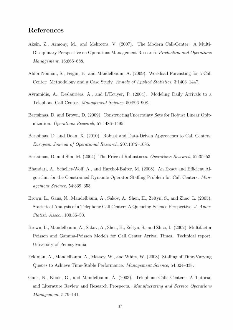
References

Aksin, Z., Armony, M., and Mehrotra, V. (2007). The Modern Call-Center: A Multi-

Disciplinary Perspective on Operations Management Research. Production and Operations

Management, 16:665–688.

Aldor-Noiman, S., Feigin, P., and Mandelbaum, A. (2009). Workload Forcasting for a Call

Center: Methodology and a Case Study. Annals of Applied Statistics, 3:1403–1447.

Avramidis, A., Deslauriers, A., and L’Ecuyer, P. (2004). Modeling Daily Arrivals to a

Telephone Call Center. Management Science, 50:896–908.

Bertsimas, D. and Brown, D. (2009). ConstructingUncertainty Sets for Robust Linear Opit-

mization. Operations Research, 57:1486–1495.

Bertsimas, D. and Doan, X. (2010). Robust and Data-Driven Approaches to Call Centers.

European Journal of Operational Research, 207:1072–1085.

Bertsimas, D. and Sim, M. (2004). The Price of Robustness. Operations Research, 52:35–53.

Bhandari, A., Scheller-Wolf, A., and Harchol-Balter, M. (2008). An Exact and Efficient Al-

gorithm for the Constrained Dynamic Operator Staffing Problem for Call Centers. Man-

agement Science, 54:339–353.

Brown, L., Gans, N., Mandelbaum, A., Sakov, A., Shen, H., Zeltyn, S., and Zhao, L. (2005).

Statistical Analysis of a Telephone Call Center: A Queueing-Science Perspective. J. Amer.

Statist. Assoc., 100:36–50.

Brown, L., Mandelbaum, A., Sakov, A., Shen, H., Zeltyn, S., and Zhao, L. (2002). Multifactor

Poisson and Gamma-Poisson Models for Call Center Arrival Times. Technical report,

University of Pennsylvania.

Feldman, A., Mandelbaum, A., Massey, W., and Whitt, W. (2008). Staffing of Time-Varying

Queues to Achieve Time-Stable Performance. Management Science, 54:324–338.

Gans, N., Koole, G., and Mandelbaum, A. (2003). Telephone Calls Centers: A Tutorial

and Literature Review and Research Prospects. Manufacturing and Service Operations

Management, 5:79–141.

37

Green, L. and Kolesar, P. (1991). The Pointwise Stationary Approximation for Queues with

Nonstationary Arrivals. Management Science, 37:84–97.

Green, L., Kolesar, P., and Soares, J. (2003). An Improved Heuristic for Staffing Telephone

Call Centers with Limited Operating Hours. Production and Operations Management,

12:46–61.

Green, L., Kolesar, P., and Whitt, W. (2007). Coping with Time-Varying Demand When

Setting Staffing Requirements for a Service System. Production and Operations Manage-

ment, 16:13–39.

Gross, D. and Harris, C. (1998). Fundamentals of Queueing Theory. Wiley Series in Proba-

bility and Mathematical Statistics. 3rd Edition.

Gurvich, I., Luedtke, J., and Tezcan, T. (2010). Staffing Call-Centers with Uncertain De-

mand Forecasts: A Chance-Constraints Approach. Management Science, 56:1093–1115.

Harrison, J. and Zeevi, A. (2005). A Method for Staffing Large Call Centers Based on

Stochastic Fluid Models. Manufacturing and Service Operations Management, 7:20–36.

Helber, S. and Henken, K. (2010). Profit-Oriented Shift Scheduling of Inbound Contact

Centers with Skills-Based Routing, Impatient Customers, and Retrials. OR Spectrum,

32:109–134.

Hur, D., Mabert, V., and Bretthauer, K. (2004). Real-Time Work Schedule Adjustment

Decisions: An Investigation and Evaluation. Production and Operations Management,

13:322–339.

Ingolfsson, A., Akhmetshina, A., Budge, S., Li, Y., and Wu, X. (2007). Survey and

Experimental Comparison of Service Level Approximation Methods for Nonstationary

M(t)/M/s(t) Queueing Systems. INFORMS Journal on Computing, 19:201–214.

Jongbloed, G. and Koole, G. (2001). Managing Uncertainty in Call Centers Using Poisson

Mixtures. Applied Stochastic Models in Business and Industry, 17:307–318.

Natarajan, K., Pachamanova, D., and Sim, M. (2009). Constructing Risk Measures from

Uncertainty Sets. Operations Research, 57(5):1129–1141.

38

Ogryczak, W. and Ruszczynski, A. (2002). Dual Stochastic Dominance and Related Mean-

Risk Models. SIAM Journal on Optimization, 13:60–78.

Robbins, T. (2007). Managing Service Capacity under Uncertainty. Ph.D. Dissertation,

Penn State University.

Robbins, T. and Harrison, T. (2010). A Stochastic Programming Model for Scheduling Call

Centers with Global Service Level Agreements. European Journal of Operational Research,

207(3):1608–1619.

Robbins, T., Medeiros, D., and Harrison, T. (2007). Partial Cross Training in Call Centers

with Uncertrain Arrivals and Global Service Level Agreements. In Proceedings of the 2007

Winter Simulation Conference.

Robbins, T., Medeiros, D., and Harrison, T. (2008). Optimal Cross Training in Call Centers

with Uncertain Arrivals and Global Service Level Agreements. Working paper. Pennsyl-

vania State University.

Rockafellar, T. and Uryasev, S. (2002). Conditional Value-at-Risk for General Loss Distri-

butions. Journal of Banking and Finance, 26:1443–1471.

Shen, H. and Huang, J. (2008). Interday Forecasting and Intraday Updating of Call Center

Arrivals. Manufacturing and Service Operations Management, 10:391–410.

Soyster, A. L. (1973). Convex Programming with Set-Inclusive Constraints and Applications

to Inexact Linear Programming. Operations Research, 21(5):1154–1157.

Steckley, S., Henderson, S., and Mehrotra, V. (2004). Service System Planning in the Pres-

ence of a Random Arrival Rate. Technical report, Cornell University, Ithaca, NY.

Stolletz, R. (2008). Approximation of the Non-Stationary M(t)/M(t)/c(t)-Queue using Sta-

tionary Queueing Models: The Stationary Backlog-Carryover Approach. European Journal

of Operational Research, 190(2):478–493.

Thenie, J., van Delft, C., and Vial, J. (2007). Automatic Formulation of Stochastic Programs

Via an Algebraic Modeling Language. Computational Management Science, 4:17–40.

39

Thompson, G. (1993). Accounting for The Multi-Period Impact of Service When Determin-

ing Employee Requirements for Labor Scheduling. Journal of Operations Management,

11(3):269–287.

van Delft, C. and Vial, J. (2004). A Practical Implementation of Stochastic Programming:

An Applications to the Evaluation of Option Contracts in Supply Chains. Automatica,

40:743–756.

Weinberg, J., Brown, L., and Stroud, J. (2007). Bayesian Forecasting of an Inhomogeneous

Poisson Process with Applications to Call Center Data. Journal of the American Statistical

Association, 102:1186–1199.

Whitt, W. (1999). Dynamic Staffng in a Telephone Call Center Aiming to Immediately

Answer All Calls. Operations Research Letters, 24:205–212.

Whitt, W. (2006). Staffing a Call Center with Uncertain Arrival Rate and Absenteeism.

Production and Operations Management, 15:88–102.

Yoo, J. (1996). Queueing Models for Staffing Service Operations. Ph.D. Dissertation, Uni-

versity of Maryland.

40