nurse absenteeism and staffing strategies for hospital ...isye.umn.edu/labs/scorlab/pdf/wg12.pdf ·...
TRANSCRIPT

Nurse Absenteeism and Staffing Strategies forHospital Inpatient Units
Wen-Ya Wang1, Diwakar Gupta21Marketing & Decision Sciences Department, San Jose State University2Industrial & Systems Engineering Department, University of Minnesota
Inpatient staffing costs are significantly affected by nurse absenteeism, which is typically high in US hospitals.
We use data from multiple inpatient units of two hospitals to study which factors, including unit culture,
short-term workload, and shift type, explain nurse absenteeism. The analysis highlights the importance
of paying attention to heterogeneous absentee rates among individual nurses. We then develop models to
investigate the impact of demand and absentee rate variability on the performance of staffing plans and
obtain some structural results. Utilizing these results, we propose and test three easy-to-use heuristics to
identify near optimal staffing strategies. Such strategies could be useful to hospitals that periodically re-
assign nurses with similar qualifications to inpatient units in order to balance workload and accommodate
changes in patient flow. Although motivated by staffing of hospital inpatient units, the approach developed
in this paper is also applicable to other team-based and labor-intensive service environments.
Key words : Absenteeism, Staffing, Hospital operations
1. Introduction
Inpatient units are often organized by nursing skills required to provide care. A typical classifi-
cation of inpatient units includes the following tiers: intensive care (ICU), step-down, and medi-
cal/surgical. Multiple units may exist within a tier, each with a somewhat different specialization.
For example, different ICUs may take care of a common pool of patients and in addition have a
few beds that are reserved for subpopulations such as cardiac and vascular, surgical, trauma, and
pediatric patients. Nurses whose skills are adequate for assignment to a particular type of unit may
be assigned to any one of the multiple units of that type, which is then called their home unit.
When nurses take care of a special subpopulation of patients within their home unit, they under-
take training that is specific to the needs of that patient group. Hospitals also provide periodic
learning opportunities to nurses to keep their skills up to date.
This paper focuses on the long-term staffing decision of assigning nurses with similar qualifica-
tions to their home units to rebalance workload and reduce understaffing costs due to unplanned
absences. The need to assign (or reassign) nurses to their home units may arise periodically due
to hospital reorganization, changes in demand patterns, and changes in practice norms (Sovie and
1

Wang and Gupta: Nurse Absenteeism and Staffing Strategies for Hospital Inpatient Units2
Jawad 2001, Bell et al. 2008, Sochalski et al. 1997). For example, if the hospital adds or loses
surgeons with privileges to perform certain types of surgeries, then the hospital may open, close,
or move beds to adapt to the resulting change in patient types and volumes. Re-organization of
inpatient units is also driven by technology and facility upgrades. Among the hospitals we have
interacted with, nurses’ home unit assignment is typically revisited annually.
Some hospitals create a pool of nurses, referred to as the float pool, who may be assigned to
different units depending on short-term variation in nursing needs. However, hospitals generally
do not dynamically assign non-float-pool nurses to different units to balance nursing needs in the
short term because of the potential negative impact on patient safety (especially when patient
requirements are different) and increased stress on nurses from working in unfamiliar physical envi-
ronments, using unfamiliar equipment, and having unfamiliar coworkers (Ferlise and Baggot 2009).
Some contract rules in fact prevent nurse managers from temporarily reassigning nurses to work
in different units (California Nurse Association and National Nurses Organizing Committee 2012).
Hence, an important long-term staffing decision is to find an allocation of non-float pool nurses
to different nursing units to minimize understaffing costs while accounting for nurses’ unplanned
absences.
Nurses’ absentee rates are high in U.S. hospitals. According to the Veterans Administration (VA)
Outcomes Database, the average unplanned absentee rate across all hospitals in the VA Health
Care System was 6.4% for a 24-week period between September 2011 and February 2012. [In the VA
data, unplanned absences include sick leaves and leaves without pay.] This statistic is significantly
higher than absentee rates among healthcare practitioner/technical occupations and all occupations
in the United States, which happen to be 3.7% and 3% respectively (Bureau of Labor Statistics
2011), underscoring the importance of considering absenteeism in nurse staffing models. We argue
in this paper that in addition to balancing demand and supply, careful assignment of nurses to
their home units can help lower staffing costs due to unplanned nurse absenteeism.
Hospitals face significant variation in demand for nursing services; see Section 2.1 for empirical
evidence from two hospitals. Nurse absenteeism exacerbates the difficulty of matching supply and
demand for nursing services in an economical manner. Nurse shortage jeopardizes quality of care
and patients’ safety, increases length of stay, and lowers nurses’ job satisfaction (e.g. Unruh 2008,
Aiken et al. 2002, Needleman et al. 2002, Cho et al. 2003, Lang et al. 2004, and Kane et al. 2007).
For these reasons, hospitals generally find replacements to fill in absent shifts as much as possible
even if this practice is costly. For example, in one of the hospitals discussed in this paper, the total

Wang and Gupta: Nurse Absenteeism and Staffing Strategies for Hospital Inpatient Units3
overtime cost was about 2.3 million per 2-week pay period. Therefore, implementable strategies
that could lower even a fraction of understaffing cost would be attractive to hospitals.
We formulate the problem of assigning a cohort of nurses to their home units as a discrete
stochastic optimization problem, which is a combinatorially hard problem. The practical usefulness
of our model depends on the characterization of a function that maps assignment of nurses to the
random number of nurses who show up in each unit. To characterize such mapping, we utilize
computerized records from multiple nursing units of two health systems and develop a statistical
model to explain nurse absenteeism. We conclude that nurse absence patterns can be explained by
heterogeneous absentee rates among nurses while controlling for shift effect.
Because variability in absenteeism and the extent to which some nurses may be similar to others
in terms of their pattern of absenteeism will vary from one hospital to another, we consider three
different functional forms of absenteeism within the stochastic integer program. These are: (1)
deterministic, (2) random aggregate, and (3) nurse-specific Bernoulli. The first model assumes that
the number of absences is a deterministic function of the number of nurses assigned to a unit. This
model will be appropriate when nurse absences are predictable and it is the variability in demand
that drives staffing decisions. In this paper, it serves largely as a benchmark and as a mean-value
approximation of the underlying stochastic optimization problem. It also serves to highlight the
importance of making sure that assignments match average supply to mean demand in each unit.
The second model groups nurses into subsets such that nurses within a subset are homogeneous,
but each subset has a different absentee rate distribution. The third model can be viewed as a
special case of the second model in which each subset is of size 1, i.e. each nurse is different and
the overall absentee rate distribution of a unit is the convolution of absentee rate distributions of
particular nurses assigned to that unit.
Using stochastic orders, we show that greater variability in demand and attendance patterns
increases a hospital’s costs, and that for a fixed overall absentee rate, each unit’s cost is mini-
mized by choosing a more heterogeneous cohort of nurses. This suggests that a desirable staffing
plan will maximize heterogeneity within a unit but create demand-adjusted uniform plans across
units. Whereas the effect of increased variability is consistent with intuition, the desirability of a
heterogeneous cohort of nurses is not. In order to explain this finding, we also show that greater
heterogeneity leads to smaller variance in attendance patterns of the cohort of nurses assigned to
a unit. This qualitative insight can be extrapolated to other settings in which work is performed
by teams of employees.

Wang and Gupta: Nurse Absenteeism and Staffing Strategies for Hospital Inpatient Units4
In addition to establishing the above qualitative staffing guidelines, we also establish that the
hospital’s objective function is supermodular. [A function f : Rk → R is supermodular if f(x ∨
y) + f(x∧ y)≥ f(x) + f(y) for all x,y ∈Rk, where x∨ y denotes the componentwise maximum
and x ∧ y denotes the component wise minimum of x and y (Topkis 1998). If a function f is
supermodular, then function −f is submodular.] Because greedy heuristics generally work well
when objective function is supermodular (Topkis 1998, Il’ev 2001, Asadpour et al. 2008, Calinescu
et al. 2011), we explore greedy and one other heuristic for solving the staffing-plan optimization
problem. The two heuristics are compared to each other and a straw assignment heuristic. Both
heuristics are shown to work well in numerical experiments. The heuristics ensure a heterogeneous
combination of nurses within each nursing unit. We report the results of simulation experiments
using historical data, which realize savings of about 3-4% of understaffing costs upon following our
recommended heuristics relative to the straw heuristic. These experiments suggest that hospitals
can reduce staffing costs by utilizing historical attendance data and relatively easy-to-use heuristic
approaches for nurse assignment.
This paper makes a contribution to both operations management (OM) and health services
research (HSR) literatures. Its contribution to the OM literature comes from establishing certain
stochastic order relations and from obtaining qualitative staffing guidelines as well as easy-to-
use heuristics for making nurse assignments under different functional forms of absenteeism. Its
contribution to the HSR literature comes from testing a variety of potential predictors of nurse
absenteeism in a statistical model and corroborating survey-based results reported in the HSR
literature. We elaborate on these points below.
The staffing problem studied in this paper is similar to the random yield problem studied in
the OM literature in the sense that the realized staffing level (equivalently, the yield of good
items produced) may be lower than the planned staffing level (production lot size) due to nurses’
show uncertainty (random yield). Random yield models characterize yield uncertainty in one of
following ways: (1) For any given lot size n, the yield Q(n) is a binomial process with a yield rate
p; e.g. Grosfeld-Nir et al. (2000). (2) The yield is a product of the lot size and a random yield
rate (i.e. Q(n) = n · ξ, where n is the lot size, and ξ is the random yield rate); e.g. Gerchak et al.
(1988), Bollapragada and Morton (1999), Araman and Popescu (2010). (3) The production process
is in control for a period of time followed by a period when it is out of control (i.e. yield Q has
a geometric distribution); e.g. Grosfeld-Nir et al. (2000). (4) Yield is the result of having random
capacity to produce good units (i.e. Q = min{n,C}, where random C captures the unreliability
of the equipment); e.g. Ciarallo et al. (1994). (5) The distribution of yield is known (i.e. p(q|n) is

Wang and Gupta: Nurse Absenteeism and Staffing Strategies for Hospital Inpatient Units5
the probability of q good units given a lot size n); e.g. Gurnani et al. (2000). In addition, Yano
and Lee (1995) and Grosfeld-Nir and Gerchak (2004) contain comprehensive reviews of random
yield models. These models assume independent and homogeneous yield rates with the result that
the problem of determining how to put together production lots (equivalent to the composition of
nurses in our setting) does not arise in such settings. Our effort may be viewed as a generalization
of random yield models to a situation in which yield rate is different for each item.
Green et al. (2013) formulate a model with endogenous yield rates for medium-term nurse staffing
problems that occur at the unit level. The authors use data from one emergency department (ED)
of a single hospital and observe that nurses’ anticipated workload (measured by the ratio of staffing
level in a shift and the long-term average census) is positively correlated with their absentee rate.
The results from our data analysis are significantly different from those reported in Green et al.
(2013). In particular, short-term workload does not have a consistent effect on absenteeism in our
data. The differences arise because of the fundamental differences in the types of data and problem
scenarios modeled, which we explain next. First, inpatient units and EDs face different demand
patterns and patients’ length of stay with patients staying significantly longer in inpatient units.
[According to surveys done in 2006 and 2010, average length of stay in emergency departments
(delay between entering emergency and being admitted or discharged) was 3.7 hours and 4.1 hours
respectively (Ken 2006, Anonymous 2010). In contrast, the average length of inpatient stay in
short-stay hospitals was 4.8 days according to 2007 data (Table 99, part 3 in National Center for
Health Statistics 2011).] Second, it may be argued that EDs present a particularly stressful work
environment for nurses and therefore ED nurses may react differently to workload variation than
nurses who work in inpatient units. Third, we use data from multiple units, which allows us to
examine whether the impact of workload and other covariates on absentee rate is unit-specific or
consistent across units, whereas Green et al. (2013) examine data from a single ED.
Much of the OM literature dealing with nurse staffing has focused on developing nurse schedules
to minimize costs while satisfying nurses’ work preferences; see Lim et al. (2011) for a recent
review. These works are not closely related to our paper. There are numerous papers that are
motivated by applications outside healthcare domain that take into account staff absenteeism; see
e.g. Hur et al. (2004), Whitt (2006) and Blumenfeld and Inman (2009). However, to the best of
our knowledge, they do not focus on identifying predictors of absenteeism or assigning personnel
with heterogeneous absentee rates to different work units.
Some papers in the HSR literature explain why nurses take unplanned time off; see Davey et al.
(2009) for a systematic review. This literature concludes that nurse absences may be associated

Wang and Gupta: Nurse Absenteeism and Staffing Strategies for Hospital Inpatient Units6
with nurses’ personal characteristics (e.g. Laschinger and Grau 2012), prior attendance records
(e.g. Roelen et al. 2011), organizational norms or leadership styles of nurse managers (e.g. Schreuder
et al. 2011), and chronic work overload and burn out (e.g. Rajbhandary and Basu 2010). Our
results are consistent with this literature and contribute to it by presenting quantitative evidence
that each nurse’s attendance history is a predictor of his or her future absences. Note that the
majority of previous studies cited above are based on nurses’ self reported surveys.
The remainder of this paper is organized as follows. Section 2 formulates the nurse assignment
problem and presents statistical analyses to support the proposed absenteeism models. Section 3
discusses the properties of an optimal staffing strategy that leads to the proposed staffing heuristics,
and provides numerical examples comparing performance of different staffing strategies. Section 4
concludes the paper.
2. Model Formulation and Analysis
Suppose there are u inpatient units that require nurses with a particular skill set, n nurses with this
skill set are available for a particular shift type (e.g. Day shift), and these nurses can be divided
into m types based on their absentee rates. In particular, nurses that belong to the same type have
the same probability or pattern of being absent in an arbitrary shift. At one end of the spectrum
when m = n, every nurse is different. At the other end, when m = 1 all nurses are identical. In
general, a nurse manager may choose 1 ≤m≤ n to classify nurses. The objective is to minimize
expected total cost and the staffing-plan optimization problem can formulated as follows.
minaπ(a) =
u∑
i=1
E(
co(Xi−Qi(a))+)
, subject to∑u
i=1 a(i)t ≤ nt, t∈ {1, · · · ,m} and a ∈A, (1)
where co(·) is a function that captures the cost of understaffing resulting from utilizing over-
time/float/agency nurses, or reduced service and cancellations, Xi is unit i’s demand for nursing
services for the chosen shift type, Qi(a) denotes the random number of nurses who show up for
work in unit i under assignment a and A=×ui=1([0, n1]× [0, n2] · · · × [0, nm]) is the set of all possi-
ble nurse assignments. The decision variables are the components of matrix a, where the (i, j)-th
element is 1 if nurse i is assigned to work in unit j, and 0 otherwise. The expectation is taken over
all possible realizations of Xi and Qi(a) and (x− q)+ = max{x− q,0}. This staffing problem is
non-trivial because there are nu possible nurse assignments, each of which could lead to a different
cost.
The model specification is not complete until we specify the functional form of Qi(a), which
drives nurse allocation decisions. For example, if nurses are homogeneous, it does not matter which
Wang and Gupta: Nurse Absenteeism and Staffing Strategies for Hospital Inpatient Units7
nurses are assigned to which units. In contrast, if nurses are heterogeneous, the particular cohort
of nurses assigned to a unit does matter. Therefore, we first study staffing and absence data from
two health systems to ascertain the functional form of Qi(a) in Section 2.1. This allows us to
choose factors that potentially constitute Qi(a) including unit index, nurses who are assigned,
shift time, month, holiday, weather, and workload. The choice of such factors are also based on
interactions with nurse managers and findings in previous studies. Then, we test which factors
should be included in the stochastic optimization model by analyzing a statistical model.
2.1. Evidence from Data
We studied de-identified census and absentee records from two hospitals located in a large
metropolitan area. Census and absentee data from Hospital 1 were for the period January 3, 2009
through December 4, 2009, whereas Hospital 2’s data were for the period September 1, 2008 through
August 31, 2009. Basic information about these hospitals from fiscal year 2009 is summarized in
Table 6 in Appendix A. The differences between the maximum and the minimum patient census
in 2009 were 52.7% and 49.5% of the average census for Hospitals 1 and 2, respectively, indicating
that the overall variability in nursing demand was high. Patients’ average lengths of stay were 4.0
and 4.9 days and registered nurse (RN) salary accounted for 17.9% and 15.5% of total operating
expenses of the two hospitals.
Hospital 1 had five shift types. There were three 8-hour shifts designated Day, Evening, and Night
shifts, which operated from 7 AM to 3 PM, 3 PM to 11 PM, and 11 PM to 7 AM, respectively. There
were also two 12-hour shifts, which were designated Day-12 and Night-12 shifts. These operated
from 7 AM to 7 PM, and 7 PM to 7 AM, respectively. Hospital 2 had only three shift types,
namely the 8-hour Day, Evening, and Night shifts. Hospital 1’s data pertained to three step-down
(telemetry) units labeled T1, T2, and T3 with 22, 22, and 24 beds, and Hospital 2’s data pertained
to two medical/surgical units labeled M1 and M2 with 32 and 31 beds. The common data elements
were hourly census, admissions, discharges, and transfers, planned and realized staffing levels, and
the count of absentees for each shift. Hospital 1’s data also contained individual nurses’ attendance
history.
Both hospitals used target nurse-to-patient ratios to describe the desirable workload for their
inpatient units. The target ratios were determined by panels of experts (mostly experienced nurse
managers) in each hospital. Hospital 1’s target nurse-to-patient ratios for telemetry units were 1:3
for Day and Evening shifts during week days and 1:4 for Night and weekend shifts. Hospital 2’s
target nurse-to-patient ratios for medical/surgical units were 1:4 for Day and Evening shifts and
1:5 for Night shifts. Hospital 1’s planned staffing levels were based on the mode of the midnight

Wang and Gupta: Nurse Absenteeism and Staffing Strategies for Hospital Inpatient Units8
census in the previous planning period. Nurse managers would further tweak the staffing levels up
or down to account for holidays and to meet nurses’ planned-time-off requests and shift preferences.
Hospital 2’s medical/surgical units had fixed staffing levels based on the long-run average patient
census by day-of-week and shift. In both cases, staff planning was done in 4-week increments
and planned staffing levels were posted 2-weeks in advance of the first day of each 4-week plan.
Consistent with the fact that average lengths of stay in these hospitals were between 4 and 5 days,
staffing levels were not based on a projection of short-term demand forecast. When the number
of patients assigned to some nurses exceeded the target nurse-to-patient ratios, nurse managers
attempted to increase staffing by utilizing extra-time or overtime shifts, or calling in agency nurses.
Similarly, when census was less than anticipated, nurses were assigned to indirect patient care
tasks or education activities, or else asked to take voluntary time off. These efforts were not always
successful and realized nurse-to-patient ratios often differed from the target ratios. For example,
Hospital 1’s unit T3 on average staffed lower than the target ratios, whereas Hospital 2’s unit M2
on average staffed higher than the target ratios during weekends; see Figure 1 where the solid dots
were plotted at (mean, standard deviation) pairs of number of patients per nurse corresponding
to the horizontal (resp. vertical) axises by shift type and the 95% confidence intervals of the mean
were drawn along the horizontal lines.
In addition to the two hospitals whose data are analyzed in this paper, the authors have interacted
with nurse managers at numerous other urban hospitals. Staffing practices do vary from one hospital
to another. However, the range of practices prevalent at these two hospitals are representative of
many other hospitals. That is, models based on such practices should be useful for other hospitals
as well.
Figure 1 Average Number of Patients Per Nurse by Shift Type
2.5 3.0 3.5 4.0 4.5 5.0
0.4
0.6
0.8
1.0
1.2
1.4
Avg Number of Patients Per Nurse
SD
of N
umbe
r of
Pat
ient
s P
er N
urse
T1 (D/E)
T2 (D/E)
T3 (D/E)
T1 (N)
T2 (N)
T3 (N)
M1 (D/E)M2 (D/E)
M1 (N)
M2 (N)
TR 1 TR 2 TR 3
Note: SD = Standard Deviation. Avg = Average. D = Day. E = Evening. N = Night. TR 1 = Target ratio for T1,T2, and T3 in D and E shifts during weekdays. TR 2 = Target ratio for T1, T2, and T3 in N shifts or weekends;TR 2 is also the target ratio for M1 and M2 in D and E Shifts. TR 3 = Target ratio for M1 and M2 in N shifts. Anumerical summary of these statistics is included in Table 7 of Appendix A.

Wang and Gupta: Nurse Absenteeism and Staffing Strategies for Hospital Inpatient Units9
The two hospitals’ data were analyzed independently because (1) the data pertained to different
time periods, (2) the target nurse-to-patient ratios were different for the two types of inpatient units,
and (3) the two hospitals used different staffing strategies. Based on nurse managers’ suggestion
and our initial analysis of data, which we describe in the next three paragraphs, we considered the
following potential predictor of nurse absenteeism: (1) individual nurses’ attendance history, (2)
unit index (which potentially captures factors that were unit specific, e.g. unit culture), (3) day of
week, (4) shift time, (5) month of year (season), (6) holiday, and (7) extreme weather. In addition,
we also considered workload because workload has been found to be correlated with absenteeism
in previous studies (e.g. Green et al. 2013).
Table 1 Summary Statistics for Individual Nurses’ Absentee Rates in Hospital 1’s Telemetry Units
T1 T2 T3Number of Nurses 50 45 58Mean 12.6% 12.5% 8.4%Median 7.9% 9.5% 6.8%Standard Deviation 12.9% 14.9% 6.1%Minimum 0% 0% 0%Maximum 63% 32% 27%25th Percentile 4.6% 5.3% 4.7%75th Percentile 16.5% 14.9% 11.1%Coefficient of Variation 1.02 1.2 0.7
Table 1 summarizes individual nurses’ absentee rate statistics for Hospital 1’s three telemetry
units. With a coefficient of variation of 1.02, 1.2, and 0.70 in units T1, T2, and T3, it is reasonable
to conclude that the absentee rates among nurses are highly variable and nurses are heterogeneous.
The high variability among individual nurses’ absentee rates can also be seen in Figure 2.
We calculated each Hospital-1 nurse’s quarterly absentee rate and found that there was not a
statistically significant difference in nurses’ absentee rates across different quarters. This suggests
that although absentee rates were highly variable among Hospital 1’s nurses, each individual nurses’
absentee rate was relatively stable across time. This observation supports our choice of nurses’
attendance history as a potential predictor of future absences.
The absentee rate among Hospital 1’s three telemetry units varied from 3.4% (T1, Sunday, Day
Shift) to 18.3% (T1, Saturday, Night Shift) depending on unit, shift time, and day of week. Simi-
larly, the absentee rate for Hospital 2’s medical/surgical units varied from 2.99% (M1, Wednesday,
Evening Shift) to 12.98% (M2, Tuesday, Evening Shift) depending on unit, shift time, and day of
week. The 95% confidence intervals for absentee rates did not overlap across all units and shift

Wang and Gupta: Nurse Absenteeism and Staffing Strategies for Hospital Inpatient Units10
Figure 2 Absentee Rate Distribution (Boxplots) for Nurses in Hospital 1’s Telemetry Units
T1
T2
T3
Unit
0% 20% 40% 60%
Absentee Rate
Figure 3 Absentee Rate by Unit
0.06 0.07 0.08 0.09 0.10 0.11 0.12
0.09
0.11
0.13
Hospital 1
Avg Absentee Rate
SD
of A
bsen
tee
Rat
e T1
T2
T3
0.05 0.06 0.07 0.08 0.09 0.10
0.09
0.11
0.13
Hospital 2
Avg Absentee Rate
SD
of A
bsen
tee
Rat
e
M1
M2
Note: SD = Standard Deviation. Avg = Average. A numerical summary of these statistics is included in Table 8 ofAppendix A.
Figure 4 Absentee Rate by Shift Type
0.05 0.10 0.15 0.20 0.25
0.0
0.2
0.4
Hospital 1
Avg Absentee Rate
SD
of A
bsen
tee
Rat
e
D EN
D12
N12
0.05 0.06 0.07 0.08 0.09 0.10
0.0
0.2
0.4
Hospital 2
Avg Absentee Rate
SD
of A
bsen
tee
Rat
e
D E N
Note: SD = Standard Deviation. Avg = Average. A numerical summary of these statistics is included in Table 8 ofAppendix A.
types (Figures 3 and 4) but overlapped across all days of week (see Table 8 in Appendix A). These
statistics suggest that absentee rates were significantly different by unit and shift, but not by the
day of week. We also compared absentee rates for regular days and holidays, and fair-weather
days and storm days. At 5% significance level, holidays had a lower average absentee rate than

Wang and Gupta: Nurse Absenteeism and Staffing Strategies for Hospital Inpatient Units11
non holidays for Hospital 2 and storm days had a higher average absentee rate for Hospital 1. We
kept month as a potential predictors as there may be seasonality in absentee rates. A numerical
summary of absentee rates is included in Table 8 in Appendix A.
2.2. The Statistical Model
The observations in Section 2.1 suggest that absentee rates may vary by nurse, shift type, holiday,
weather, month of year, and workload. Although some of these factors will not be included in the
stochastic optimization model because either they are not actionable for long-term nurse assignment
decisions or their use is prevented by contract rules, we will include them in the statistical model
to obtain a more complete analysis. Note that only Hospital 1’s data contained individual nurses’
history of schedules. Hospital 2’s individual nurse records were not available.
To separate individual nurse effect from group-level effects, we fitted Hospital 1 data to the
following generalized linear mixed model (Equation (2)). The model assumes that each nurse j
has his or her own personal traits that contribute to absenteeism (a random-intercept model). In
addition, because the vast majority of the nurses (with only a few exceptions) work only in one
nursing unit during the time period covered by our dataset, the nurses are considered nested within
the inpatient units and we also treated unit effect as random. Note that the potential interaction
between unit and nurse assignment could not be evaluated with this data because very few nurses
were scheduled to work in more than one unit during the period. Our generalized linear mixed
model is the following.
log( pijt1− pijt
)
=Xijtβ+Li +Bij , (2)
where pijt is the absence probability for unit i’s nurse j when his or her t-th scheduled shift has
characteristics Xijt, β represents the coefficients for factors described in Xijt, Li is the random
effect explained by unit i, and Bij represents the nurse-j-specific intercept – i.e. nurse j’s impact
on his or her absenteeism that is not captured by Xijt and the unit effect. Note that Xijt is a
vector that captures information concerning the shift type (i.e. D, E, N, D12, or N12), standardized
workload (relative to the unit’s target workload, which we explain in next paragraphs), month
(i.e. January, · · · , December), holiday (i.e. non-holiday or holiday), weather (i.e. normal or extreme),
and the interaction between shift type and workload. We include the interaction between shift type
and workload because the target nurse to patient ratios for different shifts are not the same and
thus the impact of workload for different shifts may not be the same.

Wang and Gupta: Nurse Absenteeism and Staffing Strategies for Hospital Inpatient Units12
We measured unit i’s and shift t’s anticipated workload in three different ways: (1) w(1)it =
nit/E[Cit], (2) w(2)it =
∑m
i=1(ct−m/m)(1/nit), and (3) w(3)it =
∑m
i=1(ci(t−m)/m), where nit is the
planned staffing level, cit is unit i’s start-of-shift census for shift t, and E[Cit] is the long-run
expected census for unit i. Put differently, w(1)it equals the anticipated nurse-to-patient ratio; w
(2)it
equals the m-period moving average of estimated number of patients per nurse; and w(3)it equals the
m-period moving average of census. The choice of w(1)it is appropriate for units with stable nursing
demand, w(2)it for units in which both census and staffing levels vary from shift to shift, and w
(3)it
for units that have constant staffing levels (such as in Hospital 2).
In Equation (2), we used standardized workload w(k)it , which was calculated as follows: w(k)
it =(w
(k)it
−w(k)it
]
w(k)it
)
× 100%, where w(k)it is the workload at the target nurse-to-patient ratio for the shift
type to which shift t belongs for k = 1,2, and the average census for the shift type for k = 3. If
shift t’s anticipated workload equals its target nurse-to-patient ratio, then w(i)it =0. This allows us
to obtain a more intuitive interpretation of the coefficients that are related to shift and workload:
the shift coefficients can be explained as the shift effect at the target workload (when w(k)it = 0),
and the coefficients for w(k)it are the impact of a 1% increase or decrease in workload on absentee
rates.
2.3. Statistical Analysis Results
The model, regardless of workload variants, leads to a conclusion that individual nurses’ random
effect is much stronger than unit random effect. For the sake of brevity, complete details are
presented in Appendix B.1 and here we highlight our key findings. The standard deviation of Bij
is 3 to 7 times higher than the standard deviation of Li. In particular, the standard deviation of
Bij and Li are (0.75, 0.24), (0.75, 0.20), and (0.75, 0.11) for the three workload model variants,
respectively. This result supports the inference that unit effect is less important than individual
nurse effect, and hospitals may achieve greater efficiencies by periodically re-allocating some nurses
to different units.
Our goal is to identify actionable factors that can be utilized in the nurse assignment decisions.
For this reason, we check whether the fixed effects considered in Model (2) are consistent across
units by fitting the model to each unit separately. We drop the random unit effect Li in (2) and fit
the model to each unit one by one. The models of three workload variants lead to same conclusions.
Therefore, we only report the case with w(1)it in Table 2 for the sake of brevity. [Results for models
with w(2)it and w
(3)it when m= 6 are available in Tables 10 and 11 in Appendix B.2.] Note that for
workload models 2 and 3, we varied m (the moving average parameter) between 4 and 10 and the
conclusion from the statistical analysis remains the same.

Wang and Gupta: Nurse Absenteeism and Staffing Strategies for Hospital Inpatient Units13
Table 2 Result of the Statistical Model When Workload is Evaluated by w(1)it
Unit T1 T2 T3Rndom Effect: Standard Deviation Standard Deviation Standard DeviationNurse (Intercept) 0.873 0.621 0.638Fixed Effects: Est. S.E. P (> |z|) Est. S.E. P (> |z|) Est. S.E. P (> |z|)(Intercept) -2.578 0.261 <0.001∗ -2.448 0.216 <0.001∗ -3.144 0.267 <0.001∗
ShiftE 0.068 0.241 0.779 0.398 0.173 0.022∗ 0.521 0.255 0.041∗
ShiftN 0.893 0.287 0.002∗ 0.401 0.206 0.052 0.468 0.287 0.103ShiftD12 0.376 0.601 0.531 0.547 0.280 0.051 -1.666 0.558 0.003∗
ShiftN12 1.489 0.578 0.010∗ 0.321 0.271 0.236 -0.011 0.400 0.977
w(1)it 0.007 0.005 0.158 0.007 0.005 0.198 0.011 0.005 0.028
MonthFeb -0.002 0.234 0.995 -0.112 0.227 0.620 -0.001 0.228 0.995MonthMar -0.388 0.243 0.110 -0.142 0.228 0.534 -0.215 0.236 0.362MonthApr -0.056 0.228 0.807 -0.501 0.246 0.042∗ -0.115 0.230 0.618MonthMay -0.228 0.238 0.339 -0.239 0.241 0.322 -0.345 0.255 0.176MonthJun -0.192 0.238 0.419 -0.235 0.243 0.334 -0.257 0.238 0.279MonthJul -0.567 0.257 0.028∗ -0.022 0.240 0.926 0.232 0.225 0.302MonthAug -0.451 0.249 0.071 0.032 0.232 0.889 -0.066 0.227 0.770MonthSep -0.426 0.247 0.085 -0.568 0.267 0.033∗ -0.189 0.239 0.429MonthOct 0.156 0.224 0.485 0.271 0.215 0.206 0.405 0.208 0.052MonthNov -0.328 0.241 0.173 -0.076 0.232 0.744 -0.130 0.229 0.569MonthDec -1.191 0.570 0.037∗ -0.081 0.440 0.854 -0.991 0.620 0.110Holiday -0.126 0.361 0.726 -0.107 0.326 0.744 0.581 0.300 0.053Weather 0.704 0.325 0.030∗ 0.346 0.376 0.357 -0.372 0.449 0.407
ShiftE:w(1)it <0.001 0.007 0.965 0.001 0.007 0.883 -0.002 0.006 0.674
ShiftN:w(1)it -0.016 0.006 0.015∗ 0.002 0.007 0.775 -0.005 0.006 0.369
ShiftD12:w(1)it 0.070 0.033 0.033∗ 0.063 0.014 <0.001∗ 0.046 0.011 <0.001∗
ShiftN12:w(1)it 0.006 0.015 0.667 0.011 0.009 0.181 0.009 0.008 0.245
Standard Deviation: Standard deviation of the random intercepts.Est.: Estimate, S.E.: Standard Error of the Estimate, P (> |z|): p-value of Wald statistics.*: Significant at 0.05 level.
From Table 2, we observe that nurses’ random effect was strong (see the standard deviations of
the random intercepts). For example, when in unit T1 a D12 shift’s workload was 10% higher than
its average workload (i.e. w(1)it =−10% because a lower w
(1)it indicates a higher workload based on
the definition of w(1)it ), the log odds of absentee rate would decrease by 10× (0.007+ 0.07) = 0.77,
which was smaller than the standard deviation among nurses’ random intercepts (0.873). The
coefficients for month effects were also much smaller than the standard deviation of the random
intercepts for nurses. This suggests that nurses’ random effect on absenteeism was much stronger
than workload and month effects. The strong nurse random effects can also be observed in unit T2
and T3.
Among the fixed effects, we found that extreme weather was significant for unit T1, but not
T2 and T3. Holiday effect was not significant. Month effect was inconsistent across units — a

Wang and Gupta: Nurse Absenteeism and Staffing Strategies for Hospital Inpatient Units14
particular the month that has a higher or lower absentee rate for one unit does not have the same
effect for a different unit. In addition, even for the same unit, month effect is not consistent when
we use different workload measures in the model. It is possible that some units in some month of
the year have significantly higher or lower absentee rate. For example, it can happen that several
nurses in some month take unplanned sick days. however, without consistent pattern, such effect
cannot be the basis for long-term staffing decisions. Data show that monthly variations in absentee
rates require a short-term mitigation strategy because of the lack of a consistent pattern.
The impact of workload on absentee rates was not consistent across shifts and units for the
three variants of model (2) mentioned above, and the impact (if statistically significant) was small.
Furthermore, different w(k)it led to different conclusions for the same nursing unit. Take unit T1
in Table (2) as an example. The anticipated workload was negatively correlated with D12 shifts,
but positively correlated with Night shifts. Workload, when evaluated by w(2)it was significant for
N12 shift for T1, but not significant in T2 and T3 (Table 10 of Appendix B.2). Workload, when
evaluated by w(3)it was not significant for T2 (see Table 11 of Appendix B.2). Finally, if we take
into account the magnitude of random nurse effect, we see that the standard deviation of the
random intercept is much higher than the fixed effects due to workload. For these reasons, we
model heterogeneous nurses and do not incorporate workload in the long-term nurse assignment
problem.
When we look at shift effect at the target workload (i.e. w(1)it = 0), shift effects were not consistent
across units. T1’s Night and N12 shifts had a significantly higher absentee rates than Day, Evening,
and D12 shifts; T2’s Evening shifts had a higher absentee rates than Day shifts; T3’s Evening shifts
had a higher absentee rate and D12 shifts had a lower absentee rate than the other shifts. This
inconsistency may come from unit specific reasons that were not included in model. When we refer
back to the unit-pooled model (Table 9 in Appendix B.1) in which we evaluated shift effect for
all three units together while allowing random unit effects, we find that although some shifts type
might have higher or lower absentee rates, shift effects were weaker than the variability of nurse
random effects.
The above analysis shows that nurses have heterogeneous absentee rates and shift effect may
exist. We analyze the nurse assignment problem in (1) for each shift type. This approach is taken
because nurses’ shift work patterns are governed by their individual contracts and most nurses have
a primary work shift. We assume that when we re-assign nurses to different units, those nurses
will still be scheduled to work for the same shift time dictated by the contract rule. Although this
leaves open the possibility that shift effect may be be confounded with individual nurses’ absentee

Wang and Gupta: Nurse Absenteeism and Staffing Strategies for Hospital Inpatient Units15
pattern, our data does not allow us to tease out shift and nurse effects separately and the actionable
factor considered in Section 3 is the nurse-specific absentee rate.
3. Staffing Strategies
As mentioned in the Introduction section we consider three functional forms of Qi(a): (1) determin-
istic, (2) random aggregate, and (3) nurse-specific Bernoulli. These models are denoted by letters
d, r and b, respectively and notation needed for further analysis is summarized in Table 3. Note
that some of this notation was introduced earlier as part of model formulation. Although we have
identified that Qi(a) is driven by heterogeneous nurses who are assigned to the unit in Section 2,
we evaluate these three functional forms of Qi(a) in the staffing problem for the following reasons.
The deterministic functional form of Qi(a) is used to obtain a benchmark performance when a
nurse manager has perfect information about which nurses are going to be absent. The random
aggregate functional form of Qi(a) is used to evaluate the impact of variability in nurses’ absentee
rates. Finally, the nurse-specific Bernoulli model is used to capture the feature of heterogeneous
absentee rates to evaluate its impact on staffing. These three functional forms help us identify
characteristics of optimal staffing assignments.
Table 3 Notation
Indicesj = nurse index, j = 1, · · · , nt = nurse type index, t=1, · · · ,m; m≤ ni = unit index, i=1, · · · , uParametersp = (p1, · · · , pm), absent probabilities by nurse typen = (n1, · · · , nm), number of nurses by typeX = (X1, · · · ,Xu), (random) nursing needs vectorco(·) = an increasing convex shortage cost functionDecision Variables
a(i) = (a(i)1 , · · · , a
(i)m ), number of nurses assigned to unit i by type
a = (a(1), · · · ,a(u)), staffing planA = set of all possible assignments, A=×u
i=1([0, n1]× [0, n2] · · · × [0, nm])Calculated Quantitiesφi(a) = the number of absent nurses in unit i given assignment a
φ[k]i (a) = φi(a) under absentee model k, k ∈ {d, r, b}
Qi(a) =∑m
t=1 a(i)t −φi(a) = number of nurses who show up in unit i
πi(a) = total expected shortage cost for Unit i when staffing plan a is usedπ(a) = total expected shortage cost when staffing plan a is used =
∑u
i=1 πi(a)
The first model assumes that there is a deterministic mapping from a(i) to the number of
absentees, i.e. φi(a) = φ[d]i (a) ∈ [0,
∑m
t=1 a(i)t ]. The deterministic model does not represent reality

Wang and Gupta: Nurse Absenteeism and Staffing Strategies for Hospital Inpatient Units16
but serves as a benchmark mean value approximation of the underlying stochastic optimization
problem (Birge and Louveaux 2011). In the random aggregate model, nurse absence is viewed as
a group characteristic such that there is a type-specific random absence uncertainty ξt ∈ [0,1] for
each type-t nurse that is independent of a(i)t , and φ[r]i (a,ξ) =
∑m
t=1 a(i)t ξt. Note that this is similar
to the multiplicative random yield model studied extensively in the OM literature (see e.g. Yano
and Lee 1995). The third model is the closest to the functional form identified from the analysis of
Hospital 1 data. It considers each nurse as an independent decision maker with no-show probability
pt. In this case m = n and nt = 1 because each nurse is a type. The number of nurses who are
absent equals φi(a) = φ[b]i (a) =
∑n
t=1 a(i)t B(pt), where B(pt) is a Bernoulli random variable with
parameter pt, and each a(i)t is either 0 or 1.
In what follows, we index nurse types such that p1 ≥ p2 · · · ≥ pm and evaluate the effect of
demand variability and absentee rate variability on the performance of an assignment. For this
purpose, we use certain definitions and established results from the theory of stochastic orders
and majorization. These definitions and results are presented next. Further details can be found in
Shaked and Shanthikumar (2007), Marshall et al. (2011), and Liyanage and Shanthikumar (1992).
Definition 1. Given nursing requirement vectors X and X ′, X is said to be smaller than X ′
in the increasing convex order (X ≤icx X′) in a component-wise manner if E[g(Xi)] ≤ E[g(X ′
i)]
for every increasing convex function g for which the expectations exist and every i = 1, · · · , u.
Intuitively, if X ≤icx X ′, then X is both smaller and less variable than X ′ in some stochastic
sense.
Definition 2. Given vectors p and p′, where the components of these vectors are indexed such
that p1 ≥ p2 · · · ≥ pm, p′
1 ≥ p′2 · · · ≥ p′m, and∑m
t=1 pt =∑m
t=1 p′
t, we say that vector p is majorized by
p′, written p ≤M p′ if∑ℓ
t=1 pt ≤∑ℓ
t=1 p′
t for every ℓ ≤m. When the requirement of the equality∑m
t=1 pt =∑m
t=1 p′
t is dropped, we way that p′ weakly sub-majorizes p and is denoted p≤WM p′.
Majorization compares the dissimilarity of the components of a vector. Intuitively, if p≤M p′, then
components of p′ are more heterogeneous than p.
Definition 3. Let {Z(θ), θ ∈Θ} be a family of random variables with survival functions Fθ(z) =
P (Z(θ)> z), θ ∈Θ. The family {Z(θ), θ ∈Θ} is said to be stochastically increasing and linear in
the sense of the usual stochastic order, denoted SIL(st), if E[g(Z(θ))] is increasing linearly in θ for
all increasing functions g.
Theorem 1. (Shaked and Shanthikumar 2007, Theorem 8.C.1.) The family {Z(θ), θ ∈Θ} sat-
isfies {Z(θ), θ ∈Θ} ∈ SIL(st) if, and only if Fθ(z) is linear in θ for each fixed z.

Wang and Gupta: Nurse Absenteeism and Staffing Strategies for Hospital Inpatient Units17
Corollary 1. B(p) is SIL(st).
Proof of Corollary 1: Let b be a realization of a Bernoulli random variable B(p), where p is the
absentee rate. When b= 0, Fp(0) = 1. When b= 1, Fp(1) = p, which is increasing and linear in p.
Therefore, by Theorem 1, B(p) is SIL(st). �
Definition 4. A real-value function g defined on a set Θ⊂Rn is said to be Schur convex on Θ
if θ≤M θ′ on Θ⇒ g(θ)≤ g(θ′).
In other words, functions that preserve the ordering implied majorization are said to be Schur
convex.
Definition 5. A real valued random variable Z(θ) parameterized by θ ∈ Θ is stochastically
Schur convex in the sense of the usual stochastic [increasing convex] ordering if for any θ, θ′ ∈
Θ, θ ≤M θ′ implies Z(θ) ≤st [≤icx]Z(θ′). We denote this {Z(θ), θ ∈ Θ} ∈ S − SchurCX(st)[S −
SchurCX(icv)]. If in addition Z(θ) is stochastically increasing in θ, then Z(θ) is stochasti-
cally increasing and Schur convex. We denote this {Z(θ), θ ∈ Θ} ∈ SI − SchurCX(st)[SI −
SchurCX(icx)].
Theorem 2. (Liyanage and Shanthikumar 1992, Theorem 2.12.) Suppose {Zi(θ), θ ∈ Θ} ∈
SIL(st). Then for any increasing symmetric submodular [supermodular] function h and Z(θ) =
h(Z1(θ1), · · · ,Zm(θm)) one has {Z(θ), θ ∈Θm} ∈ SI−SchurCX(icv)[SI−SchurCV (icx)]. That is
for any θ, θ′ ∈Θm, increasing and symmetric sub modular [supermodular] function h and increasing
and concave [convex] function g,
θ≤WM θ′ ⇒Eg ◦h(Z1(θ1), · · · ,Zm(θm))≤Eg ◦h(Z1(θ′
1), · · · ,Zm(θ′
m)).
Now we are ready to analyze the properties of optimal nurse assignments. In what follows, we use
the asterisk notation to denote optimal quantities. In particular, a∗
α denotes an optimal assignment
of nurses when the problem is characterized by parameter α. For example, suppose X and X ′
denote two different nurse requirement vectors. Then, a∗
X and a∗
X′ are used to denote optimal
staffing plans with nurse requirements X and X ′, respectively. With these notation in hand, we
carry out stochastic comparisons to obtain the following results.
Proposition 1. If X ≤icx X′ in a component-wise sense, then π(a∗
X)≤ π(a∗
X′).
Proof for Proposition 1: Note that Xi ≤icx X′
i for each i = 1, · · · , u. Therefore, E[co(Xi −
Qi(a))+]≤E[co(X
′
i−Qi(a))+] for each i and π(a∗
X) =∑u
i=1E[co(Xi−Qi(a∗
X))+]≤∑u
i=1E[co(Xi−
Qi(a∗
X′))+]≤∑u
i=1E[co(X′
i −Qi(a∗
X′))+] = π(a∗
X′). �
Wang and Gupta: Nurse Absenteeism and Staffing Strategies for Hospital Inpatient Units18
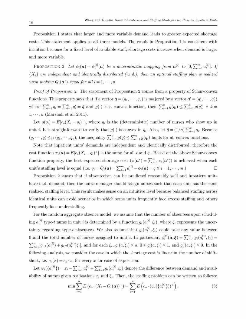
Proposition 1 states that larger and more variable demand leads to greater expected shortage
costs. This statement applies to all three models. The result in Proposition 1 is consistent with
intuition because for a fixed level of available staff, shortage costs increase when demand is larger
and more variable.
Proposition 2. Let φi(a) = φ[d]i (a) be a deterministic mapping from a(i) to [0,
∑m
t=1 a(i)t ]. If
{Xi} are independent and identically distributed (i.i.d.), then an optimal staffing plan is realized
upon making Qi(a∗) equal for all i= 1, · · · , u.
Proof of Proposition 2: The statement of Proposition 2 comes from a property of Schur-convex
functions. This property says that if a vector q = (q1, · · · , qu) is majored by a vector q′ = (q′1, · · · , q′
u)
where∑u
i=1 qi =∑u
i=1 q′
i = ¯q and g(·) is a convex function, then∑k
i=1 g(qi) ≤∑k
i=1 g(q′
i) ∀ k =
1, · · · , u (Marshall et al. 2011).
Let g(qi) = E[co(Xi − qi)+], where qi is the (deterministic) number of nurses who show up in
unit i. It is straightforward to verify that g(·) is convex in qi. Also, let q = (1/u)∑u
i=1 qi. Because
(q, · · · , q)≤M (q1, · · · , qu), the inequality∑u
i=1 g(q)≤∑u
i=1 g(qi) holds for all convex functions.
Note that inpatient units’ demands are independent and identically distributed, therefore the
cost function πi(a) =E[co(Xi− qi)+] is the same for all i and qi. Based on the above Schur-convex
function property, the best expected shortage cost (π(a∗) =∑u
i=1 πi(a∗)) is achieved when each
unit’s staffing level is equal (i.e. qi =Qi(a) =∑m
t=1 a(i)t −φi(a) = q ∀ i=1, · · · ,m.) �
Proposition 2 states that if absenteeism can be predicted reasonably well and inpatient units
have i.i.d. demand, then the nurse manager should assign nurses such that each unit has the same
realized staffing level. This result makes sense on an intuitive level because balanced staffing across
identical units can avoid scenarios in which some units frequently face excess staffing and others
frequently face understaffing.
For the random aggregate absence model, we assume that the number of absentees upon schedul-
ing a(i)t type-t nurse in unit i is determined by a function gt(a
(i)t , ξt), where ξt represents the uncer-
tainty regarding type-t absentees. We also assume that gt(a(i)t , ξt) could take any value between
0 and the total number of nurses assigned to unit i. In particular, φ[r]i (a,ξ) =
∑m
t=1 gt(a(i)t , ξt) =
∑m
t=1[gt,1(a(i)t )+ gt,2(a
(i)t )ξt], and for each ξt, gt(a, ξt)≤ a, 0≤ g′t(a, ξt)≤ 1, and g′′t (a, ξt)≤ 0. In the
following analysis, we consider the case in which the shortage cost is linear in the number of shifts
short, i.e. co(x) = co ·x, for every x for ease of exposition.
Let ψi({a(i)t }) = xi−
∑m
t=1 a(i)t +
∑m
t=1 gt(a(i)t , ξt) denote the difference between demand and avail-
ability of nurses given realizations xi and ξt. Then, the staffing problem can be written as follows:
minu∑
i=1
E(
co · (Xi −Qi(a))+)
=u∑
i=1
E(
co · (ψi({a(i)t }))+
)
, (3)
Wang and Gupta: Nurse Absenteeism and Staffing Strategies for Hospital Inpatient Units19
subject to:u∑
i=1
a(i)t = nt, for each t=1, · · · ,m. (4)
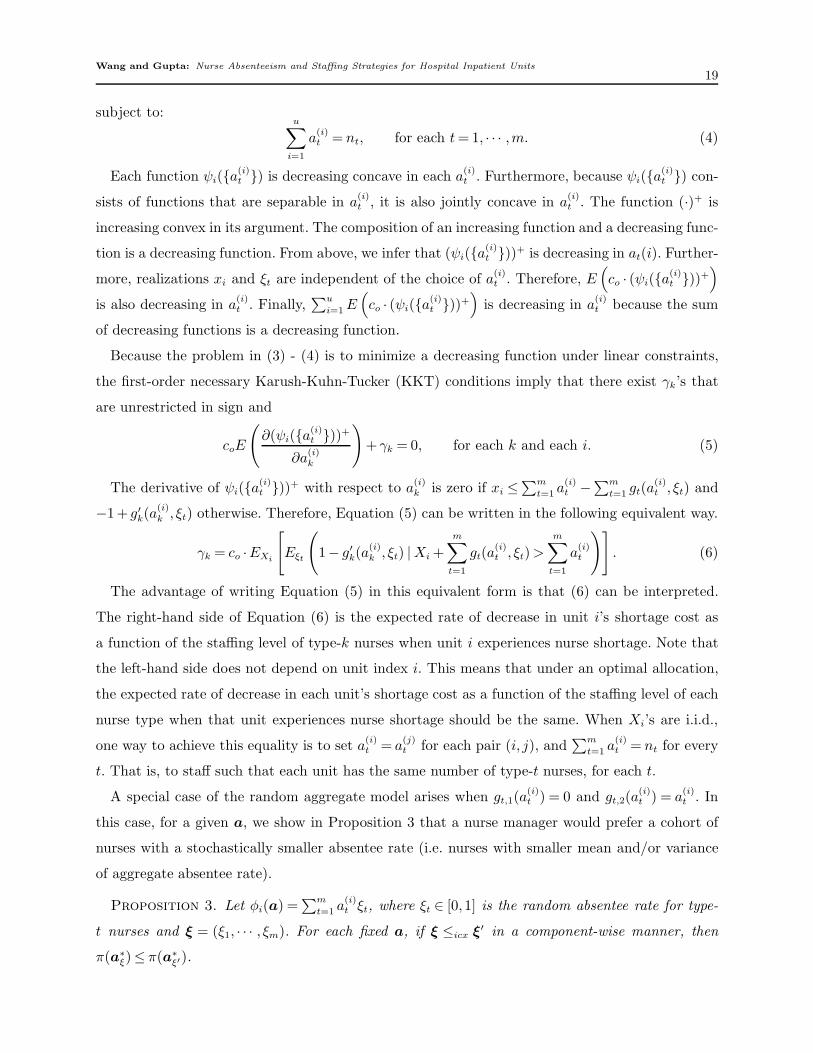
Each function ψi({a(i)t }) is decreasing concave in each a
(i)t . Furthermore, because ψi({a
(i)t }) con-
sists of functions that are separable in a(i)t , it is also jointly concave in a
(i)t . The function (·)+ is
increasing convex in its argument. The composition of an increasing function and a decreasing func-
tion is a decreasing function. From above, we infer that (ψi({a(i)t }))+ is decreasing in at(i). Further-
more, realizations xi and ξt are independent of the choice of a(i)t . Therefore, E
(
co · (ψi({a(i)t }))+
)
is also decreasing in a(i)t . Finally,
∑u
i=1E(
co · (ψi({a(i)t }))+
)
is decreasing in a(i)t because the sum
of decreasing functions is a decreasing function.
Because the problem in (3) - (4) is to minimize a decreasing function under linear constraints,
the first-order necessary Karush-Kuhn-Tucker (KKT) conditions imply that there exist γk’s that
are unrestricted in sign and
coE
(
∂(ψi({a(i)t }))+
∂a(i)k
)
+ γk = 0, for each k and each i. (5)
The derivative of ψi({a(i)t }))+ with respect to a
(i)k is zero if xi ≤
∑m
t=1 a(i)t −
∑m
t=1 gt(a(i)t , ξt) and
−1+ g′k(a(i)k , ξt) otherwise. Therefore, Equation (5) can be written in the following equivalent way.
γk = co ·EXi
[
Eξt
(
1− g′k(a(i)k , ξt) |Xi +
m∑
t=1
gt(a(i)t , ξt)>
m∑
t=1
a(i)t
)]
. (6)
The advantage of writing Equation (5) in this equivalent form is that (6) can be interpreted.
The right-hand side of Equation (6) is the expected rate of decrease in unit i’s shortage cost as
a function of the staffing level of type-k nurses when unit i experiences nurse shortage. Note that
the left-hand side does not depend on unit index i. This means that under an optimal allocation,
the expected rate of decrease in each unit’s shortage cost as a function of the staffing level of each
nurse type when that unit experiences nurse shortage should be the same. When Xi’s are i.i.d.,
one way to achieve this equality is to set a(i)t = a
(j)t for each pair (i, j), and
∑m
t=1 a(i)t = nt for every
t. That is, to staff such that each unit has the same number of type-t nurses, for each t.
A special case of the random aggregate model arises when gt,1(a(i)t ) = 0 and gt,2(a
(i)t ) = a
(i)t . In
this case, for a given a, we show in Proposition 3 that a nurse manager would prefer a cohort of
nurses with a stochastically smaller absentee rate (i.e. nurses with smaller mean and/or variance
of aggregate absentee rate).
Proposition 3. Let φi(a) =∑m
t=1 a(i)t ξt, where ξt ∈ [0,1] is the random absentee rate for type-
t nurses and ξ = (ξ1, · · · , ξm). For each fixed a, if ξ ≤icx ξ′ in a component-wise manner, then
π(a∗
ξ)≤ π(a∗
ξ′).

Wang and Gupta: Nurse Absenteeism and Staffing Strategies for Hospital Inpatient Units20
Proof of Proposition 3: Let π(a) =∑u
i=1 πi(a(i)). Because ξt ≤icx ξ
′
t, πi(a(i)|ξ) = E[co(Xi −
∑m
t=1 a(i)t +
∑m
t=1 a(i)t ξt)
+] ≤ E[co(Xi −∑m
t=1 a(i)t +
∑m
t=1 a(i)t ξ
′
t)+] = πi(a
(i)|ξ′) for each i. Therefore
π(a∗
ξ) = π(a∗
ξ |ξ)≤ π(a∗
ξ′ |ξ)≤ π(a∗
ξ′ |ξ′) = π(a∗
ξ′). �
So far we have shown that a nurse manager prefers smaller and less variable absentee rates. Next,
we address a different question. Given a cohort of heterogeneous nurses, which nurses should a
nurse manager choose to realize less variable absentee rate for his or her unit? We use the concept
of majorization to answer this question. To avoid situations where the manager of each unit would
want only nurses that rarely take unplanned time off, we fix the total aggregate absentee rate that
any choice of nurses must satisfy for that unit. We define p(i) to be the absentee probabilities of
nurses assigned to unit i. That is, components of p(i) contain information about only those nurses
that are assigned to unit i. Furthermore, let πi(p(i)) denote the expected shortage cost incurred
in unit i with no-show probability vector p(i). Then, with individual Bernoulli no-show model, we
can prove that a nurse manager would prefer a more variable mix of absentee rates.
Proposition 4. If p(i) ≤M p′(i), then πi(p′(i))≤ πi(p
(i)).
Proof of Proposition 4: {B(pt), pt ∈ (0,1)} is a family of independent random variables param-
eterized by pt. By Corollary 1 B(pt) is SIL(st). Next, we observe that the function h(b) = x +∑mi
k=1 b(i)k −mi, where x is a realization of random demand Xi, b
(i)k is a realization of B(p
(i)k ), p
(i)k
is the k-th element of vector p(i), and mi is the cardinality of the vector p(i), is an increasing
valuation in b. A function is said to be a valuation if it is both sub- and supermodular (Top-
kis 1998). Define Z(p(i)) = h(B(p(i)1 ), · · · ,B(p(i)mi
)). Then, by Theorem 2, it follows immediately
that {Z(p(i)),p(i) ∈ (0,1)mi} is SI-SchurCX(icx). In addition, for an increasing convex function g,
p(i) ≤M p′(i) implies that E[g(h(B(p′(i)1 ), · · · ,B(p′(i)mi)))]≤ E[g(h(B(p(i)1 ), · · · ,B(p(i)mi
)))]. The state-
ment of the proposition then follows from the fact that co(·) is an increasing convex function.
�
Proposition 4 shows that between two cohorts of nurses that have same head counts and average
group-level absentee rate, the unit’s nurse manager would prefer to utilize the more heterogeneous
cohort of nurses (i.e. the cohort of nurses with more variable absentee probabilities p(i)). However,
this may not be the best overall strategy when costs across different units need to be balanced. In
fact, it is the difficulty of balancing staffing across units while maximizing heterogeneity within a
unit that makes it difficult to identify an optimal assignment strategy.
Next, we show that the results in Propositions 3 and 4 are related. If we view each nurse as
a type, then Corollary 2 establishes that greater heterogeneity within a cohort of nurses leads

Wang and Gupta: Nurse Absenteeism and Staffing Strategies for Hospital Inpatient Units21
to smaller variability in attendance pattern of that cohort taken together, which makes it more
desirable according to Proposition 3.
Corollary 2. Let Bi(p) =∑
n
t=1 a(i)t
B(pt)∑
nt=1 a
(i)t
. If p(i) ≤M p′(i), then Bi(p′)≤icx Bi(p).
Proof of Corollary 2: Recall that p(i) contains only the absentee rates of the mi =∑n
t=1 a(i)t
nurses who are assigned to unit i. Also, the nurse index in vector p(i), which we denote by k,
re-indexes nurses who are assigned to unit i; therefore, it is different from index t.
Following the logic in the proof of Proposition 4, and let h(b) =∑mi
k=1 b(i)k . It is
straightforward to argue that h(b) is an increasing valuation in b. Let Z(p(i)) =∑n
t=1 a(i)t B(p
(i)t ) = h(B(p
(i)1 ), · · · ,B(p(i)mi
)). Then, it can be argued that {Z(p(i)),p(i) ∈ (0,1)mi} is
SI-SchurCX(icx). By Theorem 2, for any increasing convex function g, p(i) ≤M p′(i) implies that
E[g(h(B(p′(i)1 ), · · · ,B(p′(i)mi
)))]≤ E[g(h(B(p(i)1 ), · · · ,B(p(i)mi
)))]. In other words, if p(i) ≤M p′(i), then∑mi
k=1B(p′(i)k ) ≤icx
∑mi
k=1B(p(i)k ), which is equivalent to
∑n
t=1 a(i)t B(p′(i)t ) ≤icx
∑n
t=1 a(i)t B(p
(i)t ). Let
Bi(p) =∑
n
t=1 a(i)t
B(pt)∑
nt=1 a
(i)t
=∑mi
k=1B(p
(i)k
)
mi
be the random proportion of nurses who are absent from work.
Then, from arguments presented above, p(i) ≤M p′(i) also implies Bi(p′)≤icx Bi(p). �
The structural results in Propositions 2-4 and Corollary 2 show that for inpatient units with
identical demand patterns, hospitals’ costs are lower when nurse assignments are as heterogenous
as possible within a unit, but uniform across units. That is, it is desirable to split high absentee
rate nurses across units, and it is desirable to ensure a balanced realized staffing levels when
demand patterns are identical. However, it is not obvious whether simple rules that ensure expected
supply equals expected demand would perform well. Also, solving the model formulated in (1) is
computationally demanding when the number of nurses is large. Therefore, in Section 4, we present
three heuristics that attempt to achieve assignments consistent with the principles identified in
this section.
4. Heuristics and Performance Comparisons
Because the formulation in (1) with nurse-specific Bernoulli representation of absenteeism is a
combinatorially hard problem, we focus in this section on developing implementable heuristics.
To explain the difficulty, consider the fact that for a 12-nurse and 2-unit problem, there are 4096
possible assignments. For each assignment, there are 4096 possible realizations of nurses’ absentee
patterns. To calculate the expected shortage cost, one would need to consider 4096×4096 assign-
ments and nurse attendance combinations for each demand realization. This makes the search for
the optimal nurse assignment difficult for larger-sized problems.

Wang and Gupta: Nurse Absenteeism and Staffing Strategies for Hospital Inpatient Units22
We propose three heuristics in this section, which can be used to obtain assignment of nurses to
inpatient units. We also test these heuristics in numerical experiments. In this section, we allow
multiple nurses to have the same no-show rate. In particular, this means that nt could be greater
than 1 and therefore a(i)t ≤ nt could be greater than 1 as well. Note that this includes the model in
which a(i)t ≤ 1 as a special case. The number of absent nurses in unit i given assignment a can be
expressed by φ[b]i (a) =
∑m
t=1
∑a(i)t
j=1Bj(pt), where Bj(pt) are i.i.d. Bernoulli random variables with
parameter pt. It should be clear that allowing nt ≥ 1 does not result in a loss of generality because
we will obtain the Bernoulli absence model by setting nt = 1.
First, we show that the objective function in (1) is supermodular, which helps to motivate the
heuristics in the sequel. We define δ(i)t (a) = π(a)−π(a+ eti), where eti is a m×u matrix with the
(t, i)-th component equal to 1 and the remaining components equal to 0, as the incremental benefit
of adding a type-t nurse to unit i. Then, it can be shown that
• δ(i)t (a) ≥ 0 ∀ t = 1, · · · ,m, and ∀ i = 1, · · · , u. In addition, when no-show probabilities are
ordered such that p1 ≥ p2 · · · ≥ pm, δ(i)t (a)≤ δ(i)
t′(a) for t≤ t′.
• δ(i)t (a)− δ
(i)t (a+et′i)≥ 0 ∀ t′ = 1, · · · ,m and ∀ i= 1, · · · , u. Note that δ
(i)t (a)− δ
(i)t (a+ et′i) is
the difference in incremental benefits of adding a type-t nurse to unit i under two situations: one
in which this unit had a(i)
t′type-t′ nurses and another in which the number of type-t′ nurses was
a(i)
t′+1.
These results have a straightforward intuitive explanation. The first bullet confirms that it is
better to add a nurse with a lower absentee rate. The second bullet says that the benefit (reduction
in cost) of adding one more type-t nurse to a particular unit diminishes in the number of type-t′
nurses in the unit when the staffing levels of the remaining groups are held constant (note that
t′ is an arbitrary type, which includes t). Together, these observations imply that the objective
function in (1) is supermodular. A more formal argument can be constructed as follows — δ(i)t (a)≥
δ(i)t (a+ et′i) indicates that π(a) + π(a+ et′i + eti)≥ π(a+ et′i) + π(a+ eti). Let x= a+ eti and
y= a+et′i, then we have π(x∨y)+π(x∧y)≥ π(x)+π(y) and π is supermodular.
The reason why supermodularity is relevant is that greedy heuristics have been shown to work
well when the objective function is supermodular; see Il’ev (2001), Calinescu et al. (2011), Asadpour
et al. (2008) for examples of using greedy algorithms for minimizing (reps. maximizing) super-
modular (resp. submodular) functions. Our objective is to minimize a supermodular cost function,
therefore, the nurse manager may wish to sort nurses by increasing absentee rates, and assign them
to different units sequentially to maximize the marginal benefit from each assignment (i.e. in a
greedy fashion) until all nurses are assigned. We call this strategy the greedy assignment. It can
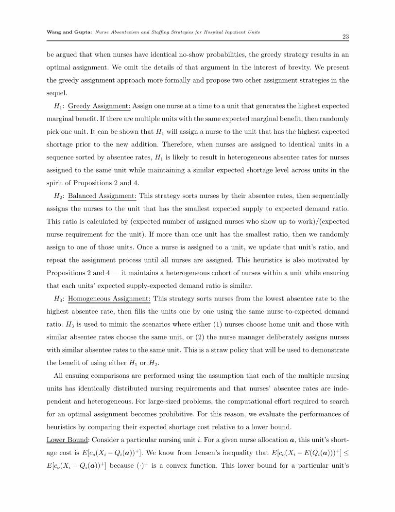
Wang and Gupta: Nurse Absenteeism and Staffing Strategies for Hospital Inpatient Units23
be argued that when nurses have identical no-show probabilities, the greedy strategy results in an
optimal assignment. We omit the details of that argument in the interest of brevity. We present
the greedy assignment approach more formally and propose two other assignment strategies in the
sequel.
H1: Greedy Assignment: Assign one nurse at a time to a unit that generates the highest expected
marginal benefit. If there are multiple units with the same expected marginal benefit, then randomly
pick one unit. It can be shown that H1 will assign a nurse to the unit that has the highest expected
shortage prior to the new addition. Therefore, when nurses are assigned to identical units in a
sequence sorted by absentee rates, H1 is likely to result in heterogeneous absentee rates for nurses
assigned to the same unit while maintaining a similar expected shortage level across units in the
spirit of Propositions 2 and 4.
H2: Balanced Assignment: This strategy sorts nurses by their absentee rates, then sequentially
assigns the nurses to the unit that has the smallest expected supply to expected demand ratio.
This ratio is calculated by (expected number of assigned nurses who show up to work)/(expected
nurse requirement for the unit). If more than one unit has the smallest ratio, then we randomly
assign to one of those units. Once a nurse is assigned to a unit, we update that unit’s ratio, and
repeat the assignment process until all nurses are assigned. This heuristics is also motivated by
Propositions 2 and 4 — it maintains a heterogeneous cohort of nurses within a unit while ensuring
that each units’ expected supply-expected demand ratio is similar.
H3: Homogeneous Assignment: This strategy sorts nurses from the lowest absentee rate to the
highest absentee rate, then fills the units one by one using the same nurse-to-expected demand
ratio. H3 is used to mimic the scenarios where either (1) nurses choose home unit and those with
similar absentee rates choose the same unit, or (2) the nurse manager deliberately assigns nurses
with similar absentee rates to the same unit. This is a straw policy that will be used to demonstrate
the benefit of using either H1 or H2.
All ensuing comparisons are performed using the assumption that each of the multiple nursing
units has identically distributed nursing requirements and that nurses’ absentee rates are inde-
pendent and heterogeneous. For large-sized problems, the computational effort required to search
for an optimal assignment becomes prohibitive. For this reason, we evaluate the performances of
heuristics by comparing their expected shortage cost relative to a lower bound.
Lower Bound: Consider a particular nursing unit i. For a given nurse allocation a, this unit’s short-
age cost is E[co(Xi −Qi(a))+]. We know from Jensen’s inequality that E[co(Xi −E(Qi(a)))
+]≤
E[co(Xi − Qi(a))+] because (·)+ is a convex function. This lower bound for a particular unit’s

Wang and Gupta: Nurse Absenteeism and Staffing Strategies for Hospital Inpatient Units24
shortage cost is dependent on the particular allocation of nurses to this unit through E(Qi(a)).
Next, we derive an allocation-free lower bound.
Let qi =E(Qi(a)) denote the mean number of nurses who show up in unit i given its allocation.
Furthermore∑
iqi = q, where q is the expected number of nurses who will show up for all units.
Then an allocation-free lower bound for the problem in expressions (3)-(4) can be written as follows:
minqi
u∑
i=1
E[co(Xi− qi)+] (7)
subject to∑u
i=1 qi = q and qi ≥ 0. This is a convex minimization problem with linear constraint. It
can be solved easily using KKT first-order necessary conditions (which are also sufficient). The first
order necessary condition states that there exists a γ (unrestricted in sign) such that coFi(qi) = γ for
each i. Therefore, when demand in each unit is i.i.d., it follows that q∗i = q/u. When demand in each
unit does not have the same distribution, then the optimal allocation is achieved at q∗ = (q∗1 , · · · , q∗
u)
such that q∗i = F−1i (γ/co) ∀ i=1, · · · , u and
∑u
i=1 q∗
i = q. In summary, for i.i.d. demand across units,
an allocation-free lower bound is obtained by assigning to each unit an equal proportion of the
mean number of nurses who show up in the cohort of all n nurses and assuming no uncertainty
in nurses’ attendance. Similarly, when inpatient units do not have i.i.d. demand, a lower bound is
obtained by staffing at the same percentile of the demand distributions for each unit such that the
aggregate staffing level sums to the expected number of nurses who will show up.
Next, we present a numerical study to evaluate the three heuristics’ performance relative to this
lower bound using Hospital 1’s staffing data. The examples will show that H1 and H2 consistently
outperform H3, regardless of the size of the problem. Consider a pool of 8u nurses who will be
assigned to u identical units. [Hospital 1’s target staffing level for each telemetry unit was 8 nurses
per shift. This motivated us to pick 8 nurses per unit in a typical shift.] To ensure a balanced
design such that the expected demand equals the expected staffing level, we assume each unit’s
demand follows a Poisson distribution with a mean of λ= 8(1− p), where p is the average absentee
rate for all nurses. We draw 500 random samples of 8u nurses from the pool of nurses who worked
in Hospital 1’s three telemetry units, and calculate each samples’ expected shortage under H1, H2,
H3, and the lower bound for u= 3, · · · ,12. The relative performance for each heuristics reported
in Table 4 is the ratio of its expected shortage cost and the lower bound cost.
H1 and H2 are consistently about 3-4% better than H3 on average. In this numerical example,
over all 3 shifts, a 4% saving for the 4-unit instance will be about $73,052 per year when hourly
shortage cost is calculated as 1.5 times 2012’s nurse mean hourly wage of $32.67 (Bureau of Labor

Wang and Gupta: Nurse Absenteeism and Staffing Strategies for Hospital Inpatient Units25
Table 4 Average Relative Performance
Number of units (u)Heuristics 3 4 5 6 7 8 9 10 11 12
H1 1.0161 1.0166 1.0178 1.0182 1.0187 1.0191 1.0188 1.0196 1.0201 1.0193H2 1.0161 1.0166 1.0178 1.0182 1.0187 1.0191 1.0188 1.0196 1.0201 1.0193H3 1.0429 1.046 1.0519 1.0531 1.0541 1.056 1.0575 1.058 1.0602 1.0591
Statistics 2012). When extrapolated to the entire hospital of a size similar to Hospital 1, savings
could be as high as $1.8-2.4 million per year. To further illustrate the benefit of ensuring a similar
unit-level absentee rate and heterogeneous cohorts of nurses (properties captured by H1 and H2),
we show the percent of cases in which H1 or H2 are better than H3 by x% of the lower bound in
Table 5.
Table 5 Percent of cases in which H1 or H2 is better than H3 by x% of the lower bound
Example 1: i.i.d Demand Across UnitsH1 vs. H3 Number of units (u)
x% 3 4 5 6 7 8 9 10 11 121% 74% 99.2% 100% 99% 100% 100% 100% 100% 100% 100%2% 36.8% 78% 93.2% 83% 88.2% 94.4% 100% 100% 99.8% 100%3% 15% 50.8% 62.8% 53.6% 61.8% 73.6% 97.2% 97.8% 98.4% 96%4% 7.2% 29.6% 38.2% 36.2% 39.8% 50.8% 81.2% 79.8% 81.2% 76.2%5% 4% 17.6% 23.8% 18.6% 24.8% 24.8% 57.6% 54.8% 57.6% 50.6%
H2 vs. H3 Number of units (u)x% 3 4 5 6 7 8 9 10 11 121% 90% 95.6% 99.4% 99.8% 99.6% 100% 99.8% 100% 100% 100%2% 52.8% 65.2% 78.2% 81.2% 88.8% 89.2% 95.4% 95.6% 97% 98.8%3% 30.2% 39% 48.8% 54% 58.6% 62.4% 72.4% 71.2% 79.4% 79.6%4% 16.6% 21.8% 33.8% 31.2% 31.6% 37.2% 43.2% 41.8% 48.6% 49.8%5% 11.4% 12.6% 18.8% 17% 16.8% 20.2% 20.8% 18.2% 23% 20.2%
The results in Table 5 show that the benefit of H1 and H2 as compared to H3 becomes more
significant as the total number of nurses increases because with more nurses, unit-level absentee
rate can be more variable. The results also confirm Propositions 2 and 4 that it is desirable to
utilize heterogeneous cohorts of nurses for individual units while maintaining a similar aggregate
absentee rate among different units.
We also tested the performance of the three heuristics when unit demands were heterogeneous,
but other parameters remained unchanged. In particular, we assumed that roughly 1/3 of the units
had mean demand 0.8λ, 1/3 of the units had mean demand λ, and the remaining one third had
mean demand equal to 1.2λ. When the number of units could not be evenly divided into three
parts, we chose equal first and third cohorts such that the total expected demand and supply
Wang and Gupta: Nurse Absenteeism and Staffing Strategies for Hospital Inpatient Units26
remained balanced. We reached a similar conclusion – H1 and H2 outperformed H3 by 2-5%. We
report the detailed performance comparison for this numerical example in Appendix C.
5. Concluding Remarks
This paper shows that nurse managers may use a nurse’s attendance history to predict his or
her likelihood of being absent in a future shift. This information can be utilized within easy-to-
implement staffing heuristics, e.g. heuristics labeled H1 and H2, to reduce staffing costs. The use
of such heuristics does not require much effort on part of nurse managers.
The contribution of this paper lies in (1) developing detailed analyses of data from multiple
inpatient units to identify observable predictors of nurse absenteeism, (2) establishing structural
properties of optimal assignment strategies, and (3) developing and testing easy-to-implement
heuristics for use by nurse managers. The structural properties we establish provide insights for
developing staffing strategies in environments where work is performed by teams of employees.
The savings are of the order of 3-4% of overtime costs, which may be considered small by some.
However, it is important to note that our approach reduces variance in attendance rate and that
the approach is easy to implement. Therefore, nurse managers do not need to exert much effort to
realize the benefit of reduced cost and reduced day-to-day variability in the number of additional
nurses they will need to find to meet requirements in each shift. In addition, the proposed strategies
utilize information that is easy to track from historical data – nurses’ absentee rates and inpatient
units’ demand distributions. The former may be estimated from nurses’ attendance records whereas
the latter may be estimated from census data and target nurse-to-patient ratios.
A limitation of our mathematical model comes from an implicit assumption that nurses’ absentee
rates will remain unchanged with re-assignments. Many hospital environments are highly dynamic,
and nurses’ absenteeism may be affected by unit-specific norms, management style, and esprit de
corps. Whereas behavioral factors and people management skills are important in hospital setting,
such factors are beyond the scope of this paper. Many papers in the HSR literature discuss possible
strategies to mitigate such operational challenges. See Seago and Faucett (1997), Fletcher (2001),
Andrews and Dziegielewski (2005), San Park and Kim (2009), for further information.
References
Aiken, L. H., S. P. Clarke, D. M. Sloane, J. Sochalski, J. H. Siber. 2002. Hospital nurse staffing and patient
mortality, nurse burnout and job dissatisfaction. The Journal of the American Medical Association
288(16) 1987 – 1993.
Andrews, D. R., S. F. Dziegielewski. 2005. The nurse manager: job satisfaction, the nursing shortage and
retention. Journal of Nursing Management 13(4) 286–295.

Wang and Gupta: Nurse Absenteeism and Staffing Strategies for Hospital Inpatient Units27
Anonymous. 2010. 2010 Emergency Department Pulse Report – Patient Perspectives on American Health
Care. Available at: http://goo.gl/vz4eI, downloaded 1/31/2012.
Araman, V. F., I. Popescu. 2010. Media revenue management with audience uncertainty: Balancing upfront
and spot market sales. Manufacturing & Service Operations Management 12(2) 190–212.
Asadpour, A., H. Nazerzadeh, A. Saberi. 2008. Stochastic submodular maximization. Internet and Network
Economics . Springer, 477–489.
Bell, M. L., K. Ebisu, R. D. Peng, J. Walker, J. M. Samet, S. L. Zeger, F. Dominici. 2008. Seasonal
and regional short-term effects of fine particles on hospital admissions in 202 us counties, 1999-2005.
American Journal of Epidemiology 168(11) 1301–1310.
Birge, J. R., F. Louveaux. 2011. Introduction to stochastic programming. 2nd ed. Springer New York; Berlin;
Heidelberg. SpringerLink (Online service).
Blumenfeld, D. E., R. R. Inman. 2009. Impact of absenteeism on assembly line quality and throughput.
Production and Operations Managment 18(3) 333–343.
Bollapragada, S., T. E. Morton. 1999. Myopic heuristics for the random yield problem. Operations Research
47(5) 713–722.
Bureau of Labor Statistics. 2011. Household data annual averages. Current Population Survey Abailable at:
http://www.bls.gov/cps/cpsaat47.pdf.
Bureau of Labor Statistics. 2012. Occupational employment and wages for registered nurses. Occupational
Employment Statistics Abailable at: http://www.bls.gov/cps/cpsaat47.pdf.
California Nurse Association, National Nurses Organizing Committee. 2012. Floating according to the rules.
Nursing Practice & Patient Advocacy Alert Available at http://goo.gl/nMqcp, downloaded 4/19/2012.
Calinescu, G., C. Chekuri, M. Pal, J. Vondrak. 2011. Maximizing a monotone submodular function subject
to a matroid constraint. SIAM Journal on Computing 40(6) 1740–1766.
Cho, S-H, S. Ketefian, V. H. Barkauskas, D. G. Smith. 2003. The effects of nurse staffing on adverse events,
morbidity, mortality, and medical costs. Nursing Research 52(2) 71 – 79.
Ciarallo, F. W., R. Akella, T. E. Morton. 1994. A periodic review, production planning model with uncertain
capacity and uncertain demandoptimality of extended myopic policies. Management Science 40 320 –
332.
Davey, M. M., G. Cummings, C. V. Newburn-Cook, E. A. Lo. 2009. Predictors of nurse absenteeism in
hospitals: a systematic review. Journal of nursing management 17(3) 312–30.
Ferlise, P., D. Baggot. 2009. Improving staff nurse satisfaction and nurse turnover: use of a closed-unit
staffing model. Journal of Nursing Administration 39(7/8) 318–320.
Fletcher, C. E. 2001. Hospital rns’ job satisfactions and dissatisfactions. Journal of Nursing Administration
31(6) 324–331.

Wang and Gupta: Nurse Absenteeism and Staffing Strategies for Hospital Inpatient Units28
Gerchak, Y., R. G. Vickson, M. Parlar. 1988. Periodic review production models with variable yield and
uncertain demand? IIE transactions 20(2) 144–150.
Green, L. V., S. Savin, N. Savva. 2013. “nursevendor problem”: Personnel staffing in the presence of endoge-
nous absenteeism. Management Science doi:10.1287/mnsc.2013.1713.
Grosfeld-Nir, A., Y. Gerchak. 2004. Multiple lotsizing in production to order with random yields: Review of
recent advances. Annals of Operations Research 126(1-4) 43–69.
Grosfeld-Nir, A., Y. Gerchak, Q.-M. He. 2000. Manufacturing to order with random yield and costly inspec-
tion. Operations Research 48(5) 761 – 767.
Gurnani, H., R. Akella, J. Lehoczky. 2000. Supply management in assembly systems with random yield and
random demand. IIE Transactions 32(8) 701–714.
Hur, D., V. A. Mabert, K. M. Bretthauer. 2004. Real-time work schedule adjustment decisions: An investi-
gation and evaluation. Production and Operations Management 13(4) 322–339.
Il’ev, V. P. 2001. An approximation guarantee of the greedy descent algorithm for minimizing a supermodular
set function. Discrete Applied Mathematics 114(1) 131–146.
Kane, R. L., T. A. Shamliyan, C. Mueller, S. Duval, T. J. Wilt. 2007. The association of registered nurse
staffing levels and patient outcomes. systematic review and meta-analysis. Medical Care 45(12) 1195
– 1204.
Ken, F. 2006. ‘Patient’ says it all. USA Today Available at http://goo.gl/nMqcp, downloaded 1/31/2012.
Lang, T. A., M. Hodge, V. Olson, P. S. Romano, R. L. Kravitz. 2004. Nurse–patient ratios: A systematic
review on the effects of nurse staffing on patient, nurse employee, and hospital outcomes. The Journal
of Nursing Administration 34(7-8) 326 – 337.
Laschinger, H.K.S., A. L. Grau. 2012. The influence of personal dispositional factors and organizational
resources on workplace violence, burnout, and health outcomes in new graduate nurses: A cross-sectional
study. International Journal of Nursing Studies 49(3) 282 – 291.
Lim, G. J., A. Mobasher, L. Kardar, M. J. Cote. 2011. Nurse scheduling. R. W. Hall, ed., Handbook of
Healthcare System Scheduling: Deliverying Care When and Where It is Needed , chap. 3. Springer, NY,
31 – 64.
Liyanage, L., J. G. Shanthikumar. 1992. Allocation through stochastic schur convexity and stochastic trans-
position increasingness. Lecture Notes-Monograph Series 22 pp. 253–273.
Marshall, A. W., I. Olkin, B. C. Arnold. 2011. Inequalities: Theory of Majorization and Its Applications .
2nd ed. Springer, NY.
National Center for Health Statistics. 2011. Health, United States, 2010: With Special Feature on Death
and Dying. Available at http://www.cdc.gov/nchs/data/hus/hus10.pdf, downloaded 1/31/2012.

Wang and Gupta: Nurse Absenteeism and Staffing Strategies for Hospital Inpatient Units29
National Climatic Data Center. 2012. NCDC Storm Event Database. Data available at http://goo.gl/V3zWs,
downloaded 1/12/2012.
Needleman, J., P. Buerhaus, S. Mattke, M. Stewart, K. Zelevinsky. 2002. Nurse-staffing levels and the quality
of care in hospitals. The New England Journal of Medicine 346(22) 1715 – 1722.
Rajbhandary, S., K. Basu. 2010. Working conditions of nurses and absenteeism: Is there a relationship? an
empirical analysis using national survey of the work and health of nurses. Health Policy 97(2-3) 152 –
159.
Roelen, C.A.M., P.C. Koopmans, J.A.H. Schreuder, J.R. Anema, A.J. van der Beek. 2011. The history of
registered sickness absence predicts future sickness absence. Occupational medicine 61(2) 96–101.
San Park, J., T. H. Kim. 2009. Do types of organizational culture matter in nurse job satisfaction and
turnover intention? Leadership in Health Services 22(1) 20–38.
Schreuder, J., C. Roelen, N. van Zweeden, D. Jongsma, J. van der Klink, J. Groothoff. 2011. Leadership styles
of nurse managers and registered sickness absence among their nursing staff. Health care management
review 36(1) 58–66.
Seago, J. A., J. Faucett. 1997. Job strain among registered nurses and other hospital workers. Journal of
Nursing Administration 27(5) 19–25.
Shaked, M., J. G. Shanthikumar. 2007. Stochastic orders . New York : Springer.
Sochalski, J., L. H. Aiken, C Fagin. 1997. Hospital restructuring in the United States, Canada, and Western
Europe: an outcomes research agenda. Midical Care 35(10) 13–25.
Sovie, M.D., A.F. Jawad. 2001. Hospital restructuring and its impact on outcomes: nursing staff regulations
are premature. The Journal of nursing administration 31(12) 588–600.
Topkis, D. 1998. Supermodularity and complementarity. 2nd ed. Princeton University Press, New Jersey.
Unruh, L. 2008. Nurse staffing and patient, nurse, and financial outcomes. American Journal of Nursing
108(1) 62–71.
Whitt, W. 2006. Staffing a call center with uncertain arrival rate and absenteeism. Production and Operations
Management 15(1) 88–102.
Yano, C. A., H. L. Lee. 1995. Lot sizing with random yields: A review. Operations Research 43(2) pp.
311–334.

Wang and Gupta: Nurse Absenteeism and Staffing Strategies for Hospital Inpatient Units30
Appendix. A
Table 6 Fiscal year 2009 statistics for the two hospitals.
Hospital 1 Hospital 2Size/VolumeAvailable beds 466 284Maximum Daily Census 359 242Minimum Daily Census 205 149Average Daily Census 292 188Admissions 30,748 14,851Patient Days 114,591 68,924Admissions through ER 14,205 6,019Acute Care Admissions 26,751 13,694Acute Patient Days 106,625 66,842Average Acute Care Length of Stay (days) 4.0 4.9Number of RN FTEs 855.9 415.4Expenses/Income (in millions)RN salary expenses $73.2 $36.6Total Operating Revenue $431.2 $231,4Total Operating Expenses $408.5 $235.5Total Operating Income $22.7 $-4.1Available beds = number of beds immediately available for use.
RN = registered nurse. FTE = full-time equivalent.
Table 7 Number of patients per nurse by shift type.
Shift Type TR Unit Mean SD 95% CIWeekday 3 T1 2.98 0.60 (2.92, 3.03)Day & 3 T2 3.25 0.63 (3.20, 3,31)Evening shifts 3 T3 2.81 0.81 (2.73, 2.88)Weekends 4 T1 3.85 1.04 (3.76, 3.94)and 4 T2 3.77 1.29 (3.66, 3.88)Night shifts 4 T3 3.04 0.67 (2.98, 3.09)
Day & 4 M1 2.99 0.56 (2.95, 3.03)Evening Shifts 4 M2 3.14 0.39 (3.12, 3.17)Night 5 M1 4.97 1.07 (4.90, 5.05)Shifts 5 M2 5.21 0.80 (5.15, 5.27)TR = target number of patients per nurse
SD = standard deviation. CI = confidence interval.

Wang and Gupta: Nurse Absenteeism and Staffing Strategies for Hospital Inpatient Units31
Table 8 Absentee Rate by Unit, Day of Week (DoW), Shift, Holidays, and Storm Days.
Hospital 1Unit Mean SD 95% CIT1 0.101 0.134 (0.093, 0.109)T2 0.082 0.111 (0.075, 0.089)T3 0.067 0.091 (0.061, 0.073)
DoW Mean SD 95% CISun 0.077 0.118 (0.066, 0.089)Mon 0.093 0.124 (0.081, 0.104)Tue 0.077 0.103 (0.068, 0.087)Wed 0.074 0.100 (0.065, 0.083)Thu 0.086 0.111 (0.075, 0.096)Fri 0.088 0.116 (0.077, 0.099)Sat 0.086 0.123 (0.074, 0.098)
Shift Mean SD 95% CIDay 0.058 0.090 (0.053, 0.064)
Evening 0.085 0.096 (0.079, 0.091)Night 0.107 0.143 (0.098, 0.116)
Day 12-hour 0.134 0.341 (0.112, 0.156)Night 12-hour 0.228 0.420 (0.201, 0.256)
Holidaya Mean SD 95% CINon holiday 0.083 0.113 (0.079, 0.087)Holidays 0.084 0.138 (0.054, 0.114)
Storm Daysb Mean SD 95% CINo 0.082 0.114 (0.078, 0.087)Yes 0.129 0.149 (0.088, 0.171)
Hospital 2Unit Mean SD 95% CIM1 0.062 0.104 (0.057, 0.068)M2 0.091 0.118 (0.085, 0.098)– – – –
DoW Mean SD 95% CISun 0.076 0.112 (0.065, 0.087)Mon 0.082 0.120 (0.071, 0.094)Tue 0.084 0.120 (0.072, 0.095)Wed 0.072 0.108 (0.062, 0.083)Thu 0.077 0.112 (0.066, 0.087)Fri 0.073 0.102 (0.063, 0.083)Sat 0.075 0.107 (0.064, 0.085)
Shift Mean SD 95% CIDay 0.057 0.083 (0.051, 0.063)
Evening 0.075 0.098 (0.067, 0.082)Night 0.088 0.129 (0.079, 0.097)– – – –– – – –
Holidaysa Mean SD 95% CINon holiday 0.078 0.112 (0.074, 0.082)Holiday 0.051 0.101 (0.032, 0.070)
Storm Daysb Mean SD 95% CINo 0.077 0.112 (0.073, 0.081)Yes 0.10 0.126 (0.052, 0.143)
aHolidays include US federal holidays and the day before Thanksgiving and Christmas.bStorm days were 2/26/09, 5/5/09, 8/2/09, 8/8/09, 10/12/09, 12/8/09, and 12/23/09 according to
National Climatic Data Center (2012).
SD = Standard Deviation. CI = Confidence Interval.

Wang and Gupta: Nurse Absenteeism and Staffing Strategies for Hospital Inpatient Units32
Appendix. B
B.1. Unit-Pooled Model
Table 9 Result of the Statistical Model With Unit and Nurse As Nested Random Effects by w(k)it
k= 1 k= 2 k= 3Random Effect: Standard Deviation Standard Deviation Standard DeviationNurse:Unit (Intercept) 0.751 0.752 0.743Unit (Intercept) 0.244 0.200 0.112Fixed Effects: Est. S.E. Pr(> |z|) Est. S.E. Pr(> |z|) Est. S.E. Pr(> |z|)(Intercept) -2.675 0.1964 <0.001∗ -2.698 0.180 <0.001∗ -2.724 0.154 <0.001∗
ShiftE 0.298 0.1204 0.013∗ 0.361 0.117 0.002∗ 0.406 0.116 <0.001∗
ShiftN 0.517 0.1383 <0.001∗ 0.497 0.139 <0.001∗ 0.475 0.139 0.001∗
ShiftD12 -0.111 0.2128 0.602 -0.131 0.222 0.555 0.397 0.191 0.038∗
ShiftE12 0.261 0.2029 0.198 0.349 0.189 0.065 0.727 0.166 <0.001∗
w(1)t 0.010 0.0028 0.001∗ -0.009 0.003 0.002∗ -0.013 0.005 0.006∗
MonthFeb -0.035 0.1311 0.791 0.004 0.131 0.974 0.040 0.131 0.763MonthMar -0.239 0.1348 0.076 -0.204 0.135 0.131 -0.191 0.135 0.158MonthApr -0.194 0.1326 0.143 -0.156 0.132 0.238 -0.112 0.133 0.402MonthMay -0.246 0.1381 0.075 -0.218 0.138 0.114 -0.219 0.138 0.113MonthJun -0.219 0.1361 0.107 -0.148 0.136 0.277 -0.103 0.138 0.455MonthJul -0.089 0.1363 0.512 -0.099 0.137 0.469 -0.097 0.136 0.476MonthAug -0.151 0.1344 0.260 -0.131 0.134 0.330 -0.130 0.134 0.331MonthSep -0.365 0.1420 0.010∗ -0.332 0.142 0.019∗ -0.330 0.142 0.020∗
MonthOct 0.281 0.1227 0.022∗ 0.358 0.122 0.003∗ 0.432 0.124 <0.001∗
MonthNov -0.173 0.1328 0.194 -0.094 0.132 0.476 -0.016 0.132 0.902MonthDec -0.707 0.3021 0.019∗ -0.614 0.301 0.042∗ -0.504 0.303 0.096Holiday 0.116 0.1860 0.534 0.069 0.186 0.710 0.003 0.187 0.988Weather 0.274 0.2085 0.189∗ 0.293 0.208 0.160 0.327 0.207 0.114
ShiftE:w(k)it -0.001 0.0034 0.705 0.003 0.004 0.382 0.004 0.006 0.480
ShiftN:w(k)it -0.008 0.0034 0.017∗ 0.009 0.003 0.005∗ -0.003 0.006 0.674
ShiftD12:w(k)it 0.027 0.0058 <0.001∗ -0.034 0.008 <0.001∗ 0.020 0.017 0.249
ShiftE12:w(k)it 0.009 0.0049 0.081 -0.015 0.006 0.008∗ 0.000 0.008 0.967
Standard Deviation: Standard deviation of the random intercepts.Est.: Estimate, S.E.: Standard Error of the Estimate, P (> |z|): p-value of Wald statistics.∗: Significant at 0.05 level.
For workload models 2 and 3, we varied m (the moving average parameter) between 4 and 10 and the
conclusion from the statistical analysis remains the same. We report the results for m = 6 for the sake of
brevity. The results show that individual nurses’ random effect is strong (see the large standard deviation of
the random intercept due to nurse heterogeneity) as compared to the fixed effects. The unit random effect
may exist but its impact is not as high as the shift fixed effect and the random nurse effect.

Wang and Gupta: Nurse Absenteeism and Staffing Strategies for Hospital Inpatient Units33
B.2. Unit-Specific Model
Table 10 Result of the Statistical Model When Workload is Evaluated by w(2)it
Unit T1 T2 T3Rndom Effect: Standard Deviation Standard Deviation Standard DeviationNurse (Intercept) 0.877 0.626 0.657Fixed Effects: Est. S.E. P (> |z|) Est. S.E. P (> |z|) Est. S.E. P (> |z|)(Intercept) -2.553 0.261 <0.001∗ -2.500 0.217 <0.001∗ -3.395 0.302 <0.001∗
ShiftE 0.102 0.233 0.661 0.442 0.171 0.010∗ 0.720 0.286 0.012ShiftN 0.866 0.286 0.002∗ 0.436 0.209 0.037∗ 0.631 0.317 0.046∗
ShiftD12 0.399 0.623 0.522 0.455 0.273 0.096 -1.438 0.615 0.019∗
ShiftN12 0.495 0.695 0.476 0.492 0.249 0.048∗ 0.205 0.419 0.624
w(2)it -0.003 0.005 0.560 -0.007 0.004 0.079 -0.023 0.008 0.004∗
MonthFeb -0.022 0.234 0.926 -0.019 0.227 0.935 0.050 0.227 0.825MonthMar -0.365 0.242 0.133 -0.078 0.229 0.732 -0.175 0.236 0.459MonthApr -0.040 0.227 0.859 -0.424 0.247 0.087 -0.074 0.229 0.746MonthMay -0.213 0.236 0.368 -0.212 0.242 0.380 -0.289 0.255 0.258MonthJun -0.183 0.236 0.438 -0.170 0.244 0.486 -0.151 0.238 0.524MonthJul -0.571 0.257 0.026∗ -0.064 0.241 0.790 0.212 0.225 0.347MonthAug -0.504 0.253 0.046 0.092 0.233 0.692 -0.068 0.226 0.765MonthSep -0.436 0.247 0.078 -0.503 0.268 0.060 -0.183 0.238 0.443MonthOct 0.175 0.220 0.427 0.345 0.214 0.107 0.482 0.207 0.020∗
MonthNov -0.307 0.236 0.194 -0.005 0.232 0.981 -0.081 0.227 0.721MonthDec -1.133 0.570 0.047∗ -0.029 0.439 0.947 -0.847 0.619 0.171Holiday -0.113 0.357 0.752 -0.136 0.327 0.677 0.507 0.299 0.090Weather 0.702 0.327 0.032∗ 0.399 0.371 0.281 -0.404 0.450 0.370
ShiftE:w(2)it -0.004 0.007 0.553 0.008 0.005 0.133 0.009 0.009 0.299
ShiftN:w(2)it 0.007 0.006 0.216 0.001 0.005 0.834 0.012 0.009 0.191
ShiftD12:w(2)it -0.050 0.033 0.137 -0.042 0.012 0.001∗ -0.057 0.018 0.002∗
ShiftN12:w(2)it -0.065 0.026 0.014∗ -0.010 0.008 0.183 -0.009 0.013 0.501
Standard Deviation: Standard deviation of the random intercepts.Est.: Estimate, S.E.: Standard Error of the Estimate, P (> |z|): p-value of Wald statistics.∗: Significant at 0.05 level.

Wang and Gupta: Nurse Absenteeism and Staffing Strategies for Hospital Inpatient Units34
Table 11 Result of the Statistical Model When Workload is Evaluated by w(3)it
Unit T1 T2 T3Rndom Effect: Standard Deviation Standard Deviation Standard DeviationNurse (Intercept) 0.873 0.617 0.649Fixed Effects: Est. S.E. P (> |z|) Est. S.E. P (> |z|) Est. S.E. P (> |z|)(Intercept) -2.702 0.269 <0.001∗ -2.518 0.229 <0.001∗ -3.031 0.237 <0.001∗
ShiftE 0.277 0.235 0.238 0.475 0.180 0.008∗ 0.503 0.198 0.011∗
ShiftN 1.016 0.285 <0.001∗ 0.379 0.213 0.075 0.264 0.241 0.274ShiftD12 1.366 0.597 0.022∗ 0.402 0.290 0.166 0.289 0.277 0.297ShiftN12 2.125 0.441 <0.001∗ 0.582 0.251 0.021∗ 0.436 0.273 0.110
w(3)it -0.015 0.008 0.048∗ -0.005 0.008 0.519 -0.023 0.010 0.026∗
MonthFeb <0.001 0.233 0.999 -0.034 0.228 0.883 0.167 0.228 0.463MonthMar -0.321 0.242 0.184 -0.109 0.229 0.636 -0.152 0.237 0.521MonthApr 0.061 0.225 0.787 -0.448 0.249 0.072 -0.001 0.231 0.998MonthMay -0.146 0.235 0.536 -0.253 0.241 0.293 -0.344 0.255 0.177MonthJun -0.083 0.237 0.726 -0.192 0.247 0.435 -0.042 0.241 0.862MonthJul -0.425 0.255 0.095 -0.035 0.235 0.882 0.174 0.225 0.440MonthAug -0.536 0.255 0.035 0.041 0.232 0.860 0.051 0.226 0.823MonthSep -0.393 0.246 0.110 -0.556 0.267 0.037∗ -0.118 0.238 0.621MonthOct 0.278 0.221 0.210 0.365 0.217 0.093 0.648 0.210 0.002∗
MonthNov -0.199 0.234 0.394 0.001 0.233 0.997 0.142 0.227 0.531MonthDec -1.028 0.574 0.073∗ 0.003 0.439 0.995 -0.590 0.622 0.343Holiday -0.247 0.364 0.498 -0.152 0.325 0.640 0.379 0.297 0.203Weather 0.791 0.326 0.015∗ 0.417 0.365 0.252 -0.410 0.451 0.363
ShiftE:w(3)it 0.009 0.010 0.353 0.003 0.011 0.818 0.007 0.012 0.531
ShiftN:w(3)it -0.001 0.010 0.925 0.002 0.012 0.849 -0.011 0.014 0.436
ShiftD12:w(3)it 0.097 0.073 0.183 -0.002 0.020 0.927 0.048 0.031 0.117
ShiftN12:w(3)it -0.022 0.021 0.316 0.001 0.013 0.932 0.004 0.015 0.785
Standard Deviation: Standard deviation of the random intercepts.Est.: Estimate, S.E.: Standard Error of the Estimate, P (> |z|): p-value of Wald statistics.∗: Significant at 0.05 level.
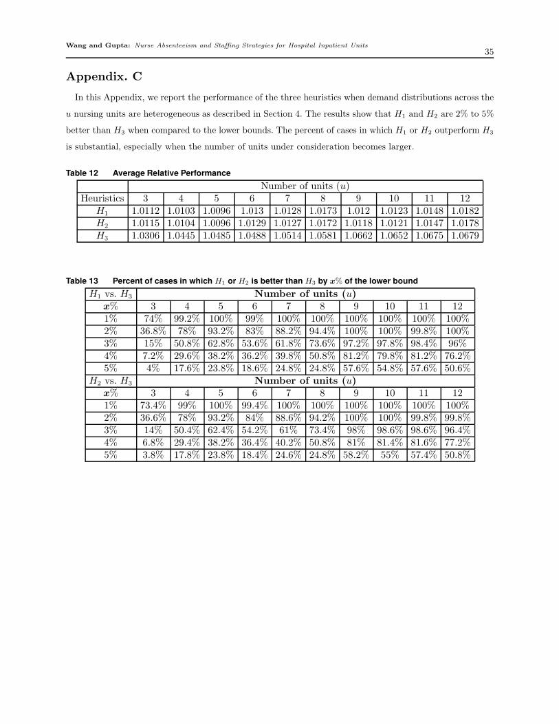
Wang and Gupta: Nurse Absenteeism and Staffing Strategies for Hospital Inpatient Units35
Appendix. C
In this Appendix, we report the performance of the three heuristics when demand distributions across the
u nursing units are heterogeneous as described in Section 4. The results show that H1 and H2 are 2% to 5%
better than H3 when compared to the lower bounds. The percent of cases in which H1 or H2 outperform H3
is substantial, especially when the number of units under consideration becomes larger.
Table 12 Average Relative Performance
Number of units (u)Heuristics 3 4 5 6 7 8 9 10 11 12
H1 1.0112 1.0103 1.0096 1.013 1.0128 1.0173 1.012 1.0123 1.0148 1.0182H2 1.0115 1.0104 1.0096 1.0129 1.0127 1.0172 1.0118 1.0121 1.0147 1.0178H3 1.0306 1.0445 1.0485 1.0488 1.0514 1.0581 1.0662 1.0652 1.0675 1.0679
Table 13 Percent of cases in which H1 or H2 is better than H3 by x% of the lower bound
H1 vs. H3 Number of units (u)x% 3 4 5 6 7 8 9 10 11 121% 74% 99.2% 100% 99% 100% 100% 100% 100% 100% 100%2% 36.8% 78% 93.2% 83% 88.2% 94.4% 100% 100% 99.8% 100%3% 15% 50.8% 62.8% 53.6% 61.8% 73.6% 97.2% 97.8% 98.4% 96%4% 7.2% 29.6% 38.2% 36.2% 39.8% 50.8% 81.2% 79.8% 81.2% 76.2%5% 4% 17.6% 23.8% 18.6% 24.8% 24.8% 57.6% 54.8% 57.6% 50.6%
H2 vs. H3 Number of units (u)x% 3 4 5 6 7 8 9 10 11 121% 73.4% 99% 100% 99.4% 100% 100% 100% 100% 100% 100%2% 36.6% 78% 93.2% 84% 88.6% 94.2% 100% 100% 99.8% 99.8%3% 14% 50.4% 62.4% 54.2% 61% 73.4% 98% 98.6% 98.6% 96.4%4% 6.8% 29.4% 38.2% 36.4% 40.2% 50.8% 81% 81.4% 81.6% 77.2%5% 3.8% 17.8% 23.8% 18.4% 24.6% 24.8% 58.2% 55% 57.4% 50.8%