stability derivative extraction - digital...
TRANSCRIPT
AIRCRAFT STABILITY DERIVATIVE
ESTIMATION FROM FINITE
ELEMENT ANALYSIS
By
DERIC AUSTIN BABCOCK
Bachelor of Science
Oklahoma State University
Stillwater, Oklahoma
2002
Submitted to the Faculty of the Graduate College of Oklahoma State University
in partial fulfillment of the requirements for
the Degree of MASTER OF SCIENCE
July, 2004

ii
AIRCRAFT STABILITY DERIVATIVE
ESTIMATION FROM FINITE
ELEMENT ANALYSIS
Thesis Approved:
____________________Dr. Arena____________________
Thesis Advisor
_____________________Dr. Falk_____________________
____________________Dr. Young____________________
___________________Dr. Carlozzi___________________ Dean of the Graduate College

iii
ACKNOWLEDGEMENTS
First, I would like to thank my wife, Caitlin, for her love and support throughout
this entire process. Her patience, comfort, and encouragement made this work possible.
I would also like to thank my mother, Sandy, for teaching me the importance of
education and the rewards of hard work. I am astonished that you were able to raise
Shane and me while working three jobs and pursuing higher education.
I would like to thank Dr. Arena for his guidance and input into my thesis. He
encouraged me not to settle for a sub-par performance and helped me focus on the
research objective. I also want to thank Dr. Arena, as well as the NASA Oklahoma
Space Grant, for funding my research. I am greatly thankful for the F-18 surface model
provided by NASA Dryden, so I would especially like to thank Tim Doyle, Ed Hahn, and
Dr. Gupta.
Finally, I would like to thank all who have worked in the CASE Lab for helping
lay the foundations upon which my work is based, and especially those who have been
helpful during the course of this work: Anthony Boeckman, Nic Moffitt, and Charles
ONeill. Thank you all.

iv
TABLE OF CONTENTS
Chapter Page
1 INTRODUCTION ........................................................................................................... 1
1.1 Background......................................................................................................... 1 1.2 Motivation........................................................................................................... 4 1.3 Objective............................................................................................................. 6
2 LITERATURE REVIEW ................................................................................................ 8
2.1 Flow Solvers ....................................................................................................... 8 2.1.1 General Requirements..................................................................................... 8 2.1.2 Panel Methods............................................................................................... 10 2.1.3 STARS .......................................................................................................... 11 2.1.4 Piston-Perturbation Solver ............................................................................ 12
2.2 Excitation Signals ............................................................................................. 13 2.2.1 Signal Requirements ..................................................................................... 13 2.2.2 Signal Characteristics.................................................................................... 16 2.2.3 3211 Multistep .............................................................................................. 16 2.2.4 Chirp ............................................................................................................. 17 2.2.5 DC-Chirp....................................................................................................... 19 2.2.6 Other Signals................................................................................................. 20
2.3 Model Formulations.......................................................................................... 21 2.3.1 Rigid Body Equations of Motion.................................................................. 22 2.3.2 Indicial Functions.......................................................................................... 23 2.3.3 ARMA Model ............................................................................................... 25 2.3.4 Nonlinear Model: Stepwise Regression....................................................... 26
2.4 Parameter Estimation Methods......................................................................... 27 2.4.1 Maximum Likelihood Estimation................................................................. 28 2.4.2 Output Error Method..................................................................................... 28 2.4.3 Equation Error Method ................................................................................. 29
3 METHODOLOGY ........................................................................................................ 30
3.1 Forced Oscillation Parameter Identification ..................................................... 30 3.1.1 CFD Solver ................................................................................................... 31 3.1.2 Input Excitation............................................................................................. 33 3.1.3 Parameter Identification................................................................................ 38 3.1.4 Extracting Stability Derivatives.................................................................... 40
3.2 Decoupled Boundary Conditions...................................................................... 42

v
3.2.1 Deriving Equations ....................................................................................... 44 3.2.2 Non-Inertial Boundary Condition Equation.................................................. 45 3.2.3 Theodorsens Moment Equation................................................................... 46
4 RESULTS AND DISCUSSION.................................................................................... 50
4.1 Forced Oscillation Parameter Identification ..................................................... 50 4.1.1 Horizontal Tail .............................................................................................. 50 4.1.2 Dihedral Wing............................................................................................... 62
4.2 Decoupled Boundary Condition Specification ................................................. 69 4.2.1 Airfoil............................................................................................................ 70 4.2.2 Horizontal Tail .............................................................................................. 76 4.2.3 Dihedral Wing............................................................................................... 82 4.2.4 Simple Aircraft.............................................................................................. 85 4.2.5 F-18A ............................................................................................................ 88
5 CONCLUSIONS AND RECOMMENDATIONS ...................................................... 100
5.1 Conclusions..................................................................................................... 100 5.2 Recommendations........................................................................................... 101
BIBLIOGRAPHY........................................................................................................... 103
APPENDIX A: THIN AIRFOIL THEORY FOR CONSTANT PITCH RATE ............ 107
APPENDIX B: DATCOM CALCULATIONS FOR ISOLATED SURFACES ........... 109
APPENDIX C: DATCOM CALCULATIONS INCLUDING INTERFERENCE ........ 114

vi
LIST OF FIGURES
Figure 1.1: Illustration of Static Stability .......................................................................... 2 Figure 1.2: Illustration of Dynamic Stability..................................................................... 3 Figure 2.1: 3211 Multistep Applied to Velocity.............................................................. 16 Figure 2.2: Chirp Excitation Signal ................................................................................. 18 Figure 2.3: DC-Chirp Excitation Signal .......................................................................... 19 Figure 2.4: Longitudinal and Lateral Rigid Body Equations of Motion ......................... 22 Figure 2.5: Wagners Unsteady Lift ................................................................................ 24 Figure 3.1: The Effects of a Large Time Step on Excitation Signal................................ 37 Figure 3.2: Decoupling Position and Velocity Boundary Conditions ............................. 43 Figure 3.3: Geometry and Notation for Theodorsens Problem ...................................... 47 Figure 4.1: Geometry and Axis of Rotation for Horizontal Tail ..................................... 51 Figure 4.2: Grid Convergence Based on Moment Coefficient ........................................ 52 Figure 4.3: Close-up of Surface Grid for Horizontal Tail ............................................... 53 Figure 4.4: Pitch Rate and Angle of Attack (Alpha) for DC-Chirp................................. 55 Figure 4.5: Control File Parameters for Horizontal Tail.................................................. 56 Figure 4.6: Comparison of Cm for ARMA Model and STARS....................................... 57 Figure 4.7: Extraction of Stability Derivatives from the 35-14 ARMA Model............... 58 Figure 4.8: Stability Derivatives Extracted from the 29-49 ARMA Model .................... 59 Figure 4.9: Average Values of Stability Derivatives from Both Models ........................ 59 Figure 4.10: Comparison of Cm for Analytical and Quasi-Steady ARMA...................... 60 Figure 4.11: Comparison of Unsteady STARS to Quasi-Steady Analytical Results ...... 61 Figure 4.12: Geometry of Dihedral Wing........................................................................ 62 Figure 4.13: Longitudinal Grid Convergence.................................................................. 63 Figure 4.14: Lateral Grid Convergence ........................................................................... 64 Figure 4.15: Control File for Pitch Excitation ................................................................. 65 Figure 4.16: Resampled Pitch Moment Coefficient Time History with ARMA Model . 67 Figure 4.17: Comparison of Cm for Analytical and Quasi-Steady ARMA...................... 68 Figure 4.18: Geometry for Airfoil Test Case................................................................... 70 Figure 4.19: Pitch Moment Coefficient Due to Pitch Rate Only..................................... 72 Figure 4.20: Comparison of Pitch Damping Results for Airfoil Test Case ..................... 72 Figure 4.21: Pitch Damping Coefficient Versus Pitch Location ..................................... 73 Figure 4.22: A Closer Look at Pitch Damping Coefficient Versus Pitch Location......... 74 Figure 4.23: Pitch Moment Coefficient from Separate Excitation .................................. 77 Figure 4.24: Comparison of STARS Data and ARMA Model........................................ 78 Figure 4.25: Stability Derivatives Extracted from 23-21 ARMA Model ........................ 78 Figure 4.26: Pitch Moment Comparison of Simultaneous and Separate Excitation........ 79 Figure 4.27: Pitch Moment Comparison of Separate Excitation and Analytical............. 80 Figure 4.28: Rate Dependent Stability Derivative Estimates with Percent Differences.. 81 Figure 4.29: Pitch Moment Coefficient Versus Pitch Rate.............................................. 83

vii
Figure 4.30: Rate Dependent Stability Derivative Estimates with Percent Difference ... 84 Figure 4.31: Stability Derivative Estimate with Percent Difference ............................... 84 Figure 4.32: Geometry for Simplified Aircraft................................................................ 85 Figure 4.33: Dimensions of Simplified Aircraft .............................................................. 86 Figure 4.34: Stability Derivatives Estimated for Isolated Surfaces ................................. 87 Figure 4.35: Stability Derivatives Estimated for Simple Aircraft ................................... 88 Figure 4.36: Picture of the F-18sra Used in Flight Testing ............................................. 90 Figure 4.37: Picture of the F-18A Model Used in STARS.............................................. 91 Figure 4.38: Representative Control File for All F-18 Test Cases .................................. 92 Figure 4.39: Conditions Applied for the Estimation of Stability Derivatives ................. 93 Figure 4.40: Comparison of Flight Test Data to STARS Estimates for Cmα ................... 94 Figure 4.41: Comparison of Flight Test Data to STARS Estimates for Cmq ................... 95 Figure 4.42: Comparison of Flight Test Data to STARS Estimates for Clβ..................... 96 Figure 4.43: Comparison of Flight Test Data to STARS Estimates for Cnβ .................... 96 Figure 4.44: Comparison of Flight Test Data to STARS Estimates for Clp..................... 97 Figure 4.45: Comparison of Flight Test Data to STARS Estimates for Cnp .................... 97 Figure 4.46: Comparison of Flight Test Data to STARS Estimates for Clr ..................... 98 Figure 4.47: Comparison of Flight Test Data to STARS Estimates for Cnr .................... 98

viii
NOMENCLATURE
ARMA AutoRegressive Moving Average
b Wing Span
c Airfoil Chord
CASE Lab Computational AeroServoElasticity Laboratory
CFD Computational Fluid Dynamics
Cl Roll Moment Coefficient
Cm Pitch Moment Coefficient
Cn Yaw Moment Coefficient
Datcom United States Air Force Stability and Controls Datcom
displ Dimensionless Amplitude of Excitation Signal
FEA Finite Element Analysis
Ma Mach Number
MIMO Multi-Input Multi-Output
minpt Minimum Number of Points at Highest Frequency
NACA National Advisory Committee for Aeronautics
NASA National Aeronautics and Space Administration
na Number of Force Terms in Model
nb Number of Motion Terms in Model
np Number of Points for Identification
npt Number of Previous Terms

ix
nr Degrees of Freedom
over Overdetermination Factor
p Body-Fixed Roll Rate
psi Pounds per square inch
q Body-Fixed Pitch Rate
Q∞ Dynamic Pressure
r Body-Fixed Yaw Rate
RMS Root Mean Square
STARS STructural Analysis RoutineS
SVD Singular Value Decomposition
t Time
U Free Stream Velocity
u x-component of velocity
v y-component of velocity
Vmax Dimensionless Maximum Velocity of Excitation Signal
w z-component of velocity
α Angle of Attack
β Angle of Sideslip
θ Euler Pitch Angle
φ Euler Roll Angle
ρ Density
ω Angular Frequency / Sweep Frequency
ψ Euler Yaw Angle

1
CHAPTER 1
1INTRODUCTION
1.1 Background
Flight is a balancing act. For steady, level flight, all the forces and moments on
the aircraft must sum to zero; this is the equilibrium, or trim, condition. However, an
imbalance in forces must be created in order to maneuver the vehicle. If the aircraft
requires a large force to deviate from the reference position, it will be slow to respond to
pilot inputs. If instead, the vehicle requires little force to change course, then the pilot
must constantly correct for minor atmospheric disturbances. A balance must be struck
between resistance to disturbances and maneuverability.
The initial tendency of the system to return to equilibrium is termed static
stability. The classic representation of static stability can be seen in the three images of
Figure 1.1. A marble in equilibrium at the bottom of the bowl will initially try to return
to the bottom if the marble is moved then released, as seen in the top left image. This is a
statically stable system. In the top right image, the bowl is now inverted and the marble
is balanced at the top, any disturbance will cause the marble to diverge from the
equilibrium point, creating a statically unstable system. A statically neutral system is in
equilibrium at every position, with no preference to a particular position, as in the bottom
image.

2
Figure 1.1: Illustration of Static Stability
Dynamic stability is another matter. While the initial response defines the static
stability, the time history determines the dynamic stability. A system is dynamically
stable if the amplitude of the disturbance diminishes over time, as seen in the top image
of Figure 1.2. The amplitude of a disturbance in a dynamically unstable system grows
with time, as illustrated in the bottom left image. Finally, the bottom right image of
Figure 1.2 depicts a dynamically neutral system in which the amplitude remains constant.
It is important to note that a system can be statically stable but dynamically unstable. In
this case, the initial response may tend toward the equilibrium condition but overshoot
and not return. A dynamically stable system must be statically stable.

3
-1.0
-0.5
0.0
0.5
1.0
0.0 0.5 1.0 1.5 2.0
Time
Dis
turb
ance
-1.0
-0.5
0.0
0.5
1.0
0.0 0.5 1.0 1.5 2.0
Time
Dis
turb
ance
-1.0
-0.5
0.0
0.5
1.0
0.0 0.5 1.0 1.5 2.0
Time
Dis
turb
ance
Figure 1.2: Illustration of Dynamic Stability
In order to balance the inherent stability, or instability, of an aircraft with the
desire to maneuver the craft, the National Committee of Aeronautics (NACA) compared
pilot evaluations with the dynamic response of the vehicle. Pilots rated a broad range of
aircraft on both the amount of effort required for both steady and maneuvering flight and
how comfortable the vehicle was to fly. By comparing the desired handling qualities
expressed by the pilots with the physical dynamics of the aircraft, NACA determined
what terms were important and established guidelines for balancing the stability and
maneuverability of the vehicle based on the aircrafts stability derivatives.
Stability derivatives relate how the aerodynamic forces and moments vary with
changes in the vehicles orientation or changes in the atmosphere. G. H. Bryan first
proposed the idea of expressing the forces and moments on a vehicle about the trim
4
condition as a function of small perturbations from the trim condition [Nelson 1998]. For
example, the change in pitch moment on an aircraft could be expressed as follows:
δδ
αα
∆⋅∂∂+∆⋅
∂∂+∆⋅
∂∂=∆ Mq
qMMM
The partial derivatives in the above equation are the stability derivatives. The problem
with this method is that the stability derivatives must be known before the model can be
used. Hence, stability derivative estimation is important for the evaluation of handling
quality and for the prediction of aerodynamic forces.
1.2 Motivation
The motivation for the current study is to reduce the time, costs, and restrictions
involved in the prediction of static and rate dependent stability derivatives. Calculating
stability derivatives typically means either making estimates from empirical data and
basic theory or conducting wind tunnel experiments and flight tests. Many of the
drawbacks of these methods can be eliminated through computational means, which are
becoming a more attractive alternative with the growing power and processing speed of
modern computers.
Analytical methods, such as those outlined in the USAF Stability and Control
Datcom [1978], are laden with assumptions and geometric restrictions as well as
limitations on the flight regime where the equations are applicable. Many of the methods
presented are empirical relations based on experiments. While the methods provided in
the Datcom yield insight into the dominant terms affecting the stability of an aircraft and
while this may be sufficient for the preliminary design process, more accurate results for
a broader range of geometries are desired.

5
Time and cost are the prominent disadvantages of experimental methods. The
long delay between a design decision and the results from an experiment prevent wind
tunnel testing from being an effective design tool in all but the most general cases. The
cost of constructing a model and testing facilities also deter the experimental method. If
design changes are made or modifications are needed, cost increases yet again. Wind
tunnel testing is most beneficial before flight-testing after the design is finalized. A
quicker, more cost efficient method is needed to determine the effects of decisions during
the design process.
In addition to safety hazards, flight-testing has many of the same drawbacks as
wind tunnel testing. If the behavior of the aircraft is not fully known for a given flight
regime, then a great deal of caution is needed to ensure the safety of the pilot. Correcting
stability and control problems is also more costly once the aircraft is built and ready for
testing than if the issues were discovered and resolved during the design process. Flight-
testing is a vital step in aircraft production, but with knowledge of how design decisions
will affect the stability and control of the aircraft, many problems can be avoided. With a
better understanding of the aircrafts response, flight-testing can be safer and more cost
efficient through the proper design of the experiment.
Improvements in the capabilities of computers and the robustness Computational
Fluid Dynamics (CFD) solvers are making computational methods more useful. Changes
in the design can be implemented easier in the computer model as opposed to a physical
model. The costs associated with CFD calculations are also much less than those of
experimental methods; and, reasonably accurate results can be obtained in a timeframe
suitable for the design process. Another benefit of a computational experiment is the

6
ability to exactly control the inputs and measure the outputs. A computer model can be
forced through oscillations that would be unsafe, or even impossible, for flight and wind
tunnel tests, but necessary for proper identification of the stability derivatives.
Furthermore, unlike empirical methods, CFD allows for the determination of stability
derivatives of an arbitrary geometry with a minimum of assumptions; however, since
CFD calculates forces through an integration of pressure, one must ensure that the
pressure is solved and integrated correctly for the given problem, and that the solution is
both grid and time-step converged.
1.3 Objective
The objective of this work is to investigate and implement an efficient procedure
for the accurate prediction of aircraft stability derivatives using finite element analysis
(FEA). This procedure should combine analytical, experimental, and computational
methods in order to retain the benefits of each while reducing the overall number of
limitations. The lessons and techniques learned through wind tunnel and flight tests, such
as excitation signals, model forms, and fitting procedures, will be applied in a
computational manner. The results of the computational experiments will then be used to
find and fit the best model to the data. Once the model has been found, analytical small-
disturbance theory will be used to extract the static and rate dependent stability
derivatives from the model. Alterations of the above procedure may be necessary in
order to maximize the benefits of the computational implementation, which is not limited
by the same constraints as experimental methods.
In order to achieve this end, the procedure should be able to calculate the stability
derivatives for an arbitrary geometry without any prior knowledge or estimates of the

7
values of the stability derivatives. Since most of todays high performance aircraft are
either unconventional or carry external stores, the method should not assume any
symmetry. Additionally, full advantage should be taken of any benefit that can be gained
through the computational implementation of this procedure, even at the expense of a
physically consistent motion as long as accuracy is maintained.

8
CHAPTER 2
2LITERATURE REVIEW
Estimating stability derivatives with the forced oscillation technique consists of
four main steps: exciting the system with a signal, recording the outputs of the flow
solver, fitting a model to the data, and finally extracting derivatives from the model. This
chapter presents the investigation into each of these steps and discusses the options that
best utilize the benefits of computational implementation.
2.1 Flow Solvers
The accuracy of a stability derivative estimate is dependent on the accuracy of the
forces calculated by the flow solver. The model is only as good as the data used to fit it.
Therefore, great care should be given to the proper selection of a flow solver. While
using a complex, all-encompassing CFD routine that can handle any flow regime or
phenomena would be computationally inefficient; the use of an inadequate solver is
futile. Due to the broad range of solvers available, this work is designed to be effective
with any solver. The forms of the input and output may be different, but the
methodology will be similar. To this end, the best solver is the one best suited for the
flow regime of interest.
2.1.1 General Requirements
For this effort, the desired solver should be accurate over a broad range of Mach
numbers and able to capture the flow physics relevant to general stability derivative

9
analysis. Because the emphasis is placed on regions where theory is incomplete or
unavailable, the solver should be capable of analyzing compressible fluid flow with and
without shockwaves. The effects of vortices and wake development are also important in
stability analysis, and should therefore be included. If a forced-oscillation technique is to
be used, the CFD routine must be able to calculate unsteady, time-dependent flows in a
non-inertial frame.
The inclusion of viscous effects greatly increases the computational requirements
and time costs of a numerical solution. While induced drag will be calculated properly
with the inviscid assumption, parasitic or form drag will not be. For stability derivative
determination, the values of the forces are not as important as the changes in the values of
the forces. If the drag calculations are incorrect by a constant, the derivatives will be
unaffected. In application, however, the inviscid assumption will affect the results to a
limited degree. Berry [1986] found the inclusion of viscosity into the CFD routine had
minimal impact on airfoil stability below the onset of stall. Therefore, to achieve the best
estimates of the stability derivatives, a viscous solver should be used; however, for this
research the effects of viscosity are neglected due to the time required to run a viscous
solution and the accuracy of the inviscid assumption. If the geometry or flow regime is
viscous dominated, a viscous solver may be appropriate, if not necessary. As such, these
flows are to be avoided when using an inviscid solver.
An example of a viscous dominated flow would be flow separation on smooth
bodies. Euler solvers can accurately model separation around sharp corners [Kandil
1990] due to the vortex domination of this type of separation. Boundary layer separation,
or stall, around smooth bodies such as wings or other aerodynamically shaped bodies is

10
viscous dominated. For the accurate estimation of stability derivatives in areas above
stall, viscosity effects must be included. However, as White [1991] stated, As long as
the angle of attack is below stall, the lift can be predicted by inviscid theory and the
friction by boundary-layer theory. While viscous solvers are limited by computational
expense, inviscid solvers are limited to flow regimes below the predicted onset of stall.
Although the current work is focused on rigid-body stability derivative extraction,
real aircraft are flexible. This flexibility can greatly alter the vehicles response. A
general solver should have the potential for incorporating elastic analysis. The control
derivatives may also need to be calculated. The ability to excite the control surfaces
while maintaining the aircraft at a fixed position would allow for the similar
identification of control derivatives. Likewise, the control derivative estimates could be
performed both with and without elasticity; therefore, a general solver should have
aeroservoelastic capability.
2.1.2 Panel Methods
Panel methods solve potential flows: flows that are incompressible, irrotational,
and inviscid. These numerical routines are typically quite computationally efficient
because they seek to define the boundary conditions on the body instead of solving for
the whole flow field [Katz 2001]. While corrections can be added to the routine in order
to account for compressibility and viscosity, they reduce the efficiency of panel methods;
the compressibility corrections can only correct for low Mach number compressibility
effects and cannot describe shock waves. If the reference flight condition were to have
local shocks, panel methods would be incapable of capturing these effects.

11
Another difficulty for complex geometries is the specifications of wake panels;
the location, shape, and strength of the wake panels must be specified for a unique
solution. As Katz [2001] states, [the wakes] geometry clearly affects the solution. To
properly model the wake would require some prior knowledge to the location, shape, and
strength of the wake. For low subsonic cases, a panel method may be adequate. Park
[1999] and Pesonen [2000] investigated panel methods without and with viscosity
corrections respectively, and achieved accurate results at and below a Mach number of
0.6. Compressibility corrections could not be accurately extended beyond this range.
Unfortunately, theory is limited to this range as well. In order to extend prediction
beyond the current limit on theory, a transonic solver is needed.
2.1.3 STARS
Developed at NASA Dryden Flight Research Center, STructural Analysis
RoutineS (STARS) integrates CFD, heat transfer, aeroservoelasticity, and both static and
dynamic structural routines for multidisciplinary design and analysis [Gupta 2001].
Euler3D, developed by Cowan [2003], can solve the unsteady Euler equations in a non-
inertial reference frame with a time-marching, finite element routine. Through rigorous
verification and validation with theoretical and experimental test cases, Euler3D has
demonstrated its ability to accurately capture the relevant flow physics.
In addition to the non-inertial motion specification, STARS is also capable of
simulating small amplitude motions through transpiration, which is well documented in
literature. Transpiration simulates motion by changing the normal vector to the surface
elements before applying the no-flow boundary conditions on wall elements. The surface
flow is then forced to travel perpendicular to the altered normal vector thereby

12
approximating the flow around a moving surface. Stephens [1998] discusses
transpiration further as well as the limits on the small amplitude assumption.
As an Euler solver, STARS can solve compressible, rotational flows over a broad
range of Mach numbers, but the flow must be inviscid. The wake issues of the panel
methods are minimized in this implementation as well. General knowledge of where
wakes will develop is still important for the proper distribution of elements, but shape
and strength issues are eliminated. Unlike panel methods, the STARS solution is
independent of the unnecessary elements that increase computational costs.
A drawback to this CFD routine is that FEA solves the flow at every node in the
flow field, not just surface nodes. The computational costs can become quite high for
large, complex cases. As with other inviscid solvers, STARS is limited to pre-stall flight
conditions. However, given the capability to achieve accurate results in the transonic
regime, the computational costs may be worthwhile.
2.1.4 Piston-Perturbation Solver
Hunter [1997] used piston theory to predict the aerodynamic forces on a body in a
supersonic flow. Piston theory relates the surface normal at a node on the body to the
surface pressure on that node. This simple relation bypasses a great deal of
computational work; however, it is not self-sufficient. For accurate results, the piston
theory must be applied about a reference condition, hence a piston perturbation method.
The perturbation pressure about the reference condition is a function of the steady state
pressure, and the change in the normal vector as seen in the following equation.
( )12
000 sin
211
−⋅
∞∞
−′⋅⋅−+⋅=
′ γγ
θθγ Mpp
pp

13
A finite-element Euler solver, such as STARS, is first used to compute the steady
state solution, and then the above equation calculates the pressure changes. This
extremely fast solution, as previously mentioned, is limited to the supersonic range, again
where adequate theory is typically available.
2.2 Excitation Signals
In order to determine the stability derivatives, the response of the aircraft to a
known input must be recorded. During forced-oscillation experiments, this input alone
controls the motion of the aircraft; the CFD solver simply calculates the forces and
moments acting on the body due to the motion. The signal, not the forces and moments,
dictate the motion of the aircraft. Numerous excitation signals are available, but the
signal must properly excite the correct terms. ONeill [2003] investigated various signals
for system identification of aeroelastic systems, and outlined the benefits of each signal.
However, these signals must be reevaluated based on the requirements for stability
derivative calculations instead of aeroelastic identification. The following section
outlines the requirements of the excitation signal. Various signals are then evaluated on
these criteria to determine the best form for the excitation signal.
2.2.1 Signal Requirements
The initial requirements of the excitation signal stem from the definition of
stability derivatives and the assumptions of small disturbance theory used to extract them
from the data. Namely, the vehicle must start at a steady flight condition, which requires
the signal to have a from-rest initial condition. Second, the stability derivatives are
assumed linear within small perturbations of the flight condition. The reference flight

14
condition may be in the nonlinear range, but the disturbances from this condition must be
in a local linear range. This requires that the signal be capable of fully exciting the
important terms to an acceptable degree while maintaining small displacements from the
reference condition. In flight-testing, designing an experiment that generates a pitch rate
large enough to accurately estimate the pitch damping term, Cmq, and keep the angle of
attack in the linear range is quite difficult [Klein 1998]. However, in a numerical
experiment, the pitch rate can be excited beyond the normal flight envelope for proper
identification, and the angle of attack maintained at minimal values.
A final intrinsic requirement of the excitation signal is that the boundary condition
specification must be physically consistent for a time accurate representation. For
instance, a step change in position would create an infinite velocity, distorting the
pressure calculations and the resulting forces and moments. However, a step change can
be used if only the steady or quasi-steady state response is desired; the solution is no
longer required to be time accurate.
Once a signal has met the above requirements, it may be judged further. In order
to generate data that can be used to train the model, the excitation of the input variables
must be seen in the output variables. If the input motions are excited in a manner that
produces little change in the output forces, some parameters will be unidentifiable and the
quality of the estimates of other parameters will be reduced [Klein 1998]. As a general
rule, if the user can see the effects of an input on the output when the response is plotted,
the routine which solves for the unknown parameters can as well. Klein also discovered
that exciting the system through control surfaces lowered the sensitivity of the outputs to
the inputs for parameter other than those associated with control derivatives. In a

15
computational implementation, the motion of the aircraft can be prescribed without using
control surfaces. This not only improves the sensitivity of the output but also reduces the
correlation of input variables; the effects of controls can be separated from the motion
effects. Iliff [1997] similarly concluded that the independent excitation of inputs yields
the best data for parameter identification.
In order to see the effect of the inputs, the excitation signal should contain
sufficient power at useful frequencies. Since steady and quasi-steady stability derivatives
are inherently low frequency, low-order terms, the power of the signal should be
concentrated over these lower frequencies. However, the range of important frequencies
is not clearly defined, so the power should be relatively constant over a sufficient range
of low frequencies to ensure that a reduction in power does not occur at important
frequencies.
Other implementation concerns include the ease with which the signal can be
specified. For instance, the specification of the maximum displacement or maximum
velocity should be intuitive, and the frequency range easily determined. Also of
importance is the robustness of the signal; one must determine whether small changes in
the description of the signal greatly alter the content of the signal. Because little may be
known about the aircraft response initially, the excitation signal should be somewhat
forgiving. The amount of work and computational resources required to implement a
signal must be considered as well. With these requirements in mind, the next section
describes the signals investigated for this study, and the results of that research.

16
2.2.2 Signal Characteristics
The following sections present each signal examined along with its advantages
and disadvantages. This discussion forms the knowledge base on which the appropriate
signal will be selected, and relies heavily on the results of ONeills thesis work [2003].
However, since the current effort is the identification of stability derivatives and not an
aeroservoelastic system, care must be taken in extrapolating from ONeills results.
2.2.3 3211 Multistep
The multistep, seen in Figure 2.1, is the standard signal for wind tunnel and flight-
testing experiments for numerous reasons. First, the signal is simple and easy for a pilot
to input. For a numerical implementation, a series of if-statements defines the signal.
Also, the multistep contains sufficient power at lower frequencies. The specification is
straightforward as well; the maximum displacement is the amplitude of the square wave.
-1.5
-1.0
-0.5
0.0
0.5
1.0
1.5
-2 0 2 4 6 8 10
Time
Dis
pla
cem
ent
-1.5
-1.0
-0.5
0.0
0.5
1.0
1.5
-2 0 2 4 6 8 10
Time
Vel
oci
ty
Figure 2.1: 3211 Multistep Applied to Velocity
While the 3211 has many benefits, the drawbacks are equally numerous. In
experiments, the multistep is typically applied to the displacement of control surfaces,
making the velocity and acceleration terms of little importance. Thus, the system can be
most fully excited by a full displacement of the control surface in alternating directions.

17
However, to use this signal in a forced-oscillation method, the multistep must be applied
to the velocity in order to maintain a physically consistent boundary condition as
discussed previously, see Figure 2.1. In this implementation, the velocity and
acceleration terms are more important, and not fully excited. The model, which is later
fitted to the data, will incorrectly account the nonphysical step change in velocity, leading
to further errors. Regular gaps in the power spectrum of the multistep also hinder the
chances of accurately exciting the necessary terms for the identification process.
2.2.4 Chirp
The chirp signal, seen in Figure 2.2, is in a class of signals that linearly sweep the
frequency range. By sweeping over a specified range of frequencies, the signal avoids
gaps in the power spectrum. In addition, the sinusoidal function excites the velocity and
acceleration terms. As seen in the following equations, displacement oscillates with the
same amplitude while the amplitude of velocity increases linearly with time and the
amplitude of acceleration increase with the square of time. Since the frequency increases
linearly with time, the specification of the frequency range is intuitively related to the
signal length.
( ) ( )2sin ttD ⋅= ω
( ) ( )2cos2 tttV ⋅⋅⋅⋅= ωω
( ) ( ) ( )2222 sin4cos2 ttttA ⋅⋅⋅⋅−⋅⋅⋅= ωωωω
Referring to the example given in Section 2.2.1, this signal allows for ample excitation of
pitch rate while maintaining a minimal angle of attack change. That the continuous

18
function specifies physically consistent boundary conditions with no step change is yet
another benefit to using a chirp signal.
-1.5
-1.0
-0.5
0.0
0.5
1.0
1.5
0.0 0.1 0.2 0.3 0.4 0.5 0.6 0.7 0.8 0.9 1.0
Time
Dis
plac
emen
t
-2.0
-1.5-1.0
-0.5
0.0
0.51.0
1.5
2.0
0.0 0.1 0.2 0.3 0.4 0.5 0.6 0.7 0.8 0.9 1.0
Time
Velo
city
Figure 2.2: Chirp Excitation Signal
The major disadvantage of the chirp is its lack of power at the lower frequencies.
While the amount of power over the lower range of frequencies is relatively constant, it is
still insufficient. For the proper identification of the aircraft stability derivatives, more
power must be applied in the low-frequency range. This is especially critical for the
displacement terms that tend to dominate the lower frequencies, as well as the velocity
terms that tend to dominate the higher frequencies.

19
2.2.5 DC-Chirp
The dc-chirp, seen in Figure 2.3, is very similar to the original chirp, and has
many of the same benefits. However, the dc-chirp differs in the offset, providing more
power in the displacement at lower frequencies. The defining equations for the dc-chirp
are as follows.
( ) ( )[ ]2cos121 ttD ⋅−⋅= ω
( ) ( )2sin tttV ⋅⋅⋅= ωω
( ) ( ) ( )2222 cos2sin ttttA ⋅⋅⋅⋅+⋅⋅= ωωωω
0.0
0.5
1.0
0.0 0.1 0.2 0.3 0.4 0.5 0.6 0.7 0.8 0.9 1.0
Time
Dis
plac
emen
t
-1.0
-0.5
0.0
0.5
1.0
0.0 0.1 0.2 0.3 0.4 0.5 0.6 0.7 0.8 0.9 1.0
Time
Velo
city
Figure 2.3: DC-Chirp Excitation Signal

20
As mentioned above, the offset of the dc-chirp improves the low frequency power
content for displacement. However, the velocitys low frequency power content is
unaffected. Since the lower frequencies are dominated by displacement terms, large
power content in the velocity terms would increase the correlation between the
displacement and velocity terms. The velocity terms become more important as the
frequency increases, and the dc-chirp provides adequate power at these frequencies. The
improved low frequency content comes at the expense of range. Since the offset moves
the centerline of the dc-chirp, only positive displacements are produced. To attain the
same amplitude as the original chirp, the dc-chirp would need twice the maximum value
of the original chirp, pushing the small perturbation limitations.
2.2.6 Other Signals
The Fresnel and Schroeder signals were also examined but dismissed based on
their failure to meet the minimum requirements. No closed form expression for the
Fresnel chirp requires a numerical integration, which can lead to a noisy input signal.
Any noise in the input can hinder the proper identification of the aircraft stability
derivatives. The Schroeder sweep has no inherit from-rest starting condition. Since the
stability derivatives are estimated about a reference condition, this signal must be adapted
to accept a from-rest initial condition. ONeill [2003] also found that the Schroeder
signal was excessively sensitive to excitation length.

21
2.3 Model Formulations
Once an accurate flow solver has generated the forces and moments resulting
from an appropriate excitation signal, a model can be used to describe the data set. The
parameters of this model reflect the trends and effects of the input on the output that are
not readily apparent in the raw data. If the model cannot accurately represent the data,
any stability derivatives extracted from the model will be inaccurate. Therefore, great
care must be given to the proper selection of a model form.
Klein [1998] describes a good model as one that sufficiently fits the data,
facilitates the successful estimation of unknown parameters whose existence can be
substantiated, and has good prediction capabilities. The model should therefore be
capable of fitting a broad range of data, contain parameters that realistically relate to
stability derivatives, and be accurate beyond the data used to fit the model.

22
2.3.1 Rigid Body Equations of Motion
The obvious equations for describing a vehicles dynamics are the aircraft
equations of motion presented in Figure 2.4 from Nelson [1998]. These equations are
derived from small disturbance theory and rigid body dynamics. Typically, they are
decoupled into longitudinal and lateral directions by making some general assumptions
about the moments of inertia. Because this model does not work explicitly with the
forced oscillation techniques previously mentioned, control surfaces or initial conditions
could be used to perturb the aircraft for measurement of the response. The direct
correlation of these equations to stability derivatives has made this method the standard
for flight-testing and wind tunnel experiments.
[ ]δ
θθδδ
δ
δ
∆⋅
++
∆∆∆∆
⋅
+++
−
=
∆∆∆∆
0010000
0
0
0
ZMMZX
qwu
uMMZMMZMMuZZ
gXX
qwu
wwqwwwuwu
wu
wu
&&&&
&&
&
&
∆∆
⋅
+
∆∆∆∆
⋅
⋅−
=
∆∆∆∆
ra
NLuY
NL
rp
NNNLLL
ug
uY
uY
uY
rp
r
r
r
a
a
rp
rp
rp
δδ
φ
βθ
φ
β
δ
δ
δ
δ
δ
β
β
β
00
0
001000
cos1
00
0
000
&
&
&
&
Figure 2.4: Longitudinal and Lateral Rigid Body Equations of Motion
The rigid body equations of motion are limited to steady or quasi-steady flows;
they do not account for the unsteady terms in the aerodynamic forces that will inevitably
occur due to the motion of the vehicle. The excitation required to accurately identify the
rate-dependent stability derivatives also excites higher order terms. In addition, the
difficulty of this model is increased when the simplifying assumptions no longer held.
For example, if the aircraft has an external store beneath one wing but not the other, or if

23
the geometry is unconventional, the equations cannot be decoupled into longitudinal and
lateral directions.
2.3.2 Indicial Functions
The indicial approach represents the forces or moments as a superposition of steps
with varying amplitude. With smaller and smaller time steps, the indicial model
approaches a continuous function. Klein [1997] demonstrated how the indicial function
could be used to determine the stability derivatives through the integral term that models
the unsteady wake effects. The following equation is the unsteady lift coefficient in
indicial function form about a reference condition, as given by Klein.
( ) ( ) ( )∫∫ +⋅⋅−⋅+⋅⋅−=t
Lq
t
LL dqddtC
Vld
ddtCtC
00
...ττ
ττατ
τα
The ellipsis was added to this equation in order to convey other terms that might be
necessary for a different configuration. In the same paper, Klein also presented the
following form for the time variant CL term, while assuming pitch-acceleration was
negligible.
( ) ( ) ceatC tbL +−= ⋅1α

24
In the above equation, the change in lift coefficient with respect to angle of attack
asymptotically approaches the quasi-steady value from some initial value. This
formulation correlates with Wagners unsteady lift problem, seen in Figure 2.5, with the
lift initially at one-half the final steady state value.
0.0
0.2
0.4
0.6
0.8
1.0
0 2 4 6 8 10 12 14 16 18 20
Non-Dimensional Time
CL(
t)/CL
Figure 2.5: Wagners Unsteady Lift
However, the indicial approach fails to correctly identify the stability derivatives
when the assumed form is no longer valid. In some cases, the effects of the wake may
not diminish exponentially. For example, the effect of the wake shed from the wing will
have a decreasing influence on the aircraft forces until the wake begins to interact with
the tail surfaces. The vehicle investigated in Kleins 1997 paper had a trapezoidal wing,
with no surfaces aft of the wings trailing edge. Another difficulty lies in the integro-
differential form of the equations, leading to further problems identifying model
parameters [Gupta 1985].

25
2.3.3 ARMA Model
Since the goal of this research is to develop a solution method for general
geometries, the model must adequately represent a wide variety of configurations. For a
model based on small disturbance theory, the following equation results for a simplified
pitch case:
qqMMM ∆⋅
∆∆+∆⋅
∆∆=∆ α
α
Using finite difference approximations and rearranging the equation leads to the
following:
( ) ( ) ( ) ( )( ) ( ) ( ) ( )
−
∆−⋅−⋅+−⋅=− 0100 q
tttMtMMtM q
ααααα
( ) ( ) ( )1−⋅
∆
−⋅
∆
+= tt
Mt
tM
MtM qq ααα
The above equation is very similar to the AutoRegressive Moving Average
(ARMA) model. This model can be expanded to include all the forces and moments
calculated by the CFD solver as a function of both past outputs and present and past
inputs. The general form of the multi-input, multi-output (MIMO) ARMA is as follows,
where y and x are column vectors and A and B are square matrices.
( )[ ] [ ] ( )[ ] [ ] ( )[ ]∑ ∑=
−
=
−⋅+−⋅=na
n
nb
mmn mtxBntyAty
1
1
0
The challenge of the ARMA model now becomes selecting the best values for na
and nb and determining the coefficients in the A and B matrices. The values for na and
nb are found by generating models over a wide range, and comparing each models
output to the data. The order that most accurately matches the data produces the best

26
model. Several criteria can be used to determine the best match to the data, including the
RMS of the error or cross correlation. If the model order does not converge, the range
must be expanded. Once the best model has been found, the stability derivatives can be
extracted from the coefficients in the model.
The ARMA model has been used successfully with the Euler flow solver in
STARS to accurately model aeroservoelasticity over a broad range of configurations and
flow regimes [Cowan 1995, Boeckman 2003, and ONeill 2003]. The flexibility and
accuracy of the ARMA model that is evident from the aeroservoelastic research could be
very beneficial in stability derivative extraction. For stability derivative analysis, the
inputs of the model would be rigid body rotations and displacements, instead of structural
mode displacements as with the aeroelastic case.
Hollkamp [1991] and Hamel [1996] applied the ARMA model to flight-test data
with limited success. Unfortunately, the noise inherent in measurement and signal
generation for a physical system is a small disturbance, which the ARMA model will try
to capture. In a strictly computational implementation, neither of these problems should
occur, as long as the signal excites the appropriate terms, the model is valid, and the CFD
solver calculates the forces properly.
2.3.4 Nonlinear Model: Stepwise Regression
Stepwise regression is very similar to the ARMA model of the previous section.
Like ARMA, this model calculates forces and moments as linear sums of the state
variables; however, stepwise regression does not incorporate any past inputs or outputs.
Instead, the unsteady effects are modeled by nonlinear combinations of states, such as α2
or αβ. The general identification process proceeds as follows: First, one must establish a

27
set of terms that might enter the model and fit the best linear model to the data. Next, the
significance of each term is evaluated, retaining only the influential terms for the next
step. Once a linear model with only the significant terms is achieved, then the nonlinear
terms are added one at a time. The significance of each parameter is checked after each
term is added with only dominant terms remaining.
While promising, this model has severe limitations, the primary one being that the
nonlinear terms do not provide insight into the stability derivatives. Worse still,
nonlinear terms could de-emphasize real linear terms in favor of unsubstantiated
nonlinear terms. Even though only the significant terms are to remain in the model,
Klein [1998] states, from experience, the model can still include too many terms and
have poor prediction capabilities. Another problem lies in the specification of which
terms should enter the model. While the number of combinations can be reduced through
engineering judgment, important terms can still be overlooked.
Nonlinear models may not be necessary. Klein [1998] found that linear models
were acceptable at low angles of attack, those less than 40 degrees. At high angles of
attack, separation occurs; therefore, an Euler flow solver could not properly calculate the
forces in this flow regime. Kleins conclusion about nonlinear models agrees with
Dowells [1995] assessment that aerodynamic calculations using a linear model about a
nonlinear condition, such as a shock wave, are sufficiently accurate. As such, nonlinear
models, in general, may be ruled out as a possibility for stability derivative extraction.
2.4 Parameter Estimation Methods
Once the model form is selected, parameter estimation involves the process of
determining the unknown parameters in that model from its input and output data.

28
Numerous, well-developed methods are available for fitting a curve to data; selecting the
most appropriate one depends on the type of data and model. To this end, the following
text briefly outlines the most common methods and the types of models for which they
are best suited. The appropriate estimation method then results from the type of model
and data, and is not a completely independent choice.
2.4.1 Maximum Likelihood Estimation
The most common parameter estimation method for fitting a model to flight-test
data is a maximum likelihood estimator. This approach seeks to maximize the
probability that the model will equal the measured data given a parameter value,
requiring a priori estimates. Typically used with the rigid body equations of motion, the
maximum likelihood method filters noise in both the input and output, including
measurement noise. The unsteadiness is thus filtered by assuming the effects to be
Gaussian white noise; however, unsteady terms are not random and can be far from
white [Klein 1998]. Analysis of maneuvers containing unsteady transonic flow or
inertial coupling of the longitudinal and lateral directions was more prone to failure [Iliff
1976].
2.4.2 Output Error Method
If no noise is present in the input, the above method simplifies to an output error
method, or a Newton-Raphson method. The output error method is typically used in
wind tunnel experiments where the inputs can be controlled more accurately than in flight
tests. While this simplification eliminates the need for a priori values, output error
methods still assume that the unsteady effects (the difference between the steady state

29
model and the unsteady data) are Gaussian white, and, as stated above, this is not always
the case. If a model includes unsteady terms such that the difference in the model and the
data is due only to measurement noise, then the output error approach is appropriate.
However, in computational implementation, further simplifications can be made.
2.4.3 Equation Error Method
With the added assumption that the output is measured without noise, the output
error method becomes the equation error method. Now that the states are measured
exactly, the unsteady effects on the output are not filtered or minimized. The model must
now account for the unsteady terms for the models output to match the data in order to
minimize the error. This method is so appealing it has been applied to data even when
the assumptions are not valid in order to obtain initial values for the Maximum
Likelihood estimator. Klein [1998] listed the main benefits of the equation error method
as follows: It is a simple non-iterative method; it provides starting values for other
methods; it can use partitioned data; and, it can aide in model structure determination.
The actual implementation of the equation error method to estimate the best
parameters in a least squares sense can be done by Singular Value Decomposition (SVD).
While SVD is more robust than other methods that typically fail due to data collinearity
[Klein 1998] or very small pivot elements [Cowan 1998], less dominate terms are forced
to zero in order to preserve stability. This can cause problems when trying to identify a
small parameter, such as pitch damping, which has a small overall effect on force but is
nonetheless an important damping term. SVD is a tool to be used in the process of
identifying model parameters, therefore its development has been omitted in order to
maintain focus on issues more relevant to the current work.
30
CHAPTER 3
3METHODOLOGY
The following sections outline two methods for the estimation of stability
derivatives: forced oscillation parameter identification and decoupled boundary
condition specification. First, each step of the forced oscillation parameter identification
exciting the system, recording the response, identifying the model, and extracting the
stability derivatives is described in detail. Next, a discussion about decoupling the
velocity and position boundary conditions is presented, as well as the derivation of a new
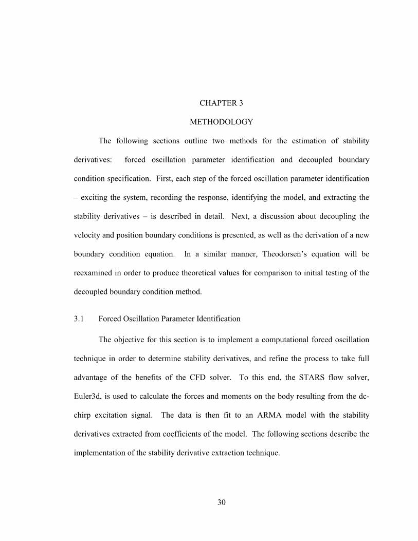
boundary condition equation. In a similar manner, Theodorsens equation will be
reexamined in order to produce theoretical values for comparison to initial testing of the
decoupled boundary condition method.
3.1 Forced Oscillation Parameter Identification
The objective for this section is to implement a computational forced oscillation
technique in order to determine stability derivatives, and refine the process to take full
advantage of the benefits of the CFD solver. To this end, the STARS flow solver,
Euler3d, is used to calculate the forces and moments on the body resulting from the dc-
chirp excitation signal. The data is then fit to an ARMA model with the stability
derivatives extracted from coefficients of the model. The following sections describe the
implementation of the stability derivative extraction technique.

31
3.1.1 CFD Solver
As stated previously, the CFD routine implemented in this research is Euler3d,
which is an Euler flow solver capable of calculating compressible, inviscid flow over a
broad range of Mach numbers from subsonic to supersonic in a non-inertial frame as well
as through transpiration for smaller motions. For a more complete description of the
implementation of STARS and Euler3d, the reader is referred to Gupta [2001] and
Cowan [2003], respectively.
While the flow parameters, such as Mach number, time step, dissipation model,
and solver order, are governed by the control file, the non-inertial motion of the system is
controlled through the dynamic file. Since the zero order, steady state solver was
developed assuming a physically consistent position and velocity relation, this solver
cannot account for non-inertial motion. At the very least, a first-order, time-accurate
solver must be specified in the control file when implementing the non-inertial motion
specification. The first order solver requires more computational time at each time step,
causing the non-inertial formulation to operate more slowly than a method based on a
steady solver. When the use of non-inertial motion is specified in the control file, the
dynamic output file contains the position, velocity, and acceleration of all six degrees of
freedom at every time step.
Information relevant to the current work, contained in the dynamic file, includes
the vector to the origin of rotation, the initial orientation and velocity, if any, and the type
of excitation. The origin of rotation is also the location of the force and moment
calculations in the non-inertial formulation; otherwise, the origin of the grid coordinate
serves as the force and moment reference. For standard aircraft coordinates, a ψ angle of

32
180 degrees is specified because STARS assumes the flow travels in the positive x-
direction. When a non-inertial file is implemented, the flow angles in the control file are
not used by STARS and must be adjusted in the dynamic file. If stability derivative
estimates are desired about an angle of attack or sideslip, then the base angles can be
entered as an initial condition in the dynamic file and the dc-chirp signal can excite the
system around that condition for a given excitation type. For the independent excitation
type, either velocity or position can be held at the initial value while the other is excited.
A different excitation type, the decoupled boundary condition specification, holds the
initial position and velocity constant; even for a non-zero velocity, position is held
constant. The decoupled excitation types require a modification to the acceleration
equation as discussed in Section3.2.2 on page 45.
As previously discussed, transpiration simulates motion by altering the normal
vector of a surface. Flow tangency is then applied to the surface defined by the new
normal vector accurately modeling the actual flow for small changes in the normal
vector. In order to apply transpiration to stability derivative analysis, a vector file
defining the mode shapes in terms of the rigid body degrees of freedom must be
generated about the origin of simulated rotation. The vector file contains the initial
conditions, the excitation type, and the mode shape definition. Again, the excitation
types include: dc-chirp excitation about the initial conditions, independent excitation of
position and velocity, and an inconsistent hold of initial conditions. No modifications to
the equations of the flow solver were required, because transpiration does not assume a
physically consistent boundary condition. In addition, transpiration can be applied with
the zero-order solver, increasing the speed of the stability derivative estimates. When the

33
use of transpiration is specified in the control file, the transpiration output file specifies
the position and velocity of each mode shape at every time step.
3.1.2 Input Excitation
The dc-chirp was selected as the excitation signal based on the low frequency
power content of the signal and the ability to excite high values of velocity and maintain
small displacements. If the rate or velocity terms are not sufficiently excited, the
parameter identification process cannot identify their effects. Should this be the case, the
rate dependent derivatives will be pushed toward zero and the position derivatives altered
to account for the small rate effects.
Since the dominant terms in the forces and moments are typically the angular
displacement and not the angular rates, the damping effects of the rate terms can be
obscured by the displacement terms in the model. In order to produce data that will
facilitate the accurate estimation of the model parameters, the rate terms generally require
greater excitation. The goal is not to make the rate terms dominant, but instead to
increase the effect on the output due to the rate terms to such a degree that the rate
influence is significant when compared to the angular terms. The displacement and
velocity are not excited to the same degree; they are each excited to a degree that
produces comparable output. For example, if an airfoil is pitching about a point n-chord
lengths upstream of the leading edge and the maximum angle of attack to be excited is α,
then pitch rate should be excited to a value that produces an equivalent angle of attack.
( )cnUq ⋅⋅=α
In order to determine the stability derivatives, the signal must excite the terms in
the derivative; namely, angle of attack (α), angle of sideslip (β), roll rate (p), pitch rate

34
(q), and yaw rate (r). However, since the angle of attack is excited with pitch rate, and
sideslip with roll and yaw rates, forcing these terms would be redundant and separating
their effects would difficult at best. If, instead of exciting α and β directly, the plunging
velocity (w) and the side velocity (v) are excited, then α and β are excited through the
plunge and side velocity respectively by the following equations.
= −
uw1sinα
= −
Uv1sinβ
This also allows the effects of q and α& to be separated from each other, as well as β&
from p and r.
As suggested by Iliff [1976] and Klein [1998], each of the five states, v, w, p, q,
and r, can be excited independently. Independently exciting each of the states assists in
the proper identification of the model parameters by allowing the influence of each term
to be determined without the interfering effects of other states. Thus, the identified
model coefficients reflect solely the intended terms and the stability derivatives extracted
from the model parameters do not represent the effects of more than one state. If the
states were excited simultaneously, then the correlations between the states would reduce
the possibility of creating an accurate model and degrade the quality of the stability
derivatives.
Parallel processing is employed in order to reduce the time required to
independently generate the data for the parameter identification of each state. Instead of
sequentially exciting each state, a cluster of computers is used in such a way that each
computer simultaneously runs the flow solver with a different state excited. This
completes the excitation of all the states in the time needed for the excitation of one state.
Additionally, parallel processing eliminates the bias error that can occur in sequential

35
processing. This error can occur when the effects of the previous states excitation have
not dissipated before the next state begins its excitation. The reader is referred to
Boeckmans [2003] work for further information on the use of either clusters or parallel
processing.
With parallel processing, each state receives its own dc-chirp signal, and as such,
each signal must be tailored to the state. In Euler3d, the chirp signal is defined by a non-
dimensional maximum displacement (displ) and sweep frequency (ω). Since the chirp
sweeps frequency, the maximum velocity is then determined by the length of time the
signal is allowed to run. The displacement and velocity equations for the dc-chirp are
repeated below.
( ) ( )[ ]2cos12
tdispltD ⋅−⋅= ω
( ) ( )2sin ttdispltV ⋅⋅⋅⋅= ωω
Selecting the appropriate values for displ and ω is relatively straightforward, but
nonetheless dependent on the time step, the length of signal and the number of points
required for generating the model. The first step is to decide the magnitude of the
displacement, displ, which will provide ample excitation yet remain within the small
disturbance assumptions of the stability derivatives. At higher angles of attack, a smaller
displacement may be required to keep to a locally linear region. In turn, omega is found
by specifying the maximum non-dimensional velocity the system is to achieve in the
above velocity equation, resulting in the following equation for ω, where time is the
number of points (np) multiplied by the non-dimensional time step (∆t).
tnpdisplV
∆⋅⋅= maxω

36
The maximum value of the time step is the function of displ, Vmax, and the
minimum number of points needed at the highest frequency (minpt), as seen below. A
smaller time step might be necessary for the flow solver and should be used in such
cases. If one ARMA model is to be used to describe all five states simultaneously, the
time step for each excitation signal must be the same; different time steps would result in
a difference in the influence of previous terms. For example, with a very small time step
a newly shed vortex will be very close to the trailing edge and have a high influence;
whereas, with a larger time step, the vortex would be farther from the trailing edge and,
therefore, have a smaller influence on the forces.
ptVdispt
minmax ⋅=∆
Typically, the value of minpt is selected based on the number of points required
for a smooth plot of the data points; however, a large value for minpt with the same total
number of points will reduce the frequency content of the excitation signal. The
minimum number of points at the highest frequency must be well above the Nyquist
frequency for the ARMA model to accurately include the effects of previous forces and
motions at that frequency. Figure 3.1, below, demonstrates this with a coarse time step
that is above the Nyquist frequency but is insufficient to represent a continuous function.
The discrete change between two points is too large for the model to accurately represent
the effects of the motion at each point. The model would incorrectly attempt to capture a
non-physical step change in the flow instead of capturing the effects of the wake
produced by the previous point.

37
0.0
0.1
0.2
0.3
0.4
0.5
0.6
0.7
0.8
0.9
1.0
0.0 3.0 6.0 9.0 12.0 15.0
Time
Dis
plac
emen
t
Actual Coarse Figure 3.1: The Effects of a Large Time Step on Excitation Signal
The only remaining unknown in the calculation for ω is the number of points to
be generated, np. The number of points required is solely a function of the model size
and the degree of overdetermination (over). Because the best model size is initially
unknown, np is set such that a large range of models can be examined in order to
determine the best model order. The ARMA model is described by na past outputs, nb
past inputs, and nr states as seen in the equation repeated below.
( )[ ] [ ] ( )[ ] [ ] ( )[ ]∑ ∑=
−
=
−⋅+−⋅=na
n
nb
mmn mtxBntyAty
1
1
0
Since the previous inputs and outputs generated the current wake, the coefficients of
these terms represent the influence of the wake on the current forces. Therefore, as a
general guideline, the number of previous terms included in the model order

38
determination should extend to include the wake. For example, if the wake is assumed
negligible n-chord lengths aft of the vehicle, then the number of previous terms (npt) can
be found by the following equation, where distance is the free stream velocity multiplied
by time.
tUcnnpt∆⋅
⋅=
With a general knowledge of the size of the model, the number of data points
needed for each state can be found by the following equation.
( ) overnanbnrnp ⋅+⋅=
Since the model coefficients are determined in a least squared sense, better results are
obtained with more data. However, the computational run time increases with an
increase in the number of points to be generated. Typically, a value of 5 to 10 for the
overdetermination factor is sufficient. If, in the process of determining the best model
order, more data is needed to make larger models, SVD allows for the partitioning of data
from different computational runs. Another signal, with only as many extra points as
needed, can be generated and combined with the previous data in order to generate larger
models.
3.1.3 Parameter Identification
Once the excitation data has been generated by the solver, the loads and motion
terms are combined and formatted for the SVD routine for parameter identification.
Cowan [1998] discusses the SVD routine and de-trending of the data to remove any
offset, which cannot be represented in the ARMA model. The parameter identification
process consists of gathering the generated data and formatting it for the SVD routine of

39
choice. Therefore, the remaining discussion will focus on determination of the number of
modes to include in the model and selecting the best model size.
While the ARMA model can expand to as many degrees of freedom as are
excited, the time scale of a lateral derivative may not be the same as the longitudinal
term, resulting in a different optimal na-nb model for each direction. Forcing all modes
to fit into a single model can result in a poor model for one mode and a better model for a
more dominant mode. Instead, each degree of freedom should determine its own model
size. This will, of course, increase the workload and complexity by tracking the model
size for each mode, but the independent examination of each mode should provide better
estimates and understanding, which could then be applied to an investigation into
subsequent modes.
In order to conduct a model size sweep, each model in the range of na-nb is
generated and then compared to the data. The best model can be determined based on the
RMS of the error between the model and the data or the RMS of the correlation error;
however, both measures can be misleading. Graphically plotting the data and the ARMA
model predictions is the most reliable way to determine the best model. To plot and
compare each model would be a laborious process, instead, the RMS of both means can
narrow the field of candidate models and provide insight into model convergence. Some
models may oscillate about the data giving a misleadingly small RMS value when in fact
the model does a poor job of predicting the data. Optimally, a new data set would be
generated for the RMS comparison, so that the data used to generate the models is not
also used to determine the quality of the fit. However, the time involved in generating a
new data set limits the application of this principle.

40
3.1.4 Extracting Stability Derivatives
Once the best ARMA model has been identified, extracting the steady and quasi-
steady stability derivatives from the ARMA model consists of applying steady and quasi-
steady conditions for the position and velocity terms and small perturbation theory for the
previous forces terms. This process is best described through a demonstration on a small
ARMA model with na equal to 2, nb equal to 3, and nr equal to 1. The ARMA model
then has the following form:
( ) ( ) ( ) ( ) ( ) ( )2121 21021 −⋅+−⋅+⋅+−⋅+−⋅= tXBtXBtXBtYAtYAtY
For the steady state terms, all the Y and X terms are constant and can be
rearranged to form the following equation, where the derivative of Y with respect to X is
the constant formed by the combination of model coefficients:
( ) ( )tXAABBB
tY ⋅−−++
=21
210
1
This equation can be generalized for any na-nb model size where nr is equal to one.
Therefore, the steady state stability derivative for any model size can be determined by
the equation below:
−= ∑∑=
−
=
na
ii
nb
ii AB
dXdY
1
1
01
If the sum of A term equals unity, the resulting division by zero prevents this method
from working. This condition implies a Markov sequence in which the present terms are
independent of previous terms; however, in a causal relationship, present forces are
dependent on previous states.

41
Quasi-steady stability derivates require further examination as the force and
position terms are no longer constant. Position terms can be determined through a
constant rate equation as follows:
( ) ( ) XtitXitX &⋅∆⋅−=−
Using the above equation, the previous position terms can be found from the current
position and the constant rate, essentially generating the time history of states required to
achieve the current position at a constant rate.
Previous force terms in the ARMA model can be estimated through small
disturbance theory, as demonstrated in the equation below:
( ) ( ) ( ) ( )[ ]itXtXdXdYtYitY −−⋅−=−
Combining the previous position equation and the previous force equation yields the
following equation for the previous forces, where dY/dX is as given above:
( ) ( )dXdYXtitYitY ⋅⋅∆⋅−=− &
By substituting the above expression and the position relation into the general ARMA
model with nr equal to one and simplifying, the following equation is then produced:
( ) ( )
−
⋅+
−
⋅⋅⋅∆⋅−
−⋅=
∑
∑
∑
∑ ∑
∑
∑
=
−
=
=
−
= =
=
−
=na
ii
nb
ii
na
ii
nb
i
na
iii
na
ii
nb
ii
A
iB
A
iABtX
A
BtXtY
1
1
02
1
1
0 1
1
1
0
111&
Therefore, the quasi-steady stability derivative for any na-nb model, where nr is equal to
one, is expressed by the following:

42
−
⋅+
−
⋅⋅⋅∆−=
∑
∑
∑
∑ ∑
=
−
=
=
−
= =na
ii
nb
ii
na
ii
nb
i
na
iii
A
iB
A
iABt
XddY
1
1
02
1
1
0 1
11&
This equation may then be generalized for any order derivative of X as follows, where
X(0) is X, and X(j) is the jth time derivative of X:
−
⋅+
−
⋅⋅⋅∆−=
∑
∑
∑
∑ ∑
=
−
=
=
−
= =na
ii
nb
i
ji
na
ii
nb
i
jna
iiij
j
A
iB
A
iAB
jt
dXdY
1
1
02
1
1
0 1)(
11!
After identifying the parameters of the best-size ARMA model, stability derivative
extraction becomes merely a process of summing coefficients, a process easily performed
in a simple spreadsheet calculation.
3.2 Decoupled Boundary Conditions
The previous sections outlined the current experimental techniques implemented
in a computational framework in which the ARMA model captures the unsteady effects
as well as the effects of position, velocity, and higher order terms. The sole purpose of
the ARMA model is to capture these effects so that each may be accurately separated
from the others. Therefore, if position, velocity, and other terms were excited separately,
the ARMA model would not be required, drastically simplifying the stability derivative
estimation process. The goal, then, becomes to determine a process for decoupling the
position and velocity boundary conditions. This can be accomplished by specifying a
velocity boundary condition and enforcing a constant position or orientation boundary
condition.

43
Figure 3.2, below, demonstrates the separation of the velocity and position
boundary conditions for independent investigation of rate and position. In this case, the
top image represents an airfoil pitching at an angle of attack. The bottom images are the
decoupled components, the left one representing the angle of attack effects, while the
right image represents the velocity profile on the airfoil due to the rotation. The top
figure is equivalent to the sum of the two lower figures.
Figure 3.2: Decoupling Position and Velocity Boundary Conditions
Since the effects of position and velocity may now be calculated separately, the
excitation is also simplified. The rate effects no longer need to be comparable to the
position effects for accurate parameter identification. Furthermore, the frequency content
of the excitation signal is only to ensure the same frequency content in the ARMA model.
If the model is not needed, then neither is the frequency content of the signal. With
displacement held constant for a given rate, the quasi-steady rate effects can be
determined without the displacements reaching the nonlinear range, thereby eliminating
this consideration from the excitation signal. An additional benefit to removing the need
for a model is that the solver does not need to be time accurate. Thus, a faster steady-
state solver can be implemented to determine the quasi-steady forces.

44
Understandably, Euler3d was not designed to implement a steady-state solver in a
non-inertial reference frame; as such, the velocity boundary conditions are instead
applied through transpiration for use with the steady-state solver. In order to remove the
assumptions associated with transpiration to gain a more general solution, the first order
time accurate solver of Euler3d can be used with the non-inertial velocity boundary
condition specification. While slower than the steady-state solver, this is faster than the
second order solver, and since the solution does not need to be time accurate, fewer
iterations are required per time step. The number of time steps is then determined by the
level of convergence of the solution, not the size of the ARMA model. By separating the
excitation of position and velocity, the process of estimating stability derivatives is
dramatically simplified.
3.2.1 Deriving Equations
Because the independent specification of velocity and position is not physically
consistent, the derivation of the boundary condition equations must be revisited.
Consistent boundary conditions are an inherit assumption in the derivation of both the
non-inertial formulation of the boundary conditions in Euler3d and in Theodorsens
results for a pitching and plunging airfoil used later in a validation test case. Neither thin
airfoil theory, which is also use in the validation test case, nor the transpiration boundary
condition equation in Euler3d make the consistency assumption. Understanding the
development of these equations is as important as knowing how to use them.
Since thin airfoil theory does not make the consistent boundary condition
assumption, the development and presentation of the lift and moment equations are left to
Appendix A. Likewise, the transpiration boundary condition equations do not require

45
any modification for a decoupled boundary condition specification, and as such, the
equations are not redeveloped here. Instead, the focus is place on examining the effects
the consistent boundary condition assumption has on both the non-inertial boundary
condition equation in Euler3d and Theodorsens equation.
3.2.2 Non-Inertial Boundary Condition Equation
The development of the non-inertial compressible Euler equations implemented in
STARS is nicely presented in Cowans dissertation [2003]; here the focus is place on the
alterations of these equations to account for the decoupled boundary conditions. The
decoupled boundary condition affects only one equation in Cowans derivation; the
acceleration expressed in the non-inertial frame. Neither the position equation nor the
velocity equation relies on a physically consistent specification of position and velocity;
the user specifies the non-inertial velocities. However, the acceleration equation does
require that the time rate of change of position always equals the velocity. The non-
inertial formulation of the velocity as presented by Cowan is expressed below, where B is
the transformation matrix, Ω is the angular velocity matrix, and r is the radius vector:
xyzt rBVV Ω+= 0
In order to determine the non-inertial acceleration, the derivative of the above
equation proceeds as follows:
xyzxyzxyzt rBrBrBaa && Ω+Ω+Ω+= 20
Normally, the r& term is set equal to the relative velocity Vr; however, with the decoupled
specification, the r& term is zero. Therefore, by changing the transformed acceleration
equation in Euler3d to reflect the non-physical conditions, the non-inertial capabilities of

46
STARS will now properly calculate the forces and moments due to a decoupled rate
specification.
3.2.3 Theodorsens Moment Equation
The following derivation is only used in comparing Theodorsens quasi-steady
results to the stability derivative estimates predicted by Euler3d for the airfoil test case.
Theodorsens moment equation is broken into two components: non-circulatory and
circulatory, the first referring to the bodys motion and the latter to the wake effects.
Each component of the moment equation is examined separately and the results are
combined in the final steps to produce Theodorsens results for an decoupled boundary
condition. The primary reason for the redevelopment of Theodorsens function without
the consistent boundary condition assumption is that the time rate of change of angle of
attack, for instance, is no longer equal to the pitch rate, because α is held constant but the
rate, α& , is specified as non-zero. A review of the geometry of Theodorsens pitching and
plunging thin airfoil is presented in Figure 3.3 below, including the notation used in this
work, which follows Falks derivation [2003]. In this section, b represents the semi-
chord length, a represents the faction of b to the center of rotation, and h is the vertical
displacement with the free stream velocity in the positive X direction. The flow is
assumed inviscid, irrotational, and incompressible.
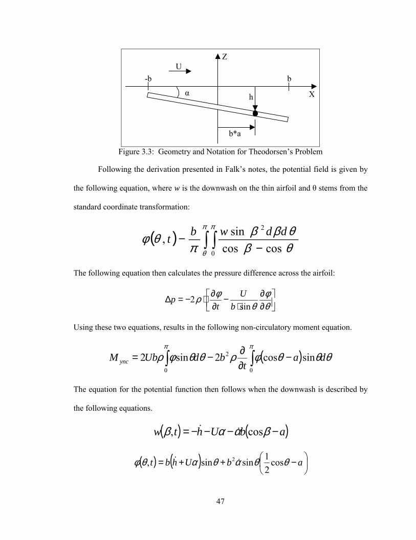
47
Z
X
b-b
h
b*a
U
α
Figure 3.3: Geometry and Notation for Theodorsens Problem
Following the derivation presented in Falks notes, the potential field is given by
the following equation, where w is the downwash on the thin airfoil and θ stems from the
standard coordinate transformation:
( ) ∫ ∫ −−
π
θ
π
θβθββ
πθφ
0
2
coscossin, ddwbt
The following equation then calculates the pressure difference across the airfoil:
∂∂
⋅−
∂∂⋅−=∆
θφ
θφρ
sin2
bU
tp
Using these two equations, results in the following non-circulatory moment equation.
( )∫ ∫ −∂∂−=
π π
θθθφρθθφρ0 0
2 sincos2sin2 dat
bdUbM ync
The equation for the potential function then follows when the downwash is described by
the following equations.
( ) ( )abUhtw −−−−= βααβ cos, &&
( ) ( )
−++= abUhbt θθαθαθφ cos
21sinsin, 2 &&

48
All of the above are the standard equations in the development of Theodorsens
equations; however, with a decoupled boundary condition specification, the final
potential equation is no longer a function of time. Since both position and rate terms are
held constant in time, the derivative of the potential with respect to time is now equal to
zero in the pressure and moment equations. This produces the following equation for the
non-circulator moment:
( )[ ]baUhUbM ync ααρπ && −+= 2
With a consistent boundary condition specification, the derivative of potential with
respect to time yields acceleration terms and the α term becomes anα& term in the second
integral of the moment equation. The α& term in the first integral cancels with the α&
generated by the derivative of potential in the second integral, hence Theodorsens
original equation for the non-circulator moment did not contain the α& term.
For the circulatory portion of the moment equation, the derivation never assumes
that the derivative of α is equal toα& ; instead, the potential function is related to the
vorticity distribution in the wake, which is a function of the downwash on the airfoil.
Therefore, the decoupled boundary condition does not affect the circulatory component
of the moment equation. Setting the reduced frequency, k, equal to zero in the
Theodorsen function is the only requirement to determining the circulatory component of
the quasi-steady moment. With a reduced frequency of zero, Theodorsens function
becomes unity, yielding the following equation for the circulatory quasi-steady moment:
−⋅++⋅= abUhaUbM yc 2
12 2 ααπρ &&

49
Combining the circulatory and non-circulatory components of the pitch moment
equations yields the following equation, after some algebraic simplification:
( ) ( )[ ]ααρπ && baaUhUbM y22 221 −+⋅+⋅=
Note that the moment about the quarter-chord, a = -0.5, does not change with α, in other
words, the aerodynamic center is at the quarter-chord. Also, note that the moment is zero
about the mid-chord, a = 0, if only a pitch rate is applied. This corresponds to data
presented in Theory of Wing Sections for a symmetrically cambered airfoil, which is
equivalent to an airfoil pitched about its mid-chord. For the current work, the stability
derivative, Cmq, is more relevant than the total moment, so the above equation is
reformulated into the following equation, using l/c as the non-dimensional pitch location,
positive aft of the leading edge and negative fore of the leading edge:
2
214
−⋅−=
clCmq π
The above expression from Theodorsens equation, with velocity and position
decoupled, can now be correctly compared to the results obtained by the modified
Euler3d flow solver for a simple airfoil test case. After this, the modified CFD routine
will be used to calculate the stability derivatives of more complex geometries that
Theodorsens cannot predict.

50
CHAPTER 4
4RESULTS AND DISCUSSION
4.1 Forced Oscillation Parameter Identification
The following sections apply the forced oscillation technique in the computational
framework of STARS to two cases and present the results in comparison to theoretical
values. The first test case is presented in conjunction with discussions of grid refinement,
excitation signal parameter selection, model order determination, and interpretation of
results. The following cases will present less on the process and focus instead on the
results of the process. Once the results of the forcing method have been presented, the
decoupled boundary condition specification method will be initially validated with
Theodorsens results. Upon validation of the decoupled method, the first two cases will
be re-evaluated with this new method in order to investigate the relative accuracies of
both processes. Finally, stability derivative estimates for more complex test cases
obtained by the decoupled boundary condition analysis will be presented to demonstrate
the effectiveness of this method.
4.1.1 Horizontal Tail
This single degree of freedom test case is based on an example from Nelsons text
[1998], with some modifications. Instead of a flat plate pivoting 10.998 inches fore of
the leading edge, a NACA 0012 cross-section with a span of 12in and a chord of 2.004in
is used. The airfoil shape removes some of the sharp corners and allows for a smoother
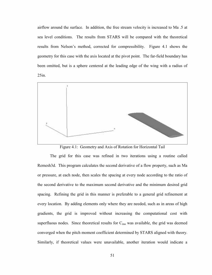
51
airflow around the surface. In addition, the free stream velocity is increased to Ma .5 at
sea level conditions. The results from STARS will be compared with the theoretical
results from Nelsons method, corrected for compressibility. Figure 4.1 shows the
geometry for this case with the axis located at the pivot point. The far-field boundary has
been omitted, but is a sphere centered at the leading edge of the wing with a radius of
25in.
Figure 4.1: Geometry and Axis of Rotation for Horizontal Tail
The grid for this case was refined in two iterations using a routine called
Remesh3d. This program calculates the second derivative of a flow property, such as Ma
or pressure, at each node, then scales the spacing at every node according to the ratio of
the second derivative to the maximum second derivative and the minimum desired grid
spacing. Refining the grid in this manner is preferable to a general grid refinement at
every location. By adding elements only where they are needed, such as in areas of high
gradients, the grid is improved without increasing the computational cost with
superfluous nodes. Since theoretical results for Cmα was available, the grid was deemed
converged when the pitch moment coefficient determined by STARS aligned with theory.
Similarly, if theoretical values were unavailable, another iteration would indicate a
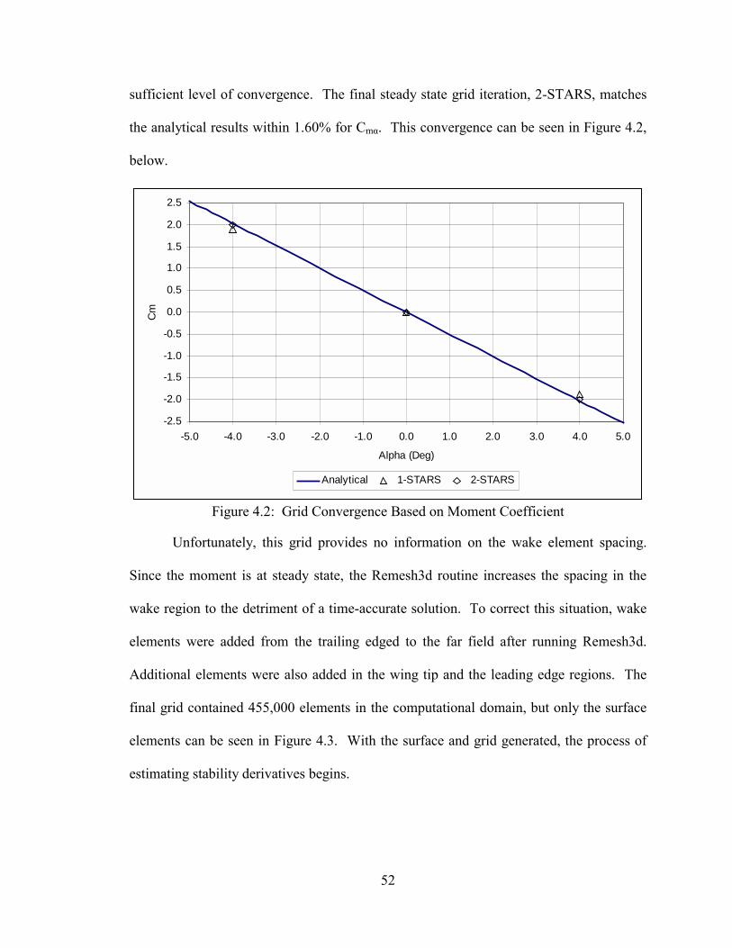
52
sufficient level of convergence. The final steady state grid iteration, 2-STARS, matches
the analytical results within 1.60% for Cmα. This convergence can be seen in Figure 4.2,
below.
-2.5
-2.0
-1.5
-1.0
-0.5
0.0
0.5
1.0
1.5
2.0
2.5
-5.0 -4.0 -3.0 -2.0 -1.0 0.0 1.0 2.0 3.0 4.0 5.0
Alpha (Deg)
Cm
Analytical 1-STARS 2-STARS
Figure 4.2: Grid Convergence Based on Moment Coefficient
Unfortunately, this grid provides no information on the wake element spacing.
Since the moment is at steady state, the Remesh3d routine increases the spacing in the
wake region to the detriment of a time-accurate solution. To correct this situation, wake
elements were added from the trailing edged to the far field after running Remesh3d.
Additional elements were also added in the wing tip and the leading edge regions. The
final grid contained 455,000 elements in the computational domain, but only the surface
elements can be seen in Figure 4.3. With the surface and grid generated, the process of
estimating stability derivatives begins.

53
Figure 4.3: Close-up of Surface Grid for Horizontal Tail
Following the procedure outlined in the Methodology Section, the first step in
estimating stability derivatives is to determine the parameters of the excitation signal.
For this test case, the motion is constrained to pitch only about the y-axis in Figure 4.1; as
such, the excitation signal excites pitch angle and pitch rate. In order to stay within the
linear lift region and avoid stall, the maximum angle of attack is set to 4deg. The pitch
rate required to yield a comparable effect in the pitch moment is given by the following
equation for small angles and large l, the distance from quarter-chord to center of
rotation.
Ulq ⋅=α
Given the geometry and free stream velocity for this case, the maximum pitch rate
should be 2232deg/sec. After plotting the dc-chirp signal with these parameters and the

54
time step as a function of the minimum number of points at the highest frequency, the
best value of minpt was determined to be 35. Higher numbers reduced the frequency
content without adding significant definition to the signal, while lower numbers produced
a sampling rate that was too small at the highest frequency.
The maximum time step can now be calculated as 5.12e-5sec, which is rounded
down to 5.0e-5sec. With the time step now determined, the number of data points
required for parameter identification can be found. If the wakes effect becomes
negligible 8-chords aft of the trailing edge, then 50 time steps are required to reach this
point. The overdetermination of the mathematical model depends on the size of the
model; however, if over is specified to be 8, then the largest model has an
overdetermination factor of 8 and the smaller models will have a larger
overdetermination factor. This yields a requirement of 800 points for the parameter
identification. With this, all the terms of the excitation signal can be calculated in their
dimensionless form. The displ term is the maximum angle of attack in radians, while
Vmax in the ω equation is given by the following equation, where q is the maximum pitch
rate in rad/sec and refdim is specified in the control file, typically as 1:
UrefqV dim
max⋅=
This combination of parameters results in the excitation of the angle of attack and
the pitch rate seen in Figure 4.4, below. While the pitch rate, q, may seem too large, this
value is necessary in order for the parameter identification routine to properly identify the
effects of both position and velocity. Smaller values of q will corrupt the estimation of
its effects on the moment, essentially drowning the effect of pitch rate in the effect of
pitch angle. However, an extremely large pitch rate could excite terms that would not

55
appear under normal operating conditions, and could produce effects that could not be
correctly eliminated through the ARMA model, such a shock waves due to motion not
flight condition.
-3.0E+03
-2.0E+03
-1.0E+03
0.0E+00
1.0E+03
2.0E+03
3.0E+03
0.0E+00 1.0E-02 2.0E-02 3.0E-02 4.0E-02Time (sec)
Pitc
h R
ate
(deg
/sec
)
-4.5E+00
-3.0E+00
-1.5E+00
0.0E+00
1.5E+00
3.0E+00
4.5E+00
Alpha (deg)
Pitch Rate Alpha
Figure 4.4: Pitch Rate and Angle of Attack (Alpha) for DC-Chirp
Figure 4.5 presents the control file implemented with the horizontal tail test case.
STARS ran for 24.56 hours to generate the 800 data points, with 50 iterations per time
step to insure convergence at each time step. By combining the load and dynamics files,
as discussed in the Methodology Section, the data can be compiled into the proper form
for the SVD routine.

56
&control dt = 0.3348d0, mach = 0.50d0, gamma = 1.40d0, alpha = 0.0d0, diss = 1.00d0, beta = 0.0d0, cfl = 0.5d0, refdim = 1.0d0,
nstp = 800, istrt = .true., nout = 800, iaero = .true., ncyc = 50, idynm = .true., isol = 2, ielast = .false., idiss = 1, ifree = .true., ipnt = 1, iforce = .false.,
omega = 3.5057d-4, nr = 1, ratio = 700 ainf = 1.3392d4, displ = 6.981317d-2, rhoinf = 1.146d-7,
Figure 4.5: Control File Parameters for Horizontal Tail
After generating a range of models for na, 1 to 50, and nb, 3 to 50, each model
was given inputs from the excitation signal; and, the error between the model and the
STARS data was tabulated. The best na-nb model according to the RMS error between
the signal and data was a 29-49, whereas the 35-14 model had the lowest RMS of the
cross correlation. Since the ARMA model can oscillate about the actual STARS output
and produce a small RMS, the only true way to determine the quality of the model is to
plot the models output with the STARS data. The pitch moment coefficient time
histories of the two ARMA models are extremely similar; both models match the STARS
output quite well, as seen in Figure 4.6. Although the ARMA line is based on the 35-14
model, the graph can represent both the 29-49 model and the 35-14 model, since the
differences are essentially imperceptible.

57
-6.00
-4.00
-2.00
0.00
2.00
4.00
0.00 0.01 0.02 0.03 0.04
Time (sec)
Cm
ARMA STARS
Figure 4.6: Comparison of Cm for ARMA Model and STARS
Through the process outlined in the Methodology Section, the stability derivative
can be extracted from the ARMA model coefficients. Figure 4.7 below contains the
spreadsheet data used to extract the stability derivatives for the 35-14 ARMA model.
The As are the previous force coefficients, the Bs are the current and previous position
coefficients, and the inputs are the dimensionless time step and the theoretical values for
percent difference calculations.

58
dt* 0.3348 Cmalpha CmqCmalpha -2.9100E+01 -2.852E+01 -3.484E+02
Cmq -3.4850E+02 -1.9780% -0.0162%
Sum(B's) Sum(A*j) Sum(B*(j-1)) 1-Sum(A's) (1-Sum(A's))^2-3.92085E-01 5.32995E-03 2.16612E+01 2.85229E-04 8.13555E-08
OutputInput
A's B's j A*j B*(j-1)
3.9158582E+00 2.1270306E+04 1 3.9158582E+00 0.0000000E+00-6.0783746E+00 -4.3510418E+04 2 -1.2156749E+01 -4.3510418E+044.5180339E+00 1.4716748E+04 3 1.3554102E+01 2.9433496E+04
-1.2235178E+00 -1.2182433E+03 4 -4.8940712E+00 -3.6547300E+03-4.4795634E-01 -8.2015002E+03 5 -2.2397817E+00 -3.2806001E+042.5505407E-01 3.9455524E+04 6 1.5303244E+00 1.9727762E+053.1928360E-01 -5.0838306E+03 7 2.2349852E+00 -3.0502984E+04
-3.5412394E-01 2.1656047E+04 8 -2.8329915E+00 1.5159233E+05-1.0718900E-01 -5.0834416E+04 9 -9.6470102E-01 -4.0667533E+054.3597790E-01 -1.7815644E+04 10 4.3597790E+00 -1.6034079E+05
-1.2707976E-01 1.9454999E+04 11 -1.3978774E+00 1.9454999E+05-5.5909591E-01 -1.3731269E+04 12 -6.7091509E+00 -1.5104396E+058.9276947E-01 5.4234526E+04 13 1.1606003E+01 6.5081431E+05
-6.2806095E-01 -3.0393220E+04 14 -8.7928534E+00 -3.9511186E+052.7803843E-01 15 4.1705765E+00 0.0000000E+00
-1.9799604E-01 16 -3.1679367E+00 0.0000000E+001.2045208E-01 17 2.0476853E+00 0.0000000E+00
-3.1384154E-02 18 -5.6491478E-01 0.0000000E+001.8937286E-01 19 3.5980844E+00 0.0000000E+00
-2.2424657E-01 20 -4.4849314E+00 0.0000000E+00-3.0910703E-01 21 -6.4912476E+00 0.0000000E+008.0676274E-01 22 1.7748780E+01 0.0000000E+00
-5.3162020E-01 23 -1.2227265E+01 0.0000000E+001.1126588E-01 24 2.6703811E+00 0.0000000E+00
-2.2569922E-01 25 -5.6424805E+00 0.0000000E+004.1113520E-01 26 1.0689515E+01 0.0000000E+00
-4.2391787E-01 27 -1.1445782E+01 0.0000000E+002.0448730E-01 28 5.7256443E+00 0.0000000E+004.0537209E-01 29 1.1755791E+01 0.0000000E+00
-7.0657333E-01 30 -2.1197200E+01 0.0000000E+003.8411769E-01 31 1.1907648E+01 0.0000000E+001.3207324E-02 32 4.2263436E-01 0.0000000E+00
-3.1828114E-01 33 -1.0503278E+01 0.0000000E+003.6549423E-01 34 1.2426804E+01 0.0000000E+00
-1.3274440E-01 35 -4.6460542E+00 0.0000000E+00
Figure 4.7: Extraction of Stability Derivatives from the 35-14 ARMA Model
The extracted stability derivatives are very close to the theoretical values for the
35-14 ARMA model. The stability derivative extracted from the 29-49 model should be
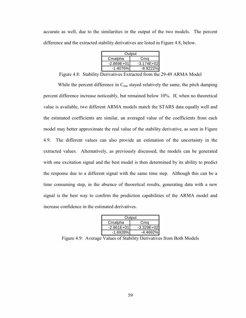
59
accurate as well, due to the similarities in the output of the two models. The percent
difference and the extracted stability derivatives are listed in Figure 4.8, below.
Cmalpha Cmq-2.869E+01 -3.174E+02
-1.4076% -8.9222%
Output
Figure 4.8: Stability Derivatives Extracted from the 29-49 ARMA Model
While the percent difference in Cmα stayed relatively the same, the pitch damping
percent difference increase noticeably, but remained below 10%. If, when no theoretical
value is available, two different ARMA models match the STARS data equally well and
the estimated coefficients are similar, an averaged value of the coefficients from each
model may better approximate the real value of the stability derivative, as seen in Figure
4.9. The different values can also provide an estimation of the uncertainty in the
extracted values. Alternatively, as previously discussed, the models can be generated
with one excitation signal and the best model is then determined by its ability to predict
the response due to a different signal with the same time step. Although this can be a
time consuming step, in the absence of theoretical results, generating data with a new
signal is the best way to confirm the prediction capabilities of the ARMA model and
increase confidence in the estimated derivatives.
Cmalpha Cmq-2.861E+01 -3.329E+02
-1.6928% -4.4692%
Output
Figure 4.9: Average Values of Stability Derivatives from Both Models

60
Given that the theoretical values are available, the analytical quasi-steady pitch
moment time history can be created and compared with the quasi-steady values predicted
by the ARMA model. Figure 4.10 reveals how accurately the 35-14 ARMA model
matches the analytical response. This may initially appear to be a redundant figure in that
the ARMA model agrees with the STARS data; however, the data used to generate the
model is much different than the quasi-steady response predicted by the analytical results.
-3.500
-3.000
-2.500
-2.000
-1.500
-1.000
-0.500
0.000
0.500
1.000
1.500
0.000 0.005 0.010 0.015 0.020 0.025 0.030 0.035 0.040
Time (sec)
Cm
Analytical ss ARMA
Figure 4.10: Comparison of Cm for Analytical and Quasi-Steady ARMA
Since large excitations violate the assumptions of stability derivative analysis, the
ARMA model is used to transition from the unsteady data to the quasi-steady stability
derivatives. After the ARMA model is fit to the fully unsteady data produced by STARS,
the ARMA model is given quasi-steady conditions to remove the unsteady terms and
extract the quasi-steady stability derivatives. The purpose of the ARMA model is to
correctly account for the unsteadiness produced during excitation in order to properly
eliminate it from the stability derivative calculations. Figure 4.11 demonstrates the

61
unsteady filtering that the ARMA model provides. The difference, both in phase and
amplitude, between the analytical and the STARS data results from unsteady and higher
order terms not included in the analytical model; however, the ARMA model can be used
to translate the unsteady STARS data into the quasi-steady analytical results. The
unsteady terms are neither Gaussian nor white as is assumed during the filtering of
experimental data. Also, the large magnitude of the unsteady effects is due to the
extremely large rate excitation required for the proper identification of the rate effects.
Essentially, in order to accurately estimate the quasi-steady rate term, the unsteady terms
must also be excited. The Analytical line is covered by the ss ARMA points;
similarly, the STARS points obscure the ARMA line.
-6.00
-5.00
-4.00
-3.00
-2.00
-1.00
0.00
1.00
2.00
3.00
4.00
0.00 0.01 0.02 0.03 0.04
Time (sec)
Cm
ARMA STARS Analytical ss ARMA
Figure 4.11: Comparison of Unsteady STARS to Quasi-Steady Analytical Results

62
4.1.2 Dihedral Wing
The next case to be examined is a dihedral wing, allowing for both longitudinal
and lateral stability derivative analysis. Figure 4.12 presents the geometry of this test
case with a chord of 2 inches, a span of 8 inches, a NACA 0009 cross-section, and 5
degrees of dihedral. The axis is on the origin of rotation, which is located at the
centerline leading edge, 0.5 inches above the plane of the root chord. Flight conditions
are specified as standard sea level at Mach 0.4. Wake elements are included in the
ellipsoidal computational domain in order to capture the transients in the flow field that
result from the excitation of the wing.
Figure 4.12: Geometry of Dihedral Wing

63
A grid resolution study was conducted, as before, implementing the Remesh3d
procedure; however, with this case, the effects of sideslip angle, β, had to be examined as
well. For angle of attack, the steady state solution was determined at -5, 0, and 5 degrees
α for each grid refinement iteration. The results of this grid convergence can be seen in
Figure 4.13, below. From this figure, the initial grid would have been sufficient to
capture longitudinal effects, but grid refinement for the lateral direction can affect the
longitudinal results, although it does not in this case. Therefore, the pitch moment plot
was created to ensure that the lateral refinement did not adversely affect the longitudinal
results. Roll angle was not investigated since, at zero α, all roll angles are equivalent.
-0.15
-0.10
-0.05
0.00
0.05
0.10
0.15
-6.0 -5.0 -4.0 -3.0 -2.0 -1.0 0.0 1.0 2.0 3.0 4.0 5.0 6.0
Alpha (Deg)
Cm
Datcom 1-STARS 2-STARS 3-STARS
Figure 4.13: Longitudinal Grid Convergence

64
As stated above, grid convergence based on lateral effects was also investigated.
At zero degrees angle of attack, the system was given -5, 0, and 5 degrees β in order to
determine the capability of the grid to accurately capture sideslip. Using the Remesh3d
program to again generate more elements in areas of high gradients, the grid was
converged as seen in Figure 4.14 below according to the roll moment induced by the
sideslip angle. While the values do not lie directly on the analytical line obtained from
the Datcom equations, the grid was refined until the results were independent. The
Datcom method is somewhat empirical, and the effect of roll moment due to sideslip is
small. For this geometry, both of these factors contribute to the less than perfect
alignment between the converged grid and the analytical line. In the absence of
analytical results, Figure 4.14 indicates a converged grid, which should be sufficient for a
method independent of previous estimates.
-6.0E-03
-4.0E-03
-2.0E-03
0.0E+00
2.0E-03
4.0E-03
6.0E-03
-6.0 -5.0 -4.0 -3.0 -2.0 -1.0 0.0 1.0 2.0 3.0 4.0 5.0 6.0
beta (Deg)
Cl
Datcom 1-STARS 2-STARS 3-STARS
Figure 4.14: Lateral Grid Convergence

65
By following the same procedure as before, the control parameters for pitch
excitation seen in Figure 4.15 are produced. The excitation parameters translate to a
maximum angle of attack of 6 degrees and a maximum pitch rate of 32,250 degrees per
second. This is an extremely large value of q; however, it is the amount of q needed for
the proper identification of pitch damping. This value for q generates an equivalent angle
of attack of 3 degrees at the quarter-chord and 6 degrees at the half-chord. With a
comparable angle, the large rate has a comparable effect, which can be identified by the
ARMA model. Such a large value also indicates that the effect of Cmq will be small;
however, it is still the dominant pitch damping term [Datcom 1978] and, therefore,
requires accurate estimation.
&controldt = 8.0352d-2, mach = 0.40d,gamma = 1.40d0, alpha = 0.0d0,diss = 1.00d0, beta = 0.0d0,cfl = 0.5d0, refdim = 1.0d0,
nstp = 4000, istrt = .true.,nout = 4000, iaero = .false.,ncyc = 75, idynm = .true.,isol = 2, ielast = .false.,idiss = 1, ifree = .true.,ipnt = 1, iforce = .false.,
ratio = 800d0 nr = 1,omega = 3.2019d-3 ainf = 1.3392d4,displ = 1.0472d-1 rhoinf = 1.146d-7,
Figure 4.15: Control File for Pitch Excitation
With such a small time step, the ARMA model would need about 250 terms in
order to account for wake effects 10 chord lengths downstream. Determining the model
parameters for a model of this size would be a rather large and time consuming
undertaking; instead, the data was re-sampled. By taking every fifth point, the time step
for the ARMA model, not the flow solver, increases by a factor of five and the number of

66
terms in the ARMA model reduces by a factor of five. An ARMA model of 50 terms is
much easier to identify. While the flow solver requires a smaller time step in order to
ensure convergence at each step, the ARMA model time step can be larger, so long as it
stays sufficiently above the Nyquist frequency.
The same process was repeated for sideslip and for roll rate effects, but not for
roll angle. Likewise, a plunging velocity and a side velocity were also excited in order to
separate the effects of α& from pitch rate and β& effects from yaw rate as discussed in the
Methodology Section. However, the failure of this method to accurately predict the
longitudinal effects precludes any discussion of the lateral direction and velocity
excitations.
Exciting the pitching motion according to the parameters listed in Figure 4.15 and
re-sampling the data, as discussed above, produces the pitch moment coefficient time
history response seen in Figure 4.16. This figure is very different from the plot presented
for the horizontal tail because the unsteady effects are magnified tenfold for this case.
Since the excitation is a factor of ten larger, the unsteady effects are equivalent in
magnitude as the steady and quasi-steady stability derivatives, causing a great deal of
both constructive and destructive effects. Also included in the figure is a line
representing the ARMA model which best fit the data according to the RMS of the
correlation error. While this model does an extremely poor job of matching the STARS
data, the 7-5 model did better than any of the other models examined in the na 1 to 40, nb
2-50 sweep. Due to the poor performance of the 7-5 ARMA model to predict the data
used to train the model, there is little hope of achieving accurate stability derivatives.

67
-5.E-01
-4.E-01
-3.E-01
-2.E-01
-1.E-01
0.E+00
1.E-01
2.E-01
3.E-01
4.E-01
5.E-01
0.E+00 1.E-02 2.E-02 3.E-02 4.E-02 5.E-02 6.E-02
Time (sec)
Cm
ARMA STARS
Figure 4.16: Resampled Pitch Moment Coefficient Time History with ARMA Model
As expected, the error in the stability derivatives is high. For Cmα, the percent
difference between the thin airfoil theory estimate, corrected for compressibility and
aspect ratio, and the STARS prediction is almost 40%; the percent difference of Cmq is a
staggering 140%. Figure 4.17 attempts to compare the analytical response predicted by
thin airfoil theory and small disturbance theory to the response obtained through the
ARMA model coefficients. The large error in Cmq can be seen by the large difference on
the right side of the figure where q is largest and the response predicted by the stability
derivatives extracted from the ARMA model extend off the chart.

68
-5.E-01
-4.E-01
-3.E-01
-2.E-01
-1.E-01
0.E+00
1.E-01
2.E-01
3.E-01
4.E-01
5.E-01
0.E+00 1.E-02 2.E-02 3.E-02 4.E-02 5.E-02 6.E-02
Time (sec)
Cm
Analytical ss ARMA
Figure 4.17: Comparison of Cm for Analytical and Quasi-Steady ARMA
Although the forced oscillation parameter identification method failed for this
case, it was highly accurate in predicting the stability derivatives for the horizontal tail.
This method cannot identify small magnitude terms well without extreme excitation,
which leads to a very small time step and increased unsteadiness. For the identification
of dominant terms, this parameter identification routine works quite well. Another
drawback to this method is the large amount of time required to generate a time accurate
solution over enough time steps to generate identification data. The process of selecting
the best model is also an issue of concern. Without theoretical values or estimates, the
surest way to determine the best model is to run yet another time accurate solution so that
the models can predict data not used in the training process. This method could be
69
helpful in analyzing existing data or in determining the dominant terms affecting the
forces on a system. In this implementation, less dominate terms would not be
intentionally over excited in order to produce forces comparable to the dominate terms.
To achieve the objectives of this work, a more robust and accurate technique was sought
to estimate stability derivatives in a timelier manner.
4.2 Decoupled Boundary Condition Specification
The following sections present the estimates of stability derivatives by applying
the velocity boundary condition separately from the position boundary condition in
STARS. This is accomplished through both modified non-inertial rate specification and
transpiration. While transpiration adds some limiting assumptions, the time saved for the
more complicated test cases is worth the slight loss of accuracy and amplitude
limitations. Unlike the previous method, no extreme excitation signal is required to
identify the individual effects; they are excited independently. Since the decoupled
boundary condition method is based on quasi-steady forces and moments, no model is
required to make the results fit the stability derivative assumptions. As this method
greatly simplifies the process of estimating stability derivatives, the results of the
following sections focus on comparison with the previous method, as well as with
analytical, empirical, and flight-test data for a variety of geometries over a broad range of
Mach numbers.

70
4.2.1 Airfoil
In order to investigate the accuracy of estimating stability derivatives by the
separate excitation of velocity and position, a simple, well-developed test case was
examined. For this initial case, an NACA 0012 airfoil with a unit chord is first pitched
about the leading edge, then about various points fore and aft of the leading edge to
estimate Cmq. Grid convergence for this test case is not investigated, as this grid has
shown itself to be sufficient and well converged in previous works [ONeill 2003]. The
infinite span airfoil is simulated by a symmetry plane on one side of the 0.2inch wide
computational domain and a wall boundary on the other side. Inviscid, Euler solvers treat
a wall boundary the same as a symmetry plane, since there is not a no-slip condition on
the wall boundary. Figure 4.18 presents the geometry for this airfoil test case.
Figure 4.18: Geometry for Airfoil Test Case

71
The flight condition for this case is standard sea-level conditions at Ma 0.3. The
Mach number is intentionally set to a low value for a better comparison of pitch moment
results with incompressible theory. If the non-inertial formulation is used with the
modifications discussed in the Methodology Section, then the dynamic file is given the
origin of the non-inertial frame and the constant pitch rate while holding α constant at
zero. If transpiration is used to simulate the motion, then the vector file is generated to
model the rigid body pitch motion about the center of rotation. Again, a constant pitch
rate is specified in the vector file while holding α at zero. In order to estimate the
derivative with respect to pitch rate through finite difference approximation, at least two
data points are required, each one at a different value of q; more points are necessary to
demonstrate that the stability derivative lies in the linear range.
Initially, Cmq about the leading edge is estimated by both the non-inertial and
transpiration methods and compared to the analytical results predicted by thin airfoil
theory, corrected for compressibility by the Prandtl-Glauert correction. A broad range of
instantaneous pitch rates is applied to the airfoil through both means in order to determine
the quasi-steady moment due to each rate. Stability derivatives are then estimated by
finite difference equations between points. The results are presented in Figure 4.19,
below, with both the theoretical line of Cm versus q and the non-inertial data points, as
well as the transpiration data points. Although the STARS predictions are slightly higher
than the theoretical values, the linear trend throughout the range of pitch rates is
demonstrated for both the non-inertial and transpiration data points. The non-inertial data
set is closer to the thin airfoil theory in both value and slope than the transpiration data
set.

72
-4.00E-03
-3.50E-03
-3.00E-03
-2.50E-03
-2.00E-03
-1.50E-03
-1.00E-03
-5.00E-04
0.00E+00
5.00E-04
0 50 100 150 200 250 300 350 400 450 500
Pitch Rate (Deg/sec)
Cm
Non-Inertial Transpiration Thin Airfoil Theory
Figure 4.19: Pitch Moment Coefficient Due to Pitch Rate Only
From the above figure, the analytical and STARS predicted values for Cmq can be
determined. The values for Cmq for all cases along with their percent difference from the
analytical value obtained from thin airfoil theory are presented in Figure 4.20. From the
figure, the percent difference more than doubles when using transpiration as opposed to
the non-inertial rate specification; however, the percent difference is still sufficient for
preliminary estimates.
Analytical Non-Inertial TranspirationCmq -3.293 -3.174 -3.005
% Diff - -3.635% -8.759% Figure 4.20: Comparison of Pitch Damping Results for Airfoil Test Case
To further explore this test case, Cmq was estimated for varying pitch locations.
At each location, Cmq is determined through the finite difference approximation between
a pitch rate of 0 and 20 deg/sec. These computational experiments were conducted using
both the non-inertial and transpiration formulations. Because the forces do not change
with pitch location for the zero pitch rate case, the same data can be use at each location

73
if the forces are properly shifted in order to determine the pitch moment for each pitching
location at zero q. At each location, the dynamic file is given the appropriate non-inertial
origin or a new vector file is generated with the origin of rotation properly indicated.
Figure 4.21 presents the results of this examination for various l/c locations, where l is
the distance from the center of rotation to the leading edge, positive for rotating aft of the
leading edge. The values predicted by Theodorsen lie directly on top of those predicted
by thin airfoil theory. The Datcom method and the method presented in Nelsons text are
very similar, differing only slightly as the origin of rotation is moved further from the
airfoil. The STARS non-inertial and transpiration data also seem very similar to each
other and accurate to the analytical values.
-1800
-1600
-1400
-1200
-1000
-800
-600
-400
-200
0
-11.00 -9.00 -7.00 -5.00 -3.00 -1.00 1.00 3.00 5.00 7.00 9.00 11.00
l/c (+aft, - fore of LE)
Cm
q
TAFT Theodorsen DatcomNelson Transpiration Non-Inertial
Figure 4.21: Pitch Damping Coefficient Versus Pitch Location

74
Figure 4.22, below is the same graph as in Figure 4.21, but focused on a smaller
range with the addition of 10% error bars to examine the results more closely. The non-
inertial and transpiration data still match the thin airfoil theory and Theodorsen lines, but
the differences between these and the Datcom and Nelsons method are highlighted.
Both the Datcom method and Nelsons method are based on the assumption that the lift
produced acts at the quarter chord, which is correct when pitching about a point away
from the airfoil. However, when pitching about a point near or on the airfoil the center of
pressure is no longer at the quarter chord, making the assumptions of the two methods
invalid. STARS transpiration and non-inertial rate specifications are accurate even in this
region, with the non-inertial data more closely approximating the theoretical values.
-40
-35
-30
-25
-20
-15
-10
-5
0
-1.25 -1.00 -0.75 -0.50 -0.25 0.00 0.25 0.50 0.75 1.00 1.25 1.50 1.75 2.00 2.25
l/c (+aft, - fore of LE)
Cm
q
TAFT Theodorsen DatcomNelson Transpiration Non-Inertial
Figure 4.22: A Closer Look at Pitch Damping Coefficient Versus Pitch Location

75
This simple test case demonstrates the viability of separating the effects of
velocity from position. Due to this separation, the conning or oscillatory motion
implemented in other methods [Park 1999] is not required to ensure that the angles
remain in the linear range. In addition, the method is completely general, in that a model
is not needed and a model form does not have to be assumed; no geometry or flow
restrictions are required due to model form or assumptions. Even coupling between the
longitudinal and lateral directions is permissible, which would severely hinder the
accurate estimate of stability derivatives by any method employing the decoupled
equations of motion, such as the maximum likelihood estimator. Iliff [1976] states that
flight experiments that failed to be properly identified by the maximum likelihood
estimator contained coupling of the longitudinal and lateral directions or locally transonic
flows, neither of which should cause failure of the decoupled boundary condition method.
In the following sections, the first two cases presented will be reexamined with
this new method and compared to both previous results and analytical predictions.
Following that presentation, a slightly more complicated three-dimensional case will be
examined and compared to the Datcom methods. Then finally, a full aircraft, the F-18A,
will be evaluated with this new method and compared to flight test data in the transonic
regime.

76
4.2.2 Horizontal Tail
Since the separation of velocity from position has shown itself to be a viable
method for determining stability derivatives, this process will be applied to the forced
oscillation test cases. Although not required, this case will use an excitation signal and
the ARMA model as before, but only in order to better compare with the results of the
previous method. The first case examined was the horizontal tail pitching about a point
10.998 inches fore of the leading edge. Figure 4.1 depicted the geometry of this test case,
and is repeated below. For this test case, the stability derivatives will be estimated by the
same process as before with the exception that the pitch rate will be excited
independently of the pitch angle. This is accomplished through the modified boundary
condition equation discussed in the Methodology Section.
Figure 4.1: Geometry and Axis of Rotation for Horizontal Tail
For an accurate comparison with the previous results of this test case, the exact
same excitation signal is used; the velocity excitation signal is applied during one
computational run and the position excitation during a separate run. The moments
produced by the separate excitations are then summed to generate the total moment due
to position and velocity at any given instant of the excitation signal. Figure 4.23 below

77
shows the angle and rate components of the pitch moment coefficient as well as the
summed coefficient. The phase and amplitude effects of each component are reflected in
the line representing the combination of the two component signals.
-3.5E+00
-2.5E+00
-1.5E+00
-5.0E-01
5.0E-01
1.5E+00
2.5E+00
0.0E+00 1.0E-02 2.0E-02 3.0E-02 4.0E-02
Time (sec)
Cm
Alpha q Sum
Figure 4.23: Pitch Moment Coefficient from Separate Excitation
Using the summed pitch moment coefficient time history for the parameter
identification as before, the ARMA model that best represents the data is the 23-21
model. This ARMA model had the minimum RMS of the cross-correlation. Model order
was determined by the same model sweep as before, na 1 to 50 and nb 3 to 50. A
comparison of the ARMA model and the STARS data can be seen in Figure 4.24. The
23-21 model does an excellent job of fitting the data over the entire range, indicating that
the stability derivative extracted from the ARMA model will be accurate as well.

78
-3.5E+00
-2.5E+00
-1.5E+00
-5.0E-01
5.0E-01
1.5E+00
0.0E+00 1.0E-02 2.0E-02 3.0E-02 4.0E-02
Time (sec)
Cm
Sum ARMA
Figure 4.24: Comparison of STARS Data and ARMA Model
From the model coefficients and the previously discussed spreadsheet, Figure 4.7,
values for the stability derivatives were determined and presented in Figure 4.25. The 3-
10 model had the minimum RMS of the error, but was noticeably different from the 23-
21 model and did not match the data as well in regions of large pitch rate; however, the
error in the stability derivatives estimate from that model was only slightly higher than
the 23-21 model. The percent difference of the stability derivative obtained through the
separate excitation of angle and rate is comparable to the averaged values obtained by the
simultaneous excitation.
Cmalpha Cmq-28.70179 -334.478-1.3669% -4.0228%
Figure 4.25: Stability Derivatives Extracted from 23-21 ARMA Model

79
While the best model for the simultaneous excitation was a 35-14 model, the 23-
21 model was best for the independent excitation; yet, both models produced comparable
results. Figure 4.26 demonstrates the reason for the difference in the models. This figure
contains the forced oscillation data as well as the summed data from the separate
excitation. The required models are different because the data sets contain differing
amounts of unsteadiness. For the simultaneous case, more unsteady terms are excited
resulting in a higher order model to remove the unsteady effects in order to determine the
quasi-steady stability derivatives. By exciting the terms independently, the summed data
contains less unsteadiness; however, the ARMA model still properly models the terms
that are present, demonstrating the flexibility of the ARMA model in capturing the
relevant flow physics.
-6.0E+00
-4.0E+00
-2.0E+00
0.0E+00
2.0E+00
4.0E+00
0.0E+00 1.0E-02 2.0E-02 3.0E-02 4.0E-02
Time (sec)
Cm
Simultaneous Separate
Figure 4.26: Pitch Moment Comparison of Simultaneous and Separate Excitation

80
Another interesting comparison is found in Figure 4.27, below, this figure plots
the total pitch moment coefficient from the separate excitation to the analytical response
for the same excitation. The small percent difference in the rate stability derivative
becomes perceptible only at the largest values for pitch rate. For all reasonable values of
pitch rate, the difference is unnoticeable. Since the separate excitation can accurately
match the analytical response with out extracting the stability derivatives from the
ARMA model, the excitation signal and ARMA model may not even be needed.
-3.5E+00
-3.0E+00
-2.5E+00
-2.0E+00
-1.5E+00
-1.0E+00
-5.0E-01
0.0E+00
5.0E-01
1.0E+00
1.5E+00
0.0E+00 5.0E-03 1.0E-02 1.5E-02 2.0E-02 2.5E-02 3.0E-02 3.5E-02 4.0E-02
Time (sec)
Cm
Sum Analytical
Figure 4.27: Pitch Moment Comparison of Separate Excitation and Analytical
As with the airfoil test case, the pitch-damping coefficient for the horizontal tail
can be estimated by the finite difference approximation between the moments produced
by two different quasi-steady rates. For the horizontal tail, a zero pitch rate case was run,
as well as a 50 deg/sec case, and applied in three different methods: non-inertial, large
scale transpiration, and small scale transpiration. The first mode shape file generated for

81
the transpiration case used a large scaling factor of 180/π in order to input rates as radian
per second. However, scaling this large can distort the results in a way similar to the
large displacements at which the accuracy of transpiration begins to falter. Generating a
new mode shape file with a scaling of 1 produces better results, thereby eliminating the
errors produced in violating the small angle limitations of transpiration.
Once the loads converge for all cases, Cmq can be estimated for each case. The
estimates of the stability derivatives including the percent difference from analytical are
presented in Figure 4.28. Here, the effects of a large scaling factor in the vector file can
be seen as the predicted value is further from the analytical. While the non-inertial
formulated generated the best estimate, the time required was also larger. Although the
solution does not need to be time accurate, the non-inertial rate specification requires at
least a first-order time accurate solver; however, at each time step only a few local
iterations are required, thereby reducing the time compared to a converged solution at
every time step. The transpiration method generated acceptable predictions in a time
efficient manner, and was, therefore utilized for the more complex test cases. If greater
accuracy is needed for rate based stability derivatives, the converged transpiration results
can be used as initial conditions for the higher order solver in order to reduce the time
required for convergence.
Analytical Non-Inertial Small Scale Large ScaleCmq -348.5 -356.3 -371.0 -312.2
% Diff - 2.241% 6.450% -10.42% Figure 4.28: Rate Dependent Stability Derivative Estimates with Percent Differences
For the angle-based stability derivates, a steady state solver can be implemented
and specify flow conditions that simulate the steady state angles for the derivative
estimation. The grid convergence study for the horizontal tail provides all the

82
information required to estimate Cmα. Using the slope of the pitch moment coefficient
versus angle of attack plot, the results are within 2% of the analytical results without any
further effort.
4.2.3 Dihedral Wing
Although the forced oscillation technique failed to produce accurate estimates of
the stability derivatives due to the unsteady interaction of the position and velocity
effects, the derivatives can be easily estimated by the same procedure as above: a
decoupled boundary condition for the quasi-steady rate derivatives and the results of the
grid convergence study for the angular derivatives. The geometry for this test case is
presented in Figure 4.12, which is repeated below for clarification of discussion. The
flight conditions are standard sea level at Mach 0.4 with a chord of 2 inches and a span of
8 inches with an NACA 0009 cross-section.
Figure 4.12: Geometry of Dihedral Wing

83
The stability derivatives for the dihedral wing are estimated by both the non-
inertial formulation and the small-scale transpiration rate specification. Pitch rates of 0,
50, 100, and 500 deg/sec are specified in separate cases while holding angle of attack, α,
constant at zero. All pitch rates for both cases fall in the linear range, as evidenced in
Figure 4.29 by the accurate representation of each data set by a linear regression that fits
each data set in a least squared sense. This line serves a dual purpose: not only does it
demonstrate the linearity of the data sets, but the slope of the line also yields the stability
derivative, Cmq.
-4.00E-03
-3.00E-03
-2.00E-03
-1.00E-03
0.00E+00
1.00E-03
2.00E-03
0 50 100 150 200 250 300 350 400 450 500
Pitch Rate (Deg/sec)
Cm
Non-Inertial Transpiration
Figure 4.29: Pitch Moment Coefficient Versus Pitch Rate
Using the slopes of the lines in Figure 4.29, the stability derivative estimates of
Figure 4.30 are produced. The analytical results stem from thin airfoil theory corrected
for aspect ratio as described in the Datcom. Again the results show that the non-inertial
specification generates the most accurate estimates but with greater computational and
time costs. The transpiration method produces less accurate but still viable estimates for

84
the stability derivative when considering the previous methods failure to reasonably
estimate the derivatives with a great deal more effort.
Analytical Non-Inertial TranspirationCmq -2.285 -2.228 -2.534
% Diff - -2.506% 10.90% Figure 4.30: Rate Dependent Stability Derivative Estimates with Percent Difference
Likewise, the Cmα stability derivative can be estimated from the slope of the pitch
moment versus angle of attack curve in Figure 4.13 used in the longitudinal grid
convergence study. Here the analytical results stems from the method presented in
Nelsons text. This method works for the Cmα term because the moment is independent
of the pitch location unlike the Cmq term, which is highly dependent on the origin of
rotation. Again as seen in Figure 4.31, STARS is capable of accurately predicting the
stability derivatives without an excitation signal or ARMA model, greatly simplifying the
process and reducing the workload.
Analytical STARSCmalpha -1.138 -1.165
% Diff - 2.400% Figure 4.31: Stability Derivative Estimate with Percent Difference
Instead of investigating the lateral stability derivatives of the dihedral wing, a
more complex test case involving the dihedral wing will be examined. This test case is a
simplified aircraft with a main wing, a horizontal tail, and a vertical tail. The main wing
for the next case will be the dihedral wing of this case. In this way, the lateral motion of
the dihedral wing will be investigated while simultaneously increasing the complexity to
an even more complex test case, the full F-18A.

85
4.2.4 Simple Aircraft
As mentioned above, the geometry of this simple aircraft test case consists of a
main wing from the dihedral test case, a horizontal tail, and a vertical tail. Figure 4.32
displays the geometry for this case pictorially, while Figure 4.33 contains the numerical
sizing of each of the surfaces. The lengths, lw, lv, and lh, are the distances in the x-
direction from the leading edge of that surface to the origin of rotation. Unlike the main
wing that is set below the origin, the root chord of both the horizontal and vertical tails
lies in the x-y plane of the origin. The flight conditions are as before, Mach 0.4 and
standard sea level.
Figure 4.32: Geometry for Simplified Aircraft

86
S b c lw dihedral16.00 8.00 2.00 0.00 5.00
S b cbar lh c/4 sweep6.00 4.00 1.50 8.00 20.56
S b cbar lv c/4 sweep6.00 3.00 2.00 8.00 26.57
vertical tail
horizontal tail
wing
Figure 4.33: Dimensions of Simplified Aircraft
The grid for the dihedral wing remains the same as the results had sufficiently
converged. Similarly, the grids for the horizontal and vertical tails were both converged
independently in the same manner as the dihedral wing. As the surfaces were generated
and the grid refined separately, the sizing of the vertical tail is proportionally larger than
intended; however, this will be helpful in demonstrating interference effects often not
included in analysis. In order to more accurately compare with the predictions of the
Datcom, initially the aircraft will be treated as isolated surfaces. This is achieved by
applying the steady angle or quasi-steady rate about the origin of rotation with only one
surface present in the computational domain. The effects of each will be combined and
compared with the Datcom results for isolated surfaces. Then, the system as a whole is
examined with a slightly modified wake grid, and the results compared to the Datcom
methods including the available interference approximations.
Transpiration is used to simulate all the rates while holding angles at zero and the
angles are applied on separate runs through transpiration with zero rates. For angle
derivatives, α was set to 0 and 5 degrees while β went from 0 to -5 degrees. The rate
derivatives were evaluated between 0, 10, and 20 deg/sec; the latter only to ensure the
linear range is maintained in the derivative estimation. The wing and vertical tail were
given sideslip angles and yaw rates, while the wing and horizontal tail received the angle

87
of attack and pitch rates. Appendix B contains the calculations of the Datcom methods
for the isolated surfaces, and Appendix C demonstrates the calculations involving
interference effects. The results of the isolated stability derivative estimates are
displayed in Figure 4.34. With the exception of Clβ, most of the stability derivatives are
in good agreement with the Datcom prediction, and the main source of error is the wing.
STARS predicts a more stable contribution from the wing than Datcom, but the
contribution from the vertical tail is quite accurate. The remaining derivatives are
sufficiently comparable to the Datcom approximations.
Vtail wing total vtail wing totalSTARS -1.420E-01 -2.929E-05 -1.421E-01 STARS 3.750E-01 1.961E-02 3.946E-01Datcom -1.480E-01 -4.900E-02 -1.970E-01 Datcom 3.510E-01 0.000E+00 3.510E-01
% Diff 4.035% 99.94% 27.89% % Diff -6.83% - -12.42%
htail Wing Total htail wing totalSTARS -4.842E+00 -9.318E-01 -5.774E+00 STARS -4.657E+01 -1.958E+00 -4.853E+01Datcom -5.375E+00 -1.014E+00 -6.389E+00 Datcom -4.770E+01 -1.391E+00 -4.909E+01
% Diff 9.92% 8.10% 9.63% % Diff -2.38% -40.73% 1.15%
Vtail wing total vtail wing totalSTARS 9.403E-01 -3.088E-06 9.403E-01 STARS -2.506E+00 2.067E-03 -2.504E+00Datcom 9.360E-01 0.000E+00 9.360E-01 Datcom -2.223E+00 0.000E+00 -2.223E+00
% Diff -0.46% - -0.46% % Diff -12.74% - -12.64%
Cnbeta Cnr
Clbeta Clr
Cmalpha Cmq
Figure 4.34: Stability Derivatives Estimated for Isolated Surfaces
The Datcom values are recalculated in Appendix C to account for the interference
effects in order to compare with the STARS predictions for the whole system. As before,
transpiration is used to separately excite the angles and rates to the same extent. Now,
the whole system is given sideslip, angle of attack, pitch rate, and yaw rate separately and
allowed to converge on the steady or quasi-steady loads. Figure 4.35 that follows
contains the results of the stability derivative estimates with the new Datcom predictions

88
including the available interference estimates as well. Again, the results are in general
comparable to the Datcom predictions; however, Cmα and Cnr have unexpectedly high
percent differences. The difference in Cmα could stem from an under-prediction of the
downwash effects on the horizontal tail in the Datcom leading to more pitch stability. Cnr
is dominated by the vertical tail which is a motion similar to Cmq for a horizontal tail,
therefore the error stems either from the wake of the wing or the presence of the
horizontal tail. As the wing is producing little lift at zero angle of attack, the wake
influence should also be minimal. The presence of the horizontal tail is accounted for in
the Datcom method by altering the aspect ratio of the vertical tail. These calculations are
highly empirical and could therefore be the cause of the large difference. Some of the
error is undoubtedly due to the transpiration assumptions and the CFD routine itself, but
these errors have shown themselves to be minimal in previous cases.
Clbeta Clr Cmalpha Cmq Cnbeta CnrSTARS -1.905E-01 4.399E-01 -3.710E+00 -5.252E+01 1.240E+00 -3.571E+00datcom -2.310E-01 4.330E-01 -4.304E+00 -4.909E+01 1.156E+00 -2.745E+00
% diff 17.52% -1.594% 13.79% 6.969% -7.271% -30.10% Figure 4.35: Stability Derivatives Estimated for Simple Aircraft
4.2.5 F-18A
NASAs Dryden Flight Research Center has used the F-18 platform to test a
variety of technologies from thrust vectoring with the High Alpha Research Vehicle
(HARV), to aeroelastic control with the Active Aeroelastic Wing (AAW) program, and
numerous other experiments with the Systems Research Aircraft (SRA). As a result of
this testing, a great deal of literature and experimental data is available for the F-18.
The computational model obtained from NASA Dryden is an F-18A single seat
configuration; however, the available transonic flight-estimated stability derivatives were

89
generated with F-18B two-seat configuration. While the canopy is distinctly different,
Moes, Noffz, and Iliff consider the F-18B an acceptable aircraft to estimate the stability
derivatives for the baseline F-18 configuration in their work [Moes 2000]. They state this
because their work is focused on generating improved estimates of the stability
derivatives in their aerodynamic model. As such, the increment between the flight-test
values and the aerodynamic model for the F-18B can be applied to the aerodynamic
models for the other variations of the F-18. The effects of the different configurations are
accounted for in the baseline aerodynamic model, so the increments in the stability
derivatives are assumed applicable to all variants of the F-18. However, the baseline
aerodynamic model for the F-18A was not available for comparison, so the stability
derivatives estimated by STARS for the F-18A are cautiously compared with the F-18B
stability derivatives presented in their paper. Figure 4.36 below is a picture of the F-
18sra from the NASA Dryden website.

90
Figure 4.36: Picture of the F-18sra Used in Flight Testing
Considering the above discussion, the following seeks to outline some of the
differences between the computer surface model of the F-18A and the actual F-18B as
well as the expected consequences of these differences. The main difference, as
previously mentioned, is the canopy. With a smaller canopy, the F-18A is expected to be
more weathercock stable, which means Cnβ should be more positive. The computer
model is also simplified by removing the wingtip pods, the effect of which is unknown
but for this analysis assumed small. Other simplifications with negligible effects include
the removal of small fins, instrument probes, tail hook, and similar surfaces.
A far field boundary condition is applied to the engine inlet and exhaust nozzle to
simulate the flow in these regions. The effects of this specification were examined by

91
comparing the results with those of walled inlets and exhaust nozzles. For such a drastic
change in the surface definition of these surfaces, the maximum percent difference in the
rotary stability derivatives was 7.8% for Cnp while the remaining differences were less
than 3%. Therefore, applying a far field boundary on the engine inlet and exhaust nozzle
is sufficient for this analysis. The computer model of the F-18A can be seen in Figure
4.37 and compared to Figure 4.36 of the actual test aircraft.
Figure 4.37: Picture of the F-18A Model Used in STARS
Another consideration is the size and complexity of this test case; as such, the grid
refinement process was very limited and only examined the effects of the addition of
wake elements for the subsonic case. Further grid refinement is necessary before the grid
can be deemed fully converged; however, for this case, experimental data was available
for comparison and adequate results were obtained with the initial grid. In light of the
size of the computational domain, approximately 2.2 million elements, transpiration was

92
implemented to simulate all angles and rates for this investigation so that the faster steady
solver could be used.
For comparison with the available data, the flight conditions were specified as
standard day at an altitude of 15,000 feet with Mach numbers of 0.9, 1.1, and 1.3. Except
for Mach number, the flow parameters in the control file were identical for every case. A
representative control file is presented in Figure 4.38. Three modes are used so that one
vector file can simulate each of the three rotary modes, instead of three single mode
vector files.
&controldt = 1.0d-1 mach = 0.9d,gamma = 1.40d0, alpha = 0.0d0,diss = 1.00d0, beta = 0.0d0,cfl = 0.5d0, refdim = 1.0d0,
ncyc = 5, istrt = .true.,isol = 0, iaero = .true.,idiss = 0, idynm = .false.,ipnt = 1, ielast = .true.,
ifree = .true.,nr = 3, iforce = .false.,ainf = 1.268814d4,rhoinf = 7.21852d-8,
Figure 4.38: Representative Control File for All F-18 Test Cases
The amplitudes of the angles and rates were likewise similar to the values
achieved during the flight tests. Figure 4.39 contains the conditions for the eleven cases:
one zero case, which is all states equal to zero, and two other cases for each of the five
state. At each condition specified in the vector file, all the other values were zero; for
example when a yaw rate of 8deg/sec was applied α, β, p, and q were all held at zero.
Three data points were generated for each state in order to ensure the derivative estimates
remained in the linear range.

93
Alpha (deg) Beta (deg) p (deg/sec) q (deg/sec) r (deg/sec)0 0 0 0 03 -3 20 6 45 -5 40 12 8
Figure 4.39: Conditions Applied for the Estimation of Stability Derivatives
The solution for each case was allowed to converge until the loads no longer
changed. Once converged, the forces and moment were converted into coefficients and
the stability derivatives were estimated through finite difference approximation. The
estimated rotary stability derivatives were added to the following figures taken from
Moes [2000]. He includes qualitative error bars based on the Cramer-Rao confidence
levels from a maximum likelihood output-error estimator program. The confidence index
is multiplied by a factor of five to visually improve the plot. While no quantitative
correlation was made to actual uncertainty, large Cramer-Rao values indicate a poor
prediction and small values indicate a good prediction. The solid lines are preflight
predicted values based on the linearization of a nonlinear aerodynamic simulator model
for the F-18B. No discussion was given as to the origin of the simulator model.
Estimates of the stability derivatives with STARS at 15,000 feet altitude are represented
by an x inside of a circle.
The first graph presented is Cmα for the three Mach numbers seen in Figure 4.40.
In the subsonic range, STARS more closely approximates the predicted values while at
higher Mach numbers is equally close to the flight determined values. The increased
stability predicted at Mach 0.9 would seem to indicate that the grid does not properly
capture the downwash effects of the wing on the tail, which is a destabilizing effect.
However, this effect does not appear in the sonic cases, implying that the error may not
stem from the flow of information downstream but the upstream flow of information. In
order to investigate this discrepancy, the number of wake elements was increased

94
dramatically from the trailing edge of the wing to 50 feet, approximately four mean
aerodynamic chord lengths, aft of the tails trailing edge, bringing the total number of
element to almost 3 million. Although this decreased the difference between the flight
test data and the prediction by STARS, the change was less than 2% of the refined wake
estimate. Another possible explanation is that the grid may not be suitable for the
subsonic case where information can travel upstream. If the grid is insufficient, this
explanation does not then account for the accuracy of STARS to predict the other
subsonic stability derivatives. Also, the estimated values are very close to the predicted
values and follow a similar but less dramatic trend.
Figure 4.40: Comparison of Flight Test Data to STARS Estimates for Cmα

95
The rate dependent longitudinal stability derivative, Cmq, is presented in Figure
4.41. The estimates from STARS follow the general trend of the preflight predictions
with the high and low Mach numbers corresponding well to the flight estimated values.
However, at Mach 1.1, the flight data departs from the trend of the other methods and
predicts a smaller magnitude pitch-damping coefficient. The discrepancies in the
subsonic case have vanished as flight, STARS, and predicted values correspond nicely as
do the values at Mach 1.3.
Figure 4.41: Comparison of Flight Test Data to STARS Estimates for Cmq
Little discussion is needed for Figure 4.42, as the predictions by STARS of Clβ
match the flight-determined values very well, and nicely follow the same trend as the
predicted values. The altitude effects predicted but not seen in the flight-data could be
investigated with STARS by simply changing the acoustic speed and density of the free
stream; however, the current focus is on the prediction of stability derivatives at 15,000ft.

96
Figure 4.42: Comparison of Flight Test Data to STARS Estimates for Clβ
In the comparison of Cnβ found in Figure 4.43, the canopy effects must be
considered. As less canopy area exists for the STARS model, STARS should and does
predict a more stable, more positive, derivative at all Mach numbers. The trend in all the
data is again quite similar, but the magnitude of the difference changes from the 0.9 and
1.3 case to the 1.1 case indicating that some other effect is taking place.
Figure 4.43: Comparison of Flight Test Data to STARS Estimates for Cnβ

97
Figure 4.44 and Figure 4.45 contain the roll rate stability derivatives for roll
moment and yaw moment, respectively. For all but two data points, Clp at Mach 0.9 and
Cnp at Mach 1.3, the STARS estimations satisfactorily match the flight determined
stability derivatives and the predicted trends. While the cause is unknown, these
discrepancies can again be attributed to grid refinement or differences in geometry.
Figure 4.44: Comparison of Flight Test Data to STARS Estimates for Clp
Figure 4.45: Comparison of Flight Test Data to STARS Estimates for Cnp

98
The yaw rate stability derivatives for roll moment and yaw moment can be seen in
Figure 4.46 and Figure 4.47, respectively. In all cases, the stability derivatives estimated
by STARS match the flight estimated values and the predicted trends. The only data
point of concern is the Cnr estimate at Mach 1.3 which lies within 7% of the predicted
values but is further from the cluster of flight generated data.
Figure 4.46: Comparison of Flight Test Data to STARS Estimates for Clr
Figure 4.47: Comparison of Flight Test Data to STARS Estimates for Cnr
Except for the few points discussed, the decoupled boundary condition
specification method accurately predicted the small rate effects. These important
damping terms are sometime neglected in analysis simply due to the difficulty in
predicting them. With further grid refinements and the non-inertial rate specification,
even more accurate results can be expected at a moderate increase in the time investment.

99
Since the transpiration steady and quasi-steady values are available, the time required to
converge the non-inertial solver will be reduced significantly.
The real power of this method is the ability to estimate the rate dependent stability
derivatives without any prior values, excitation signals, or models. While some methods
require initial values for the stability derivatives in order to produce an estimate, this
method generates accurate estimates without prior knowledge. Crafting an excitation
signal to properly excite the system is no longer required. And, the model type, level of
convergence, and parameter identification are not potential sources of error. The level of
accuracy demonstrated in the above figures and the capability to estimate, in a simple
process, the stability derivatives of a full aircraft in the transonic regime in a timely and
cost efficient manner is quite excellent. Theoretical methods, such as Theodorsens are
limited to simple geometries and flow regimes. Datcom methods cannot predict the
stability derivatives is the transonic range for a comparison with the STARS data, as such
experimental data, with its inherent uncertainty, is the only viable means of comparison.
While flight-testing cannot be eliminated, given better initial estimates, the experiments
can be conducted more safely and efficiently.

100
CHAPTER 5
5CONCLUSIONS AND RECOMMENDATIONS
5.1 Conclusions
In this thesis, two computational methods for estimating the quasi-steady aircraft
stability derivatives from finite element analysis were developed and examined. The first
method relied heavily on experimental techniques and consisted of the following steps
using the non-inertial Euler3d flow solver: excite each degree of freedom of the system
with the dc-chirp, fit an ARMA model to the data, and extract the stability derivatives
from the ARMA model coefficients. While this method can accurately estimate the
dominate stability derivatives, the excitation required to properly identify smaller, yet
still important, damping terms leads to extremely small time steps, tremendous amounts
of unsteadiness, and under extreme excitation failure of the ARMA model to fit the data.
This method can still be used if the unsteady model desired instead of the quasi-steady
stability derivatives. As the objectives of this research were to develop a robust and
efficient means for estimating stability derivatives over a broad range of Mach numbers
without prior estimates, another method was sought to better capitalize on the benefits of
the computational implementation.
The second method eliminated the problems of the first method by decoupling the
velocity and position boundary conditions. Although it cannot be done physically,
computationally, velocity and position can be excited separately. Now, the rate effects do

101
not have to compete with the position effect in order to be captured. The method was
further refined and simplified by removing the dc-chirp and ARMA model. Instead, the
steady or quasi-steady loads were determined due to a constant input angle or rate while
holding the other terms constant. The derivatives are then estimated by the finite
difference approximation between two converged runs at different conditions.
Decoupling the boundary conditions removes the higher order terms not contained in the
stability derivative analysis, and allows the effects of position and rate to be determined
independently. This method accurately predicted the stability derivatives of geometries
with varying levels of complexity over a broad range of Mach numbers including the
transonic regime. By agreeing with fundamental theory, Datcom methods, simple
predictions, and flight test data, the method of decoupled boundary condition
specification has shown itself to be an accurate an efficient means of predicting stability
derivatives, especially rate dependent stability derivative, which are difficult to predict.
5.2 Recommendations
For complex geometries such as the F-18, generating the computer model can
require more time than the actual stability derivative analysis. In order to reduce the
time, costs, and repetitiveness of this portion of the process, it is recommended that a
program be written that can convert the geometry of an aircraft from a CAD program,
such as CATIA or ProE, to the files necessary for generating the STARS model. Also,
the time to converge a solution for a complex aircraft with a refined grid could prevent
any useful investigation. As such, the benefits of domain decomposition should be
investigated. If multiple computers are working the same problem simultaneously,
results could be obtained in a more timely fashion.

102
The next logical step beyond decreasing the time required for a stability derivative
analysis is the inclusion of control derivatives. This process could be very similar to the
stability derivative estimation process in that the position and rate effects of the control
surface could be excited independently of each other and separate from the vehicles
position and velocity. Control surface motion could be simulated through transpiration
while the vehicles motion described by the non-inertial formulation. Better estimates of
the stability and control derivative will help in the design of better control laws for
various configurations at various flight conditions, and discovering stability and control
issues early in the design phase can save a great deal of time and resources.

103
BIBLIOGRAPHY
Abbott, I. H. and Von Doenhoff, A. E., Theory of Wing Sections: Including a Summary of
Airfoil Data, Dover Publications, New York, 1959.
Berry, H. M., Batina, J. T., and Yang, T. Y., Viscous Effects on Transonic Airfoil
Stability and Response, Journal of Aircraft, Vol. 23, No. 5, 1986, pp. 361-369.
Boeckman, A. A., Accelerating CFD-Based Aeroelastic Analysis Using Distributed
Processing, Master’s Thesis, Department of Mechanical and Aerospace
Engineering, Oklahoma State University, 2003.
Cowan, T. J., Efficient Aeroelastic CFD Predictions Using System Identification,
Master’s Thesis, Department of Mechanical and Aerospace Engineering,
Oklahoma State University, 1998.
Cowan, T. J., Finite Element CFD Analysis of Super-Maneuvering and Spinning
Structures, Ph.D. Dissertation, Department of Mechanical and Aerospace
Engineering, Oklahoma State University, 2003.
Dowell, E. H. (ed.), et al., A Modern Course in Aeroelasticity, Kluwer Academic
Publishers, Dordrecht, 1995.
Falk, E. A. , Unsteady Aerodynamics Class Notes, Oklahoma State University, 2003.
Gupta, K. K., STARS - An Integrated, Multidisciplinary, Finite-Element, Structural,
Fluids, Aeroelastic, and Aeroservoelastic Analysis Computer Program, NASA
TM-4795, April 2001.

104
Gupta, N. K. and Iliff, K. W., Identification of Unsteady Aerodynamics and Aeroelastic
Integro-Differential Systems,” NASA TM 86749, 1985.
Hamel, P. G. and Jategaonkar, R. V., Evolution of Flight Vehicle System
Identification, Journal of Aircraft, Vol. 33, No. 1, 1996, pp. 9-28.
Hollkamp, J. J. and Batill, S. M., Automated Parameter Identification and Order
Reduction for Discrete Time Series Models, AIAA Journal, Vol. 29, No. 1, 1991,
pp. 96-103.
Hunter, J. P. and Arena, A. S., An Efficient Method for Time-Marching Supersonic
Flutter Prediction Using CFD, AIAA-97-0733, AIAA 35th Aerospace Sciences
Meeting and Exhibit, January 6-10, 1997, Reno, NV.
Iliff, K. W. and Maine R. E., Practical Aspects of Using a Maximum Likelihood
Estimation Method to Extract Stability and Control Derivatives from Flight
Data, NASA TN D-8209, April 1976.
Kandil, O. A., and Chuang, H. A., Computation of Vortex-Dominated Flow for a Delta
Wing Undergoing Pitching Oscillations, AIAA Journal, Vol. 28, No. 9,
September 1990, pp. 1589-1595.
Katz, J. and Plotkin, A., Low-Speed Aerodynamics, 2nd Ed. Cambridge University Press,
2001.
Klein, V., Murphy P. C., Curry, T. J., and Brandon, J. M., Analysis of Wind Tunnel
Longitudinal Static and Oscillatory Data of the F-16XL Aircraft, NASA TM-97-
206276, December 1997.
Klein, V. and Murphy P. C., Aerodynamic Parameters of High Performance Aircraft
Estimated from Wind Tunnel and Flight Test Data, AGARD Symposium on

105
System Identification for Integrated Aircraft Development and Flight Testing,
May 5-8, 1998, Madrid, Spain.
Moes, T. R., Noffz, G. K., and Iliff K. W., Results From F-18B Stability and Control
Parameter Estimation Flight Tests at High Dynamic Pressures, NASA TP-2000-
209033, November 2000.
Nelson, R. C., Flight Stability and Automatic Control, 2nd Ed. McGraw-Hill, Boston,
1998.
ONeill, C. R., Improved System Identification for Aeroservoelastic Predictions,
Master’s Thesis, Department of Mechanical and Aerospace Engineering,
Oklahoma State University, 2003.
Park, M. A., Green, L. L., Montgomer, R. C., and Raney, D. L., Determination of
Stability and Control Derivatives Using Computational Fluid Dynamics and
Automatic Differentiation, AIAA 99-3136, June 1999.
Pesonen, U. J., Agarwal, R. K., and Laine, S., Fast and Robust Viscous/Inviscid
Interaction Code for Wing Flowfield Calculations, Journal of Aircraft, Vol. 37,
No. 4, 2000, pp. 730-733.
Prabhu, R. K., An Inviscid Computational Study of the X-33 Configuration at
Hypersonic Speeds, NASA CR 209366, July 1999.
Stephens, C. H. and Arena, A. S., Application of the Transpiration Method for
Aeroservoelastic Prediction Using CFD, AIAA Paper 98-2071, 39th
AIAA/ASME/ASCE/AHS/ASC Structures, Structural dynamics, and Materials
Conference, April, 1998 Long Beach, CA.

106
USAF Stability and Control DATCOM, Flight Control Division, Air Force Flight
Dynamics Laboratory, Wright-Patterson Air Force Base, Fairborn, OH.
White, F. M., Viscous Fluid Flow, 2nd Ed. McGraw-Hill, Boston, 1991.

107
APPENDIX A:
THIN AIRFOIL THEORY FOR CONSTANT PITCH RATE
The notation for thin airfoil theory equations is represented in the following figure
of a thin flat plate with the origin at the leading edge. The origin of rotation is shown
with the positive orientation for pitch rate q. The distance from the leading edge to the
origin of rotation is positive l for rotation aft of the leading edge and negative fore of the
leading edge. The chord length is represented by c.
X
Z
-l c
q
U
Following the standard process for thin airfoil theory, the equivalent camber can
be described by the equation below assuming small angle approximation for angle of
attack, alpha.
( )xlqUv
Uv
dxdz −⋅=≈= tan
Using the standard coordinate transformation x = c / 2 * (1 - cos(θ)), the above
expression becomes the following.

108
( ) ( )θcos12
−⋅−⋅=U
qcU
lqdxdz
This equation is evaluated in the standard thin airfoil theory equations for A0, A1, and A2,
the results of which are used in the CmLE and Cl equations, all of which are repeated
below with a general Cm equation for the moment about the rotation point.
∫ ⋅−=π
θπ
α0
01 d
dxdzA , ∫ ⋅⋅=
π
θθπ 0
1 cos2 ddxdzA , and ∫ ⋅⋅=
π
θθπ 0
2 2cos2 ddxdzA
−+−=
222
10AAACmLE
π ,
+=
22 1
0AACl π , and
clCCC lmLEm ⋅+=
With the equivalent camber definition at zero angle of attack, the above equation evaluate
to the following.
Uql
UqcA −=20 ,
UqcA21 = , and 021 =A
2
212
−
−=
cl
UcCm
π
Finally, the stability derivative Cmq is as follows.
2
2142
−
−=⋅=
cl
cU
dqdCC m
mq π

109
APPENDIX B:
DATCOM CALCULATIONS FOR ISOLATED SURFACES
The following is the MathCAD workspace used to calculate the Datcom estimates
for the stability derivatives of the isolated surfaces. The page numbers for the equations
obtained from the Datcom are presented next to the equation. The subscript w refers to
the wing, v refers to the vertical tail, and h refers to the horizontal tail.

110
Input parameters and initial calculations:
halfsweepv atan13
:=halfsweeph atan18
:=halfsweepw 0:=qsweep w 0:=
4.1.3.2-3kClalpha.Ma B⋅
2 π⋅:=
4.1.1.2-1Clalpha.MaClalpha
B:=Clalpha .109
180π
⋅:=
zw .5bw2
sin gama( )2
⋅−:=gama 5π
180⋅:=ARv
bv2
Sv:=ARh
bh2
Sh:=ARw
bw2
Sw:=
lw .5:=lh 8.875:=lv 9.5:=zv32
:=bv 3:=bh 4:=bw 8:=
B 1 Ma2−( ).5:=cbarw 2:=Sh 6:=Sv 6:=Sw 16:= Q .5 roe⋅ U0
2⋅:=
roe 1.146 10 7−×:=U0 13392Ma⋅:=Ma .4:=
CLalpha.wARw 2⋅ π⋅
2 ARwBk
⋅
21
tan halfsweepw( )( )2
B2+
⋅ 4++
:= 4.1.3.2-49
CLalpha.w 4.056=
CLalpha.vARv 2⋅ π⋅
2 ARvBk
⋅
21
tan halfsweepv( )( )2
B2+
⋅ 4++
:=
CLalpha.v 2.102=
CLalpha.hARh 2⋅ π⋅
2 ARhBk
⋅
21
tan halfsweeph( )( )2
B2+
⋅ 4++
:=
CLalpha.h 3.23=
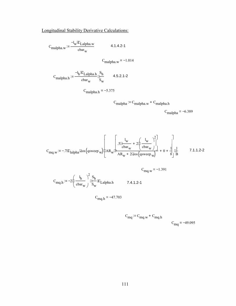
111
Longitudinal Stability Derivative Calculations:
Cmalpha.wlw− CLalpha.w⋅
cbarw:= 4.1.4.2-1
Cmalpha.w 1.014−=
Cmalpha.hlh− CLalpha.h⋅
cbarw
ShSw
⋅:= 4.5.2.1-2
Cmalpha.h 5.375−=
Cmalpha Cmalpha.w Cmalpha.h+:=
Cmalpha 6.389−=
Cmq.w .7− Clalpha⋅ cos qsweep w( )⋅ ARw
.5lw
cbarw⋅ 2
lwcbarw
2
⋅+
ARw 2 cos qsweep w( )⋅+⋅ 0+
18
+
⋅1B
⋅:= 7.1.1.2-2
Cmq.w 1.391−=
Cmq.h 2−lh
cbarw
2
⋅ShSw
⋅ CLalpha.h⋅:= 7.4.1.2-1
Cmq.h 47.703−=
Cmq Cmq.w Cmq.h+:=
Cmq 49.095−=

112
Yaw Moment Stability Derivative Calculations:
Cnbeta.w 0:=at zero lift 5.1.3.1-1
Cybeta.v CLalpha.v−SvSw
⋅:= 5.3.1.1-3
Cnbeta.v Cybeta.v−lvbw
⋅:= 5.6.3.1-1
Cnbeta.v 0.936=
Cnbeta Cnbeta.w Cnbeta.v+:=
Cnbeta 0.936=
Cnr.w 0:=at zero lift 7.1.3.3-2
Cnr.v 2lvbw
2
⋅ Cybeta.v⋅:= 7.4.3.3-1
Cnr.v 2.223−=
Cnr Cnr.w Cnr.v+:=
Cnr 2.223−=

113
Roll Moment Stability Derivative Calculations:
Clr 0.351=
Clr Clr.w Clr.v+:=
Clr.v 0.351=
7.4.3.2 1−Clr.v 2− lv⋅ zv⋅Cybeta.v
bw2
⋅:=
7.1.3.2 1−negligible at zero aoaClr.w 0:=
Clbeta 0.197−=
Clbeta Clbeta.w Clbeta.v+:=
Clbeta.v 0.148−=
at zero aoa 5.3.2.1 2−Clbeta.v Cybeta.vzvbw
⋅:=
Clbeta.w 0.049−=
5.1.2.1 2−at zero aoaClbeta.w gama dihedeff⋅1802
π2
⋅ compcor⋅:=
5.1.2.1 30a−compcor 1.14
+:=
5.1.2.1 29−dihedeff .00015−.00005
3−:=

114
APPENDIX C:
DATCOM CALCULATIONS INCLUDING INTERFERENCE
The following is the MathCAD workspace used to calculate the Datcom estimates
for the stability derivatives including the available interference approximations. The
page numbers for the equations obtained from the Datcom are presented next to the
equation. The subscript w refers to the wing, v refers to the vertical tail, and h refers to
the horizontal tail.

115
Input parameters and initial calculations:
ARhbh
2
Sh:= ARv
bv2
Sv:=ARw
bw2
Sw:=
Clalpha .109180π
⋅:= Clalpha.MaClalpha
B:= 4.1.1.2-1 k
Clalpha.Ma B⋅
2 π⋅:= 4.1.3.2-3
qsweep w 0:= halfsweepw 0:= halfsweeph atan18
:= halfsweepv atan13
:=
CLalpha.wARw 2⋅ π⋅
2 ARwBk
⋅
21
tan halfsweepw( )( )2
B2+
⋅ 4++
:=
4.1.3.2-49
CLalpha.w 4.056=
CLalpha.hARh 2⋅ π⋅
2 ARhBk
⋅
21
tan halfsweeph( )( )2
B2+
⋅ 4++
:=
CLalpha.h 3.23=
Ma .4:= U0 13392Ma⋅:= roe 1.146 10 7−×:=
Sw 16:= Sv 6:= Sh 6:= cbarw 2:= Q .5 roe⋅ U02⋅:= B 1 Ma2−( ).5
:=
bw 8:= bh 4:= bv 3:= zv32
:=
lv 9.5:= lh 8.875:= lw .5:=
gama 5π
180⋅:= zw .5
bw2
sin gama( )2
⋅−:=

116
Longitudinal Stability Derivative Calculations:
Cmq 49.095−=
Cmq Cmq.w Cmq.h+:=Cmq.h 47.703−=
7.4.1.2-1Cmq.h 2−lh
cbarw
2
⋅ShSw
⋅ CLalpha.h⋅:=
Cmq.w 1.391−=
Cmq.w .7− Clalpha⋅cos qsweep w( )
B⋅
ARw .5lw
cbarw⋅ 2
lwcbarw
2
⋅+
⋅
ARw 2 cos qsweep w( )⋅+0+
18
+
⋅:=7.1.1.2-2
Cmalpha 4.304−=
Cmalpha Cmalpha.w Cmalpha.h+:=
Cmalpha.h 3.29−=
Cmalpha.hlh− CLalpha.h⋅
cbarw
Sh 1 down_wash−( )⋅
Sw⋅:=
4.5.2.1-2
4.4.1 7−down_wash .38785:=
Cmalpha.w 1.014−=
4.1.4.2-1Cmalpha.wlw− CLalpha.w⋅
cbarw:=

117
Yaw Moment Stability Derivative Calculations:
Cnr 2.745−=
Cnr Cnr.w Cnr.v+:=
Cnr.v 2.745−=
7.4.3.3-1Cnr.v 2lvbw
2
⋅ Cybeta.v⋅:=
at zero lift 7.1.3.3-2Cnr.w 0:=
Cnbeta 1.156=
Cnbeta Cnbeta.w Cnbeta.v+:=
Cnbeta.v 1.156=
5.6.3.1-1Cnbeta.v Cybeta.v−lvbw
⋅:=
5.3.1.1-3Cybeta.v CLalpha.v−Sv side_wash( )⋅
Sw⋅:=
5.4.1-1side_wash .724 3.06
SvSw
1 cos qsweep w( )+
⋅+ 0+ .009 ARw⋅+:=
CLalpha.vARv.eff 2⋅ π⋅
2 ARv.effBk
⋅
21
tan halfsweepv( )( )2
B2+
⋅ 4++
:=
ARv.eff 1.365=
5.3.1.1-2ARv.eff body intfer ARv⋅ 1 KH htailintfer 1−( )⋅+ ⋅:=
5.3.1.1-22KH .9:=htailintfer .9:=body intfer 1:=
at zero lift 5.1.3.1-1Cnbeta.w 0:=

118
Roll Moment Stability Derivative Calculations:
Clr 0.433=
Clr Clr.w Clr.v+:=
Clr.v 0.433=
7.4.3.2 1−Clr.v 2− lv⋅ zv⋅Cybeta.v
bw2
⋅:=
7.1.3.2 1−negligible at zero aoaClr.w 0:=
Clbeta 0.231−=
Clbeta Clbeta.w Clbeta.v+:=
Clbeta.v 0.183−=
at zero aoa 5.3.2.1 2−Clbeta.v Cybeta.vzvbw
⋅:=
Clbeta.w 0.049−=
5.1.2.1 2−at zero aoaClbeta.w gama dihedeff⋅1802
π2
⋅ compcor⋅:=
5.1.2.1 30a−compcor 1.14
+:=
5.1.2.1 29−dihedeff .00015−.00005
3−:=

VITA
Deric Austin Babcock
Candidate for the Degree of
Master of Science
Thesis: AIRCRAFT STABILITY DERIVATIVE ESTIMATION FROM FINITE ELEMENT ANALYSIS
Major Field: Aerospace Engineering
Biographical:
Personal Data: Born in Kingfisher, Oklahoma on July 21, 1980, the son of Larry R. Babcock and Sandra G. Babcock.
Education: Graduated from Lone Grove High School, Lone Grove Oklahoma, in
May 1998; received Bachelor of Science degree majoring in Mechanical and Aerospace Engineering from Oklahoma State University, Stillwater, Oklahoma, in May 2002; completed the requirements for the Master of Science degree in Mechanical Engineering at Oklahoma State University in July 2004.
Experience: Tutor, Mathematics Learning Resource Center, 1999-2001; Teaching
Assistant, OSU Mechanical and Aerospace Engineering Department, 2002-2004; Research Assistant, OSU MAE Dept. 2003-2004.
Professional Memberships: American Institute of Aeronautics and Astronautics,
American Society of Mechanical Engineers, Sigma Gamma Tau.