Introduction

By its contribution in Document 1C/140 of 16 March 2015, the Russian Federation proposed changes to the text of Report ITU-R SM.2256, on spectrum occupancy measurements and evaluation, aimed to bringing greater clarity to a rather complicated sphere concerning the accuracy and reliability of spectrum occupancy measurements and evaluation. At its June 2015 meeting, WP 1C endorsed the said proposals in principle, publishing them as Document 1C/169, Annex 1, for discussion at the forthcoming WP 1C meeting in June 2016, while at the same time proposing that the provisions in Report ITU-R SM.2256 relating to lock-in and lock-out measuring systems be clarified. Additional studies in that regard have shown the following: According to Recommendation ITU-R SM.1880-1, on spectrum occupancy measurement and evaluation, the number of samples required for calculating spectrum occupancy with the requisite accuracy is, in the case of pulsed signals, markedly higher than the number of samples required for lengthy signals, in which regard a subsection on lock-in and lock-out measuring systems was included in Report ITU-R SM.2256. Therefore, in a situation – frequently encountered in practice – of a priori uncertainty as to the nature (pulsed or lengthy) of the signal to be measured, the number of samples has to be selected on the basis of the requirements with respect to the specified accuracy and reliability of the spectrum occupancy measurement in the presence of pulsed signals. Therefore, it can be considered that for lengthy signals these requirements will automatically be met, and by a wide margin. With this understanding, the relatively small difference in the number of samples required for the qualitative measurement of spectrum occupancy where lengthy signals are present and measured using lock-in and lock-out measuring systems is insignificant. In the interests of simplifying Report ITU-R SM.2256, therefore, it is altogether feasible to dispense with dividing the conditions for measuring channel occupancy with lengthy signals into measurements using lock-in or lock-out measuring systems, and to perform the entire analysis with reference to lock-out systems, which are more widely used in practice. In developing the proposals for revising the text of Report ITU-R SM.2256 that are set forth in Document 1C/140 of 16 March 2015 (and also reflected in Annex 1 to Document 1C/169 of 19 June 2015), in order to ensure consistency between the new and existing materials, there has been some rearrangement of individual segments of the existing text of Report ITU-R SM.2256.

Radiocommunication Study Groups

Received: 28 January 2015

Subject: Report ITU-R SM.2256 Annex 1 to Document 1C/169, dated 19.06.2015

Document 1C/6-E 16 February 2016 Original: Russian

Russian Federation

PROPOSALS FOR A REVISION OF REPORT ITU-R SM.2256

Spectrum occupancy measurements and evaluation

- 2 - 1C/6-E

The removal from Report ITU-R SM.2256 of the subsection concerning measurements using lock-in and lock-out systems calls for some rearrangements in other parts of the text. In order to make the proposals more clear, the best option is, therefore, not to present them in the form of further changes to Document 1C/169, Annex 1, but directly within the body of Report ITU-R SM.2256, and this is the form in which they are presented in this contribution.

Proposal

The proposed draft revision of Report ITU-R SM.2256 is set forth in the attachment hereto.

- 3 - 1C/6-E

ATTACHMENT

DRAFT REVISION OF REPORT ITU-R SM.2256-0

Spectrum occupancy measurements and evaluation (2012)

Summary

Spectrum occupancy measurements and evaluation in modern RF environments with increasing density of digital systems and frequency bands shared by different radio services become a more and more complex and challenging task for Monitoring Services. Based on Recommendations ITU-R SM.1880, ITU-R SM.1809, and information provided in the 2011 Edition of the ITU Handbook on Spectrum Monitoring, this draft new Report provides a far more detailed discussion on different approaches to spectrum occupancy measurements, possible issues related to them and their solutions.

TABLE OF CONTENTS Page

1 Introduction ...................................................................................................... 4

2 Terms and definitions ....................................................................................... 5

2.1 Spectrum resource ............................................................................................ 5

2.2 Frequency channel occupancy measurement ................................................... 5

2.3 Frequency band occupancy measurement ........................................................ 5

2.4 Measurement area ............................................................................................. 5

2.5 Duration of monitoring (TT) ............................................................................. 6

2.6 Sample measurement time (TM) ........................................................................ 6

2.7 Observation time (TObs) .................................................................................... 6

2.8 Revisit time (TR) ............................................................................................... 6

2.9 Occupancy time (TO) ........................................................................................ 6

2.10 Integration time (TI) .......................................................................................... 7

2.11 Maximum number of channels (NCh) ................................................................ 7

2.12 Transmission length .......................................................................................... 7

- 4 - 1C/6-E

2.13 Threshold .......................................................................................................... 7

2.14 Busy hour .......................................................................................................... 7

2.15 Access delay ..................................................................................................... 7

2.16 Frequency channel occupancy (FCO) .............................................................. 7

2.17 Frequency band occupancy (FBO) ................................................................... 8

2.18 Spectrum resource occupancy (SRO) ............................................................... 8

3 Measurement parameters .................................................................................. 10

3.1 Selectivity ......................................................................................................... 10

3.2 Signal to noise ratio .......................................................................................... 11

3.3 Dynamic range .................................................................................................. 12

3.4 Threshold .......................................................................................................... 12

3.4.1 Pre-set threshold ............................................................................................... 12

3.4.2 Dynamic threshold ............................................................................................ 13

3.5 Measurement timing ......................................................................................... 15

3.6 Directivity of the measurement antenna ........................................................... 17

4 Site considerations ............................................................................................ 18

5 Measurement procedure ................................................................................... 20

5.1 FCO measurement with a scanning receiver .................................................... 20

5.2 FBO with a sweeping analyser ......................................................................... 20

5.3 FBO with FFT methods .................................................................................... 20

6 Calculation of occupancy ................................................................................. 21

6.1 Combining measurement samples on neighbouring frequencies ..................... 21

6.2 Classifying emissions in bands with different channel widths ......................... 22

7 Presentation of results ....................................................................................... 23

7.1 Traffic on a single channel ............................................................................... 23

7.2 Occupancy on multiple channels ...................................................................... 24

7.3 Frequency band occupancy .............................................................................. 26

- 5 - 1C/6-E

7.4 Spectrum resource occupancy .......................................................................... 28

7.5 Availability of results ....................................................................................... 29

8 Special occupancy measurements .................................................................... 29

8.1 Frequency channel occupancy in frequency bands allocated to point-to-point systems of fixed service .................................................................................... 29

8.2 Separation of occupancy for different users in a shared frequency resource ... 30

8.3 Spectrum occupancy measurement of WLAN (Wireless Local Area Networks) in 2.4 GHz ISM band ........................................................................................ 31

8.4 Determining the necessary channels for the transition from analogue to digital trunked systems ................................................................................................ 32

8.5 Estimation of RF use by different radio services in shared bands .................... 35

9 Uncertainty considerations ............................................................................... 35

10 Interpretation and usage of results .................................................................... 36

10.1 General .............................................................................................................. 36

10.2 Interpretation of occupancy results in shared channels .................................... 36

10.3 Using occupancy data to assess spectrum utilization ....................................... 36

11 Conclusions ...................................................................................................... 37

Annex 1 – Probabilistic approach to spectrum occupancy measurements and relevant measurement data handling procedures ............................................................ 38

A Preface .............................................................................................................. 38

A1 General description of the approach ................................................................. 38

A2 Concept of spectrum occupancy ....................................................................... 39

A2.1 Spectrum occupancy as a statistical concept .................................................... 39

A2.2 Occupancy measurement error ......................................................................... 40

A2.3 Accuracy and confidence level of occupancy measurement ............................ 41

A2.4 Parameters affecting the statistical confidence of occupancy measurement .... 42

A2.4.1 Pulsed and lengthy signals and signal flow rate. ........................................... 42

A2.4.2 Relative instability of revisit time ................................................................. 43

- 6 - 1C/6-E

A2.4.3 Use of lock-in and lock-out measuring systems for occupancy measurements ................................................................................................ 43

A3 Measuring procedures ....................................................................................... 44

A3.1 Recommendations for measuring occupancy with lock-in measuring systems on radio channels with lengthy signals ............................................................. 44

A3.1.1 Data collection and occupancy measurement rule for the case of small instability of the revisit time ............................................................... 44

A3.1.2 Occupancy measurement rule Data collection and occupancy measurement rule for the case of meaningful instability of the revisit time ........................ 44

A3.1.3 Selecting the number of samples on the base of the expected signal flow rate ......................................................................................................... 44

A3.1.4 Effect of incorrect choice of number of samples on the confidence level of the occupancy measurement ................................................................ 47

A3.2 Recommendations for measuring occupancy with lock-out measuring systems Recommendations for measuring occupancy on radio channels with pulsed signals .................................................................................................... 48

A3.2.1 Data collection and occupancy measurement rule ........................................ 48

A3.2.2 Occupancy calculation rule ........................................................................... 49

A3.2.32 Selecting the number of samples on the base of the expected occupancy level ............................................................................................................. 49

A3.3 Selecting the number of samples in the absence of a prior information on an occupancy level ................................................................................................ 49

A3.4 Effect of reduced a smaller number of samples on confidence level and the occupancy measurement error ............................................................................................ 49

A4 Typical examples of the impact of signal flow rate in the radio channel on the confidence level of spectrum occupancy calculations ........................... 49

A4.1 Case A: One single signal present in the integration time ................................ 49

A4.2 Case B: Twelve signals during the integration time ......................................... 50

A4.3 Case C: Several dozen signals within the integration time .............................. 50

Reference to Annex A ................................................................................................ 51

- 7 - 1C/6-E

No changes from ‘‘ Introduction’’ to section A2.4.2 « Relative instability of revisit time» of Annex 1 to the Report (inclusive)

A2.4.3 Use of lock-in and lock-out measuring systems for occupancy measurements In the case of unstable revisit times, the confidence level of occupancy measurements depends also on whether the measuring system used is a lock-in or a lock-out system. Lock-in systems feature is the use of a generator, which determines a kind of ideal grid of sampling points on the time axis. The real channel state samples may be displaced in relation to the nodes of this ideal grid, but for points located in the different sections of the integration time these displacements are independent. Lock-out systems are understood to be ones in which there is no time grid, measurement is carried out on the basis of approximately equal revisit times, and the displacement of any point affects the placement on the time axis of all subsequent sampling points. For short time intervals, the difference in the systems’ behaviour is not too noticeable, but for a typical integration time duration TI of hundreds of seconds, the differences in the placement of channel state samples on the time axis become significant and have a noticeable impact on the statistical characteristics of occupancy measurement in radio channels with lengthy signals. Recommendations for achieving measurement confidence for lock-in and lock-out systems will be given in the next sections. Statistically confident measurement of occupancy in channels with pulse signals requires a much larger number of samples in the integration time, although for pulse signals the difference between lock-in and lock-out systems becomes negligible.

A3 Measuring procedures

A3.1 Recommendations for measuring occupancy with lock-in measuring systems on radio channels with lengthy signals

A3.1.1 Data collection and occupancy measurement rule for the case of small instability of the revisit time

To measure occupancy, one must at the very least determine for each integration time the number JO of occupied channel state samples. With the relative instability δT of an interval between repeated measurements, not exceeding units of a percent, during data collection for each time period of integration TI , it is sufficient to fix quantity of samples related to the occupied state of a channel JO among total number of samples of the channel state JI. Where there are predominantly lengthy signals in the channel, in order to ensure measurement confidence, information is also required on the signal flow rate λ. When such information is lacking, it is worthwhile to track the grouping of occupied and free states so as to determine a quantity Vr of signals detected in the channel in the r-th integration time. The number of signals detected Vr is considered to be equal to the number of changeovers from free to occupied state and vice versa.

A3.1.2 Occupancy measurement rule The rule for the measurement of occupancy was already discussed earlier in § A2.2, and takes the form:

Io JJSOCR = (A7)

where: SOCR : spectrum occupancy calculation result

- 8 - 1C/6-E

JO : number of occupied channel states detected during the integration time JI : total number of channel state samples throughout of the integration time. Where there are predominantly lengthy signals in the channel, in order to ensure measurement confidence, information is also required on the signal flow rate λ. When such information is lacking, it is worthwhile to track the grouping of occupied and free states so as to determine a quantity Vr of signals detected in the channel in the r-th integration time. The number of signals detected Vr is considered to be equal to the number of changeovers from free to occupied state and vice versa.

A3.1.2 Data collection and occupancy measurement rule for the case of meaningful instability of the revisit time

At an instability δT exceeding 10 %, instead of the number of samples it is necessary to record the actual integration time TAI and the aggregate length of time spent by the channel in occupied state TO. At the start of the measurements, one should set TAI = 0 and TO = 0 and determine the channel state corresponding to time t0. After each subsequent observation, the value TAI should be increased up to the duration of the revisit time tR j determined by equation (A4):

jRAIAI TjTjT += )1–()( (A8)

If the channel state was occupied at both sampling points tj-1 and tj, then TO should be also increased up to the same increment:

jRoo TjTjT += )1–()( (A9)

If within the interval TR j a change in channel state is observed then only a half of the revisit time should be included as an occupied state duration:

2/)1–()( jRoo TjTjT += (A10)

And if the channel is observed to be in passive state at both sampling points the occupied state length TO should be left unchanged. The rule for calculating occupancy takes the form:

AIo TTSOCR = (A11)

where: SOCR : spectrum occupancy calculation result

TO : aggregate length of time spent by the channel in occupied state TAI : length of the actual integration time. In order to determine the confidence level of the measurements one should record the quantity of signals observed over the occupancy integration time (see § A3.1.1).

- 9 - 1C/6-E

A3.1.3 Selecting the number of samples on the base of the expected signal flow rate Requirements for measuring equipment and for relevant data handling processes of occupancy calculations will be different for channels with lengthy and pulsed signals. For channels with lengthy signals, it is determined first of all by the quantity of signals within the integration time. For channels occupied by pulsed signals, confidence depends on the value of radio channel occupancy itself (see § A3.2.2 below). For radio channels with lengthy signals, the number of samples required to achieve a confidence PSOC with a permissible absolute measurement error tolerance ΔSO may be calculated as follows:

( )

206.1 2

minTVx

J avr

SO

pI

d+××

D= (A8A12)

where: JI min : recommended required (minimum necessary) number of samples ΔSO : maximum permissible absolute measurement error, corresponding to half of

the confidence interval δT : relative instability of revisit time Vavr : average number of signals expected within the occupancy integration time xP : percentage point of the probability integral, corresponding to the required

confidence value PSOC, for the calculation of which the following approximation can be recommended.

)04481.099229.0(1

27061.030753.2–×+×+

×+=

yyyyxp (A9A13)

where:

÷ø

öçè

æ×=

SOCPlny

–122 (A10A14)

The average number Vavr of signals expected within the integration time used in (A8A12) can be predicted as:

Iavr TV ×l= (A11A15)

where: λ : signal flow rate in the channel (see § A2.4.1) TI : duration of the occupancy integration time. For a confidence level PSOC = 95% with a permissible absolute measurement error tolerance ΔSO = 0.5% equation (A8A12) for lock-in systems can be represented as:

( )2min 06.12.194 TVJ avrI d+××= (A12A16)

- 10 - 1C/6-E

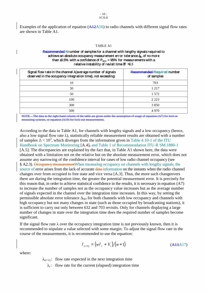
Examples of the application of equation (A12A16) to radio channels with different signal flow rates are shown in Table A1.

TABLE A1

Recommended Nnumber of samples for a channel with lengthy signals required to achieve an absolute occupancy measurement er ror tolerance ΔSO of no more

than ±0.5% with a confidence of PSOC = 95% for measurements with a relative instability of revisit time δT ≤ 0.5

Signal flow rate in the channel λ (average number of signals observed in the occupancy integration time), not exceeding:

Recommended Required number of samples

10 703 30 1 217 50 1 572

100 2 223 300 3 850 500 4 970

NOTE – The data in the right-hand column of the table are given under the assumption of usage of equation (A7) for lock-in measuring systems, or equation (A19) for lock-out measurements.

According to the data in Table A1, for channels with lengthy signals and a low occupancy (hence, also a low signal flow rate λ), statistically reliable measurement results are obtained with a number of samples JI < 103, which diverges from the information given in Table 4.10-1 of the ITU Handbook on Spectrum Monitoring [A.4], and Table 1 of Recommendation ITU-R SM.1880-1 [A.5]. The discrepancies are explained by the fact that, in Table A1 shown here, the data were obtained with a limitation not on the relative but on the absolute measurement error, which does not assume any narrowing of the confidence interval for cases of low radio channel occupancy (see § A2.3). Occupancy measurementWhen measuring occupancy on channels with lengthy signals, the source of error arises from the lack of accurate data information on the instants when the radio channel changes over from occupied to free state and vice versa [A.3]. Thus, the more such changeovers there are during the integration time, the greater the potential measurement error. It is precisely for this reason that, in order to achieve statistical confidence in the results, it is necessary in equation (A7) to increase the number of samples not as the occupancy value increases but as the average number of signals expected in the channel over the integration time increases. In this way, by setting the permissible absolute error tolerance ΔSO for both channels with low occupancy and channels with high occupancy but not many changes in state (such as those occupied by broadcasting stations), it is sufficient to carry out only between 632 and 703 revisits. Only for channels displaying a large number of changes in state over the integration time does the required number of samples become significant. If the signal flow rate λ over the occupancy integration time is not previously known, then it is recommended to stipulate a value selected with some margin. To adjust the signal flow rate in the course of the measurements, it is recommended to use the equation:

( ) ( )1)1( ++=+ wVw rrr ll (A13A17)

where: λ(r+1) : flow rate expected in the next integration time λr : flow rate for the current (elapsed) integration time

- 11 - 1C/6-E

Vr : number of signals that has been determined in the current integration time w : weighting coefficient determining the response time of the adaptation

procedure, usually selected within the range 5 ≤ w < 20. To start the evolution according to equation (A13A17) an initial value λ0 is needed which is usually unknown a priori. It is advisable to choose a maximum among all values expected within the given frequency range, which corresponds to the worse case. For channels with pulsed signals, calculation (A7) also gives an unbiased occupancy measurement but it requires significantly more samples to achieve a confidence PSOC with a permissible absolute measurement error tolerance ΔSO . We can calculate the necessary number of samples JIT as:

2

min )–1( ÷÷ø

öççè

æD

××=SO

pI

xSOSOJ

2

min )–1( ÷÷ø

öççè

æD

××=SO

pI

xSOSOJ (A14)

where: JI min :recommended (minimum necessary) number of samples SO :radio channel occupancy for the channel with pulse signals xP :percentage point of the probability integral (see (A9)) ΔSO : maximum permissible absolute measurement error, corresponding to half of the

confidence interval. For a confidence level PSOC = 95% and a maximum permissible absolute measurement error ΔSO = 0.5% equation (A14) can be expressed as follows:

)–1(664153min SOSOJ I ××= )–1(664153min SOSOJ I ××= (A15)

With pulse-type signals, the confidence of the calculation (A7) is determined by the occupancy value itself and is practically independent of instability of samples placement along the time axis and also of whether the measurements involved are of the lock-in or lock-out variety. The application of equation (A15) to radio channels with different occupancies is illustrated in Table A2.

A3.1.4 Effect of incorrect choice of number of samples on the confidence level of the occupancy measurement

Reducing the number of samples JI by a factor of K in relation to what is recommended in Tables A1 and A2 will reduce reliability, or widen the confidence interval proportionally with K. Let us assume, for example, that we need to measure the occupancy of a radio channel with a signal flow rate of no more than 50 signals within the integration time. From the last column in Table A1, we see that the recommendation in this case is to sample the channel state 1 572 times. Complying with this recommendation, the occupancy calculation (A7) will deviate by no more than ΔSO = 0.5% from the real value, with a confidence level of PSOC = 95%. If we now assume, on the other hand, that the system is actually capable of taking only 393 channel state samples over the integration time, i.e. four times less than the recommended number, then on average the occupancy will as before be measured accurately, but the range within which the real occupancy value will occur with a confidence level of 95% is increased fourfold to ±2% either side of the measurement result.

- 12 - 1C/6-E

An inadequate number of samples JI may also be observed when data collection for the occupancy calculation is curtailed prematurely. In such cases, the occupancy calculation (A7) remains unbiased but the confidence level of the results is diminished similarly to the example discussed above.

TABLE A2

Recommended number of samples for a channel with pulse signals, required to achieve an absolute occupancy measurement er ror tolerance ΔSO of no

greater than ±0.5% with a confidence of PSO = 95%

Radio channel occupancy SO (%)

Recommended number of samples, JI

Recommended revisit time, TR (ms)

for TI = 5 minutes for TI = 15 minutes

5 7 300 41.1 123.2 10 13 830 21.7 65.0 20 24 586 12.2 36.6 35 34 960 8.6 25.7 50 38 416 7.8 23.4

NOTE – The required number of samples for channels with an occupancy SO* > 50% coincides with the number of samples for an occupancy SO = 1 − SO*. In other words, for instance, to achieve statistically confident measurements in a channel with an occupancy of 80% it is necessary to select JI = 24 586, as in the case of occupancy SO = 1 − 0.80 = 20%.

A3.2 Recommendations for measuring occupancy with lock-out measuring systems Relationship (A7) may be used to calculate occupancy in lock-out systems too, but the statistical confidence of the occupancy calculation in such systems deteriorates noticeably as the relative instability δT increases. Calculation quality can be improved by accurately determining the moments in time at which the radio channel state is tested. Broadly speaking, the measurements should not verify the number of occurrences of occupied and free states in the channel, but rather the length of time the channel spends in occupied or free state.

A3.2.1 Data collection To calculate occupancy, it is necessary as a minimum, in each integration time, to record the actual integration time TAI and the aggregate length of time spent by the channel in occupied state TO. At the start of the measurements, one should set TAI = 0 and TO = 0 and determine the channel state corresponding to time t0. After each subsequent observation, the value TAI should be increased up to the duration of the revisit time tR j determined by equation (A4):

jRAIAI TjTjT += )1–()( (A16)

If the channel state was occupied at both sampling points tj-1 and tj, then TO should be also increased up to the same increment:

jRoo TjTjT += )1–()( (A17)

- 13 - 1C/6-E

If within the interval TR j a change in channel state is observed then only a half of the revisit time should be included as an occupied state duration:

2/)1–()( jRoo TjTjT += (A18)

And if the channel is observed to be in passive state at both sampling points the occupied state length TO should be left unchanged. In order to verify the confidence level of the measurements, as it was done with lock-in systems, one should record the quantity of signals observed over the occupancy integration time (see §§ A3.1.1 and A3.1.3).

A3.2.2 Occupancy calculation rule The rule for calculating occupancy takes the form:

AIo TTSOCR = (A19)

where: SOCR : spectrum occupancy calculation result

TO : aggregate length of time spent by the channel in occupied state TAI : length of the actual integration time.

A3.2.3 Selecting the number of samples Determining the length of time during which occupied state is observed in the channel prevents the accumulation of error which is typical for lock-out measurements. As a result, the statistical characteristics of equation (A19) for lock-out measuring systems coincide with the quality obtained in equation (A7) for lock-in systems. This means that the number of samples required to achieve a confidence level PSOC = 95% may be calculated using rules (A7) and (A19) above or read off from Tables A1 and A2. Using equation (A7) for lock-out measurements is in principle acceptable, but the quantity of samples required to achieve measurement confidence rises sharply as the relative instability of the revisit time increases.

A3.2 Recommendations for measuring occupancy on radio channels with pulsed signals

A3.2.1 Data collection and occupancy measurement rule To measure occupancy, one must at the very least determine for each integration time the number JO of occupied channel state samples. For channels with pulsed signals, calculation (A7) also gives an unbiased occupancy measurement but it requires significantly more samples to achieve a confidence PSOC with a permissible absolute measurement error tolerance ΔSO .

A3.2.2 Selecting the number of samples on the base of the expected occupancy level When measuring occupancy on channels with pulsed signals we can calculate the necessary number of samples JImin as:

- 14 - 1C/6-E

2

min )–1( ÷÷ø

öççè

æD

××=SO

pI

xSOSOJ

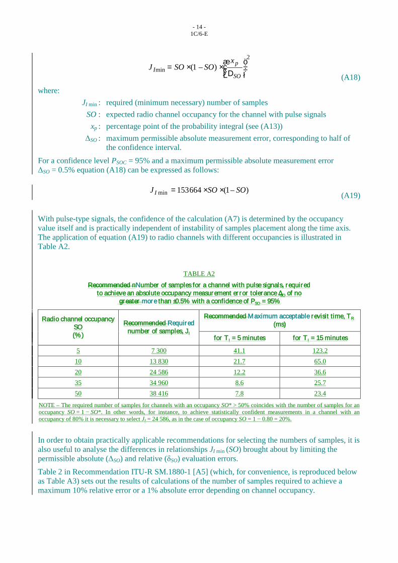
(A18) where: JI min : required (minimum necessary) number of samples SO : expected radio channel occupancy for the channel with pulse signals xp : percentage point of the probability integral (see (A13)) ΔSO : maximum permissible absolute measurement error, corresponding to half of

the confidence interval. For a confidence level PSOC = 95% and a maximum permissible absolute measurement error ΔSO = 0.5% equation (A18) can be expressed as follows:

)–1(664153min SOSOJ I ××= (A19)

With pulse-type signals, the confidence of the calculation (A7) is determined by the occupancy value itself and is practically independent of instability of samples placement along the time axis. The application of equation (A19) to radio channels with different occupancies is illustrated in Table A2.

TABLE A2

Recommended nNumber of samples for a channel with pulse signals, required to achieve an absolute occupancy measurement er ror tolerance ΔSO of no

greater more than ±0.5% with a confidence of PSO = 95%

Radio channel occupancy SO (%)

Recommended Required number of samples, JI

Recommended Maximum acceptable revisit time, TR (ms)

for TI = 5 minutes for TI = 15 minutes

5 7 300 41.1 123.2 10 13 830 21.7 65.0 20 24 586 12.2 36.6 35 34 960 8.6 25.7 50 38 416 7.8 23.4

NOTE – The required number of samples for channels with an occupancy SO* > 50% coincides with the number of samples for an occupancy SO = 1 − SO*. In other words, for instance, to achieve statistically confident measurements in a channel with an occupancy of 80% it is necessary to select JI = 24 586, as in the case of occupancy SO = 1 − 0.80 = 20%.

In order to obtain practically applicable recommendations for selecting the numbers of samples, it is also useful to analyse the differences in relationships JI min (SO) brought about by limiting the permissible absolute (ΔSO) and relative (δSO) evaluation errors. Table 2 in Recommendation ITU-R SM.1880-1 [A5] (which, for convenience, is reproduced below as Table A3) sets out the results of calculations of the number of samples required to achieve a maximum 10% relative error or a 1% absolute error depending on channel occupancy.

- 15 - 1C/6-E

As can be seen from the table, a fixed (10%) limitation of the relative error for small occupancy values (lower than 5%) will lead to a significant increase in the required number of samples owing to the fact that, in this case, the resulting absolute error is very small. At the same time, ensuring a comparable degree of accuracy for large (over 30%) occupancy values calls for a very small number of samples. In contrast, a fixed (1%) limitation of the absolute error will lead to an increase in the required number of samples for large (greater than 20%) occupancy values, since in this case the resulting relative error displays low values. At the same time, ensuring such a degree of accuracy for an occupancy of less than 3% calls for a small number of samples. In order to reduce the required number of samples over the entire range of occupancy variations, a possible solution is to make an estimate while, for large occupancy values, customarily limiting the permissible relative error, and, for small values, limiting the permissible absolute error [A.6]. If the transition from one type of limitation to the other is effected at the 10% occupancy level, the required number of samples will be determined by the values shown in bold type in Table A3, which is entirely acceptable from the practical standpoint.

TABLE A3

Number of samples required to achieve a maximum 10% relative er ror δSO or a 1% absolute er ror ΔSO with a 95% confidence level

Channel occupancy,

%

Required relative er ror δSO = 10% Required absolute er ror ΔSO = 1%

Resulting magnitude of

absolute er ror , %

Required number of independent

samples

Resulting magnitude of

relative er ror , %

Required number of independent

samples

1 0.1 38 047 100.0 380 2 0.2 18 832 50.0 753 3 0.3 12 426 33.3 1 118 4 0.4 9 224 25.0 1 476 5 0.5 7 302 20.0 1 826

10 1.0 3 461 10.0 3 461 15 1.5 2 117 6.7 4 900 20 2.0 1 535 5.0 6 149 30 3.0 849 3.3 8 071 40 4.0 573 2.5 9 224 50 5.0 381 2.0 9 608 60 6.0 253 1.7 9 224 70 7.0 162 1.4 8 071 80 8.0 96 1.3 6 149 90 9.0 43 1.1 3 459

With this approach, the relative evaluation error increases for small occupancy values; however, from the practical standpoint, this can be entirely acceptable since the absolute evaluation error will then be small. Thus, for a 2% occupancy, the boundaries of the confidence interval at 1% and 3% corresponding to a 50% relative evaluation error nevertheless characterize an extremely low channel occupancy, making it hardly worthwhile to expend considerable additional computing resources to confirm this obvious fact with an additional accuracy amounting to no more than a few tenths of a per cent.

- 16 - 1C/6-E

The meaning of the required number of samples as shown in bold type in Table A3 can be explained as follows. Where a channel for which there is no prior occupancy information is evaluated on the basis of 1 000 samples, the measurement accuracy for occupancy values in the order of 27% and 3% will be approximately as shown in Table A3, i.e. an approximate 10% relative error for 27% occupancy and an approximate 1% absolute error for 3% occupancy. Occupancy values greater than 27% will be measured with a relative error of less than 10%, while occupancy values lower than 3% will be measured with an absolute error of less than 1%. For radio channels with an occupancy from 3% to 27%, measurements will be characterized by a relative error exceeding 10% and an absolute error exceeding 1%. Thus, adopting an approach to evaluating spectrum occupancy measurement quality for small occupancy values based on permissible absolute error simply implies accepting the possibility of increased relative measurement error for such small occupancy values, recognizing that the absolute error values remain small.

3.3 Selecting the number of samples in the absence of a prior information on an occupancy level

By analysing the dependencies, shown in Table A3, between the required number of samples and channel occupancy, it is easy to observe that among the values shown in bold type the most significant (3 461) corresponds to an occupancy of 10%. This means that by selecting, to be on the safe side, a somewhat higher value, for example 3 600 samples (corresponding to a sampling rate of four times per second over a period of 15 minutes), this can be used as the single universal number of samples for the entire range of occupancy variation from 1% (and below) to 100%. The measurement error will then be lower than 10% of the relative error for channels with an occupancy exceeding 10%, and lower than 1% of the absolute error for channels with an occupancy of less than 10%. A decrease in occupancy (from 10%) will be accompanied by a consequential decrease in the absolute estimation error, while an increase in occupancy (relative to 10%) will be accompanied by a consequential decrease in the relative error. Specific calculated values for the resulting errors are shown in bold type on the left-hand side of Table A4.

TABLE A4

Occupancy measurement er rors cor responding to a 95% confidence level, achievable when estimating occupancy with exactly 3 600 and 1 800 data samples

Occupancy, % Number of samples: 3 600 Number of samples: 1 800

Resulted absolute er ror , %

Resulted relative er ror , %

Resulted absolute er ror , %

Resulted relative er ror , %

1 0.33 32.5 0.46 46.0 2 0.46 22.9 0.65 32.3 3 0.56 18.6 0.79 26.3 4 0.64 16.0 0.91 22.6 5 0.71 14.2 1.01 20.1

10 0.98 9.8 1.39 13.9 15 1.17 7.8 1.65 11.0 20 1.31 6.5 1.85 9.2 30 1.50 5.0 2.12 7.1 40 1.60 4.0 2.26 5.7

- 17 - 1C/6-E

50 1.63 3.3 2.31 4.6 60 1.60 2.7 2.26 3.8 70 1.50 2.1 2.12 3.0 80 1.31 1.6 1.85 2.3 90 0.98 1.1 1.39 1.5

In the vast majority of cases, it is entirely possible to use half the number of samples, i.e. 1 800 samples, as a single universal number, corresponding to a sampling rate of twice per second over a period of 15 minutes, thereby allowing for the use of slower equipment. The calculated values of the resulting errors for 1 800 samples are shown on the right-hand side of Table A4. Where 1 800 samples are used instead of 3 600, the absolute estimation errors increase by a factor of 41.12 » , while exceeding by a relative error of 10% for small occupancy values begins not at 10% but at 14%. Nevertheless, with 1 800 samples, the corresponding absolute error values remain relatively small, differing from the 3 600 case only by tenths of a per cent, this being altogether acceptable for practical purposes. Besides, as can be seen from Fig. 1 in Recommendation ITU-R SM.1880-1 [A.5], the resulting relative error values for 1 800 samples do not lie within the no-go area, confirming their acceptability. Thus, in the absence of a prior data on an occupancy level in an analyzed radio channel it is recommended to make a primary occupancy estimation on the basis of an universal sample number, equal 3600 (or 1800 samples in the case of the low-speed radio monitoring equipment) and then, if it is necessary to provide more accurate measurements, to rectify requirements to the sample number on the basis of the obtained SO value and recommendations of § A3.2.2, and to repeat the calculations with this sample number. As already mentioned above, the values shown in Table A4 correspond to the occupancy measurement of channels with pulsed signals. For channels with lengthy signals, the absolute estimation errors are inversely proportional to the number of processed samples and, as can be seen in Fig. A3, can be significantly smaller than for pulsed signals. Where it is a known fact that precisely such signals are occurring within the channel, the number of samples can be reduced to 600, as can be seen from the data in Table A5, which presents the calculated values of the relative and absolute errors according to channel occupancy and the ratio τs / TI, where τs is the duration of each lengthy signal, which are considered to be equal in the model used, and TI is the integration time. From Table A5 it can be seen that the measurement errors diminish considerably as the relative duration of lengthy signals increases.

TABLE A5

Error cor responding to the confidence level of 95% observed when estimating occupancy in a channel with lengthy signals of a duration not less than the specified value of the

ratio τs / TI for 600 data samples

Channel occupancy,

%

τs / TI = 0.0025 τs / TI = 0.01

Resulted absolute er ror , %

Resulted relative er ror , %

Resulted absolute er ror , %

Resulted relative er ror , %

1 0.34 33.64 0.17 16.82 2 0.48 23.79 0.24 11.89 3 0.58 19.42 0.29 9.71 4 0.67 16.82 0.34 8.41

- 18 - 1C/6-E

5 0.75 15.04 0.38 7.52 10 1.06 10.64 0.53 5.32 15 1.30 8.69 0.65 4.34 20 1.50 7.52 0.75 3.76 30 1.84 6.14 0.92 3.07 40 2.13 5.32 1.06 2.66 50 2.38 4.76 1.19 2.38 60 2.61 4.34 1.30 2.17 70 2.81 4.02 1.41 2.01 80 3.01 3.76 1.50 1.88 90 3.19 3.55 1.60 1.77

FIGURE A3

Absolute er ror ΔSO of a spectrum occupancy estimate with a 95% confidence level, in the case of 1 800 samples for pulsed signals in channel (1), or 500 (2), 250 (3), 100 (4) or 30 (5)

lengthy signals in the channel over the integration time

A3.1.4 Effect of incorrect choice of reduced number of samples on the confidence level of and the occupancy measurement error

Reducing the number of samples JI by a factor of K in relation to what is recommended in Tables A1 and A2 to A3 will reduce reliability, or widen the confidence interval proportionally with K. Let us assume, for example, that we need to measure the occupancy of a radio channel with a signal flow rate of no more than 50 signals within the integration time. From the last column in Table A1, we see that the recommendation in this case is to sample the channel state 1 572 times. Complying with this recommendation, the occupancy calculation (A7) will deviate by no more than ΔSO = 0.5% from the real value, with a confidence level of PSOC = 95%. If we now assume, on the other hand, that the system is actually capable of taking only 393 channel state samples over the integration time, i.e. four times less than the recommended number, then on average the occupancy will as

- 19 - 1C/6-E

before be measured accurately, but the range within which the real occupancy value will occur with a confidence level of 95% is increased fourfold to ±2% either side of the measurement result. An inadequate A reduced number of samples JI may also be observed when data collection for the occupancy calculation is curtailed prematurely. In such cases, the occupancy calculation (A7) remains unbiased but the confidence level of the results is diminished similarly to the example discussed above.

A4 Typical examples of the impact of signal flow rate in the radio channel on the confidence level of spectrum occupancy calculations

Next examples testify the importance of tracking signal flow rate in radio channels where the aim is to obtain occupancy measurements with a high degree of accuracy and statistical confidence. Occupancy calculations are analysed for cases of radio channels with a significantly different number of signals (communication sessions) over the integration time. In all the cases compared, the real occupancy value remains the same, namely SO = 5%. The accuracy requirements imposed entail a permissible absolute measurement error of ΔSO = 0.5%, which for SO = 5% corresponds to a relative error δSO = 10%.

A4.1 Case A: One single signal present in the integration time Let us assume that, during the occupancy integration time TI, only one signal may be observed in the channel with a duration Ts = 0.05 · TI, which corresponds to an occupancy SO = 5%. We will satisfy ourselves that, to achieve a confidence level PSOC = 100% with an even placement of channel state samples on the time axis, it is sufficient to carry out JI ≥ 200 samples. In reality, with a revisit period TR determined from (A5), during the period of signal activity Ts there will be either:

[ ] [ ]IIIso JTJTJ ×=×= 05.0intintmin (A20)

where int[·] is the operation of returning the integer portion of the argument, or (JO min + 1) samples. Taking into account rule (A7), we obtain an occupancy measurement error of:

( ) ÷÷ø

öççè

æ +££ 05.0–

1;–05.0max–max)–( minmin

I

o

I

or J

JJ

JSOSOCRSOSOCR (A21)

For JI ≥ 200, the maximum absolute error actually achievable in accordance with (A21) is ( ) 005.0–max =SOSOCR , which corresponds to a relative error of 10%. We also note that, for

JI ≥ 600, from equation (A21) we obtain ( ) 00167.0–max =SOSOCR , which, (for SO = 5%) corresponds to a relative error less than 3.5% (for a 100% confidence level).

A4.2 Case B: Twelve signals during the integration time Let us now assume that in the integration time TI there are 12 pulses of equal duration Ts = 0.00417 · TI, which again corresponds to an occupancy of SO = 5%. With the number of samples within the range 485 ≤ JI < 715, the pulse length remains higher than the revisit time TR, and so each pulse will, depending on its position in relation to the “grid” of samples, be represented by either two JO min = Ts/TR max = int[0.00417 · JI min] = 2 or three JO max = int[0.00417 · JI max] + 1 = 3 occupied states. For JI ≈ 500, it will be pairs of points with occupied channel states that will occur more often, whereas with JI ≈ 700 occupied states will more often be grouped in threes.

- 20 - 1C/6-E

Let us look in more detail at the case JI = 600, in which both scenarios of sample groupings will be equally probable. The total number of occurrences of activity registered JO may in this situation be lying from JO min = 12 · 2 = 24 to JO max = 12 · 3 = 36. In measurement instances where the value JO falls in the range from 27 to 33, the occupancy obtained from equation (A7) will diminish within the limits of ±10% of the relative error. The probability of 24 ≤ JO ≤ 26 or 34 ≤ JO ≤ 26 may be calculated from the rule:

( ) %86.34096

)66121(25.0 1212

1112

1012

212

112

012

12 »++×

=+++++×= CCCCCCPerror (A22)

Here, corresponds to k determinations of pairs of occupied states when observing the next of 12 pulses. Thus, for the same occupancy SO = 5% as in case A, and with the same number of samples JI = 600, although the occupancy calculation SOCR satisfies the requirements in [A.4,A.5], there is an almost 4% probability that it may deviate from the real value SO with a relative error exceeding ±10%.

A4.3 Case C: Several dozen signals within the integration time Finally, let us assume that within the integration time TI there are 80 pulses of equal length Ts = 6.25·10−4 ·TI, which again gives SO = 5%. For JI = 600, the revisit time will be TR ≈ 1.67 · 10−3 · TI. Here, any of the pulses will be represented as being not greater than the single occupied state, and with a probability Pmiss = 1 − Ts/TR ≈ 62.5% will simply be missed! Does this mean that it is now impossible to perform an occupancy calculation? Disregarding the probability of pulse overlapping and treating cases of pulse “detection” as indepen-dent, for the expectation of the number of occupied states JO it can be obtained:

{ } ( ) 30375.080–1801 =×=×= misso PJm (A23)

And, hence:

{ } 05.0600/301 ==SOCRm (A24)

In this way, the average occupancy value remains unbiased. This is explained by the fact that, even though some of the pulses may actually be missed, the remainder will in essence be accounted for not as being of length Ts but as lasting for a duration TR, which compensates for the previous effect. For analysing the quality of occupancy calculations under new conditions, we shall take it that the results corresponding to a relative error within ±10% will be obtained only for a number of detected signals lying within the range from 27 to 33. The real number of detected signals will be a random value following a binomial distribution. Taking into account, however, that with a sufficiently large overall number of detected pulses n = 80 this distribution may be approximated to normal, we obtain the following expression for the confidence level of the measurement:

%52)7.0(––)7.0(33.4

30–27–33.430–33

»»÷øö

çèæ

÷øö

çèæ= ststststSOC FFFFP (A25)

where )( zFst is a function of the probability distribution of the standard normal random value:

12kC

- 21 - 1C/6-E

dttzFz

st ÷÷ø

öççè

æ×

p= ò

¥2

–exp21)(

2

–

(A26)

and 33.4625.0375.080)–1( »××=××=s missmiss PPn is the standard deviation of the measurement SOCR. Thus, with a large number of short pulses within the integration time, the occupancy values obtained will on average be close to the real values, but the confidence level of the measurement will be low (in this case PSOC = 52%). The above examples show that for radio channels containing lengthy signals, the confidence level of the occupancy measurement depends primarily not on the occupancy value itself, but on the number of changes of state taking place in the channel in question during the integration time. Where there are infrequent changes of state in the radio channel, even a small number of samples will ensure a relatively accurate and reliable occupancy measurement. Where there are frequent changes of state in the radio channel, accurate and reliable occupancy measurement can be ensured only by significantly increasing the number of samples within the integration time.

REFERENCE TO ANNEX 1A [А.1] Measurement procedure qualification certificate No. 206/000265/2011 on

“Measurement of radio-electronic equipment emission properties with ARGAMAK-I, ARGAMAK-IM and ARGAMAK-IS Digital Measuring Radio Receivers”, including those with ARC-KNV4 Remote Controlled Frequency Down-Converter. http://www.ircos.ru/en/news.html.

[А.2] SPAULDING, A.D., HAGN, G.H. [August 1977] - On the definition and estimation of spectrum occupancy. IEEE Trans. In EMC, Vol. EMC-19, No. 3, p. 269-280.

[A.3] KOZMIN, V.A., TOKAREV, A.B. - A method of estimating the occupancy of the frequency spectrum of an automated radio-control server in the following paginated issue of Measurement Techniques: Volume 52, Issue 12 (2009), Page 1336. http://www.springerlink.com/openurl.asp?genre=article&id=doi:10.1007/s11018-010-9442-9

[А.4] Handbook on Spectrum Monitoring, ITU, 2011.

[А.5] Recommendation ITU-R SM.1880-1 - Spectrum occupancy measurement and evaluation.

[A.6] KOZMIN, V.A, PAVLYUK, A.P., TOKAREV, A.B. – Optimization of requirements to the accuracy of radio-frequency spectrum occupancy evaluation. Electrosvyaz, 2014 – No. 6 (in Russian – the article translated into English is available at the website: http://www.ircos.ru/en/articles.html).

______________