the automated systems for spectrum occupancy measurement
TRANSCRIPT
AN ABSTRACT OF A THESIS
THE AUTOMATED SYSTEMS FOR SPECTRUM OCCUPANCYMEASUREMENT AND CHANNEL SOUNDING IN ULTRA-WIDEBAND,
COGNITIVE COMMUNICATION, AND NETWORKING
Amanpreet Singh Saini
Master of Science in Electrical Engineering
A major revolution in wireless industry is now due, with the development of Ultra-Wideband, Cognitive Communication, and Networking. The goal of this thesis was todo spectrum occupancy and wideband channel sounding using automated system. Inthis work, the automated systems were developed using LabVIEW as a tool to controlSpectrum analyzer, Vector Network Analyzer (VNA), and Digital Sampling Oscilloscope(DSO). Then, spectrum occupancy for CDMA, GSM, Wi-Fi, and DTV spectrum’s wasinvestigated, followed by field strength measurements for DTV signal. Frequency domainand Time domain channel sounding were performed and all results were shown.
Wideband waveform optimization for MISO cognitive radio using time reversalwas performed. Wideband waveform was designed according to the optimization ob-jective with the considerations of spectral mask constraint at the transmitter and theinfluence of Arbitrary Notch Filter at the receiver. The numerical results guide MISOtime reversal a competent transmission scheme in the context of cognitive radio.
Also, Wideband waveform-level precoding with energy detector receiver had beenstudied. This work was a part of effort in searching for simple-receiver solutions withenhanced performance. Thanks to the empirical loss function, elegant analytical framehas been established, enabling derivation of closed-form optimization results. Numeri-cal results showed that performance can be improved by a few decibels over the timereversal scheme with optimal integration window, meaning that time reversal is notthe best waveform-level precoding for energy detector receiver. This research suggestedthat waveform-level precoding can significantly extend the communication range withoutconsuming extra transmitted power.
THE AUTOMATED SYSTEMS FOR SPECTRUM OCCUPANCY
MEASUREMENT AND CHANNEL SOUNDING IN ULTRA-WIDEBAND,
COGNITIVE COMMUNICATION, AND NETWORKING
A Thesis
Presented to
the Faculty of the Graduate School
Tennessee Technological University
by
Amanpreet Singh Saini
In Partial Fulfillment
of the Requirements for the Degree
MASTER OF SCIENCE
Electrical Engineering
August 2009

Copyright c© Amanpreet Singh Saini, 2009All rights reserved
CERTIFICATE OF APPROVAL OF THESIS
THE AUTOMATED SYSTEMS FOR SPECTRUM OCCUPANCY
MEASUREMENT AND CHANNEL SOUNDING IN ULTRA-WIDEBAND,
COGNITIVE COMMUNICATION, AND NETWORKING
by
Amanpreet Singh Saini
Graduate Advisory Committee:
Robert C. Qiu, Chairperson Date
Stephen A. Parke Date
Ghadir Radman Date
Approved for the Faculty:
Francis OtuonyeAssociate Vice President forResearch and Graduate Studies
Date
iii
DEDICATION
This thesis is dedicated to my parents
who have given me invaluable educational opportunities.
iv
ACKNOWLEDGMENTS
I would like to express my sincere appreciation to my advisor, the chairperson of my com-
mittee, Dr. Robert C. Qiu, for his excellent guidance and immense patience throughout this work.
members, reviewing my thesis work, and for patiently answering all the questions that I asked. I
need to thank Hu Zhen, for all the long technical conversations which he had with me, which had a
significant impact on the research conducted in this work. I would also thank Dr. Nan Guo and all
my friends and colleagues who were really helpful to me throughout the year.
Last but most important I would like to thank my family who have always been a source of
encouragement throughout my life. Finally, I would also like to thank the Department of Electrical
and Computer Engineering, and Center for Manufacturing Research, and WCTE, Upper Cumber-
land Public Television for their financial support provided to me to accomplish my studies at Tech.
v
I would like to thank Dr. Stephen Park and Dr. Ghadir Radman for serving as my committee
TABLE OF CONTENTS
Page
List of Tables . . . . . . . . . . . . . . . . . . . . . . . . . . . . . . . . . . . . . . . . . . viii
List of Figures . . . . . . . . . . . . . . . . . . . . . . . . . . . . . . . . . . . . . . . . . . ix
Chapter
1. INTRODUCTION . . . . . . . . . . . . . . . . . . . . . . . . . . . . . . . . . . . . . . 11.1 Spectrum Occupancy . . . . . . . . . . . . . . . . . . . . . . . . . . . . . . . . . . 11.2 Channel Sounding . . . . . . . . . . . . . . . . . . . . . . . . . . . . . . . . . . . 41.3 Research Approach . . . . . . . . . . . . . . . . . . . . . . . . . . . . . . . . . . . 51.4 Introduction to LabVIEW . . . . . . . . . . . . . . . . . . . . . . . . . . . . . . . 61.5 Thesis Organization . . . . . . . . . . . . . . . . . . . . . . . . . . . . . . . . . . 13
2. SPECTRUM OCCUPANCY USING SPECTRUM ANALYZER . . . . . . . . . . . . 152.1 Introduction . . . . . . . . . . . . . . . . . . . . . . . . . . . . . . . . . . . . . . . 152.2 Instrument Setup . . . . . . . . . . . . . . . . . . . . . . . . . . . . . . . . . . . . 162.3 Instrument Control using LabVIEW 8.5 . . . . . . . . . . . . . . . . . . . . . . . 172.4 Sensing Capability . . . . . . . . . . . . . . . . . . . . . . . . . . . . . . . . . . . 232.5 Measurement Results . . . . . . . . . . . . . . . . . . . . . . . . . . . . . . . . . . 23
2.5.1 Spectrum Sensing for CDMA Signal . . . . . . . . . . . . . . . . . . . . . . . 252.5.2 Spectrum Sensing for GSM Signal . . . . . . . . . . . . . . . . . . . . . . . . 252.5.3 Spectrum Sensing for Wi-Fi Signal . . . . . . . . . . . . . . . . . . . . . . . 262.5.4 Spectrum Sensing for DTV Signal . . . . . . . . . . . . . . . . . . . . . . . . 272.5.5 Field Measurements DTV Spectrum . . . . . . . . . . . . . . . . . . . . . . 27
2.6 Spectrum Reconstruction . . . . . . . . . . . . . . . . . . . . . . . . . . . . . . . 362.6.1 Conclusion . . . . . . . . . . . . . . . . . . . . . . . . . . . . . . . . . . . . . 38
2.7 Summary . . . . . . . . . . . . . . . . . . . . . . . . . . . . . . . . . . . . . . . . 38
3. FREQUENCY DOMAIN CHANNEL SOUNDING USING VNA . . . . . . . . . . . . 393.1 Introduction . . . . . . . . . . . . . . . . . . . . . . . . . . . . . . . . . . . . . . . 393.2 Instrument Setup . . . . . . . . . . . . . . . . . . . . . . . . . . . . . . . . . . . . 393.3 Instrument Control using LabVIEW 8.5 . . . . . . . . . . . . . . . . . . . . . . . 41
3.3.1 By Recalling Calibration File . . . . . . . . . . . . . . . . . . . . . . . . . . 413.3.1.1 To save data files and timing file . . . . . . . . . . . . . . . . . . . . . . 423.3.1.2 To capture waveform on remote terminal . . . . . . . . . . . . . . . . . 45
3.3.2 Setting the Network Analyzer’s Parameters using LabVIEW 8.5 . . . . . . . 453.3.2.1 To configure VNA parameters from remote terminal computer . . . . . 47
3.4 Measurement Results . . . . . . . . . . . . . . . . . . . . . . . . . . . . . . . . . . 483.5 Summary . . . . . . . . . . . . . . . . . . . . . . . . . . . . . . . . . . . . . . . . 53
4. TIME DOMAIN CHANNEL SOUNDING USING DSO . . . . . . . . . . . . . . . . . 544.1 Introduction . . . . . . . . . . . . . . . . . . . . . . . . . . . . . . . . . . . . . . . 544.2 Instrument Setup . . . . . . . . . . . . . . . . . . . . . . . . . . . . . . . . . . . . 55
vi
4.3 Instrument Control using LabVIEW 8.5 . . . . . . . . . . . . . . . . . . . . . . . 574.3.1 To Save/Record Measurement Data . . . . . . . . . . . . . . . . . . . . . . . 584.3.2 To Acquire Waveform Trace using LabVIEW . . . . . . . . . . . . . . . . . 64
4.4 Measurements . . . . . . . . . . . . . . . . . . . . . . . . . . . . . . . . . . . . . . 644.5 Summary . . . . . . . . . . . . . . . . . . . . . . . . . . . . . . . . . . . . . . . . 68
5. STUDY OF WAVEFORM OPTIMIZATION AND PRECODING . . . . . . . . . . . 725.1 Waveform Optimization for Wideband MISO Cognitive Radio . . . . . . . . . . . 72
5.1.1 Wide-band Waveform Optimization . . . . . . . . . . . . . . . . . . . . . . . 735.1.2 Numerical Results . . . . . . . . . . . . . . . . . . . . . . . . . . . . . . . . . 80
5.2 Waveform-level Precoding . . . . . . . . . . . . . . . . . . . . . . . . . . . . . . . 835.2.1 System Description . . . . . . . . . . . . . . . . . . . . . . . . . . . . . . . . 885.2.2 Waveform Design . . . . . . . . . . . . . . . . . . . . . . . . . . . . . . . . . 90
5.2.2.1 Equivalent SNR . . . . . . . . . . . . . . . . . . . . . . . . . . . . . . . 905.2.2.2 Waveform Optimization . . . . . . . . . . . . . . . . . . . . . . . . . . 91
5.2.3 Channel Sounding . . . . . . . . . . . . . . . . . . . . . . . . . . . . . . . . . 945.2.4 Summary . . . . . . . . . . . . . . . . . . . . . . . . . . . . . . . . . . . . . 98
6. CONCLUSION AND FUTURE WORK . . . . . . . . . . . . . . . . . . . . . . . . . . 1006.1 Conclusion . . . . . . . . . . . . . . . . . . . . . . . . . . . . . . . . . . . . . . . . 1006.2 Future Work . . . . . . . . . . . . . . . . . . . . . . . . . . . . . . . . . . . . . . . 101
BIBLIOGRAPHY . . . . . . . . . . . . . . . . . . . . . . . . . . . . . . . . . . . . . . . . 102
VITA . . . . . . . . . . . . . . . . . . . . . . . . . . . . . . . . . . . . . . . . . . . . . . . 109
vii
LIST OF TABLES
Table Page
2.1 Spectrum sensing parameters . . . . . . . . . . . . . . . . . . . . . . . . . . . . . . . . . 242.2 Parameters for Field Strength Measurements . . . . . . . . . . . . . . . . . . . . . . . . 322.3 FCC Signal Strength recommendation for the service contours of DTV . . . . . . . . . . 332.4 Field Strength Measurements for DTV . . . . . . . . . . . . . . . . . . . . . . . . . . . . 343.1 VNA Parameters for Test Case . . . . . . . . . . . . . . . . . . . . . . . . . . . . . . . . 423.2 VNA Parameters for Channel Sounding . . . . . . . . . . . . . . . . . . . . . . . . . . . 49
viii
LIST OF FIGURES
Figure Page
1.1 FCC Ruling for IEEE802.22 . . . . . . . . . . . . . . . . . . . . . . . . . . . . . . . . . . 11.2 Cognitive Radio Network Deployment . . . . . . . . . . . . . . . . . . . . . . . . . . . . 21.3 Cognitive Radio Architechture . . . . . . . . . . . . . . . . . . . . . . . . . . . . . . . . 31.4 LabVIEW Project Layout . . . . . . . . . . . . . . . . . . . . . . . . . . . . . . . . . . . 142.1 Experimental setup using Spectrum Analyzer . . . . . . . . . . . . . . . . . . . . . . . . 162.2 LabVIEW Block Diagram for Spectrum Analyzer . . . . . . . . . . . . . . . . . . . . . . 192.3 Spectrum Analyzer- LabVIEW Front Panel . . . . . . . . . . . . . . . . . . . . . . . . . 222.4 3D plot of CDMA spectrum . . . . . . . . . . . . . . . . . . . . . . . . . . . . . . . . . . 252.5 3D plot of GSM spectrum . . . . . . . . . . . . . . . . . . . . . . . . . . . . . . . . . . . 262.6 3D plot of Wi-Fi spectrum . . . . . . . . . . . . . . . . . . . . . . . . . . . . . . . . . . 272.7 3D plot of DTV Spectrum . . . . . . . . . . . . . . . . . . . . . . . . . . . . . . . . . . . 282.8 Experimental setup- Inside Transmitter . . . . . . . . . . . . . . . . . . . . . . . . . . . 292.9 Signal Inputed at the Tx- Antenna . . . . . . . . . . . . . . . . . . . . . . . . . . . . . . 302.10 DTV Spectrum- 10 MHz frequency Span . . . . . . . . . . . . . . . . . . . . . . . . . . 312.11 DTV Spectrum- 100 MHz frequency Span . . . . . . . . . . . . . . . . . . . . . . . . . . 322.12 Field measurement locations . . . . . . . . . . . . . . . . . . . . . . . . . . . . . . . . . 332.13 Field Measurements for DTV Spectrum . . . . . . . . . . . . . . . . . . . . . . . . . . . 352.14 Wi-Fi Spectrum under investigation . . . . . . . . . . . . . . . . . . . . . . . . . . . . . 362.15 Optimal trade-off curve between TV Threshold and TV distance . . . . . . . . . . . . . . . 372.16 s and snoise When TV Threshold is equal to 30 . . . . . . . . . . . . . . . . . . . . . . . . 372.17 s and snoise When TV Threshold is equal to 300 . . . . . . . . . . . . . . . . . . . . . . . 383.1 VNA- Setup Diagram . . . . . . . . . . . . . . . . . . . . . . . . . . . . . . . . . . . . . 403.2 LabVIEW front panel to save datafiles using VNA . . . . . . . . . . . . . . . . . . . . . 433.3 LabVIEW block diagram to save datafiles using VNA . . . . . . . . . . . . . . . . . . . 433.4 LabVIEW front panel to view trace using VNA . . . . . . . . . . . . . . . . . . . . . . . 463.5 LabVIEW block diagram to view trace using VNA . . . . . . . . . . . . . . . . . . . . . 463.6 VNA- Configure parameters . . . . . . . . . . . . . . . . . . . . . . . . . . . . . . . . . . 473.7 Experimental setup for Metal Cavity . . . . . . . . . . . . . . . . . . . . . . . . . . . . . 503.8 3-D Frequency response plot using VNA-Inside Metal Cavity . . . . . . . . . . . . . . . 503.9 Experimental setup for Office . . . . . . . . . . . . . . . . . . . . . . . . . . . . . . . . . 513.10 3-D Frequency response plot using VNA-In Office . . . . . . . . . . . . . . . . . . . . . 523.11 Experimental setup for Hallway . . . . . . . . . . . . . . . . . . . . . . . . . . . . . . . . 523.12 3-D Frequency response plot using VNA-In Hallway . . . . . . . . . . . . . . . . . . . . 534.1 DSO Setup diagram . . . . . . . . . . . . . . . . . . . . . . . . . . . . . . . . . . . . . . 564.2 LabVIEW Block diagram for 1-CH using DSO . . . . . . . . . . . . . . . . . . . . . . . 594.3 LabVIEW Block diagram for 4-CH using DSO . . . . . . . . . . . . . . . . . . . . . . . 594.4 LabVIEW Front panel for 1-CH using DSO . . . . . . . . . . . . . . . . . . . . . . . . . 604.5 LabVIEW Front panel for 4-CH using DSO . . . . . . . . . . . . . . . . . . . . . . . . . 614.6 LabVIEW Block diagram for 1-CH using DSO-Trace View . . . . . . . . . . . . . . . . 654.7 LabVIEW Block diagram for 4-CH using DSO-Trace View . . . . . . . . . . . . . . . . 654.8 LabVIEW Front panel for 1-CH using DSO-Trace View . . . . . . . . . . . . . . . . . . 654.9 LabVIEW Front panel for 2-CH using DSO . . . . . . . . . . . . . . . . . . . . . . . . . 664.10 LabVIEW Front panel for 3-CH using DSO . . . . . . . . . . . . . . . . . . . . . . . . . 664.11 LabVIEW Front panel for 4-CH using DSO-Trace View . . . . . . . . . . . . . . . . . . 674.12 Experimental setup for DSO . . . . . . . . . . . . . . . . . . . . . . . . . . . . . . . . . 68
ix
4.13 3-D Time Domain plot using DSO CH-1 response . . . . . . . . . . . . . . . . . . . . . 694.14 3-D Time Domain plot using DSO CH-2 response . . . . . . . . . . . . . . . . . . . . . 694.15 3-D Time Domain plot using DSO CH-3 response . . . . . . . . . . . . . . . . . . . . . 704.16 3-D Time Domain plot using DSO CH-4 response . . . . . . . . . . . . . . . . . . . . . 705.1 System architecture . . . . . . . . . . . . . . . . . . . . . . . . . . . . . . . . . . . . . . 735.2 Channel Tr. Function between Ist Tx- and Rx- antenna . . . . . . . . . . . . . . . . . . 805.3 Channel Tr function between IInd Tx- and Rx- antenna . . . . . . . . . . . . . . . . . . 805.4 Channel Tr function between IIIrd Tx- and Rx- antenna . . . . . . . . . . . . . . . . . . 815.5 CIR between Ist Tx- and Rx- antenna . . . . . . . . . . . . . . . . . . . . . . . . . . . . 815.6 CIR between IInd Tx- and Rx- antenna . . . . . . . . . . . . . . . . . . . . . . . . . . . 825.7 CIR between IIIrd Tx- and Rx- antenna . . . . . . . . . . . . . . . . . . . . . . . . . . . 825.8 Tr Function- multi-path impulse response Ist Tx- and Rx- antenna . . . . . . . . . . . . 835.9 Tr Function- multi-path impulse response IInd Tx- and Rx- antenna . . . . . . . . . . . 835.10 Tr Function- multi-path impulse response IIIrd Tx- and Rx- antenna . . . . . . . . . . . 845.11 Spectral mask, notch line of Arb. Notch Filter..Ist antenna . . . . . . . . . . . . . . . . 845.12 Spectral mask, notch line of Arb. Notch Filter..IInd antenna . . . . . . . . . . . . . . . 855.13 Spectral mask, notch line of Arb. Notch Filter..IIIrd antenna . . . . . . . . . . . . . . . 855.14 x(t). . . . . . . . . . . . . . . . . . . . . . . . . . . . . . . . . . . . . . . . . . . . . . . . 865.15 Spectral mask, notch line of Arb. Notch Filter..Ist antenna . . . . . . . . . . . . . . . . 865.16 Spectral mask, notch line of Arb. Notch Filter..IInd antenna . . . . . . . . . . . . . . . 875.17 Spectral mask, notch line of Arb. Notch Filter..IIIrd antenna . . . . . . . . . . . . . . . 875.18 x(t). . . . . . . . . . . . . . . . . . . . . . . . . . . . . . . . . . . . . . . . . . . . . . . . 885.19 Energy-detector receiver. . . . . . . . . . . . . . . . . . . . . . . . . . . . . . . . . . . . 915.20 The setup of the time domain channel sounding. . . . . . . . . . . . . . . . . . . . . . . 955.21 CIR. . . . . . . . . . . . . . . . . . . . . . . . . . . . . . . . . . . . . . . . . . . . . . . . 965.22 SNR∗
eq (TI). . . . . . . . . . . . . . . . . . . . . . . . . . . . . . . . . . . . . . . . . . . 96
5.23 SNRTIReq (TI). . . . . . . . . . . . . . . . . . . . . . . . . . . . . . . . . . . . . . . . . . 97
5.24 Energy gain. . . . . . . . . . . . . . . . . . . . . . . . . . . . . . . . . . . . . . . . . . . 975.25 SNReq gain. . . . . . . . . . . . . . . . . . . . . . . . . . . . . . . . . . . . . . . . . . . 98
5.26 SNReq gain using SNRTIReq (T ∗
I ) as the benchmark. . . . . . . . . . . . . . . . . . . . . 98
x
CHAPTER 1
INTRODUCTION
1.1 Spectrum Occupancy
A recent study conducted by Shared Spectrum shows that average spectrum occupancy in the
frequency band from 300 MHz to 3000MHz over multiple locations is merely 5.2%. The maximum
occupancy is about 13% in New York City [1, 2]. It can be found that the spectrum scarcity is
mostly caused by the fixed assignment to the wireless service operators, and there exist spectrum
opportunities both in spatially and temporally. Therefore, the interest in allowing access to unuti-
lized spectrum by unlicensed user (second user) has been growing in several regulatory bodies and
standardization groups, e.g. the FCC and IEEE 802.22, the first complete cognitive radio-based
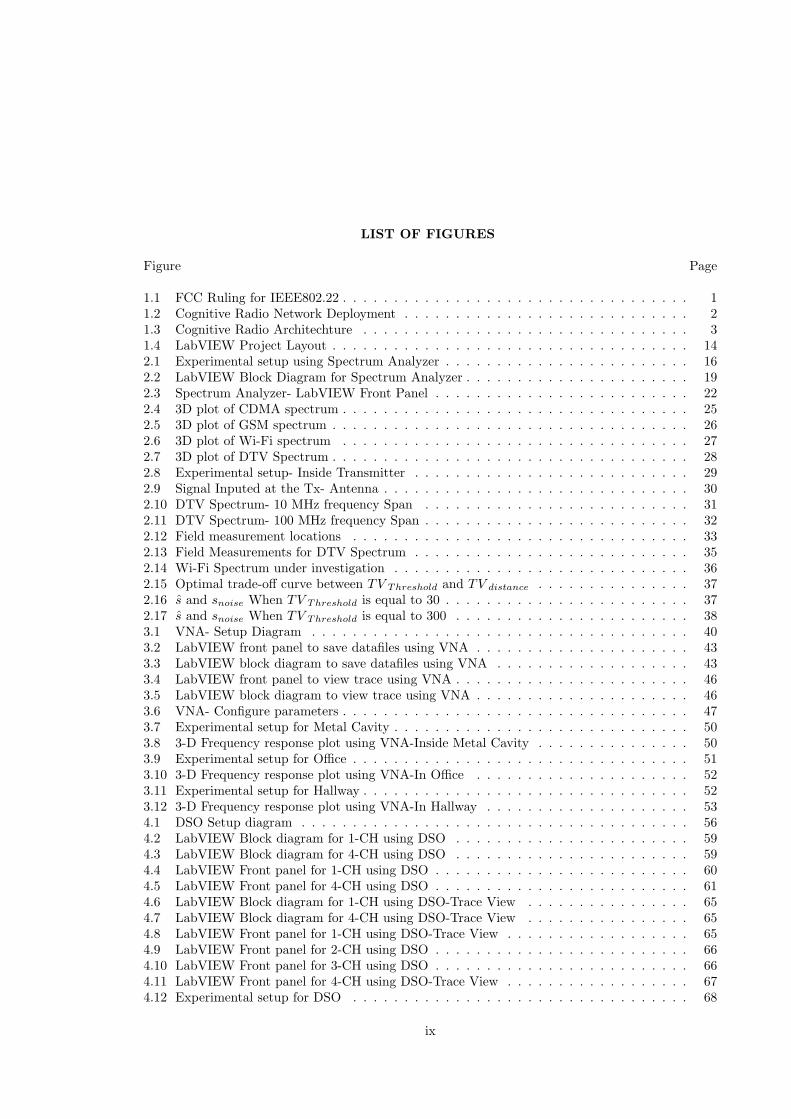
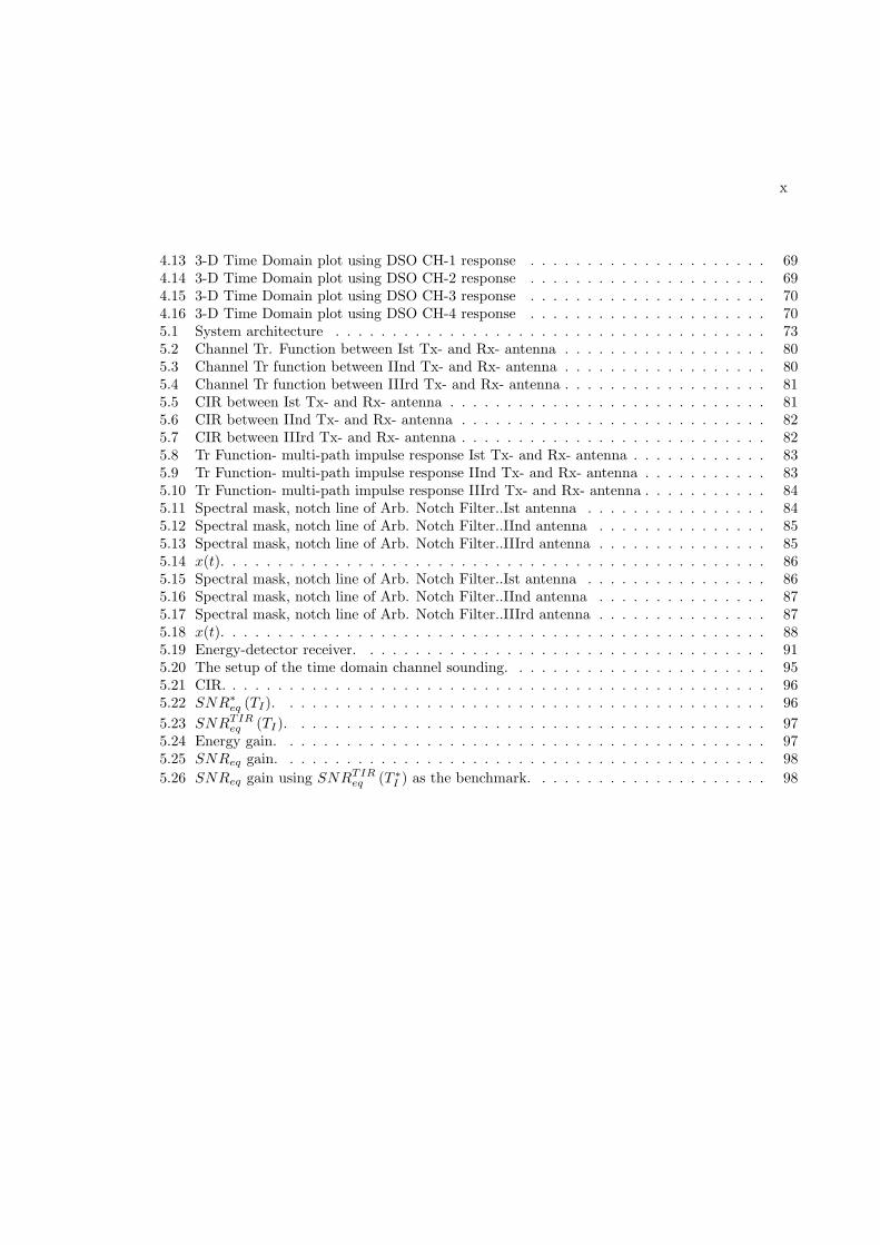
international standard [3]. Figure 1.1 shows the FCC’s ruling for IEEE802.22. Figure 1.2 shows the
IEEE802.22 network deployment.
Figure 1.1: FCC Ruling for IEEE802.22
1
2
Figure 1.2: Cognitive Radio Network Deployment
In particular, the spectrum scarcity is the most severe problem for US for wireless services,
partially due to the fact that US has most dense spectrum usage. There is a common belief that we
are running out of usable radio frequencies. Cognitive radio (CR) provides an alternative (a new
paradigm) to systems such as the third generation (3G) and the fourth generation (4G). Due to
the Department of Defense (DoD) focusing on the Joint Tactical Radio System (JTRS), US has a
clear technical leadership in cognitive radio. Cognitive radar [4], on the other hand, has the similar
demand for dynamic spectrum sharing. The advent of (multi-GHz) arbitrary waveform generators
has made it possible to change waveforms from pulse to pulse [5]. Until recently, sensor hardware
was not capable of changing the transmitted waveform in real time. But it is believed that the
sensor hardware can be leveraged by jointly considering wideband spectrum sensing and waveform
design. Anti-jamming, an example of electronic warfare, is critical and it is much harder to jam
3
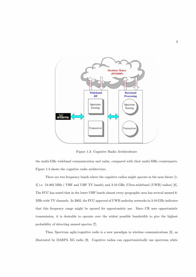
Figure 1.3: Cognitive Radio Architechture
the multi-GHz wideband communication and radar, compared with their multi-MHz counterparts.
Figure 1.3 shows the cognitive radio architecture.
There are two frequency bands where the cognitive radios might operate in the near future [1,
3] i.e. 54-862 MHz ( VHF and UHF TV bands) and 3-10 GHz (Ultra-wideband (UWB) radios) [6].
The FCC has noted that in the lower UHF bands almost every geographic area has several unused 6-
MHz wide TV channels. In 2002, the FCC approval of UWB underlay networks in 3-10 GHz indicates
that this frequency range might be opened for opportunistic use. Since CR uses opportunistic
transmission, it is desirable to operate over the widest possible bandwidth to give the highest
probability of detecting unused spectra [7].
Thus, Spectrum agile/cognitive radio is a new paradigm in wireless communications [8], as
illustrated by DARPA XG radio [9]. Cognitive radios can opportunistically use spectrum white
4
space and increase usage by ten times [10]. Author contributed in [11], by providing spectrum
related data to the group.
Quickest detection [12] is a research topic since 1931 . It can be employed in tasks such as
remote sensing [13, 14, 15], signal segmentation [16], environmental monitoring [17, 18], medical
diagnosis [19, 20, 21, 22, 23, 24, 25], and network security [26, 27, 28, 29, 30, 31]. In recent years,
decentralized quickest detection is also a topic wide open for studies [32, 33, 34]. References [35, 36]
shows a comprehensive introductions on quickest detection.
1.2 Channel Sounding
A channel is the propagation medium for a signal, which carries information from a trans-
mitter to a receiver. Rich multi-paths, with significant time resolution and very low power per
component is the key feature of Ultra-Wideband (UWB). By nature, a UWB channel is quasi-static,
thus the coherent time of the channel is very large. This is a relevant feature for the transmitter
to take full advantage of the channel state information (CSI) or CIR, and thus, perfect channel
estimation is realistic.
A pulse-based signal would be attenuated and distorted by propagation medium. Whereas, in
UWB, the short pulses follow multi-paths for propagation through the channel. When propagating
through the channel, the incident pulses acquire different shapes [37], as compared to the incident
pulse. Thus, if the channel transfer function is well-known, then a proper design of transmitter and
of UWB system. A UWB channel could be estimated by adapting two different approaches. The
first one is Frequency Domain (FD), channel sounding. In FD, a wide frequency band is swept by
a set of narrow band signals/pulses using a Vector network analyzer (VNA). The channel transfer
function, i.e. S-parameters of the respective channel, are thus recorded. Frequency shift, caused
by propagation delay due to long cables, and/or the large flight time [39], would induce possible
receiver will solve the problem [38]. Channel information is the key feature for the successful design
5
errors in channel sounding. An IFFT followed by Hermitian Processing [39] would be employed to
convert a frequency domain signal into the time domain. The second way for channel sounding is
Time Domain (TD)analysis. Channel impulse response could be obtained using this approach [39].
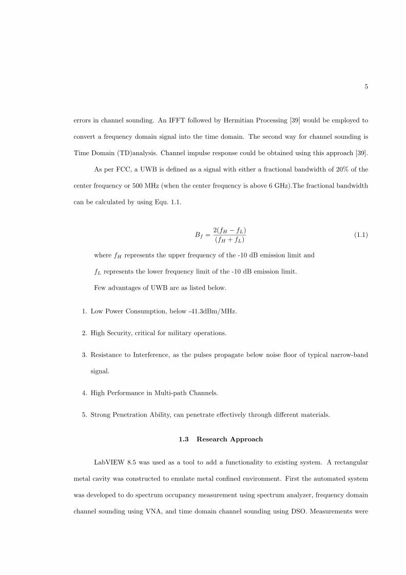
As per FCC, a UWB is defined as a signal with either a fractional bandwidth of 20% of the
center frequency or 500 MHz (when the center frequency is above 6 GHz).The fractional bandwidth
can be calculated by using Equ. 1.1.
Bf =2(fH − fL)
(fH + fL)(1.1)
where fH represents the upper frequency of the -10 dB emission limit and
fL represents the lower frequency limit of the -10 dB emission limit.
Few advantages of UWB are as listed below.
1. Low Power Consumption, below -41.3dBm/MHz.
2. High Security, critical for military operations.
3. Resistance to Interference, as the pulses propagate below noise floor of typical narrow-band
signal.
4. High Performance in Multi-path Channels.
5. Strong Penetration Ability, can penetrate effectively through different materials.
1.3 Research Approach
LabVIEW 8.5 was used as a tool to add a functionality to existing system. A rectangular
metal cavity was constructed to emulate metal confined environment. First the automated system
was developed to do spectrum occupancy measurement using spectrum analyzer, frequency domain
channel sounding using VNA, and time domain channel sounding using DSO. Measurements were
6
performed for the spectrums of CDMA, GSM, Wi-Fi, and DTV signals. Frequency domain channel
sounding in metal confined environment, office environment, and hallway environment were per-
formed. Time domain channel sounding for office environment was performed. The collected data
were used to for spectrum reconstruction. Waveform optimization for Multi input single output
(MISO) case was performed by using VNA data. Waveform optimization for Single input single
output (SISO) case was performed by using DSO data. Based on the spectrum occupancy measure-
ment using the current resources, it was concluded that the present resources for spectrum sensing
were limited. Thus, two new instruments viz. Arbitrary Waveform Generator(AWG) and Digital
Phosphor Oscilloscope (DPO) were recently purchased for better understanding of spectral behavior.
1.4 Introduction to LabVIEW
LabVIEW abbreviation of Laboratory Virtual Instrumentation Engineering Workbench is a
visual programming language from National Instruments. In 1986, it was originally released for
the Apple Macintosh and is commonly used for data acquisition, instrument control, and industrial
automation on a variety of platforms including Microsoft Windows, various versions of UNIX, Linux,
and Mac OS. The latest version of LabVIEW is version 8.6, released in August of 2008. LabVIEW
programs/subroutines are called virtual instruments (VIs). Each VI has three components:
1. Block Diagram: It is the main part where all the graphical programming is done; a block
diagram consists of VIs and even sub-VIs. Different VIs or sub-VIs are connected together
by using respective wire connections on the block diagram. Each wire connector has different
color, pertaining to the data type of the variable that is carried through the wire.
2. Front Panel: It is normally referred as the part where controls and indicators allow the operator
to input data into or extract data from a running VI. The required output/acquired data in
the form of graphs, data arrays, etc., are available on the the front panel.
7
3. Connector Panel: The connector pane is used to represent a VI in the block diagram of other
VIs.
The programming language used in LabVIEW is referred to as G and it is a dataflow pro-
gramming language, where the execution is determined by the structure of a graphical block diagram
(LV-source code) on which a programmer connects different functional nodes by drawing wires. The
wires propagate variables and any node can execute as soon as all its input data become available.
LabVIEW automatically ties the front panels into the development cycle.
LabVIEW 8.5 is used for test, control, and embedded system development. It is developed
and released by National Instruments (NI) and is the latest version of the graphical system design
platform. With the parallel dataflow language of LabVIEW, it is easy for users to map their
applications to multi-core and FPGA architectures for data streaming, control, analysis, and signal
processing. Based on the automatic multithreading capability of earlier versions, LabVIEW 8.5
scales user applications based on the total available number of cores and delivers enhanced thread-
safe drivers and libraries to improve throughput for RF, high-speed digital I/O, and mixed-signal test
applications. A new state-chart module’s inclusion in LabVIEW 8.5 helps engineers and scientists
to design and simulate event-based systems using familiar, high-level, Unified Modeling Language
(UML)-based standard state-chart notations. This new software also enables us to integrate more
advanced programmable automation controllers (PACs) with existing PLC-based industrial systems,
thus adding high-speed I/O and complex control logic to the industrial systems. Its new features
focus on predicting, detecting, and repairing cross-linking problems, including:
• The new Files View which shows your project contents in disk organization
• Tools for displaying and resolving multiple VIs of the same name referenced by a single project
8
• A new Find tool for the project, which help you find items by name and by caller/callee
relationship
• Auto-populating folders, which automatically update in response to content changes on disk.
LabVIEW includes extensive online and print documentation for new and experienced Lab-
VIEW users [40].
Several software toolkits such as signal processing and analysis tools, professional development
tools to optimize, test, and distribute Vis, third-party connectivity tools to Microsoft Office for
professional reporting, databases to access and store data and embedded design tools and control
and simulation tools are available to purchase for developing specialized applications in LabVIEW.
These toolkits integrate seamlessly in LabVIEW and after installing a LabVIEW add-on such as
a toolkit, module, or driver, the documentation for that add-on appears in the LabVIEW Help.
Following is a brief overview of these tool kits [41].
1. Signal Processing and Analysis
This toolbox includes the following basic signal processing and analysis toolkits.
• Digital Filter Design Toolkit: This toolkit extends the LabVIEW functionality and in-
teractive design stratigies to rapidly explore classical designs and to design, model, and
implement fixed-point and floating-point digital filters. Over 30 filter types, including
FIR, IIR, and multirate filters with well-known and special-purpose design options such
as Kaiser window, Dolph-Chebyshev, windowed, max flat, narrow-band (interpolated
FIR), elliptic, Chebyshev, Inverse Chebyshev, Butterworth, Bessel, notch/peak, max
flat, comb, halfband multirate, single-stage multirate, n-stage multirate, Nyquist multi-
rate, and root-raised/raised cosine multirate can be designed using this toolkit.
9
• Sound and Vibration Toolkit: This toolkit extends the LabVIEW functionality and out-
put indicators to handle audio measurements, fractional-octave analysis, swept sine anal-
ysis, sound-level measurements, frequency analysis, frequency response measurements,
transient analysis, and several sound and vibration displays such as waterfall displays.
Scaling, calibration, limit testing, weighting, and distortion and single-tone measurements
could be performed using this toolkit.
• Modulation Toolkit: This toolkit extends the built-in analysis capability of LabVIEW
with functionality and tools for signal generation, analysis, visualization, and processing of
standard and custom digital and analog modulation formats. A quality of measurements
including EVM and modulation error ratio (MER) could be provided using this toolkit;
it handles standard and custom modulation formats (AM, FM, PM, ASK, FSK, MSK,
GMSK, PSK, QPSK, PAM, QAM, CPM), simulates and measures impairments including
DC offset, IQ gain imbalance, and quadrature skew and offers bit-error rate (BER), phase
error, burst timing, and frequency deviation measurements.
• Spectral Measurements Toolkit: This toolkit extends the LabVIEW with functionality for
acquiring and analyzing spectral measurements and performing modulation and demod-
ulation on AM, FM, and PM signals. This toolkit includes 3D spectrogram capabilities,
power spectrum, peak power and frequency, in-band power, adjacent-channel power, and
occupied bandwidth.
2. Professional Development
This toolbox includes the following basic professional development toolkits to optimize, test,
and distribute VI’s.
• Real-Time Execution Trace Toolkit: This toolkit provides an interactive tool for analyzing
and verifying the execution of code with the LabVIEW Real-Time Module. We can
10
interactively analyze and benchmark thread and VI execution; optimize performance by
identifying memory allocation, sleep spans, and resource contention; and create execution
traces for LabVIEW Real-Time Module applications that you can print for documentation
and code reviews.
• Express VI Development Toolkit: This toolkit provides tools to help us create interactive
Express VIs such as to simplify the development of test, measurement, and control ap-
plications. Express VIs provide an interactive, configuration-based, easy-to-use interface
for end users.
• VI Analyzer Toolkit: This toolkit pinpoints improvements in the VI design, block diagram
code, documentation and VI properties and settings to optimize performance, usability,
and maintainability of the VIs.
3. Third-Party Connectivity Tools
This toolbox includes the following Third-Party connectivity toolkits such as to Microsoft
Office for professional reporting, databases to access, and store data and embedded design
tools
• Report Generation Toolkit for Microsoft Office: This toolkit provides a library of VI’s for
programmatically creating and editing Microsoft Word and Excel reports from LabVIEW.
• Database Connectivity Toolkit: This toolkit offers tools with which a quick connection
to local and remote databases can be made and perform common database operations
without having to perform structured query language (SQL) programming. By using
Microsoft ADO technology, this toolkit connects to the most popular databases such as
Microsoft Access, SQL Server, and Oracle databases.
11
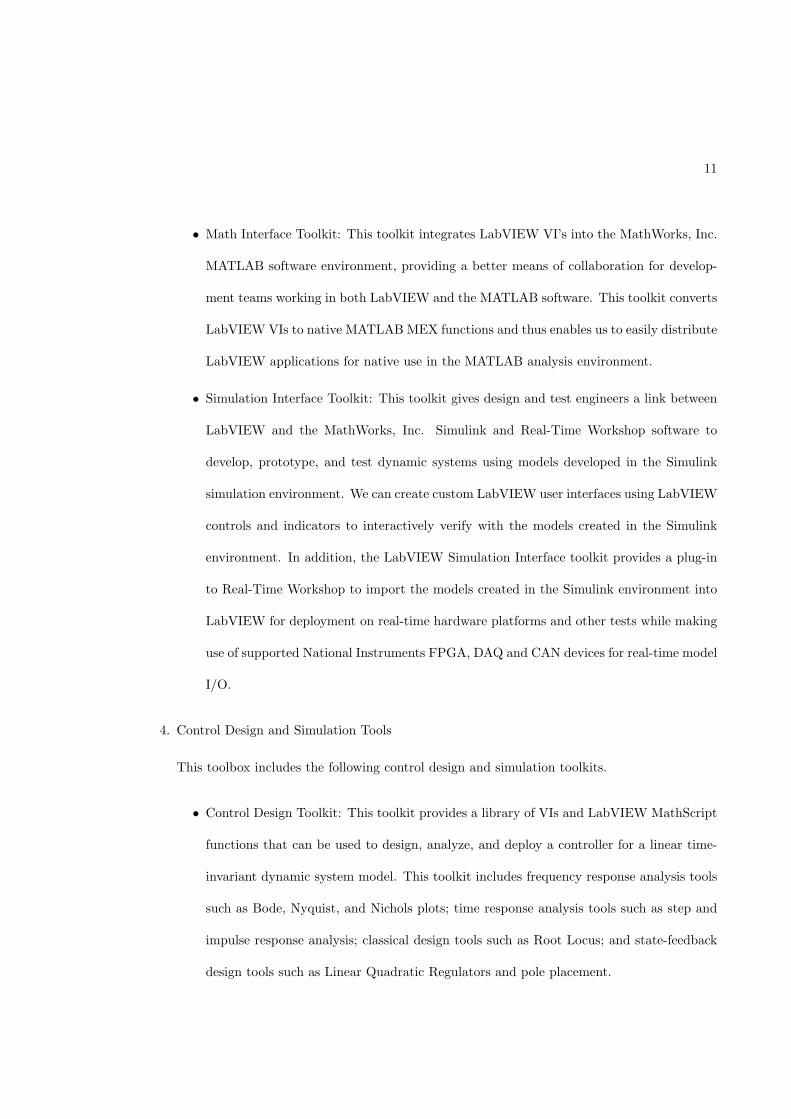
• Math Interface Toolkit: This toolkit integrates LabVIEW VI’s into the MathWorks, Inc.
MATLAB software environment, providing a better means of collaboration for develop-
ment teams working in both LabVIEW and the MATLAB software. This toolkit converts
LabVIEW VIs to native MATLAB MEX functions and thus enables us to easily distribute
LabVIEW applications for native use in the MATLAB analysis environment.
• Simulation Interface Toolkit: This toolkit gives design and test engineers a link between
LabVIEW and the MathWorks, Inc. Simulink and Real-Time Workshop software to
develop, prototype, and test dynamic systems using models developed in the Simulink
simulation environment. We can create custom LabVIEW user interfaces using LabVIEW
controls and indicators to interactively verify with the models created in the Simulink
environment. In addition, the LabVIEW Simulation Interface toolkit provides a plug-in
to Real-Time Workshop to import the models created in the Simulink environment into
LabVIEW for deployment on real-time hardware platforms and other tests while making
use of supported National Instruments FPGA, DAQ and CAN devices for real-time model
I/O.
4. Control Design and Simulation Tools
This toolbox includes the following control design and simulation toolkits.
• Control Design Toolkit: This toolkit provides a library of VIs and LabVIEW MathScript
functions that can be used to design, analyze, and deploy a controller for a linear time-
invariant dynamic system model. This toolkit includes frequency response analysis tools
such as Bode, Nyquist, and Nichols plots; time response analysis tools such as step and
impulse response analysis; classical design tools such as Root Locus; and state-feedback
design tools such as Linear Quadratic Regulators and pole placement.
12
In addition, this toolkit supports PID design, lead-lag compensators, predictive and con-
tinuous observers, and recursive Kalman filters for stochastic system models that incorpo-
rate measurement and process noise. This toolkit could also be used with the LabVIEW
Real-Time Module to deploy a discrete controller to a real-time target.
• PID Control Toolkit: This toolkit offers PID and fuzzy logic control functions that can
combine with the math and logic functions already in LabVIEW to graphically develop
control algorithms and programs for automated control.
• Simulation Module: This module provides VIs, functions, and other tools that can be
used to construct and simulate all or part of a dynamic system model. Both nonlinear
and linear dynamic system models are supported by this toolkit and it includes tools
for trimming and linearizing nonlinear models. The LabVIEW Simulation Module in-
cludes functions for describing continuous and discrete transfer function, zero-pole-gain
and state-space models as well as nonlinear phenomena such as friction, deadband, and
backlash.
One can interact with a model by using any of the VIs and functions included with
LabVIEW itself. One also can use the Simulation Module and the LabVIEW Real-Time
Module to deploy a continuous or discrete model to a real-time target.
• Statechart Module: This module assists in large-scale application development by pro-
viding a framework in which we can build, debug, and deploy statecharts in LabVIEW.
With the LabVIEW Statechart Module, we can create a statechart that reflects a com-
plex decision-making algorithm and then can generate the block diagram code necessary
to call the statechart from a VI.
The Statechart Module supports hierarchy, concurrency, and an event-based paradigm.
If we install the appropriate LabVIEW module, then we can execute statecharts on
13
supported real-time targets and National Instruments FPGA devices.
• System Identification Toolkit: This toolkit combines data acquisition tools with system
identification algorithms for accurate plant modeling. Useing LabVIEW System Identi-
fication toolkit with National Instruments hardware such as NI DAQ devices, to stimu-
late and acquire data from a plant and then to identify a dynamic system model. This
toolkit provides VI’s that support parametric, nonparametric, partially-known, and recur-
sive model estimation methods, AR, ARX, ARMAX, output-error, Box-Jenkins, transfer
function, zero-pole-gain, and state-space model forms, and Bode, Nyquist, and pole-zero
analysis. This toolkit also includes VIs for data preprocessing and model validation.
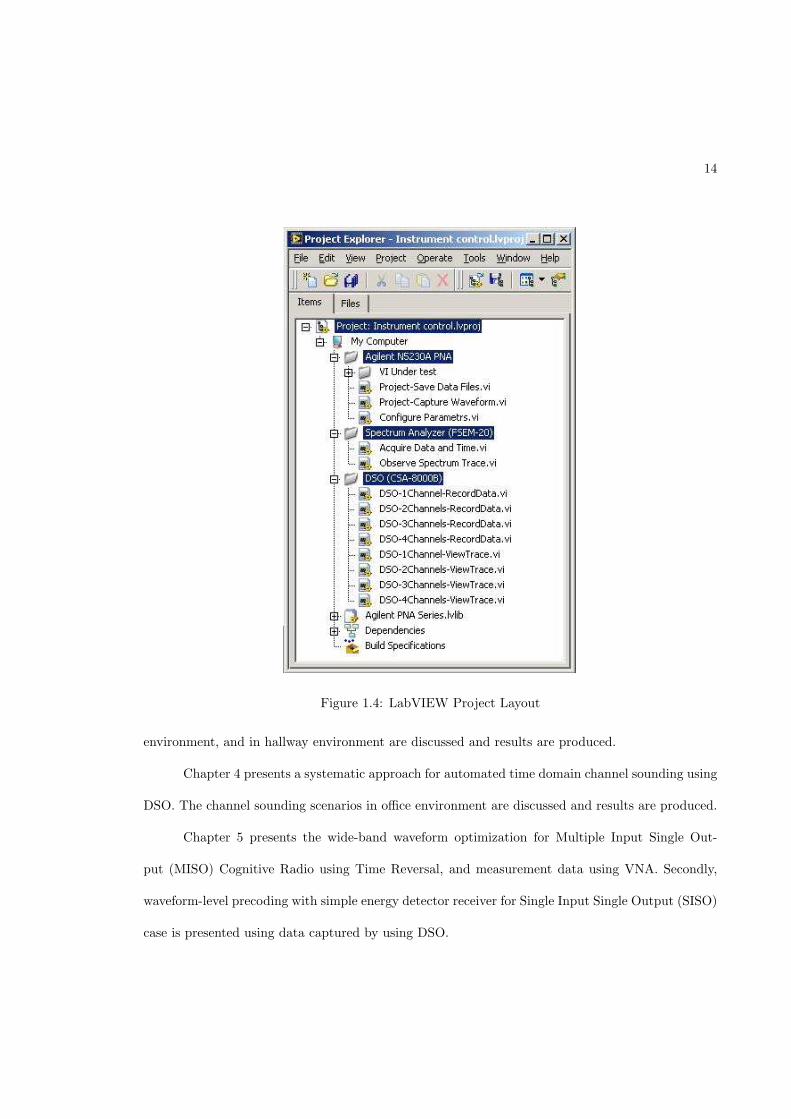
As LabVIEW is an industry standard for instrument control and data acquisition, the author
opted to use LabVIEW for controlling Rohde and Schwarz Spectrum analyzer, Agilent’s PNA-L
Vector network analyzer, and Tektronix CSA8000 Communication Signal Analyzer (DSO).
Figure 1.4 shows the LabVIEW project layout for the developed program.
As seen in Figure 1.4, the LabVIEW programs for all instruments are integrated in a single
project. Following is the detailed description of each instrument control VI.
1.5 Thesis Organization
Rest of the thesis is organized as follows:
Chapter 2 presents a systematic approach for automated spectrum occupancy measurement
using spectrum analyzer. Measurement/detection results are presented by using MatLab to process
the acquired spectrum data. An additional measurement results for the DTV signal strength are
discussed. Followed by spectrum reconstruction, using Total-Variation approach.
Chapter 3 presents a systematic approach for automated frequency domain channel sounding
using VNA. Three different channel sounding scenarios i.e. in metal confined environment, in office
14
Figure 1.4: LabVIEW Project Layout
environment, and in hallway environment are discussed and results are produced.
Chapter 4 presents a systematic approach for automated time domain channel sounding using
DSO. The channel sounding scenarios in office environment are discussed and results are produced.
Chapter 5 presents the wide-band waveform optimization for Multiple Input Single Out-
put (MISO) Cognitive Radio using Time Reversal, and measurement data using VNA. Secondly,
waveform-level precoding with simple energy detector receiver for Single Input Single Output (SISO)
case is presented using data captured by using DSO.
CHAPTER 2
SPECTRUM OCCUPANCY USING SPECTRUM ANALYZER
2.1 Introduction
A spectrum analyzer is used to display the power spectrum over a given frequency range.
The display changes as the properties of the signal change. There is a trade-off between frequency
resolution and how quickly the display can be updated. Frequency resolution can be defined as dis-
tinguishing frequency components that are close together. Here, spectrum analyzer is used to sense
the radio spectrum. Parameters, such as Start frequency, Stop frequency, Frequency span, Resolu-
tion bandwidth, Video bandwidth, etc., can be set on spectrum analyzer to see the corresponding
radio spectrum.
The goal of this work is to get the data corresponding to frequently changing radio spectrum,
for the future researches, such as for the modeling of the spectrum, the study on the efficient
algorithm of sensing spectrum and transmission schemes. To accomplish the goal of recording
quickly changing spectrum data, National Instruments (NI) LabVIEW 8.5 is used to control the
spectrum analyzer from a remote terminal.
Previously, spectrum analyzer was controlled manually and it was inefficient to save the
data of frequently changing spectrum by any means. Federal Communication System (FCC) in
its report [42, 43] mentioned that in order to develop future intelligent radio and to make the
opportunistic use [42, 44] of open white spaces [45, 46], the spectrum sensing must be performed
by the radio within a milliseconds level precision. Also, to develop a cognitive radio, some sort
of raw data pertaining to the power spectral density of a signal of a particular frequency band in
our immediate surroundings are the primary need of the wireless industry. Secondly, to develop
algorithms [47] for a more efficient and low cost intelligent radio, it is very important for the future
15
16
Computer / Laptop with LabVIEW- 8.5
Spectrum Analyzer
USB-GPIB connection
Rx Antenna
Maker : Rohde & Schwarz Model : FSEM-20 Freq. Range : 9kHz - 26.5GHz
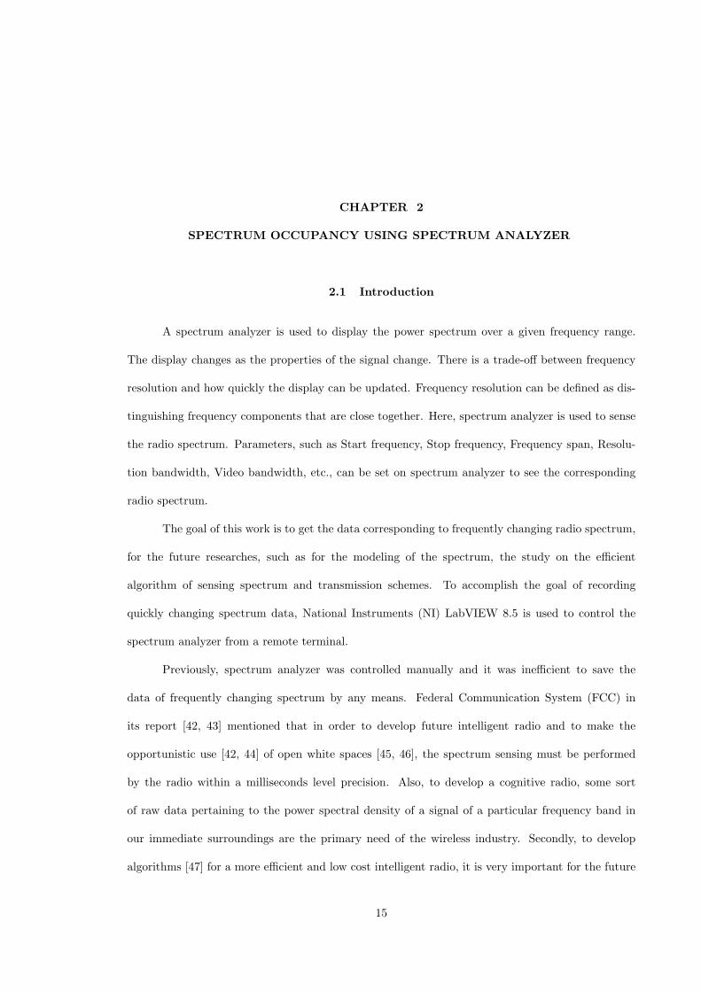
Figure 2.1: Experimental setup using Spectrum Analyzer
researchers to know the actual statistics of a radio spectrum. Hence, to address the problems of
quick sensing and collecting data over a long period of time, LabVIEW 8.5 is introduced to operate
spectrum analyzer remotely. In this way, the semi-continuous measurements over a long period of
time were performed and the data were collected automatically on the remote computer/laptop.
2.2 Instrument Setup
The sensing setup as seen in Figure 2.1 consists of a computer/laptop, a spectrum analyzer,
and one omni-directional antenna. NI LabVIEW 8.5 is installed on the computer/laptop to control
the spectrum analyzer and acquire the sensing data. The computer and spectrum analyzer are
connected using GPIB-USB2 cable. A linearly polarized omni-directional antenna with 50 ohm
unbalanced feed impedance is used for all sensing scenarios. As it is intended to receive and record
the data of the radio spectrum for digital television(DTV), CDMA, GSM, and Wi-Fi spectrum, thus
omni-directional antenna is the best choice to perform such sensing task.
17
2.3 Instrument Control using LabVIEW 8.5
The Spectrum analyzer under investigation is manufactured by Rohde and Schwarz, model
number FSEM20. This instrument has a capability to get the power spectrum of radio frequencies
ranging from 9kHz to 26.5GHz. However, the maximum numbers of data points per reading are fixed
to be 500. During remote control of spectrum analyzer, its operation via the front panel is disabled
and the analyzer remains in the remote state until it is reset to the manual state via the front panel
or via remote control interfaces. While switching from manual operation to remote control and vice
versa does not affect the remaining instrument settings. Before switchover from remote to manual
state, the already executing command processing must be completed as otherwise during switchover
the data could be lost or it may result into faulty data values.
Physically, the remote control mode is indicated by the LED “REMOTE” on the spectrum
analyzer’s front panel. In this mode the softkeys, the function fields, and the diagram labeling on
the analyzer’s display are not shown on the instruments screen. However, these settings could be
enabled by using “SYSTem:DISPlay:UPDate ON” command from remote terminal to check the
instrument settings. The RSIB or more commonly known as GPIB interface enables the instrument
to be controlled remotely by using LabVIEW or any other programming language/tools. When a
remote control is used, the analyzer’s GPIB port number is indicated on the remote terminal and
this number must be unique to all instruments if more than one instruments are subjected for remote
control.
The messages transferred via the data lines of the RSIB interface can be divided into two
groups, i.e.:
• Interface messages, where GPIB interface enables the instrument to be controlled by LabVIEW
or any other programming language/tools.
• Device messages, where the instrument is set to communicate to or from the remote terminal.
18
Standard Commands for Programmable Instruments (SCPI) were used to communicate with
analyzer through GPIB port of Analyzer. SCPI describes a standard command set for programming
instruments, irrespective of the type of instrument or manufacturer. The goal of the SCPI consor-
tium is to standardize the device-specific commands to a large extent. This is based on standard
IEEE 488.2. The detailed description of SCPI commands for the spectrum analyzer under inves-
tigation are listed in ”Chapter6:Remote Control-Description of Commands” of the corresponding
user manual [48, 49].
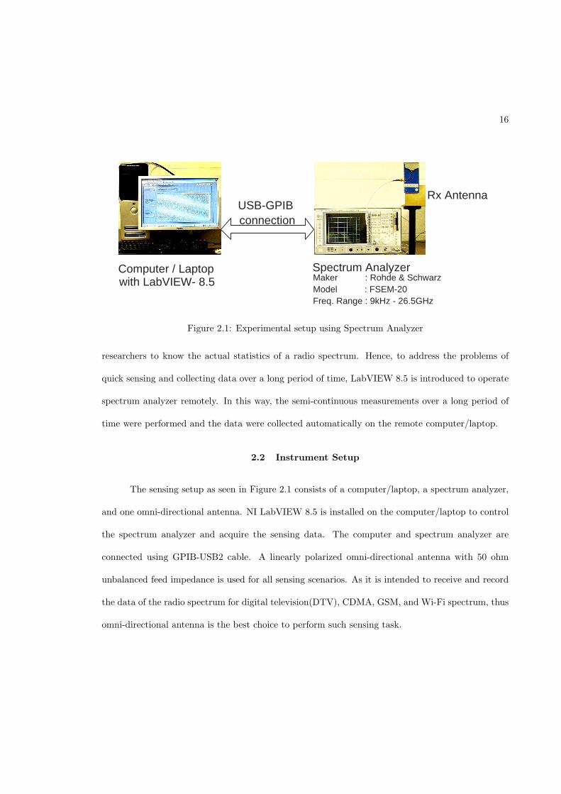
Figure 2.2 shows the block diagram of developed VI to control spectrum analyzer. The
LabVIEW-based instrument driver library for spectrum analyzer was available for download from
the Rohde and Schwarz website. These instrument driver VI’s were used as sub-VI’s in the developed
VI. All sub-VI’s were critically learned and investigated to better suit for the work under progress
ity(Detailed description is mentioned in the following steps) were wired together in such a manner
so as to efficiently achieve the desired goal at low cost. The real cost involved in this work was to
achieve the minimum duration of time interval between two set of measurement data. The outcome
of the developed work was to record each set of measurement data over a long time period. Mean-
while, the sensing time / time interval between two set of data, for each measurement, was recorded
in a different file. Here it is important to mention that one data set corresponds to 500 points of
the power spectral density of any signal acquired by using this spectrum analyzer and this number
is fixed by the manufacturer at the hardware level.
Following is the detailed procedural working of the developed VI for remote control of spec-
trum analyzer to record data and time over a long intervals.
1. Connect the spectrum analyzer, computer/laptop, and receiving antenna as shown in Fig-
ure 2.1.
and after careful investigation, different sub-VI’s along with other LabVIEW 8.5-based functional-
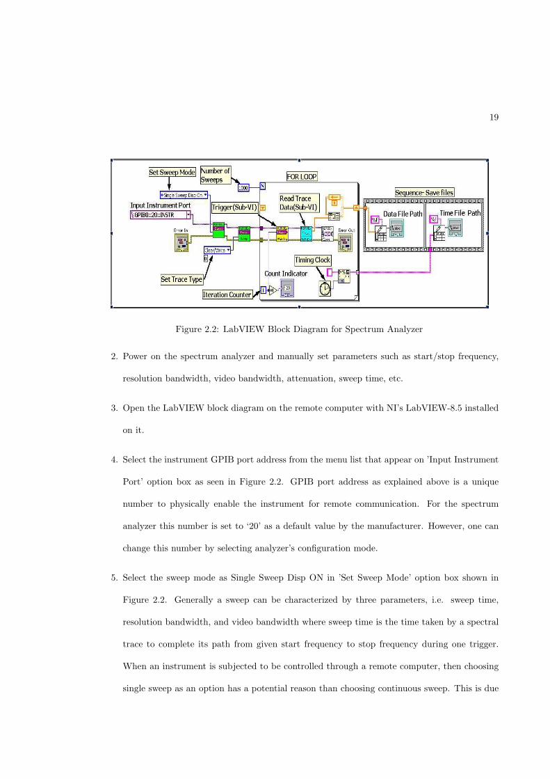
19
Figure 2.2: LabVIEW Block Diagram for Spectrum Analyzer
2. Power on the spectrum analyzer and manually set parameters such as start/stop frequency,
resolution bandwidth, video bandwidth, attenuation, sweep time, etc.
3. Open the LabVIEW block diagram on the remote computer with NI’s LabVIEW-8.5 installed
on it.
4. Select the instrument GPIB port address from the menu list that appear on ’Input Instrument
Port’ option box as seen in Figure 2.2. GPIB port address as explained above is a unique
number to physically enable the instrument for remote communication. For the spectrum
analyzer this number is set to ‘20’ as a default value by the manufacturer. However, one can
change this number by selecting analyzer’s configuration mode.
5. Select the sweep mode as Single Sweep Disp ON in ’Set Sweep Mode’ option box shown in
Figure 2.2. Generally a sweep can be characterized by three parameters, i.e. sweep time,
resolution bandwidth, and video bandwidth where sweep time is the time taken by a spectral
trace to complete its path from given start frequency to stop frequency during one trigger.
When an instrument is subjected to be controlled through a remote computer, then choosing
single sweep as an option has a potential reason than choosing continuous sweep. This is due
20
to fact that when data acquisition is done from a remote computer and if the sweep mode
is set as continuous sweep, then sensed data are not trustable. Using sweep type as single
sweep enables us to differentiate between each set of sensed data. But, in the later case, a
quick trigger is required to re-initiate the sweeping process for continuous sensing. This is only
possible if a automated triggering process could be included on the remote terminal to control
analyzer.
6. Select the appropriate trace mode in ’Set Trace Type’ option box shown in Figure 2.2. As
discussed earlier, a trace consists of 500 pixels on the horizontal frequency axis, that means
the number of point for each measurement is 500. Selection of trace mode depends on one’s
goal i.e. what type of data one needs from the spectrum analyzer. Generally for this spectrum
analyzer, commonly mentioned trace modes are:
• Clear/Write: In this mode, the trace memory is overwritten by each sweep, i.e. if this
mode is selected then the memory value of previous trace is cleared and we get new data
values during each sweep.
• Average: With this mode, an average is taken from several foregoing measurements.When
this mode is selected, then the first trace is recorded as discussed in Clear/Write mode and
from the second measurement onwards an average is formed on each succeeding sweeps.
• Max Hold: In this mode, the spectrum analyzer saves only the maximum values of
previous and current traces. In this way, the maximum value attained by the signal can
be determined over several sweeps.
• Min Hold: Unlike Max Hold, Min Hold represents only the minimum values of the pre-
vious and current traces. In this way, the minimum values attained by the signal can be
determined over several sweeps.
21
7. A ’FOR LOOP’ is introduced in the next step. This FOR LOOP serves as the main functioning
block to acquire the spectral data, time intervals between two different set of measurements,
and allow user to save the data file and timing file locally on remote computer’s hard disk.
Following are the steps describing the detailed functionality attached with this FOR LOOP.
• As seen in Figure 2.2, inside the ’FOR LOOP’ is a sub VI to trigger spectrum analyzer and
another sub-VI to read acquired trace data from the spectrum analyzer. These sub-VIs
are wired one after another and during each iteration of loop; first a trigger is sent to the
spectrum analyzer and then the sensing data are acquired pertaining to each iteration.
As it was pointed out in step 5, that a quick trigger is needed each time to re-initialize
a spectral trace to acquire signal value. Hence a triggering sub-VI is employed here to
accomplish the job.
Outside and at the top left corner of this loop is an option box ’Number of Sweeps’;
here user has to type a number. This number signifies that this FOR LOOP executes
repeatedly until the iteration counter ’i’, shown inside at left bottom of loop, achieves a
value equal to this typed number. For example as seen in Figure 2.2 this number is set
to 1000, which means we get the sensed spectrum data for 1000 sweeps.
• The second important functionality attached with this FOR LOOP is to acquire the
time taken to complete each iteration. A ’Timing Clock’ is placed inside the loop, as
seen in Figure 2.2. This clock automatically generates a millisecond timing value at
the start of each iteration. The millisecond time values are in synchronization with the
previous values during each FOR LOOP iteration and hence gives user a correct sequence
of numbers, which are further subjected for MatLAB processing to give us the correct
difference value corresponding to execution of each iteration. Here it is important to
mentioned that the millisecond timing clock generates a time stamp during the start of
22
Figure 2.3: Spectrum Analyzer- LabVIEW Front Panel
each iteration. Thus first millisecond time stamp includes: analyzer’s triggering time,
trace sweep time, acquire data time, and to save the acquired data time, and then the
same process is followed during each iteration of the FOR LOOP.
• Finally, the sensed data values and the generated timing values are virtually accumulated
in the LabVIEW’s memory. After the execution of FOR LOOP, two pop-up windows
open automatically one after the other on the remote computer terminal. These pop-up
windows prompts user to input the file name and allow user to save the acquired sensing
data and timing files at a preffered location on remote computer/laptop’s hard disk.
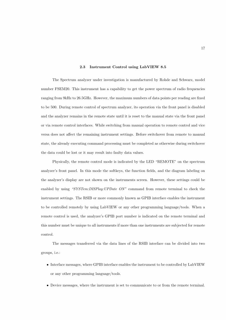
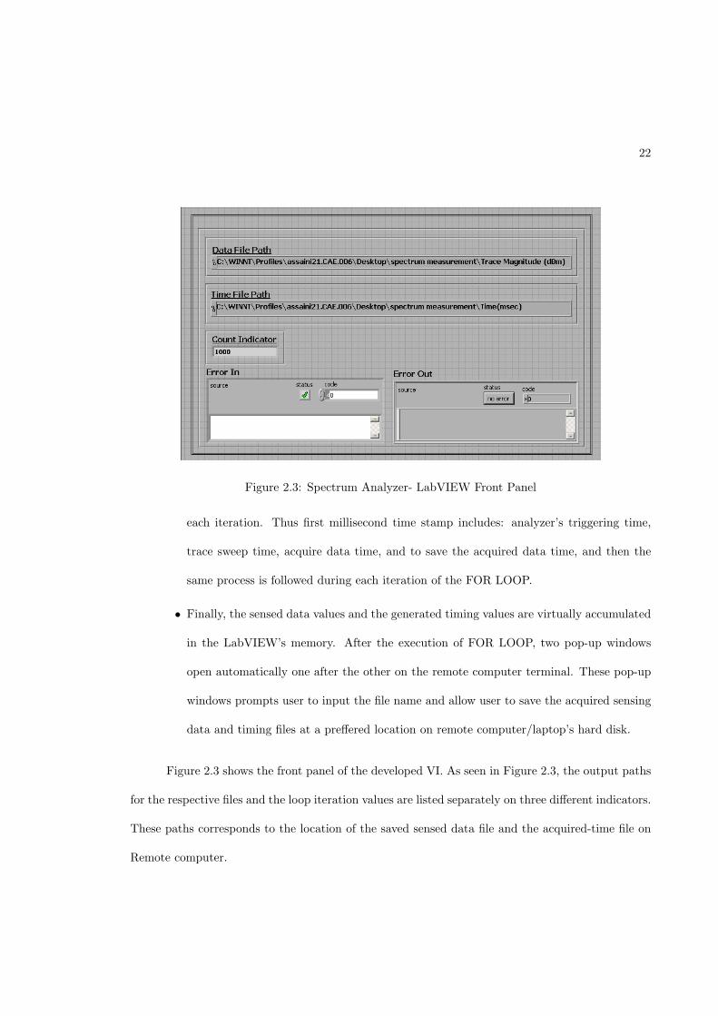
Figure 2.3 shows the front panel of the developed VI. As seen in Figure 2.3, the output paths
for the respective files and the loop iteration values are listed separately on three different indicators.
These paths corresponds to the location of the saved sensed data file and the acquired-time file on
Remote computer.
23
The saved files can easily be opened in notepad or word-pad in windows. These files can
directly be loaded in MatLAB for further data processing.
The data file contains row and columns of data values per iteration of the FOR LOOP. For
example if there are ‘N’ spectral traces to be measured then this data file is a matrix of ‘N X 500’,
where 500 is the number of columns and this number is fixed for each set of measurement. But since
there are only ‘N’ spectral traces to be measured, i.e. ‘N’ FOR LOOPS, so the acquired-time file
will show only one row of ‘N’ values, generated during start of each iteration LOOP.
2.4 Sensing Capability
The quick sensing is very important for cognitive radio to sense the real time and detailed
usage of the spectrum under any environment. The main advantage of this equipment-based spec-
trum sensing is that semi-continuous measurements can be executed and the corresponding sensed
data can be recorded automatically for the online or offline signal processing. The time delay be-
tween the continuous measurements is around 80-110ms, which includes the sweep time and time to
record/save data. In this way, more information about spectrum can be obtained and extracted. It
is again important to mention here that this is the fastest data available in the wireless industry as
of date.
2.5 Measurement Results
The scope of this work is to quickly sense the radio spectrum and this is done by adapting
a approach to control the spectrum analyzer from a remote terminal using LabVIEW 8.5 as a tool.
due to LabVIEW being an industry-wide standard, specifically developed for data acquisition and
control.
Four sensing scenarios were considered here.
The reason to use LabVIEW over any other softwares like C++, VisualC++, Simulink, etc., is
24
Table 2.1: Spectrum sensing parameters
Parameter ValueResolution Bandwidth 20kHz
Video Bandwidth 20kHzSweep Time 5 ms
RF Attenuation 10 dBTrace Type Clear/WriteSweep Mode Single Sweep Display ON
Number of Points 500 points per sweep
1. Spectrum sensing for CDMA signal.
2. Spectrum sensing for GSM signal.
3. Spectrum sensing for Wi-Fi signal.
4. A DTV signal is sensed from 697.5 MHz to 704.5MHz.
The first three spectrum sensings were executed in the indoor office environment and the
fourth for DTV signal was performed in the outdoor environment. The location of the indoor office
is at Wireless Networking Systems Lab and the outdoor location is the rooftop of Prescott Hall, both
of which are in Tennessee Technological University. Three-dimensional (3-D) spectrums of Time (s)
vs Frequency (MHz) vs Magnitude (dBm) were plotted using MATLAB for these four scenarios.
Spectrum measurements for one thousand sweeps were performed and one thousand sensing
data were recorded continuously in one spectrum sensing task. Each measurement consists of 500
data points. Thus, a total of 5,00,000 (1000*500) data points were acquired and recorded in each
spectrum sensing tast. Same parameters were used in all sensing scenarios. Table 2.1 shows the
parameter settings for each sensing scenario.
Following is the description of four scenarios as considered here.
25
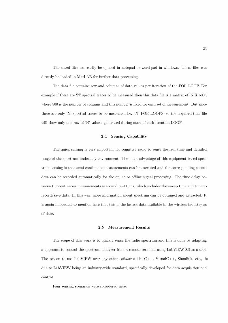
Figure 2.4: 3D plot of CDMA spectrum
2.5.1 Spectrum Sensing for CDMA Signal
the spectrum of CDMA signal was sensed. The sensed frequency band was from 800 MHz to 1100
MHz.
Figure 2.4 shows 3-D spectrum of CDMA signal. In Figure 2.4, the strong peaks between
800 MHz and 900 MHz show the CDMA signal, when a call connection is established between a
CDMA-based cell phone and a landline-based phone. Whereas, the blank spaces between these
strong peaks correspond to the time when call connection is not established.
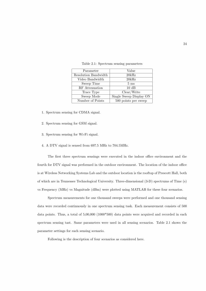
2.5.2 Spectrum Sensing for GSM Signal
spectrum of GSM signal was sensed. The sensed frequency band was from 1700 MHz to 2000 MHz.
Figure 2.5 shows 3-D spectrum of GSM signal. In Figure 2.5, strong peaks between 1850 MHz
and 1950 MHz show the GSM signal, when a call connection is established between a GSM-based
When a call connection was made from CDMA-based cell phone to landline based phone,
When a call connection was made from GSM-based cell phone to landline-based phone, the
26
Figure 2.5: 3D plot of GSM spectrum
correspond to the time when the call connection is not established.
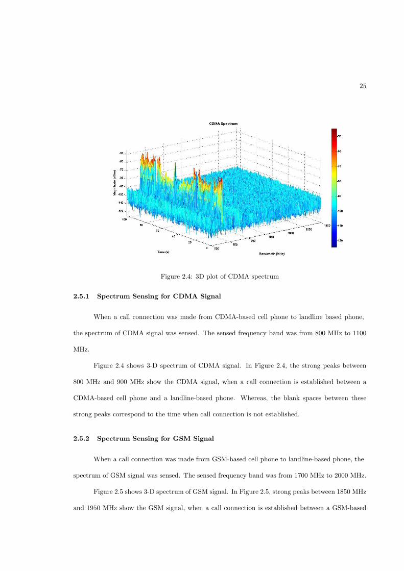
2.5.3 Spectrum Sensing for Wi-Fi Signal
When a Wi-Fi connection was established on notebook computer, the spectrum of Wi-Fi
signal was sensed. The sensed frequency band was from 2300 MHz to 2600 MHz.
Figure 2.6 shows 3-D spectrum of Wi-Fi signal. In Figure 2.6, strong peaks between 2400
MHz and 2500 MHz show the Wi-Fi signal, when a Wi-Fi connection is established on a Wi-Fi-
enabled notebook computer. A Wi-Fi signal is emitted by Wi-Fi-enabled router which is connected
with the CAT-5 cable provided by the University for Internet connection. Whereas, the blank spaces
between the strong peaks correspond to the time when the Wi-Fi connection is not established on
the notebook computer.
cell phone and a landline-based phone. Whereas, the blank spaces between these strong peaks
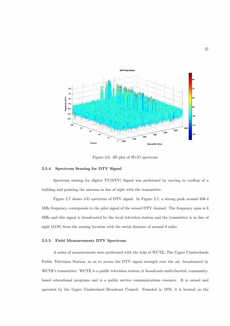
27
Figure 2.6: 3D plot of Wi-Fi spectrum
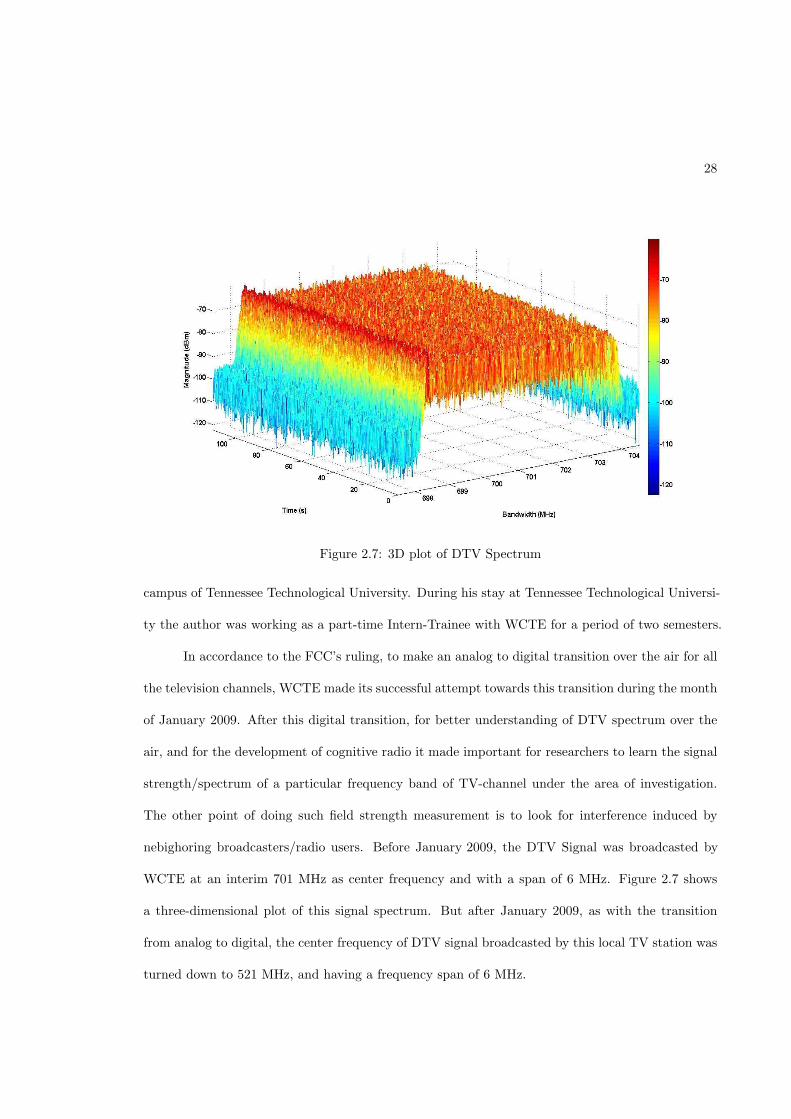
2.5.4 Spectrum Sensing for DTV Signal
Spectrum sensing for digital TV(DTV) Signal was performed by moving to rooftop of a
building and pointing the antenna in line of sight with the transmitter.
Figure 2.7 shows 3-D spectrum of DTV signal. In Figure 2.7, a strong peak around 698.4
MHz frequency corresponds to the pilot signal of the sensed DTV channel. The frequency span is 6
MHz and this signal is broadcasted by the local television station and the transmitter is in line of
sight (LOS) from the sensing location with the aerial distance of around 8 miles.
2.5.5 Field Measurements DTV Spectrum
A series of measurements were performed with the help of WCTE, The Upper Cumberlands
Public Television Station; so as to access the DTV signal strength over the air, broadcasted by
based educational programs and is a public service communications resource. It is owned and
operated by the Upper Cumberland Broadcast Council. Founded in 1978, it is located on the
WCTE’s transmitter. WCTE is a public television station; it broadcasts multi-faceted, community-
28
Figure 2.7: 3D plot of DTV Spectrum
In accordance to the FCC’s ruling, to make an analog to digital transition over the air for all
the television channels, WCTE made its successful attempt towards this transition during the month
of January 2009. After this digital transition, for better understanding of DTV spectrum over the
air, and for the development of cognitive radio it made important for researchers to learn the signal
strength/spectrum of a particular frequency band of TV-channel under the area of investigation.
The other point of doing such field strength measurement is to look for interference induced by
WCTE at an interim 701 MHz as center frequency and with a span of 6 MHz. Figure 2.7 shows
a three-dimensional plot of this signal spectrum. But after January 2009, as with the transition
from analog to digital, the center frequency of DTV signal broadcasted by this local TV station was
turned down to 521 MHz, and having a frequency span of 6 MHz.
campus of Tennessee Technological University. During his stay at Tennessee Technological Universi-
ty the author was working as a part-time Intern-Trainee with WCTE for a period of two semesters.
nebighoring broadcasters/radio users. Before January 2009, the DTV Signal was broadcasted by
29
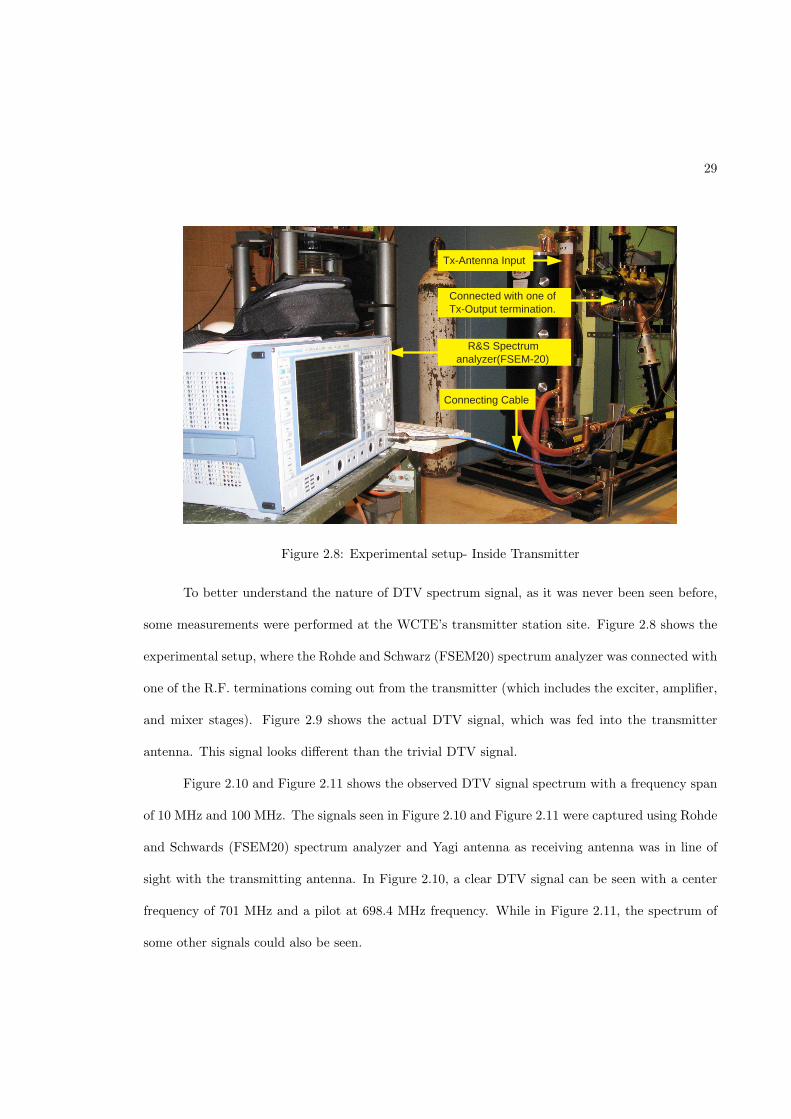
R&S Spectrum analyzer(FSEM-20)
Connecting Cable
Tx-Antenna Input
Connected with one of Tx-Output termination.
Figure 2.8: Experimental setup- Inside Transmitter
To better understand the nature of DTV spectrum signal, as it was never been seen before,
some measurements were performed at the WCTE’s transmitter station site. Figure 2.8 shows the
experimental setup, where the Rohde and Schwarz (FSEM20) spectrum analyzer was connected with
one of the R.F. terminations coming out from the transmitter (which includes the exciter, amplifier,
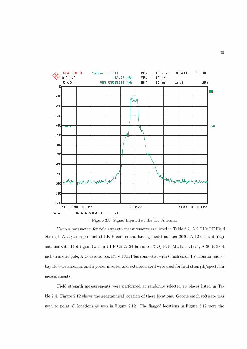
and mixer stages). Figure 2.9 shows the actual DTV signal, which was fed into the transmitter
antenna. This signal looks different than the trivial DTV signal.
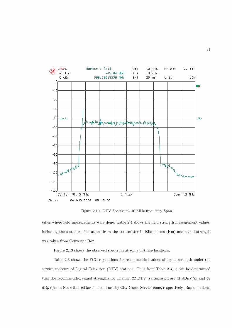
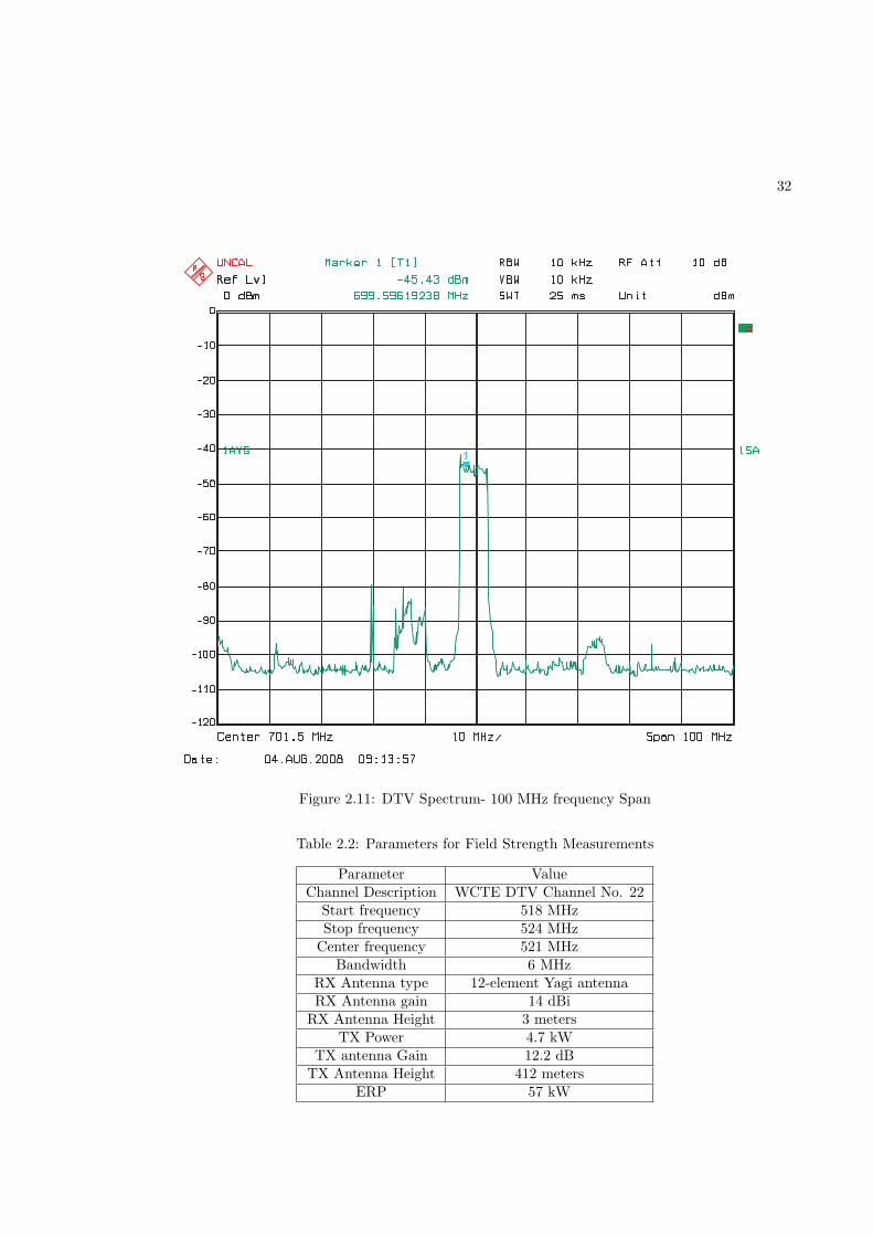
Figure 2.10 and Figure 2.11 shows the observed DTV signal spectrum with a frequency span
of 10 MHz and 100 MHz. The signals seen in Figure 2.10 and Figure 2.11 were captured using Rohde
and Schwards (FSEM20) spectrum analyzer and Yagi antenna as receiving antenna was in line of
sight with the transmitting antenna. In Figure 2.10, a clear DTV signal can be seen with a center
frequency of 701 MHz and a pilot at 698.4 MHz frequency. While in Figure 2.11, the spectrum of
some other signals could also be seen.
30
Figure 2.9: Signal Inputed at the Tx- Antenna
Strength Analyzer a product of BK Precision and having model number 2640, A 12 element Yagi
antenna with 14 dB gain (within UHF Ch.22-24 brand SITCO) P/N MU12-1-21/24, A 30 ft 3/ 4
inch diameter pole, A Converter box DTV PAL Plus connected with 6-inch color TV monitor and 8-
bay Bow-tie antenna, and a power inverter and extension cord were used for field strength/spectrum
measurements.
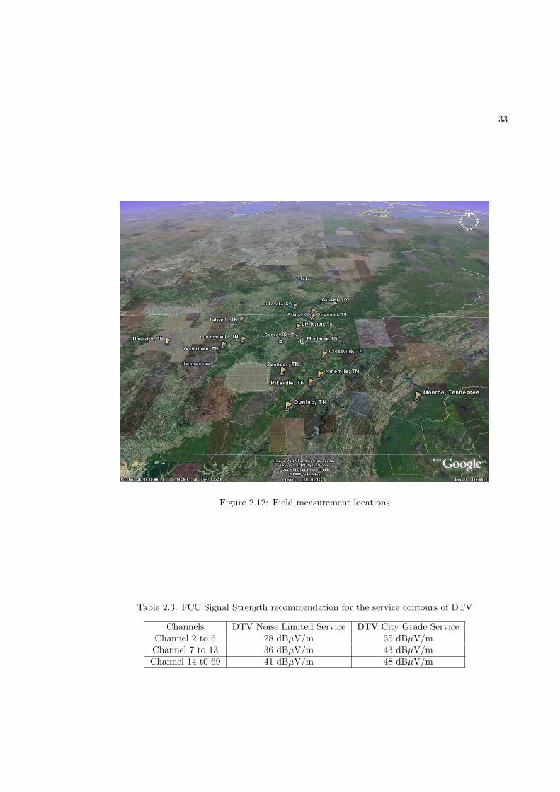
Field strength measurements were performed at randomly selected 15 places listed in Ta-
ble 2.4. Figure 2.12 shows the geographical location of these locations. Google earth software was
used to point all locations as seen in Figure 2.12. The flagged locations in Figure 2.12 were the
Various parameters for field strength measurements are listed in Table 2.2. A 2 GHz RF Field
31
Figure 2.10: DTV Spectrum- 10 MHz frequency Span
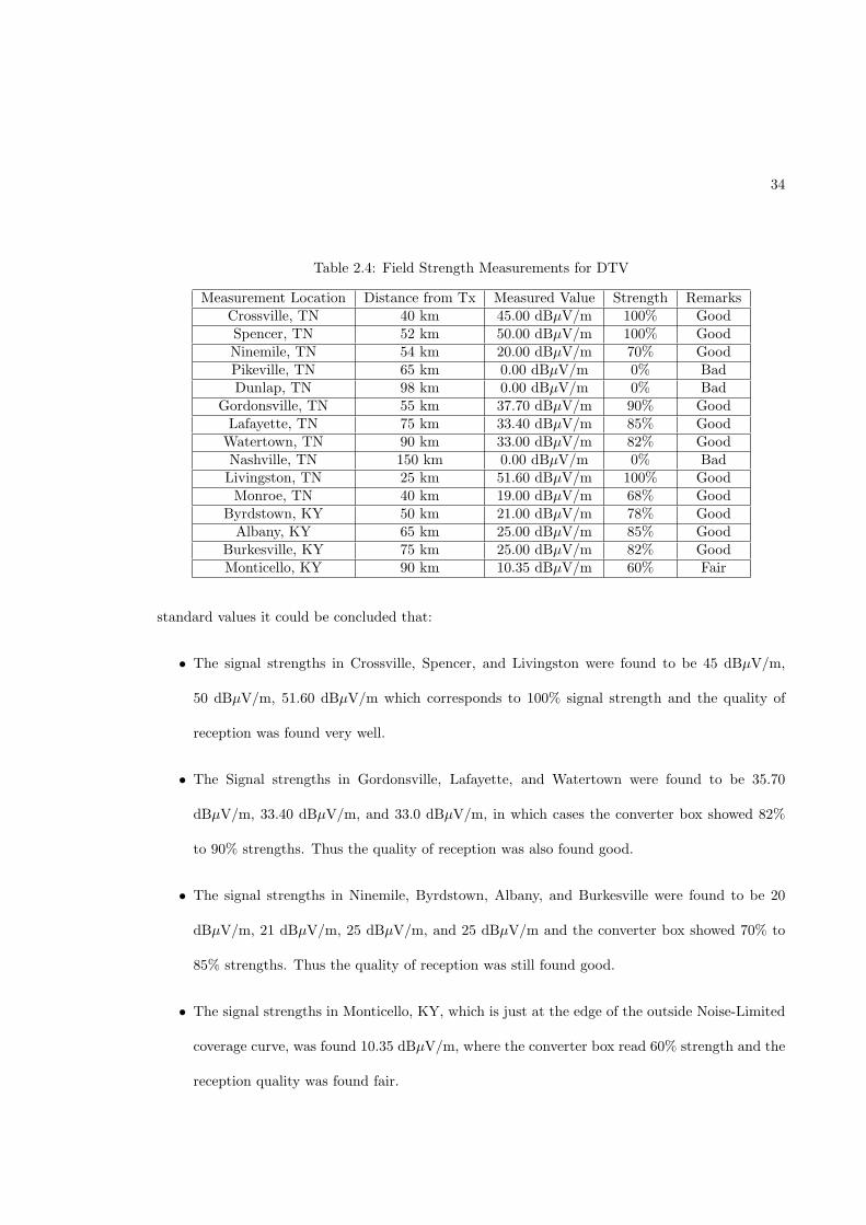
cities where field measurements were done. Table 2.4 shows the field strength measurement values,
including the distance of locations from the transmitter in Kilo-meters (Km) and signal strength
was taken from Converter Box.
Figure 2.13 shows the observed spectrum at some of these locations.
Table 2.3 shows the FCC regulations for recommended values of signal strength under the
service contours of Digital Television (DTV) stations. Thus from Table 2.3, it can be determined
that the recommended signal strengths for Channel 22 DTV transmission are 41 dBµV/m and 48
dBµV/m in Noise limited far zone and nearby City Grade Service zone, respectively. Based on these
32
Figure 2.11: DTV Spectrum- 100 MHz frequency Span
Table 2.2: Parameters for Field Strength Measurements
Parameter ValueChannel Description WCTE DTV Channel No. 22
Start frequency 518 MHzStop frequency 524 MHz
Center frequency 521 MHzBandwidth 6 MHz
RX Antenna type 12-element Yagi antennaRX Antenna gain 14 dBi
RX Antenna Height 3 metersTX Power 4.7 kW
TX antenna Gain 12.2 dBTX Antenna Height 412 meters
ERP 57 kW
33
Figure 2.12: Field measurement locations
Table 2.3: FCC Signal Strength recommendation for the service contours of DTV
Channels DTV Noise Limited Service DTV City Grade ServiceChannel 2 to 6 28 dBµV/m 35 dBµV/mChannel 7 to 13 36 dBµV/m 43 dBµV/mChannel 14 t0 69 41 dBµV/m 48 dBµV/m
34
Table 2.4: Field Strength Measurements for DTV
Measurement Location Distance from Tx Measured Value Strength RemarksCrossville, TN 40 km 45.00 dBµV/m 100% GoodSpencer, TN 52 km 50.00 dBµV/m 100% GoodNinemile, TN 54 km 20.00 dBµV/m 70% GoodPikeville, TN 65 km 0.00 dBµV/m 0% BadDunlap, TN 98 km 0.00 dBµV/m 0% Bad
Gordonsville, TN 55 km 37.70 dBµV/m 90% GoodLafayette, TN 75 km 33.40 dBµV/m 85% Good
Watertown, TN 90 km 33.00 dBµV/m 82% GoodNashville, TN 150 km 0.00 dBµV/m 0% BadLivingston, TN 25 km 51.60 dBµV/m 100% GoodMonroe, TN 40 km 19.00 dBµV/m 68% Good
Byrdstown, KY 50 km 21.00 dBµV/m 78% GoodAlbany, KY 65 km 25.00 dBµV/m 85% Good
Burkesville, KY 75 km 25.00 dBµV/m 82% GoodMonticello, KY 90 km 10.35 dBµV/m 60% Fair
standard values it could be concluded that:
• The signal strengths in Crossville, Spencer, and Livingston were found to be 45 dBµV/m,
50 dBµV/m, 51.60 dBµV/m which corresponds to 100% signal strength and the quality of
reception was found very well.
• The Signal strengths in Gordonsville, Lafayette, and Watertown were found to be 35.70
dBµV/m, 33.40 dBµV/m, and 33.0 dBµV/m, in which cases the converter box showed 82%
to 90% strengths. Thus the quality of reception was also found good.
• The signal strengths in Ninemile, Byrdstown, Albany, and Burkesville were found to be 20
dBµV/m, 21 dBµV/m, 25 dBµV/m, and 25 dBµV/m and the converter box showed 70% to
85% strengths. Thus the quality of reception was still found good.
• The signal strengths in Monticello, KY, which is just at the edge of the outside Noise-Limited
coverage curve, was found 10.35 dBµV/m, where the converter box read 60% strength and the
reception quality was found fair.
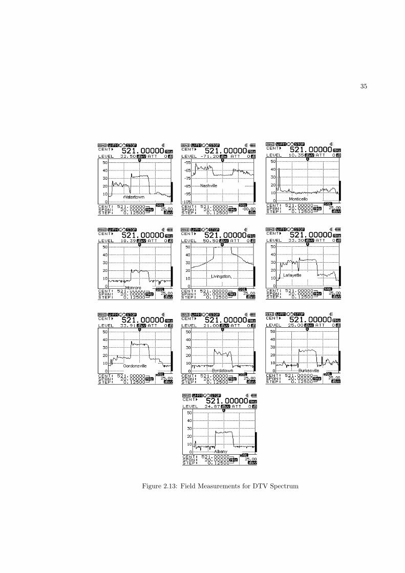
35
Figure 2.13: Field Measurements for DTV Spectrum
36
2300 2350 2400 2450 2500 2550 2600−120
−110
−100
−90
−80
−70
−60
−50Wi−Fi Spectrum
Bandwidth (MHz)
Mag
nitu
de (
dBm
)
Figure 2.14: Wi-Fi Spectrum under investigation
• However, no signal strengths and no reception were found in the Dunlap and Pikeville valley
areas (South zone). The reason for that was that both Dunlap and Pikeville stand at a very
low altitude and surrounded by a lot of by mountains and hills, which are most probably
blocking WCTE Channel 22 DTV signal.
2.6 Spectrum Reconstruction
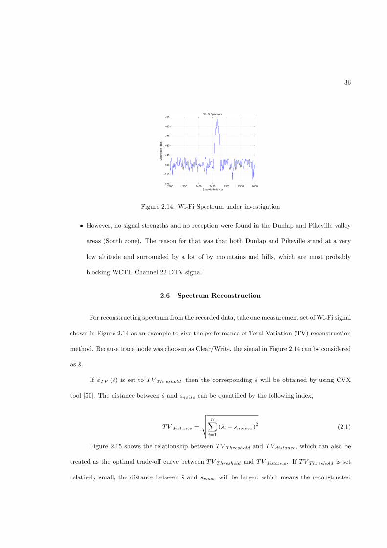
For reconstructing spectrum from the recorded data, take one measurement set of Wi-Fi signal
shown in Figure 2.14 as an example to give the performance of Total Variation (TV) reconstruction
method. Because trace mode was choosen as Clear/Write, the signal in Figure 2.14 can be considered
as s.
If φTV (s) is set to TV Threshold, then the corresponding s will be obtained by using CVX
tool [50]. The distance between s and snoise can be quantified by the following index,
TV distance =
√
√
√
√
n∑
i=1
(si − snoise,i)2
(2.1)
Figure 2.15 shows the relationship between TV Threshold and TV distance, which can also be
treated as the optimal trade-off curve between TV Threshold and TV distance. If TV Threshold is set
relatively small, the distance between s and snoise will be larger, which means the reconstructed
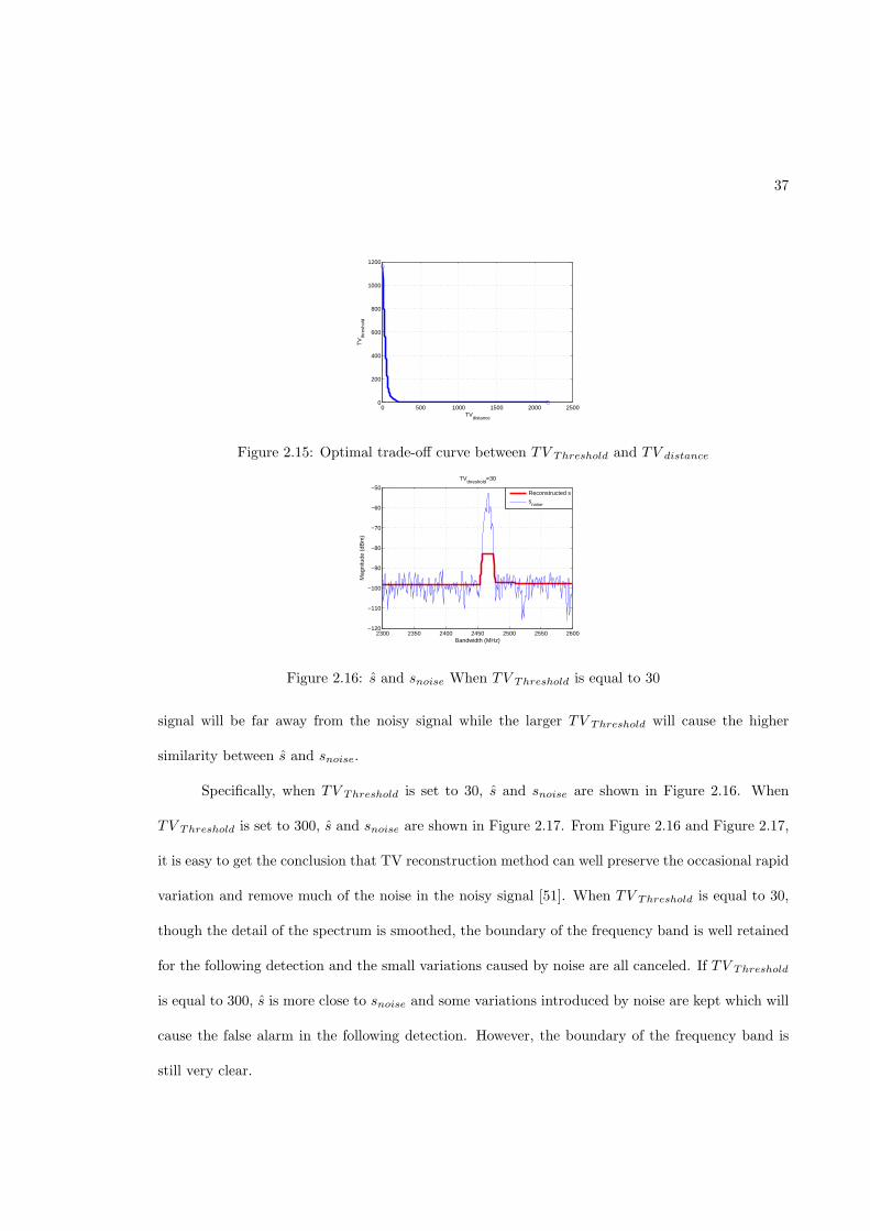
37
0 500 1000 1500 2000 25000
200
400
600
800
1000
1200
TVdistance
TV
thre
shol
d
Figure 2.15: Optimal trade-off curve between TV Threshold and TV distance
2300 2350 2400 2450 2500 2550 2600−120
−110
−100
−90
−80
−70
−60
−50
Bandwidth (MHz)
Mag
nitu
de (
dBm
)
TVthreshold
=30
Reconstructed ss
noise
Figure 2.16: s and snoise When TV Threshold is equal to 30
signal will be far away from the noisy signal while the larger TV Threshold will cause the higher
similarity between s and snoise.
Specifically, when TV Threshold is set to 30, s and snoise are shown in Figure 2.16. When
TV Threshold is set to 300, s and snoise are shown in Figure 2.17. From Figure 2.16 and Figure 2.17,
it is easy to get the conclusion that TV reconstruction method can well preserve the occasional rapid
variation and remove much of the noise in the noisy signal [51]. When TV Threshold is equal to 30,
though the detail of the spectrum is smoothed, the boundary of the frequency band is well retained
for the following detection and the small variations caused by noise are all canceled. If TV Threshold
is equal to 300, s is more close to snoise and some variations introduced by noise are kept which will
cause the false alarm in the following detection. However, the boundary of the frequency band is
still very clear.
38
2300 2350 2400 2450 2500 2550 2600−120
−110
−100
−90
−80
−70
−60
−50
Bandwidth (MHz)
Mag
nitu
de (
dBm
)
TVthreshold
=300
Reconstructed ss
noise
Figure 2.17: s and snoise When TV Threshold is equal to 300
2.6.1 Conclusion
If spectrum sensing is performed with high SNR, TV Threshold can be set higher to keep
more information about the spectrum while for the spectrum sensing with low SNR, TV Threshold
should be small to suppress the noise and preserve the boundary of the frequency band. Meanwhile,
TV reconstruction method can also be extended to rebuild the spectrums for the semi-continuous
measurements. For each measurement, TV reconstruction method with the same TV Threshold is
executed. Then, along the time axis, the change of the boundary of the frequency band will be
observed and detected, which will indirectly infer the availability of the frequency band of interest.
2.7 Summary
spectrum analyzer was discussed. The detailed functionality of the developed VI’s were discussed.
3-D plots of Frequency Vs Time Vs Power spectral density were shown for CDMA, GSM, Wi-Fi,
and DTV signal spectrum’s, using LabVIEW 8.5 to remotely control Spectrum analyzer, and finally
the discussion was extended to observe the behavior of DTV signal at the transmitting antenna
input and over the air at different locations, followed by an example to reconstruct spectrum from
the acquired data.
In this chapter, LabVIEW 8.5-based remote control for Rohde and Schwarzs (FSEM20),
CHAPTER 3
FREQUENCY DOMAIN CHANNEL SOUNDING USING VNA
3.1 Introduction
In wireless communication, our main concern is towards a signal with information content, so
that signal from a transmitter to receiver, with maximum efficiency and minimum distortion, could
be obtained. Thus, Vector network analysis of a signal is a method of accurately characterizing the
components of signal by measuring their effect on the amplitude and phase of swept-frequency and
swept-power. Generally, Vector Network Analyzers (VNA) are of two types:
1. Scalar Network Analyzer (SNA): Used to measures only amplitude properties of a signal.
2. Vector Network Analyzer (VNA): Used to measures both amplitude and phase properties of
a signal.
In VNA, the transmitter and receiver are co-located [52] so RF signal is generated as well
as received by VNA. Channel Sounding is carried out by sweeping a set of narrow-band sinusoid
signals through a wide frequency band. The VNA is operated in transfer function mode where one
of its ports serves as the transmitting port and the other as the receiving port. S-parameters are
used to express the complex frequency channel transfer function. Two-port VNA can measure four
individual S-parameters such as S11, S12, S21, and S22.
3.2 Instrument Setup
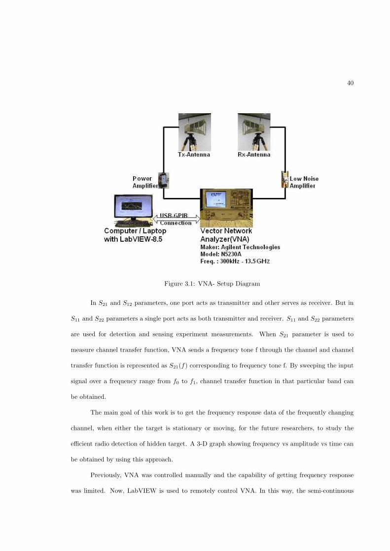
Figure 3.1 shows the experimental setup for VNA, when it is controlled from a remote terminal
using LabVIEW 8.5.
39
40
Figure 3.1: VNA- Setup Diagram
In S21 and S12 parameters, one port acts as transmitter and other serves as receiver. But in
S11 and S22 parameters a single port acts as both transmitter and receiver. S11 and S22 parameters
are used for detection and sensing experiment measurements. When S21 parameter is used to
measure channel transfer function, VNA sends a frequency tone f through the channel and channel
transfer function is represented as S21(f) corresponding to frequency tone f. By sweeping the input
signal over a frequency range from f0 to f1, channel transfer function in that particular band can
be obtained.
The main goal of this work is to get the frequency response data of the frequently changing
channel, when either the target is stationary or moving, for the future researchers, to study the
efficient radio detection of hidden target. A 3-D graph showing frequency vs amplitude vs time can
be obtained by using this approach.
Previously, VNA was controlled manually and the capability of getting frequency response
was limited. Now, LabVIEW is used to remotely control VNA. In this way, the semi-continuous
41
measurements can be done and the data can be recorded automatically in the form of CITI formated
files, on the VNA’s hard disk.
The time needed for each measurement is around 3s, which includes the sweep time and time
to record/save data files. In this way, more information about channel sounding can be obtained
and extracted. Figure 1.4 shows the LabVIEW project layout.
3.3 Instrument Control using LabVIEW 8.5
Depending on the need, this project is divided into two categories.
1. By recalling an already saved calibration file (.cst format) from the Instruments Hard disk.
2. Setting the network analyzer’s parameters using LabVIEW 8.5 from a remote terminal com-
puter.
Where in the earlier case it was assumed that first the instrument was calibrated manually
and the calibration state was saved at a particular location in PNA’s hard disk. Then the saved
calibration state was recalled using LabVIEW 8.5 from remote computer to perform measurements.
A calibration state consists of all parameters like Start frequency, Stop frequency, Power level,
Number of points, Sweep type, Sweep time, Average, and Trigger values. While the later case, VNA
parameters such as Start frequency, Stop frequency, Power level, Number of points, Sweep type,
Sweep time, etc., could be set from a remote terminal computer using LabVIEW 8.5 itself. This
way different parameters could be communicated by a remote connection to VNA.
The detailed description for both of these categories will be explained in the following sections.
3.3.1 By Recalling Calibration File
As mentioned before, it is assumed that the VNA is calibrated manually using specific cali-
bration kit provided by Agilent Technologies, in a particular environment to eliminate the induced
42
Table 3.1: VNA Parameters for Test Case
Parameter ValueStart Frequency 3GHzStop Frequency 4GHz
Power Level 0 dBmAverage Off
Number of points per sweep 1001Sweep Type Linear frequency
Trigger Single
resonance. Depending on the need, this category was further subdivided into two subcategories.
1. To save data files and timing file.
2. To capture waveform on remote terminal.
Here first one was used to record the data file (CITI formated) and save a timing file for each
set of measurement using LabVIEW 8.5 and the second one is just used to display the acquired
waveforms / frequency response of channel on LabVIEW front panel. The detailed description for
these subcategories is as explained below.
3.3.1.1 To save data files and timing file. Following steps describe the working for
saving the data files (CITI format) and timing file using LabVIEW 8.5 VI.
1. Manually set all the required parameters shown in Table 3.1 on VNA and calibrate the instru-
ment manually by using a standard calibration kit provided by Agilent Technologies. Calibra-
tion kit used to do calibration for VNA under investigation has a Model number of 8052, and
this kit has got the mechanical standards for calibration. Since the VNA under investigation
has a 2-port’s, so the mechanical standards used to calibrate this VNA were Open, Short,
Broadband load, and Through. Different standards used to calibrate.
Table 3.1 shows the approximate numbers assumed for this case only it is understood that
different number could be set, as per need, requirement and capability of instrument.
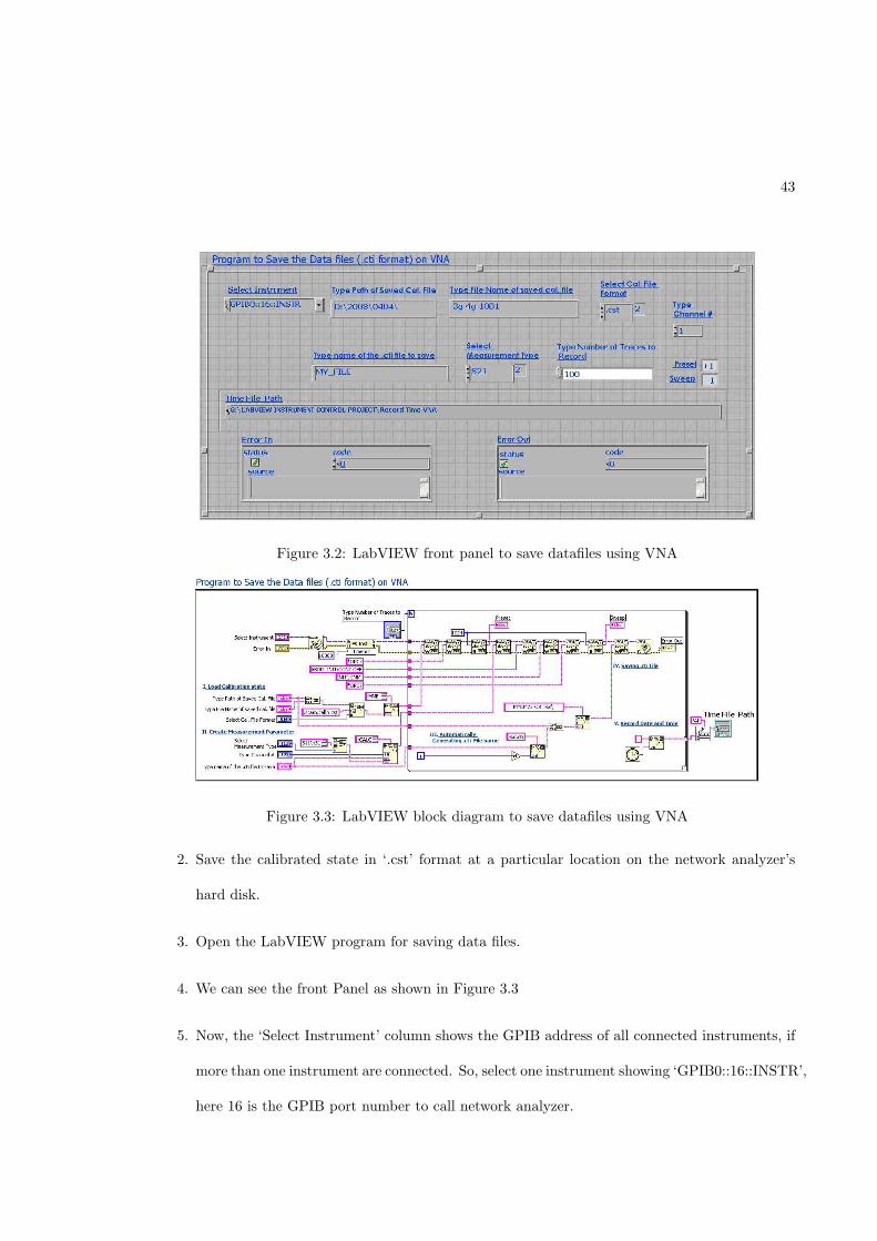
43
Figure 3.2: LabVIEW front panel to save datafiles using VNA
Figure 3.3: LabVIEW block diagram to save datafiles using VNA
2. Save the calibrated state in ‘.cst’ format at a particular location on the network analyzer’s
hard disk.
3. Open the LabVIEW program for saving data files.
4. We can see the front Panel as shown in Figure 3.3
5. Now, the ‘Select Instrument’ column shows the GPIB address of all connected instruments, if
more than one instrument are connected. So, select one instrument showing ‘GPIB0::16::INSTR’,
here 16 is the GPIB port number to call network analyzer.
44
6. Now type the Path, Filename, and File format in following three boxes, of the saved calibration
file. For example, in this case a calibration file named ‘3g-4g-1001.cst’ is stored at ‘D :
\2008\0404\’ path on network analyzer. So ‘D : \2008\0404\’ is typed in the File path, ‘3g-
4g-1001’ is typed in the file name field and file format ‘.cst’ is selected from the drop-down
menu, respectively, as shown in Figure 3.3.
File format type column consists of three options to select, i.e.
• ‘.sta’ format, represented by option number 0.
• ‘.cal’ format, represented by option number 1.
• ‘.cst’ format, represented by option number 2.
The option number i.e. 0, 1, and 2 can be seen in the next little box.
7. Now the file name, ‘MY-FILE’ in this case, can be typed in the next field named ‘Type name
of the .cti file to save’. As it is required to save many data files automatically using LabVIEW,
thus the program is coded in such a manner that it will generate and start append numeric
numbers (in ascending order) to the given filename string which will not only significantly
reduce time to save each file but also prohibit the duplication of files names.
8. Now, the measurement type, i.e. S11, S12, S21, S22 can be selected from the drop-down menu
and the next box shows option numbers for measurement type, as shown in Figure 3.3 where
• 0 implies ‘S11’
• 1 implies ‘S12’
• 2 implies ‘S21’
• 3 implies ‘S22’
45
9. Type the number of traces to record as data files (.cti formated), in the field ‘Type number of
traces to Record’. After execution, program stops automatically when this number is achieved.
As seen in Figure 3.3 this number is 100, means for this particular case, when the program is
executed then 100 number of ‘.cti’ files were generated an saved on VNA’s hard disk.
After completion of program, data files can be copied to flash drive from VNA’s hard disk
and further Matlab based analysis on acquired data could be performed.
Two flags, ‘Preset’ and ‘Sweep’, are included to check the program flow. Flag value ‘+1’
means program is running ok and ‘0’ means there is an error before the flag value is achieved. Also,
if there is an error then error number and its description are shown in error out box.
3.3.1.2 To capture waveform on remote terminal. The other functionality is to
capture the waveform from network analyzer. Figure 3.5 shows the labVIEW front panel of captured
waveform. This program also follows exactly same Steps[1-10] as discussed above. But here our
purpose is to observe the waveforms on remote terminal, as they can be seen on network analyzer’s
screen. So, instead of generating any filename, a graphic display is added in this VI, which enables
us to see the captured waveform.
The X-axis in waveform graph corresponds to frequency in Hz and Y-Axis corresponds to
magnitude power in dbm. Both scales are set to auto adjusting mode, so that for different values
of start/stop frequency, graphical display of waveform can adjust by itself. For example, in present
case, Start frequency is 3GHz and Stop frequency is 4GHz, so the X-axis scale shows frequency
range starting from 3GHz to 4 GHz as seen in Figure 3.5. The acquired trace can be copied from
the LabVIEW front panel and then can save as in JPG format.
3.3.2 Setting the Network Analyzer’s Parameters using LabVIEW 8.5
1. To configure VNA parameters from remote terminal computer.
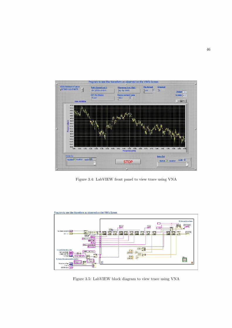
46
Figure 3.4: LabVIEW front panel to view trace using VNA
Figure 3.5: LabVIEW block diagram to view trace using VNA
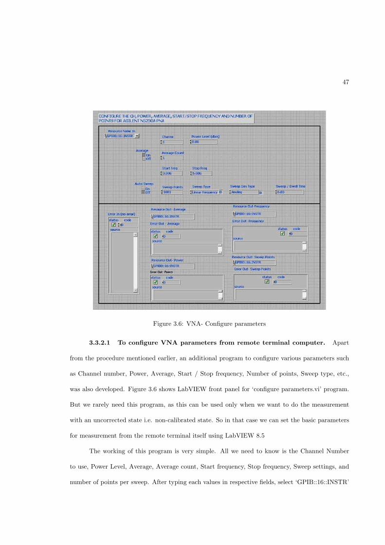
47
Figure 3.6: VNA- Configure parameters
3.3.2.1 To configure VNA parameters from remote terminal computer. Apart
from the procedure mentioned earlier, an additional program to configure various parameters such
as Channel number, Power, Average, Start / Stop frequency, Number of points, Sweep type, etc.,
was also developed. Figure 3.6 shows LabVIEW front panel for ‘configure parameters.vi’ program.
But we rarely need this program, as this can be used only when we want to do the measurement
with an uncorrected state i.e. non-calibrated state. So in that case we can set the basic parameters
for measurement from the remote terminal itself using LabVIEW 8.5
The working of this program is very simple. All we need to know is the Channel Number
to use, Power Level, Average, Average count, Start frequency, Stop frequency, Sweep settings, and
number of points per sweep. After typing each values in respective fields, select ‘GPIB::16::INSTR’
48
in the ‘Resource Name In’ column and run the program once. We can observe the new settings on
the network analyzer’s screen.
3.4 Measurement Results
Measurements using VNA were performed and LabVIEW being used to control VNA from a
remote laptop. The purpose for performing these measurements were to show the acquired capability
to do automated and semi-continuous measurements over long time periods. In this way more data
were recorded in less time.
Three different scenarios were considered to perform such measurements, as listed below.
1. Inside rectangular metal cavity.
2. In the office environment.
3. In the hallway.
The experimental parameters are listed in Table 3.2 and same parameters were used for all
three measurement scenarios. The VNA was calibrated using the parameters listed in Table 3.2.
The calibration state was saved as a “.cst” formated file in VNA’s hard disk. This calibration file
Figure 3.7.
Figure 3.7 shows the experimental setup for first scenario measurements i.e. inside rectangular
metal cavity. The metal cavity was built in the room number CH-403 of Clement hall located at
Tennessee Technological University(TTU). The metal cavity was 15.11 by 7.83 by 7.66 feet. The
transmitter (Tx) and receiver (Rx) antenna were put inside the metal cavity. Tx and Rx were placed
3 meters apart from each other, in the center of metal cavity. Tx and Rx- antenna height was 3.94
feet. Two uni-directional HORN Antennas, with frequency range 700 MHz to 13 GHz were used
was recalled from LabVIEW-based remote terminal, which was a laptop in this case as shown in
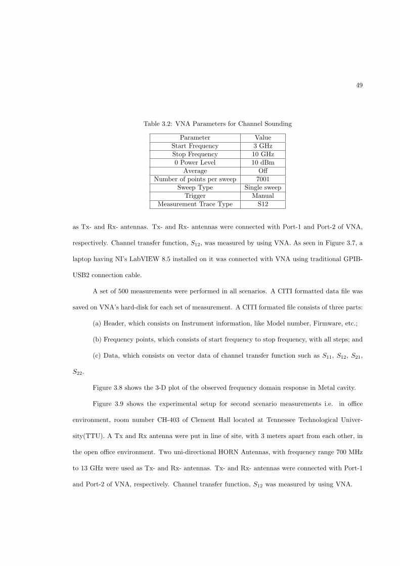
49
Table 3.2: VNA Parameters for Channel Sounding
Parameter ValueStart Frequency 3 GHzStop Frequency 10 GHz0 Power Level 10 dBm
Average OffNumber of points per sweep 7001
Sweep Type Single sweepTrigger Manual
Measurement Trace Type S12
as Tx- and Rx- antennas. Tx- and Rx- antennas were connected with Port-1 and Port-2 of VNA,
respectively. Channel transfer function, S12, was measured by using VNA. As seen in Figure 3.7, a
laptop having NI’s LabVIEW 8.5 installed on it was connected with VNA using traditional GPIB-
USB2 connection cable.
A set of 500 measurements were performed in all scenarios. A CITI formatted data file was
saved on VNA’s hard-disk for each set of measurement. A CITI formated file consists of three parts:
(a) Header, which consists on Instrument information, like Model number, Firmware, etc.;
(b) Frequency points, which consists of start frequency to stop frequency, with all steps; and
(c) Data, which consists on vector data of channel transfer function such as S11, S12, S21,
S22.
Figure 3.8 shows the 3-D plot of the observed frequency domain response in Metal cavity.
Figure 3.9 shows the experimental setup for second scenario measurements i.e. in office
environment, room number CH-403 of Clement Hall located at Tennessee Technological Univer-
sity(TTU). A Tx and Rx antenna were put in line of site, with 3 meters apart from each other, in
the open office environment. Two uni-directional HORN Antennas, with frequency range 700 MHz
to 13 GHz were used as Tx- and Rx- antennas. Tx- and Rx- antennas were connected with Port-1
12and Port-2 of VNA, respectively. Channel transfer function, S was measured by using VNA.
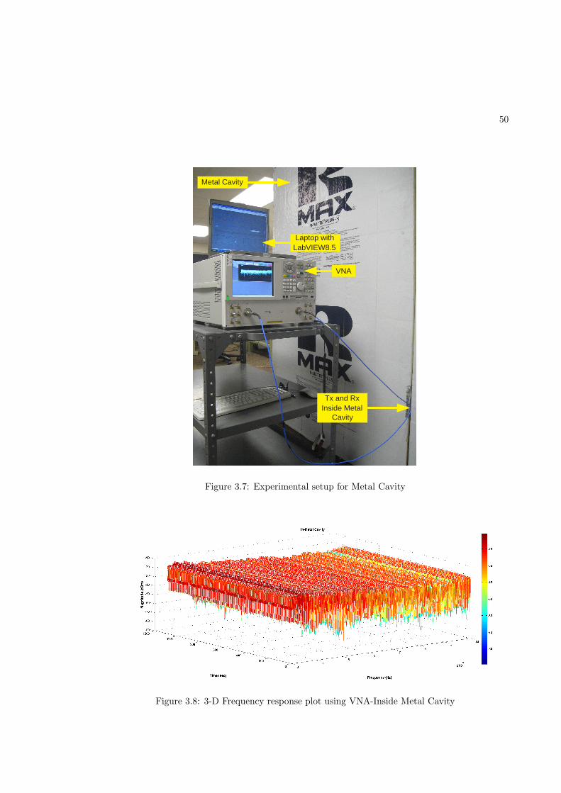
50
Laptop with LabVIEW8.5
VNA
Metal Cavity
Tx and Rx Inside Metal
Cavity
Figure 3.7: Experimental setup for Metal Cavity
Figure 3.8: 3-D Frequency response plot using VNA-Inside Metal Cavity
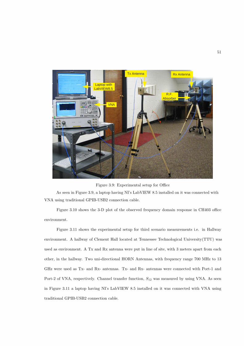
51
VNA
Tx Antenna
Laptop with LabVIEW8.5
Rx Antenna
R.F. Absorber
Figure 3.9: Experimental setup for Office
Figure 3.10 shows the 3-D plot of the observed frequency domain response in CH403 office
environment.
Figure 3.11 shows the experimental setup for third scenario measurements i.e. in Hallway
used as environment. A Tx and Rx antenna were put in line of site, with 3 meters apart from each
other, in the hallway. Two uni-directional HORN Antennas, with frequency range 700 MHz to 13
GHz were used as Tx- and Rx- antennas. Tx- and Rx- antennas were connected with Port-1 and
Port-2 of VNA, respectively. Channel transfer function, S12 was measured by using VNA. As seen
in Figure 3.11 a laptop having NI’s LabVIEW 8.5 installed on it was connected with VNA using
traditional GPIB-USB2 connection cable.
VNA using traditional GPIB-USB2 connection cable.
As seen in Figure 3.9, a laptop having NI’s LabVIEW 8.5 installed on it was connected with
environment. A hallway of Clement Hall located at Tennessee Technological University(TTU) was
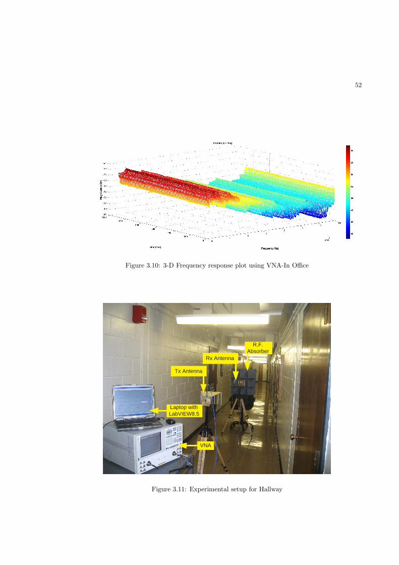
52
Figure 3.10: 3-D Frequency response plot using VNA-In Office
VNA
Tx Antenna
Laptop with LabVIEW8.5
Rx Antenna
R.F. Absorber
Figure 3.11: Experimental setup for Hallway
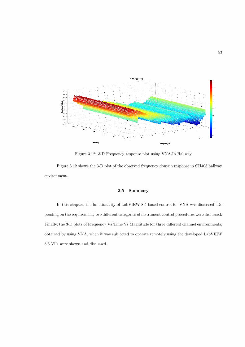
53
Figure 3.12: 3-D Frequency response plot using VNA-In Hallway
Figure 3.12 shows the 3-D plot of the observed frequency domain response in CH403 hallway
environment.
3.5 Summary
pending on the requirement, two different categories of instrument control procedures were discussed.
Finally, the 3-D plots of Frequency Vs Time Vs Magnitude for three different channel environments,
obtained by using VNA, when it was subjected to operate remotely using the developed LabVIEW
8.5 VI’s were shown and discussed.
In this chapter, the functionality of LabVIEW 8.5-based control for VNA was discussed. De-
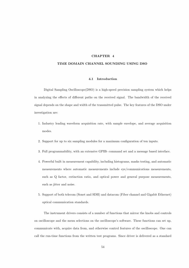
CHAPTER 4
TIME DOMAIN CHANNEL SOUNDING USING DSO
4.1 Introduction
Digital Sampling Oscilloscope(DSO) is a high-speed precision sampling system which helps
in analyzing the effects of different paths on the received signal. The bandwidth of the received
signal depends on the shape and width of the transmitted pulse. The key features of the DSO under
investigation are:
1. Industry leading waveform acquisition rate, with sample envelope, and average acquisition
modes.
2. Support for up to six sampling modules for a maximum configuration of ten inputs.
3. Full programmability, with an extensive GPIB- command set and a message based interface.
4. Powerful built in measurement capability, including histograms, masks testing, and automatic
measurements where automatic measurements include eye/communications measurements,
such as Q factor, extinction ratio, and optical power and general purpose measurements,
such as jitter and noise.
5. Support of both telecom (Sonet and SDH) and datacom (Fiber channel and Gigabit Ethernet)
optical communication standards.
The instrument drivers consists of a number of functions that mirror the knobs and controls
on oscilloscope and the menu selections on the oscilloscope’s software. These functions can set up,
communicate with, acquire data from, and otherwise control features of the oscilloscope. One can
call the run-time functions from the written test programs. Since driver is delivered as a standard
54
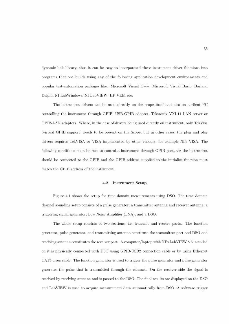
55
dynamic link library, thus it can be easy to incorporated these instrument driver functions into
programs that one builds using any of the following application development environments and
popular test-automation packages like: Microsoft Visual C++, Microsoft Visual Basic, Borland
Delphi, NI LabWindows, NI LabVIEW, HP VEE, etc.
The instrument drivers can be used directly on the scope itself and also on a client PC
controlling the instrument through GPIB, USB-GPIB adapter, Tektronix VXI-11 LAN server or
GPIB-LAN adapters. Where, in the case of drivers being used directly on instrument, only TekVisa
(virtual GPIB support) needs to be present on the Scope, but in other cases, the plug and play
drivers requires TekVISA or VISA implemented by other vendors, for example NI’s VISA. The
following conditions must be met to control a instrument through GPIB port, viz the instrument
should be connected to the GPIB and the GPIB address supplied to the initialize function must
match the GPIB address of the instrument.
4.2 Instrument Setup
Figure 4.1 shows the setup for time domain measurements using DSO. The time domain
channel sounding setup consists of a pulse generator, a transmitter antenna and receiver antenna, a
triggering signal generator, Low Noise Amplifier (LNA), and a DSO.
The whole setup consists of two sections, i.e, transmit and receive parts. The function
generator, pulse generator, and transmitting antenna constitute the transmitter part and DSO and
receiving antenna constitutes the receiver part. A computer/laptop with NI’s LabVIEW 8.5 installed
on it is physically connected with DSO using GPIB-USB2 connection cable or by using Ethernet
CAT5 cross cable. The function generator is used to trigger the pulse generator and pulse generator
generates the pulse that is transmitted through the channel. On the receiver side the signal is
received by receiving antenna and is passed to the DSO. The final results are displayed on the DSO
and LabVIEW is used to acquire measurement data automatically from DSO. A software trigger
56
Tx Antenna
Computer/Laptop with LabVIEW8.5
Rx Antenna
DSO Function
Generator
20dB Attenuation
GPIB-USB2 Connection
Cable
Pulse Generator
Figure 4.1: DSO Setup diagram
is used to reinitialize DSO after each set of measurement. The main advantages of time domain
channel sounding are less complexity, lower cost, and channel responses is readily available in time
domain.
The goal of this work is to get the time domain data of the frequently changing channel when
either the target is stationary or moving, for the future researchers to study the efficient channel
behavior. A 3-D plot showing Delay spread in seconds vs Amplitude in volts vs Time in seconds
(This is the time taken to complete each set of data acquisition) can be obtained by using this
approach.
Previously, DSO was controlled manually and the capability of getting time domain data
was limited. Now, LabVIEW is used to remotely control DSO. In this way, the semi-continuous
measurements can be done and the data can be recorded automatically in the form of text files, at
a desired location, on the remote computer’s hard disk.
In general, Tectronix8000B DSO has option for six sampling modules, out of which four
sampling modules has two inputs each and two sampling modules has one input each. This means
a DSO is capable of measuring time domain response of 10 channels at a time, whereas the DSO
57
4.3 Instrument Control using LabVIEW 8.5
LabVIEW-based instrument control project for DSO was subdivided into two categories as
mentioned below:
1. Save/Record measurement data in the form of a text file on local computer’s hard disk.
2. Acquire DSO screen/waveforms on the remote computer’s desktop using LabVIEW.
The first category was used to collect the time-domain measurement data for each channel,
remote terminal’s screen. Each waveform could be displayed individually on LabVIEW front panel.
As the DSO under inspection presently has four inputs installed on it, different LabVIEW
VI’s are developed to get time-domain data from each input, respectively, at same time. For example,
as in MIMO or SIMO cases multiple antennas are connected with each input at receiver end while
in SISO or MISO case only one antenna is connected with any one out of all available inputs.
Thus, depending on need, the DSO’s LabVIEW project contains different VI’s. This hierarchy
can be seen in Figure 1.4. These LabVIEW VI’s are named as:
1. DSO-1Channel-RecordData.vi
2. DSO-2Channels-RecordData.vi
3. DSO-3Channels-RecordData.vi
under investigation has two modules viz four inputs installed on it. Thus LabVIEW VIs’ are develo-
ped to measure the time domain response of the subjected environment either using all inputs at a
DSO depends on the nature of measurement techniques, i.e. SIMO or MIMO.
given time or by using set of any three, two, or one input at a given time. Selection of inputs on
while the second category set was used to view the time-domain waveforms as acquired by DSO on the
58
4. DSO-4Channels-RecordData.vi
5. DSO-1Channel-ViewTrace.vi
6. DSO-2Channels-ViewTrace.vi
7. DSO-3Channels-ViewTrace.vi
8. DSO-4Channels-ViewTrace.vi
Out of these eight VI’s, first four are used to record the data and time taken to collect each set
of data per iteration and next four are used to see the acquired waveforms on the remote computer
having LabVIEW installed on it.
4.3.1 To Save/Record Measurement Data
The working of LabVIEW VI for four channel inputs is as explained below. In this case,
observed time between two sets of measurements is around 3s by using GPIB-USB2 connection cable
and it reduces more significantly while using ethernet CAT5 Cross cable. One set of measurements
contains data for each channel input and a time stamp in millisecond value. Total time needed to
save time domain data includes DSO trigger time per channel, trace sweep time per channel, and
time required to record/save data files. In this way, more information about time domain response
can be obtained and extracted.
Figure 1.4 shows the LabVIEW project layout and Figure 4.3 shows the LabVIEW block
diagram to get time domain data using all inputs on DSO. The working of this VI is as explained
below.
1. Make tight connections as shown in Figure 4.1. Connection between PC and DSO can be
made possible by either GPIB-USB2 cable or by using CAT5 cross cable, depends on the
measurement requirements.
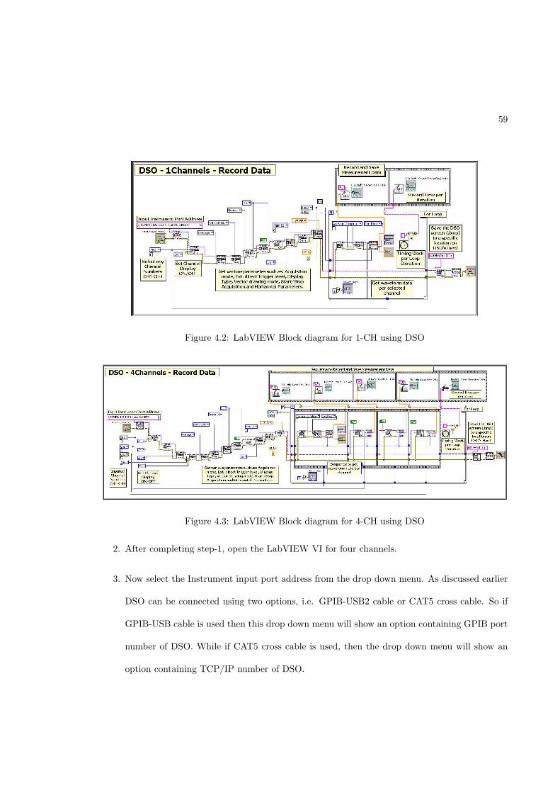
59
Figure 4.2: LabVIEW Block diagram for 1-CH using DSO
Figure 4.3: LabVIEW Block diagram for 4-CH using DSO
3. Now select the Instrument input port address from the drop down menu. As discussed earlier
DSO can be connected using two options, i.e. GPIB-USB2 cable or CAT5 cross cable. So if
GPIB-USB cable is used then this drop down menu will show an option containing GPIB port
number of DSO. While if CAT5 cross cable is used, then the drop down menu will show an
option containing TCP/IP number of DSO.
2. After completing step-1, open the LabVIEW VI for four channels.
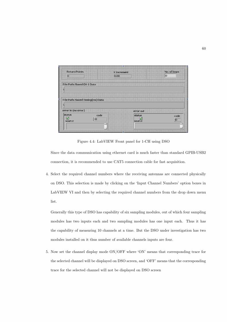
60
Figure 4.4: LabVIEW Front panel for 1-CH using DSO
Since the data communication using ethernet card is much faster than standard GPIB-USB2
connection, it is recommended to use CAT5 connection cable for fast acquisition.
4. Select the required channel numbers where the receiving antennas are connected physically
on DSO. This selection is made by clicking on the ‘Input Channel Numbers’ option boxes in
LabVIEW VI and then by selecting the required channel numbers from the drop down menu
list.
Generally this type of DSO has capability of six sampling modules, out of which four sampling
modules has two inputs each and two sampling modules has one input each. Thus it has
the capability of measuring 10 channels at a time. But the DSO under investigation has two
modules installed on it thus number of available channels inputs are four.
5. Now set the channel display mode ON/OFF where ‘ON’ means that corresponding trace for
the selected channel will be displayed on DSO screen, and ‘OFF’ means that the corresponding
trace for the selected channel will not be displayed on DSO screen
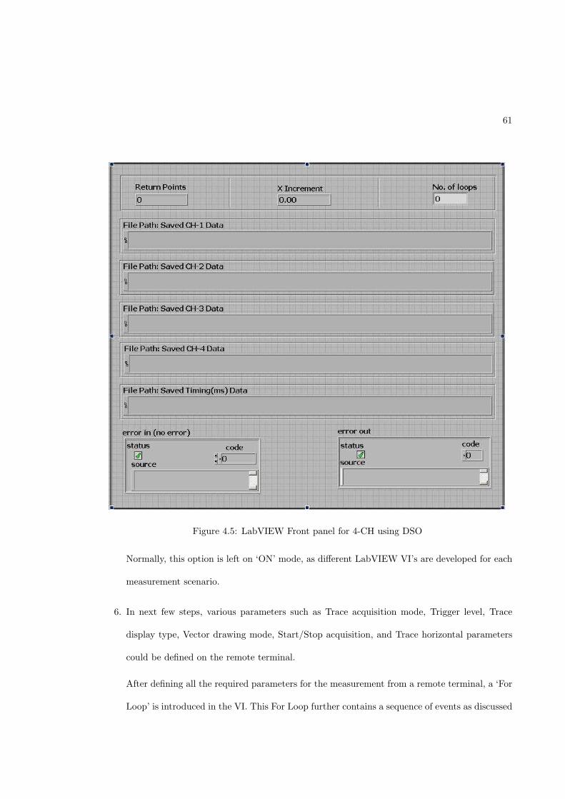
61
Figure 4.5: LabVIEW Front panel for 4-CH using DSO
Normally, this option is left on ‘ON’ mode, as different LabVIEW VI’s are developed for each
measurement scenario.
6. In next few steps, various parameters such as Trace acquisition mode, Trigger level, Trace
display type, Vector drawing mode, Start/Stop acquisition, and Trace horizontal parameters
could be defined on the remote terminal.
After defining all the required parameters for the measurement from a remote terminal, a ‘For
Loop’ is introduced in the VI. This For Loop further contains a sequence of events as discussed
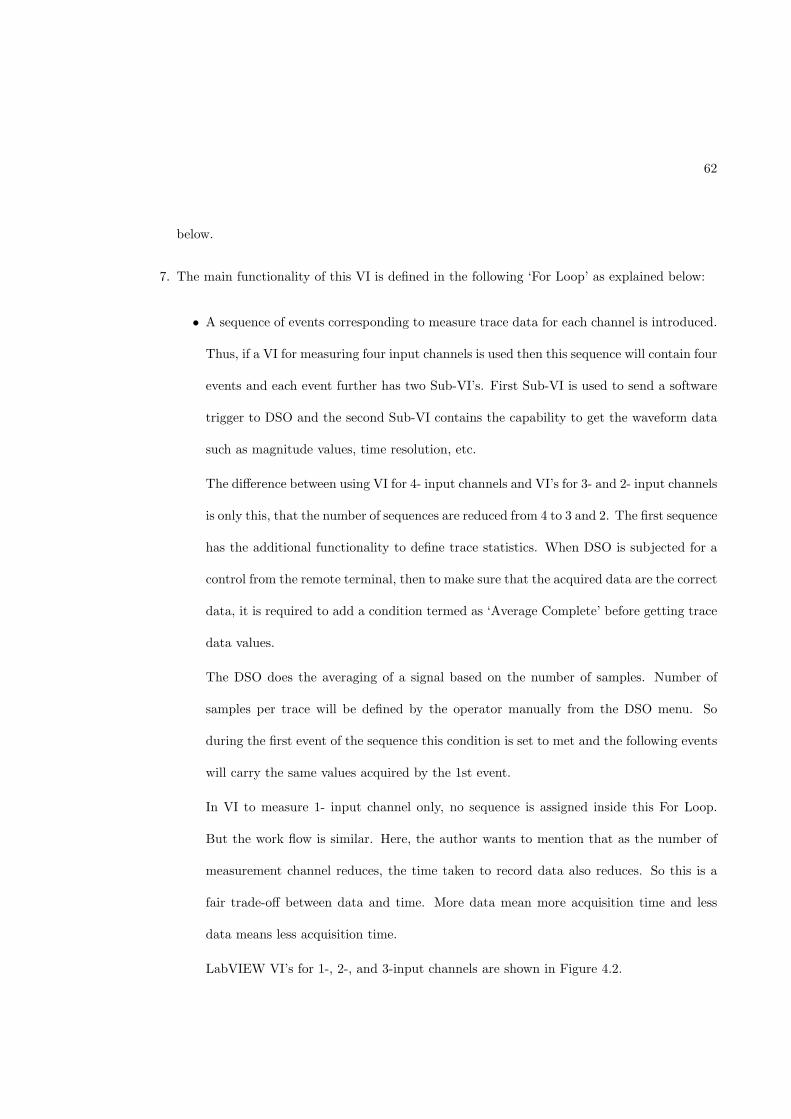
62
below.
7. The main functionality of this VI is defined in the following ‘For Loop’ as explained below:
• A sequence of events corresponding to measure trace data for each channel is introduced.
Thus, if a VI for measuring four input channels is used then this sequence will contain four
events and each event further has two Sub-VI’s. First Sub-VI is used to send a software
trigger to DSO and the second Sub-VI contains the capability to get the waveform data
such as magnitude values, time resolution, etc.
The difference between using VI for 4- input channels and VI’s for 3- and 2- input channels
is only this, that the number of sequences are reduced from 4 to 3 and 2. The first sequence
has the additional functionality to define trace statistics. When DSO is subjected for a
control from the remote terminal, then to make sure that the acquired data are the correct
data, it is required to add a condition termed as ‘Average Complete’ before getting trace
data values.
The DSO does the averaging of a signal based on the number of samples. Number of
samples per trace will be defined by the operator manually from the DSO menu. So
during the first event of the sequence this condition is set to met and the following events
will carry the same values acquired by the 1st event.
In VI to measure 1- input channel only, no sequence is assigned inside this For Loop.
But the work flow is similar. Here, the author wants to mention that as the number of
measurement channel reduces, the time taken to record data also reduces. So this is a
fair trade-off between data and time. More data mean more acquisition time and less
data means less acquisition time.
LabVIEW VI’s for 1-, 2-, and 3-input channels are shown in Figure 4.2.
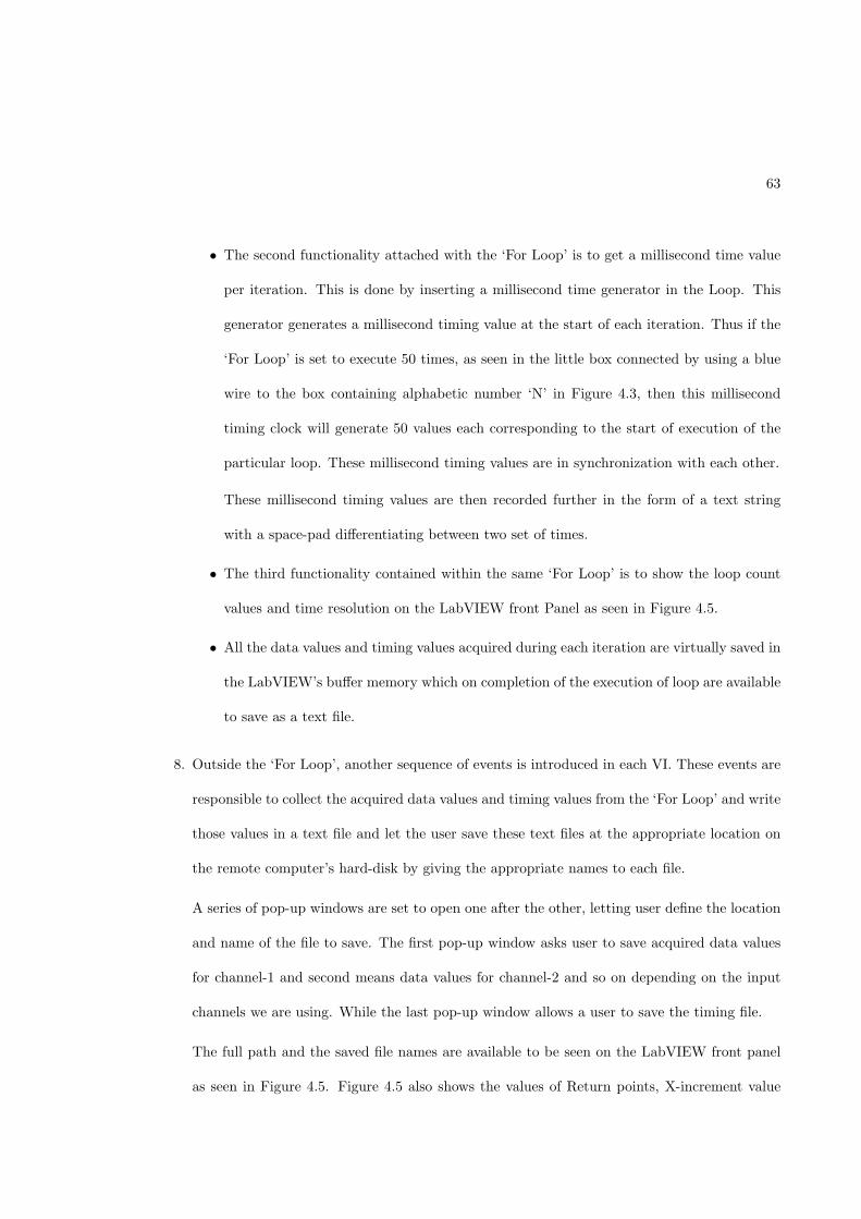
63
• The second functionality attached with the ‘For Loop’ is to get a millisecond time value
per iteration. This is done by inserting a millisecond time generator in the Loop. This
generator generates a millisecond timing value at the start of each iteration. Thus if the
‘For Loop’ is set to execute 50 times, as seen in the little box connected by using a blue
wire to the box containing alphabetic number ‘N’ in Figure 4.3, then this millisecond
timing clock will generate 50 values each corresponding to the start of execution of the
particular loop. These millisecond timing values are in synchronization with each other.
These millisecond timing values are then recorded further in the form of a text string
with a space-pad differentiating between two set of times.
• The third functionality contained within the same ‘For Loop’ is to show the loop count
values and time resolution on the LabVIEW front Panel as seen in Figure 4.5.
• All the data values and timing values acquired during each iteration are virtually saved in
the LabVIEW’s buffer memory which on completion of the execution of loop are available
to save as a text file.
8. Outside the ‘For Loop’, another sequence of events is introduced in each VI. These events are
responsible to collect the acquired data values and timing values from the ‘For Loop’ and write
those values in a text file and let the user save these text files at the appropriate location on
the remote computer’s hard-disk by giving the appropriate names to each file.
A series of pop-up windows are set to open one after the other, letting user define the location
and name of the file to save. The first pop-up window asks user to save acquired data values
for channel-1 and second means data values for channel-2 and so on depending on the input
channels we are using. While the last pop-up window allows a user to save the timing file.
The full path and the saved file names are available to be seen on the LabVIEW front panel
as seen in Figure 4.5. Figure 4.5 also shows the values of Return points, X-increment value
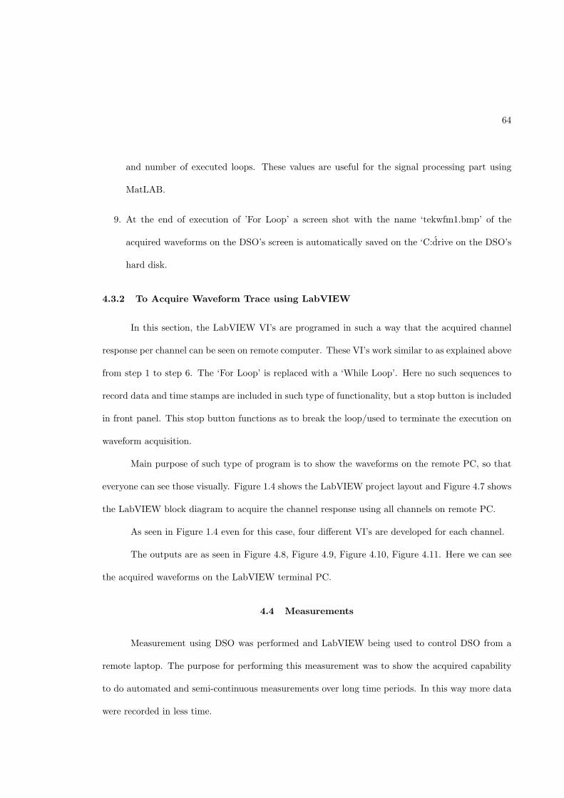
64
and number of executed loops. These values are useful for the signal processing part using
MatLAB.
9. At the end of execution of ’For Loop’ a screen shot with the name ‘tekwfm1.bmp’ of the
acquired waveforms on the DSO’s screen is automatically saved on the ‘C:drive on the DSO’s
hard disk.
4.3.2 To Acquire Waveform Trace using LabVIEW
In this section, the LabVIEW VI’s are programed in such a way that the acquired channel
response per channel can be seen on remote computer. These VI’s work similar to as explained above
from step 1 to step 6. The ‘For Loop’ is replaced with a ‘While Loop’. Here no such sequences to
record data and time stamps are included in such type of functionality, but a stop button is included
in front panel. This stop button functions as to break the loop/used to terminate the execution on
waveform acquisition.
Main purpose of such type of program is to show the waveforms on the remote PC, so that
everyone can see those visually. Figure 1.4 shows the LabVIEW project layout and Figure 4.7 shows
the LabVIEW block diagram to acquire the channel response using all channels on remote PC.
As seen in Figure 1.4 even for this case, four different VI’s are developed for each channel.
The outputs are as seen in Figure 4.8, Figure 4.9, Figure 4.10, Figure 4.11. Here we can see
the acquired waveforms on the LabVIEW terminal PC.
4.4 Measurements
Measurement using DSO was performed and LabVIEW being used to control DSO from a
remote laptop. The purpose for performing this measurement was to show the acquired capability
to do automated and semi-continuous measurements over long time periods. In this way more data
were recorded in less time.
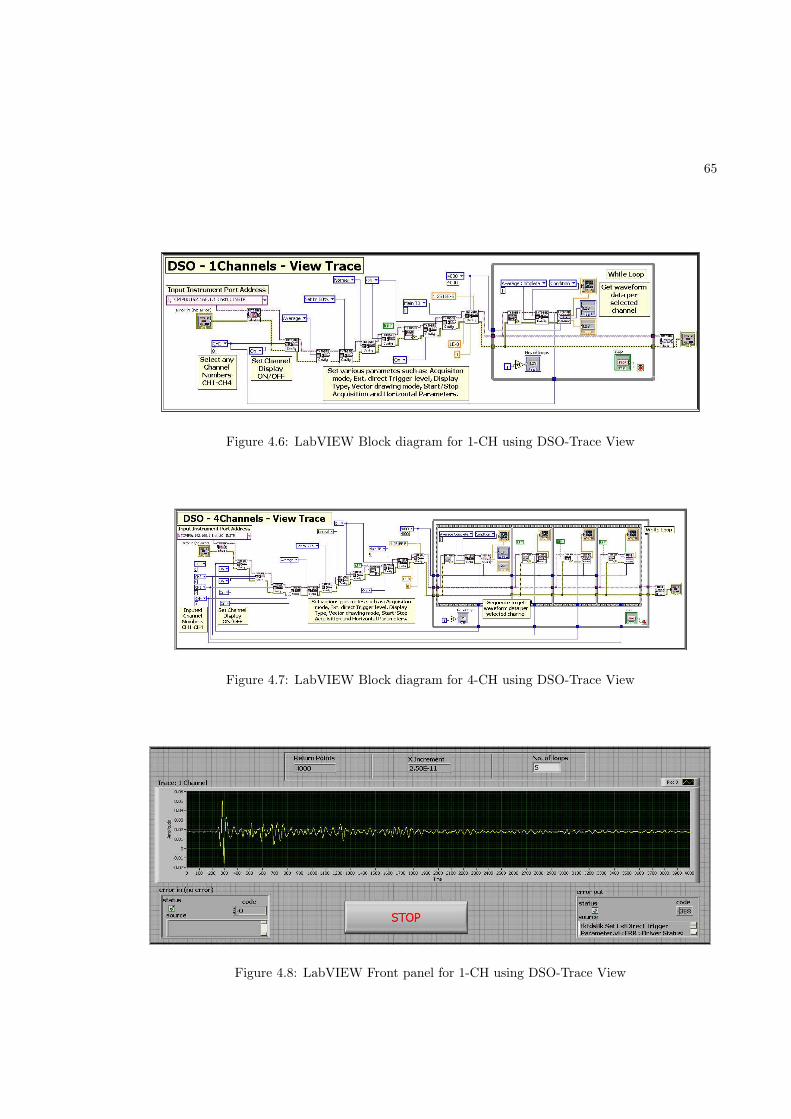
65
Figure 4.6: LabVIEW Block diagram for 1-CH using DSO-Trace View
Figure 4.7: LabVIEW Block diagram for 4-CH using DSO-Trace View
Figure 4.8: LabVIEW Front panel for 1-CH using DSO-Trace View

66
Figure 4.9: LabVIEW Front panel for 2-CH using DSO
Figure 4.10: LabVIEW Front panel for 3-CH using DSO
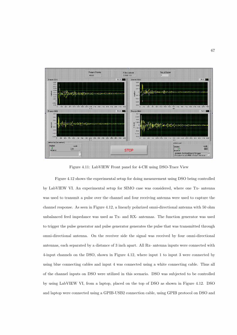
67
Figure 4.11: LabVIEW Front panel for 4-CH using DSO-Trace View
Figure 4.12 shows the experimental setup for doing measurement using DSO being controlled
by LabVIEW VI. An experimental setup for SIMO case was considered, where one Tx- antenna
was used to transmit a pulse over the channel and four receiving antenna were used to capture the
channel response. As seen in Figure 4.12, a linearly polarized omni-directional antenna with 50 ohm
unbalanced feed impedance was used as Tx- and RX- antennas. The function generator was used
to trigger the pulse generator and pulse generator generates the pulse that was transmitted through
omni-directional antenna. On the receiver side the signal was received by four omni-directional
antennas, each separated by a distance of 3 inch apart. All Rx- antenna inputs were connected with
4-input channels on the DSO, shown in Figure 4.12, where input 1 to input 3 were connected by
using blue connecting cables and input 4 was connected using a white connecting cable. Thus all
of the channel inputs on DSO were utilized in this scenario. DSO was subjected to be controlled
by using LabVIEW VI, from a laptop, placed on the top of DSO as shown in Figure 4.12. DSO
and laptop were connected using a GPIB-USB2 connection cable, using GPIB protocol on DSO and
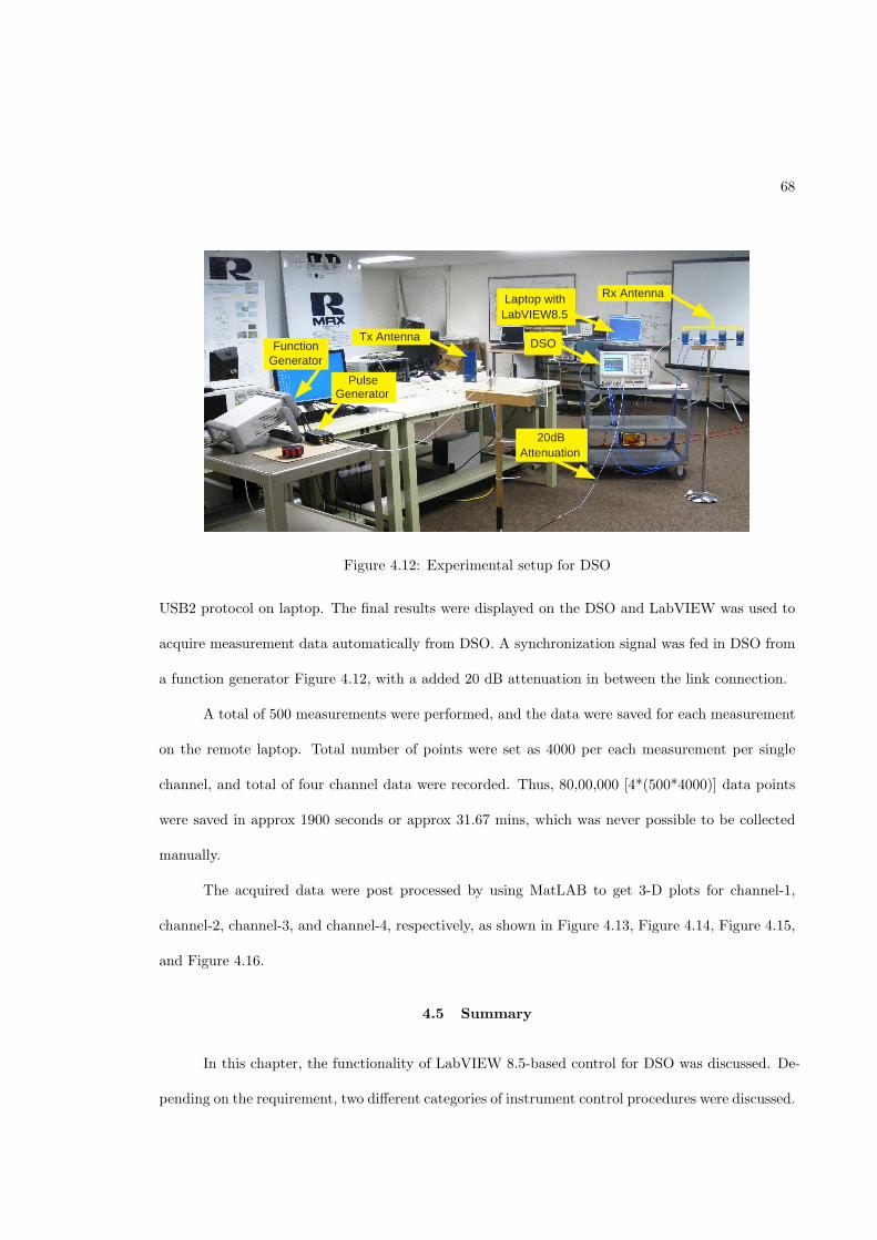
68
Pulse Generator
Tx Antenna
Laptop with LabVIEW8.5
Rx Antenna
DSO Function Generator
20dB Attenuation
Figure 4.12: Experimental setup for DSO
USB2 protocol on laptop. The final results were displayed on the DSO and LabVIEW was used to
acquire measurement data automatically from DSO. A synchronization signal was fed in DSO from
a function generator Figure 4.12, with a added 20 dB attenuation in between the link connection.
A total of 500 measurements were performed, and the data were saved for each measurement
on the remote laptop. Total number of points were set as 4000 per each measurement per single
channel, and total of four channel data were recorded. Thus, 80,00,000 [4*(500*4000)] data points
were saved in approx 1900 seconds or approx 31.67 mins, which was never possible to be collected
manually.
The acquired data were post processed by using MatLAB to get 3-D plots for channel-1,
channel-2, channel-3, and channel-4, respectively, as shown in Figure 4.13, Figure 4.14, Figure 4.15,
and Figure 4.16.
4.5 Summary
pending on the requirement, two different categories of instrument control procedures were discussed.
In this chapter, the functionality of LabVIEW 8.5-based control for DSO was discussed. De-
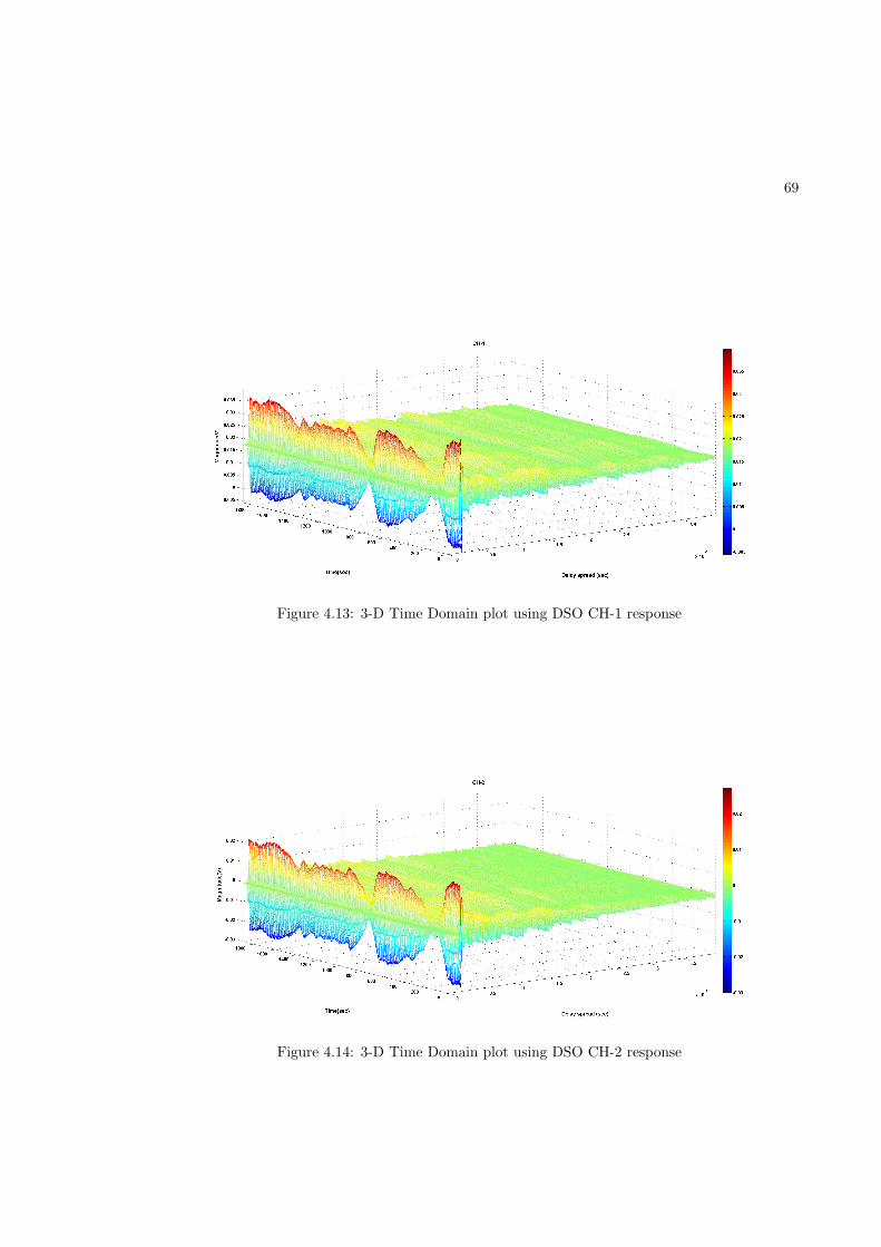
69
Figure 4.13: 3-D Time Domain plot using DSO CH-1 response
Figure 4.14: 3-D Time Domain plot using DSO CH-2 response
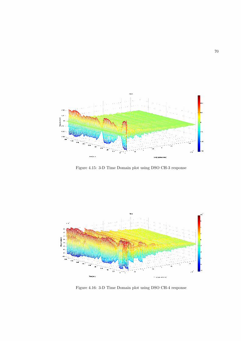
70
Figure 4.15: 3-D Time Domain plot using DSO CH-3 response
Figure 4.16: 3-D Time Domain plot using DSO CH-4 response

71
Finally, the 3-D plots of Delay Spread Vs Time Vs Amplitude for four different channels were shown,
when DSO was subjected to operate remotely using the developed LabVIEW 8.5 VI’s.
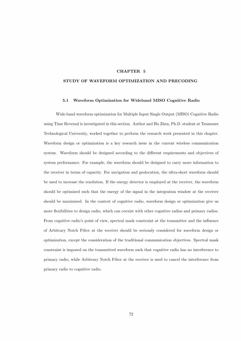
CHAPTER 5
STUDY OF WAVEFORM OPTIMIZATION AND PRECODING
5.1 Waveform Optimization for Wideband MISO Cognitive Radio
Wide-band waveform optimization for Multiple Input Single Output (MISO) Cognitive Radio
using Time Reversal is investigated in this section. Author and Hu Zhen, Ph.D. student at Tennessee
Technological University, worked together to perform the research work presented in this chapter.
Waveform design or optimization is a key research issue in the current wireless communication
system. Waveform should be designed according to the different requirements and objectives of
system performance. For example, the waveform should be designed to carry more information to
the receiver in terms of capacity. For navigation and geolocation, the ultra-short waveform should
be used to increase the resolution. If the energy detector is employed at the receiver, the waveform
should be optimized such that the energy of the signal in the integration window at the receiver
should be maximized. In the context of cognitive radio, waveform design or optimization give us
more flexibilities to design radio, which can coexist with other cognitive radios and primary radios.
From cognitive radio’s point of view, spectral mask constraint at the transmitter and the influence
of Arbitrary Notch Filter at the receiver should be seriously considered for waveform design or
optimization, except the consideration of the traditional communication objectives. Spectral mask
constraint is imposed on the transmitted waveform such that cognitive radio has no interference to
primary radio, while Arbitrary Notch Filter at the receiver is used to cancel the interference from
primary radio to cognitive radio.
72
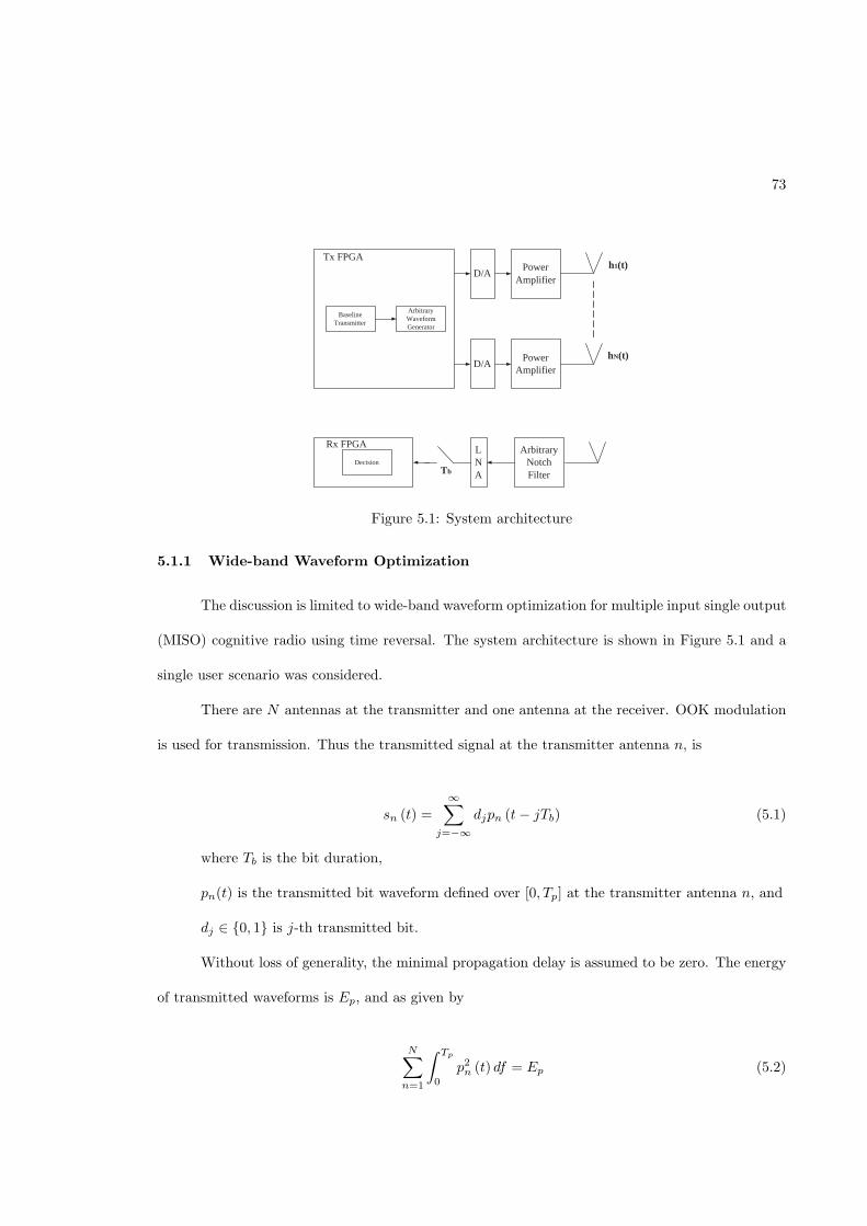
73
Baseline Transmitter
Arbitrary Waveform Generator
Tx FPGA
D/A Power
Amplifier
Rx FPGA L N A
Arbitrary Notch Filter
D/A Power
Amplifier
T b Decision
h 1 (t)
h N (t)
Figure 5.1: System architecture
5.1.1 Wide-band Waveform Optimization
The discussion is limited to wide-band waveform optimization for multiple input single output
(MISO) cognitive radio using time reversal. The system architecture is shown in Figure 5.1 and a
single user scenario was considered.
There are N antennas at the transmitter and one antenna at the receiver. OOK modulation
is used for transmission. Thus the transmitted signal at the transmitter antenna n, is
sn (t) =
∞∑
j=−∞
djpn (t − jTb) (5.1)
where Tb is the bit duration,
n p
dj ∈ {0, 1} is j-th transmitted bit.
Without loss of generality, the minimal propagation delay is assumed to be zero. The energy
of transmitted waveforms is Ep, and as given by
N∑
n=1
∫ Tp
0
p2n (t) df = Ep (5.2)
p (t) is the transmitted bit waveform defined over [0, T ] at the transmitter antenna n, and
74
The received noise-polluted signal at the output of low noise amplifier (LNA) is
r(t) =
N∑
n=1
hn (t) ⊗ sn (t) + n (t) (5.3)
=
∞∑
j=−∞
dj
N∑
n=1
xn (t − jTb) + n (t) (5.4)
where hn (t) , t ∈ [0, Th] is the multi-path impulse response that takes into account the effect
of channel impulse response, the RF front-ends in the transceivers such as Power Amplifier, LNA
and Arbitrary Notch Filter, as well as antennas between the transmitter antenna n and the receiver
antenna.
hn(t) is available at the transmitter, as given by
∫ Th
0h2
n (t) dt = Enh.
If “⊗” denotes convolution operation.
n(t) is AWGN and
xn(t) is the received noiseless bit-“1”
then waveform defined as
xn(t) = hn(t) ⊗ pn(t) (5.5)
It is assumed that Tb ≥ Th + Tp
def= Tx, i.e. no existence of ISI.
If the waveforms at different transmitter antennas are assumed to be synchronized, the k-th
decision statistic is
r(kTb + t0) =
∞∑
j=−∞
dj
N∑
n=1
xn (kTb + t0 − jTb) + n (t) (5.6)
= dk
N∑
n=1
xn (t0) + n (t) (5.7)
75
In order to maximize the system performance,N∑
n=1xn (t0) should be maximized. Thus the
optimization problem can be formulated as follows to get the optimal waveforms pn(t).
maxN∑
n=1xn (t0)
s.t.N∑
n=1
∫ Tp
0p2
n (t) df ≤ Ep
0 ≤ t0 ≤ Tb
(5.8)
An iterative algorithm was proposed here to give the optimal solution to the optimization
problem 5.8, which was a computationally-efficient algorithm. For the simplicity of the following
presentation, t0 is assumed to be zero. Meanwhile,
x (t) =
N∑
n=1
xn (t) (5.9)
From inverse Fourier transform,
xnf (f) = hnf (f) pnf (f) (5.10)
and
xf (f) =
N∑
n=1
hnf (f) pnf (f) (5.11)
and pn(t), respectively.
xf (f) is frequency domain representation of x(t). Thus,
x (0) =N
∑
n=1
xn (0) (5.12)
and
xn (0) =
∫
∞
−∞
xnf (f) df (5.13)
where x (f), h (f), and p (f) are the frequency domain representations of x (t), h (t),nf nf nf n n
76
If there is no spectral mask constraint, then according to the Cauchy−Schwarz inequality,
x (0) =
N∑
n=1
∫
∞
−∞
hnf (f) pnf (f) df (5.14)
≤N
∑
n=1
√
∫
∞
−∞
|hnf (f)|2 df
∫
∞
−∞
|pnf (f)|2 df (5.15)
≤
√
√
√
√
N∑
n=1
∫
∞
−∞
|hnf (f)|2 df
√
√
√
√
N∑
n=1
∫
∞
−∞
|pnf (f)|2 df (5.16)
=
√
√
√
√Ep
N∑
n=1
Enh (5.17)
when pnf (f) = αhnf (f) for all f and n, two equalities are obtained.
α =
√
√
√
√
√
Ep
N∑
n=1
∫
∞
−∞|hnf (f)|2 df
(5.18)
In this case, pn (t) = αhn (−t), which means the optimal waveform pn(t) is the corresponding
time reversed multipath impulse response hn(t).
If there is spectral mask constraint, then the following optimization problem will become
more complicated,
max x (0)
s.t.N∑
n=1
∫ Tp
0p2
n (t) df ≤ Ep
|pnf (f)|2 ≤ cnf (f)
(5.19)
where cnf (f) represents the arbitrary spectral mask constraint at the transmitter antenna n.
Because pnf (f) is the complex value, the phase and the modulus of pnf (f) should be deter-
mined.
Meanwhile,
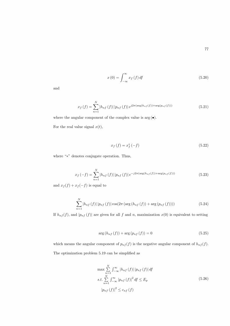
77
x (0) =
∫
∞
−∞
xf (f) df (5.20)
and
xf (f) =N
∑
n=1
|hnf (f)| |pnf (f)| ej2π(arg(hnf (f))+arg(pnf (f))) (5.21)
where the angular component of the complex value is arg (•).
For the real value signal x(t),
xf (f) = x∗
f (−f) (5.22)
where “∗” denotes conjugate operation. Thus,
xf (−f) =
N∑
n=1
|hnf (f)| |pnf (f)| e−j2π(arg(hnf (f))+arg(pnf (f))) (5.23)
and xf (f) + xf (−f) is equal to
N∑
n=1
|hnf (f)| |pnf (f)| cos(2π (arg (hnf (f)) + arg (pnf (f)))) (5.24)
If hnf (f), and |pnf (f)| are given for all f and n, maximization x(0) is equivalent to setting
arg (hnf (f)) + arg (pnf (f)) = 0 (5.25)
which means the angular component of pnf (f) is the negative angular component of hnf (f).
The optimization problem 5.19 can be simplified as
maxN∑
n=1
∫
∞
−∞|hnf (f)| |pnf (f)| df
s.t.N∑
n=1
∫
∞
−∞|pnf (f)|2 df ≤ Ep
|pnf (f)|2 ≤ cnf (f)
(5.26)
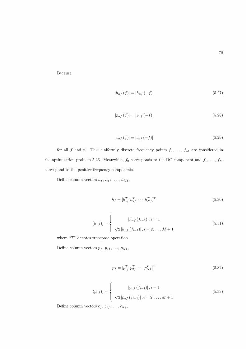
78
Because
|hnf (f)| = |hnf (−f)| (5.27)
|pnf (f)| = |pnf (−f)| (5.28)
|cnf (f)| = |cnf (−f)| (5.29)
for all f and n. Thus uniformly discrete frequency points f0, . . ., fM are considered in
the optimization problem 5.26. Meanwhile, f0 corresponds to the DC component and f1, . . ., fM
correspond to the positive frequency components.
Define column vectors hf , h1f , . . ., hNf ,
hf = [hT1f hT
2f · · · hTNf ]T (5.30)
(hnf )i=
|hnf (fi−1)| , i = 1
√2 |hnf (fi−1)| , i = 2, . . . ,M + 1
(5.31)
where “T” denotes transpose operation
Define column vectors pf , p1f , . . ., pNf ,
pf = [pT1f pT
2f · · · pTNf ]T (5.32)
(pnf )i=
|pnf (fi−1)| , i = 1
√2 |pnf (fi−1)| , i = 2, . . . ,M + 1
(5.33)
Define column vectors cf , c1f , . . ., cNf ,
79
cf = [cT1f cT
2f · · · cTNf ]T (5.34)
(cnf )i=
√
|cnf (fi−1)|, i = 1
√
2 |cnf (fi−1)|, i = 2, . . . ,M + 1
(5.35)
Thus, the discrete version of the optimization problem 5.26 is shown below.
max hTf pf
s.t. ‖pf‖22 ≤ Ep
0 ≤ pf ≤ cf
(5.36)
An iterative algorithm is shown as follows.
1. Initialization: P = Ep and p∗f is set to be all-0 column vector.
2. Solve the following optimization problem to get the optimal q∗f using Cauchy−Schwarz in-
equality.
max hTf qf
s.t. ‖qf‖22 ≤ P
(5.37)
3. Find i, such that(
q∗f
)
iis the maximal value in the set
{
(
q∗f
)
j
∣
∣
∣
∣
(
q∗f
)
j> (cf )
j
}
. If {i} = ∅,
then the algorithm is terminated and p∗f := p∗f + q∗f . Otherwise go to step 4.
4. Set(
p∗f
)
i= (cf )
i.
5. P := P − (cf )2i
and set (hf )i
to zero. Go to step 2.
When p∗f is obtained for the optimization problem 5.36, from Equation 5.25, Equation 5.32,
and Equation 5.33, the optimal pnf (f) and the corresponding pn(t) can be smoothly achieved.
80
0 2 4 6 8 10
x 109
0
0.005
0.01
0.015
0.02
0.025
0.03
Frequency (Hz)
Mag
nitu
de
Figure 5.2: Channel Transfer function between the first transmitter antenna and the receiver antenna
0 2 4 6 8 10
x 109
0
0.005
0.01
0.015
0.02
0.025
0.03
Frequency (Hz)
Mag
nitu
de
Figure 5.3: Channel transfer function between the second transmitter antenna and the receiverantenna.
5.1.2 Numerical Results
The channel impulse responses, in Rectangular Metal Cavity was used as an example to show
the results of the wide-band waveform optimization for MISO cognitive radio using time reversal.
N = 3. The measured frequency band is from 3GHz to 10GHz. Figure 5.2, Figure 5.3, and
are all normalized.
Because of the interference at the receiver, it was assumed that Arbitrary Notch Filter will
notch the frequency band from 5GHz to 6GHz and the frequency band from 8GHz to 9GHz.
Figure 5.4 show channel transfer functions, respectively. Figure 5.5, Figure 5.6, and Figure 5.7 show
the corresponding channel impulse responses, respectively. The energies of channel impulse responses
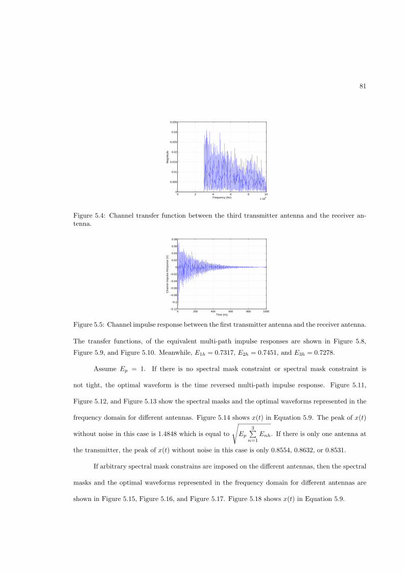
81
0 2 4 6 8 10
x 109
0
0.005
0.01
0.015
0.02
0.025
0.03
0.035
Frequency (Hz)
Mag
nitu
de
Figure 5.4: Channel transfer function between the third transmitter antenna and the receiver an-tenna.
0 200 400 600 800 1000−0.12
−0.1
−0.08
−0.06
−0.04
−0.02
0
0.02
0.04
0.06
0.08
Time (ns)
Cha
nnel
Impu
lse
Res
pons
e (V
)
Figure 5.5: Channel impulse response between the first transmitter antenna and the receiver antenna.
Figure 5.9, and Figure 5.10. Meanwhile, E1h = 0.7317, E2h = 0.7451, and E3h = 0.7278.
Assume Ep = 1. If there is no spectral mask constraint or spectral mask constraint is
not tight, the optimal waveform is the time reversed multi-path impulse response. Figure 5.11,
Figure 5.12, and Figure 5.13 show the spectral masks and the optimal waveforms represented in the
frequency domain for different antennas. Figure 5.14 shows x(t) in Equation 5.9. The peak of x(t)
without noise in this case is 1.4848 which is equal to
√
Ep
3∑
n=1Enh. If there is only one antenna at
the transmitter, the peak of x(t) without noise in this case is only 0.8554, 0.8632, or 0.8531.
If arbitrary spectral mask constrains are imposed on the different antennas, then the spectral
masks and the optimal waveforms represented in the frequency domain for different antennas are
shown in Figure 5.15, Figure 5.16, and Figure 5.17. Figure 5.18 shows x(t) in Equation 5.9.
The transfer functions, of the equivalent multi-path impulse responses are shown in Figure 5.8,
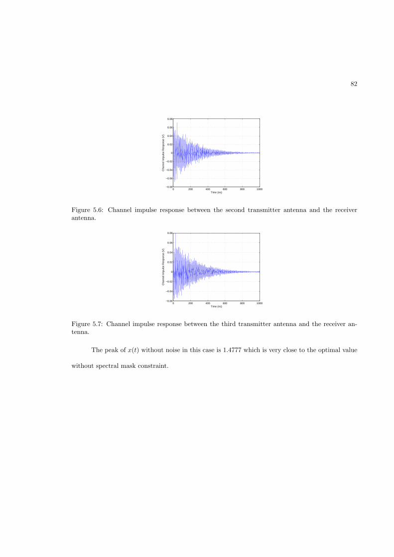
82
0 200 400 600 800 1000−0.08
−0.06
−0.04
−0.02
0
0.02
0.04
0.06
0.08
Time (ns)
Cha
nnel
Impu
lse
Res
pons
e (V
)
Figure 5.6: Channel impulse response between the second transmitter antenna and the receiverantenna.
0 200 400 600 800 1000−0.06
−0.04
−0.02
0
0.02
0.04
0.06
0.08
Time (ns)
Cha
nnel
Impu
lse
Res
pons
e (V
)
Figure 5.7: Channel impulse response between the third transmitter antenna and the receiver an-tenna.
The peak of x(t) without noise in this case is 1.4777 which is very close to the optimal value
without spectral mask constraint.
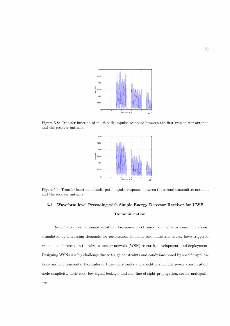
83
0 2 4 6 8 10
x 109
0
0.005
0.01
0.015
0.02
0.025
0.03
Frequency (Hz)
Mag
nitu
de
Figure 5.8: Transfer function of multi-path impulse response between the first transmitter antennaand the receiver antenna.
0 2 4 6 8 10
x 109
0
0.005
0.01
0.015
0.02
0.025
0.03
Frequency (Hz)
Mag
nitu
de
Figure 5.9: Transfer function of multi-path impulse response between the second transmitter antennaand the receiver antenna.
5.2 Waveform-level Precoding with Simple Energy Detector Receiver for UWB
Communication
Recent advances in miniaturization, low-power electronics, and wireless communications,
stimulated by increasing demands for automation in home and industrial areas, have triggered
tremendous interests in the wireless sensor network (WSN) research, development, and deployment.
Designing WSNs is a big challenge due to tough constraints and conditions posed by specific applica-
tions and environments. Examples of these constraints and conditions include power consumption,
node simplicity, node cost, low signal leakage, and non-line-of-sight propagation, severe multipath,
etc.
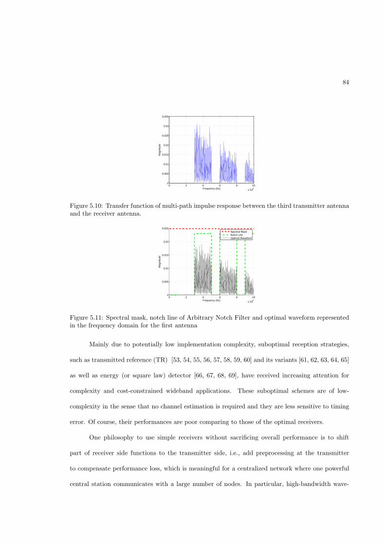
84
0 2 4 6 8 10
x 109
0
0.005
0.01
0.015
0.02
0.025
0.03
0.035
Frequency (Hz)
Mag
nitu
de
Figure 5.10: Transfer function of multi-path impulse response between the third transmitter antennaand the receiver antenna.
0 2 4 6 8 10
x 109
0
0.005
0.01
0.015
0.02
0.025
Frequency (Hz)
Mag
nitu
de
Spectral MaskNotch LineOptimal Waveform
Figure 5.11: Spectral mask, notch line of Arbitrary Notch Filter and optimal waveform representedin the frequency domain for the first antenna
Mainly due to potentially low implementation complexity, suboptimal reception strategies,
such as transmitted reference (TR) [53, 54, 55, 56, 57, 58, 59, 60] and its variants [61, 62, 63, 64, 65]
as well as energy (or square law) detector [66, 67, 68, 69], have received increasing attention for
complexity and cost-constrained wideband applications. These suboptimal schemes are of low-
complexity in the sense that no channel estimation is required and they are less sensitive to timing
error. Of course, their performances are poor comparing to those of the optimal receivers.
One philosophy to use simple receivers without sacrificing overall performance is to shift
part of receiver side functions to the transmitter side, i.e., add preprocessing at the transmitter
to compensate performance loss, which is meaningful for a centralized network where one powerful
central station communicates with a large number of nodes. In particular, high-bandwidth wave-
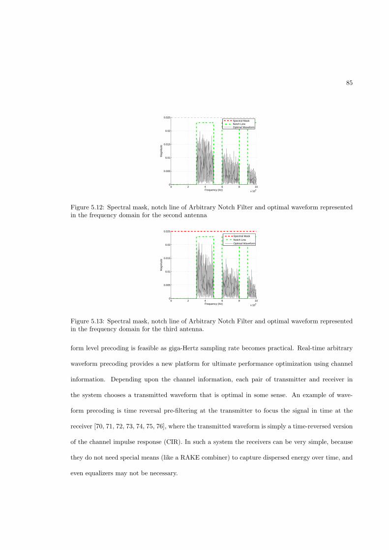
85
0 2 4 6 8 10
x 109
0
0.005
0.01
0.015
0.02
0.025
Frequency (Hz)
Mag
nitu
de
Spectral MaskNotch LineOptimal Waveform
Figure 5.12: Spectral mask, notch line of Arbitrary Notch Filter and optimal waveform representedin the frequency domain for the second antenna
0 2 4 6 8 10
x 109
0
0.005
0.01
0.015
0.02
0.025
Frequency (Hz)
Mag
nitu
de
Spectral MaskNotch LineOptimal Waveform
Figure 5.13: Spectral mask, notch line of Arbitrary Notch Filter and optimal waveform representedin the frequency domain for the third antenna.
form level precoding is feasible as giga-Hertz sampling rate becomes practical. Real-time arbitrary
waveform precoding provides a new platform for ultimate performance optimization using channel
information. Depending upon the channel information, each pair of transmitter and receiver in
the system chooses a transmitted waveform that is optimal in some sense. An example of wave-
form precoding is time reversal pre-filtering at the transmitter to focus the signal in time at the
receiver [70, 71, 72, 73, 74, 75, 76], where the transmitted waveform is simply a time-reversed version
of the channel impulse response (CIR). In such a system the receivers can be very simple, because
they do not need special means (like a RAKE combiner) to capture dispersed energy over time, and
even equalizers may not be necessary.
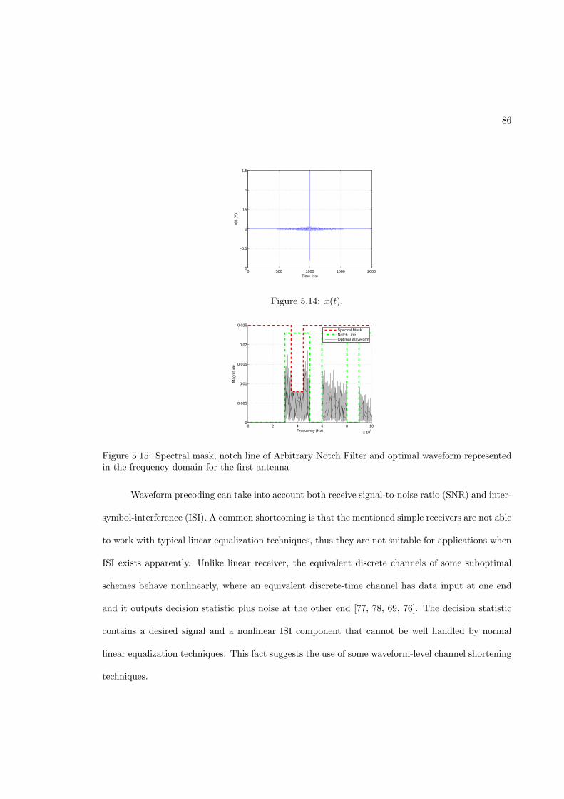
86
0 500 1000 1500 2000−1
−0.5
0
0.5
1
1.5
Time (ns)
x(t)
(V
)
Figure 5.14: x(t).
0 2 4 6 8 10
x 109
0
0.005
0.01
0.015
0.02
0.025
Frequency (Hz)
Mag
nitu
de
Spectral MaskNotch LineOptimal Waveform
Figure 5.15: Spectral mask, notch line of Arbitrary Notch Filter and optimal waveform representedin the frequency domain for the first antenna
Waveform precoding can take into account both receive signal-to-noise ratio (SNR) and inter-
symbol-interference (ISI). A common shortcoming is that the mentioned simple receivers are not able
to work with typical linear equalization techniques, thus they are not suitable for applications when
ISI exists apparently. Unlike linear receiver, the equivalent discrete channels of some suboptimal
schemes behave nonlinearly, where an equivalent discrete-time channel has data input at one end
and it outputs decision statistic plus noise at the other end [77, 78, 69, 76]. The decision statistic
contains a desired signal and a nonlinear ISI component that cannot be well handled by normal
linear equalization techniques. This fact suggests the use of some waveform-level channel shortening
techniques.
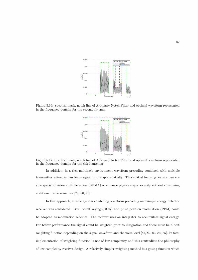
87
0 2 4 6 8 10
x 109
0
0.005
0.01
0.015
0.02
0.025
Frequency (Hz)
Mag
nitu
de
Spectral MaskNotch LineOptimal Waveform
Figure 5.16: Spectral mask, notch line of Arbitrary Notch Filter and optimal waveform representedin the frequency domain for the second antenna
0 2 4 6 8 10
x 109
0
0.005
0.01
0.015
0.02
0.025
Frequency (Hz)
Mag
nitu
de
Spectral MaskNotch LineOptimal Waveform
Figure 5.17: Spectral mask, notch line of Arbitrary Notch Filter and optimal waveform representedin the frequency domain for the third antenna
transmitter antennas can focus signal into a spot spatially. This spatial focusing feature can en-
able spatial division multiple access (SDMA) or enhance physical-layer security without consuming
additional radio resources [79, 80, 73].
In this approach, a radio system combining waveform precoding and simple energy detector
receiver was considered. Both on-off keying (OOK) and pulse position modulation (PPM) could
be adopted as modulation schemes. The receiver uses an integrator to accumulate signal energy.
For better performance the signal could be weighted prior to integration and there must be a best
weighting function depending on the signal waveform and the noise level [81, 82, 83, 84, 85]. In fact,
implementation of weighting function is not of low complexity and this contradicts the philosophy
of low-complexity receiver design. A relatively simpler weighting method is a gating function which
In addition, in a rich multipath environment waveform precoding combined with multiple
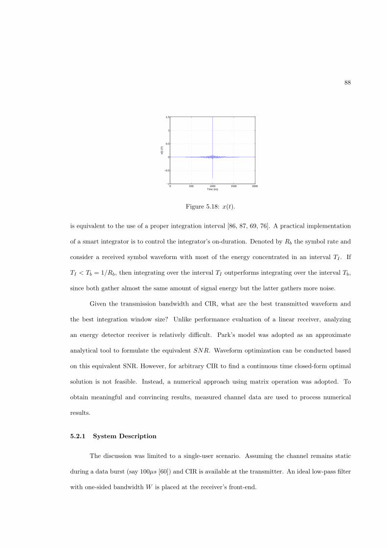
88
0 500 1000 1500 2000−1
−0.5
0
0.5
1
1.5
Time (ns)
x(t)
(V
)
Figure 5.18: x(t).
is equivalent to the use of a proper integration interval [86, 87, 69, 76]. A practical implementation
of a smart integrator is to control the integrator’s on-duration. Denoted by Rb the symbol rate and
consider a received symbol waveform with most of the energy concentrated in an interval TI . If
TI < Tb = 1/Rb, then integrating over the interval TI outperforms integrating over the interval Tb,
since both gather almost the same amount of signal energy but the latter gathers more noise.
Given the transmission bandwidth and CIR, what are the best transmitted waveform and
the best integration window size? Unlike performance evaluation of a linear receiver, analyzing
an energy detector receiver is relatively difficult. Park’s model was adopted as an approximate
analytical tool to formulate the equivalent SNR. Waveform optimization can be conducted based
on this equivalent SNR. However, for arbitrary CIR to find a continuous time closed-form optimal
solution is not feasible. Instead, a numerical approach using matrix operation was adopted. To
obtain meaningful and convincing results, measured channel data are used to process numerical
results.
5.2.1 System Description
The discussion was limited to a single-user scenario. Assuming the channel remains static
during a data burst (say 100µs [60]) and CIR is available at the transmitter. An ideal low-pass filter
with one-sided bandwidth W is placed at the receiver’s front-end.
89
The transmitted signal with OOK modulation is given by
s(t) =
∞∑
j=−∞
djp(t − jTb), (5.38)
where Tb is the symbol duration,
p(t) is the transmitted symbol waveform defined over [0, Tp], and
dj ∈ {0, 1} is j-th transmitted bit.
Without loss of generality, assume the minimal propagation delay is equal to zero. The energy
of p(t) is normalized and defined as Eb,
∫ Tp
0
p2 (t) dt = 1 (5.39)
The received noise-polluted signal at the output of the receiver front-end filter is given by
r(t) = h(t) ⊗ s(t) + n(t)
=
∞∑
j=−∞
djx(t − jTb) + n(t), (5.40)
where h (t) , t ∈ [0, Th] is the multipath impulse response that takes into account the effect of
the RF front-end including the transceiver antennas.
“⊗” denotes convolution operation.
n(t) is a low-pass additive zero-mean Gaussian noise with one-sided bandwidth W and one-
sided power spectral density N0, and
x(t) is the received noiseless symbol-“1” waveform defined as
x(t) = h(t) ⊗ p(t). (5.41)
It was further assumed that Tb ≥ Th + Tp
def= Tx, i.e. no existence of ISI.
90
An energy detector receiver performs squaring operation, integration over a given time win-
dow TI , and threshold decision. Corresponding to the time index k, the k-th decision variable at
the output of the integrator is given by
zk =
∫ kTb+TI0+TI
kTb+TI0
r2(t)dt (5.42)
=
∫ kTb+TI0+TI
kTb+TI0
(dkx(t − kTb) + n(t))2dt (5.43)
where TI0 is the starting time of integration for each symbol and 0 ≤ TI0 < TI0 + TI ≤ Tx ≤
Tb.
5.2.2 Waveform Design
5.2.2.1 Equivalent SNR. Analyzing an energy detector receiver as shown in Figure 5.19
is not as easy as analyzing linear receiver. The decision statistic zk can be approximated as a chi-
square or a non-central chi-square random variable, with 2TW degrees of freedom [88, 89]. A number
of approximating models have been proposed to evaluate the performance of receiver operating
characteristic (RCO) [90]. When 2TW is large, the chi-square or a non-central chi-square pdfs
asymptotically become Gaussian by the central limit theorem. In this case, the required receive
SNR and decision threshold can be determined, given the probability of false alarm Pf and the
probability of detection Pd [90]. With the notation used in this paper, the received SNR before the
square law is expressed as
dI =
∫ TI0+TI
TI0
x2 (t) dt
TIWN0(5.44)
The ROC formulas based on Gaussian approximation can be extended to handle arbitrary
value of 2TW by introducing an empirical loss function C(dI) [91, 92], with its general form
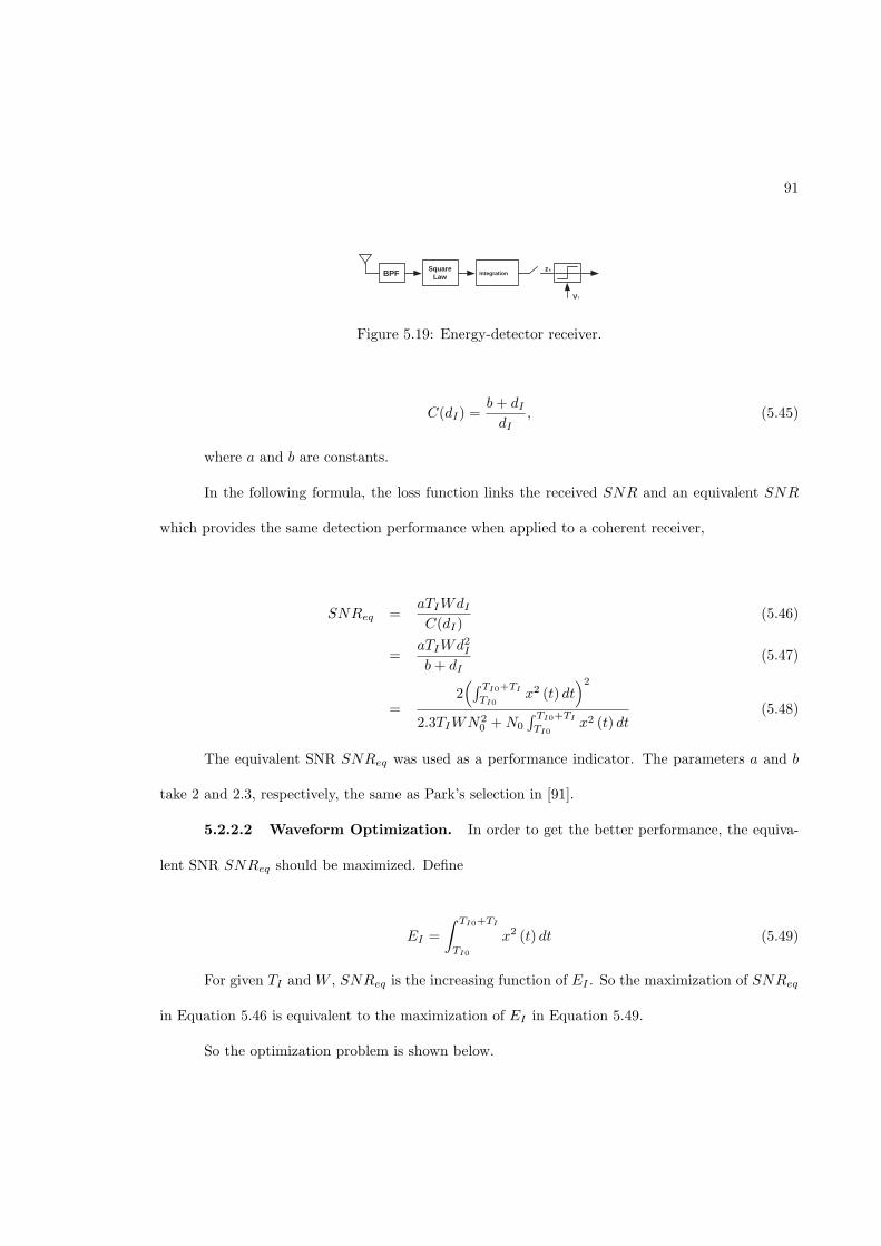
91
BPF z k
Integration
V T
Square Law
Figure 5.19: Energy-detector receiver.
C(dI) =b + dI
dI
, (5.45)
where a and b are constants.
In the following formula, the loss function links the received SNR and an equivalent SNR
which provides the same detection performance when applied to a coherent receiver,
SNReq =aTIWdI
C(dI)(5.46)
=aTIWd2
I
b + dI
(5.47)
=2(
∫ TI0+TI
TI0
x2 (t) dt)2
2.3TIWN20 + N0
∫ TI0+TI
TI0
x2 (t) dt(5.48)
The equivalent SNR SNReq was used as a performance indicator. The parameters a and b
take 2 and 2.3, respectively, the same as Park’s selection in [91].
5.2.2.2 Waveform Optimization. In order to get the better performance, the equiva-
lent SNR SNReq should be maximized. Define
EI =
∫ TI0+TI
TI0
x2 (t) dt (5.49)
For given TI and W , SNReq is the increasing function of EI . So the maximization of SNReq
in Equation 5.46 is equivalent to the maximization of EI in Equation 5.49.
So the optimization problem is shown below.
92
max∫ TI0+TI
TI0
x2 (t) dt
s.t.∫ Tp
0p2 (t) dt = 1
(5.50)
In order to solve the optimization problem 5.50, p(t), h(t), and x(t) will be uniformly sampled
and the count-part of the optimization problem 5.50 in the digital domain will be solved. Assume
the sampling period is Ts. Tp/Ts = Np, Th/Ts = Nh and Tx/Ts = Nx. So Nx = Np + Nh.
p(t), h(t) and x(t) are represented by pi, i = 0, 1, . . . , Np, hi, i = 0, 1, . . . , Nh and xi, i =
0, 1, . . . , Nx, respectively, where
pi = p (its) (5.51)
hi = h (its) (5.52)
xi = x (its) (5.53)
So the count-part of Equation 5.41 in the digital domain is shown as
xi = pi ∗ hi (5.54)
=
Np∑
j=0
pjhi−j (5.55)
Define
p = [p0 p1 · · · pNp]T (5.56)
and
x = [x0 x1 · · · xNx]T (5.57)
93
Construct channel matrix H(Nx+1)×(Np+1),
(H)i,j =
hi−j , 0 ≤ i − j ≤ Nh
0, else
(5.58)
where (•)i,j denotes the entry in the i-th row and j-th column of the matrix.
Thus the matrix expression of Equation 5.54 is
x = Hp (5.59)
and the constraint in the optimization problem 5.50 can be expressed as
‖p‖22 Ts = 1 (5.60)
where “‖•‖2” denotes the norm-2 of the vector.
Meanwhile assume TI/Ts = NI and TI0/Ts = NI0, so the valid entries in x for integration
constitute xI as
xI = [xNI0xNI0+1 · · · xNI0+NI
]T (5.61)
and EI in Equation 5.49 can be equivalently shown as
EI = ‖xI‖22 Ts (5.62)
Similar to Equation 5.59, xI can be obtained by
xI = HIp (5.63)
where (HI)i,j = (H)NI0+i,j and i = 1, 2, . . . , NI + 1 as well as j = 1, 2, . . . , Np + 1.
So the count-part of the optimization problem 5.50 in the digital domain can be expressed as
94
max EI
s.t. ‖p‖22 Ts = 1
(5.64)
Define
J = EI + λ(
1 − ‖p‖22 Ts
)
(5.65)
= ‖HIp‖22 Ts + λ
(
1 − ‖p‖22 Ts
)
(5.66)
where λ is Lagrange Multiplier. From ∂J∂p
= 0, it is obtained that
HTI HIp = λp (5.67)
So take the eigen-vector p∗ corresponding to the maximum eigen-value in eigen-function 5.67
as the candidate waveform. Meanwhile p∗ satisfies Equation 5.60. Furthermore, E∗
I will be obtained.
5.2.3 Channel Sounding
The time domain channel sounding is employed to get h(t). This kind of channel sounding
consists of a pulse generator, a signal generator, a low noise amplifier (LNA), a transmitter an-
tenna and a receiver antenna, and a digital sampling oscilloscope (DSO). Figure 5.20 shows the
setup of the time domain channel sounding. The signal generator, the pulse generator, and the
transmitter antenna constitute the transmitter part and DSO along with the receiver antenna and
LNA constitutes the receiver part. The signal generator is used to trigger the pulse generator and
the pulse generator generates the pulse that is transmitted through the channel. On the receiver
side the signal is amplified by LNA and then displayed and recorded on DSO. A triggering signal
from the signal generator is also used to synchronize DSO to record the data of the received signal.
The tapped-delay-line model of CIR will be estimated using ‘CLEAN’, a matching pursuit algorithm
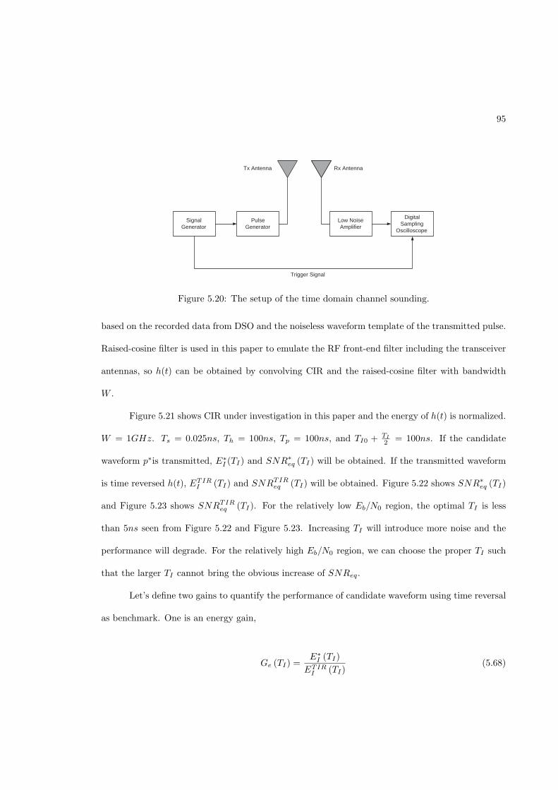
95
Signal Generator
Pulse Generator
Low Noise Amplifier
Digital Sampling
Oscilloscope
Tx Antenna Rx Antenna
Trigger Signal
Figure 5.20: The setup of the time domain channel sounding.
based on the recorded data from DSO and the noiseless waveform template of the transmitted pulse.
Raised-cosine filter is used in this paper to emulate the RF front-end filter including the transceiver
antennas, so h(t) can be obtained by convolving CIR and the raised-cosine filter with bandwidth
W .
Figure 5.21 shows CIR under investigation in this paper and the energy of h(t) is normalized.
W = 1GHz. Ts = 0.025ns, Th = 100ns, Tp = 100ns, and TI0 + TI
2 = 100ns. If the candidate
waveform p∗is transmitted, E∗
I (TI) and SNR∗
eq (TI) will be obtained. If the transmitted waveform
is time reversed h(t), ETIRI (TI) and SNRTIR
eq (TI) will be obtained. Figure 5.22 shows SNR∗
eq (TI)
and Figure 5.23 shows SNRTIReq (TI). For the relatively low Eb/N0 region, the optimal TI is less
than 5ns seen from Figure 5.22 and Figure 5.23. Increasing TI will introduce more noise and the
performance will degrade. For the relatively high Eb/N0 region, we can choose the proper TI such
that the larger TI cannot bring the obvious increase of SNReq.
Let’s define two gains to quantify the performance of candidate waveform using time reversal
as benchmark. One is an energy gain,
Ge (TI) =E∗
I (TI)
ETIRI (TI)
(5.68)
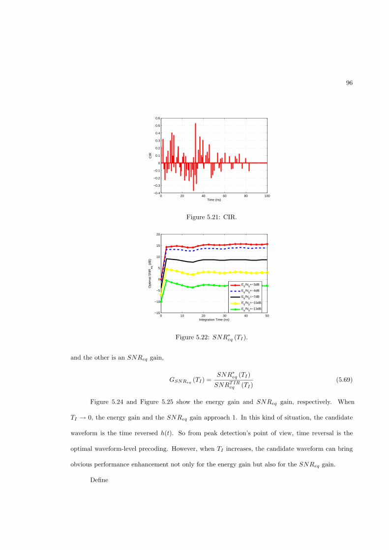
96
0 20 40 60 80 100−0.4
−0.3
−0.2
−0.1
0
0.1
0.2
0.3
0.4
0.5
0.6
Time (ns)
CIR
Figure 5.21: CIR.
0 10 20 30 40 50−15
−10
−5
0
5
10
15
20
Integration Time (ns)
Opt
imal
SN
Req
(dB
)
Eb/N
0=−3dB
Eb/N
0=−4dB
Eb/N
0=−7dB
Eb/N
0=−10dB
Eb/N
0=−13dB
Figure 5.22: SNR∗
eq (TI).
and the other is an SNReq gain,
GSNReq(TI) =
SNR∗
eq (TI)
SNRTIReq (TI)
(5.69)
eq
TI → 0, the energy gain and the SNReq gain approach 1. In this kind of situation, the candidate
waveform is the time reversed h(t). So from peak detection’s point of view, time reversal is the
optimal waveform-level precoding. However, when TI increases, the candidate waveform can bring
obvious performance enhancement not only for the energy gain but also for the SNReq gain.
Define
Figure 5.24 and Figure 5.25 show the energy gain and SNR gain, respectively. When
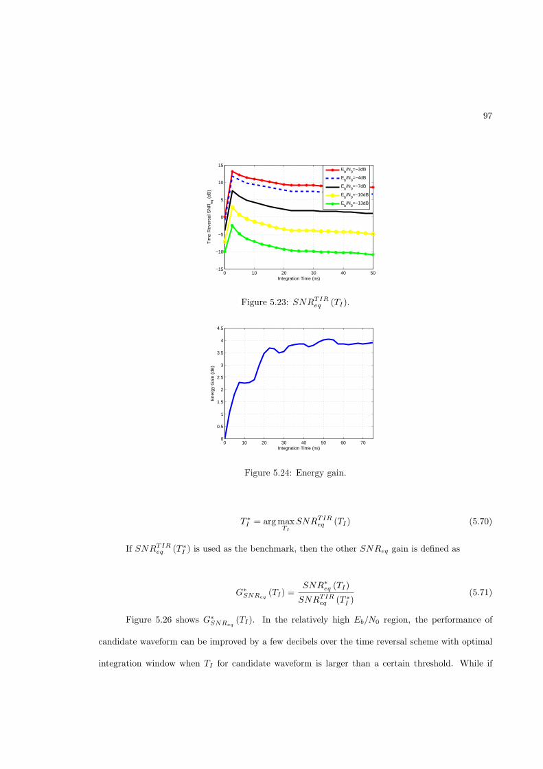
97
0 10 20 30 40 50−15
−10
−5
0
5
10
15
Integration Time (ns)
Tim
e R
ever
sal S
NR
eq (
dB)
E
b/N
0=−3dB
Eb/N
0=−4dB
Eb/N
0=−7dB
Eb/N
0=−10dB
Eb/N
0=−13dB
Figure 5.23: SNRTIReq (TI).
0 10 20 30 40 50 60 700
0.5
1
1.5
2
2.5
3
3.5
4
4.5
Integration Time (ns)
Ene
rgy
Gai
n (d
B)
Figure 5.24: Energy gain.
T ∗
I = arg maxTI
SNRTIReq (TI) (5.70)
If SNRTIReq (T ∗
I ) is used as the benchmark, then the other SNReq gain is defined as
G∗
SNReq(TI) =
SNR∗
eq (TI)
SNRTIReq (T ∗
I )(5.71)
Figure 5.26 shows G∗
SNReq(TI). In the relatively high Eb/N0 region, the performance of
candidate waveform can be improved by a few decibels over the time reversal scheme with optimal
integration window when TI for candidate waveform is larger than a certain threshold. While if
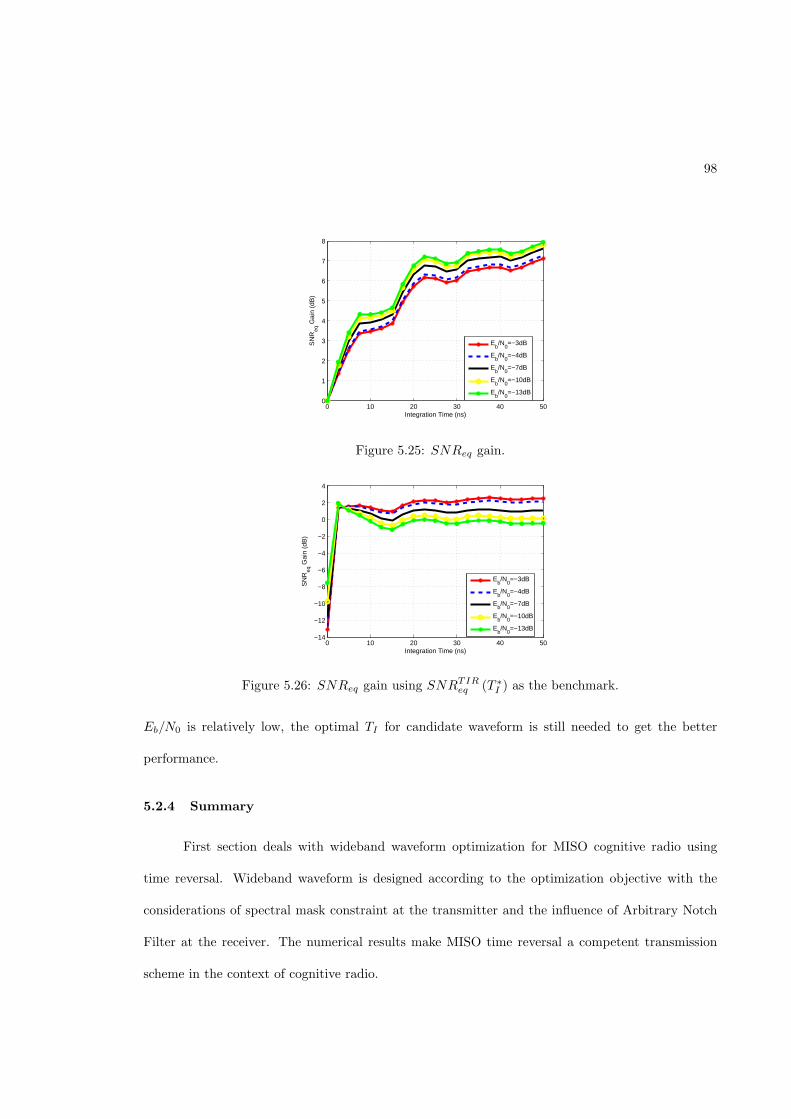
98
0 10 20 30 40 500
1
2
3
4
5
6
7
8
Integration Time (ns)
SN
Req
Gai
n (d
B)
Eb/N
0=−3dB
Eb/N
0=−4dB
Eb/N
0=−7dB
Eb/N
0=−10dB
Eb/N
0=−13dB
Figure 5.25: SNReq gain.
0 10 20 30 40 50−14
−12
−10
−8
−6
−4
−2
0
2
4
Integration Time (ns)
SN
Req
Gai
n (d
B)
Eb/N
0=−3dB
Eb/N
0=−4dB
Eb/N
0=−7dB
Eb/N
0=−10dB
Eb/N
0=−13dB
Figure 5.26: SNReq gain using SNRTIReq (T ∗
I ) as the benchmark.
Eb/N0 is relatively low, the optimal TI for candidate waveform is still needed to get the better
performance.
5.2.4 Summary
First section deals with wideband waveform optimization for MISO cognitive radio using
time reversal. Wideband waveform is designed according to the optimization objective with the
considerations of spectral mask constraint at the transmitter and the influence of Arbitrary Notch
Filter at the receiver. The numerical results make MISO time reversal a competent transmission
scheme in the context of cognitive radio.
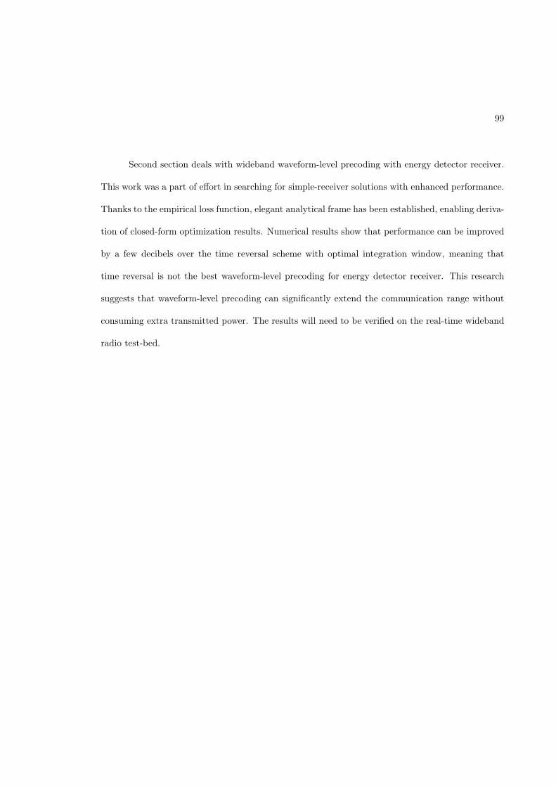
99
Second section deals with wideband waveform-level precoding with energy detector receiver.
This work was a part of effort in searching for simple-receiver solutions with enhanced performance.
Thanks to the empirical loss function, elegant analytical frame has been established, enabling deriva-
tion of closed-form optimization results. Numerical results show that performance can be improved
by a few decibels over the time reversal scheme with optimal integration window, meaning that
time reversal is not the best waveform-level precoding for energy detector receiver. This research
suggests that waveform-level precoding can significantly extend the communication range without
consuming extra transmitted power. The results will need to be verified on the real-time wideband
radio test-bed.
CHAPTER 6
CONCLUSION AND FUTURE WORK
6.1 Conclusion
An automation was provided to operate the systems for spectrum occupancy and channel
sounding more precisely. LabVIEW 8.5 was used as a tool to control spectrum analyzer, vector
network analyzer, and digital sampling oscilloscope from a remote terminal. GPIB protocol of the
instruments under investigation was used remote communication with LabVIEW computer/laptop,
using USB-2 protocol on remote computer.
Spectrum occupancy measurements were performed for the CDMA, GSM, Wi-Fi, and DTV
signals and 3-D plots were obtained using MatLAB to process the acquired data. These plots enable
us to learn the statistics of spectrum under investigation. The acquired data serves as a raw data for
the efficient development of cognitive radio/cognitive radar. Since, as per IEEE802.22 and FCC’s
rulings the TV band is primary guy to work on for the cognitive radio, thus a detailed measurement
for DTV spectrum was presented in this approach. It was clearly mentioned that a DTV signal is
a strong candidate around 50 Km to 60 Km range area from a TV transmitting antenna. But after
that, the signal strength really depends on the geographical environment. From this, it could also
be concluded that between the range of a particular TV transmitter, only 6 MHz frequency band,
in which the TV station is broadcasting, is used e.g. as discussed here, that WCTE had a 6 MHz
channels ranging from Channel-2 to Channel-69(exclude Ch-22 from this) are free to use by the
secondary users in this vicinity.
Frequency domain and time domain channel sounding was performed in metal confined, office,
and hallway locations. The frequency domain and time domain results were presented as a 3-D plots
100
allocated frequency band with 521 MHz (Ch-22) as a center frequency, whereas all other allocated
101
obtained using MatLAB to process the acquired data. Automated system enables us to perform
fast data acquisition and accurate channel sounding. A novel approach was shown to do wideband
waveform optimization using MISO case and by using VNA to get the frequency domain data. The
work was further extended to do waveform-level precoding, using DSO to collect the time domain
data. Reconstructing the spectral trace for quickest detection was also performed in this work.
6.2 Future Work
Since all the key instruments are now automated, the key area to work in near future is to
add a automated mobility at transmitter or receiver antenna side, so that the statistical modeling
of channel behavior could be performed, assuming a moving target inside metal cavity, office envi-
ronment, or hallway environment. The other future work may include to use spectrum data as a
key ingredient, to develop algorithms which can deal with automatic decision making more simple.

BIBLIOGRAPHY
102
103
[1] Cabric, D., Mishra, S.M., and Brodersen, R.W. “Implementation Issues in Spectrum Sensingfor Cognitive Radios.” In “Signals, Systems and Computers, 2004. Conference Record of theThirty-Eighth Asilomar Conference on,” volume 1, pages 772–776, 2004.
[2] Akyildiz, IF, Lee, W.Y., Vuran, MC, and Mohanty, S. “A survey on spectrum managementin cognitive radio networks [cognitive radio communications and networks].” CommunicationsMagazine, IEEE , volume 46, no. 4, pages 40–48, 2008.
[3] Sherman, M., Mody, A. N., Martinez, R., Rodriguez, C., and Reddy, R. “IEEE StandardsSupporting Cognitive Radio and Networks, Dynamic Spectrum Access, and Coexistence.” IEEECommunications Magazine, pages 72–79, July 2008.
[4] Haykin, S. “Cognitive Radar.” IEEE SIGNAL PROCESSING MAGAZINE , pages 30–40, Jan.2006.
[5] Nehorai, A., Gini, F., Greco, M. S., Panpandreou-Suppappola, A., and Rangaswamy, M. “In-troduction to the Issue on Adaptive Waveform Design for Agile Sensing and Communication.”IEEE J. Selet. Topics Signal Proc., volume 1, no. 1, pages 2–5, June 2007. Editorial for SpecialIssue.
[6] Qiu, R. C., Liu, H. P., and Shen, X. “Ultra-Wideband for Multiple Access.” CommunicationsMagazine, pages 2–9, Feb. 2005.
[7] Cabric, D. “Spectrum Sharing Radios.” IEEE Circuits and Systems Magazine, volume 6, no. 2,pages 30–45, 2006.
[8] Mitola III, J. Cognitive Radio Architecture. John Wiley, 2006.
[9] Kim, K. Exploiting Cyclostationarity for Radio Environmental Awareness in Cognitive Radios.Ph.D. thesis, Virginia Polytechnic Institute and State University, 2008.
[10] Challapali, K., Cordeiro, C., and Birru, D. “Evolution of Spectrum-Agile Cognitive Radio:First Wireless Internet Standard and Beyond.” WiCON 2006, August 2007.
[11] Qiu, R., Guo, N., Li, H., Wu, Z., Chakravarthy, V., Song, Y., Hu, Z., Zhang, P., and Chen, Z.“A Unified Framework for Cognitive Radio, Cognitive Radar, and Electronic WarfareTutorial,Theory, and Multi-GHz Wideband Testbed.” Sensors, 2009.
[12] Shewhart, W. A. Economic Control of Manufactured Products. Van Nostrand Reinhold, NewYork, 1931.
[13] Marcus, M. and Swerling, P. “Sequential detection in radar with multiple resolution elements.”IEEE Trans. Inform. Theory , volume 8, pages 237–242, 1963.
[14] V. F. Pisarenko, A. F. Kushnir and Savin, I. V. “Statistical adaptive algorithms for estimationof onset moments of seismic plates.” Physics of the Earth and Planetary Interiors, volume 47,pages 4–10, 1987.
[15] Coppin, P. R. and Bauer, M. E. “Change detection in forest ecosystems with remote sensingdigital imagery.” Remote Sensing Reviews , volume 13, pages 207–234, 1996.
[16] Basseville, M. “Edge detection using sequential methods for change in level - Part II: Sequentialdetection of a change in mean.” IEEE Trans. Acoust. Speech. Signal Processing , volume 29,pages 29–40, Jan 1981.
104
[17] Jaruskova, D. “Some problems with application of change-point detection methods to environ-mental data.” EnvironMetrics, volume 8, pages 469–483, May 1997.
[18] Pettersson, M. “Monitoring a freshwater fish population: Statistical surveillance of biodiver-sity.” EnvironMetrics, volume 9, pages 139–150, Feb. 1998.
[19] M. C. Yang, R. G. Marks I. Magnusson, Y. Y. Namgung and Clark, W. B. “Change detectionon longitudinal data in periodontal research.” Journal of Periodontal Research, volume 28,pages 152–160, 1993.
[20] T. Friede, W. Bischoff, F. Miller and Kieserc, M. “A note on change point estimation indose-response trials.” Computational Statistics and Data Analysis, volume 37, pages 219–232,2001.
[21] M. Petzold, E. Bergman, C. Sonesson and Kieler, H. “Surveillance in longitudinal models:Detection of intrauterine growth restriction.” Biometrics, volume 60, pages 1025–1033, 2004.
[22] Y. Mei, L. Wang and Holte, S. E. “A comparison of methods for determining HIV viral setpoint.” Statistics in Medecine, July 2007.
[23] Andre-Obrecht, R. “A new statistical approach for the automatic segmentation of continousspeech signals.” IEEE Trans. Acoust. Speech. Signal Processing , volume 36, pages 29–40, Jan1988.
[24] Lelescu, D. and Schonfeld, D. “Statistical sequential analysis for real-time video scene changedetection on compressed multimedia bitstream.” IEEE Trans. Multimedia, volume 5, pages106–117, Jan. 2005.
[25] M. K. Omar, U. Chaudhari and Ramaswamy, G. N. “Blind change detection for audio segmen-tation.” In “Proceedings of ICASSP,” Philadelphia, PA, March 2005.
[26] Papantoni-Kazakos, P. “Algorithms for monitoring changes in quality of communication links.”IEEE Trans. Commun., volume 27, pages 682–693, April 1976.
[27] Chang, R. K. C. “Defending against flooding-based distributed denial-of-service attacks: Atutorial.” IEEE Communications Magazine, volume 40, pages 42–51, Oct. 2002.
[28] Thottan, M. and Ji, C. “Anomaly detection in IP networks.” IEEE Trans. Signal Processing ,volume 51, pages 2191–2204, Aug 2003.
[29] J. S. Baras, A. Cardenas and Ramezani, V. “Distributed change detection for worms, ddos andother network attacks.” In “Proceedings of the 2004 American Control Conference,” Boston,MA,, 2004.
[30] A. Tartakovsky, R. Blazek, B. Rozovskii and Kim, H. “A novel approach to detection of intru-sions in computer networks via adaptive sequential and batch-sequential change-point detectionmethods.” IEEE Trans. Signal Processing , volume 54, pages 3372–3382, 2006.
[31] S. Radosavac, J. S. Baras, A. A. Cardenas and Moustakides, G. V. “Detecting IEEE 802.11MAC layer mibehavior in ad hoc networks: Robust strategies against individual and colludingattackers.” Journal of Computer Security , volume 15, pages 103–128, 2007.
[32] Tartakovsky, A. and Veeravalli, V. V. “Quickest change detection in distributed sensor net-works.” Proceedings of the 6th International Conference on Information Fusion, 2003.
105
[33] Moustakides, G. V. “Decentralized CUSUM change detection.” In “Proceedings of 9th Inter-national Conference on Information Fusion,” Florence, Italy,, 2006.
[34] Veeravalli, V. V. “Quickest change detection in sensor networks.” In “First InternationalWorkshop in Sequential Methodologies (IWSM),” Auburn, AL, 2007.
[35] Basseville, M. and Nikiforov, I. Detection of Abrupt Changes:Theory and Applications. Prentice-Hall,Englewood Cliffs, 1993.
[36] Poor, H. V. Quickest Detection. Cambridge, UK: Cambridge University Press, 2008.
[37] X., Shen, M., Guizani, R. C., Qiu, and T., Le-Ngoc. UWB Wireless Communications andNetworks. Wiley, 2006.
[38] Ghavami, M., Michael, LB, and Kohno, R. Ultra wideband signals and systems in communica-tion engineering . Wiley, 2004.
[39] Oppermann, I. and Iinatti, J. UWB Theory and Applications. Wiley, 2004.
[40] National Instruments. http://zone.ni.com/reference/en-XX/help/371361D-01/TOC10.htm.
[41] National Instruments. http://zone.ni.com/reference/en-XX/help/371361D-01/ .
[42] Marcus, M., Burtle, J., Franca, B., Lahjouji, A., and McNeil, N. “Federal CommunicationsCommission Spectrum Policy Task Force.” In “Report of the Unlicensed Devices and Experi-mental Licenses Working Group,” , November 2002.
[43] http://news.cnet.com/8301-1035 3-10082505-94.html .
[44] Petty, V.R. “A Framework for Radio Frequency Spectrum Measurement and Analysis.” Tech-nical Report ITTC-FY2008-TR-34330-02, The University of Kansas, Information & Telecom-munication Technology Center, March 2008.
[45] McHenry, M.A. “NSF Spectrum Occupancy Measurements Project Summary.” Technicalreport, Shared Spectrum Company, August 2005.
[46] Spectrum Planning Subcommittee, Working Group 7. “Federal LongRange Spectrum Plan.”In “Federal LongRange Spectrum Plan,” National Telecommunications and Information Ad-ministration, 2000.
[47] Qiu, Robert, Guo, Nan, Yu, Song, Hu, Zhen, Zhang, Peng, Saini, Amanpreet, Chen, Zhe, andCurrie, Kenneth. “Towards An Integration of Wideband (Multi-GHz) Cognitive Radio andCognitive Radar: Testbed and Architecture.”, November 2008. DSA Workshop Presentation,Dayton, Ohio.
[48] Test and Division, Measurement. Operating Manual: SPECTRUM ANALYZER (Vol-I). Rohdeand Schwarz, volume 1 edition.
[49] Test and Division, Measurement. Operating Manual: SPECTRUM ANALYZER (Vol-II). Ro-hde and Schwarz, volume 2 edition.
[50] http://www.stanford.edu/ boyd/cvx/ .
[51] Boyd, Stephen and Vandenberghe, Lieven. Convex Optimization. Press Syndicate of the Uni-versity of Cambridge, 2004.
106
[52] Agilent Technologies, www.agilent.com/find/assist. Understanding the Fundamental Principlesof Vector Network Analysis. Application Note.
[53] Pierce, J.R. and Hopper, A.L. “Nonsynchrous Time Division Withholding and With RandomSampling.” In “Proc. IRE,” pages 1079–1088, September 1952.
[54] Rushforth, C.K. “Transmitted-reference Techniques for Random or Unknown Channel.” IEEETrans. on Information Theory , volume 10, no. 1, pages 39–42, January 1964.
[55] Hingorani, G. and Hancock, J. “A Transmitted Reference System for Communication in Ran-dom of Unknown Channels.” IEEE Transactions on Communications Technology , volume 13,no. 3, pages 293–301, 1965.
[56] van Stralen, N., Dentinger, A., Welles, K., Gauss, R., Hoctor, R., and Tomlinson, H. “DelayHopped Transmitted Reference Experimental Results.” In “IEEE Conference on Ultra Wide-band Systems and Technologies,” pages 93–98, 2002.
[57] Choi, J.D. and Stark, W.E. “Performance of Ultra-Wideband Communications with Subopti-mal Receivers in Multipath Channels.” IEEE Journal on Selected Areas in Communications,volume 20, no. 9, pages 1754–1766, 2002.
[58] Goeckel, D.L. and Zhang, Q. “Slightly Frequency-shifted Transmitted-reference UltrawidebandRadio: TR-UWB without the Delay Element.” In “IEEE MILCOM,” , October 2005.
[59] Goeckel, D.L., Mehlman, J., and Burkhart, J. “A Class of Ultra Wideband (UWB) Systemswith Simple Receivers.” In “IEEE Military Communications Conference,” pages 1–7, 2007.
[60] Liu, H., Molisch, A.F., Zhao, S., Goeckel, D., and Orlik, P. “Hybrid Coherent and Frequency-Shifted-Reference Ultrawideband Radio.” In “IEEE Global Telecommunications Conference,”pages 4106–4111, 2007.
[61] Ho, M., Somayazulu, VS.., Foerster, J., and Roy, S. “A Differential Detector for an Ultra-wideband Communications System.” IEEE 55th Vehicular Technology Conference, volume 4,pages 1896–1900, 2002.
[62] Chao, Y.L. and Scholtz, R.A. “Optimal and Suboptimal Receivers for Ultra-wideband Trans-mitted Reference Systems.” In “IEEE Global Telecommunications Conference,” volume 2,pages 759–763, 2003.
[63] Zhao, S., Liu, H., and Tian, Z. “A Decision-Feedback Autocorrelation Receiver for PulsedUltra-wideband Systems.” In “IEEE Radio and Wireless Conference,” pages 251–254, 2004.
[64] Guo, N. and Qiu, R. C. “Improved Autocorrelation Demodulation Receivers Based on Multiple-symbol Detection for UWB Communications.” IEEE Trans. Wireless Communications, vol-ume 5, no. 8, pages 2026–2031, 2006.
[65] V., Lottici and Z., Tian. “Multiple Symbol Differential Detection for UWB communications.”IEEE Trans. Wireless Commun., volume 7, pages 1656–1666, 2008.
[66] Souilmi, Y. and Knopp, R. “On the Achievable Rates of Ultra-wideband PPM with Non-Coherent Detection in Multipath Environments.” In “IEEE International Conference on Com-munications,” volume 5, pages 3530–3534, 2003.
107
[67] Weisenhorn, M. and Hirt, W. “Robust Noncoherent Receiver Exploiting UWB Channel Prop-erties.” In “Proc. IEEE Joint UWBST & IWUWBS,” pages 156–160, 2004.
[68] Paquelet, S., Aubert, L.M., Uguen, B., Mitsubishi, I.T.E.T.C.L., and Rennes, F. “An ImpulseRadio Asynchronous Transceiver for High Data rates.” In “International Workshop on UltraWideband Systems, Joint with Conference on Ultrawideband Systems and Technologies,” pages1–5, 2004.
[69] Guo, N., Zhang, J.Q., Qiu, R.C., and Mo, S. “UWB MISO Time Reversal With Energy Detec-tor Receiver Over ISI Channels.” In “4th IEEE Consumer Communications and NetworkingConference,” pages 629–633, 2007.
[70] Guo, N., Qiu, R. C., Zhang, Q., Sadler, B. M., Hu, Z., Zhang, P., Song, Y., and Zhou, C. M.Handbook of Sensor Networks , chapter Time Reversal for Ultra-Wideband Communications:Architecture and Test-bed, pages 1–41. World Scientific Publishing, 2009.
[71] Fink, M. “Time-reversal of Ultrasonic Fields—Part I: Basic Principles.” IEEE Trans. Ultrason.Ferroelec. Freq. Control , volume 39, no. 5, pages 555–566, 1992.
[72] Akogun, A. E., Qiu, R. C., and Guo, N. “Demonstrating Time Reversal in Ultra-WidebandCommunications using Time Domain Measurements.” pages 8–12, May 2005.
[73] Guo, N., Qiu, R. C., and Sadler, B. M. “An Ultra-Wideband Autocorrelation DemodulationScheme with Low-Complexity Time Reversal Enhancement.” In “IEEE Military Communica-tions Conference,” volume 5, pages 3066–3072, October 2005.
[74] Qiu, R. C., Zhou, C., Guo, N., and Zhang, J. Q. “Time Reversal with MISO for Ultra-Wideband Communications: Experimental Results (invited paper).” In “IEEE Radio andWireless Symposium,” San Diego, CA, 2006.
[75] Guo, N., Zhang, J.Q., Qiu, R.C., and Mo, S. “UWB MISO Time Reversal With EnergyDetector Receiver Over ISI Channels.” In “IEEE Consumer Commun. and Networking Conf,”pages 11–13, 2007.
[76] Guo, N., Qiu, R. C., and Sadler, B. M. “Reduced-Complexity Time Reversal Enhanced Auto-correlation Receivers Considering Experiment-Based UWB Channels.” IEEE Trans. WirelessComm., volume 6, no. 12, 2007.
[77] Witrisal, K., Leus, G., Pausini, M., and Krall, C. “Equivalent System Model and Equalizationof Differential Impulse Radio UWB Systems.” IEEE Journal on Selected Areas in Communi-cations, volume 23, no. 9, pages 1851–1862, 2005.
[78] Pausini, M., Janssen, G.J.M., and Witrisal, K. “Performance Enhancement of Differential UWBAutocorrelation Receivers Under ISI.” IEEE Journal on Selected Areas in Communications,volume 24, no. 4 Part 1, pages 815–821, 2006.
[79] Wilson, R., Tse, D., and Scholtz, R.A. “Channel Identification: Secret Sharing Using Reci-procity in Ultrawideband Channels.” IEEE Transactions on Information Forensics and Secu-rity , volume 2, no. 3 Part 1, pages 364–375, 2007.
[80] Bloch, M., Barros, J., Rodrigues, M.R.D., and McLaughlin, S.W. “Wireless Information-Theoretic Security.” IEEE Transactions on Information Theory , volume 54, no. 6, pages 2515–2534, 2008.
108
[81] Romme, J., Durisi, G., GmbH, I., and Kamp-Lintfort, G. “Transmit Reference Impulse RadioSystems using Weighted Correlation.” In “International Workshop on Ultra Wideband Systems,Joint with Conference on Ultrawideband Systems and Technologies,” pages 141–145, 2004.
[82] Chao, Y.L. and Scholtz, R.A. “Weighted Correlation Receivers for Ultra-Wideband TransmittedReference Systems.” In “IEEE Global Telecommunications Conference,” volume 1, pages 66–70,2004.
[83] Romme, J. and Witrisal, K. “Transmitted-Reference UWB Systems Using Weighted Auto-correlation Receivers.” IEEE Transactions on Microwave Theory and Techniques, volume 54,no. 4, pages 1754–1761, 2006.
[84] Tian, Z. and Sadler, BM. “Weighted Energy Detection of Ultra-Wideband Signals.” In “IEEE6th Workshop on Signal Processing Advances in Wireless Communications,” pages 1068–1072,2005.
[85] Wu, J., Xiang, H., and Tian, Z. “Weighted Noncoherent Receivers for UWB PPM Signals.”IEEE COMMUNICATIONS LETTERS , volume 10, no. 9, page 655, 2006.
[86] Franz, S. and Mitra, U. “Integration Interval Optimization and Performance Analysis for UWBTransmitted Reference Systems.” In “International Workshop on Ultra Wideband Systems,Joint with Conference on Ultrawideband Systems and Technologies.”, pages 26–30, 2004.
[87] Chao, Y.L. “Optimal Integration Time for UWB Transmitted Reference Correlation Receivers.”In “Conference Record of the Thirty-Eighth Asilomar Conference on Signals, Systems andComputers,” volume 1, 2004.
[88] Urkowitz, H. “Energy Detection of unknown Deterministic Signals.” Proceedings of the IEEE ,volume 55, no. 4, pages 523–531, 1967.
[89] Torrieri, D.J. Principles of Secure Communication Systems. Artech House, Inc. Norwood, MA,USA, 1992.
[90] Mills, RF and Prescott, GE. “A Comparison of Various Radiometer Detection Models.” IEEETransactions on Aerospace and Electronic Systems, volume 32, no. 1, pages 467–473, 1996.
[91] Park, K.Y. “Performance Evaluation of Energy Detectors.” IEEE Transactions on Aerospaceand Electronic Systems, volume 14, pages 237–241, 1978.
[92] Barton, D.K. “Simple Procedures for Radar Detection Calculations.” IEEE Transactions onAerospace and Electronic Systems, volume 5, pages 837–846, 1969.
VITA
Amanpreet Singh Saini was born in Punjab(State) in India, on March 12, 1979. He obtained
his B.S. in Electronics and Communication Engineering from Punjab Technical University, Jalland-
har, India, in May, 2001. Until December, 2006, he worked as Technical Support Executive in
Mumbai-based multi-national company in India . He entered Tennessee Technological University in
January, 2007, and is a candidate for the Master’s Degree in Electrical Engineering. During his stay
at Tennessee Technological University, he worked closely with his faculty advisor Dr Robert C. Qiu.
His research was focused on one externally-funded project through the Office of Naval Research and
two externally-funded projects through National Science Foundation.
109