spectral decomposition of time- versus depth-migrated...

Spectral decomposition of time- vs. depth-migrated data

Tengfei Lin*, the University of Oklahoma; Zhonghong Wan, BGP Inc., CNPC; Bo Zhang, Shiguang Guo and Kurt

Marfurt, the University of Oklahoma; Yi Guo, China University of Petroleum

Summary

Spectral decomposition is a powerful analysis tool that has

been significant success in delineating channels, fans,

overbank deposits and other relative thin architectural

elements of clastic and carbonate depositional

environments. Because of its success in fluvial-deltaic and

basin floor turbidite-fan systems, most publications of

spectral decomposition have used time-migrated data.

Interpreting spectral components and spectral attributes

such as peak frequency on depth migrated data requires a

slightly different perspective. First, the results are

computed as cycles/km (or alternatively as cycles/1000 ft)

rather than as cycles/s or Hertz, with the dominant

wavenumber decreasing with increasing velocities at depth.

Second, interpreters resort to depth migration when there

are significant lateral velocity changes in the overburden

and/or steep dips. All present-day implementations

compute spectral components vertical trace by vertical

trace rather than perpendicular to the bedding plane, giving

rise to tuning and other anomalies at an apparent rather than

at a true frequency or wavenumber.

We illustrate the interpretational differences of spectral

decomposition between time- and depth-migrated data

through the use of a simple synthetic model and a modern

3D data volume. We show how one can approximately

compensate for reflector dip by normalizing each spectral

magnitude component by 1/cosθ, where θ is the volumetric

dip magnitude commonly computed in seismic attribute

analysis

Introduction

Seismic attributes have been applied to depth-migrated data

since their inception. Since the dominant wavelength

increases with increasing velocity which in turn increases

with depth, attributes such as coherence benefit by using

shorter vertical analysis windows in the shallow section and

longer vertical analysis windows in the deeper section.

Since most coherence implementations require a fixed

vertical analysis window, the interpreter simply runs the

algorithm using an appropriate window for each zone to be

analyzed. Curvature is naturally computed in the depth

domain, with most algorithms requiring a simple

conversion velocity for time-migrated data. For more

accurate results, the interpreter uses different conversion

velocities for different target depths, or simply converts the

entire volume to depth using well control. Both coherence

and curvature are structurally driven algorithms, with

coherence computed along structural dip and curvature

computed from structural dip.

In contrast, spectral decomposition is computed trace by

trace which implicitly ignores any dipping structure. One of

the most common uses of spectral decomposition is to

map shallow (e.g. Partyka et al., 1999; Peyton et al., 1998)

and deepwater (e.g. Bahorich et al., 2002) stratigraphic

features using a simple thin bed tuning model. Widess

(1973) used a wedge model and found maximum

constructive interference occurs when the wedge

thickness equals the tuning thickness (one-half of the two-

way travel-time period for time-migrated data or one-

quarter of the wavelength for the depth-migrated data).

Using this model, Laughlin et al. (2002) shows that deeper

channels are stronger at lower frequencies, while the

shallower flank of the channel has stronger amplitudes at

higher frequencies. Although this is the most common use

of spectral decomposition, spectral components are

currently the method of choice in estimating attenuation

(1/Q), pore-pressure prediction, and seismic unconformities,

as well as some implementations of seismic

chronostratigraphy.

Theory

Short-window Discrete Fourier Transform (SWDFT),

Continuous Wavelet Transforms, and Matching Pursuit

There are currently three algorithms used to generate

spectral components: short-window discrete Fourier

transforms (SWDFT), continuous wavelet transforms, and

matching pursuit. Leppard et al. (2010) find that matching

pursuit provides greater vertical resolution and less vertical

stratigraphic mixing than the other techniques. For this

reason, all our examples here will be generated using a

matching pursuit algorithm described by Liu and Marfurt

(2007). However, the concept of apparent vs. true

frequency is perhaps easiest to understand using the fixed

length analysis window used in the SWDFT. For time data,

the window will be in seconds, such that the spectral

components are measured in cycles/s or Hz. For depth data,

the window will be in kilometers, such that the spectral

components are measured in cycles/km. Significant care

must be made when loading the data into commercial

software, where the SEGY standard stores the sample

interval in microseconds. For everything to work correctly,

a depth sample interval of 10 m will need to be stored as

DOI http://dx.doi.org/10.1190/segam2013-1166.1© 2013 SEGSEG Houston 2013 Annual Meeting 384

Dow

nloa

ded

01/2

3/14

to 1

29.1

5.12

7.24

5. R

edis

trib

utio

n su

bjec

t to

SEG

lice

nse

or c

opyr

ight

; see

Ter

ms

of U

se a

t http

://lib

rary

.seg

.org

/

10000 “microkilometers”. If the units are not stored in this

manner, the numerical values of the data may appear to

be in fractions of a cycles/m. Many commercial software

packages will not operate for cycles/s (or cycles/km) that

fall beyond a reasonable numerical range of 1-250.

Once the data are loaded, the range of values will be

different. If the time domain data range between 8-120 Hz,

depth domain data will range between 2-30 cycles/km at a velocity of 4 km/s, such that anomalies will be shifted to

the lower “frequencies”.

Volumetric dip and its influence

If the dip angle is , and the real thickness hr, then the

apparent thickness (Figure 1). The tuning

frequency (and tuning wavenumber) will therefore decrease

with increasing values of θ. The shift to lower apparent

frequency is familiar to those who examine data before and

after time migration, where dipping events on unmigrated

stacked data with moderate apparent frequency “migrate”

laterally to steeper events with lower apparent frequency.

Figure 1. The percent change in apparent thickness ha/hr with

respect to dip magnitude, θ.

Most volumetric dip computations provide apparent dips

along the survey axes, and , which in turn define the

unit normal, a, (Figure 2 where

, (1)

, and (2)

, (3)

where is the dip magnitude and is the dip azimuth.

The first eigenvector of dip estimates of the gradient

structure tensor provides a direct estimate a. Other

workers compute instantaneous frequency, ω, and

wavenumbers, kx and ky, or use a semblance dip scan to

compute apparent dips p and q measured in s/m.

;

(4)

(5)

Figure 2. The definition of reflector dip. (After Marfurt, 2006).

If the earth can be approximated by a constant velocity, v,

the relationships between apparent time dips p and q, and

the apparent angle dips and , are

, (6)

, (7)

(8)

A synthetic example

DOI http://dx.doi.org/10.1190/segam2013-1166.1© 2013 SEGSEG Houston 2013 Annual Meeting Page 1385

Dow

nloa

ded

01/2

3/14

to 1

29.1

5.12

7.24

5. R

edis

trib

utio

n su

bjec

t to

SEG

lice

nse

or c

opyr

ight

; see

Ter

ms

of U

se a

t http

://lib

rary

.seg

.org

/

Figure 3. (a) A thin bed model showing layers components with (1)

flat dip (2) strong dip to the left, and (3) moderate dip to the right.

(b) The apparent (in blue) and real (in red) tuning frequency of the

layer. (c) Synthetic seismic data generated by prestack time

migration and stacking a suite of shot gathers. The deeper event is

a multiple. (d) The peak frequency of (c) computed using a

matching pursuit algorithm. Note the peak frequency (50Hz) in

the layer corresponds to the apparent frequency in (b).

In Figure 3a, the vertical thickness of the thin bed is 100

m; the tuning frequency should be 50 Hz considering

the velocity is 5000 m/s. The apparent thickness is

constant across the model when measured vertically (blue

curve in Figure 3b) such that spectral analysis results in a

constant value of fpeak 50 Hz rather than the variable peak

frequency given by the red curve in Figure 4b. Correcting

the apparent thickness by 1/cosθ gives the correct answer.

We generated a suite of shot gathers for the model shown

in Figure 3a, migrated them, and then stacked the result,

giving the vertical section shown in Figure 3c. We then

computed the peak frequency using a matching pursuit

spectral decomposition. Note the constant value of 50 Hz

through the variable thickness layer.

Real Data Example

The real data are from an oilfield of east China. There are

lots of fault-controlled reservoirs, exhibiting strongly on

the seismic profile shown on both the time migrated

and depth migrated data in Figure 4. The blue color

cover the same position in both profiles, we found that

the horizons are much deeper in depth migrated data

than the ones in time migrated data. This is because the

increase of velocity with time (depth).

The migrated data are sampled at Δt=0.002 s in time and

Δz=0.01 km in depth. Figure 5 shows the average spectra

of the data shown in Figure 4.

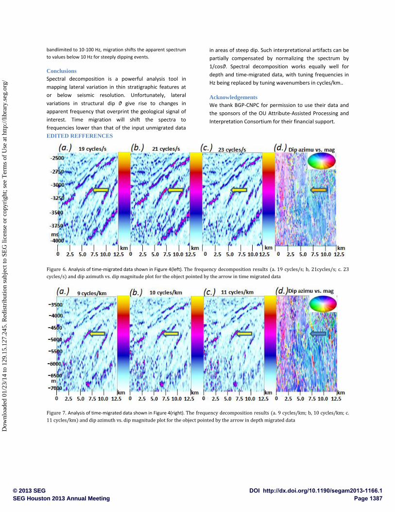
We compute the 3D dip and azimuth of the data and co-

render it with seismic amplitude in Figures 6a and 7a.

We also compute the peak spectral frequency using a

matching pursuit algorithm and display the results in

Figures 6b and 7b. Finally, we normalize the peak

freque y by dividi g by 1 θ d di pl y he re ul

in Figure 6c and 7c. As expected, the values of peak

frequency are unchanged in areas of low dip but change

significantly in areas of high dip (block arrows).

Figure 4. Seismic profile of time migrated data (left) and depth

migrated data (right).

Figure 5. Average spectra of the (top) depth-migrated and

(bottom) time-migrated data shown in Figure 4. Note the

numerical range of 2-24 cycles/km for the depth migrated data in

cycles/km is numerically lower than the 5-50 Hz range for the

time migrated data. Even if the original seismic data were


Dow

nloa

ded

01/2

3/14

to 1

29.1

5.12

7.24

5. R

edis

trib

utio

n su

bjec

t to

SEG

lice

nse

or c

opyr

ight

; see

Ter

ms

of U

se a

t http

://lib

rary

.seg

.org

/

bandlimited to 10-100 Hz, migration shifts the apparent spectrum

to values below 10 Hz for steeply dipping events.

Conclusions

Spectral decomposition is a powerful analysis tool in

mapping lateral variation in thin stratigraphic features at

or below seismic resolution. Unfortunately, lateral

variations in structural dip θ give rise to changes in

apparent frequency that overprint the geological signal of

interest. Time migration will shift the spectra to

frequencies lower than that of the input unmigrated data

in areas of steep dip. Such interpretational artifacts can be

partially compensated by normalizing the spectrum by

1/cosθ. Spectral decomposition works equally well for

depth and time-migrated data, with tuning frequencies in

Hz being replaced by tuning wavenumbers in cycles/km..

Acknowledgements

We thank BGP-CNPC for permission to use their data and

the sponsors of the OU Attribute-Assisted Processing and

Interpretation Consortium for their financial support.

EDITED REFFERENCES

Figure 6. Analysis of time-migrated data shown in Figure 4(left). The frequency decomposition results (a. 19 cycles/s; b, 21cycles/s; c. 23

cycles/s) and dip azimuth vs. dip magnitude plot for the object pointed by the arrow in time migrated data

Figure 7. Analysis of time-migrated data shown in Figure 4(right). The frequency decomposition results (a. 9 cycles/km; b, 10 cycles/km; c.

11 cycles/km) and dip azimuth vs. dip magnitude plot for the object pointed by the arrow in depth migrated data


Dow

nloa

ded

01/2

3/14

to 1

29.1

5.12

7.24

5. R

edis

trib

utio

n su

bjec

t to

SEG

lice

nse

or c

opyr

ight

; see

Ter

ms

of U

se a

t http

://lib

rary

.seg

.org

/

http://dx.doi.org/10.1190/segam2013-1166.1 EDITED REFERENCES Note: This reference list is a copy-edited version of the reference list submitted by the author. Reference lists for the 2013 SEG Technical Program Expanded Abstracts have been copy edited so that references provided with the online metadata for each paper will achieve a high degree of linking to cited sources that appear on the Web. REFERENCES

Bahorich, M., A. Motsch, K. Lauthlin , and G. Partyka, 2002, Amplitude responses image reservoir: Hart’s E&P, January, 59–61.

Laughlin , K., P. Garossino, and G. Partyka, 2002, Spectral decomp applied to 3D: AAPG Explorer, http://www.aapg.org/explorer/geophysics_corner/2002/05gpc/cfm, accessed 9 April 2005.

Hoecker, C., and G. Fehmers, 2002, Fast structural interpretation with structure-oriented filtering: The Leading Edge , 21, 238–243, http://dx.doi.org/10.1190/1.1463775.

Leppard, C., A. Eckersley, and S. Purves, 2010, Quantifying the temporal and spatial extent of depositional and structural elements in 3D seismic data using spectral decomposition and multiattribute RGB blending: 30th Annual GCSSEPM, Foundation Bob F. Perkins Research Conference, 1–10.

Liu, J. L., and K. J. Marfurt, 2007, Instantaneous spectral attributes to detect channels: Geophysics, 72, no. 2, P23–P31, http://dx.doi.org/10.1190/1.2428268.

Marfurt, K. J., R. L. Kirlin, S. H. Farmer, and M. S. Bahorich, 1998, 3D seismic attributes using a running window semblance-based algorithm: Geophysics, 63, 1150–1165. http://dx.doi.org/10.1190/1.1444415.

Partyka, G., J. Gridley, and J. A. Lopez, 1999, Interpretational applications of spectral decomposition in reservoir characterization: The Leading Edge, 18, 353–360, http://dx.doi.org/10.1190/1.1438295.

Peyton, L., R. Bottjer, and G. Partyka, 1998, Interpretation of incised valleys using new 3D seismic techniques: A case history using spectral decomposition and coherency: The Leading Edge, 17, 1294–1298, http://dx.doi.org/10.1190/1.1438127.

Widess, M. B., 1973, How thin is a thin bed?: Geophysics, 38, 1176–1180, http://dx.doi.org/10.1190/1.1440403.


Dow

nloa

ded

01/2

3/14

to 1

29.1

5.12

7.24

5. R

edis

trib

utio

n su

bjec

t to

SEG

lice

nse

or c

opyr

ight

; see

Ter

ms

of U

se a

t http

://lib

rary

.seg

.org

/

spectral decomposition of time- versus depth-migrated...

Documents