a generalized spectral decomposition technique to … · a generalized spectral decomposition...

HAL Id: hal-00366619https://hal.archives-ouvertes.fr/hal-00366619v2

Submitted on 14 Mar 2009

HAL is a multi-disciplinary open accessarchive for the deposit and dissemination of sci-entific research documents, whether they are pub-lished or not. The documents may come fromteaching and research institutions in France orabroad, or from public or private research centers.

L’archive ouverte pluridisciplinaire HAL, estdestinée au dépôt et à la diffusion de documentsscientifiques de niveau recherche, publiés ou non,émanant des établissements d’enseignement et derecherche français ou étrangers, des laboratoirespublics ou privés.

A generalized spectral decomposition technique to solvea class of linear stochastic partial differential equations

Anthony Nouy

To cite this version:Anthony Nouy. A generalized spectral decomposition technique to solve a class of linear stochasticpartial differential equations. Computer Methods in Applied Mechanics and Engineering, Elsevier,2007, 196 (45-48), pp.4521-4537. <10.1016/j.cma.2007.05.016>. <hal-00366619v2>

https://hal.archives-ouvertes.fr/hal-00366619v2

https://hal.archives-ouvertes.fr

A generalized spectral decomposition

technique to solve a class of linear stochastic

partial differential equations

Anthony Nouy a,∗

aInstitut de Recherche en Genie Civil et Mecanique (GeM), Nantes AtlanticUniversity, Ecole Centrale Nantes, UMR CNRS 6183, 2 rue de la Houssiniere,

B.P. 92208, 44322 Nantes Cedex 3

Abstract

We propose a new robust technique for solving a class of linear stochastic partial dif-ferential equations. The solution is approximated by a series of terms, each of whichbeing the product of a scalar stochastic function by a deterministic function. Noneof these functions are fixed a priori but determined by solving a problem which canbe interpreted as an ”extended” eigenvalue problem. This technique generalizes theclassical spectral decomposition, namely the Karhunen-Loeve expansion. Ad-hoc it-erative techniques to build the approximation, inspired by the power method forclassical eigenproblems, then transform the problem into the resolution of a few un-coupled deterministic problems and stochastic equations. This method drasticallyreduces the calculation costs and memory requirements of classical resolution tech-niques used in the context of Galerkin stochastic finite element methods. Finally,this technique is particularly suitable to non-linear and evolution problems since itenables the construction of a relevant reduced basis of deterministic functions whichcan be efficiently reused for subsequent resolutions.

Key words: Computational Stochastic Mechanics, Stochastic Finite Element,Spectral Decomposition, Karhunen-Loeve, Stochastic Partial DifferentialEquations

∗ Corresponding author. Tel.: +33(0)2-51-12-55-20; Fax: +33(0)2-51-12-52-52Email address: [email protected] (Anthony Nouy).

Preprint

1 Introduction

Stochastic finite element methods have been recently proposed to solve stochas-tic partial differential equations and offer a significant tool to deal with therandomness which is inherent to mechanical systems.Non-intrusive techniques, such as Monte-Carlo simulation [1,2], response sur-face method, projection [3] or regression [4] methods, have the great advan-tage that they only require the use of a simple deterministic calculation code.Stochastic problems, whatever their complexity, can be solved without anyfurther developments, as long as the associated deterministic code exists. How-ever, they require a huge number of deterministic calculations, which leads tohigh computational costs.Galerkin-type methods [5–7], which differ from one another in the choice of theapproximation space, systematically lead to a high precision solution which isexplicit in terms of the basic random variables describing the uncertainties.However, they require the resolution of a huge system of equations. Ad-hocKrylov-type iterative techniques have been proposed to make use of the spar-sity of the system [8–10]. The difficulty to build efficient preconditioners andmemory requirements induced by these techniques still limit their use to lowstochastic dimensions when dealing with large scale applications.In this paper, we propose a new alternative resolution technique to solvestochastic problems, inspired by a resolution technique for solving evolutionequations [11,12]. The idea is to approximate the solution u by:

u ≈M∑

i=1

λiUi,

where the Ui are deterministic functions and where the λi are scalar stochas-tic functions (i.e. random variables). A decomposition of this type will besaid optimal if the number of terms M is minimum for a given quality of ap-proximation. The set of deterministic (resp. stochastic) functions can be thenconsidered as an optimal deterministic (resp. stochastic) reduced basis. Here,neither the λi nor the Ui are fixed a priori. The key questions are then: howto define the ”optimal” reduced basis and how to compute it? In fact, the ob-tained decomposition depends on what we mean by ”optimal”. If we knew thesolution, the best approximation would classically be defined by minimizingthe distance to the solution in a mean square sense. In this case, it simplyleads to the classical spectral decomposition, namely the Karhunen-Loeve ex-pansion truncated at order M (see e.g. [5]). The problem is that the solution,and a fortiori its correlation, are not known. In [7], the authors propose toestimate the correlation of the solution by a Neumann expansion technique.Having the correlation, the deterministic functions are simply obtained bysolving a classical eigenproblem. The associated random variables are finallycomputed by solving the initial problem on the reduced basis of deterministic

2

functions.Here, we propose an intuitive and simple way to define the best decompo-sition, which generalizes the classical spectral decomposition. It leads to theresolution of a problem which can be interpreted as an ”extended” eigenprob-lem. Ad-hoc iterative resolution techniques, inspired by classical techniques forsolving eigenproblem, are then proposed. They transform the initial probleminto the resolution of a few uncoupled deterministic problems and stochas-tic equations. This method then drastically reduces computational costs andmemory requirements of classical resolution techniques.

The outline of the paper is as follows. In section 2, we introduce the abstractvariational formulation of a class of linear stochastic partial differential equa-tion, the discretization at the deterministic level and the stochastic modeling.In section 3, we describe the stochastic discretization and the classical Galerkinstochastic finite elements methods. Then, in section 4, we introduce the con-cept of generalized spectral decomposition. We will first focus on the caseof symmetric problems before briefly introducing the case of non-symmetricproblems. In section 5, we introduce power-type algorithms allowing to buildthe generalized spectral decomposition. Finally, in section 6, three exampleswill illustrate the efficiency of the proposed method.

2 Stochastic partial differential equation

2.1 Continuous problem

We first consider a deterministic partial differential equation which has thefollowing variational formulation: find u ∈ V such that

a(u, v) = b(v) ∀v ∈ V , (1)

where V is an appropriate space of admissible functions, a is a continuousbilinear form on V and b is a continous linear form on V .In the stochastic context, a and b forms are random. We denote by (Θ,B, P )the probability space, where Θ is the set of outcomes, B the σ-algebra ofevents and P the probability measure. We denote the bilinear and linear formsrespectively by a(·, ·; θ) and b(·; θ), which underlines their dependence on theoutcome θ. The stochastic problem now consists in finding a stochastic processu which can be viewed as a random function with value in V . Function space Vcan sometimes depend on the outcome, for example when dealing with randomgeometry [13]. Here, we consider that V does not depend on the outcome. Theappropriate function space for u can then be chosen as the tensor productspace V ⊗ S, where S is an ad-hoc function space for real-valued random

3

functions. The weak formulation of the stochastic partial differential equation(see e.g. [14,15,7]) can then be written as follows: find u ∈ V ⊗ S such that

A(u, v) = B(v) ∀v ∈ V ⊗ S, (2)

where

A(u, v) =∫

Θ

a(u(θ), v(θ); θ)dP (θ) := E(a(u, v)), (3)

B(v) =∫

Θ

b(v(θ); θ)dP (θ) := E(b(v)). (4)

E(·) denotes the mathematical expectation. In this article, we focus on thecase of a linear elliptic stochastic partial differential equation. The bilinearform A is continuous on (V ⊗ S) × (V ⊗ S) and (V ⊗ S)-coercive, and thelinear form B is continuous on V ⊗ S. We consider that S = L2(Θ, dP ) is anad-hoc choice, such that V⊗S = V⊗L2(Θ, dP ) ∼= L2(Θ, dP ;V) (see e.g. [14]).

2.2 Discretization at the deterministic level

The discretization at the deterministic level consists in searching an approxi-mation of the solution of problem (1) under the form

u =n∑

i=1

ϕiui(θ), (5)

where ui ∈ S and where ϕini=1 is a basis of a finite dimensional space Vn ⊂ V .

We will denote by u = (u1, ..., un)T ∈ Rn ⊗S the random vector of unknownsrepresenting the approximate solution. It is the solution of the following semi-discretized problem: find u ∈ Rn ⊗ S such that

E(vTAu

)= E

(vTb

)∀v ∈ Rn ⊗ S, (6)

where A : Θ → Rn×n and b : Θ → Rn are such that ∀u, v ∈ Vn, we haveP -almost surely

a(u, v; θ) = vTA(θ)u, (7)

b(v; θ) = vTb(θ). (8)

Random matrix A and random vector b inherit respectively from continuityand coercivity properties of bilinear form A and continuity property of linearform B. Then, a solution in Rn ⊗ S of problem (6) exists and is unique.

We will then denote by ‖ · ‖ the classical norm on Rn ⊗ S ∼= L2(Θ, dP ;Rn),defined by

‖u‖2 = E(uTu). (9)

4

We will denote by ((u,v)) the associated scalar product.

2.3 Stochastic modeling

We consider that the probabilistic content of the problem is represented by afinite set of random variables ξ = (ξ1, ..., ξm) : Θ −→ Rm. This is naturallythe case when A and B forms in (2) only depend on a finite set of parameterswhich are random variables. When these parameters are stochastic fields, anapproximation step can allow their expression as functions of a finite set ofrandom variables. For example, in the case of second-order random fields, suchan approximation can consist of the truncated Karhunen-Loeve expansion [5].However, in the case of non-Gaussian random fields, the probabilistic charac-terization of the obtained finite set of random variables is not trivial. Somerecent works try to answer this question by using truncated polynomial chaosexpansions of the stochastic field, the coefficients of the expansions being con-structed by the resolution of an adapted inverse problem (see e.g. [16,17]).Those techniques lead to a description of the probabilistic content by a finiteset of independent Gaussian random variables. Let us note that an approxi-mation is done on the bilinear form A. A particular care must then be takenon the truncation in order to keep coercivity properties of the approximatebilinear form [18,15] and then to ensure existence and uniqueness propertiesfor the approximate model.

After this stochastic modeling step, a random function f can then be rewrittenas a function of the basic random variables f(ξ) and the stochastic problem(2) can be equivalently formulated on the finite dimensional probability space(Θ(m),B(m), P (m)), where Θ(m) = Range(ξ) is a subset of Rm, Bm is the asso-ciated Borel σ-algebra and P (m) is the image probability measure (cf. [19,14]).In the following, for the sake of simplicity, we will still denote by (Θ,B, P ) thenew finite dimensional probability space (Θ(m),B(m), P (m)).

3 Classical stochastic finite element methods

3.1 Stochastic discretization

Classical stochastic finite element methods introduce a finite dimensional sub-space SP ⊂ S for the approximation at the stochastic level. Several choiceshave been proposed for building approximation basis; spectral approaches(polynomial chaos [20,5], generalized chaos [21]) classically use orthogonalpolynomial basis and show exponential convergence rates [21] in the case of

5

quite smooth solutions. For the case of non-smooth solutions, other approxima-tion techniques have been introduced (Wiener-Haar chaos [22], finite elements[6]).The approximation space is defined as follows:

SP = v ∈ S ; v(θ) =∑

α∈IP

Hα(θ)vα, vα ∈ R, (10)

where Hαα∈I is a basis of S and where IP is a subset of I with cardinal P .If random variables ξi are independent, S is a tensor product space S1 ⊗. . .⊗ Sm. Each dimension can be independently discretized; denoting by α =(α1, . . . , αm) ∈ Nm a multi-index, we can write Hα(θ) = h1

α1(ξ1) . . . hm

αm(ξm),

where hiαi∈ S i. In practice, we will use an orthonormal basis, i.e. E(HαHβ) =

δαβ = δα1β1 ...δαmβm .In the case of mutually dependent random variables ξi, it is possible to use gen-eralized “non-polynomial” chaos expansions [23] or more classically, to changethe basic random variables by using an adapted mapping of the ξi into inde-pendent Gaussian random variables.Below, we present a classical way of defining and computing an approximationof the solution of problem (6).

3.2 Galerkin approximation at the stochastic level

Classical Galerkin approximation of problem (6) is obtained by replacing thefunction space Vn ⊗ S by the approximation space Vn ⊗ SP . The problem isthen to find u ∈ Rn ⊗ SP such that,

E(vTAu

)= E

(vTb

)∀v ∈ Rn ⊗ SP , (11)

which leads to the following system of equations:

∑

β∈IP

E(AHαHβ)uβ = E(Hαb) ∀α ∈ IP . (12)

Denoting the solution by a block vector u, whose block α is defined by (u)α =uα, system (12) can be written

Au = b, (13)

where A and b are respectively a block matrix and a block vector. Their blocksare defined by (A)αβ = E(AHαHβ) and (b)α = E(Hαb).

6

3.3 Krylov-type iterative techniques

In practice, system (13) can not be solved by a direct resolution technique.Indeed, memory requirements and computational costs of assembling and solv-ing this huge system of size P ×n become prohibitive for large-scale engineer-ing problems. To avoid assembling and to take part of the sparsity of thissystem, we classically use a Krylov-type iterative resolution technique [8,9]such as preconditioned conjugate gradient (PCG) for symmetric problems,conjugate gradient square (CGS), etc. The resolution then only necessitatesmatrix-vector products which can be eventually parallelized [10]. The precon-ditioner M is classically taken as a block-diagonal matrix, each block beingthe inverse of the mean value of matrix A, i.e. (M)αβ = E(A)−1δαβ. The rea-son for this choice is that the preconditioner is quasi-optimal when A has lowvariance terms. As the variance of matrix A increases, the preconditioner Mbecomes less and less optimal. Iterative techniques then require a large num-ber of iterations, which can drastically increase computational costs. Memorycapacities required by these techniques can also be significant. Indeed, whendealing with such a huge system, reorthogonalization of the generated Krylovsubspace is necessary, which implies the storage of this subspace. For example,if one considers a problem with n = 105 and P = 5000, storing the solution asdouble-precision floating-point numbers requires around 4 Gigabytes. Storinga Krylov subspace of dimension only 10 then requires 40 Gigabytes!

4 Generalized spectral decomposition

4.1 Principle

Here, we try to find an approximation of the solution of problem (11) underthe form

u(θ) ≈M∑

i=1

λi(θ)Ui , (14)

where λi ∈ SP are scalar random variables and Ui ∈ Rn are deterministicvectors. A decomposition of this type will be said optimal if the number ofterms M is minimum for a given quality of approximation. The set of deter-ministic vectors (resp. stochastic functions) would then be considered as anoptimal deterministic (resp. stochastic) reduced basis. Neither the λi nor theUi are fixed a priori. The key questions are then: how to define an ”optimal”decomposition and how to compute it? The answer is of course related to whatwe mean by ”optimal”.

7

When we know the stochastic vector u, a natural way to define the ”best”approximation of the form (14) is to minimize the distance between the ap-proximation and the solution:

‖u−M∑

i=1

λiUi‖2 = minU1,...,UM∈Rn

λ1,...,λM∈SP

‖u−M∑

i=1

λiUi‖2, (15)

where ‖·‖ denotes the classical L2-norm defined in (9). It is well known that theobtained approximation is the classical Karhunen-Loeve expansion truncatedat order M (cf. [5]). Vectors Ui are the M rightmost eigenvectors of E(uuT ),which is the correlation matrix of u, and can be characterized by

p(Ui) = minV ∈Vn−i+1

maxU∈V

p(U), (16)

with p(U) =UT E(uuT )U

UTU,

where p is the classical Rayleigh quotient and Vk is the set of all k-dimensionalsubspaces of Rn. The associated λi are then obtained by λi = (UT

i Ui)−1UT

i u.

In this section, we introduce an extension of this principle in order to build adecomposition of the solution of problem (11) without knowing this solutiona priori. After an introduction of several notations and comments, we fill firstfocus on the case where operator A is symmetric before treating the generalcase.

Remark 1 In this article, we consider that the approximation space Vn⊗SP isgiven. The approximate solution u is then considered as our reference solution.For details on convergence properties of the approximation and estimation oferrors with respect to the exact solution of (2), see e.g. [14,15,24,25].

4.2 Preliminaries and notations

In the following, we will denote by W = (U1 . . .UM) ∈ Rn×M the matrixwhose columns are the deterministic vectors and by Λ = (λ1 . . . λM)T ∈ RM ⊗SP the stochastic vector whose components are the stochastic functions. Theapproximation of order M (14) will then be rewritten

u(M) =M∑

i=1

Uiλi = WΛ. (17)

When neither Λ nor W are fixed, approximation (17) is not defined uniquely.In another words, there are infinitely many choices of stochastic functionsand deterministic vectors leading to the same approximation. Indeed, for any

8

invertible matrix P ∈ RM×M , we clearly have

(WP)(P−1Λ) = WΛ. (18)

The couple composed by matrix (WP) and stochastic vector (P−1Λ) thenyield the same approximation as the couple composed by matrix (W) andstochastic vector (Λ). Therefore, without loss of generality, we can for exampleimpose orthogonality or orthonormality conditions on the λi or the Ui for thedefinition of the best approximation.

Finally, if the Ui (resp. the λi) were not linearly independent, it would beclearly possible to obtain a new decomposition of type (17) with a lower num-ber of terms by using linear combinations of the Ui (resp. the λi).

Remark 2 Random functions λiMi=1 are said “linearly independent” if they

span a M-dimensional linear subspace of SP . In the finite dimensional spaceSP , the λi can be identified with vectors λi ∈ RP whose components are thecoefficients λi,α of the λi on the basis Hαα∈IP

of SP . The property “ran-dom variables λiM

i=1 are linearly independent” is then equivalent to ”vectorsλiM

i=1 are linearly independent”, or ”the rank of matrix (λ1 . . . λM) ∈ RP×M

is M”. Of course, it does not mean that random functions are statisticallyindependent.

We will suppose that (17) is the optimal decomposition which means that theUi (resp. the λi) are linearly independent. We will denote by Gn,M = W =(U1 . . .UM) ∈ Rn×M ; rank(W) = M the set of full rank matrices and byGP,M = Λ = (λ1 . . . λM)T ∈ RM ⊗ SP ; dim(span(λiM

i=1)) = M the set oflinearly independent stochastic functions 1 .

4.3 Case of a symmetric operator A

In this section, we consider the particular case where the continuous coercivebilinear form A is also symmetric. Therefore, random matrix A, which inheritsfrom properties of A, is also symmetric. The right-hand side b is a stochasticvector.

1 span(λiMi=1) denotes the linear subspace of SP which is spanned by the set of

functions λiMi=1

9

4.3.1 Definition of the best approximation

The discretized problem (11) is equivalent to the following minimization prob-lem:

J (u) = minv∈Rn⊗SP

J (v), (19)

where J (v) = E(1

2vTAv − vTb). (20)

A natural definition for the approximation follows:

Definition 3 The best approximation of order M is defined by

J (M∑

i=1

λiUi) = minU1,...,UM∈Rn

λ1,...,λM∈SP

J (M∑

i=1

λiUi), (21)

which can be equivalently written in a matrix form:

J (WΛ) = minW∈Rn×M

Λ∈RM⊗SP

J (WΛ). (22)

4.3.2 Properties of the approximation

On one hand, the stationarity conditions of J (WΛ) with respect to Λ writes:∀Λ∗ ∈ RM ⊗ SP ,

E(Λ∗T (WTAW)Λ) = E(Λ∗TWTb). (23)

This is clearly the way we could have naturally defined the best stochasticfunctions associated with known deterministic vectors.On the other hand, the stationarity conditions with respect to W writes:∀W∗ ∈ Rn×M ,

E(ΛT (W∗TAW)Λ) = E(ΛTW∗Tb). (24)

This is still the way we could have naturally defined the best deterministicvectors associated with known stochastic functions. For example, if we imposethe λi to be the basis functions of SP , namely the Hα, equation (24) wouldsimply yields the classical solution of system (11), i.e. W = (. . .uα . . .). How-ever, the resulting approximation is the less optimal approximation since ithas the maximum number of terms M = P .

Here, we ask the best approximation for simultaneously verifying equations(23) and (24). The following proposition gives fundamental properties allow-ing to better understand the meaning of the approximation and to developcomputational resolution techniques.

10

Proposition 4 The best approximation defined by definition 3 is character-ized by:

• W maximizes on the set of full rank matrices Gn,M the functional R(W)defined by

R(W) = Trace(R(W)), (25)

with R(W) = E((WTAW)−1(WTbbTW)).

• The stochastic functions are obtained by

Λ = (WTAW)−1WTb. (26)

Moreover, the best approximation verifies

J (WΛ) = −1

2R(W). (27)

Proof. Equation (23) yields relation (26). Then, we have

J (ΛW) =1

2E(ΛTWTAWΛ)− E(ΛTWTb)

= −1

2E(ΛTWTb)

= −1

2E(bTW(WTAW)−1WTb)

= −1

2Trace(E((WTAW)−1(WTbbTW)))

= −1

2R(W).

The best deterministic vectors are then such that W ∈ Gn,M maximizesR(W). 2

Remark 5 In equation (26), we use an abuse of notation. Indeed, the quantity(WTAW)−1WTb does not necessarily belongs to RM ⊗ SP . In fact, Λ ∈RM ⊗ SP must be interpreted as the solution of problem (23). This abuse ofnotation is also made in the definition of functional R(W). In fact, it should beinterpreted as follows: R(W) = Trace(E(ΛTbTW)) where Λ is the solutionof (23).

For all invertible matrix P ∈ RM×M ,

R(WP) = P−1R(W)P, (28)

andR(WP) = R(W). (29)

11

Equation (29) is a property of homogeneity. In another words, functional Rtakes the same value for all matrices whose column vectors span a given M -dimensional linear subspace of Rn. This is related to the non-uniqueness ofthe best solution W (cf. section (4.2)). For the decomposition to be defineduniquely, we could impose orthonormality conditions on W. For example,denoting by M a symmetric definite positive matrix, the optimization problemon R could be defined on the space of M-orthogonal matrices G∗n,M = W ∈Gn,M ;WTMW = IM, where IM is the identity matrix on RM . The set G∗n,M

is called a Stiefel manifold (cf. [26]).

4.3.3 Case of deterministic operator A

In order to interpret the approximation defined in proposition 4, let us considerthe particular case where operator A is deterministic. In this case, we have

R(W) = (WTAW)−1(WT E(bbT )W). (30)

The stationarity condition of R(W) = Trace(R(W)) writes

AWR(W) = E(bbT )W, (31)

which is a classical generalized eigenproblem written in a matrix form. R(W)(resp. R(W)) is the associated matrix (resp. scalar) Rayleigh quotient. There-fore, the best W characterized in proposition 4 is such that its column vectorsspan the rightmost M -dimensional eigenspace of the generalized eigenproblem(31). A particular choice for the columns of W = (U1 . . .UM) consists of theM rightmost eigenvectors. The Ui are A-orthogonal and the associated λi arecharacterized by

λi = (UTi AUi)

−1UTi b. (32)

The couples (Ui, λi) also verify

J (M∑

i=1

λiUi) = −1

2

M∑

i=1

R(Ui). (33)

E(bbT ) is the correlation matrix of random vector b. The spectral decomposi-tion can then simply be interpreted as a truncated Karhunen-Loeve expansionof b in the metric induced by A. Here, we emphasize that the approximationis not unique. Infinitely many choices of W yield the same approximation asthe particular choice consisting of eigenvectors.

Remark 6 If we choose for the Ui the eigenvectors of the generalized eigen-problem (31), which are A-orthogonal, the associated stochastic functions areorthogonal.We have then simultaneous orthogonality properties for both thestochastic functions and the deterministic vectors. In general, this propertycan not be verified in the case of a stochastic operator A.

12

4.3.4 Interpretation and comments

Regarding the results of the previous section, functional R(W) (resp. R(W)),defined in proposition 4, will be called a ”generalized” matrix (resp. scalar)Rayleigh quotient. In particular, R has the homogeneity property (29) of aclassical Rayleigh quotient. The best approximation obtained will also becalled a generalized spectral decomposition, although there is no associatedclassical eigenproblem.One could think that since the obtained decomposition is not the Karhunen-Loeve expansion, it is not the optimal decomposition. In fact, the obtaineddecomposition is optimal with respect to the optimality criterium introducedin definition 3. Properties of random matrix A, inherited from the continuouscoercive bilinear form A, allow to define the following norm on Rn ⊗ SP :

‖v‖2A = E

(vTAv

). (34)

We can then easily show that the decomposition characterized by proposition4 verifies

‖u−WΛ‖2A = ‖u‖2

A − ‖WΛ‖2A = ‖u‖2

A −R(W). (35)

The obtained decomposition is then optimal with respect to the A-norm (34)while the direct Karhunen-Loeve expansion of the solution is optimal withrespect to the L2-norm (9).

As a last comment, let us mention that it is also possible to characterizethe best approximation by defining an optimization problem on the stochas-tic functions. We can show that the following proposition 7 is equivalent toproposition 4. For this new proposition, we use the following notations: wedenote by E(Λ ⊗ A ⊗ Λ) ∈ RM×n×n×M the four indices matrix such that(E(Λ⊗A⊗Λ))ijkl = E(λiAjkλl). We denote by E(b⊗Λ) ∈ Rn×M the matrixsuch that (E(b⊗Λ))ij = E(biλj). We then define the operation ”:” as follows:for W,W∗ ∈ Rn×M ,

W∗T : E(Λ⊗A⊗Λ) : W =∑

i,j,k,l

W ∗jiE(λiAjkλl)Wkl

= E(ΛTW∗TAWΛ).

Proposition 7 The best approximation defined by definition 3 is character-ized by:

• Λ maximizes on GP,M the functional R(Λ) defined by

R(Λ) = E(Λ⊗ b) : E(Λ⊗A⊗Λ)−1 : E(b⊗Λ). (36)

• The deterministic vectors are obtained by

WT = E(Λ⊗A⊗Λ)−1 : E(b⊗Λ). (37)

13


J (WΛ) = −1

2R(Λ). (38)

4.3.5 Another definition of the approximation

The best approximation can also be naturally defined by the following opti-mization problems, which define the couples (λi,Ui) one after the other:

Definition 8 The best approximation of order M can be defined recursively:for i = 1, ..., M

J (λiUi) = minU∈Rn,λ∈SP

J (λU +i−1∑

j=1

λjUj) (39)

Following the proof of proposition 4, we obtain the following characterizationof the new obtained approximation.

Proposition 9 The approximation defined in definition 8 can be charaterizedby 2

• Ui maximizes the generalized Rayleigh quotient

Ri(U) = E(UTbi(UTAU)−1bT

i U)

with bi = b−i−1∑

j=1

AλjUj

• λi = (UTi AUi)

−1UTi bi.


J (M∑

i=1

λiUi) = −1

2

M∑

i=1

Ri(Ui). (40)

In the case of a deterministic operator, we can easily show that definitions 8and 3 yield the same approximation. However, these definitions do not matchin general in the case of a stochastic operator. Definition 3 then clearly yieldsa better approximation as definition 8. The latter definition can however beinteresting from a computational point of view, as we will see in section 5.

2 We use the same abuse of notation as in proposition 4, explained in Remark 5

14

4.4 Case of a non-symmetric operator

For the case of non-symmetric operator, there is no direct minimization prob-lem associated with the variational formulation (6). A possible and naturalway to define an approximation WΛ is to write the two orthogonality criteria(23) and (24) which can be obtained by introducing in (6) test functions of theform v = WΛ∗+W∗Λ. In the case of a non-symmetric deterministic operatorA, we can easily show that it leads to a classical non-symmetric generalizedeigenproblem. Therefore, the approximation still has a full meaning but nocharacterization as the one in proposition 4 can be derived.

Another idea consists in reformulating the problem as a minimization problemin a least-square sense. Let us denote by M ∈ Rn×n a symmetric positivedefinite matrix which defines the following scalar product on Rn ⊗ SP :

((U,V))M = E(UTMV). (41)

We will denote by ‖ · ‖M the associated norm. For example, if the expectedvalue of the symmetric part of A is positive definite, we can take M = (1

2E(A+

AT ))−1. We can then formulate the problem as a minimization problem of thenorm of the residual:

E(u) = minv∈Rn⊗SP

E(v) (42)

where E(v) = ‖b−Av‖2M.

The previous theoretical results associated with symmetric operators can thenbe still applied by replacing operator A by ATMA and right hand side b byATMb. Of course, the approximate solution of this problem is not in generalthe same as for problem (11) when A is random.

Although this symmetrization is well adapted to the discretized formulation(finite dimensional framework), it is not easy to transpose into the continuousframework. Indeed, the introduction of adjoint operator is non trivial, essen-tially due to the treatment of boundary conditions. Moreover, ad-hoc functionspaces need for more regularity after symmetrization and the building of ap-proximation spaces is then more difficult.

However, we will see that this symmetrization does not seem necessary since al-gorithms which are given in the following section also gives satisfactory resultswhen directly applied to non-symmetric problems. Without the symmetry, wedo not have an optimality criterium as in proposition 4. It is then more difficultto judge the quality of the approximation. Of course, it is possible to evaluatethe norm of the residual of equation (11) but this increases computationalcosts.

15

5 Power-type algorithms for the construction of the spectral de-composition

5.1 Description of the algorithm

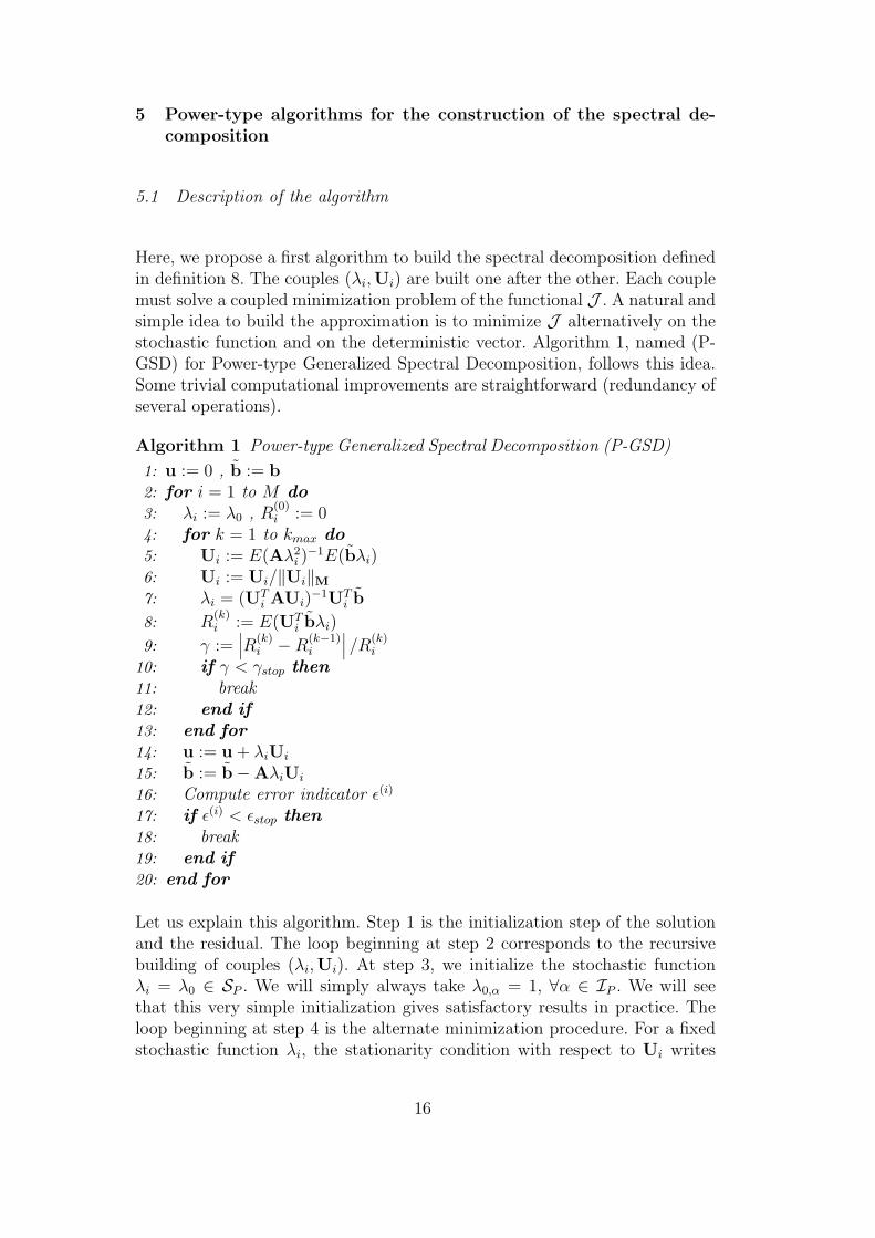
Here, we propose a first algorithm to build the spectral decomposition definedin definition 8. The couples (λi,Ui) are built one after the other. Each couplemust solve a coupled minimization problem of the functional J . A natural andsimple idea to build the approximation is to minimize J alternatively on thestochastic function and on the deterministic vector. Algorithm 1, named (P-GSD) for Power-type Generalized Spectral Decomposition, follows this idea.Some trivial computational improvements are straightforward (redundancy ofseveral operations).

Algorithm 1 Power-type Generalized Spectral Decomposition (P-GSD)

1: u := 0 , b := b2: for i = 1 to M do3: λi := λ0 , R

(0)i := 0

4: for k = 1 to kmax do5: Ui := E(Aλ2

i )−1E(bλi)

6: Ui := Ui/‖Ui‖M7: λi = (UT

i AUi)−1UT

i b

8: R(k)i := E(UT

i bλi)

9: γ :=∣∣∣R(k)

i −R(k−1)i

∣∣∣ /R(k)i

10: if γ < γstop then11: break12: end if13: end for14: u := u + λiUi

15: b := b−AλiUi

16: Compute error indicator ε(i)

17: if ε(i) < εstop then18: break19: end if20: end for

Let us explain this algorithm. Step 1 is the initialization step of the solutionand the residual. The loop beginning at step 2 corresponds to the recursivebuilding of couples (λi,Ui). At step 3, we initialize the stochastic functionλi = λ0 ∈ SP . We will simply always take λ0,α = 1, ∀α ∈ IP . We will seethat this very simple initialization gives satisfactory results in practice. Theloop beginning at step 4 is the alternate minimization procedure. For a fixedstochastic function λi, the stationarity condition with respect to Ui writes

16

E(Aλ2i )Ui = E(bλi). It has to be noticed that it is a simple deterministic

problem whose resolution is relatively cheap. This system is solved at step5 and Ui is normalized at step 6. In the symmetric case, we simply takeM = E(A) for the definition of the norm. Then, for a fixed Ui, the stationaritycondition with respect to λi writes

E(λ∗UTi AUiλi) = E(λ∗UT

i b) ∀λ∗ ∈ SP . (43)

This system is solved at step 7. From step 8 to step 12, we introduce a stop-ping criterium based on the convergence of the quantity R

(k)i . This quantity

corresponds to the generalized Rayleigh quotient in the case where operator Ais symmetric (see definition 8). At steps 14 and 15, we reactualize the solutionand the residual. From 16 to 19, we introduce a stopping criterium. The errorindicator can be the residual error

ε(i)res =

‖b−A∑i

j=1 λjUj‖‖b‖ . (44)

Regarding the results of proposition 9, we can also use the following errorindicator, based on the generalized Rayleigh quotient evaluation:

ε(i)ray =

Ri(Ui)∑ij=1 Rj(Uj)

. (45)

This last indicator has the advantage to be cheaper to compute. Indicators(44) and (45) will be compared in section 6.

Remark 10 Computing the matrix and right-hand side of the deterministicproblem (step 5) requires the computation of quantities such as E(Aλiλj) orE(bλi). This kind of computations are classical within the context of stochasticfinite element methods. Let us consider that the random vector b is decom-posed as follows: b =

∑Mbk=1 bk(θ)bk, with bk(θ) =

∑α∈IP

bk,αHα(θ) ∈ SP .Then, due to orthonormality property of the basis functions Hα, E(bλi) =∑Mb

k=1 bk∑

α∈IPbk,αλi,α. Let us now consider that the random matrix writes

as follows: A =∑MA

k=1 ak(θ)Ak, where the ak are random variables. ThenE(Aλiλj) =

∑MAk=1 AkE(akλiλj). In practice, one pre-computes and stores the

matrices ∆(k) whose components are (∆(k))αβ = E(akHαHβ) and such thatE(akλiλj) =

∑α,β∈IP

(∆(k))αβλi,αλj,β. If the ak are decomposed on the stochas-

tic basis, i.e. ak(θ) =∑

γ ak,γHγ(θ), then (∆(k))αβ =∑

γ ak,γE(HγHαHβ),where E(HγHαHβ) only depends on the chosen basis functions Hα.

5.2 Interpretation and comments

In the case of deterministic operator, iteration k of the alternate minimiza-tion stage consists in reactualizing the deterministic vector in the following

17

way: Ui ← A−1E(bbT )Ui/η, where η is a normalizing scalar. The proposedalgorithm is then equivalent to a classical power method to solve the asso-ciated generalized eigenproblem AUi = ηE(bbT )Ui. It classically convergestoward the rightmost eigenvector. We will see in examples that this algorithmis also efficient in the case of stochastic operator. In practice, the alternateminimization procedure (steps 4 to 13) converges very fast. We will then clas-sically limit the number of iterations kmax to 3 or 4. In the case of deterministicnon-symmetric operator, we know that the proposed power algorithm is notalways convergent. If the maximum amplitude eigenvalue is complex, the gen-eralized eigenproblem admits 2 complex conjugate eigenvalues. Vector Ui doesnot converge in this case. However, it tends to stay in the subspace generatedby the real and complex parts of the associated complex eigenvectors and theobtained couple (λi,Ui) still happens to be pertinent. We will see in examplesthat this algorithm also gives satisfactory results in the general case of randomeventually non-symmetric operators.

5.3 Power-type algorithm with updating

Let us suppose we have built an approximation∑M

i=1 λiUi = WΛ. We haveseen that optimality depends on the way we define the ”best” decomposi-tion. Indeed, definitions 3 and 8 match only in the case where operator A isdeterministic. Once we have obtained such a decomposition, it can then beinteresting to update the decomposition. A natural way to do this is to fixthe deterministic vectors Ui and to compute new stochastic functions λi ∈ SP

by using a Galerkin orthogonality criterium (23). The updating can then beformulated: find Λ ∈ RM ⊗ SP such that ∀Λ∗ ∈ RM ⊗ SP ,

E(Λ∗T (WTAW)Λ) = E(Λ∗TWTb). (46)

To obtain the solution Λ(θ) =∑

α∈IPΛαHα(θ), we then have to solve a system

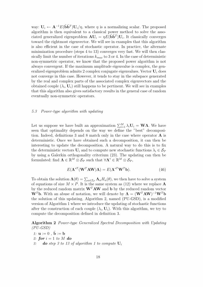
of equations of size M × P . It is the same system as (12) where we replace Aby the reduced random matrix WTAW and b by the reduced random vectorWTb. With an abuse of notation, we will denote by Λ = (WTAW)−1WTbthe solution of this updating. Algorithm 2, named (PU-GSD), is a modifiedversion of Algorithm 1 where we introduce the updating of stochastic functionsafter the construction of each couple (λi,Ui). With this algorithm, we try tocompute the decomposition defined in definition 3.

Algorithm 2 Power-type Generalized Spectral Decomposition with Updating(PU-GSD)

1: u := 0 , b := b2: for i = 1 to M do3: do step 3 to 13 of algorithm 1 to compute Ui

18

4: W := (U1 ... Ui)5: Λ := (WTAW)−1WTb6: u := WΛ7: b = b−AWΛ8: Compute error indicator ε(i)

9: if ε(i) < εstop then10: break11: end if12: end for

Regarding the results of proposition 4, we can here use an error criteriumbased on the evaluation of the generalized Rayleigh quotient

ε(i)ray =

∣∣∣∣∣R(W(i))−R(W(i−1))

R(W(i))

∣∣∣∣∣ , (47)

where W(j) = (U1 . . .Uj). We recall that at step 8, the generalized Rayleighquotient can be simply computed as follows R(W) = Trace(E(ΛbTW)).

6 Examples

The following three examples illustrate the efficiency of the proposed methodon model problems. In example 1, the method is applied to a classical sta-tionary heat diffusion problem with random source terms and a conductivityparameter which is modeled by a random field. In example 2, we considerthe same problem but with a conductivity parameter modeled by a randomvariable. It is a degenerate case of the previous example (simple form of therandom matrix), for which the solution is exactly represented with a decom-position of order 2. It illustrates that the proposed algorithms allow to au-tomatically construct this exact decomposition. Finally, example 3 illustratesthat the proposed algorithms are still efficient in the non-symmetric case.

6.1 Example 1

6.1.1 Description of the problem

[Fig. 1 about here.]

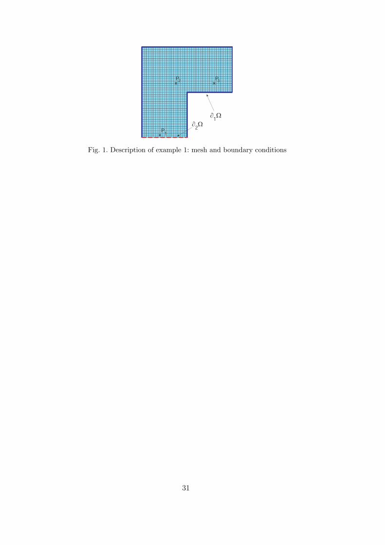
As a first model problem, we consider a classical stationary heat diffusionproblem defined on a L-shaped spatial domain Ω (see figure 1). We denote byu(x, θ) the temperature field. The normal flux g is imposed on a part ∂2Ω of theboundary and the temperature is imposed to be zero on the complementary

19

part ∂1Ω. A volumic heat source f is also imposed on Ω. The space of admis-sible functions used in formulation (1) is V = v(x) ∈ H1(Ω) ; v = 0 on ∂1Ω.In variational formulation (2), a and b forms are respectively

a(u, v; θ) =∫

Ωκ∇u · ∇v dx,

b(v; θ) =∫

Ωfv dx +

∫

∂2Ωgv ds,

where κ(x, θ) is the conductivity parameter. At the space level, we use aclassical finite element approximation. The mesh is composed by 1200 four-nodes elements and 1281 nodes. Random matrix A and random vector b,respectively defined in (7) and (8), have the following components:

(A)ij =∫

Ωκ∇ϕi · ∇ϕj dx

(b)j =∫

Ωfϕj dx +

∫

∂2Ωgϕj ds,

where the ϕi are the basis functions of the approximation space Vn ⊂ V .

6.1.2 Stochastic modeling

The conductivity parameter is modeled by a random field. The following defi-nition is taken from [17], where it was used to illustrate a method for identifica-tion of non-Gaussian random fields. Here, this definition allows us to impose agiven marginal distribution which simply ensures the ellipticity of the bilinearform. We take

κ(x, θ) = F−1Γδ Φ(γ(x, θ))),

where γ is a normalized Gaussian second-order random field such that E(γ(x, ·)) =0 and E(γ(x, ·)2) = 1. Function y → Φ(y) is the cumulative distribution func-tion of a normalized Gaussian random variable and function y → FΓδ

(y) isthe cumulative distribution function of a Gamma random variable:

FΓδ(y) =

∫ y

0

δ

Γ(δ)(δt)δ−1e−δt dt,

with Γ(δ) =∫ ∞

0tδ−1e−t dt.

With this definition, κ has a Gamma marginal distribution with unitary meanand standard deviation σ = 1/

√δ. We take δ = 16 so that σ = 0.25. The

Gaussian random field γ(x, θ) is here defined by

γ(x, θ) =3∑

k=1

√ηkξk(θ)Vk(x), (48)

with Vk(x) =Vk(x)√∑3

j=1 ηjVj(x)2,

20

where the ξk ∈ N (0, 1) 3 are independent normalized Gaussian random vari-ables and where (ηk, Vk(x)) are the eigenpairs of the following homogeneousFredholm equation of the second kind:

∫

Ωexp(−‖x− y‖2

L2)Vk(y)dy = ηkVk(x). (49)

Then, the random field γ corresponds to a rescaled truncated Karhunen-Loeveexpansion of a Gaussian random field with exponential square correlation func-tion. We take L = 0.5. In practice, problem (49) can be approximated by usingfinite elements. Here, we use the same approximation as for the solution u. Wethen have to solve a classical algebraic eigenvalue problem (cf. [5]). We use aclassical technique to find its 3 rightmost eigenpairs.

Volumic heat source f and normal flux g are taken independent of the variablex: f(x, θ) = ξ4(θ) ∈ N (0.5, 0.2) and g(x, θ) = ξ5(θ) ∈ N (0, 0.2), where ξ4 andξ5 are independent Gaussian random variables, also independent of ξi3

i=1.The source of randomness is then represented by m = 5 independent Gaussianrandom variables. We use a polynomial chaos approximation of degree p = 6at the stochastic level. The dimension of approximation space SP is thenP = (m+p)!

m!p!= 462.

The random field κ is projected on SP : κ(x, θ) =∑

α∈IPκα(x)Hα(θ) where

space functions κα = E(κHα) are computed using Gauss-Hermite quadraturefor the integration at the stochastic level. Matrix A can then be written A =∑

α∈IPAαHα with (Aα)ij =

∫Ω κα∇ϕi · ∇ϕj dx.

6.1.3 Reference solution and error criteria

We denote by u(M) the approximation of order M (14) obtained by the gener-alized spectral decomposition algorithms, namely the power-type algorithms(P-GSD) or (PU-GSD). We denote by u the reference solution, which is thesolution of (11). To compute u, system (12) is solved with a preconditionedconjugate gradient (PCG) (see section 3.2), with a stopping tolerance of 10−8.We introduce the following error indicators to evaluate the quality of the ap-proximation:

ε(M)sol =

‖u− u(M)‖‖u‖ , ε

(M)sol,A =

‖u− u(M)‖A‖u‖A . (50)

where ‖·‖ is the classical L2-norm (9) and ‖·‖A is the A-norm defined in (34).The generalized spectral decomposition obtained by power-type algorithmswill be also compared with the direct Karhunen-Loeve spectral decompositionof the reference solution u, denoted by (Direct-SD).

3 N (µ, σ) denotes the set of Gaussian random variables with mean µ and standarddeviation σ

21

Remark 11 Of course, approximations are first introduced by the spatial andstochastic discretizations. The error introduced by the stochastic discretizationcan be defined by the difference between our reference solution u and the solu-tion of the semi-discretized problem (6). For this example, we estimated thiserror by computing the discretized solution associated with a polynomial chaosof degree p = 8. The estimation of the relative error in L2-norm is 1.04 10−2.In this article, we don’t focus on those errors and consider the reference so-lution as the solution of the fully discretized problem (11). However, this re-mark indicates that a very small tolerance for the resolution of the discretizedproblem (11) is generally useless for engineering applications, for which thediscretization error is often greater than 1%.

6.1.4 Convergence of power-type algorithms

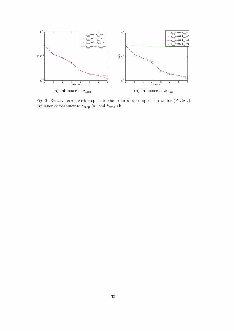
(P-GSD) and (PU-GSD) have two parameters which are associated with theiterative search of each couple of functions (steps 3 to 13 of Algorithm 1): γstop,which defines the stopping criterium, and kmax, which defines the maximumnumber of iterations. Figures 2(a) and 2(b) show the error ε

(M)sol with respect

to the order M of the decomposition for different values of these parameters.On one hand, figure 2(a) shows that a relatively coarse convergence criterium(γstop ≈ 0.1) do not affect the quality of the decomposition. On another hand,figure 2(b) shows that for a fixed stopping criterium γstop = 0.05, a few it-erations are sufficient, which is in fact related to the fast convergence of thisiterative procedure. For the following tests, we will choose γstop = 0.05 andkmax = 3.


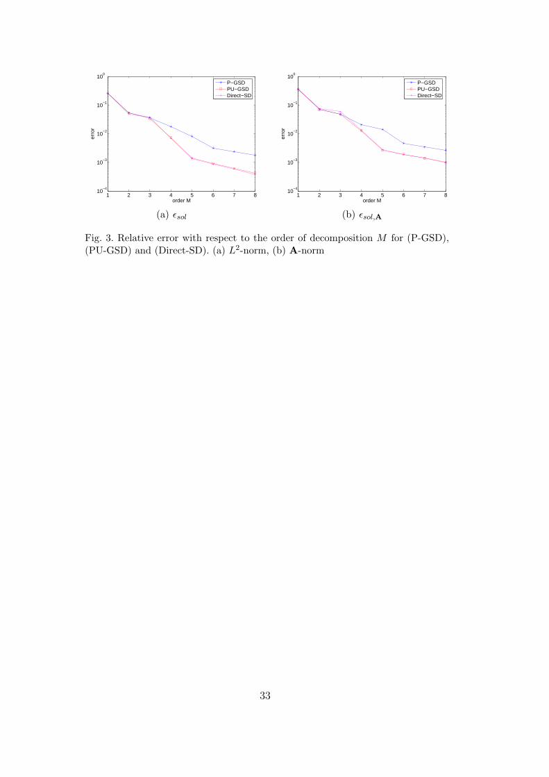
Figures 3(a) and 3(b) compare the convergence of (P-GSD), (PU-GSD) and(Direct-SD) with respect to the order of expansion M . We can observe that(PU-GSD) has almost the same convergence rate as (Direct-SD). This fig-ure also shows the importance of the updating of stochastic functions. In-deed, without knowing the solution a priori, algorithm (PU-GSD) leads toa spectral decomposition of the solution which has quite the same qualityas a direct Karhunen-Loeve decomposition of the reference solution. We alsoverify, as mentioned in section 4.3.4, that (Direct-SD), when compared with(PU-GSD), gives a better approximation with respect to the L2-norm but acoarser approximation with respect to the A-norm. We can also notice thanwith a decomposition of order M = 4, the error is less than 1%.


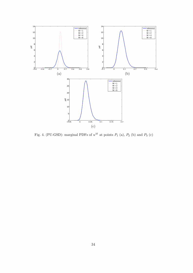
Figures 4(a),4(b) and 4(c) show the marginal probability density functions(PDFs) of the approximation obtained by (PU-GSD) for different orders ofexpansion M . The three sub-figures correspond respectively to points P1, P2

22

and P3 (see figure 1). We can observe that with an approximation of orderonly M = 4, the approximate PDFs fit very well the reference solution.


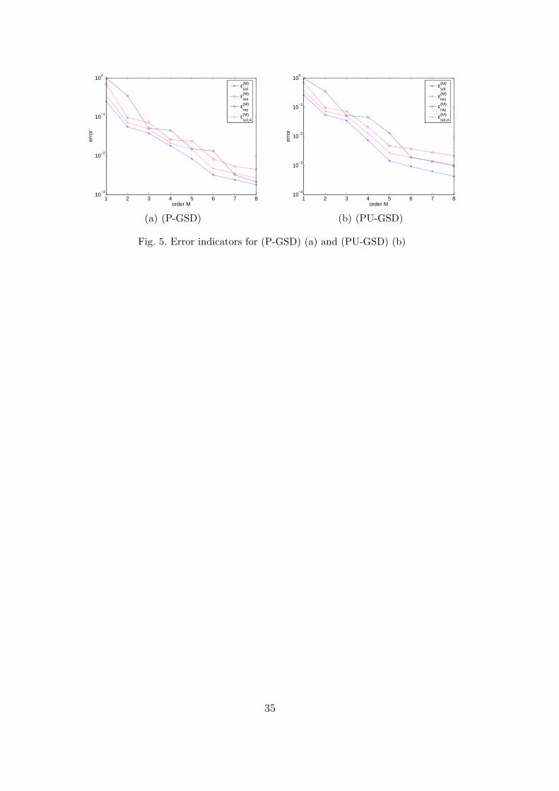
Figures 5(a) and 5(b) compare error indicators εray and εres which can beused to evaluate the convergence of algorithms (P-GSD) and (PU-GSD). εres

is the norm of the residual, defined in (44), and εray is the indicator basedon the Rayleigh quotient, defined in (45) for (P-GSD) and in (47) for (PU-GSD). These error indicators are compared to error indicators εsol and εsol,A,defined in (50). We can see that all these indicators are equivalent. The greatadvantage of estimator εray is that it leads to very low computational costs.


6.1.5 Analysis of the generalized spectral decomposition

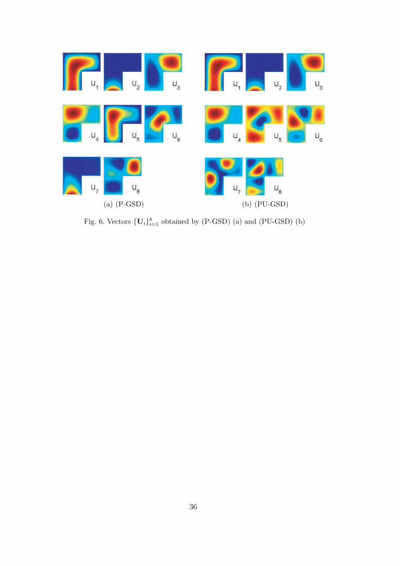
Figures 6(a) and 6(b) show the first 8 deterministic vectors obtained respec-tively by (P-GSD) and (PU-GSD). We observe that these algorithms yield tothe construction of quite relevent deterministic vectors. Vectors 1 and 2 takerespectively into account the volumic load f and the surface load g. Subse-quent vectors seem to take into account the fluctuations of the conductivityparameter. The superiority of (PU-GSD) appears clearly on this figure. In-deed, vectors 5 and 7 obtained by (P-GSD) are very similar to vectors 1 and2. In fact, they can be interpreted as correction terms for the first two modes.Algorithm (PU-GSD) seems to capture these modes with the first two vectorsand does not require any further correction.


Figure 7 shows the 8 first vectors computed by a direct Karhunen-Loeve de-composition of the reference solution (Direct-SD). If we compare this figurewith figure 6 (b), we can see that (PU-GSD) and (Direct-SD) lead to very simi-lar decompositions. In fact, we can say that the proposed algorithm (PU-GSD)allows to obtain a spectral decomposition of the solution, which is very similarto the Karhunen-Loeve expansion, without knowing the solution a priori.


6.1.6 Calculation time and memory requirements

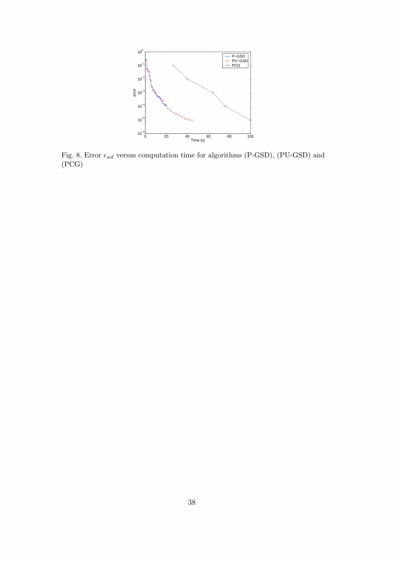
We now look at the computation time of the proposed algorithms. Algorithm(PCG) took 156 s to compute the reference solution. Figure 8 shows the er-ror with respect to the calculation time for (P-GSD), (PU-GSD) and (PCG)

23

algorithms. The convergence curves for (P-GSD) and (PU-GSD) correspondto a generalized spectral decomposition up to order M = 20. We observethat power-type algorithms lead to the same computational cost. (PU-GSD)converges faster with respect to the order M but the cost of one iteration isgreater than for (P-GSD), due to the updating of stochastic functions. On thisexample, we can then conclude that (PU-GSD) is more efficient since it leadsto a decomposition with a lower order M for the same accuracy and calcu-lation time. We see that power-type algorithms are significatively superior tothe classical (PCG) algorithm. To compute a decomposition of order M = 4,which leads to a relatively good accuracy, it only takes 3.5 s with (PU-GSD).The same accuracy is reached in 40 s with (PCG). The calculation time isthen divided by 11 on this simple example.


To store the spectral decomposition of order M , we need to store M × (P +n) floating-point numbers. For (PCG) we need to store n × P floating-pointnumbers. For an approximation of order M = 4, memory requirements aredivided by around 85. In fact, the gain is much greater since (PCG) algorithmgenerally requires reorthogonalization of the search directions. In fact, thestorage of a Krylov subspace of dimension η requires to store η × n × Pfloating-point numbers.

6.2 Example 2

We consider the same problem as in example 1. The linear form b(v; θ) is un-changed. The sources f and g are still defined by f(x, θ) = ξ4(θ) ∈ N (0.5, 0.2)and g(x, θ) = ξ5(θ) ∈ N (0, 0.2). But now, we suppose that the conductivity isa simple uniform random variable κ(x, θ) = ξ1 ∈ U(0.7, 1.3) 4 . Random vari-ables ξ1, ξ4, ξ5 are considered independent. We use a generalized polynomialchaos approximation of degree p = 8 at the stochastic level [21]. We then useLegendre polynomials in the first stochastic dimension and Hermite polyno-mials in the two other stochastic dimensions. The dimension of approximationspace SP is then P = (m+p)!

m!p!= 165, where m = 3.


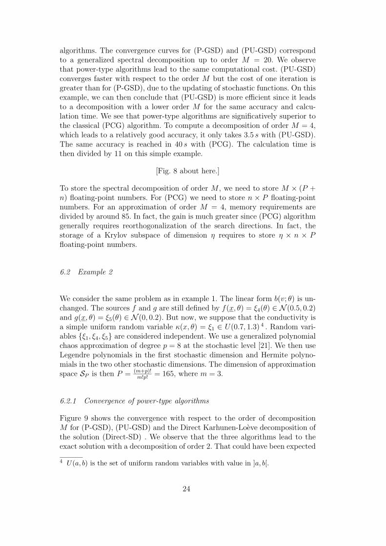
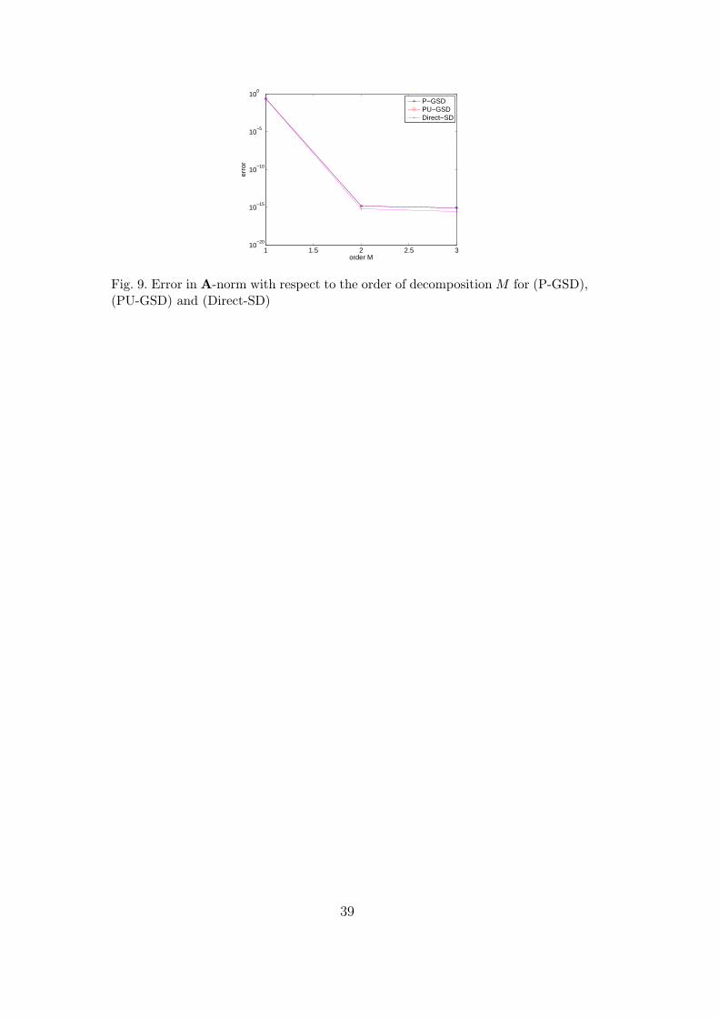
Figure 9 shows the convergence with respect to the order of decompositionM for (P-GSD), (PU-GSD) and the Direct Karhunen-Loeve decomposition ofthe solution (Direct-SD) . We observe that the three algorithms lead to theexact solution with a decomposition of order 2. That could have been expected

4 U(a, b) is the set of uniform random variables with value in ]a, b[.

24

since the random matrix can be written A = ξ1A1 where A1 is a deterministicmatrix and the right hand side can be written b = ξ4b4 + ξ5b5, where b4 andb5 are deterministic vectors.


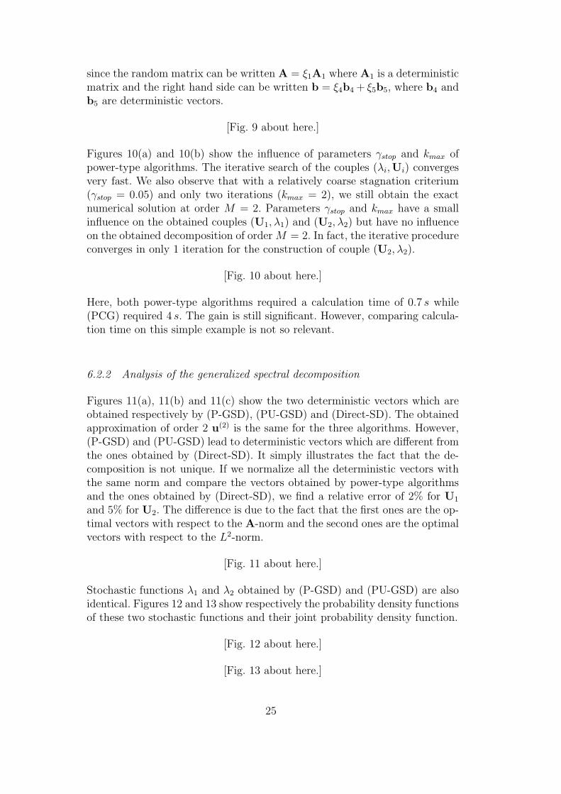
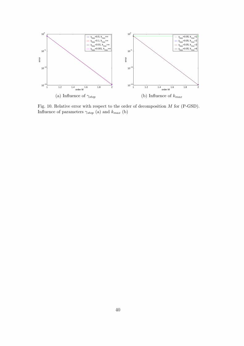
Figures 10(a) and 10(b) show the influence of parameters γstop and kmax ofpower-type algorithms. The iterative search of the couples (λi,Ui) convergesvery fast. We also observe that with a relatively coarse stagnation criterium(γstop = 0.05) and only two iterations (kmax = 2), we still obtain the exactnumerical solution at order M = 2. Parameters γstop and kmax have a smallinfluence on the obtained couples (U1, λ1) and (U2, λ2) but have no influenceon the obtained decomposition of order M = 2. In fact, the iterative procedureconverges in only 1 iteration for the construction of couple (U2, λ2).


Here, both power-type algorithms required a calculation time of 0.7 s while(PCG) required 4 s. The gain is still significant. However, comparing calcula-tion time on this simple example is not so relevant.


Figures 11(a), 11(b) and 11(c) show the two deterministic vectors which areobtained respectively by (P-GSD), (PU-GSD) and (Direct-SD). The obtainedapproximation of order 2 u(2) is the same for the three algorithms. However,(P-GSD) and (PU-GSD) lead to deterministic vectors which are different fromthe ones obtained by (Direct-SD). It simply illustrates the fact that the de-composition is not unique. If we normalize all the deterministic vectors withthe same norm and compare the vectors obtained by power-type algorithmsand the ones obtained by (Direct-SD), we find a relative error of 2% for U1

and 5% for U2. The difference is due to the fact that the first ones are the op-timal vectors with respect to the A-norm and the second ones are the optimalvectors with respect to the L2-norm.


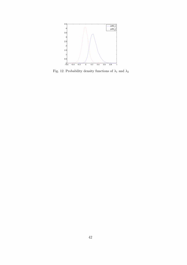
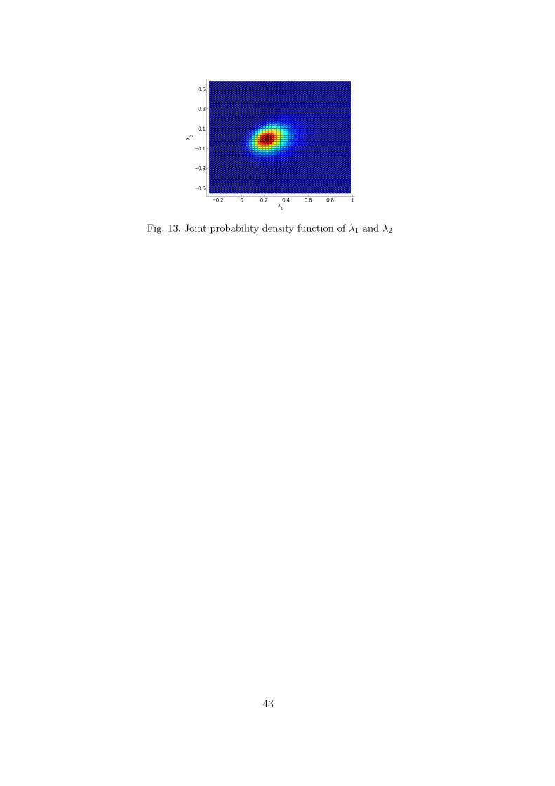
Stochastic functions λ1 and λ2 obtained by (P-GSD) and (PU-GSD) are alsoidentical. Figures 12 and 13 show respectively the probability density functionsof these two stochastic functions and their joint probability density function.



25

6.3 Example 3

In this last example, we briefly illustrate the fact that power-type algorithmsalso lead to satisfactory performances in the non-symmetric case. We hereconsider the same domain and boundary conditions as in example 1. Thelinear form b(v; θ) is unchanged but we take the following non symmetricbilinear form:

a(u, v; θ) =∫

Ωκ∇u · ∇v dx−

∫

Ωχ u · ∇v dx,

where χ = (χ1, χ2)T . We consider that material parameters are uniform ran-

dom variables: κ(x, θ) = ξ1(θ) ∈ U(0.7, 1.3), χ1(x, θ) = ξ2(θ) ∈ U(5.5, 6.5),χ2(x, θ) = ξ3(θ) ∈ U(5.5, 6.5). The five random variables ξi5

i=1 are indepen-dent. We use a generalized polynomial chaos approximation of degree p = 5.We then use Legendre polynomials in the first three stochastic dimensions andHermite polynomials in the last two stochastic dimensions. We can notice thatA still defines a norm ‖ ‖A since its symmetric part is almost surely positivedefinite. The reference solution, which solves system (12), is computed with apreconditionned conjugate gradient square algorithm (PCGS) with a stoppingtolerance of 10−8.


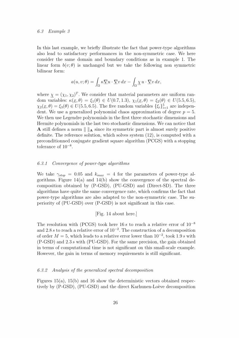
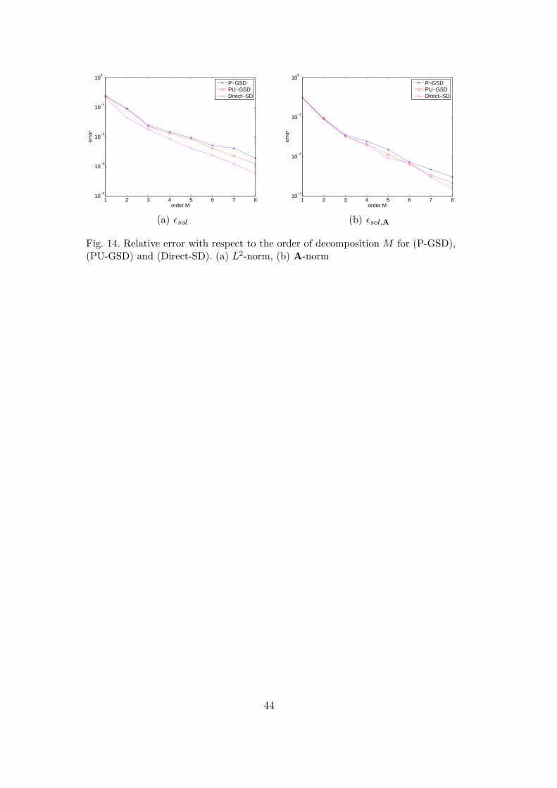
We take γstop = 0.05 and kmax = 4 for the parameters of power-type al-gorithms. Figure 14(a) and 14(b) show the convergence of the spectral de-composition obtained by (P-GSD), (PU-GSD) and (Direct-SD). The threealgorithms have quite the same convergence rate, which confirms the fact thatpower-type algorithms are also adapted to the non-symmetric case. The su-periority of (PU-GSD) over (P-GSD) is not significant in this case.


The resolution with (PCGS) took here 16 s to reach a relative error of 10−8

and 2.8 s to reach a relative error of 10−2. The construction of a decompositionof order M = 5, which leads to a relative error lower than 10−2, took 1.9 s with(P-GSD) and 2.3 s with (PU-GSD). For the same precision, the gain obtainedin terms of computational time is not significant on this small-scale example.However, the gain in terms of memory requirements is still significant.


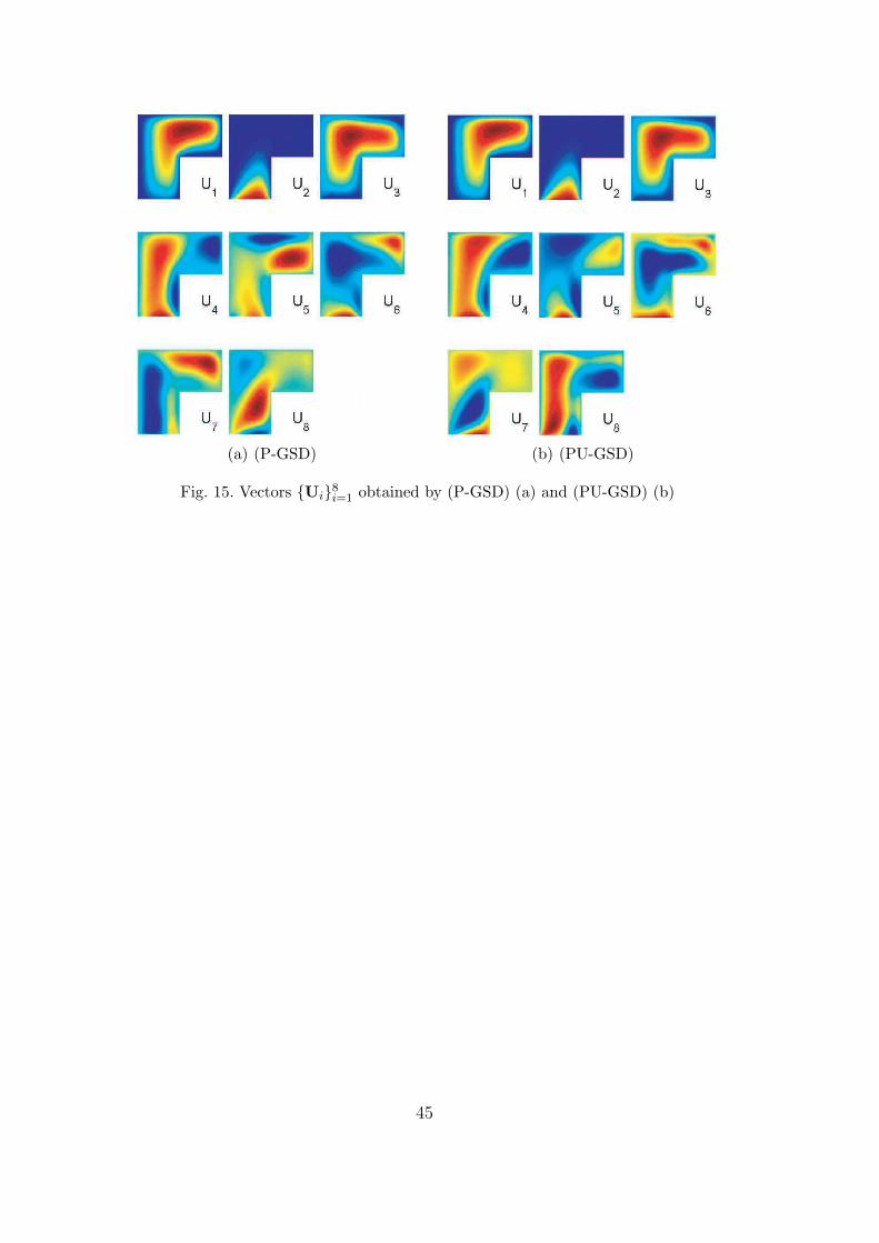
Figures 15(a), 15(b) and 16 show the deterministic vectors obtained respec-tively by (P-GSD), (PU-GSD) and the direct Karhunen-Loeve decomposition

26

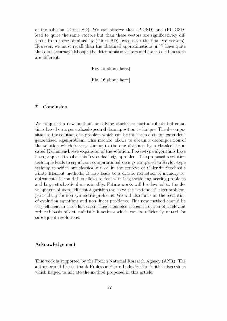
of the solution (Direct-SD). We can observe that (P-GSD) and (PU-GSD)lead to quite the same vectors but than these vectors are significatively dif-ferent from those obtained by (Direct-SD) (except for the first two vectors).However, we must recall than the obtained approximations u(M) have quitethe same accuracy although the deterministic vectors and stochastic functionsare different.



7 Conclusion

We proposed a new method for solving stochastic partial differential equa-tions based on a generalized spectral decomposition technique. The decompo-sition is the solution of a problem which can be interpreted as an ”extended”generalized eigenproblem. This method allows to obtain a decomposition ofthe solution which is very similar to the one obtained by a classical trun-cated Karhunen-Loeve expansion of the solution. Power-type algorithms havebeen proposed to solve this ”extended” eigenproblem. The proposed resolutiontechnique leads to significant computational savings compared to Krylov-typetechniques which are classically used in the context of Galerkin StochasticFinite Element methods. It also leads to a drastic reduction of memory re-quirements. It could then allows to deal with large-scale engineering problemsand large stochastic dimensionality. Future works will be devoted to the de-velopment of more efficient algorithms to solve the ”extended” eigenproblem,particularly for non-symmetric problems. We will also focus on the resolutionof evolution equations and non-linear problems. This new method should bevery efficient in these last cases since it enables the construction of a relevantreduced basis of deterministic functions which can be efficiently reused forsubsequent resolutions.

Acknowledgement

This work is supported by the French National Research Agency (ANR). Theauthor would like to thank Professor Pierre Ladeveze for fruitful discussionswhich helped to initiate the method proposed in this article.

27

References

[1] R. E. Caflisch, Monte carlo and quasi-monte carlo methods, Acta. Numer. 7(1998) 1–49.

[2] M. Papadrakakis, V. Papadopoulos, Robust and efficient methods for stochasticfinite element analysis using monte carlo simulation, Computer Methods inApplied Mechanics and Engineering 134 (1996) 325–340.

[3] B. Puig, F. Poirion, C. Soize, Non-gaussian simulation using hermite polynomialexpansion: convergences, Probabilistic Engineering Mechanics 17 (2002) 253–264.

[4] M. Berveiller, B. Sudret, M. Lemaire, Stochastic finite element: a non intrusiveapproach by regression, European Journal of Computational Mechanics 15(2006) 81–92.

[5] R. Ghanem, P. Spanos, Stochastic finite elements: a spectral approach, Springer,Berlin, 1991.

[6] M. Deb, I. Babuska, J. T. Oden, Solution of stochastic partial differentialequations using galerkin finite element techniques, Computer Methods inApplied Mechanics and Engineering 190 (2001) 6359–6372.

[7] H. G. Matthies, A. Keese, Galerkin methods for linear and nonlinearelliptic stochastic partial differential equations, Computer Methods in AppliedMechanics and Engineering 194 (12-16) (2005) 1295–1331.

[8] R. G. Ghanem, R. M. Kruger, Numerical solution of spectral stochastic finiteelement systems, Computer Methods in Applied Mechanics and Engineering129 (1996) 289–303.

[9] M. F. Pellissetti, R. G. Ghanem, Iterative solution of systems of linear equationsarising in the context of stochastic finite elements, Advances in EngineeringSoftware 31 (2000) 607–616.

[10] A. Keese, H. G. Mathhies, Hierarchical parallelisation for the solution ofstochastic finite element equations, Computer Methods in Applied Mechanicsand Engineering 83 (2005) 1033–1047.

[11] P. Ladeveze, Nonlinear Computational Structural Mechanics - New Approachesand Non-Incremental Methods of Calculation, Springer Verlag, 1999.

[12] A. Nouy, P. Ladeveze, Multiscale computational strategy with time andspace homogenization: a radial-type approximation technique for solving microproblems, International Journal for Multiscale Computational Engineering170 (2) (2004) 557–574.

[13] A. Nouy, F. Schoefs, N. Moes, X-SFEM, a computational technique basedon X-FEM to deal with random shapes, European Journal of ComputationalMechanics 16 (2007) 277–293.

28

[14] I. Babuska, R. Tempone, G. E. Zouraris, Solving elliptic boundary valueproblems with uncertain coefficients by the finite element method: the stochasticformulation, Computer Methods in Applied Mechanics and Engineering 194(2005) 1251–1294.

[15] P. Frauenfelder, C. Schwab, R. A. Todor, Finite elements for elliptic problemswith stochastic coefficients, Computer Methods in Applied Mechanics andEngineering 194 (2-5) (2005) 205–228.

[16] A. D. R. Ghanem, On the construction and analysis of stochastic models:characterization and propagation of the errors associated with limited data,Journal of Computational Physics 217 (1) (2006) 63–81.

[17] C. Desceliers, R. Ghanem, C. Soize, Maximum likelihood estimation ofstochastic chaos representations from experimental data, Int. J. for NumericalMethods in Engineering 66 (6) (2005) 978–1001.

[18] I. Babuska, P. Chatzipantelidis, On solving elliptic stochastic partial differentialequations, Computer Methods in Applied Mechanics and Engineering 191(2002) 4093–4122.

[19] B. Øksendal, Stochastic Differential Equations. An Introduction withApplications, fifth ed., Springer-Verlag, 1998.

[20] N. Wiener, The homogeneous chaos, Am. J. Math. 60 (1938) 897–936.

[21] D. B. Xiu, G. E. Karniadakis, The Wiener-Askey polynomial chaos forstochastic differential equations, SIAM J. Sci. Comput. 24 (2) (2002) 619–644.

[22] O. P. Le Maıtre, O. M. Knio, H. N. Najm, R. G. Ghanem, Uncertaintypropagation using Wiener-Haar expansions, Journal of Computational Physics197 (2004) 28–57.

[23] C. Soize, R. Ghanem, Physical systems with random uncertainties: chaosrepresentations with arbitrary probability measure, SIAM J. Sci. Comput.26 (2) (2004) 395–410.

[24] J. T. Oden, I. Babuska, F. Nobile, Y. Feng, R. Tempone, Theoryand methodology for estimation and control of errors due to modeling,approximation, and uncertainty, Computer Methods in Applied Mechanics andEngineering 194 (2-5) (2005) 195–204.

[25] P. Ladeveze, E. Florentin, Verification of stochastic models in uncertainenvironments using the constitutive relation error method, Computer Methodsin Applied Mechanics and Engineering 196 (1-3) (2005) 225–234.

[26] A. Sameh, Z. Tong, The trace minimization method for the symmetricgeneralized eigenvalue problem, J. Comput. Appl. Math. 123 (2000) 155–175.

29

List of Figures

1 Description of example 1: mesh and boundary conditions 31

2 Relative error with respect to the order of decomposition Mfor (P-GSD). Influence of parameters γstop (a) and kmax (b) 32

3 Relative error with respect to the order of decomposition Mfor (P-GSD), (PU-GSD) and (Direct-SD). (a) L2-norm, (b)A-norm 33

4 (PU-GSD): marginal PDFs of uM at points P1 (a), P2 (b) andP3 (c) 34

5 Error indicators for (P-GSD) (a) and (PU-GSD) (b) 35

6 Vectors Ui8i=1 obtained by (P-GSD) (a) and (PU-GSD) (b) 36

7 Vectors Ui8i=1 obtained by (Direct-SD) 37

8 Error εsol versus computation time for algorithms (P-GSD),(PU-GSD) and (PCG) 38

9 Error in A-norm with respect to the order of decompositionM for (P-GSD), (PU-GSD) and (Direct-SD) 39

10 Relative error with respect to the order of decomposition Mfor (P-GSD). Influence of parameters γstop (a) and kmax (b) 40

11 Vectors U1 and U2 obtained by (P-GSD) (a), (PU-GSD) (b)and (Direct-SD) (c) 41

12 Probability density functions of λ1 and λ2 42

13 Joint probability density function of λ1 and λ2 43

14 Relative error with respect to the order of decomposition Mfor (P-GSD), (PU-GSD) and (Direct-SD). (a) L2-norm, (b)A-norm 44

15 Vectors Ui8i=1 obtained by (P-GSD) (a) and (PU-GSD) (b) 45

16 Vectors Ui8i=1 obtained by (Direct-SD) 46

30

P1

P2

P3

∂1Ω

∂2Ω

Fig. 1. Description of example 1: mesh and boundary conditions

31

1 2 3 4 5 6 7 810

−2

10−1

100

order M

erro

rγstop

=0.5, kmax

=∞

γstop

=0.1, kmax

=∞

γstop

=0.01, kmax

=∞

γstop

=0.001, kmax

=∞

(a) Influence of γstop

1 2 3 4 5 6 7 810

−2

10−1

100

order M

erro

r

γstop

=0.05, kmax

=1

γstop

=0.05, kmax

=2

γstop

=0.05, kmax

=3

γstop

=0.05, kmax

=4

(b) Influence of kmax

Fig. 2. Relative error with respect to the order of decomposition M for (P-GSD).Influence of parameters γstop (a) and kmax (b)

32

1 2 3 4 5 6 7 810

−4

10−3

10−2

10−1

100

order M

erro

r

P−GSDPU−GSDDirect−SD

(a) εsol

1 2 3 4 5 6 7 810

−4

10−3

10−2

10−1

100

order M

erro

r


(b) εsol,A

Fig. 3. Relative error with respect to the order of decomposition M for (P-GSD),(PU-GSD) and (Direct-SD). (a) L2-norm, (b) A-norm

33

−0.6 −0.4 −0.2 0 0.2 0.4 0.6 0.80

2

4

6

8

10

12

14

pdf

referenceM = 1M = 2M = 4M = 8

(a)−0.1 0 0.1 0.2 0.3 0.40

2

4

6

8

10

12

14

pdf


(b)

−0.05 0 0.05 0.1 0.15 0.20

5

10

15

20

25

30

pdf


(c)

Fig. 4. (PU-GSD): marginal PDFs of uM at points P1 (a), P2 (b) and P3 (c)

34

1 2 3 4 5 6 7 810

−3

10−2

10−1

100

order M

erro

rε(M)

sol

ε(M)res

ε(M)ray

ε(M)sol,A

(a) (P-GSD)

1 2 3 4 5 6 7 810

−4

10−3

10−2

10−1

100

order M

erro

r

ε(M)sol

ε(M)res

ε(M)ray

ε(M)sol,A

(b) (PU-GSD)

Fig. 5. Error indicators for (P-GSD) (a) and (PU-GSD) (b)

35

(a) (P-GSD) (b) (PU-GSD)

Fig. 6. Vectors Ui8i=1 obtained by (P-GSD) (a) and (PU-GSD) (b)

36

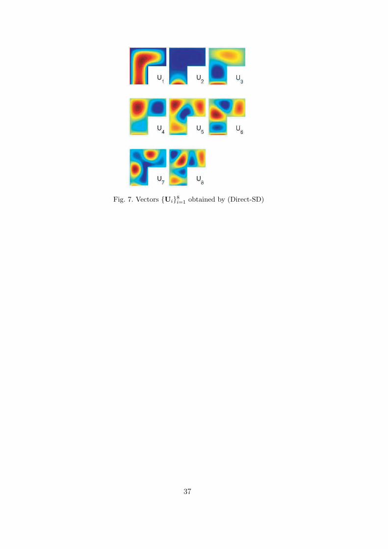
Fig. 7. Vectors Ui8i=1 obtained by (Direct-SD)

37

0 20 40 60 80 10010

−6

10−5

10−4

10−3

10−2

10−1

100

Time (s)

erro

r

P−GSDPU−GSDPCG

Fig. 8. Error εsol versus computation time for algorithms (P-GSD), (PU-GSD) and(PCG)

38

1 1.5 2 2.5 310

−20

10−15

10−10

10−5

100

order M

erro

r


Fig. 9. Error in A-norm with respect to the order of decomposition M for (P-GSD),(PU-GSD) and (Direct-SD)

39

1 1.2 1.4 1.6 1.8 210

−15

10−10

10−5

100

order M

erro

r

γstop

=0.5, kmax

=∞

γstop

=0.1, kmax

=∞

γstop

=0.01, kmax

=∞

γstop

=0.001, kmax

=∞

(a) Influence of γstop

1 1.2 1.4 1.6 1.8 210

−15

10−10

10−5

100

order M

erro

r

γstop

=0.05, kmax

=1

γstop

=0.05, kmax

=2

γstop

=0.05, kmax

=3

γstop

=0.05, kmax

=4

(b) Influence of kmax

Fig. 10. Relative error with respect to the order of decomposition M for (P-GSD).Influence of parameters γstop (a) and kmax (b)

40

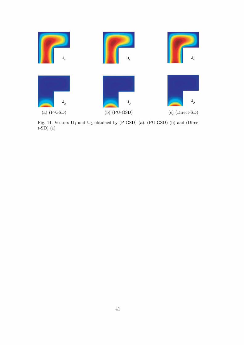
(a) (P-GSD) (b) (PU-GSD) (c) (Direct-SD)

Fig. 11. Vectors U1 and U2 obtained by (P-GSD) (a), (PU-GSD) (b) and (Direc-t-SD) (c)

41

−0.6 −0.4 −0.2 0 0.2 0.4 0.6 0.8 10

0.5

1

1.5

2

2.5

3

3.5

4

4.5

pdf(λ1)

pdf(λ2)

Fig. 12. Probability density functions of λ1 and λ2

42

−0.2 0 0.2 0.4 0.6 0.8 1

−0.5

−0.3

−0.1

0.1

0.3

0.5

λ1

λ 2

Fig. 13. Joint probability density function of λ1 and λ2

43

1 2 3 4 5 6 7 810

−4

10−3

10−2

10−1

100

order M

erro

r


(a) εsol

1 2 3 4 5 6 7 810

−3

10−2

10−1

100

order M

erro

r


(b) εsol,A

Fig. 14. Relative error with respect to the order of decomposition M for (P-GSD),(PU-GSD) and (Direct-SD). (a) L2-norm, (b) A-norm

44

(a) (P-GSD) (b) (PU-GSD)

Fig. 15. Vectors Ui8i=1 obtained by (P-GSD) (a) and (PU-GSD) (b)

45

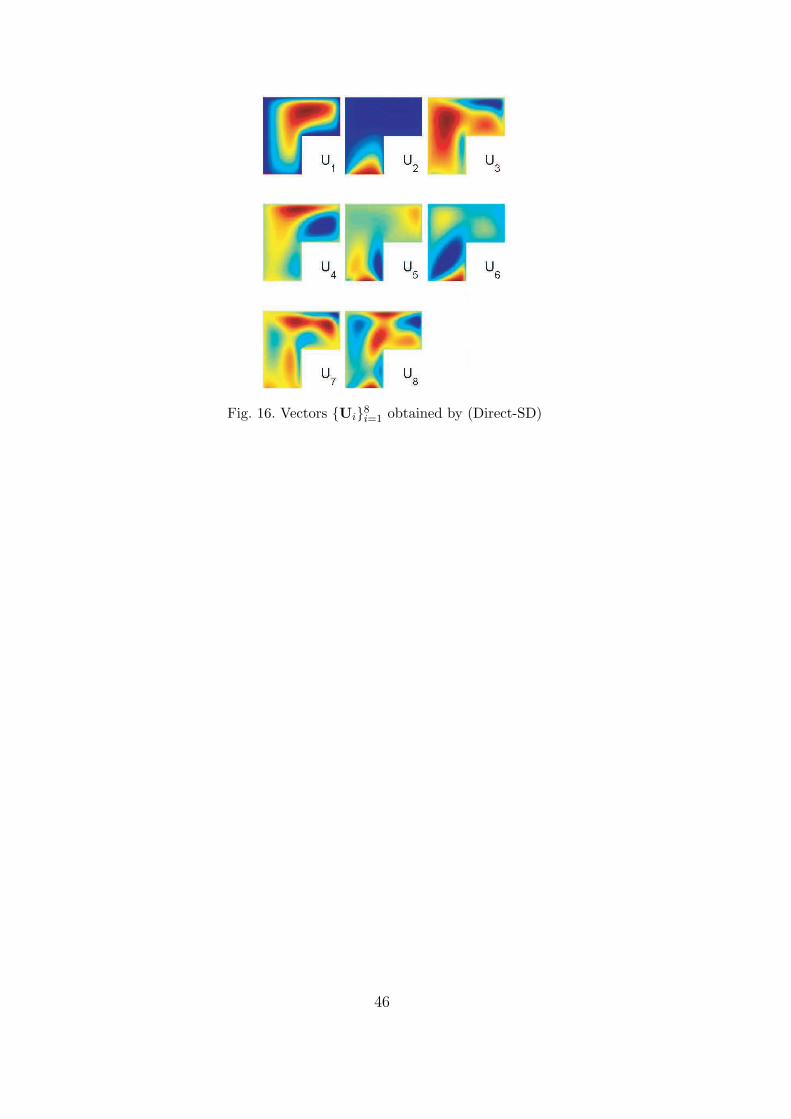
Fig. 16. Vectors Ui8i=1 obtained by (Direct-SD)

46

a generalized spectral decomposition technique to … · a generalized spectral decomposition...

Documents