species distribution modelling for plant communities

Species distribution modelling for plant communities: stacked single species or multivariate modelling approaches?

Henderson, E. B., Ohmann, J. L., Gregory, M. J., Roberts, H. M., Zald, H. (2014), Species distribution modelling for plant communities: stacked single species or multivariate modelling approaches?. Applied Vegetation Science, 17: 516–527. doi:10.1111/avsc.12085

10.1111/avsc.12085

John Wiley & Sons Ltd.

Version of Record

http://cdss.library.oregonstate.edu/sa-termsofuse

http://survey.az1.qualtrics.com/SE/?SID=SV_8Io4d9aAYR1VgGx

http://cdss.library.oregonstate.edu/sa-termsofuse

Applied Vegetation Science 17 (2014) 516–527

Species distributionmodelling for plant communities:stacked single species or multivariatemodellingapproaches?

Emilie B. Henderson, Janet L. Ohmann, Matthew J. Gregory, Heather M. Roberts & HaroldZald

Keywords

Nearest-neighbor imputation; Plant community

composition; Random forest; Species

distribution modelling; Vegetationmapping;

Western Oregon

Nomenclature

USDA NRCS (2000)

Received 21March 2013

Accepted 14 November 2013

Co-ordinating Editor: Sarah Goslee

Henderson, E.B. (corresponding author,

[email protected]): Institute

for Natural Resources, Oregon State

University,PO Box 751, Portland, OR, 97207-

0751, USA

Ohmann, J.L. (janet.ohmann@

oregonstate.edu): Pacific Northwest Research

Station, USDA Forest Service,3200 SW

JeffersonWay, Corvallis, OR, 97331, USA

Gregory, M.J. (matt.gregory@oregonstate.

edu), Roberts, H.M. (heather.roberts@

oregonstate.edu) & Zald, H. (harold.zald@

oregonstate.edu): Department of Forest

Ecosystems and Society, Oregon State

University, 321 Richardson Hall, Corvallis, OR,

97331, USA

Abstract

Aim: Landscape management and conservation planning require maps of vege-

tation composition and structure over large regions. Species distribution models

(SDMs) are often used for individual species, but projects mapping multiple spe-

cies are rarer. We compare maps of plant community composition assembled by

stacking results from many SDMs with multivariate maps constructed using

nearest-neighbor imputation.

Location:Western Cascades ecoregion, Oregon and California, USA.

Methods: We mapped distributions and abundances of 28 tree species over

4,007,110 ha at 30-m resolution using three approaches: SDMs using machine

learning (random forest) to yield: (1) binary (RF_Bin); (2) basal area (abun-

dance; RF_Abund) predictions; and (3) multi-species basal area predictions

using a nearest-neighbor imputation variant based on random forest (RF_NN).

We evaluated accuracy of binary predictions for all models, compared area

mapped with plot-based areal estimates, assessed species abundance at two spa-

tial scales and evaluated communities for species richness, problematic composi-

tional errors and overall community composition.

Results: RF_Bin yielded the strongest binary predictions (median True Skill

Statistics; RF_Bin: 0.57, RF_NN: 0.38, RF_Abund: 0.27). Plot-scale predic-

tions of abundance were poor for RF_Abund and RF_NN (median Agree-

ment Coefficient (AC): �1.77 and �2.28), but strong when summarized

over 50-km radius tessellated hexagons (median AC for both: 0.79). RF_A-

bund’s strength with abundance and weakness with binary predictions

stems from predicting small values instead of zeros. The number of zero

value predictions from RF_NN was closest to counts of zeros in the plot

data. Correspondingly, RF_NN’s map-based species area estimates closely

matched plot-based area estimates. RF_NN also performed best for commu-

nity-level accuracy metrics.

Conclusions: RF_NN was the best technique for building a broad-scale map

of diversity and composition because the modelling framework maintained

inter-species relationships from the input plot data. Re-assembling communi-

ties from single variable maps often yielded unrealistic communities.

Although RF_NN rarely excelled at single species predictions of presence or

abundance, it was often adequate to many (but not all) applications in both

dimensions. We discuss our results in the context of map utility for applica-

tions in the fields of ecology, conservation and natural resource manage-

ment planning. We highlight how RF_NN is well-suited for mapping current

but not future vegetation.

Applied Vegetation Science516 Doi: 10.1111/avsc.12085© 2014 International Association for Vegetation Science

Introduction

Maps of current vegetation are an essential component of

landscape management and conservation planning. Vege-

tation maps can be used to inform conservation strategies

(US Geological Survey 2011), understand the distribution

of invasive forest pathogens (V�aclav�ık et al. 2010) and ini-

tialize modelling efforts that explore how the future might

look in the context of human management and climate

change (e.g. Scheller & Mladenoff 2004; Hemstrom et al.

2007).

Species distribution modelling (SDM) techniques have

been widely used for mapping geographic ranges of com-

mon trees (e.g. Schroeder et al. 2010), rare species (e.g.

Engler et al. 2004) and species richness (e.g. Guisan &

Rahbek 2011). Projects mapping multiple species are less

common (but see Elith & Leathwick 2007; Baselga & Ara-

�ujo 2009; Ohmann et al. 2011; Wilson et al. 2012). There

is a strong focus in the SDM literature on mapping species

presences, perhaps a legacy of the abundant studies esti-

mating rare species’ habitat from presence-only data sets

(Newbold 2010). However, many applications require spe-

cies-specific information on presences and abundances as

well as community composition and diversity.

Stacking maps from individual species distribution mod-

els often yields problematic community-level results

because errors in each model are combined (Dubuis et al.

2011; Guisan & Rahbek 2011). These errors in single spe-

cies models result from a variety of factors. Species’ distri-

butions may not be in equilibrium with current climate

conditions (Elith et al. 2010). Presence (or abundance)

may be constrained by land-use and disturbance history

(e.g. Motzkin et al. 1996) as well as interspecific interac-

tions (e.g. Ettinger et al. 2011). SDMs often overestimate

species ranges because they tend to illustrate potential

rather than realized niches (Jim�enez-Valverde et al.

2008), perhaps because they are often unconstrained by

some of the above-mentioned factors due to lack of avail-

able data. The net effect of overestimating species pres-

ences is that stacked models yield inflated estimates of

species richness (Dubuis et al. 2011; Guisan & Rahbek

2011; Pottier et al. 2012), and predicted communities may

not reflect those that currently exist in nature (Baselga &

Ara�ujo 2010). Inaccurate compositional representation

renders maps less fit for some uses, such as designing

reserves that adequately represent biodiversity (Margules

& Pressey 2000). Community composition and species

richness estimates can be improved with additional layers

of analysis and information (e.g. Clark et al. 2011; Guisan

& Rahbek 2011). However, these extended analyses will

not be easy to accomplish across broad areas, with major

constraints to time, data and existing knowledge and

expertise.

We use the random forest machine learning algorithm,

a SDM technique that can yield strong results for mapping

individual species (Evans & Cushman 2009) and that has

grown in popularity in recent years (Cutler et al. 2007).

The random forest algorithm performs well for species dis-

tribution modelling for several reasons: (1) it is non-para-

metric, and hence flexible in terms of the explanatory

variables that it can handle; (2) it can represent non-linear

relationships between response and explanatory variables

and also hierarchical interactions of explanatory variables;

and (3) it uses information on species presence and

absence, a useful trait when complete data are available.

Of particular importance to our work here, the random

forest algorithm has been extended in utility to inform the

distance matrix used in nearest-neighbor imputation

(Crookston & Finley 2008), which can yield multivariate

predictions. Hence it is a useful technique for comparing

single species and multivariate approaches to mapping

communities.

Nearest-neighbor imputation techniques have been ris-

ing in popularity within the forestry community (Eskelson

et al. 2009), as forest management planning activities

often require multivariate maps describing forest structure

and composition. Imputation is defined as filling inmissing

values within a data set with known values from that same

data set. In our application, the ‘missing values’ are pixels

within a raster data set, and the known values come from

vegetation survey plot data. In our implementation, each

prediction is a link to a single plot. Therefore, model

predictions are constrained to communities represented

in the input plot data. This means that the net effects

of species interactions and site history on community

structure are preserved from the original plot data.

Imputation mapping can be viewed as an extension to

Ferrier & Guisan’s (2006) third approach for commu-

nity-level mapping: rather than ‘assemble and predict

together’, it could be called ‘no assembly necessary,

simply predict together’.

In this paper, we explore the trade-offs and conse-

quences that are inherent in two approaches: mapping

plant communities as cohesive units or stacking single spe-

cies models. We compare results built through single spe-

cies random forest models (stacked models of presence

and abundance, hereafter referred to as RF_Bin and

RF_Abund) with those generated by random forest-

based nearest-neighbor imputation (community-level

mapping, hereafter referred to as RF_NN). We test the

hypothesis that nearest-neighbor imputation mapping

can yield solid predictions for many dimensions of plant

community composition, even though single species

models may out-perform imputation in a single dimen-

sion at a time.

517Applied Vegetation ScienceDoi: 10.1111/avsc.12085© 2014 International Association for Vegetation Science

E.B. Henderson et al. Plant community distributionmodelling

Methods

Study area

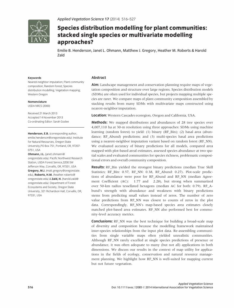
We built maps of forest composition across the Oregon

Western Cascades ecoregion (Fig. 1). The forested area

encompasses 4,007,110 ha and stretches from the Wash-

ington state border at its northern end into northern Cali-

fornia at its southern end. The vegetation of the region

varies along three primary gradients: latitude, elevation

and climate. Regional climate ranges from maritime in the

west to continental in the east (low seasonality to high sea-

sonality) and interacts with the elevation gradient (colder

temperatures and more snow at high elevations). Eleva-

tions modelled range from near sea level to upper tree line

(ca. 1500 m). The latitudinal gradient is biogeographic,

with elements of Alaskan flora in the north (e.g. Callitropsis

nootkatensis) and species that reach their peak in California

(e.g. Pinus lambertiana) in the south.

Data

We used 1948 US Forest Service Forest Inventory and

Analysis (FIA) annual plots, located within 10 km of the

study region (including plots within this 10 km buffer that

decrease edge effects). We summarized the basic FIA data

across whole plots, generating a matrix of basal area

(m2�ha�1) by species and plot. These survey plots contain

information on presence and absence as well as abun-

dance.

Our mapped explanatory variables were rasters (30-m

ground pixel resolution) encompassing five thematic areas:

(1) spectral reflectance (tasseled cap transformation of

Landsat imagery, brightness, greenness and wetness: Crist

& Cicone 1984); (2) climate (PRISM: Daly et al. 2008; 11

variables); (3) topography (elevation from the National

Elevation Dataset, and derivatives: Gesch et al. 2009; nine

variables); (4) soil parent material (mosaic of SSURGO: Soil

Survey Staff 2006 and the US Forest Service Soil Resources

Inventory; nine variables); and (5) location (latitude and

longitude). Details on each variable are available in the

online appendix (Appendix S1).

For mapping and modelling exercises where the most

accurate mapping of a single region is the primary goal,

attention to variable selection would be merited. However,

in our experience, model accuracy changes subtly with

variable reductions as long as the five thematic areas men-

tioned above are well represented. Also, random forest is

relatively robust to colinearity in explanatory variables.

Because of these two factors, and because model compari-

son was our primary purpose, we included all variables in

all models.

Modelling approach

We built maps of 28 tree species using three approaches,

all based on the random forest technique: (1) binary pre-

diction of presence/absence for each species independently

(28 total models, one for each species, approach referred to

as: RF_Bin); (2) continuous prediction of basal area

(m2�ha�1) for each species independently (28 total models,

approach referred to as: RF_Abund); and (3) continuous

prediction of basal area for all species simultaneously using

a random forest-based imputationmodel (onemultivariate

model: RF_NN). Basal area predictions from RF_NN and

RF_Abund were transformed to binary for comparison

with RF_Bin.

The random forest model builds on the functionality of

single classification trees (or regression trees for continu-

ous predictions) by extracting a single prediction from an

ensemble of tree models (we used 1000). Each individual

classification tree within a random forest is built from a

random subset of observations and explanatory variables

(Breiman 2001). We built RF_Bin and RF_Abund models

within the R environment for statistical computing (v

3.0.1; R Foundation for Statistical Computing, Vienna,

Austria), using the R-package ‘randomForest’ (Liaw &

Wiener 2002). For our binary model, predictions range

from 0 to 1 and reflect the proportion of classification trees

within the random forest predicting a given species to be

present rather than absent. We translate this continuous

Washington

Oregon

California

Nonforest (not mapped)Forest (mapped)Plot pool extent

0 140 28070 Kilometers

Cas

cade

Cre

st

Paci

fic O

cean

Fig. 1. Study area includes the forests of the Western Cascades

ecoregion, stretching from the northern Oregon border into northern

California. Plots used for modelling are drawn from the forested area

within the boundaries of a 10-km buffer around the ecoregion.


Plant community distribution modelling E.B. Henderson et al.

output to binary by applying a cut-off threshold. This

threshold was identified by the precision-recall F-measure

(Parviainen et al. 2008) using the R-package ‘rocr’ (Sing

et al. 2005) with an alpha value of 0.5 to balance the

weight of false positives and negatives. Predicted values

from our RF_Abund models were the average basal area

predicted by the regression trees within the random forest.

We also built RF_NN maps using the R-package ‘yaIm-

pute’ (Crookston & Finley 2008). The method imple-

mented in this R-package amalgamates multiple random

forest models, each tuned to a single response variable that

is a summary of species compositional data (we used three:

dominant species, basal area of the dominant species, total

basal area). To generate predictions, RF_NN chooses neigh-

bor plots based on a non-Euclidean distance measure built

from the nodes matrix of the amalgamated random forest

models. This nodes matrix holds a plot identifier for each

terminus (or ‘leaf’) of each classification tree in the random

forest models. For new locations (map pixels), the terminal

nodes where the pixel falls in the random forest models

are recorded. The nearest-neighbor plot for the new pixel

is the most frequent plot within its set of nodes.

Mapping and accuracy assessment

Each model prediction was mapped with our in-house R-

package ‘SDMap’ (Henderson unpubl; available upon

request to first author). We calculated all accuracy assess-

ment statistics on cross-validated predictions (ten-fold).

For each species and modelling approach, we calculated

three binary accuracy assessment measures: sensitivity,

specificity and the true skill statistic (TSS; Fielding & Bell

1997). We defined binary model success, for each metric,

as a value of 0.3. We also assessed the area occupied by

each species in the projected map surfaces. We estimated

actual areas of species distributions from FIA annual plots,

which are a systematic sample of the landscape. We calcu-

lated 95% confidence intervals for those area estimates

based on a binomial distribution (‘binom.confint’ function

in R-package ‘binom’).

We assessed the accuracy of continuous predictions

through the protocol outlined in Riemann et al. (2010).

The first half of that protocol uses three metrics of agree-

ment (described in Ji & Gallo 2006): (1) an overall agree-

ment coefficient (AC); (2) a measure of systematic

agreement (AC.sys); and (3) a measure of unsystematic

agreement (AC.uns). For each of these metrics, values

approaching or less than zero indicate no agreement while

values approaching one indicate strong agreement

between observations and predictions. We also plotted

empirical cumulative distribution functions (ECDF) for

observations and predictions, and calculated the Kolmogo-

rov–Smirnof statistic: the maximum distance between two

ECDF curves (K-S; Massey 1951). All of the continuous

accuracy metrics were calculated at two scales: (1) the plot

scale and (2) average values for plots falling within tessel-

lated hexagons across the study area (centers spaced

50 km apart: 9128 ha, each containing 44 FIA annual

plots on average).

We assessed several measures of accuracy related to

community composition. For RF_Bin and RF_Abund, we

developed community matrices by combining predictions

from each individual species model into a single matrix,

with rows for plots and columns for species. Post-model-

ling aggregation was unnecessary for RF_NN since predic-

tions were generated for all species simultaneously. We

compared observed and predicted species richness at the

plot locations with a generalized linear model (Poisson

family, with a log link function). We determined the prev-

alence of problematic types of compositional accuracy, cal-

culating how frequently species that rarely co-occur

within our plot sample co-occur within our predicted spe-

cies matrix. We also calculated compositional distance

between observed and predicted communities at each plot:

Sørenson distance on binary matrices and Bray–Curtis dis-

tance on abundance matrices using the ‘vegdist’ function

in the R-package ‘vegan’. We illustrate distributions of

these distances with ECDF plots.

Results

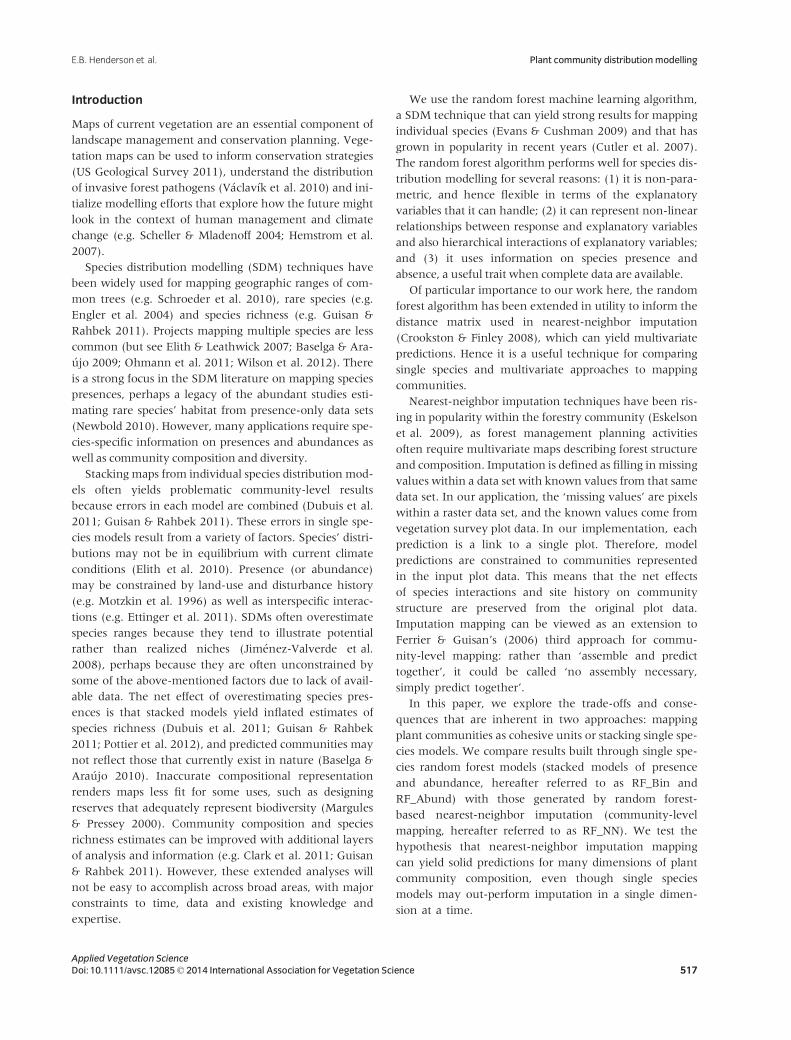
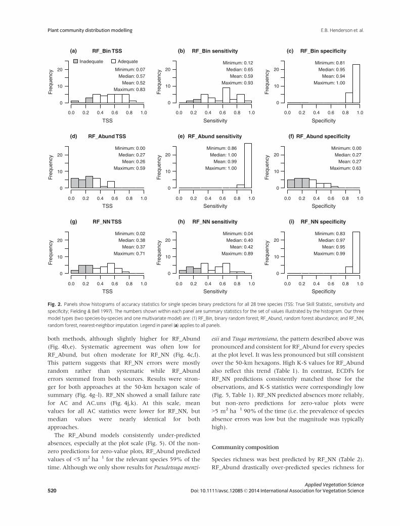
Single species predictions – binary

The RF_Bin models were strongest in differentiating spe-

cies presence and absence, combining strong sensitivity

with outstanding specificity to yield generally strong TSS

statistics and an 86% success rate (Fig. 2a–c). RF_Abund

often yielded predictions with high sensitivity, low speci-

ficity and poor TSS and a success rate of just 43% (Fig. 2b–

d). The RF_NN model showed moderate sensitivity, high

specificity andmoderate TSS (Fig. 2d–f) as well as an inter-

mediate success rate (64%).

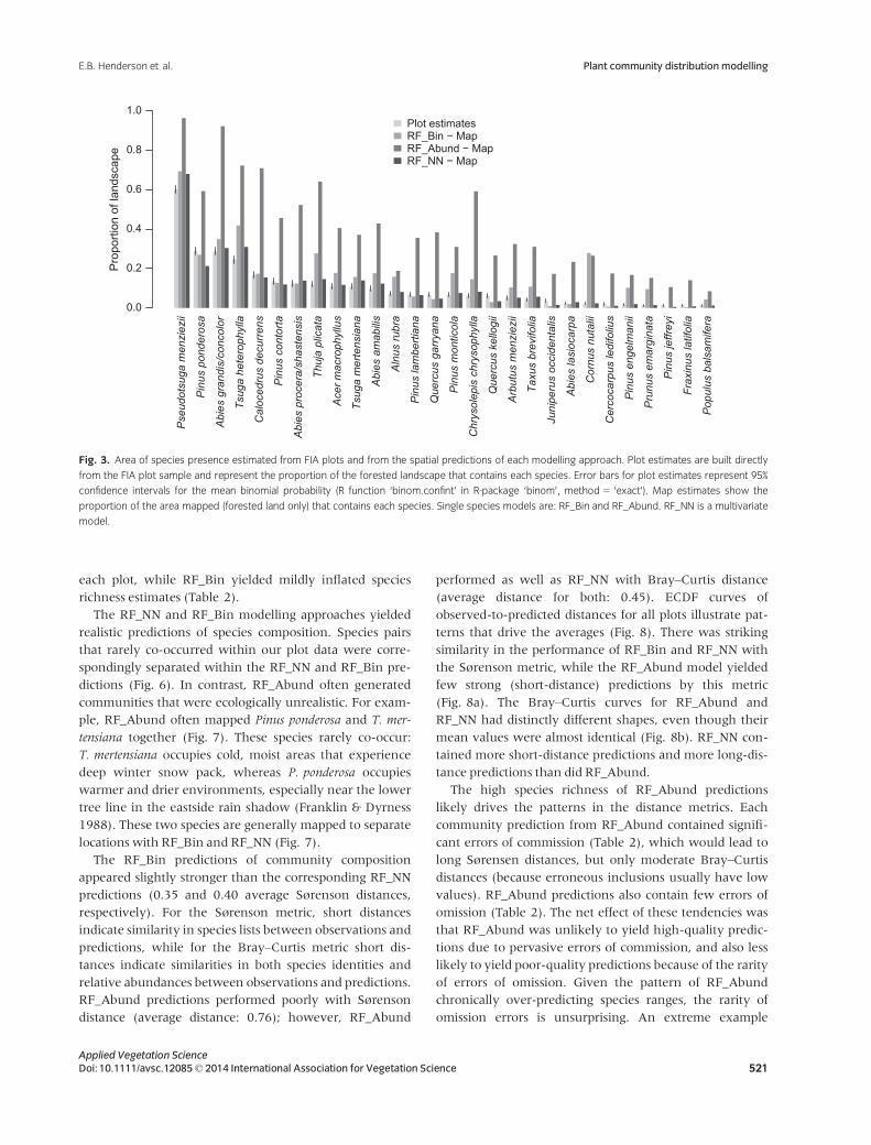
These differences in sensitivity and specificity were

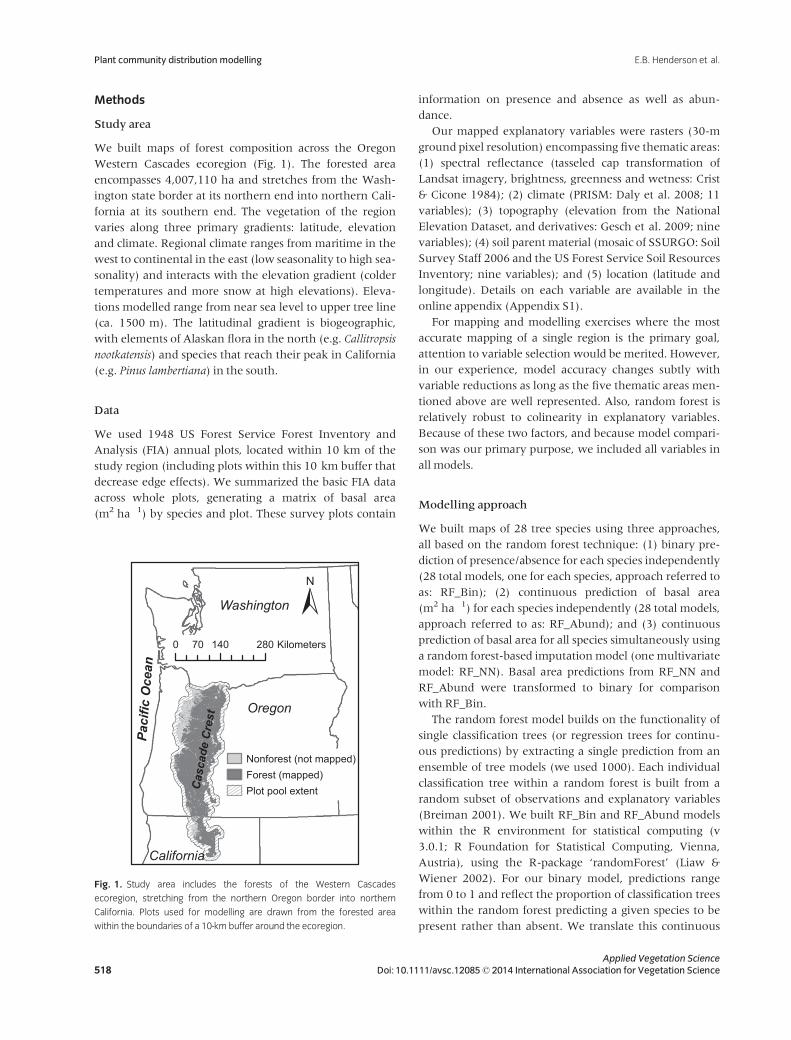
expressed in the maps. Models with high sensitivity and

low specificity (most of the RF_Abund models) drastically

over-mapped species presence, while mapped estimates of

species areas from RF_NN aligned well with plot-based

estimates of area (Fig. 3). Because TSSswere generally rea-

sonable for RF_NN (Fig. 2), we concluded that this area

was mapped to reasonable locations as well as having the

correct spatial extent.

Single species predictions – abundance

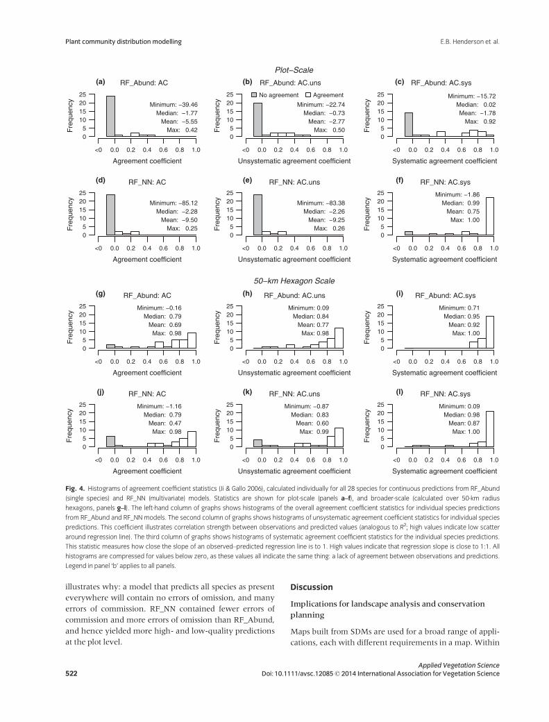
We found significant errors in abundance predictions at

the plot scale for RF_Abund and RF_NN (Fig. 4a,d). At the

plot level, unsystematic agreement was generally low for



both methods, although slightly higher for RF_Abund

(Fig. 4b,e). Systematic agreement was often low for

RF_Abund, but often moderate for RF_NN (Fig. 4c,f).

This pattern suggests that RF_NN errors were mostly

random rather than systematic while RF_Abund

errors stemmed from both sources. Results were stron-

ger for both approaches at the 50-km hexagon scale of

summary (Fig. 4g–l). RF_NN showed a small failure rate

for AC and AC.uns (Fig. 4j,k). At this scale, mean

values for all AC statistics were lower for RF_NN, but

median values were nearly identical for both

approaches.

The RF_Abund models consistently under-predicted

absences, especially at the plot scale (Fig. 5). Of the non-

zero predictions for zero-value plots, RF_Abund predicted

values of <5 m2�ha�1 for the relevant species 59% of the

time. Although we only show results for Pseudotsuga menzi-

esii and Tsuga mertensiana, the pattern described above was

pronounced and consistent for RF_Abund for every species

at the plot level. It was less pronounced but still consistent

over the 50-km hexagons. High K-S values for RF_Abund

also reflect this trend (Table 1). In contrast, ECDFs for

RF_NN predictions consistently matched those for the

observations, and K-S statistics were correspondingly low

(Fig. 5, Table 1). RF_NN predicted absences more reliably,

but non-zero predictions for zero-value plots were

>5 m2�ha�1 90% of the time (i.e. the prevalence of species

absence errors was low but the magnitude was typically

high).

Community composition

Species richness was best predicted by RF_NN (Table 2).

RF_Abund drastically over-predicted species richness for

0.0 0.2 0.4 0.6 0.8 1.0

0

10

20

TSS

Freq

uenc

yRF_Bin TSS

Minimum: 0.07Median: 0.57

Mean: 0.52Maximum: 0.83

Inadequate Adequate

(a)

0.0 0.2 0.4 0.6 0.8 1.0

0

10

20

TSS

Freq

uenc

y

RF_Abund TSS



(d)

0.0 0.2 0.4 0.6 0.8 1.0

0

10

20

TSS

Freq

uenc

y

RF_NN TSS



(g)

0.0 0.2 0.4 0.6 0.8 1.0

0

10

20

Sensitivity

Freq

uenc

y

RF_Bin sensitivity



(b)

0.0 0.2 0.4 0.6 0.8 1.0

0

10

20

Sensitivity

Freq

uenc

y

RF_Abund sensitivity



(e)

0.0 0.2 0.4 0.6 0.8 1.0

0

10

20

Sensitivity

Freq

uenc

y

RF_NN sensitivity



(h)

0.0 0.2 0.4 0.6 0.8 1.0

0

10

20

Specificity

Freq

uenc

y

RF_Bin specificity



(c)

0.0 0.2 0.4 0.6 0.8 1.0

0

10

20

Specificity

Freq

uenc

y

RF_Abund specificity



(f)

0.0 0.2 0.4 0.6 0.8 1.0

0

10

20

Specificity

Freq

uenc

y

RF_NN specificity



(i)

Fig. 2. Panels show histograms of accuracy statistics for single species binary predictions for all 28 tree species (TSS: True Skill Statistic, sensitivity and

specificity; Fielding & Bell 1997). The numbers shown within each panel are summary statistics for the set of values illustrated by the histogram. Our three

model types (two species-by-species and one multivariate model) are: (1) RF_Bin, binary random forest; RF_Abund, random forest abundance; and RF_NN,

random forest, nearest-neighbor imputation. Legend in panel (a) applies to all panels.



each plot, while RF_Bin yielded mildly inflated species

richness estimates (Table 2).

The RF_NN and RF_Bin modelling approaches yielded

realistic predictions of species composition. Species pairs

that rarely co-occurred within our plot data were corre-

spondingly separated within the RF_NN and RF_Bin pre-

dictions (Fig. 6). In contrast, RF_Abund often generated

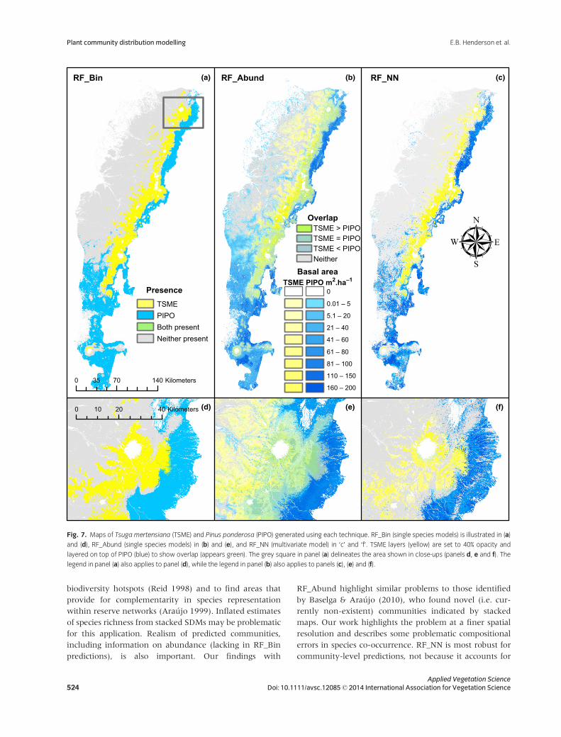
communities that were ecologically unrealistic. For exam-

ple, RF_Abund often mapped Pinus ponderosa and T. mer-

tensiana together (Fig. 7). These species rarely co-occur:

T. mertensiana occupies cold, moist areas that experience

deep winter snow pack, whereas P. ponderosa occupies

warmer and drier environments, especially near the lower

tree line in the eastside rain shadow (Franklin & Dyrness

1988). These two species are generally mapped to separate

locations with RF_Bin and RF_NN (Fig. 7).

The RF_Bin predictions of community composition

appeared slightly stronger than the corresponding RF_NN

predictions (0.35 and 0.40 average Sørenson distances,

respectively). For the Sørenson metric, short distances

indicate similarity in species lists between observations and

predictions, while for the Bray–Curtis metric short dis-

tances indicate similarities in both species identities and

relative abundances between observations and predictions.

RF_Abund predictions performed poorly with Sørenson

distance (average distance: 0.76); however, RF_Abund

performed as well as RF_NN with Bray–Curtis distance

(average distance for both: 0.45). ECDF curves of

observed-to-predicted distances for all plots illustrate pat-

terns that drive the averages (Fig. 8). There was striking

similarity in the performance of RF_Bin and RF_NN with

the Sørenson metric, while the RF_Abund model yielded

few strong (short-distance) predictions by this metric

(Fig. 8a). The Bray–Curtis curves for RF_Abund and

RF_NN had distinctly different shapes, even though their

mean values were almost identical (Fig. 8b). RF_NN con-

tained more short-distance predictions and more long-dis-

tance predictions than did RF_Abund.

The high species richness of RF_Abund predictions

likely drives the patterns in the distance metrics. Each

community prediction from RF_Abund contained signifi-

cant errors of commission (Table 2), which would lead to

long Sørensen distances, but only moderate Bray–Curtis

distances (because erroneous inclusions usually have low

values). RF_Abund predictions also contain few errors of

omission (Table 2). The net effect of these tendencies was

that RF_Abund was unlikely to yield high-quality predic-

tions due to pervasive errors of commission, and also less

likely to yield poor-quality predictions because of the rarity

of errors of omission. Given the pattern of RF_Abund

chronically over-predicting species ranges, the rarity of

omission errors is unsurprising. An extreme example

Plot estimatesRF_Bin − MapRF_Abund − MapRF_NN − Map

Pro

porti

on o

f lan

dsca

pe

Pse

udot

suga

men

ziez

ii

Pin

us p

onde

rosa

Abi

es g

rand

is/c

onco

lor

Tsug

a he

tero

phyl

la

Cal

oced

rus

decu

rren

s

Pin

us c

onto

rta

Abi

es p

roce

ra/s

hast

ensi

s

Thuj

a pl

icat

a

Ace

r mac

roph

yllu

s

Tsug

a m

erte

nsia

na

Abi

es a

mab

ilis

Aln

us ru

bra

Pin

us la

mbe

rtian

a

Que

rcus

gar

ryan

a

Pin

us m

ontic

ola

Chr

ysol

epis

chr

ysop

hylla

Que

rcus

kel

logi

i

Arb

utus

men

ziez

ii

Taxu

s br

evifo

lia

Juni

peru

s oc

cide

ntal

is

Abi

es la

sioc

arpa

Cor

nus

nuta

lii

Cer

coca

rpus

ledi

foliu

s

Pin

us e

ngel

man

ii

Pru

nus

emar

gina

ta

Pin

us je

ffrey

i

Frax

inus

latif

olia

Pop

ulus

bal

sam

ifera

0.0

0.2

0.4

0.6

0.8

1.0

Fig. 3. Area of species presence estimated from FIA plots and from the spatial predictions of each modelling approach. Plot estimates are built directly

from the FIA plot sample and represent the proportion of the forested landscape that contains each species. Error bars for plot estimates represent 95%

confidence intervals for the mean binomial probability (R function ‘binom.confint’ in R-package ‘binom’, method = ‘exact’). Map estimates show the

proportion of the area mapped (forested land only) that contains each species. Single species models are: RF_Bin and RF_Abund. RF_NN is a multivariate

model.



illustrates why: a model that predicts all species as present

everywhere will contain no errors of omission, and many

errors of commission. RF_NN contained fewer errors of

commission and more errors of omission than RF_Abund,

and hence yielded more high- and low-quality predictions

at the plot level.

Discussion

Implications for landscape analysis and conservation

planning

Maps built from SDMs are used for a broad range of appli-

cations, each with different requirements in a map.Within

RF_Abund: AC

Agreement coefficient

<0 0.0 0.2 0.4 0.6 0.8 1.0

05

10152025

Fre

quen

cy Minimum: −39.46Median: −1.77

Mean: −5.55Max: 0.42

(a) RF_Abund: AC.uns

Unsystematic agreement coefficient

<0 0.0 0.2 0.4 0.6 0.8 1.0

05

10152025

Fre

quen


Mean: −2.77Max: 0.50

No agreement Agreement

(b) RF_Abund: AC.sys

Systematic agreement coefficient

<0 0.0 0.2 0.4 0.6 0.8 1.0

05

10152025

Fre

quen

cy

Minimum: −15.72Median: 0.02Mean: −1.78

Max: 0.92

(c)

RF_NN: AC


<0 0.0 0.2 0.4 0.6 0.8 1.0

05

10152025

Fre

quen


Mean: −9.50Max: 0.25

(d) RF_NN: AC.uns


<0 0.0 0.2 0.4 0.6 0.8 1.0

05

10152025

Fre

quen


Mean: −9.25Max: 0.26

(e) RF_NN: AC.sys


<0 0.0 0.2 0.4 0.6 0.8 1.0

05

10152025

Fre

quen

cy

Minimum: −1.86Median: 0.99

Mean: 0.75Max: 1.00

(f)

RF_Abund: AC


<0 0.0 0.2 0.4 0.6 0.8 1.0

05

10152025

Fre

quen

cy


Mean: 0.69Max: 0.98

(g) RF_Abund: AC.uns


<0 0.0 0.2 0.4 0.6 0.8 1.0

05

10152025

Fre

quen

cy


Mean: 0.77Max: 0.98

(h) RF_Abund: AC.sys


<0 0.0 0.2 0.4 0.6 0.8 1.0

05

10152025

Fre

quen

cy


Mean: 0.92Max: 1.00

(i)

RF_NN: AC


<0 0.0 0.2 0.4 0.6 0.8 1.0

05

10152025

Fre

quen

cy


Mean: 0.47Max: 0.98

(j) RF_NN: AC.uns


<0 0.0 0.2 0.4 0.6 0.8 1.0

05

10152025

Fre

quen

cy


Mean: 0.60Max: 0.99

(k) RF_NN: AC.sys


<0 0.0 0.2 0.4 0.6 0.8 1.0

05

10152025

Fre

quen

cy


Mean: 0.87Max: 1.00

(l)

Plot−Scale

50−km Hexagon Scale

Fig. 4. Histograms of agreement coefficient statistics (Ji & Gallo 2006), calculated individually for all 28 species for continuous predictions from RF_Abund

(single species) and RF_NN (multivariate) models. Statistics are shown for plot-scale (panels a–f), and broader-scale (calculated over 50-km radius

hexagons, panels g–l). The left-hand column of graphs shows histograms of the overall agreement coefficient statistics for individual species predictions

from RF_Abund and RF_NNmodels. The second column of graphs shows histograms of unsystematic agreement coefficient statistics for individual species

predictions. This coefficient illustrates correlation strength between observations and predicted values (analogous to R2; high values indicate low scatter

around regression line). The third column of graphs shows histograms of systematic agreement coefficient statistics for the individual species predictions.

This statistic measures how close the slope of an observed–predicted regression line is to 1. High values indicate that regression slope is close to 1:1. All

histograms are compressed for values below zero, as these values all indicate the same thing: a lack of agreement between observations and predictions.

Legend in panel ‘b’ applies to all panels.



the field of conservation planning, fine and coarse filter

applications (Noss 1987) have distinctly different needs in

terms of map performance. Forestry applications require

unbiased multivariate information on forest composition

and structure (Eskelson et al. 2009). Ecological studies of

invasive pests may require information on many species

simultaneously (e.g. V�aclav�ık et al. 2010). Simulation

models often need input information on community com-

position, species abundances, as well as vegetation struc-

ture (e.g. Scheller & Mladenoff 2004; Hemstrom et al.

2007). Our maps have differing strengths and weaknesses,

and none is clearly ‘best’ for all applications. Here, we

highlight some of the trade-offs inherent in different con-

servation applications, and also place our work in the con-

text of estimating future vegetation under climate change.

For fine filter conservation focused on individual spe-

cies, our RF_Bin approach had clear advantages. This find-

ing was not surprising as random forest often performs

well in comparison with other techniques for building sin-

gle species binary maps (e.g. Marmion et al. 2009).

Although we have not modelled any threatened or endan-

gered species, the trade-offs we highlight are relevant to

that application. In particular, the balance between sensi-

tivity and specificity has important implications for map

utility (Loiselle et al. 2003). Conservation or development

plans formulated from low-sensitivity maps may fail to

protect missed populations, placing rare species at risk. On

the other hand, low-specificity maps may trigger costly

and unnecessary surveys.

For coarse filter conservation, RF_NN is well suited.

Community-level information is needed to identify

Pseudotsuga menziesii Tsuga mertensiana

Plot−scale

0 50 100 2000.0

0.2

0.4

0.6

0.8

1.0

m2.ha–1 m2.ha–1

m2.ha–1 m2.ha–1

Cum

ulat

ive

prop

ortio

n (a) (b)

(c) (d)

PlotsRF_AbundRF_NN

0 50 100 150 2000.0

0.2

0.4

0.6

0.8

1.0

50 km hexagon scale

0 40 80 1200.0

0.2

0.4

0.6

0.8

1.0

Cum

ulat

ive

prop

ortio

n

0 10 20 30 40 500.0

0.2

0.4

0.6

0.8

1.0

Fig. 5. Empirical cumulative distribution functions for observations (plots)

and spatial predictions of P. menziezii and Tsuga mertensiana basal area,

from RF_Abund (single species) and RF_NN (multivariate) models, at the

plot scale (a, b), and summarized for all plots within 50-km hexagons (c, d).

Legend in panel ‘a’ applies to all panels.

AB

AM

_AR

ME

AB

AM

_PIP

O

ALR

U2_

PIP

O

ALR

U2_

TS

ME

AR

ME

_TS

ME

PIP

O_T

SM

E

Co−

occu

rren

cepr

opor

tion

of r

ange

0.0

0.1

0.2

0.3

0.4

0.5Plot estimateRF_Abund − MapRF_Bin − MapRF_NN − Map

Fig. 6. Species pair co-occurrences in plot data and spatial predictions.

This graph shows the range overlap of six species pairs, expressed as a

proportion of the total joint range for both species (e.g. for the area

occupied by either ABAM or ARME in the RF_Abund map, they co-occur

over 12% of that area). These pairs were chosen from a pool of common

species to represent species that rarely co-occur within the plot data. Pairs

are described by USDA Plants codes for species. ABAM, Abies amabilis;

ALRU2, Alnus rubra; ARME, Arbutus menziesii; PIPO, Pinus ponderosa;

TSME, Tsuga mertensiana. Single species models are: RF_Bin and

RF_Abund. RF_NN is a multivariate model.

Table 1. Kolmogorov–Smirnov test statistics comparing the distribution

of observed and predicted values for each species. Summaries presented

here are for all species at two scales of summary: plot level and within the

50-km hexagons. RF_Abund is a single species model. RF_NN is a multivari-

ate model.

Min. Mean Max.

RF_Abund– Plot 0.37 0.64 0.88

RF_NN– Plot 0.00 0.01 0.04

RF_Abund– Hex 0.11 0.51 0.84

RF_NN– Hex 0.05 0.10 0.19

Table 2. Average plot-level species richness and types of error in plot-

level species lists by model type. Values represent the average number of

species per plot. For each column, letter labels indicate which values are

significantly different from the others according to a generalized linear

model (alpha < 0.01). Within a column, cells with different letters are sta-

tistically different. Single species models are: RF_Bin and RF_Abund.

RF_NN is a multivariate model.

Species richness Omissions Commissions

RF_Bin 3.83 b 0.72 b 1.58 b

RF_Abund 21.51 c 0.01 a 18.54 c

RF_NN 2.89 a 1.19 c 1.10 a

Plots 2.98 a NA NA



biodiversity hotspots (Reid 1998) and to find areas that

provide for complementarity in species representation

within reserve networks (Ara�ujo 1999). Inflated estimates

of species richness from stacked SDMs may be problematic

for this application. Realism of predicted communities,

including information on abundance (lacking in RF_Bin

predictions), is also important. Our findings with

RF_Abund highlight similar problems to those identified

by Baselga & Ara�ujo (2010), who found novel (i.e. cur-

rently non-existent) communities indicated by stacked

maps. Our work highlights the problem at a finer spatial

resolution and describes some problematic compositional

errors in species co-occurrence. RF_NN is most robust for

community-level predictions, not because it accounts for

(a) (b) (c)

(d) (e) (f)

RF_Bin RF_Abund RF_NN


PresenceTSMEPIPOBoth presentNeither present


TSME PIPO m2.ha–1Basal area

Overlap

TSME = PIPOTSME > PIPO

TSME < PIPO

0

0.01 – 5

5.1 – 20

21 – 40

41 – 60

61 – 80

81 – 100

110 – 150

160 – 200

Neither

Fig. 7. Maps of Tsuga mertensiana (TSME) and Pinus ponderosa (PIPO) generated using each technique. RF_Bin (single species models) is illustrated in (a)

and (d), RF_Abund (single species models) in (b) and (e), and RF_NN (multivariate model) in ‘c’ and ‘f’. TSME layers (yellow) are set to 40% opacity and

layered on top of PIPO (blue) to show overlap (appears green). The grey square in panel (a) delineates the area shown in close-ups (panels d, e and f). The

legend in panel (a) also applies to panel (d), while the legend in panel (b) also applies to panels (c), (e) and (f).



the species interactions that constrain distributions in nat-

ure, but because its predictions are constrained to assem-

blages that reflect the outcomes of those interactions as

they are represented within the input plot data. Put

another way, the RF_NN procedure does not build realistic

species assemblages, but rather refrains from dis-assem-

bling them in the first place.

The RF_NN approach to mapping is a poor choice for

estimating future communities for the same reason that it

is a good choice for estimating current communities.

Because it can only predict species assemblages that are

present within the input plot data, it cannot estimate the

novel combinations that will likely emerge as species

respond individualistically to climate change (Huntley

1991). Single species approaches still provide a better alter-

native (e.g. Iverson & Prasad 1998), although the problem

of inflated species richness in stacked models will remain

because species interactions will shape new communities

that emerge as climate shifts (Walther 2010). Alternative

strategies tomodelling communities (e.g. Clark et al. 2011;

Guisan & Rahbek 2011), or simulation modelling (e.g.

Scheller & Mladenoff 2004) may be more appropriate for

estimating future forest communities. For the latter,

RF_NNmaps are well suited to provide a starting point.

Conclusions

Single species distribution models often yielded stronger

predictions for individual species for either presence or

abundance, but rarely both. Imputation often yielded ade-

quate estimates of both while also providing high-quality,

community-level information on diversity and composi-

tion. Imputed multivariate maps are therefore adequate

for many purposes, from conservation reserve design to

regional forest management plans, to simulation model

initialization.

Acknowledgements

The ideas behind this paper stemmed from work con-

ducted for the Nationwide Forest Imputation Study (Na-

FIS), a collaboration between researchers at Oregon State

University, Michigan State University and the US Forest

Service (the Forest Health Technology Enterprise Team,

the Western Wildland Environmental Threat Assessment

Center, the Remote Sensing Applications Center, Forest

Inventory and Analysis, the Pacific Northwest Research

Station, and the Northern Research Station).

References

Ara�ujo, M.B. 1999. Distribution patterns of biodiversity and the

design of a representative reserve network in Portugal. Diver-

sity and Distributions 5: 151–163.

Baselga, A. & Ara�ujo, M.B. 2009. Individualistic vs community

modelling of species distributions under climate change.

Ecography 32: 55–65.

Baselga, A. & Ara�ujo, M.B. 2010. Do community-level models

describe community variation effectively? Journal of Biogeog-

raphy 37: 1842–1850.

Breiman, L. 2001. Random forests. Machine Learning 45:

5–32.

Clark, J.S., Bell, D.M., Hersh, M.H., Kwit, M.C., Moran, E., Salk,

C., Stine, A., Valle, D. & Zhu, K. 2011. Individual-scale varia-

tion, species-scale differences: inference needed to under-

stand diversity. Ecology Letters 14: 1273–1287.

Crist, E.P. & Cicone, R.C. 1984. Application of the Tasseled Cap

concept to simulated thematic mapper data (transformation

for MSS crop and soil imagery). Photogrammetric Engineering

and Remote Sensing 50: 343–352.

Crookston, N.L. & Finley, A.O. 2008. Yaimpute: an R package for

kNN imputation. Journal of Statistical Software 23: 1–11.

Cutler, D.R., Edwards, T.C., Beard, K.H., Cutler, A., Hess, K.T.,

Gibson, J. & Lawler, J.J. 2007. Random forests for classifica-

tion in ecology. Ecology 88: 2783–2792.

Daly, C., Halbleib, M., Smith, J.I., Gibson, W.P., Doggett, M.K.,

Taylor, G.H., Curtis, J. & Pasteris, P.P. 2008. Physiographical-

ly sensitive mapping of climatological temperature and pre-

cipitation across the conterminous United States.

International Journal of Climatology 28: 2031–2064.

Dubuis, A., Pottier, J., Rion, V., Pellissier, L., Theurillat, J.-P. &

Guisan, A. 2011. Predicting spatial patterns of plant species

richness: a comparison of direct macroecological and species

stacking modelling approaches. Diversity and Distributions 17:

1122–1131.

0.0 0.4 0.8

0.0

0.2

0.4

0.6

0.8

1.0

Binary

Sørensen

Cum

ulat

ive

% o

f dat

aset

(a) (b)

Abundance

Bray−Curtis

RF_BinRF_AbundRF_NN

0.0 0.4 0.8

Fig. 8. Empirical cumulative distribution functions for the multivariate

distance between observed and predicted communities by modelling

method. Models with more short observed–predicted distances have

stronger community-level predictions (greater similarity between

observed and predicted communities). Values for (a) are calculated as the

Sørenson distance, which is the binary equivalent of Bray–Curtis distance

(shown in panel b). Sørenson distance analyses community similarities

with respect to species presence/absences while Bray–Curtis distance also

accounts for abundance. Single species models are: RF_Bin and

RF_Abund. RF_NN is a multivariate model.



Elith, J. & Leathwick, J. 2007. Predicting species distributions

from museum and herbarium records using multiresponse

models fitted with multivariate adaptive regression splines.

Diversity and Distributions 13: 265–275.

Elith, J., Kearney, M. & Phillips, S. 2010. The art of modelling

range-shifting species. Methods in Ecology and Evolution 1:

330–342.

Engler, R., Guisan, A. & Rechsteiner, L. 2004. An improved

approach for predicting the distribution of rare and endan-

gered species from occurrence and pseudo-absence data.

Journal of Applied Ecology 41: 263–274.

Eskelson, B.N.I., Temesgen, H., Lemay, V., Barrett, T.M., Crook-

ston, N.L. & Hudak, A.T. 2009. The roles of nearest neighbor

methods in imputing missing data in forest inventory and

monitoring databases. Scandinavian Journal of Forest Research

24: 235–246.

Ettinger, A., Ford, K. & HilleRisLambers, J. 2011. Climate deter-

mines upper, but not lower, altitudinal range limits of Pacific

Northwest conifers. Ecology 92: 1323–1331.

Evans, J. & Cushman, S. 2009. Gradient modeling of conifer spe-

cies using random forests. Landscape Ecology 24: 673–683.

Ferrier, S. & Guisan, A. 2006. Spatial modelling of biodiversity at

the community level. Journal of Applied Ecology 43: 393–404.

Fielding, A.H. & Bell, J.F. 1997. A review of methods for the

assessment of prediction errors in conservation presence/

absencemodels. Environmental Conservation 24: 38–49.

Franklin, J.F. & Dyrness, C.T. 1988. Natural vegetation of Oregon

andWashington. Oregon State University Press, Corvallis, OR.

Gesch, D., Evans, G., Mauck, J., Hutchinson, J. & Carswell., W.J.

Jr. 2009. The national map – elevation. US Geological Sur-

vey. Available at: http://pubs.usgs.gov/fs/2009/3053/pdf/

fs2009_3053.pdf.

Guisan, A. & Rahbek, C. 2011. SESAM – a new framework inte-

grating macroecological and species distribution models for

predicting spatio-temporal patterns of species assemblages.

Journal of Biogeography 38: 1433–1444.

Hemstrom, M.A., Merzenich, J., Reger, A. & Wales, B. 2007.

Integrated analysis of landscape management scenarios

using state and transitionmodels in the upper Grande Ronde

River Subbasin, Oregon, USA. Landscape and Urban Planning

80: 198–211.

Huntley, B. 1991. How plants respond to climate change: migra-

tion rates, individualism and the consequences for plant

communities.Annals of Botany 67: 15–22.

Iverson, L.R. & Prasad, A.M. 1998. Predicting abundance of 80

tree species following climate change in the Eastern United

States. Ecological Monographs 68: 465–485.

Ji, L. & Gallo, K. 2006. An agreement coefficient for image com-

parison. Photogrammetric Engineering and Remote Sensing 72:

823–833.

Jim�enez-Valverde, A., Lobo, J.M. & Hortal, J. 2008. Not as good

as they seem: the importance of concepts in species distribu-

tionmodelling. Diversity and Distributions 14: 885–890.

Liaw, A. & Wiener, M. 2002. Classification and regression by

random Forest. R News 2: 18–22.

Loiselle, B.A., Howell, C.A., Graham, C.H., Goerck, J.M., Brooks,

T., Smith, K.G. & Williams, P.H. 2003. Avoiding pitfalls of

using species distribution models in conservation planning.

Conservation Biology 17: 1591–1600.

Margules, C.R. & Pressey, R.L. 2000. Systematic conservation

planning.Nature 405: 243–253.

Marmion, M., Parviainen, M., Luoto, M., Heikkinen, R.K. &

Thuiller, W. 2009. Evaluation of consensus methods in pre-

dictive species distribution modelling. Diversity and Distribu-

tions 15: 59–69.

Massey, F.J. 1951. The Kolmogorov–Smirnov test for goodness

of fit. Journal of the American Statistical Association 46: 68–78.

Motzkin, G., Foster, D., Allen, A., Harrod, J. & Boone, R. 1996.

Controlling site to evaluate history: vegetation patterns of a

New England sand plain. Ecological Monographs 66: 345–365.

Newbold, T. 2010. Applications and limitations of museum data

for conservation and ecology, with particular attention to

species distribution models. Progress in Physical Geography 34:

3–22.

Noss, R.F. 1987. From plant communities to landscapes in con-

servation inventories: a look at The Nature Conservancy

(USA). Biological Conservation 41: 11–37.

Ohmann, J.L., Gregory, M.J., Henderson, E.B. & Roberts, H.M.

2011. Mapping gradients of community composition with

nearest-neighbor imputation: extending plot data for land-

scape analysis. Journal of Vegetation Science 22: 660–676.

Parviainen, M., Luoto, M., Rytt€ari, T. & Heikkinen, R.K. 2008.

Modelling the occurrence of threatened plant species in taiga

landscapes: methodological and ecological perspectives. Jour-

nal of Biogeography 35: 1888–1905.

Pottier, J., Dubuis, A., Pellissier, L., Maiorano, L., Rossier, L.,

Randin, C.F., Vittoz, P. & Guisan, A. 2012. The accuracy of

plant assemblage prediction from species distribution models

varies along environmental gradients. Global Ecology and Bio-

geography 22: 52–63.

Reid, W.V. 1998. Biodiversity hotspots. Trends in Ecology & Evolu-

tion 13: 275–280.

Riemann, R., Wilson, B.T., Lister, A. & Parks, S. 2010. An effec-

tive assessment protocol for continuous geospatial datasets of

forest characteristics using USFS Forest Inventory and

Analysis (FIA) data. Remote Sensing of Environment 114:

2337–2352.

Scheller, R.M. & Mladenoff, D.J. 2004. A forest growth and bio-

mass module for a landscape simulation model, LANDIS:

design, validation, and application. Ecological Modelling 180:

211–229.

Schroeder, T.A., Hamann, A., Wang, T. & Coops, N.C. 2010.

Occurrence and dominance of six Pacific Northwest conifer

species. Journal of Vegetation Science 21: 586–596.

Sing, T., Sander, O., Beerenwinkel, N. & Lengauer, T. 2005.

ROCR: visualizing classifier performance in R. Bioinformatics

21: 3940–3941.

Soil Survey Staff, Soil Survey Geographic (SSURGO). 2006.

Database for Oregon, U.S. Department of Agriculture,

Natural Resources Conservation Service.



US Geological Survey, Gap Analysis Program (GAP). 2011.

National Land Cover, Version 2. Available at: http://gapanal-

ysis.usgs.gov/gaplandcover/.

V�aclav�ık, T., Kanaskie, A., Hansen, E.M., Ohmann, J.L. & Me-

entemeyer, R.K. 2010. Predicting potential and actual distri-

bution of sudden oak death in Oregon: prioritizing landscape

contexts for early detection and eradication of disease out-

breaks. Forest Ecology andManagement 260: 1026–1035.

Walther, G.-R. 2010. Community and ecosystem responses to

recent climate change. Philosophical Transactions of the Royal

Society B: Biological Sciences 365: 2019–2024.

Wilson, B.T., Lister, A.J. & Riemann, R.I. 2012. A nearest-neigh-

bor imputation approach to mapping tree species over large

areas using forest inventory plots and moderate resolution

raster data. Forest Ecology andManagement 271: 182–198.

Supporting Information

Additional supporting information may be found in the

online version of this article:

Appendix S1.Descriptions of explanatory variables for all

models.



species distribution modelling for plant communities

Documents