sources of growth with a new data set - conference-board.org · pdf filechinese economy in the...
TRANSCRIPT

EEccoonnoomm iiccss PPrrooggrraamm WWoorrkkiinngg PPaapp eerr SSeerr iieess
China’s Growth and Productivity
Performance Debate Revisited
- Accounting for China’s Sources of Growth
with a New Data Set
Harry X. Wu
Institu te of Economic Research, Hitotsubashi University, Tokyo
[email protected] .ac.jp
&
The Conference Board China Center, Beijing
harry.wu@conference-board .org
January 2014
EEPPWWPP ##1144 –– 0011
Economics Program
845 Third Avenue
New York, NY 10022-6679
Tel. 212-759-0900
www.conference-board .org/ economics

As of December 30, 2013 Page 1
CHINA’S GROWTH AND PRODUCTIVITY PERFORMANCE
DEBATE REVISITED*
- Accounting for China’s Sources of Growth with A New Data Set
Harry X. Wu
Institute of Economic Research, Hitotsubashi University, Tokyo
&
The Conference Board China Center, Beijing
ABSTRACT
This study explores problems with official Chinese economic data that are often
ignored or overlooked in existing academic studies. They include structural breaks in
employment statistics, implausibly high labor productivity figures relating to “non-
material” services, serious inconsistencies between output measures in industrial
statistics versus those in national accounts, as well as between volume movements and
changes in real values. There are also conceptual flaws in official measures of fixed-
asset investment and biases in the prices of the investment. Alternative adjustments
for these problems are the basis for the construction of a new set of data for the
aggregate economy and its five major sectors in 1949-2012. I find that the impact of
external shocks is more pronounced using my alternative GDP estimates than with
official estimates. Under the most reasonable scenarios, my estimates show that
China’s annual TFP growth is -0.5 percent for the planning period and 1.1 percent for
the post-reform period, much slower than the results based on unadjusted official data
which is 0.1 and 3.2 percent respectively. However, China’s best TFP growth post-
reform is found for 2001-07 by 4.1 percent per annum and poorest TFP performance
is found for 2008-12 by -0.8 percent. For most of the sub-periods defined, on average
the results are very sensitive to how GDP estimates are adjusted, followed by what
investment deflator is used. But it is less sensitive to how employment data are
adjusted and what depreciation rate is adopted.
Keywords: Gross value added; the Gerschenkron effect, numbers employed and
hours worked; physical capital stock; human capital stock; total factor productivity;
economic development and reform in China
JEL Classification: E10, E24, C82, O47
* Part of this research was conducted when I worked with the late Professor Angus Maddison in
2006-09 to update our earlier data work for reassessing China’s long-run economic performance.
Substantial revision to the earlier data work began with my interactions with The Conference Board to
improve the Chinese data in the TCB Total Economy Database. I am in debt to helpful comments and
suggestions from Angus Maddison, Bart van Ark, Kyoji Fukao, Alan Heston, Shi Li, Carlo Milana,
Marcel Timmer, Gaaitzen J. de Vries, Ximing Yue, Zhaoyong Zhang, as well as participants at the
2010 AEA Meetings and seminars and workshops at RIETI (Japan), GGDC at Groningen University,
University of Queensland, University of Western Australia, Birkbeck College at University of London,
CEPII (Paris), and OECD Development Center. I also thank Reiko Ashizawa, Vivian Chen and
Xiaoqin Li for timely assistance, and Esther Shea and Nicholas Wu for reading and editing the earlier
versions of the manuscript. I am solely responsible for remaining errors and omissions.
As of December 30, 2013 Page 2
1. INTRODUCTION
The quality of China’s post-reform growth has been the subject of heated debate
in literature. It draws significant attention whenever the China model of reform and
development is appraised or questioned. The center of the debate is whether China’s
growth over the reform period is significantly attributed to productivity growth or
mainly driven by factor accumulation. Unfortunately, although more and more studies
have participated in the debate in the past two decades, it has remained unsettled and
inconclusive.
Based on the estimates of total factor productivity (TFP) for the aggregate
Chinese economy in the literature, we may approximately categorize the existing
studies into two opposite camps: optimistic versus pessimistic.1 The “optimists” may
be represented by the most recent studies by Perkins and Rawski (2008) and Bosworth
and Collins (2008) both attributing over 40 percent of China’s post-reform growth to
TFP – that is, 3.8 percent of annual TFP growth for the period 1978-2005 in the
former study and 3.6 percent for 1978-2004 in the latter.2 The “pessimists” may be
represented by Young’s study (2003) which only estimates China’s TFP growth at 1.4
percent per year for the period 1978-1998. Since Young only covers the non-
agricultural economy, one may argue that his estimate for the TFP growth should have
been even slower if agriculture were included – that is, at best TFP contributed no
more than 15 percent of the growth in that period.3 There are, however, estimates
standing in between which includes an estimate of 2.4 percent of annual TFP growth
for the period 1978-1999 in Wang and Yao (2002) and 2.5 percent for 1982-2000 in
Cao et al. (2009).
1 For the purpose of this study, we mainly cover the estimates using the aggregate data unless
studies using regional and sectoral data that cover the whole economy, e.g. Cao et al. (2009) and Y.
Wu (2003), except Young (2003) who only covers the non-agricultural economy.
2 There are studies that obtain the estimates of annual TFP growth rate around 3 percent including
the work by Ren and Sun (2005) which estimated an annual TFP growth at 3.2 percent for 1980-2000,
Maddison’s revised estimate (2007) of 3 percent for 1978-2003, and an estimate of about 3 percent by
He and Kuijs (2007) (an approximate average of 3.3 for 1978-93 and 2.8 for 1993-2005), though the
periods covered in these studies are less comparable.
3 Kalirajan et al. (1996) found that TFP growth in Chinese agriculture was negative in 16 of
China’s 29 provinces in 1984-87 after a positive growth in almost all provinces in 1978-84. Mao and
Koo (1997) found that 17 out of China’s 29 provinces experienced a decline in “technical efficiency” in
1984-93 in agricultural production.

As of December 30, 2013 Page 3
There are also contradictory findings for more comparable but shorter periods.
For example, for the reform period up to the mid-1990s (1978/79-1994/95), China’s
annual TFP growth rate is estimated at 3.8 and 3.9 percent in Borensztein and Ostry
(1996) and Hu and Khan (1997), and even as high as 4.2 percent in Fan et al. (1999).
These high TFP results can be compared with a much lower estimate at 1.1 percent by
Woo (1998) and 1.4 percent (1982-1997) by Y. Wu (2003). Maddison’s (1998a) earlier
estimate of 2.2 percent stands in between.4
Other examples can be found for the next period between the mid-1990s to the
early and mid 2000s. An optimistic estimate of the annual TFP growth rate for this
period can be as high as 3.9 percent (1993-2004) in Bosworth and Collins (2008) and
2.8 percent (1993-2005) by He and Kuijs (2007), compared with a very pessimistic
result of only 0.6 percent (1995-2001) by Zheng and Hu (2005) or even a negative
value of -0.3 percent (1994-2000) by Cao et al. (2009).
Drawn from these very different findings, two conflicting views about the
productivity performance of the Chinese economy have emerged in the debate. On
one side, Bosworth and Collins (2008, p.53) concluded that their findings had set
China “apart from the East Asian miracle of the 1970s and 1980s, which was more
heavily based on investment in physical capital,” and that “China stands out for the
sheer magnitude of its gains in total factor productivity”. By contrast, Young (2003)
concluded that the productivity performance of China’s nonagricultural sector during
the reform period is respectable but not outstanding at all. This echoes Krugman
(1994)’s earlier comment that if taking a longer view and benchmarking the measure
on the early 1960s rather than 1978, China appears to be more like the East Asian
economies, that is, “only modest growth in efficiency, with most growth driven by
inputs” (pp.75-76).
It is difficult to settle the debate by conjecture about the performance of the
Chinese economy. For example, China’s miraculous performance should be attributed
to its structural changes that are in line with China’s comparative advantage (Lin, Cai
and Li, 1996), reflected by its rapid growth of export-oriented industries in the past
two decades. However, empirical studies have shown that other East Asian economies
4 In this literature review here I concentrate on the results using the aggregate data and adopting
the index number approach. But there are some studies that opt for the regression approach, e.g. one by
Chow and Li (2002) which gives at an estimate of 3 percent for 1978-98.

As of December 30, 2013 Page 4
that pursued the same export-oriented development did not do well in terms of TFP
(Young, 1992, 1994a, 1994b and 1995; Kim and Lau, 1994). Some argue that China’s
better performance post-reform is benefited from a strong authoritarian regime that
can maintain stability and implement industrial policies with a sturdy institutional
support or a powerful political structure thanks to Mao’s central planning legacy (Oi,
1992; Popov, 2007). However, this reasoning is often taken as a negative factor for
the inefficiency of the other East Asian countries.
Xu (2011), on the other hand, rejects such a simple interpretation of China’s
authoritarianism and attributes China’s outstanding productivity performance (based
on the findings of Perkins and Rawski, 2008) to what he calls a “regionally
decentralized authoritarian (RDA) system”, which is a combination of political
centralization and economic decentralization (Qian et al., 2006 and 2007). Under the
RDA, Chinese regions compete fiercely against each other for better performance
rankings and regional officials’ careers are linked to their performance in the
“tournaments” (Li and Zhou, 2005). Besides, financial benefits also incentivize
officials deeply involved in local business (Walder, 1995; Oi, 1992). Nevertheless,
while it may not be a surprise why the RDA can promote a super fast output growth, it
is by no means clear through which mechanism it can find its way to drive a superb
TFP growth.
Instead, there is ample evidence to show the RDA induces various government
subsidies for the sake of growth. Typically, the central government suppresses the
prices of energy and other primary inputs and the local authorities tend to externalize
factor costs of the local selected industries, including the costs of land, energy, labor,
capital and environment (Huang and Tao, 2010; Geng and N’Diaye, 2012). While it
may not be difficult to understand that at the micro level underpaid costs can
exaggerate profit, hence encouraging overinvestment and inefficient use of capital, it
is hard to accept that such a negative externality may lead to better TFP growth.
It is obvious that these conjectures can easily lead to different expectations of
empirical results. There are likely to be several forces working in different directions.
Bringing in and relying on any of the theoretical arguments can only serve to confuse
rather than enlighten our understanding of the underlying problem. What we are
As of December 30, 2013 Page 5
facing is an empirical rather than a theoretical problem.5 Since all the studies adopt
the neoclassical framework and the majority follows the growth accounting approach,
simple logic can suggest that the core of the problem lies with data and measurement.
Indeed as I have written elsewhere the Chinese official statistics suffer from many
deficiencies ranging from inconsistencies in definition, classification and coverage, to
the legacy of the material product system (MPS) in national accounting adopted in the
earlier period of central planning from the Soviet Union, and from errors caused by
inappropriate statistical approaches to data fabrications as a result of institutional
deficiencies.6 Regrettably, despite more than two decades of significant scholarly
efforts in accounting for China’s sources of growth, researchers still have to get back
to the data fundamentals and ask whether deficiencies in official statistics have caused
significant biases and how to choose appropriate approaches to tackle or how to
justify reasons for ignoring them.
2. TAKING DATA PROBLEMS MORE SERIOUSLY
While getting back to the data fundamentals does not sound exciting, it is the
only way to settle the debate. Taking data problems more seriously does not mean that
the data issue is the most important one in this area of research, but it is scientifically
and logically an essential issue. Growth accounting is highly data-driven and its
results are highly sensitive to what data are used and how variables are measured.
Researchers in this field should be reminded that dedicated economists from the
1950s to 1980s carefully studied data and measurement problems in the accounting
for sources of growth in the US economy which settled intensive debates about US
productivity performance (see Jorgenson, 1990, for a comprehensive review of the
contribution of the related studies).7
It is necessary to observe the important principles in dealing with data and
measurement problems in such studies. First, a targeted data problem should be fully
discussed not only with clear evidence but also with an understanding of the behaviors
5 The relevance of the neoclassical orthodoxy in the case of China and many other developing and
transition economies is highly questionable for its strong institutional and behavioral assumptions (see
Pack, 1993; Felipe, 1999), but it is a different issue here. After all, the debate is not about what theory
or methodology is more appropriate in the case of China but which result is closer to the reality given
the theory and methodology.
6 See Wu (2000, 2002a, 2007 and 2011), Maddison and Wu (2008) and Wu and Yue (2012) for
more discussions.
7 Also see other articles on this topic in the same book edited by Berndt and Triplett (1990).

As of December 30, 2013 Page 6
of agents involved in the data generating process. Second, any assumption that is
adopted to solve a data problem should be compared with alternative scenarios and
supported by sensitivity tests. Third, data work for any industry or sector of an
economy should be considered for accounting identity and intersectoral coherence
given by a set of control totals in a national accounts framework. Fourth, any
adjustment that affects either level or growth rate in one time point must be justified
for the flow or stock effect over a longer period. Last but not least, all kinds of data
work must be made transparent and unconditionally available for other researchers to
repeat the same exercise.
Data problems have indeed been treated as a fundamental issue in some growth
accounting studies on China or studies that try to tackle major measurement problems
encountered in accounting for China’s productivity performance. Instead of taking
official data for granted or simply filling data gaps by strong assumptions, those
researchers have made significant efforts in identifying data problems in official
statistics,8 investigating their nature, and proposing alternative estimates with testable
reasons and empirical support. They have also tried to make their data and
measurement work transparent. Examples of such efforts include studies by Maddison
(1998a, 2007), Wu (2002a, 2007, 2008a, 2011), Maddison and Wu (2008) and Keidel
(1992 and 2001) on output level and growth rate, Woo (1998), Ren (1997) and Young
(2003) on deflators, Rawski and Mead (1998) on farm employment, Young (2003) on
human capital, Wu (2002b) on employment, Chow (1993), Holz (2006b and 2006c),
Wang and Szirmai (2012) and Wu (2008b) on investment flows and capital stock.
While it will take some time for researchers to decide if these efforts to fix the
data problems can be acceptable, there are still unsolved data problems that are
obstructing a proper productivity assessment of the Chinese economy. First, as
discussed in Maddison and Wu (2008), there is an enormous break in the official
aggregate employment data, available with three broad sectors, showing an
implausible 17-percent jump in 1990 over 1989. This can be compared to a very
plausible 1.5-percent increase in another employment series with much more detailed
8 In most cases, “official statistics” in this study, especially the statistics of national accounts,
refer to the results of reconstructed and subsequently revised GDP estimates since the reform and
particularly since the transition in official statistical system from MPS (material product system) to
SNA (system of national accounts) in 1987 marked by the 1987 SNA-MPS hybridized input-output
table (DNEB and ONIOS, 1991); see SSB-Hitotsubashi (1997), DNEA (1997, 2004 and 2007) and
revisions in China Statistical Yearbooks by NBS (various issues).

As of December 30, 2013 Page 7
industry breakdowns, which is reported in the same statistical yearbook. As suggested
by Yue (2005 and 2006), this problem might be caused by a clash between population
census-based estimates and annual estimates through a long-established data reporting
system. This requires a careful investigation of the cause of the break and a proper
adjustment with sectoral foundation rather than simply smoothing it.
Second, the Chinese official statistics show that the labor productivity of the so-
called “non-material services” (a MPS concept that refers to services that are not
considered contributing to material production, including all non-market services
under SNA) grew at an astonishing annual rate of 5.4 percent for the entire reform
period and even at 7.1 percent per annum for 2001-07. Such performance has never
been observed in the human history in normal situation that shows labor productivity
in services would grow only by about one or even less than one percent a year,
because of the highly labor-intensive nature of most services, especially “non-material
services” (van Ark, 1996). Based on this observation, Maddison proposed a “zero-
labor-productivity-growth” hypothesis to gauge the real output of those services
(Maddison, 1998a and 2007), but it has been debated (Maddison 2006 and Holz,
2006a).
The third problem is with the official estimates of the real industrial output. There
was an unnoticed contradiction between the national accounts and the industrial
accounts in the official estimates of value added since the late 1990s. The former
covers the national economy whereas the latter only covers enterprises at/ above “the
designated size” (Appendix A). When the size criterion of five million yuan of annual
sales was introduced in 1998, the value added and employment of the “above-
designated-size” enterprises accounted for about 60 percent of the industrial totals.
However, by 2006 the value added by the “above-designated-size” enterprises was
equal to the national industrial GDP and by 2008 it exceeded the national industrial
GDP by 10 percent (see more details in Appendix A). This has raised serious
questions not only about the quality of the official estimates of the industrial value
added and employment data, but more importantly, about flaws inherited from the
official statistical system.
In fact, before this new problem with the official industrial statistics had surfaced,
I already found that official estimates exaggerated China’s real industrial growth by

As of December 30, 2013 Page 8
using a commodity index approach (Wu, 1997 and 2002a),9 which was adopted in
Maddison (1998a and 2007) and Maddison and Wu (2008). In a more recent work
(Wu, 2011), I show that the impact of external shocks on the industrial GDP growth is
more pronounced using my revised commodity index than official estimates. It is now
clear that there is a need to revisit the earlier work not only in the wake of the new
problem but also to further address two problems in the commodity index approach,
that is, the Gerschenkron effect, also known as substitution bias, caused by the single
1987 price weights and the bias of a fixed 1987 value added ratio (Wu and Yue, 2000;
Maddison and Wu, 2008; Wu, 2002a and 2011). It is also necessary to investigate
whether my commodity-index approach indeed tends to underestimate quality
improvement (Holz, 2006a; Rawski, 2008).
This study attempts to improve Chinese data for the standard growth accounting
from two dimensions. On the output side (the numerator), first, I test the sensitivity of
Maddison’s value added estimates for “non-material services” under his zero-labor-
productivity hypothesis using alternative assumptions and incorporating the annual
movements in the official estimates and my new estimates of the military personnel
(part of the non-material service employment). Second, I substantially revise my
earlier value added estimates for the industrial sector based on a commodity index
approach by introducing more price weights and time-variant value added ratios, and
examine the results for potential downward bias due to underestimation of quality
change.
On the input side (the denominator), based on careful examination using earlier
census data, I first work on the measure of labor input. This includes an adjustment to
the break in official employment series at broad-sector level with alternative scenarios,
a conversion of the natural employment numbers into to full-time equivalent (FTE)
numbers employed based on new evidence on hours worked, and finally augmenting
the numbers by an education-based human capital index. Second, I construct a net
capital stock series after a careful examination of the available national asset surveys
and problems with the initial stock and investment deflators and a choice of measures
on capital consumption.
9 Other studies that adopted alternative price indices (Jefferson et al., 1996; Ren, 1997; Woo,
1998; Young, 2003) and energy consumption approximation (Adams and Chen, 1996; Rawski, 2001)
also support the upward bias hypothesis.

As of December 30, 2013 Page 9
The rest of the paper is to be organized as follows. Section 3 explains why
official estimates for the real output may be biased upwards. Section 4 first adjusts the
serious break in the official employment statistics, then, makes a new estimation for
the employment in “non-material service”, and finally converts employment in natural
numbers into full-time equivalent numbers based on hours worked. Section 5 provides
new estimates for the value added of China’s “non-material services”. Section 6
constructs an education-based measure for China’s human capital stock. Section 7
substantially revises my commodity-index based estimates for the value added of
Chinese industry, focusing on a test of the Gerschenkron effect and the impact of
external shocks using multiple price weights. Section 8 constructs alternative series of
net capital stocks for the Chinese economy using different deflators and depreciation
rates. Section 9 discusses the growth accounting results using this new data set.
Section 10 summarizes the new data efforts and concludes the paper with implications
of the new findings and the direction of future research.
3. THE UPWARD-BIAS HYPOTHESIS
It has long been believed that the official estimates of China’s GDP growth have
been biased upwards because of theoretical, methodological and institutional
problems. In this section, I first show why the Marxist theory-based MPS tends to
exaggerate growth compared with SNA. I then, using the industrial sector as an
example, show why the “comparable price system” adopted together with MPS in
growth indexing introduces more upward bias because of the improper “linking”
segmented indices into one in the official practice. Finally, I discuss why institutional
deficiencies also play a role in generating the upward-biased growth estimates.
Why does MPS tend to exaggerate the real growth?
Since China’s statistical practice is still influenced by “many central planning
legacies” (Xu, 2002a) and there are still “gaps” between the adopted SNA standards
and Chinese practices (Xu, 2009), it is necessary to understand the key differences
between the MPS and the SNA and their implications in measuring the real output
level and growth rate in a more rigorous way. Before proceeding further, it should be
noted that our approach is a value-added one, which constructs output from the
production-side of the national accounts. Also, for the sake of simplicity, our discussions
As of December 30, 2013 Page 10
and mathematical expressions below are in the real terms, leaving the price problem of
official statistics in measuring real value added to Section 7.
By the MPS standard of industrial classification, there are five material sectors in
the Chinese statistics, i.e. agriculture, industry, construction, transportation and
telecommunication, and commerce, of which transportation and telecommunication,
and commerce are the so-call “material services”. Such classification was common in
the practice of all former centrally planned economies. However, it should be noted
that the material service sectors only include services that are used in the “material
production” and the “material services”. Consumer services, e.g. passenger
transportation and residential telephone, are excluded because they are considered
“unproductive” in the Marxian orthodoxy.
Perhaps contrary to the common perception, the MPS does not completely ignore
the contribution by the “non-material services”. In the calculation of the NMP (net
material product), the “non-material services” that are used (and hence paid) by the
material sectors are kept together with the newly added value by the “material
production”, such as banking or financial services, scientific research, and legal and
other business services. The rest of the “non-material services” including residential
government services are ignored under the MPS.10
As shown by the formula below, the gross value of output of “non-material
services” nstC consists of two components: the gross value of the “non-material
services” used (paid) by the material sectors, 1nstC ,
and the gross value of the rest of
“non-material services” used by consumers that are excluded from the MPS, 2ns
tC :
(3.1) 21 nst
nst
nst CCC .
Now, let the value of all material inputs be mtC , the value of depreciation of fixed
capital bemtD , and net value added (excluding depreciation) from the material
10
Taking the national accounts statistics for 1991 in nominal terms as an example (the earliest
data available with details of 2-digit services), if assuming 100% of the value added by scientific
research services, 70% of the value added by financial services, and 20% of the value added by all
other “non-material services” are used for producers, there would be about 60% of “non-material
services” for consumers that were ignored under the MPS (NBS, 2001, Table 3-5).

As of December 30, 2013 Page 11
production be m
tV . We can define the gross material product or GMP for the total
economy as:
(3.2) 1GMP nst
mt
mt
mtt CDVC
Then, the standard measure of NMP can be derived by subtracting mtC and
mtD from
Eq. 3.2, which equals the sum of the net value added ( mtV ) and the payments to the
“non-material services” ( 1nstC ), that is:
(3.3) mt
nst
mt
mttt VCDC 1)(GMPNMP
Apparently, neither the GMP nor the NMP is compatible with the SNA concept
of gross value added or GVA (GDP), which includes net value added and depreciation
of all economic activities, material or non-material (and market or non-market), as
shown in Eq. 3.4 below:
(3.4) )()()(GVA 2211** nst
nst
nst
nst
mt
mtt DVDVDV .
The three components on the right hand side of Eq. 3.4 are: 1) the gross valued added
by the material sectors under the MPS plus the missing “material services” for
consumers, i.e. ( mtV * + m
tD* ), 2) the gross value added by the “non-material services”
paid by the material sectors under the MPS, i.e. ( 1nstV +
1nstD ), and 3) the gross value
added by the rest of “non-material services” that is gone missing under the MPS, i.e.
(2ns
tV +2ns
tD ).
Clearly, the GMP has a serious double counting problem because it includes the
intermediate inputs of all the material sectors (m
tC ). However, both the GMP and the
NMP ignore the contribution by a major part of the “non-material services” (2ns
iV +
2ns
iD ) as well as the “material services” for consumers (= )()( ** mi
mi
mi
mi DVDV ).
Besides, the NMP is not free of the double counting problem because it includes the
gross value of output rather than the gross value added of the “non-material services”
consumed by the material sectors (note that 1)/( 111 nst
nst
nst DVC ). Finally, the NMP
ignores the value of capital consumption.
As of December 30, 2013 Page 12
The differences between the MPS and the SNA imply that, firstly, the GMP (as
well as the NMP but to a less extent) tends to exaggerate the real output growth if the
growth of intermediate inputs is faster than that of the value added. In other words,
using our notations, if mC grows faster than mV , holding the growth of m
tD constant,
the GDP/GMP ratio will decline over time and, consequently, the GMP will have a
higher growth rate than the GDP. Scholarly work has shown that this is indeed the
case for a typical centrally planned economy (e.g. see the Soviet case by Maddison,
1998b). Wu and Yue (2000) and Wu (2011) have also shown that the Chinese
economy has experienced a declining value added ratio over time (Table 6).
Secondly, if the excluded “non-material services” tends to grow at a much slower
pace compared with the rest of the economy, especially manufacturing, which is a
widely observed phenomenon in general (van Ark, 1996) and in the centrally planned
economy in particular because its industrial policy tends to sacrifice services, the real
growth of output is inevitably to be exaggerated (Maddison, 1998b).
Prior to 1992, China’s statistical authorities followed the Soviet MPS which
involved double counting and excluded a large part of service activities, therefore as
above discussed it underestimated the level of the real output while overstating the
growth rate of the real output (Keidel, 1992; Rawski, 1993; World Bank, 1994; Woo,
1998; Maddison, 1998a; Wu, 1997, 2000 and 2002a).
Why does the “comparable price system” exaggerate the real growth?
The official growth indexing relies on a “comparable price system”, adopted
together with the MPS in the early 1950s. As Maddison (2007) noted, it used
segmented price weights with overlong intervals between adjacent benchmark years,
hence inevitably underestimating price changes and exaggerating the real growth. The
problem can be well explained by the Gerschenkron effect (Gerschenkron, 1951), i.e.,
a comparison of two situations in terms of output growth, weighted at the base-year
prices, can be expected to be biased upwards because the price movements are
inversely related to the quantity movements when the normal demand relationship is
held, which is usually the case. By the same token, the growth estimates prior to the
base year (in an index that is based on a year between the beginning and the ending
points) can be expected to be downward biased. This effect is also known as the
substitution bias, and the longer the time span, the stronger the bias.

As of December 30, 2013 Page 13
There have been five sets of “constant prices”, based on 1952, 1957, 1970, 1980
and 1990, respectively. The number of commodities in the sample set is presumably
adjusted when constructing each set of the “constant prices” (Xu and Gu, 1997). The
1990 “constant prices” was used for the period 1990-2002. It is one of the two sets of
the “constant prices” in the system that was used for more than a decade. The other is
the 1957 “constant prices”. It should also be noted that these “constant prices” are
administrative prices except for the 1990 “constant prices” that also include market or
semi-market prices as China just began a dual-track price reform. In the growth
indexing, these “constant prices” are linked into one index, called “comparable price
index” (hereafter CPPI for simplicity and distinguished from CPI).
In Wu (2011), I proved that linking the quantity index estimated by segmented
“constant prices” weights as in the Chinese national accounts practice also introduces
an upward bias and can be explained by the Gerschenkron effect (Appendix B). Since
the CPPI had been used up to 2002 and it still serves as the basis in measuring price
changes afterwards it is wrong or groundless to argue that the application of the
“comparable price system” has little impact on the estimation of the real GDP growth
in the post-reform period (Holz, 2006a).
FIGURE 1
COMPARISON OF CPPI, PPI AND GDP-IPI FOR CHINESE INDUSTRY (Indices 1980=100; annual growth rate in percent)
Sources: The data for calculating the implicit industrial GDP deflator (GDP(I)-PI) are
from China Statistical Yearbook (NBS, Tables 2-1 and 2-4, and earlier issues). The
PPI data are directly from China Statistical Yearbook (NBS, 2012, Tables 9-11 and 9-
12, and earlier issues).
Notes: CPPI is constructed using GVO data at current prices and at different “constant
prices” available from China Industrial Economy Statistical Yearbook (DITS, various
issues, up to 2003).
0
50
100
150
200
250
300
350
400
450
500
19
80
19
82
19
84
19
86
19
88
19
90
19
92
19
94
19
96
19
98
20
00
20
02
20
04
20
06
20
08
20
10
20
12
1980 = 100
CPPI PPI GDP(I)-PI
90
95
100
105
110
115
120
125
19
80
19
82
19
84
19
86
19
88
19
90
19
92
19
94
19
96
19
98
20
00
20
02
20
04
20
06
20
08
20
10
20
12
Last year = 100
CPPI PPI GDP(I)-PI

As of December 30, 2013 Page 14
In Figure 1, I present three official price indices for the industrial sector as a
whole (including all manufacturing, mining and utility industries) for the period 1980-
2012. They are CPPI, producer price index or PPI and the implicit industrial GDP
deflator or GDP(I)-PI. CPPI is derived from the GOV data for the period up to 2002
and updated to 2012 using sector-weighted PPI assuming that the post-2002 deflation
follows the movement of PPI. It should also be noted that both CPPI and PPI refer to
gross value of output, whereas the GDP-IPI refers to gross value added. From 1980 to
2012, PPI rose by 4.7 percent per year, GDP(I)-PI by 3.7 percent per year while CPPI
by 2.5 percent per year. The annual fluctuations follow a similar pattern but to
different degrees. CPPI appears to be the least volatile index while PPI is most
volatile. This follows that given the nominal output, CPPI implies the most rapid real
output growth, whereas PPI suggests the slowest real output growth.
Following what has been discussed, PPI should be more reliable than CPPI and
used in deflating gross value of output. However, since PPI can be used as an input
price deflator for producer goods or at least as a close proxy, a faster increasing PPI,
compared with GDP(I)-PI, may imply that the rise of input prices must be even higher
than PPI. If this is the case, there must be a rising value added ratio (value added to
gross output) due to efficiency improvement or subsidies. In fact, the value added
ratio in Chinese industry has been declining rather than rising (see discussion below
and Table 6). It is never clear which price index and what deflation procedures have
been used in the official estimation of China’s industrial GDP. This presents a big
puzzle and motivates the effort of using volume movements to bypass official price
measures.
Institutional Deficiencies
We now consider another problem that is also related to China’s practice of the
“comparable price system”. In order to measure price changes and real growth,
enterprises are given price manuals that provide product-specific “constant prices” for
the base year of the current period. Enterprises are required to regularly report
itemized output at both the “constant” and current prices. However, these manuals
cannot cover all items produced and or sufficiently specify details. This is particularly
problematic when there are new products appearing after the base year. Enterprises
have no guidance on how to properly price them. Since it is very complicated to turn
new products into something equivalent listed in the manual for the base year,
As of December 30, 2013 Page 15
enterprises tend to report new products at the current prices rather than converting
them into the “constant prices” that do not exist. This creates leeway for both
enterprises (state firms in particular) and local governments to exaggerate the number
of new products and to overprice them in constant terms. A different but similar
problem that violates the rule of using assigned “constant prices” involves small-sized,
non-state enterprises established after the base year. These enterprises tend to report
the same figures at both “constant prices” and current prices for convenience or just
out of ignorance (Rawski, 1993; Woo, 1998). Local governments also tend to turn a
blind eye to such practice because of their political incentives to show faster growth
(Li and Zhou, 2005; Ma, 1997).
Mathematically, we can assume that the output (GVO) in any given “price
manual period” consists of two parts, one using the assigned “constant prices” for the
“price manual-listed products” and another using the current prices or some prices
that are different from and higher than the “constant prices” for the “new products”.
So the reported growth rate of gross value of output )(RGVOtg between two periods (0
and t) can be defined as
(3.5) II
IItII
tI
ItI
tIII
IIt
ItRGVO
tGVO
GVO
GVO
GVO
GVOGVO
GVOGVOg
0000
)(
where tc
It qpGVO and
00 qpGVO cI , i.e. the first part (I) of the output is
priced by the “constant prices” cp , 0ppc ; tt
IIt qpGVO ~ and
00~ qpGVO t
II ,
that is, the second part (II) of the output is (inappropriately) priced by the current
prices tp or something that is close to the current prices tp~ as the “constant prices”
interpreted by enterprises for the reasons discussed; and It and II
t are the
respective weights for the two parts of the output.
If ct ppp 0 and II grows, the reported growth rate will be significantly
biased upwards compared with the actual growth rate (GVOtg ), that is,
(3.6) I
It
c
tcGVOtIII
IIt
ItRGVO
tGVO
GVO
qp
qpg
GVOGVO
GVOGVOg
0000
)(
.

As of December 30, 2013 Page 16
Beside this leeway at local and enterprise levels, there has been evidence showing
that pressure upon statistical offices to provide “right numbers” that can show
“expected” performance may also come from powerful authorities at the central level
rather than local governments (Wu, 2007).11
Empirical evidence
This upward-bias hypothesis has been investigated and tested for the total
economy by various empirical studies using different approaches ranging from
physical output or commodity indicator (Maddison, 1998a and 2007; Maddison and
Wu, 2008),12
energy consumption (Adams and Chen, 1996; Rawski, 2001), food
consumption (Garnaut and Ma, 1993), to foreign price approximation (Ren, 1997).
Despite different results, all alternative measures appear to be strongly supportive to
the hypothesis. For example, for the period 1978-97, compared with the official GDP
growth rate of 9.8 percent per annum, it is estimated as 4.8 percent by the energy
approach (Adams and Chen, 1996), 6.8 to 8.5 percent by alternative price indices
(Ren, 1997; Wu, 2000), and 7.5 percent by volume movement (Maddison, 1998). For
the period 1978-2005, the annual growth rate is estimated by Maddison and Wu (2008)
at 7.9 percent per annum compared with the official estimated rate of 9.6 percent per
annum.13
4. RECONSTRUCTION OF CHINESE EMPLOYMENT SERIES
China’s official data on employment not only have conceptual problems (see Wu,
2002b) but also suffer from structural breaks. In particular, the official total number of
employment jumped from 553.3 million in 1989 to 647.5 million in 1990, suggesting
an astonishing 17 percent or 94.2 million increase in one year (Table F-3)! This new
total is available with three-sector breakdowns (primary, secondary and tertiary)
11
Wu (2007) shows that the post-2004 census revision is made directly to the real output, which
is equivalent to an implicit adjustment to underlying prices (census by nature does not observe price
changes). After replicating the adjustment procedures using the standard interpolation approach, he
shows that the reported NBS estimates are arbitrarily modified and deliberately left 1998 unadjusted––
the year when China was heavily hit by the Asian financial crisis, as clearly shown by my commodity
index (see below), but the government believed that the Chinese economy stood firmly or remained
intact due to the right leadership and policy.
12 Different from other studies, these studies work on sector or industry level. The commodity-
index approach is used for industry and agriculture, whereas volume movement approach is used for
“non-material services”, leaving the official estimates of construction and “material” services
unadjusted.
13 Based on Table 1 of Maddison and Wu (2008), all figures are converted to 1990 Geary-Khamis
PPP dollars.

As of December 30, 2013 Page 17
linking to the same breakdowns prior to 1990, but not with estimates at industry level.
However, the existing industry level estimates, which follow the pre-1990 tradition,
fall short of the new estimate of total employment in 1990 by 80.1 million. The post-
1990 data series is then built on this new level of total employment, hence sustaining
a continuous gap with the underlying trend based on the pre-1990 data series. When
this industry-level estimation was discontinued in 2002, the gap rose to 99.6 million
(NBS, 2009, Table 4-5). Two decades have passed since the gap first emerged, yet
there has been neither explanation nor adjustment by the statistical authority.
In this section I first adjust the 1990 break in the employment series by
investigating the nature of the break and the fundamental forces that might affect the
demand and supply of labor at the time of the break. I provide new estimates with
three scenarios. I then make a new effort to re-estimate the missing military personnel
and to add it back to China’s “non-material service” employment for the period prior
to 1990––a factor that played an important role in Maddison’s value added estimates
for “non-material service” (Maddison, 1998a and 2007). Finally, I convert the
estimated natural numbers employed to full-time-equivalent numbers employed based
on the new estimates of hours worked from two recent studies (Wu and Yue, 2012;
Wu and Zhang, 2013).
An adjustment to the 1990 break
A quick look at the 1990 structural break against the background of labor supply
and macroeconomic situation gives an impression that the break is rather artificial. On
one hand, the change of working-age population around that time was stable, i.e.
without any significant deviation from the trend. On the other hand, it was impossible
for the demand for labor to have a faster-than-normal increase in the middle of a
serious growth slowdown – by the official statistics (Table F-7) the growth of GDP
dropped sharply from 10.5 percent in 1988 to 3.3 percent in 1989 and stayed at around
a similar rate (3.2) in 1990, which was the slowest growth since the reform.
As discussed in Yue (2005), the gap is caused by inappropriately linking the
results of the 1990 Population Census results to the annual estimates that are based on
a regular employment registration and reporting system established in the early
planning time. The population census discovered a large number employed who had
been missed by the regular reporting system, yet the NBS did not integrate the results

As of December 30, 2013 Page 18
with the annual estimates at the industry level. Nonetheless, without any good reason
to ignore the census results, between 1990 and 2002 the NBS continued its census-
based estimation for total employment supported by annual population sample
surveys and published the results parallel to annual industry-level estimates in a way
that disguised the huge underlying inconsistency between the reported totals and the
(implicit) sum of industries.
If this 80.1 million of additional workforce recorded in the 1990 Census did not
appear suddenly in 1990, which is a reasonable assumption, a logical inquiry should
ask whether the gap had always existed in the economy but never covered by the labor
statistical system or it began from a particular time when changes in employment
policy allowed informal employment to emerge but not necessarily picked up by the
registration system. A proper investigation should be conducted on two grounds:
checking earlier or pre-1990 population censuses or sample surveys to see if a similar
discrepancy existed in earlier periods and examining changes in employment policy
that created outside system employment.
China only conducted three population censuses before the 1990 Population
Census in 1953, 1964 and 1982. Unfortunately, the available data from the 1953 and
1964 censuses do not contain any useful employment information. However, the 1982
Population Census reports China’s total number of employment as 521.5 million, or
68.6 millions more than the annual estimate of 452.9 million for that year. Additional
information from the 1987 one-percent population sample survey gives an estimate of
584.6 million or 56.7 million more than the annual estimate of 527.8 million (see
Tables F3 for official statistics). It is clear now that the structural break started at least
in 1982 rather than in 1990.
My next question is when this additional employment began to emerge. There
have been ample studies suggesting that the government began to relax its
employment regulation in the early 1970s to make room for the development of rural
enterprises (then named as “commune and brigade factories”) and to allow “outside of
plan” hiring in cities (Wu, 1994). However, new jobs were created in an informal way
and many of the new workers were temporal and seasonal in nature and could be
engaged in multiple jobs within a year, hence they were insufficiently covered by the
labor planning and reporting system. I thus feel justifiable to assume that the
discrepancy began in the early 1970s, which was the time when China temporally

As of December 30, 2013 Page 19
settled down from the chaotic situation at the early stage of the Cultural Revolution
and reemerged internationally (marked by normalizing relationship with the US and
Japan).
In the following alternative adjustment scenarios, the two effects are separately or
jointly considered. Before proceeding further, the official employment estimates have
to be revised by taking into account the results from the 1982 Population Census and
the 1987 Population Sample Survey (one percent of the population). I use the total
numbers of employment for 1982 and 1987 (the census concept-based “one-percent
sample survey” results are multiplied by 100) as the control totals for the two years
and use the annual movements between the 1982, 1987 and 1990 benchmarks
construct a series of control totals. Consequently, but not surprisingly, the break is
pushed back to 1982 and results in 19.3 percent jump in 1982.14
I then propose three
scenarios for a proper adjustment to the 1982 employment data break, especially for
considering the sectoral impact of the adjustment, which are explained below with the
results respectively.
Scenario 1: This scenario assumes that the employment growth in 1982 follows a
linear trend between 1981 and 1983, or 2.9 percent (i.e. an average of 1981 and 1983
growth rates of 3.2 and 2.7 percent, respectively) instead of the official estimate of
19.3 percent (Table 1). This raises the level of employment from 1981 back to 1949,
maintaining the original official growth rates for all other years. As a result, the total
employment is raised by 69.3 million to 506.6 million in 1981 and by 28.7 million to
209.5 million in 1949. The additional employment is then allocated into the existing
sectors based on the sectoral weights. But, this scenario does not consider any policy
change effect and assumes that all the employment data prior to 1982 are
underestimated to the same extent as suggested by the 1982 Census.
Scenario 2: This scenario assumes that the gap identified by the 1982 census only
began in the early 1970s when the government began relaxing planning controls over
14
The adjustment is made for four sectors, namely, agriculture, industry, construction and
services. However, the number of agricultural employment in the 1982 Census (384.2 million) looks
too high, almost the same as that of the 1990 Census (389.1). Its share in the census total employment
is 74 percent, which is higher than that from the regular statistical report system, 68 percent. This is
unreasonable in that the census is expected to pick up more non-agricultural employment that is not
covered by the reporting system. Taking 1990 and changes between 1980 and 1990 as references, I
reduce the number of agricultural employment by 10 percent and reallocate the difference to other
sectors by their weights. The results look more plausible with agricultural employment accounting for
66.3 percent, industry 18 percent, construction 2.2 percent, and services 13.5 percent.

As of December 30, 2013 Page 20
employment. In the adjustment, as Scenario 1, the level of employment in 1981 is first
raised to iron out the break. Then, incorporating the new trend between 1970 and
1982 and the annual deviations from the original trend over the same period, a new
series of employment is estimated for 1971-81 adding more numbers employed to
each year of this period, which is, for example, 69.3 million for 1981 and 4.8 million
for 1971. The additional numbers are allocated based on the existing sectoral structure
also like Scenario 1.
Scenario 3: This scenario differs from Scenario 2 in the way of allocating the
additional employment. It assumes that the additional employment is only engaged in
labor-intensive, non-farming activities. In services, since these additional laborers are
likely least-educated and largely part-time and multi-job workers, they are assumed to
only work in “material services”. The “non-material services” are excluded in this
allocation because they are unlikely to engage in financial, governmental, and
healthcare and education services. Results based on this scenario are reported in Table
D-1.
TABLE 1
CHINESE EMPLOYMENT DATA ADJUSTED FOR THE 1989-90 STRUCTURAL BREAK:
ALTERNATIVE ESTIMATES COMPARED WITH OFFICIAL STATISTICS (Annual growth rate in percent)
Working-age
Population
NBS
Original
NBS
Revised
Scenario 1
Results
Scenario 2/3
Results
1969-70 3.0 3.6 3.6 3.6 3.6
1970-71 2.8 3.4 3.4 3.4 4.7
1971-72 2.5 0.7 0.7 0.7 2.0
1980-81 2.9 3.2 3.2 3.2 4.5
1981-82 3.0 3.5 17.6 2.9 2.8
1982-83 3.2 2.5 2.6 2.6 2.6
1988-89 2.0 1.8 3.4 3.4 3.4
1989-90 1.8 15.7 3.3 3.3 3.3
1990-91 1.5 1.1 1.1 1.1 1.1
Sources: Data for working-age population and official employment are from NBS (2010 and
other issues). See the text for the distinction between the two NBS series and
explanation for the three scenarios. Official statistics refer to end-year numbers
whereas the adjusted data are mid-year estimates. For a proper comparison with the
NBS estimates, the adjusted data do not include military personnel. The completely
adjusted, including military personnel, and official employment estimates are reported
in Tables D-1 and D-2, respectively.
Table 1 shows my alternative adjustments to the official employment statistics
only for the benchmarks and the adjacent years. All the estimates refer to the
As of December 30, 2013 Page 21
aggregate economy. The annual growth rate of the working-age population for these
time points is also included to show the potential labor supply. The “NBS revised
estimates” show the effect of my 1982 Census-based adjustment that shifts the break
backwards from 1989-90 to 1981-82. As discussed, the effects of the three scenarios
can be shown from 1981-82 backwards. Note that Scenarios 2 and 3 are the same at
the aggregate level. Their annual growth rates have been significantly raised in the
period 1970-81 due to the adjustment.
The revised estimates in aggregation and by broad sector based on Scenario 2 and
3 (the same at this level of sectoral details) are reported in Table F-1, which can be
compared with the original official estimates in Table F-3.
Military personnel as part of the “non-material service” employment
Maddison (1998a) followed a standard practice attempting to add military
personnel back to China’s “non-material service” employment in constructing the
national labor accounts. More importantly, as Maddison argued, the exclusion of
military personnel would significantly lower the service output estimation especially
for the earlier post-war period when the military employment was sizeable and
engaged in many economic activities.15
However, due to very limited information he
could gather Maddison simply assumed the size of the military personnel was a
constant 3 million for the period 1952-1996 (Maddison, 1998a, pp. 168-9). In his later
work, based on new information he assumed that the official employment statistics
had included military personnel in services from 1993 onwards (Maddison 2007, p.
170).
The new effort in this study is based on more detailed information through more
careful research and data gathering (documented in details in Appendix Table C). This
new work begins with reconciling two employment series with one categorizing total
employment in “material” and “non-material” and the other under primary, secondary
and tertiary. The “material” and “non-material” categorization for employment is in
line with the official output statistics under MPS. Although the practice stopped after
1993, the available data are enough for our investigation because our focus is on the
15
Apart from defense service, military personnel also engaged in construction, transportation,
farming and government services in the early period of the People’s Republic. Assuming that they only
engaged in “non-material (and non-market) services” may exaggerate the input and output of these
services, but it will not affect the aggregate analysis.

As of December 30, 2013 Page 22
pre-1990 period. This reconciliation ensures the compatibility of the two employment
series, and hence maintaining consistency in the “non-material service” employment
where military personnel belong to.
My new evidence shows that, first, the official practice of excluding military
personnel was ended in 1990 and, second, the size of military personnel prior to 1990
was not a constant 3 million over time as Maddison assumed. In fact, China’s armed
forces were numbered at about 5.5 million in 1949. After four rounds of
demobilization between 1950 and 1956, the number was substantially reduced to 2.4
million by the end of 1958. It, however, rose again between the mid 1960s and the
mid 1970s in response to the border tensions and conflicts with the Soviet Union and
India, respectively. By the end of 1975, the Chinese military personnel picked at 6.8
million. There were two new rounds of demobilization were conducted in the post-
Mao period initiated by Deng who aimed at maintaining smaller but more modernized
armed forces at around 3 million from the end of the 1980s (Table C, Appendix C).
The new estimation has both level and rate effects in terms of employment and
any employment-based income statistics. Clearly, in terms of the level of employment,
the effect of adding the newly estimated military personnel to the existing “non-
material service” employment is much greater for the earlier period than for the later
period. After the adjustment, the military personnel accounted for 67 percent of the
“non-material service” employment in 1949, 27 percent in 1975 and only 5 percent in
1989. This has consequently changed the movement of the “non-material service”
employment. Compared with Maddison’s estimate of annual growth for this sector at
6.3 percent for the period 1952-1962, my estimate is only 4.5 percent. This implies
that any employment-based level estimation for that period, such as using labor
compensation to estimate value added in “non-material services” or using benchmark
labor productivity to gauge the real output growth of “non-material services” as
Maddison did will be substantially raised but the related growth rate will be reduced
accordingly.
Hours worked
There have been no systematic official estimates of hours worked. Published data
focus on weekly average hours worked of the state industrial sector. They are based
on occasional surveys and processed in a way that covers up useful information at

As of December 30, 2013 Page 23
detailed industry and ownership levels, apparently to disguise unfavorable results to
the government. Wu and Yue (2012) make the first attempt that takes the institutional
standard of weekly working hours as the baseline following the official working-day
calendar and its changes over time and then they make anecdotal information-based
assumptions to adjust non-baseline industries. They assume that the state sectors
follow the baseline, which is plausible, whereas non-state industries, especially labor-
intensive and export-oriented industries and retail trade as well as personal and
domestic (household) services are assumed to work for much more hours per week.
TABLE 2
ESTIMATED HOURS WORKED PER PERSON EMPLOYED FOR THE BENCHMARK YEAR (Number of hours)
Total
economy
Agriculture
Industry
Industry
(Wu-Yue)
Construction
Services
“material”
Services
“non-
material”
1957 2,459 2,469 2,338 2,387 2,469 2,448 2,448
1965 2,437 2,448 2,274 2,423 2,448 2,448 2,448
1971 2,492 2,519 2,263 2,489 2,510 2,502 2,468
1977 2,822 2,988 2,236 2,315 2,920 2,853 2,588
1984 2,923 3,243 2,144 2,193 3,134 3,063 2,689
1991 2,897 3,195 2,159 2,229 3,079 3,030 2,693
2001 2,819 2,990 2,180 2,244 3,049 3,042 2,731
2007 2,456 2,414 2,323 2,412 2,731 2,806 2,386
2012 2,255 2,020 2,449 -- 2,491 2,624 2,132
Sources: Author’s estimates for years before 1980. The estimates for later years based on Wu and
Zhang (2013, work in progress) and Wu and Yue (2012).
This study follows Wu and Zhang (2013)’s preliminary work that makes use of
most available data collected in household surveys and population censuses. The main
sources are China Household Income Project (CHIP, 1988, 1995, 2002 and 2007), the
2005 1% Population Sample Survey and the 2010 population census. These
benchmark years are used in the estimation based on which estimates for other time
points are either interpolated or extrapolated using the constructed employment series
as the “control totals” for the period 1980-2010. The estimation for 1980-2010 is
made at sector level (37 sectors) and then grouped into 5 major sectors. For the period
before 1980, the institutional working hours for industry, as constructed in Wu and
Yue (2012), are used as the baseline to gauge working hours of other sectors. The
results of average hours worked per week are presented in Table 2. They are used to
convert the natural numbers employed into full-time equivalent (FTE) numbers

As of December 30, 2013 Page 24
employed, assuming 8 hours per day and 5.5 days per week for 50 weeks for the
entire period in question (i.e. 2200 hours per year as one FTE employed person), to
take into account the effect of changes in weekly hours worked, which makes the
quantity measure compatible over time (Table F-2).
5. A MEASURE OF CHINESE HUMAN CAPITAL STOCK
A standard measure of the contribution of human capital to growth requires data
on labor composition by major human capital attributes (demographic, educational
and industrial or occupational characteristics) and compensation data that exactly
match the quantitative matrix as weights to construct a homogenous-quality labor
input measure (Jorgenson, Gollop and Fraumeni, 1987). This not only requires
qualified population census or sample survey data at such level of details, but also
requires corresponding compensation data from labor market surveys reconciled with
the national income accounts. By this standard the available Chinese data are limited
and in poor quality (Young, 2003; Wu and Yue, 2012). Besides, labor compensation
under central planning was suppressed and relative wages across different types of
labor were distorted. Therefore, this study follows a group of researchers who
measure the quantity and quality of schooling (e.g. Barro and Lee, 1997) to construct
a measure of education attainment-based human capital stock for China because
schooling data are relatively easier to obtain for the entire period covered in this
research. Since such a measure can reflect the ability of learning at work, it is to some
extent able to capture the changes of industry- or occupation-specific knowledge
through on-job training and work experiences.
Construction of homogenous flows of schooling
There are two types of education data available in the annual Chinese statistics,
i.e. numbers enrolled and numbers graduated per annum by the level of education.
Because of limited information on annual drop-outs and repeat rates as well as the
breakdown of the education system due to political reasons (the decade-long Cultural
Revolution in 1966-1976 as an extreme case), which affect the average schooling
cycle of each education level, I therefore prefer the use of the graduation data to the
use of the enrollment data.
The method that I adopt to estimate education-based human capital stock is the
perpetual inventory method (PIM) that is usually used to estimate physical capital

As of December 30, 2013 Page 25
stock (see Section 8). Here, the number of annual graduation is considered as the
current year flow of human capital investment, which after a proper depreciation
treatment, is added to an existing stock. In the estimation, different levels of schooling
have to be made “homogenous”. In the case of lacking employment data by human
capital attributes and their market costs, a popular approach to the problem is to
convert the number of annual graduates at different education levels into a primary
schooling-equivalent (PSE) measure by somewhat arbitrarily assigned education
level-specific “impact factor” (Maddison, 1998a).16
However, it is more appropriate to
consider the impact of education on “returns to education” in China in the literature
(see reviews by Zhang et al, 2005 and Meng et al, 2012). Following the work by
Zhang et al (2005) and Meng and Kidd (1997), incorporated with a real wage index to
fill gaps and extend the series, I construct a series of marginal conversion parameters
for each level of education. To derive a homogenous PSE flow, the number of
graduates at each education level is first multiplied by the standard years of schooling
at this level (see “notes” to Table 2), then multiplied by its specific marginal
conversion parameter (i.e. an impact factor). Since this approach only takes into
account the full attainment of each level of education rather than reported years of
schooling or (approximate) level of attained education in household surveys, it can
avoid problems of double counting and ambiguity in measuring actual attainment.
However, to construct the PSE flows, the Cultural Revolution (1966-76) effect
has to be taken into account and adjusted.17
In the absence of useful information, the
adjustment is based on the number of “effective schooling” years in the cycle of each
level over the period affected. Since the Cultural Revolution occurred in the summer
of 1966 and the normal teaching period already ended, the quality of the graduates in
that year should not be affected. The first year to see the impact was 1967. Therefore,
I assume that the graduates in 1967 from all levels lost one year of “effective
schooling”, that is, three years instead of four years for tertiary graduates, two years
instead of three years for junior and senior secondary graduates, and five years instead
16
China’s standard years of schooling are six for the primary level, three for the junior and senior
secondary level, respectively, four for the tertiary level (including polytechnic institutions), three for
vocational schools and six for special schools. Maddison (1998a, Table 3.8, p.63) follows his earlier
work (Maddison, 1995) assigned an impact factor of 1 to primary education, 1.4 to secondary and 2 to
tertiary in the case of China.
17 I am indebted to Shi Li at the CASS Conference on China’s Growth and Demographic
Dividends in 2012 for very helpful comment and suggestion on this particular point.

As of December 30, 2013 Page 26
of six years for primary graduates. The same approach is applied to the subsequent
years until the last enrollment during the revolution graduated. Note that in the case
that a fully cycle falls completely in the revolution period, I assume that the graduates
gained at least one year of “effective schooling”. Other adjustments that also consider
“effective schooling” are based on the impact of policy changes upon different types
of education during the revolution, for example, a policy change in 1971-72 that
resumed the primary and secondary schools and reemphasized the education of
“natural” or secular knowledge in addition to the dominant revolutionary training.
The initial education-based human capital stock
To set up the initial education-based human capital stock, I first compare two
assumptions for the average schooling of the working-age population in 1950, i.e. 1.7
years by Maddison (1998a) and 0.9 years by Wang and Yao (2002). Maddison used
the enrollment data, which might exaggerate the actual annual increase in educated
human capital. Wang and Yao used the graduation data. However, to estimate the
initial stock for China, Wang and Yao applied the Indian schooling structure in 1960
from Barro and Lee (1997 and 2000), which may underestimate the average years of
schooling in China where there is no Indian type of caste system that obstructed mass
education.
Based on the size of China’s working-age population in 1950, which was 298
million (Table 2), the implied initial level of China’s primary school-equivalent
human capital stock was 507 and 268 million years of schooling by Maddison’s and
Wang and Yao’s assumption, respectively. If assuming that China’s modern school
education18
in the first half of the twentieth century had grown at a rate that was 20
percent slower than that of the post-war 1950-57 (2.3 percent), which is plausible
given frequent wars and destructive interruptions, the average schooling of China’s
working-age population in 1900 would be 0.91 and 0.49 years by these two
assumptions, accordingly. Based on other studies (Liu and Yeh, 1965; Perkins, 1975;
Rawski, 1989; Yuan, Fukao and Wu, 2010), it is possible that at the turn of the
twentieth century, there were about 8 to 10 percent of the working-age population
engaged in the urban or modern economies and possessed all the human capital stock
18
The beginning of the modern school system in China can be dated back to 1862 when the first
government-run foreign language school, Tungwen (Tongwen) College, was set up in Beijing. It may
be reasonable to assume that by the turn of the last century, modern schools had begun to take shape all
over China in cities and country towns.
As of December 30, 2013 Page 27
based on the modern school education. This implies that on average each employed
person could have finished from 9.1 to 11.4 years of the primary schooling-equivalent
education (depending 10 or 8 percent of the working-age population engaged in the
modern sector) if based on Maddison and 4.9 to 6.1 years if based on Wang and Yao.
I feel that it is more reasonable to follow Maddison because it is plausible that on
average each person engaged in the modern sector could have completed his/her
junior secondary education or left education in the middle of the senior secondary
level.
Based on this assessment, a PIM exercise is conducted with Maddison’s initial
level of human capital stock of 507 million primary schooling-equivalent years.
Besides, I also assume that the education-based human capital stock depreciates by a
constant rate of one percent per year (i.e. taking a geometric declining function),
which means that about 20 percent of the school knowledge will become obsolete 25
years after the high school.
Estimated PSE flows and stocks
The results are summarized in Table 3 for different periods under central
planning and in economic reform. The full results are reported in Appendix Table F-4
and Table F-5. The periodization in Table 3 is mainly based on the shifts of policy
regime in the Chinese economy and external shocks to the economy, although the
nature of the present study is measurement-oriented rather than policy analysis.19
The
first two columns show the annual flows of PSE investment (in period average) and
new PSE stock by the end of each period (period-specific growth rates are given in
brackets). They are followed by the net PSE stock per working-age person in the
fourth column. To somewhat compensate for the missing information on the human
capital gained through on-job training and work experiences, we can assume that all
the school education-based human capital is used by the workforce rather than the
working-age population.
19
The planning period includes the adoption of the Soviet-style central planning system with the
full implementation of the first Five-Year Plan in 1952-57, the Maoist feverish Great Leap Forward and
its aftermath in 1958-65, the early chaotic period of the Cultural Revolution in 1966-71 and the rest of
the Cultural Revolution period including the fall of the Maoists in 1972-77; the following reform
period includes the agricultural reform in 1978-84, the initial industrial reform with a double-track
price system in 1985-91, the adoption of “socialist market economy” and reforms of state-owned
enterprises in 1992-2001, the post-WTO development in 2002-07 and the global financial and
economic crisis and its aftermath in 2008-12. The same periodization is used throughout this study.

As of December 30, 2013 Page 28
The last column of Table 3 shows the net PSE stock per person employed using
the employment series constructed under Scenario 2 (the same as Scenario 3 at the
aggregate level). This is not unreasonable if we accept that an educated working-age
person is more likely to be employed. It is also worth noting that using the numbers
employed as the denominator, the effect of any type of withdrawal from the
workforce is already taken into account and therefore I do not have to consider the
age/cohort-specific participation rate of the working-age population. With the
inclusion of the average PSE stock per person employed in the growth accounting
analysis, we can conceptually treat the employment series in natural numbers as a
homogenous quantity measure, hence separating the contributions by quantity and
quality of the workforce.
TABLE 3
ESTIMATED YEARS OF PRIMARY SCHOOLING-EQUIVALENT (PSE) EDUCATION
PER WORKING-AGE PERSON AND PER PERSON EMPLOYED (End-of-period stock unless specified, figures in brackets are period growth rate in percent)
Period1
Annual flow2
of PSE
investment
(ml. years)
Net
PSE stock
(ml. years)
Working-
age
population
(16-64)
(ml.)
Net PSE
stock per
working-
age person
(years)
Total
numbers
employed
(ml.)
Net PSE
stock per
person
employed
(years)
Initial Stock
in 1950 507.0
1952-57
22.9
(18.3)
615.5
(3.6)
354.4
(2.6)
1.7
(1.0)
237.4
(2.5)
2.6
(1.1)
1957-65
43.1
(8.2)
901.3
(4.9)
390.4
(1.2)
2.3
(3.6)
286.7
(2.4)
3.1
(2.4)
1965-71
46.5
(1.3)
1,119.6
(3.7)
460.3
(2.8)
2.4
(0.9)
357.5
(3.7)
3.1
(-0.1)
1971-77
109.4
(15.3)
1,701.8
(7.2)
531.7
(2.4)
3.2
(4.7)
416.4
(2.6)
4.1
(4.5)
1977-84
183.8
(7.7)
2,832.4
(7.5)
645.3
(2.8)
4.4
(4.6)
528.1
(3.5)
5.4
(4.0)
1984-91
168.2
(-1.3)
3,782.4
(4.2)
762.5
(2.4)
5.0
(1.8)
651.2
(3.0)
5.8
(1.1)
1991-01
192.6
(1.4)
5,269.1
(3.4)
882.1
(1.5)
6.0
(1.9)
725.6
(1.1)
7.3
(2.3)
2001-07
252.3
(4.6)
6,437.7
(3.4)
950.4
(1.3)
6.8
(2.1)
767.0
(0.9)
8.4
(2.4)
2007-12
251.2
(-0.1)
7,352.6
(2.7)
1,002.1
(1.1)
7.3
(1.6)
787.5
(0.5)
9.3
(2.2)
Sources: Author’s estimates. Data on graduation and working-age population up to 2011 are from
NBS sources (2012, Tables 3-3 and 20-9, and earlier volumes to fill gaps), and data on 2012
are from NBS (2013, pp.38-39 and 163).
Notes: 1) See text for the reasoning of periodization. 2) The annual flows are in period average and
figures in brackets are period-specific growth rate in percent.

As of December 30, 2013 Page 29
Table 3 shows a very rapid growth in both PSE flows and stocks from the 1950s
to the mid 1960s. After reaching the highest speed through the 1970s to the mid 1980s,
the growth slowed down. Noticeably, the period of deepening industrial reforms,
especially in 1984-91, saw an unprecedented decline in PSE flows and a marked drop
in the growth of per capita PSE stock measured in terms of working-age population
and employment. This is very likely caused by a market-driven shift towards labor-
intensive manufacturing that did not require a level of education higher than junior
secondary, and the huge release of redundant workers from the inefficient state-run
heavy industries which reduced incentives to compete for jobs in state enterprises
through sufficiently long and high-quality school education.
FIGURE 2
INDEX OF CHINA’S TOTAL PSE FLOWS AND NET PSE STOCKS
AND CHANGES OF AVERAGE PSE STOCK PER EMPLOYED PERSON (Indices 1977=100; annual growth rate in percent)
Sources: Author’s estimates. See Table 2 for details.
China’s subsequent (since the 1990s) growth performance of per capita PSE
stock stayed slightly below 2 percent per year in terms of working-age population and
about 2.3 per year in terms of workforce and by 2012, it achieved 7.3 and 9.3 years of
PSE stock, respectively. We can make a level comparison with the major East Asian
economies at the similar stage of the development. Measured in Geary-Khamis PPP in
1990 prices (Maddison, 1998a, revised and updated by TCB, 2013), by 2012 China’s
per capita GDP level was $11,000, which was similar to the level of Japan in 1973
and the level of Taiwan in 1992 and South Korea in 1994. Compared with the per
capita PSE stock measured on the basis of working-age population for China in 2012,
i.e. 7.3 PSE years, Japan achieved 12.1 PSE years by 1973, Taiwan and South Korea
-60
-40
-20
0
20
40
60
80
100
0
50
100
150
200
250
300
350
400
450
500
19
52
19
55
19
58
19
61
19
64
19
67
19
70
19
73
19
76
19
79
19
82
19
85
19
88
19
91
19
94
19
97
20
00
20
03
20
06
20
09
20
12
PSE Stock (1977=100) PSE per employed (1977=100) Annual PSE flow (%, RHS)
As of December 30, 2013 Page 30
reached to 13.8 and 13.6 PSE years by 1992, respectively (there is no comparable PSE
estimate for South Korea in 1994 in Maddison, 1998a). In 1973, compared with China,
Taiwan and South Korea began with a similar level of per capita PSE stock, 7.4 and
6.8, but experienced a much faster growth by 3.4 and 3.7 percent, respectively, about
1.5 percentage points faster than that of China, i.e. 2 to 2.3 percent since the 1990s.
Based on the comparison, China appears to be atypical in such a comparison not
only because the Cultural Revolution takes a heavy toll on the normal education
process, but also the reform that radically shifted China towards more labor-intensive
manufacturing from the Soviet-style heavy industrialization. These can be intuitively
examined in Figure 2. While the comparison may suggest that there is substantial
room for China to catch up, the absolute decline in the annual PSE flows since 2009 is
not a good sign at this stage of development, which indicates the premature shrinking
of the schooling-age population as an effect of China’s forced one-child policy.
6. MEASURING GROSS VALUE-ADDED BY “NON-MATERIAL SERVICES”
Maddison’s zero-labor-productivity growth hypothesis
Based on the labor-intensive nature of services, especially “non-material
services”, and the evidence of very slow labor productivity growth in services of the
OECD countries, e.g. 0.32 percent per annum in 1973-79 (van Ark, 1996, pp. 109-
115), Maddison argued that the Chinese official estimate of gross value added for this
sector was implausible because it implied an abnormally high labor productivity
growth in those services. He showed that for the period 1978-2003 the official
estimate of GDP growth by “non-material services” was 11 percent per annum, and if
using the official employment data, China’s labor productivity growth in “non-
material” services would be 4.3 percent per annum (Maddison, 2007, Table C.6),
which appears to be too high to be true. It is likely to be caused by insufficient
measure of price changes of the output of those services and/or exaggerated output in
nominal terms. It may also be caused by considerably underestimated initial level of
those services due to price distortions.
Based on the experiences of developed economies, Maddison proposed a “zero-
labor-productivity-change” hypothesis and it is used in his estimation for China’s
GDP by “non-material services”. This means that the GDP of those services would
grow at the same rate of the employment of those services. He arrived at an annual
As of December 30, 2013 Page 31
GDP growth rate of 5.5 percent for 1978-2003, just a half of the official estimate of
11 percent. The impact of his adjustment on China’s total GDP growth is about 0.9
percentage points.
Maddison’s “zero labor productivity” assumption has been challenged by some
researchers (see Holz, 2006a) who argued that higher GDP growth for this sector is
possible. Nevertheless, my further investigation in this study shows that Maddison’s
rebuttal to Holz (Maddison, 2006) is well justified at least for the pre-reform period.
Using official estimates on both the value added and employment of “non-material
services”, the growth of labor productivity in 1953-81 is indeed zero. If using my new
estimates on Chinese employment, and skipping the earlier recovery period and the
shocks brought by the “socialization” (semi-nationalization of private enterprises) and
of the Great Leap Forward (GLF) and its aftermath periods, there was also no labor
productivity growth observed from the mid 1960s to the early 1980s.
Alternatives to the Maddison hypothesis
However, I believe that there is still room to further improve Maddison’s
estimates by taking into account the annual movements of labor productivity around
the mean. After all, Maddison’s hypothesis is purposed to set up a starting point. This
adjustment is introduced to both the pre- and post-reform periods as the revised
version Maddison’s estimates following his “zero-labor-productivity” hypothesis.
For the reform period, which is redefined from 1982 when the official estimates
of labor productivity started to rise as observed, I first assume that the labor
productivity of “non-material services” rose by one percent per annum throughout the
period 1982-2012 (Alternative I, Table 4). To test the sensitivity of the estimate, I
further raise the annual labor productivity growth by another one percent from 1993
onwards (Alternative II, Table 4), a period that began with the government’s formal
adoption of the “socialist market economy” model and deepening reforms and
restructuring of the state sector. Thus, it is reasonable to expect some gains in
productivity due to efficiency improvement. In the next step of the estimation, the
new trend that is constructed by the two alternative assumptions is further adjusted by
annual deviations from period-specific mean based on official estimates.
My new assumptions are still arbitrary and strong because a significant shift in
policy regime may have a once-off effect on efficiency but not necessarily mean a

As of December 30, 2013 Page 32
continuous increase in labor productivity over the following period, especially for
“non-material services”. In fact, economic history has suggested that a transition from
manufacturing towards services, which is inevitable along with income growth, will
lead to a decline rather than an increase in productivity in general.
In Table 4, compared with Maddison’s original estimates of labor productivity
growth in “non-material” services which are modified by my new employment
estimates, the alternative assumptions-based estimates show greater volatility in
general and faster labor productivity growth in the reform period in particular. The
impact of the original and revised Maddison estimates on China’s total GDP growth
rate (by official estimates) is -0.24 and -0.39 percentage points for the planning period
and -0.87 and -0.84 for the reform period, respectively. The impact of the two
alternative estimates is -0.40 percentage points for the planning period and -0.75 and -
0.68 for the reform period, respectively.
TABLE 4
GROWTH OF LABOR PRODUCTIVITY IN “NON-MATERIAL” SERVICES IN CHINA:
ALTERNATIVE ESTIMATES COMPARED WITH OFFICIAL ESTIMATES (Annual compound growth in percent, 1990 yuan)
Period
Official
Maddison
Original1
Maddison
Revised2
Alternative
I3
Alternative
II3
1953-57 -1.2 3.3 0.0 -5.0 -5.0
1957-65 1.4 -0.7 0.0 1.2 1.2
1965-71 0.5 -0.7 0.0 -0.6 -0.6
1971-77 -0.3 0.6 0.0 -1.3 -1.3
1952-77 0.3 0.3 0.0 -0.9 -0.9
1977-84 2.7 0.4 0.0 0.5 0.5
1984-91 6.1 0.5 0.0 -0.2 -0.2
1991-01 5.2 -1.0 0.0 1.9 1.3
2001-07 7.1 0.0 2.1 3.9
2007-12 5.4 0.0 -0.7 2.0
1978-09 5.2 -0.2 0.0 0.9 1.4
Sources: Author’s estimates. In the calculation, the official and alternative value added
data, at 1990 prices, are matched with the official and alternative estimates of
employment. All official data are from China Statistical Yearbook 2010
(NBS, 2012 and other issues). The original Maddison estimates are from
Maddison (1998a and 2007).
Notes: 1) The original Maddison results cover the period 1952-2003 and modified
by the new employment estimates. 2) The revised Maddison estimates are
based on the new output and employment. 3) See text for assumptions used
to obtain the alternatives estimates, I and II.
Maddison’s level adjustment

As of December 30, 2013 Page 33
Some scholars argue that Chinese statistics has traditionally underestimated value
added due to price distortions that deliberately underpriced farm output and primary
inputs to subsidize the development of heavy manufacturing (e.g. Keidel, 1992;
Maddison, 1998a). “Non-material services” were particularly underpriced because
they were ideologically considered “unproductive” in the Marxist MPS framework.
For this reason, in his estimation, Maddison raised the benchmark (1987) level of
“non-material services” by one third in constant 1987 prices. He argued that this was
more appropriate than arbitrarily and completely re-pricing Chinese output at sector
level by foreign prices (Ren, 1997) or theory-based relative prices (considering
underlying true factor costs) (Keidel, 1992). In fact, Maddison’s adjustment mainly
affects the period prior to the early 1990s. Together with the effect of employment
movement in “non-material services”, this adjustment also substantially raises the
level of labor productivity before 1992. In the present work, I adopt his approach of
level adjustment and apply it to the benchmark of 1990. The full results are reported
in the last column of Table F-6, which can be compared with the (re-constructed or
cleaned up) official GDP estimates in Table F-7.
7. AN ALTERNATIVE PRODUCTION INDEX FOR CHINESE INDUSTRY
My alternative approach to the real output of Chinese industry is commodity
indicators-based. The commodity index approach to the problem follows earlier
studies on the Soviet Union’s industrial production performance (e.g. Gerschenkron,
1947; Bergson, 1961). It is purposed to bypass the problematic or unavailable official
price measures to detect the underlying trend growth over different periods. The initial
version of my estimates for the period 1952-1995 (Wu, 1997) relied on simple volume
movements of major industrial commodities or commodity groups in implicit price
weights as given by China’s 1987 Input-Output Table (CIOT). In 2002, using a
unique data set of the 1987 ex-factory price for over 2000 commodities I substantially
improved this work by using explicit price weights (Wu, 2002a). Later, a
straightforward update of this improved quantity index was fully adopted in Maddison
(2007) and Maddison and Wu (2008). In Maddison and Wu (2008), we show that
China’s industrial GDP grow by 10.1 and 9.8 percent per annum during the planning
and the reform period (up to 2003), which are 1.4 and 1.7 percentage points slower
than official estimates, respectively.
Problems in commodity index-based estimates

As of December 30, 2013 Page 34
A main critique to my commodity index approach comes from Holz (2006a) and
Rawski (2008) who believe that the index has underestimated China’s real industrial
growth because it may miss or significantly underestimate the quality improvement of
commodities over time.20
In my latest work, I showed, though preliminarily, that the
deviation of my commodity index-based industrial GDP from the official measure did
not suggest any reasonable trend of the expected quality improvement along with the
reform (Wu, 2011), which answers to the criticism. In fact, the criticism has
unfortunately missed the main deficiencies of the commodity index approach raised in
Wu and Yue (2000) and Wu (2002a). In Maddison and Wu (2008), we recapped two
potential problems inherited in this approach.
The first problem is the assumed fixed value added ratio (the ratio of gross value
added over the gross value of output or GVA/GVO) as given in the 1987 Chinese
input-output table. If the ratio has increased over time, the growth rate could have
been underestimated, but if the ratio has declined, the growth could have been
exaggerated. Based on the earlier official estimates for the net material product (NMP)
of the MPS framework, Wu and Yue show that for the industrial sector as a whole the
ratio had remained somewhat stable at 0.38 up to the early 1980s, but declined
afterwards (Wu and Yue, 2000, p.92, Table 2). More detailed information from
China’s full input-output tables, available for every five years, suggests that the ratio
indeed declined over time from 0.34 in the 1987 CIOT to 0.23 in the 2007 CIOT
(Table 6 in this study). This implies that simply multiplying the physical output index
with the GVA of the 1987 CIOT as in Wu (1997 and 2002a) and Maddison and Wu
(2008) is inappropriate.
The second potential problem is related to the Gerschenkron effect or substitution
bias because my long series is based on the 1987 price weights. That is, it is likely
biased upwards for the post-1987 period, though it may not be significantly biased
downwards for the pre-1987 period because of strict planning controls over prices
maintained up to the mid 1980s. Wu and Yue (2000) made the first yet rather
preliminary attempt to investigate whether there existed the Gerschenkron effect in
the first version of my index in the 1987 price weights (Wu, 1997). They showed that
20
See Maddison’s rebuttal to Holz in the same issue of the Review of Income and Wealth (2006)
where Holz’s paper is published. However, the key issues discussed in this study were not sufficiently
discussed in Maddison’s short reply.

As of December 30, 2013 Page 35
if shifting from the 1987 to the 1992 price weights, China’s industrial annual growth
rate would be further lowered by about one percent for the period 1978-97 but raised
by merely 0.1 percent for the period 1952-78.
In my recent work (Wu, 2011), both the time-variant value added ratio effect and
the Gerschenkron effect are more carefully investigated by introducing two additional
input-output table weights, 1992 and 1997. The results for the reform period are found
indeed sensitive to changes of the weighting year and the value added ratio, while the
results for the planning period are not, similar to the findings in Wu and Yue (2000).
However, this work is still insufficient to address the two problems mainly for two
reasons. First, the 1992 and 1997 prices are still influenced by the “comparable price
system”, that is, they are coincided with the “1990 segment” of CPPI which was
ended in 2003. Second, the period covered in Wu (2011) is only up to 2008 when
China was impacted by the global financial and economic crisis, which is obviously
an inappropriate ending point for a long series. Besides, there is a good reason to
examine the performance of Chinese industry over the crisis and its aftermath periods
using the commodity-index approach.
A further improvement with the commodity-index approach
The present study introduces 2002 and 2007 price weights based on the 2002 and
2007 CIOTs in order to capture changes in a more market-based pricing and more
liberal post-WTO policy environment. As a substantial extension of Wu (2011), I now
have five sets of price weights (1987, 1992, 1997, 2002 and 2007), exhausting all
available full CIOTs, to test the Gerschenkron effect. These five CIOTs, adjusted and
reclassified to 83 sectors, together with the NMP/GMP ratio in Wu and Yue (2000),
allow me to construct a matching series of value added ratio at sector level to which
the weighted commodities or commodity groups are aggregated.
The commodity data set finally contains 165 commodities or commodity groups
and is substantially revised and updated to 2012. The very recent ending point allows
us to close examine the dynamics of the economy over the 2008 global financial and
economic crisis and its aftermath. The methodology is presented as key steps in the
construction of the commodity index and the index-based industrial value added and
given in Appendix D, which can also be referred to Wu (2002a and 2011) for more
details. The data used in this revision and update are also given in Appendix D. The
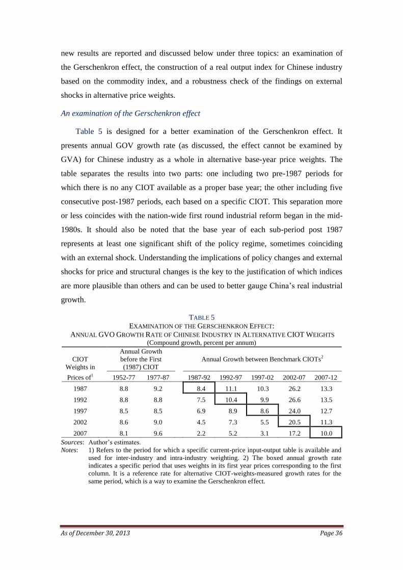
As of December 30, 2013 Page 36
new results are reported and discussed below under three topics: an examination of
the Gerschenkron effect, the construction of a real output index for Chinese industry
based on the commodity index, and a robustness check of the findings on external
shocks in alternative price weights.
An examination of the Gerschenkron effect
Table 5 is designed for a better examination of the Gerschenkron effect. It
presents annual GOV growth rate (as discussed, the effect cannot be examined by
GVA) for Chinese industry as a whole in alternative base-year price weights. The
table separates the results into two parts: one including two pre-1987 periods for
which there is no any CIOT available as a proper base year; the other including five
consecutive post-1987 periods, each based on a specific CIOT. This separation more
or less coincides with the nation-wide first round industrial reform began in the mid-
1980s. It should also be noted that the base year of each sub-period post 1987
represents at least one significant shift of the policy regime, sometimes coinciding
with an external shock. Understanding the implications of policy changes and external
shocks for price and structural changes is the key to the justification of which indices
are more plausible than others and can be used to better gauge China’s real industrial
growth.
TABLE 5
EXAMINATION OF THE GERSCHENKRON EFFECT:
ANNUAL GVO GROWTH RATE OF CHINESE INDUSTRY IN ALTERNATIVE CIOT WEIGHTS (Compound growth, percent per annum)
CIOT
Weights in
Annual Growth
before the First
(1987) CIOT
Annual Growth between Benchmark CIOTs2
Prices of1 1952-77 1977-87
1987-92 1992-97 1997-02 2002-07 2007-12
1987 8.8 9.2
8.4 11.1 10.3 26.2 13.3
1992 8.8 8.8
7.5 10.4 9.9 26.6 13.5
1997 8.5 8.5
6.9 8.9 8.6 24.0 12.7
2002 8.6 9.0
4.5 7.3 5.5 20.5 11.3
2007 8.1 9.6
2.2 5.2 3.1 17.2 10.0
Sources: Author’s estimates.
Notes: 1) Refers to the period for which a specific current-price input-output table is available and
used for inter-industry and intra-industry weighting. 2) The boxed annual growth rate
indicates a specific period that uses weights in its first year prices corresponding to the first
column. It is a reference rate for alternative CIOT-weights-measured growth rates for the
same period, which is a way to examine the Gerschenkron effect.

As of December 30, 2013 Page 37
Specifically, it’s necessary to be aware that, in 1987-88 the government decided
to slow down the pace of price and wage reforms in the wake of unprecedented price
hike since the reform; in 1992 Deng called for bolder reforms that led to the official
adoption of the “socialist market economy” in 1993; in 1997-98, taking stock of the
earlier successful price reforms and a substantial improvement in the supply side of
the economy, the government kicked off more radical ownership reforms; but
meanwhile China was hit by the Asian Financial Crisis that started a five-year long
deflation period; the year of 2002 marked the beginning of China’s post-WTO period
(China was granted WTO membership towards the end of 2011) in which China
emerged as the “world factory”; and the last benchmark 2007 represented China’s
post-WTO performance in the eve of the global financial and economic crisis that
resulted in an unprecedented fiscal spending to save the economy from a significant
global recession.
The expected Gerschenkron effect is clearly evident for the post-1987 period as
shown in Table 5. To help read the results, the boxed annual growth rate indicates a
specific period whose base year is corresponding to the same base-year CIOT weights
shown in the first column. This also helps the examination of estimates in alternative
weights of the same sub-period (presented in columns). The estimated annual growth
rate using more recent base-year price weights is slower than those using any earlier
base-year price weights with the exception of the period 2002-07 and 2007-12 using
the 1987 price weights. The estimates using earlier base-year price weights are more
biased upwards than those using later base-year price weights – this is just as expected.
However, for any of the sub-periods before a specific base-year, the estimates may
contain some downward bias if consumers are rational (and the substitution bias is
held for both before and after the base year). This is also true in our findings for the
post-1987 period. Taking the period 1992-97 as an example, the estimated annual
growth rate is 10.4 percent if using the 1992 price weights, but will be 8.9 and 7.3
percent if shifting to the 1997 and 2002 price weights, respectively.
It shows that for the period 1978-87 and the pre-reform periods, however, the
results are not sensitive to changes of the base-year price weights. This is also
expected for the planning period because of restrict price controls by the planning
authorities. The reform-led as well as market-driven corrections to the previous price
distortions were still limited in the early stage of the reform as represented by the
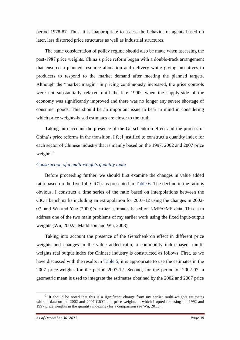
As of December 30, 2013 Page 38
period 1978-87. Thus, it is inappropriate to assess the behavior of agents based on
later, less distorted price structures as well as industrial structures.
The same consideration of policy regime should also be made when assessing the
post-1987 price weights. China’s price reform began with a double-track arrangement
that ensured a planned resource allocation and delivery while giving incentives to
producers to respond to the market demand after meeting the planned targets.
Although the “market margin” in pricing continuously increased, the price controls
were not substantially relaxed until the late 1990s when the supply-side of the
economy was significantly improved and there was no longer any severe shortage of
consumer goods. This should be an important issue to bear in mind in considering
which price weights-based estimates are closer to the truth.
Taking into account the presence of the Gerschenkron effect and the process of
China’s price reforms in the transition, I feel justified to construct a quantity index for
each sector of Chinese industry that is mainly based on the 1997, 2002 and 2007 price
weights.21
Construction of a multi-weights quantity index
Before proceeding further, we should first examine the changes in value added
ratio based on the five full CIOTs as presented in Table 6. The decline in the ratio is
obvious. I construct a time series of the ratio based on interpolations between the
CIOT benchmarks including an extrapolation for 2007-12 using the changes in 2002-
07, and Wu and Yue (2000)’s earlier estimates based on NMP/GMP data. This is to
address one of the two main problems of my earlier work using the fixed input-output
weights (Wu, 2002a; Maddison and Wu, 2008).
Taking into account the presence of the Gerschenkron effect in different price
weights and changes in the value added ratio, a commodity index-based, multi-
weights real output index for Chinese industry is constructed as follows. First, as we
have discussed with the results in Table 5, it is appropriate to use the estimates in the
2007 price-weights for the period 2007-12. Second, for the period of 2002-07, a
geometric mean is used to integrate the estimates obtained by the 2002 and 2007 price
21
It should be noted that this is a significant change from my earlier multi-weights estimates
without data on the 2002 and 2007 CIOT and price weights in which I opted for using the 1992 and
1997 price weights in the quantity indexing (for a comparison see Wu, 2011).

As of December 30, 2013 Page 39
weights. This is to moderate, if not completely cancel, the upward bias of the
estimates with the 2002 price weights and the downward bias of the estimates with the
2007 price weights for the same period. Third, for the same reason, for the period
1997-2002 a geometric mean is also used to integrate the estimates using the 1997 and
2002 price weights.
TABLE 6
RATIO OF GROSS VALUE ADDED TO GROSS VALUE OF OUTPUT IN CHINESE INDUSTRY (GVO=1)
Sector 1980 1987 1992 1997 2002 2007
Energy 0.620 0.563 0.440 0.436 0.449 0.317
Primary inputs 0.363 0.326 0.280 0.295 0.285 0.222
Semi-Finished &
Finished 0.300 0.281 0.244 0.265 0.248 0.197
Total industry 0.383 0.339 0.284 0.301 0.299 0.233
Sources: Calculated based gross value of output data from China Input-Output Table for 1987,
1992, 1997, 2002 and 2007 (DNEB and ONIOS, 1991; DNEA, 1996, 1999, 2005 and
2009).
Note: Figures for 1980 are based on the MPS accounts, estimated by Wu and Yue (2000, p. 97).
Finally, for the period prior to 1997, following the above discussion of the price
reform, it is more appropriate to directly use the estimates in the 1997 price weights
than those in the 1987 and 1992 price weights or any type of integration of these
weights. These annual growth rates are used to derive a 1990-based real output index
for Chinese industry. The results on period-wise growth rates are summarized in
Table 7, whereas the full results in value added in 1990 prices are reported in Table F-
6.
TABLE 7
ANNUAL GROWTH OF ESTIMATED GROSS VALUE ADDED FOR CHINESE INDUSTRY (Compound growth, percent per annum)
Planning Reform
Phases of Reform Period
Sector 1952-77 1977-12
1977-84 1984-91 1991-01 2001-07 2007-12
Energy 13.7 3.8
4.8 1.8 5.5 5.0 0.4
Primary inputs 8.4 6.6
6.7 4.6 6.0 12.2 3.8
Semi-Finished
& Finished 8.6 9.4
9.0 5.3 9.4 17.2 7.1
Total industry 9.1 7.1
7.2 3.5 6.9 13.4 5.5
Total industry
(NBS) 11.3 11.5 9.9 11.2 13.3 12.3 9.8
Sources: Author’s estimates using multi-weights. The NBS estimates are from the national accounts
data of China Statistical Yearbooks.
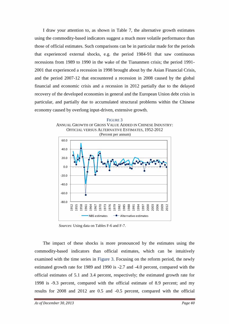
As of December 30, 2013 Page 40
I draw your attention to, as shown in Table 7, the alternative growth estimates
using the commodity-based indicators suggest a much more volatile performance than
those of official estimates. Such comparisons can be in particular made for the periods
that experienced external shocks, e.g. the period 1984-91 that saw continuous
recessions from 1989 to 1990 in the wake of the Tiananmen crisis; the period 1991-
2001 that experienced a recession in 1998 brought about by the Asian Financial Crisis,
and the period 2007-12 that encountered a recession in 2008 caused by the global
financial and economic crisis and a recession in 2012 partially due to the delayed
recovery of the developed economies in general and the European Union debt crisis in
particular, and partially due to accumulated structural problems within the Chinese
economy caused by overlong input-driven, extensive growth.
FIGURE 3
ANNUAL GROWTH OF GROSS VALUE ADDED IN CHINESE INDUSTRY:
OFFICIAL VERSUS ALTERNATIVE ESTIMATES, 1952-2012 (Percent per annum)
Sources: Using data on Tables F-6 and F-7.
The impact of these shocks is more pronounced by the estimates using the
commodity-based indicators than official estimates, which can be intuitively
examined with the time series in Figure 3. Focusing on the reform period, the newly
estimated growth rate for 1989 and 1990 is -2.7 and -4.0 percent, compared with the
official estimates of 5.1 and 3.4 percent, respectively; the estimated growth rate for
1998 is -9.3 percent, compared with the official estimate of 8.9 percent; and my
results for 2008 and 2012 are 0.5 and -0.5 percent, compared with the official
-80.0
-60.0
-40.0
-20.0
0.0
20.0
40.0
60.0
19
52
19
55
19
58
19
61
19
64
19
67
19
70
19
73
19
76
19
79
19
82
19
85
19
88
19
91
19
94
19
97
20
00
20
03
20
06
20
09
20
12
NBS estimates Alternative estimates

As of December 30, 2013 Page 41
estimates of 9.9 and 8.0 percent, respectively. These indeed suggest that whenever
there is an external shock to the Chinese economy, no matter economic or political,
domestic or foreign, the commodity index-based real output measure demonstrates a
much worse performance than what the official statistics tells us. More importantly,
the discrepancy has substantially increased since the reform.
What I would like to emphasize here isn’t, however, that this finding lends strong
support to the institutional argument of the upward-bias hypothesis, which introduces
more or less systematic errors to the growth statistics when the general institutional
conditions do not change. Instead, I would like to argue that it lends important support
to the political economy hypothesis of official statistics that state agencies, statistical
or the like of other ministries, may impose ad hoc adjustments when the economy was
badly hit by an external shock (Wu, 2010). If this is true, there must be a subsequent
counter modification subsequently to “correct” the effect of the ad hoc adjustment to
ensure that the impact of the latter will not screw up the published historical index.
And this modification has to be done professionally. It is no wonder why there appear
to be some smoothing procedures in official estimates, which seem to have moderated
the volatilities picked up by the commodity indicators particularly since 1995. With a
sound extension, the new findings have confirmed the conjecture by Maddison and
Wu (2008) that official estimates tend to smooth out high volatility.
A robustness check of the findings on external shocks
Table 8 is designed to examine if the findings are robust by taking into account
the degrees of price distortions inherited in the different weights. It is quite clear that,
after going through the results using all five price weights, only the 1989-90
Tiananmen Crisis appears to be very sensitive when shifting from the earlier to the
later price weights. The only difference of this shock from others is that it is political
rather than economic directly linked to changes in demand and supply situations,
although it is also external to the operation of the economy but not related to changes
in the international economy.
Not only considering the process of the price reform as discussed above, but also
taking into account the timing of the most recent shocks since the Asian Financial
Crisis, it is justified to focus on the results using the later three price weights, i.e. 1997,

As of December 30, 2013 Page 42
2002 and 2007, especially the last two price weights that are considered more market
based or less distorted, hence more appropriate to address the current situation.
Table 8 shows that shifting between these three price weights indeed does not
significantly change the results regarding for the three recessions, i.e. 1998, 2008 and
2012.22
This not only justifies my approach to the construction of the final real output
index, but also provides strong support to my choice of the indices in different price
weights for different periods (see Table 5 and the discussion).
TABLE 8
ESTIMATED EXTERNAL SHOCKS TO CHINESE INDUSTRY USING
ALTERNATIVE CIOT PRICE WEIGHTS (Percent change over the previous/pre-shock year)
CIOT
Weights in
Prices of
Energy
Primary
inputs
Semi-
finished &
finished
Total
Industry
1989-90 Tiananmen Crisis1
1987 -5.2 -3.1 -8.9 -2.0
1992 -5.1 -3.1 -11.5 -4.1
1997 -5.3 -3.7 -13.4 -6.8
2002 -6.0 -12.6 -15.1 -10.2
2007 -7.0 -18.9 -14.8 -13.7
1998 Asian Financial Crisis2
1987 1.5 -3.3 -14.9 -7.5
1992 1.1 -4.1 -14.2 -7.8
1997 1.6 -5.6 -13.8 -8.0
2002 1.3 -11.7 -16.3 -10.8
2007 1.2 -13.6 -18.3 -10.6
2008 Global Financial & Economic Crisis
1987 -1.2 0.2 -0.3 -0.3
1992 -1.4 0.4 -0.8 -0.3
1997 -1.2 0.4 -0.4 -0.8
2002 -1.5 1.2 1.7 0.2
2007 -1.5 0.5 2.7 0.5
2012 GFC Aftermath & EU Debt Crisis
1987 -1.0 0.2 -2.1 -1.5
1992 -0.7 0.3 -0.6 0.4
1997 -1.4 0.0 -0.5 -0.2
2002 -1.5 -0.4 -0.9 -0.3
2007 -1.4 0.0 -1.3 -0.5
Sources: Author’s estimates.
Notes: 1) The figures are shown as percent change in 1990 over 1988 as
the commodity indicators pick up two consecutive declines in
1989 and 1990. 2) AFC began in 1997 but China was mainly hit
in 1998. This part refers to percent changes in 1998 over 1997.
22
Table 8 is not designed to directly work out the final results used in Figure 3. To arrive at the
final estimates, one needs to refer to the earlier discussion. Basically, the estimated growth rate for
1989 and 1990 is based on the 1997 prices weights, for 1998 based on the geometric mean of the
growth rates estimated by the 1997 and 2002 price weights, and for 2008 and 2012 is based on the 2007
price weights.

As of December 30, 2013 Page 43
A reply to the quality problem critique
One of the criticisms to my commodity index-based real output index for Chinese
industry is that it underestimates the effect of quality change. This is to say that the
quality change is implicitly counted as a price effect in the exercise and hence being
removed in the construction of the quantity index (Holz, 2006a; Rawski, 2008).
It is certainly not easy to maintain product homogeneity in this kind of exercise.
However, there are many products used that are homogenous in nature, e.g. coal, iron
ore, salt, basic metals and basic chemicals. More heterogeneous products such like
pressed steel products are measured by types with information on price and quantity
rather than in aggregate tonnage, similarly for many producer goods from chemical
fertilizers, refined oil products to semi-conductors.23
Despite these efforts, some
underestimation of the quality change may still exist. The question is, however, the
seriousness of the quality problem in the constructed quantity index.
FIGURE 4
DOES WHAT IS MISSED SUGGEST A REASONABLE TREND OF QUALITY CHANGE? (Percentage-point difference by subtracting alternative estimates from NBS estimates)
Sources: Figure 3.
23
Instead of constructing simple quantity index by the units of all (mixed) semi-conductors
produced as reported by DIS, I worked on six major types of semi-conductors with their ex-factory
prices and quantities and went through two levels of aggregation to obtain an average price for the
single CIES item “semi-conductor” for each benchmark year, i.e. 6.13 yuan for 1987, 2.61 yuan for
1992, 1.88 yuan for 1997, 1.33 for 2002 and 1.01 for 2007, respectively. Semi-conductor may be an
atypical case as it has experienced tremendous quality increase and significant price decline. Yet, my
procedures show that quality change in this case is not completely uncounted.
-20.0
-15.0
-10.0
-5.0
0.0
5.0
10.0
15.0
20.0
19
53
19
56
19
59
19
62
19
65
19
68
19
71
19
74
19
77
19
80
19
83
19
86
19
89
19
92
19
95
19
98
20
01
20
04
20
07
20
10

As of December 30, 2013 Page 44
Notes: Shocks identified in Figure 3 are excluded in order to obtain
more reliable estimates for a “quality trend”.
Fortunately, the way in which we apply different price weights to the exact same
set of commodity data for the same period provides us an advantage for examining the
quality problem in the commodity index-based real output index. The official index
can be used as a “benchmark”. We can assume that the percentage-point differences
by subtracting the alternative estimates from official estimates contain mainly the
missing quality, thus the change of the so-derived differences over time can be taken
as an indicator of the trend of quality change in Chinese industry. Note that to obtain a
reliable measure, the external shocks identified in Figure 3 have to be removed from
the calculation.
The results are presented in Figure 4. It is reasonable to expect that the missing
quality should be steadily rising over time especially since the economic reform. To
facilitate the examination I add a polynomial trend to filter out the noise. If the
critique were correct and the gap indeed mainly contains the missing quality change,
China’s industrial development appears to be first undergoing a continuous quality
deterioration for about 20 years until the early 1970s, which is implausible even if the
inefficiency of the central planning period is considered, then followed by a slow
quality improvement till the early 1990s before China adopted the “socialist market
economy” system, and a further rapid decline along with deepening industrial reforms
and China’s participation in WTO till the present time, which does not look plausible
at all.
Impact of the alternative estimates
It is useful to examine the impact of my alternative GDP estimates for Chinese
industry upon the officially estimated total GDP growth. This is presented in Table 9.
It shows the effect of my estimates-implied growth on the official GDP growth for the
total economy, holding the official GDP estimates for the rest of economy unchanged.
It shows that the impact of my adjustment is 0.45 percentage points on the growth
of the planning period but -1.77 percentage points on the growth of the reform period,
other things being equal. Again, at the aggregate level, my results have substantially
adjusted downwards the growth performance of the period when there was an external
shock (the time of 1989/90 in the period 1984-91 and 1998 in 1991-2001). For the
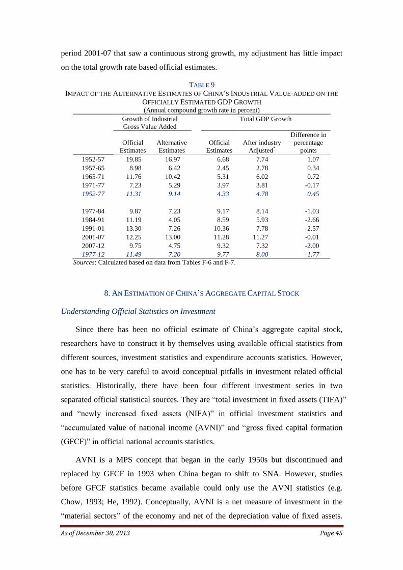
As of December 30, 2013 Page 45
period 2001-07 that saw a continuous strong growth, my adjustment has little impact
on the total growth rate based official estimates.
TABLE 9
IMPACT OF THE ALTERNATIVE ESTIMATES OF CHINA’S INDUSTRIAL VALUE-ADDED ON THE
OFFICIALLY ESTIMATED GDP GROWTH (Annual compound growth rate in percent)
Growth of Industrial
Gross Value Added
Total GDP Growth
Official
Estimates
Alternative
Estimates
Official
Estimates
After industry
Adjusted*
Difference in
percentage
points
1952-57 19.85 16.97 6.68 7.74 1.07
1957-65 8.98 6.42 2.45 2.78 0.34
1965-71 11.76 10.42 5.31 6.02 0.72
1971-77 7.23 5.29 3.97 3.81 -0.17
1952-77 11.31 9.14 4.33 4.78 0.45
1977-84 9.87 7.23 9.17 8.14 -1.03
1984-91 11.19 4.05 8.59 5.93 -2.66
1991-01 13.30 7.26 10.36 7.78 -2.57
2001-07 12.25 13.00 11.28 11.27 -0.01
2007-12 9.75 4.75 9.32 7.32 -2.00
1977-12 11.49 7.20 9.77 8.00 -1.77
Sources: Calculated based on data from Tables F-6 and F-7.
8. AN ESTIMATION OF CHINA’S AGGREGATE CAPITAL STOCK
Understanding Official Statistics on Investment
Since there has been no official estimate of China’s aggregate capital stock,
researchers have to construct it by themselves using available official statistics from
different sources, investment statistics and expenditure accounts statistics. However,
one has to be very careful to avoid conceptual pitfalls in investment related official
statistics. Historically, there have been four different investment series in two
separated official statistical sources. They are “total investment in fixed assets (TIFA)”
and “newly increased fixed assets (NIFA)” in official investment statistics and
“accumulated value of national income (AVNI)” and “gross fixed capital formation
(GFCF)” in official national accounts statistics.
AVNI is a MPS concept that began in the early 1950s but discontinued and
replaced by GFCF in 1993 when China began to shift to SNA. However, studies
before GFCF statistics became available could only use the AVNI statistics (e.g.
Chow, 1993; He, 1992). Conceptually, AVNI is a net measure of investment in the
“material sectors” of the economy and net of the depreciation value of fixed assets.
As of December 30, 2013 Page 46
But, on the other hand, it is an incomplete and “dirty” indicator because it not only
excludes investment in all “non-material activities” but also mixes up fixed asset
investment, circulation funds and inventory. Therefore, it has no theoretical
underpinning if simply adding up the annual AVNI flows to construct a capital stock
series for the economy. Under the Chinese SNA, the Department of National
Economic Accounts (DNEA) of NBS has adjusted the historical AVNI series to
construct a series of GFCF (DNEA, 1997). The GFCF series has since been revised
twice (DNEA, 2004 and 2007).
TIFA also has a long history dating back to the beginning of the 1950s. It was
designed to measure investment projects above certain size in value terms at current
prices, available with breakdowns in investment types which are the only information
for gauging asset types,24
ownership types, by sector/industry and by source of
funding. The data collection for TIFA is conducted through the investment monitoring
authorities at different levels of administration and published by DFAIS (Department
of Fixed Asset Investment Statistics) of NBS.
Due to insufficient coverage and conceptual problems, TIFA should not be
directly used as the investment variable in the perpetual inventory method equation as
done in many existing studies (Ho and Jorgenson, 2001; Hu and Khan, 1997; Huang
et al., 2002; Li et al., 1992; Ren and Sun, 2007; Young, 2003). Firstly, TIFA excludes
all fixed asset investment projects that is smaller than half million yuan and all
intangible assets. More problematically, it includes the transaction of existing assets
typically land that rocketed in the last decade,25
creating serious doubling counting
problem. However, the coverage problem including land transaction-related double
24
TIFA consists of three categories that distinguish fixed asset investment by nature, namely,
“construction and installation”, “purchase of equipment”, and “other expenses” that are largely
consumables to facilitate the above two activities (DFAIS, 1997, pp.444-445).
25 In China, land belongs to the state or semi-state organizations (“collectives”) as in the case of
farm land. There is no ownership transfer-based land transaction, but only the trade of “land use rights”.
However, the government (both central and local) controls the primary release of the land use rights
according to land size, location and market situation (unit price and timing). There have been
increasing criticisms on the land-related government revenue and land-financed local public spending
that has been considered largely responsible for China’s property bubbles ricking the financial system
(Zhu, 2011).

As of December 30, 2013 Page 47
counting has largely been tackled in the construction of the national accounts. In this
sense, GFCF is more qualified as an investment indicator than TIFA.26
Besides, TIFA has a serious conceptual problem because it blurs the line between
fixed capital formation and inventory. It is by official definition a measure of the
workload in the construction and purchase of fixed assets in money terms (NBS, 2001,
p.220; DFAIS, 1997, p.444). As correctly noted in Chow (1993, p.816), the work
performed and recorded in TIFA may not eventually produce results that meet
production standards for fixed assets in the current period. In fact, some of the work
(investment projects) may take many years to become qualified for productive assets
and some may never meet the standards, hence be completely wasted, which is a
typical phenomenon observed in all centrally planned economies.
The nature of the problem shows a significant conceptual and practical difference
between China’s national accounts and SNA. The SNA principle governing the time
of recording and valuating fixed capital formation is “when the ownership of the fixed
assets is transferred to the institutional unit that intends to use them in production”
(CEC et al, 1993, p.223). Xu (1999, pp.62-63) notes that in SNA a plant construction
is counted as inventory if it cannot be sold to a buyer (investor) or cannot be used in
production but it is included as investment in fixed assets in TIFA. The problem is
aggravated in the case of a large project that needs several stages (years) to complete
in which the investment “workload” is counted at each stage but the project cannot be
used for production before all stages are completed.
By concept NIFA is designed to measure the completed fixed assets projects in
value terms that are transferred to investors or users in the current period. As shown in
the conceptualization for NIFA in Wu (2008), it is the current year completed and
recorded result of TIFA initiated in the current and in all the previous years. NIFA
appears to be a better indicator than TIFA but it is by no means flawless. Firstly, since
NIFA is originated in TIFA, it has been affected by the same coverage and double
counting problems as in TIFA. There is nosystem that checks and removes the
double-counted land value when a project is completed. Secondly, as required by the
statistical authority, “to timely show the achievement in fixed asset investment,
26
As observed at localities, TIFA statistics are manipulated by local officials in order to meet
growth target: some non-investment spending are reported as fixed asset investment; some previously
completed projects are repeatedly reported to exaggerate growth performance; and some planned future
projects are reported as actual investment.

As of December 30, 2013 Page 48
completed projects should be generally counted as currently in operation even if they
are not yet quality-verified and passed” (DFAIS, 1997, p.448). Thus, even if NIFA
does not exaggerate the actual fixed capital formation it will still have a different
growth pattern from that of the true capital stock in the economy. Lastly, NIFA has
inherited a complicated price problem from TIFA. It is never clear whether the
valuation in NIFA is at current prices or the prices recorded in TIFA in the years of
investment. However, since the workload approach is used in the valuation of TIFA,
one may reasonably believe that the completed projects recorded in NIFA are also
valued in multiple historical prices.
FIGURE 5
COULD THE RELATIONSHIP BETWEEN TIFA, NIFA AND GFCF BE GAUGED? (TIFA=1; GFCF=1)
Sources: Author’s reconstruction based on data from NBS (2012, Tables 2-17,
5-2 and 5-20, and other issues) and DNEA (2004 and 2007).
Based on all these considerations, studies that relied on the official so-called
“transfer rate”27
(DFAIS, 1997, p.174), which is measured as NIFA divided by TIFA,
to estimate the “real” GFCF have inevitably included serious flaws (Wang and Fan,
2000; Holz, 2006b; Wang and Szirmai, 2012). Although NIFA and TIFA can be
connected in theory, they are conceptually incompatible (Wu, 2008b). There is no
regularity that makes NIFA predictable by TIFA because the average time used for a
given amount of investment in fixed assets not only depends on the size and type of
27
The official English translation of this ratio is recently changed to “Rate of fixed assets projects
completed and put in use” (see for example NBS, 2009, p.206).
0.0
0.2
0.4
0.6
0.8
1.0
1.2
1.4
1.6
1.8
19
80
19
81
19
82
19
83
19
84
19
85
19
86
19
87
19
88
19
89
19
90
19
91
19
92
19
93
19
94
19
95
19
96
19
97
19
98
19
99
20
00
20
01
20
02
20
03
20
04
20
05
20
06
20
07
20
08
20
09
20
10
20
11
20
12
NIFA/TIFA NIFA/GFCF TIFA/GFCF

As of December 30, 2013 Page 49
investment but also depends on the behavior of investors that is affected by ownership
form, governing policy and institutional environment.
An Adjustment to GFCF
Based on the above discussion, GFCF is relatively more appropriate for the
investment variable required in our estimation of net capital stock for the Chinese
economy. GFCF is now available as part of the national expenditure accounts starting
in 1952 together with inventory, private and government consumption and net export
(DNEA, 2007). However, it is still not clear how NBS constructs GFCF from TIFA
and NIFA. One cannot simply presume that the official GFCF series is problem free.
In the present work, I do not directly use the official GFCF, here denoted as
GFCF(A) in Table 10. Instead, I first remove the investment in residential housing (as
an unproductive asset) to obtain a new series of GFCF(B), and then construct a new
series of GFCF(C) by applying the share of the official GFCF in the gross domestic
expenditure accounts to my alternative GDP estimates (Table F-6). This is to ensure a
conceptual consistency with my GDP adjustment. As Table 10 shows, in nominal
terms, the movements of GFCF are closer to those of NIFA rather than TIFA. The
housing adjustment has a downward effect of 0.2 percentage points for the planning
period and 0.7 percentage points for the reform period. I leave the discussion of
changes of investment prices in different measures and the further adjustment to
derive the series of GFCF(C) after the sub-section on deflator.

As of December 30, 2013 Page 50
TABLE 10
OFFICIAL AND ALTERNATIVE ESTIMATES OF ANNUAL INVESTMENT GROWTH, AND THE SHARE INVESTMENT IN CHINA’S GDP (Annual compound growth in percent in nominal or 1990 prices, unless specified)
GFCF in Nominal Prices
Price Change of GFCF
GFCF(B) in 1990 Prices
GFCF(C)5 in 1990 Prices
TIFA1 NIFA
1 GFCF(A)
2 GFCF(B)
2
Official
IPI3
Alternative
IPI4
Official
IPI
Alternative
IPI
Alternative
IPI
Share6
(GDP=1)
1952-57 28.3 13.1 18.3 17.7
-2.1 -2.3
20.3 20.5
19.9 0.09
1957-65 4.6 5.9 8.2 8.2
1.6 1.6
6.5 6.4
7.3 0.16
1965-71 11.5 10.9 9.5 9.0
-1.1 -1.1
10.1 10.2
9.9 0.17
1971-77 4.7 4.5 7.1 7.1
0.8 -2.3
6.3 9.7
9.1 0.23
1952-77 10.7 7.9 10.2 10.0
0.0 -0.8
9.9 10.8
10.8 0.16
1977-84 16.7 13.4 13.0 12.1
2.7 3.1
9.2 8.8
7.4 0.25
1984-91 17.3 17.6 16.0 16.8
8.0 7.5
8.2 8.7
5.2 0.27
1991-01 20.9 19.7 20.1 19.3
5.9 2.3
12.7 16.7
13.3 0.41
2001-07 24.3 19.8 18.4 15.0
2.7 2.0
11.9 12.7
11.4 0.52
2007-12 22.2 21.8 18.5 19.5
3.4 3.2
15.6 15.8
12.9 0.62
1977-12 20.1 18.3 17.3 16.6
4.8 3.5
11.3 12.7
10.1 0.40
Sources: Author’s estimates. For the basic data, see Figure 5.
Notes: 1) TIFA and NIFA are as defined in text. 2) GFCF(A) includes residential housing and GFCF(B) removes residential housing. 3) The official
investment price index (IPI) is the expenditure accounts implicit deflator. 4) The alternative IPI is constructed based on PPI of investment goods
industries, see text for details. 5) GFCF(C) is alternative GDP-adjusted GFCF(B). 6) The share of GFCF is estimated as GFCF(C)/alternative GDP
in 1990 prices.

As of December 30, 2013 Page 51
The Initial Capital Stock
Despite many efforts which have been made in estimating China’s aggregate
capital stock,28
the estimation of its initial (post-war) stock has been left ambiguous.
Existing studies have made or adopted very different estimates for the initial capital
stock (usually referring to 1952) ranging greatly from less than 50 to over 250 billion
yuan in 1952 prices which imply a capital-output ratio (K/Y) ranging from below 0.45
to a level as high as over 2 if based on the official GDP for 1952. Some may argue
that the initial stock in the early 1950s does not really matter if the main interest is in
the reform period and in growth accounting (Young, 2003, p.1253). But it is however
important if we are interested in examining changes in capital-labor ratio, capital-
output ratio and the trend of return on capital in the Chinese economy in the long run.
Few of the studies have discussed how their estimates are made. Maddison
(1998a, pp.64-65) relied on a hypothetical capital-output ratio of 0.9 for 1952 that was
empirically justified by the lower bound of the international standard and pre-war
estimates by Yeh (1968 and 1979). I will use this as a reasonable starting point in the
following discussion. My research on the initial capital stock follows two lines: one is
theoretical which assumes a steady state situation for China in the early 1950s using
an approach as explained in King and Levine (1994), and the other one is empirical
which uses the data of China’s first asset census in 1951 (SETC, 2000, Vol. 1).
The estimation of the initial capital stock follows the steady-state method as in
King and Levine (1994). Let us assume that physical capital and the real output grow
at the same rate *, that is,
(8.1) t
t
t
tt
Y
dY
K
dK*
where tK is the capital stock and tY is real GDP at time t. Since ttt KIdK then
t
t
t
t
K
I
K
dK where tI is gross investment and δ is the depreciation rate of physical
28
For studies in English see, e.g. Chow (1993), Chow and Li (2002), Field (1980), Holz (2006b),
Hu and Khan (1997), Maddison (1998a), Wang and Szirmai (2012), Wang and Yao (2002), and Young
(2003). For studies in Chinese see e.g. Bai et al (2007), He (1992), He et al (2003), Ren and Liu (1997),
Tang (1999), Wang and Fan (2000), and Zhang and Zhang (2003).

As of December 30, 2013 Page 52
capital. Letting i be the investment rate, i.e. t
tt
Y
Ii , thus
t
tt
t
tt
K
Yi
K
dK* , then the
steady-state capital-output ratio is derived as follows:
(8.2) *
**
t
tt
i
that is,
*
*
t
tt
IK
.
To estimate physical capital stock at time t by the standard perpetual inventory
method (PIM), the following equation is applied:
(8.3) ttt KIK )1(1
Then, based on (8.3) we can generate a function of initial capital stock and investment
flows as follows:
(8.4) 0
1
0
)1()1( KIK tit
t
i
it
where 0*
0 YK t
To solve for 0K of Equation 8.4, we need data on investment flows, an average
GDP growth rate and a depreciation rate for the initial period. The national accounts
GFCF in 1952 can be used for 0I , official and my alternative measures of the average
GDP growth for the period 1952-56 are used for g , and 0 is assumed to be 2
percent based on the information from the 1951 national asset census (explained
below).
Directly using the unadjusted official GFCF, GDP and the expenditure accounts
implicit GFCF deflators, plus the 2-percent depreciation rate as revealed by the 1951
asset census, I obtain an initial capital stock of 166.7 billion in 1990 yuan for the
midpoint time of 1952-57 (e.g. 1955) based on which the average GDP growth rate is
calculated. However, if using my alternative estimates of GFCF, GDP and GFCF
deflator, and choosing a 5-percent depreciation rate, the results would be 208.3 billion
1990 yuan. And if I use Maddison’s assumption of a K/Y ratio of 0.9, I can obtain an
estimate of 286.5 billion 1990 yuan for 1952 using my new estimate of GDP.
I evaluate the above estimates by examining seldom used information from the
aforementioned 1951 national asset census that verified and evaluated China’s stock
of fixed assets, only available for publication in 2000 as a collection of archived

As of December 30, 2013 Page 53
planning documents and papers by SETC (2000, Vol. 1, pp.1543-4). It shows that by
the end of 1951, the total market replacement value of fixed assets was 128.4 billion
in 1952 yuan. Taking off the accumulated depreciation value of 39.2 billion, the net
stock would be 89.2 billion 1952 yuan, equivalent to 169.6 billion 1990 yuan (based
on 1990/1952 investment price ratio 1.901 by the NBS deflator).
However, one should not take this asset census data for granted. Two political
economy factors have to be taken into account when evaluating this census results. On
one hand, the private owners of fixed assets had strong incentives to hide some assets
in a state-run survey because of a high fear of confiscation or nationalization. On the
other hand, the authorities also tended to undervalue private assets in order to reduce
the purchase cost of the assets should the sate decide to buy rather than to confiscate
them.
There is clear evidence in the census data that the fixed asset in the agricultural
sector, dominated by private farmers, is implausibly low – only 0.04 percent of the
total net stock. Land is certainly not included. But that is not our problem, at least for
the current work as land is also not included. However, we can show that this census
result is absolutely implausible only using the information from state-owned farms. In
1952, the land area of state-owned farms, inherited from the old government after the
1949 revolution, accounted for 3.5 percent of the national arable areas. Since state
farms were operated with more machinery, draught animals and productive structures
than private and household farms, it is reasonable to assume that the fixed assets
owned by the state farms may account for at least 10 percent of the total assets in
agriculture. Chow (1993) also conjectures that the initial agricultural capital stock
should account for 30 percent of the national total excluding land.
I then make an estimation based on the following (still conservative) assumptions:
10 percent of the fixed assets in industry and services were underestimated and after
an adjustment for the 10 percent underestimation the value of non-agricultural fixed
assets should be accounted for 70 percent of the national total. The residual estimate
from this calculation refers to the fixed assets in agriculture. The so-estimated total
value of fixed assets is 140.1 billion 1952 yuan for 1951, of which agriculture
accounted for 30 percent, industry 8 percent and service 62 percent. After
depreciation and an adjustment to the price change between 1952 and 1990, it would
be 287.2 billion 1990 yuan. Next, based on the real growth of fixed asset investment
As of December 30, 2013 Page 54
between 1951 and 1952, 14.3 percent (CASS and CA, 1998, pp.1138-42), the
comparable value for 1952 is estimated at 328.3 billion 1990 yuan, which is not too
far away from the estimate of 286.5 billion 1990 yuan based on Maddison’s
assumption. This result (328.3 billion 1990 yuan) is used as the initial capital stock for
1952 in my PIM exercise.29
Depreciation Rate
Based on Equation 8.4 two sets of net capital stock series are constructed, each
using the same alternative depreciation rates proposed in this study based on my
earlier work on an industry-level estimation of capital stock (Wu, 2008b).
Following Hulten and Wykoff (1981), I assume that industry-specific
depreciation rate, i=Ri /Ti, where T stands for the service life of an industry and
function-specific asset which is based on official accounting regulations (State
Council, 1985; Ministry of Finance, 1992), and R is the asset’s declining balance rate
based on the empirical findings in Hulten and Wykoff (1981). The estimated
depreciation rates for 39 two-digit level industries are on average ranged from 7 to 8.5
percent for equipment and 2.5 to 3.5 percent for structures over three available time
points, i.e. 1963, 1985 and 1993 (Wu, 2008b). Considering the likelihood of a market-
induced faster depreciation process following the reform, as well as the underlying
faster economic depreciation before the reform, it is reasonable to increase these
estimates to 10 percent for equipment and 4 percent for structures in industry. This is
a basis for us to gauge an average general depreciation rate for the economy as a
whole. In Chinese industry, as evidenced in Wu (2008b) equipment accounts for 70
percent of the fixed assets and structures for 30 percent. This is reversed when
focusing on the asset structure of the national economy based on investment, that is,
approximately 35 percent for equipment and 65 percent for structures excluding
housing, based on official investment statistics. Therefore, an average depreciation
rate for the whole economy is about 6 percent (6.1%=10%*0.35+4%*0.65).
Therefore, the present study sets a depreciation rate of 6 percent (=0.06) as the
baseline with 5 and 7 percent as the lower and upper bound, respectively. These are
29
Based on the same achieve data (CASS and CA, 1998) on the growth of fixed asset investment
over 1949-53, I also obtain an estimate of 256.6 billion for 1949, 267.3 billion for 1950 in 1990 yuan.

As of December 30, 2013 Page 55
alternative depreciation rates for the entire period in question assuming that the
depreciation process in the Chinese economy follows a geometric function.30
An Alternative Investment Deflator
I construct an alternative investment deflator to the official GFCF deflator that is
implicitly given by the expenditure accounts for two reasons. First, the implicit
GFCF-IPI may have overstated the price changes in the period 1995-2004 in which
China experienced an unprecedented long deflation in investment goods, much longer
than that experienced by the general economy in 1998-2002. Second, the implicit
GFCF-IPI is highly likely to be influenced by the rapidly rising prices of land
transactions along with China’s property boom in the 2000s. As Figure 6 shows, since
the mid-1990s, the implicit GFCF-IPI has mainly followed the PPI (producer price
index) of building materials rather than the PPI of equipment industries. However, the
PPI of building materials well reflects the effect of the long deflation in the Chinese
economy but the GFCF-IPI does not. This justifies the use of a PPI weighting both the
PPI of building materials and the PPI of equipment industries.
In the construction of the alternative IPI, I first construct two weighted PPIs: one
PPI is based on the PPIs of construction materials industries, namely, non-metallic
materials and basic and fabricated metals, and the other PPI is based on the PPIs of
machinery and equipment industries including ordinary and special purpose
machinery, transportation equipment, electrical and electronic equipment and office
equipment (Figure 6). I then further weight the two so-constructed PPIs into one IPI,
the alternative IPI as depicted in Figure 6.
Table 10 already includes a comparison of the implicit GFCF IPI with my
alternative IPI. For the planning period, the GFCF IPI shows that there was no change
in investment prices but my deflator suggests a decline by 0.8 percent in investment
prices. For the reform period, however, the alternative IPI also implies a slower
change of investment prices than the official IPI does, i.e. 3.5 compared with 4.8
30
Besides, taking into account an increasing market influences on firms’ depreciation decision
that may have speeded up the depreciation process over time, we can also introduce a multiple-
depreciation process by assuming 5 percent for the pre-reform period, 6 percent for the early reform
period 1978-91, then 7 percent for the period from 1992 onwards up to 2008, and further 8 percent in
the wake of the global financial and economic crisis, allowing a “smooth transition” over five years
around the benchmarks to avoid breaks. This alternative treatment may be justifiable for reflecting
changes of producers’ behavior in response to the shifts of policy regimes that promote market
competition, but it does not satisfy the theory of economic depreciation.

As of December 30, 2013 Page 56
percent per annum. Consequently, using the alternative IPI will raise the growth of
GFCF from 9.9 to 10.8 percent per annum for the planning period and from 11.3 to
12.7 percent for the reform period. It should be noted that other things being equal,
this will raise rather than lower the growth of TFP.
FIGURE 6
WHICH INVESTMENT DEFLATOR IS MORE REASONABLE? (1990=100)
Sources: NBS (2012, Tables 2-17, 9-11, 9-12 and other issues), DNEA (2004 and
2007) and EC (2002).
TABLE 11
ESTIMATED ANNUAL GROWTH OF NET CAPITAL STOCK BY OFFICIAL AND ALTERNATIVE
DEFLATORS AND BY DIFFERENT DEPRECIATION RATES (Annual percentage change)
Net Capital Stock by GFCF(B) and
Official Investment Deflator
Net Capital Stock by GFCF(C) and
Alternative Investment Deflator
=0.05 =0.06 =0.07 =0.05 =0.06 =0.07
1952-57 4.03 3.21 2.39 5.54 4.74 3.95
1957-65 6.34 5.91 5.50 7.44 7.04 6.65
1965-71 5.87 5.75 5.66 6.87 6.77 6.70
1971-77 7.74 7.77 7.82 8.94 8.99 9.06
1952-77 6.09 5.77 5.46 7.28 6.97 6.69
1977-84 7.23 7.22 7.22 7.92 7.88 7.85
1984-91 9.19 9.27 9.35 7.69 7.65 7.61
1991-01 11.21 11.31 11.41 10.82 10.95 11.08
2001-07 11.19 11.22 11.25 10.92 10.95 10.98
2007-12 13.06 13.16 13.25 11.53 11.57 11.61
1977-12 10.25 10.32 10.38 9.72 9.75 9.79
Source: Calculated based on data in Table F-8.
Table 11 shows the growth rate of net capital stocks estimated by different IPIs
and at different depreciation rates, which demonstrates different dynamics in different
0
50
100
150
200
250
300
19
52
19
56
19
60
19
64
19
68
19
72
19
76
19
80
19
84
19
88
19
92
19
96
20
00
20
04
20
08
20
12
1990 = 100
NBS GFCF-IPI Alternative IPI
Bdng mat. PPI Machinery PPI
70
80
90
100
110
120
130
140
19
52
19
56
19
60
19
64
19
68
19
72
19
76
19
80
19
84
19
88
19
92
19
96
20
00
20
04
20
08
20
12
Last year = 100
NBS GFCF-IPI Alternative IPI

As of December 30, 2013 Page 57
periods from that of GFCF in Table 10. Examining our baseline estimates with =0.06,
compared with the official deflator-based results my alternative deflator-based results
provide a faster growth of net capital stock for the planning period but a slower
growth for the reform period.
TABLE 12
INVESTMENT-CAPITAL RATIO, CAPITAL-OUTPUT RATIO AND “RETURNS ON CAPITAL” (Annual average)
MPK (“Returns on Capital”)
I/K K/Y Y/K*.6 Y/K*.4 Y/K*φ
1952-57 0.10 0.99 0.61 0.40 0.42
1957-65 0.12 1.38 0.45 0.30 0.34
1965-71 0.12 1.40 0.43 0.29 0.36
1971-77 0.14 1.69 0.36 0.24 0.32
1952-77 0.12 1.37 0.46 0.31 0.36
1977-84 0.13 1.98 0.30 0.20 0.28
1984-91 0.13 2.15 0.28 0.19 0.25
1991-01 0.15 2.71 0.23 0.15 0.19
2001-07 0.15 3.42 0.18 0.12 0.16
2007-12 0.16 3.95 0.15 0.10 0.15
1977-12 0.14 2.75 0.23 0.16 0.21
Sources: Tables F-6, F-7 and F-8.
Notes: Y refers to my alternative GDP estimates; I is GFCF(C) using the alternative deflator;
K refers to net stock based on δ=.06; the capital share of the national income is given as 0.6
following Chow (1993), 0.4 following Young (2003) and my time-variant estimates (φ)
based on the Chinese input-output tables.
Table 12 presents the annual average of investment-capital ratio (I/K) and capital-
output ratio (K/Y) for both the planning and reform periods. These measures are
based on all my alternatively constructed variables: GDP, GFCF(C) and investment
deflator. While the change of I/K is insignificant over periods, the change of K/Y is
indeed substantial from about 1 in 1952-57 to nearly 4 in 2007-12. Based on the
World Bank data for 2010, using the same approach, we can show that countries at
much higher level of development did not reach this level, e.g. 3.6 for Japan, 3 for
South Korea and Germany, and 2.5 for US. It seems that China is undergoing a
premature transition from labor-intensive to capital-intensive development. This is,
however, not only a sign showing China’s high reliance on investment-driven growth
but more an indicator to inefficient investment. The dynamics of I/K and K/Y and a
comparison between estimates using the different investment deflators are shown in
Figure 7.

As of December 30, 2013 Page 58
This can be further supported by a measure of “returns on capital” as marginal
product of capital (i.e. Y/K adjusted by the capital share in the national income). As
correctly put by Chow (2006), one of important assessments of the estimated capital
stock is the rate of return to capital implied by the capital stock. Table 12 also
provides three sets of estimates for all sub-periods based on different “capital income
shares in national GDP”, i.e. a fixed 60 percent following Chow (1993) and also
Chow and Li (2002), and a fixed 40 percent following Young (2003) and my time-
variant measure based income shares from China’s input-output tables and their
extensions.
FIGURE 7
INVESTMENT-CAPITAL STOCK (I/K) RATIO AND CAPITAL-OUTPUT (K/Y) RATIO BY OFFICIAL
AND ALTERNATIVE INVESTMENT DEFLATORS, 1952-2012
Source: Table 12.
As cited in Chow (2006), for 1954 Chow’s estimated capital stock implies a rate
of return to capital of 0.22 (different from what I have estimated based on Chow’s 60-
percent income share for capital, which is 0.61, an average rate of 1953-55), whereas
Holz (2006b)’s work implies the rate as 0.99. Based on a market economy assumption
for the Chinese economy in the early 1950s, Chow considers that Holz’s result is
implausible. Although there are conceptual problems in Holz’s work, assuming that
the economy in the early 1950s was still a typical market one could also be
questionable based on clear evidence that the state already owned and controlled the
majority of the modern sector of the economy and initiated a radical
“corporatization/socialization” in the farm and service sectors by 1954/55. However,
for that stage of development a somewhat higher rate of return to capital may be
0.00
0.05
0.10
0.15
0.20
0.25
19
52
19
56
19
60
19
64
19
68
19
72
19
76
19
80
19
84
19
88
19
92
19
96
20
00
20
04
20
08
20
12
I/K (Official IPI) I/K (Alternative IPI)
0.00
0.50
1.00
1.50
2.00
2.50
3.00
3.50
4.00
4.50
5.00
19
52
19
56
19
60
19
64
19
68
19
72
19
76
19
80
19
84
19
88
19
92
19
96
20
00
20
04
20
08
20
12
K/Y (Official IPI) K/Y (Alternative IPI)

As of December 30, 2013 Page 59
reasonable though it may not be as high as what Holz’s results imply. For a
comparison, the rate implied by my estimated capital stock is 0.42 and by Wang and
Szirmai’s work is 0.67, both substantially lower than that of Holz.31
FIGURE 8
“RETURNS ON CAPITAL” (MPK) OF THE CHINESE ECONOMY, 1952-2012 A. Using NBS GFCF-IPI B. Using Alternative IPI
Source: Table 12.
Note: MPK(A), MPK(B) and MPK(C) are based on 60 percent, 40 percent and
time-variant input-output table capital share in national income.
For the most recent period 2007-12, based on the input-output table income share,
China’s MPK is only 0.15. Although it is still somewhat higher than the developed
countries (the US is .12, Japan is .08 and Germany and South Korea is .10 for 2010),
which should not be a big surprise, it is obviously too low if comparing with countries
like Brazil (2.7) and India (2.6). The dynamics of alternative estimates of MPK and a
comparison between estimates using the different deflators are presented in Figure 8.
Although the economic history shows that income growth in general is
accompanied by diminishing returns to capital, in some economies this process can be
slowed down or even turned around for some time by productivity advancement.
There are interesting observations in Figure 8 which can be used to assess if my
alternative estimates are reasonable. Let us use the results based on the time-variant
input-output table capital share in national income as our baseline estimates. The
31
All of these estimates conform to the “diminishing return to capital” theorem, though their
implied diminishing rates vary substantially. Using 1998 as an example, in line with Chow’s timeframe,
the estimated rate of return to capital is ranged from 0.122 by Holz (2006b), 0.158 by Chow (2006),
0.169 by Wu (2011) and 0.279 by Wang and Szirmai (2012). Compared to the corresponding rates in
1954, this suggests that the decline of the rate of return to capital between 1954 and 1998 is 2%, 0.7%,
2% and 4.7% per annum, respectively.
-0.10
0.00
0.10
0.20
0.30
0.40
0.50
0.60
0.70
19
52
19
57
19
62
19
67
19
72
19
77
19
82
19
87
19
92
19
97
20
02
20
07
20
12
MPK (A) MPK (B) MPK (C)
0.00
0.10
0.20
0.30
0.40
0.50
0.60
0.70
19
52
19
56
19
60
19
64
19
68
19
72
19
76
19
80
19
84
19
88
19
92
19
96
20
00
20
04
20
08
20
12
MPK (A) MPK (B) MPK (C)

As of December 30, 2013 Page 60
central planning period is full of shocks and recoveries due to political reasons. The
high and quickly rising MPK in the early 1950s was apparently due to the post-war
recovery that used the idle productive capacity developed in the pre-war
industrialization drive and during the wartime which may not be fully measured.
Without this abnormal rise, China’s MPK level in the 1950s might be around 0.35 on
average, similar to other developing countries at this stage of development. China’s
MPK collapsed to below the 1949 level was caused by the failure of the Great Leap
Forward (GLF). The subsequent recovery (1962-65) could only make up half of the
losses. The MPK experienced another shock in the early chaotic period of the Cultural
Revolution (1966-67). After a short recovery, it underwent a -4.2 percent per annum
path of long decline for most of the 1970s.
Clearly, as expected, the reform period slowed down the MPK decline to about
1.9 percent a year in the past three decades, though still faster than 0.5 to 1.5 percent
by international standard for an economy at this stage of development. Notably,
China’s MPK almost stopped declining or even temporarily turned around in some
“good periods” including the first 7 years of the initial reform and the period
following China’s WTO entry till the global financial crisis in 2008. This shows that
China gained from reform measures that enabled China’s to benefit from its
comparative advantage and to harvest its demographic dividends.
However, there were also some “bad periods”, in which MPK declined rapidly,
almost equivalent to the trend decline under central planning, i.e. in the period around
“Tiananmen”, the Asian financial crisis, and the period since the global economic
crisis (-3.7 per year in 2008-12). This observation suggests that the institutional
innovation in each reform drive was not sustainable. When the economy suffered a
shock, the government’s growth-motivated investment effort scarified efficiency and
made the situation worse.
9. CHINA’S PRODUCTIVITY PERFORMANCE REVISITED
Following the above discussion of the key data problems and the construction of
alternative estimates for the variables required for the standard productivity analysis,
this section provides TFP estimates using alternative data for the Chinese Economy.
As mentioned in the earlier discussion, to investigate whether it is the data
problems that have caused the contradictory TFP estimates, the present study applies

As of December 30, 2013 Page 61
the same Solow model used in almost all growth accounting studies on the Chinese
economy. Therefore, I also begin with an assumption of a linearly homogeneous
Cobb-Douglas aggregate production function with a Hick’s neutral shift parameter:
(9.1) 1)( LKtAY
where Y, K, and L denote output, capital, and labor, respectively, α denotes the output
elasticity of capital, and the Hicksian A, which is assumed to be a function of time t,
measures the shift in the production function at the given level of capital and labor.
Also, HNL , with N standing for numbers employed and H for human capital.
With total (logarithmic) differentiation and then a little mathematical rearrangement,
we could get the Solow residual:
(9.2) t
t
t
t
t
t
t
t
t
t
t
t
t
t
t
t
L
L
Y
L
L
Y
K
K
Y
K
K
Y
Y
Y
A
A
Here comes the key link between the unobserved output elasticity of labor,
L
L
Y
Y / and capital,
K
K
Y
Y /)1( and the observable income shares of
capital and labor in the national income (GDP), which hinges on Solow’s assumption
that each input is paid its marginal product. This is a theoretical as well as an
empirical issue that will not be investigated in the present study.
In the existing studies, the income shares are in most cases arbitrarily set by some
unclear international norms. Typically, it is a fixed α = 0.6 as in Young’s work (2003)
and a fixed α = 0.4 as in Chow study (1993).32
These different fixed income shares for
labor are used in my growth accounting exercise to compare with my baseline income
share for labor obtained from the benchmark input-output tables and their extensions
based on the time series of national accounts and labor compensation.33
This input-
output table/national accounts approach shows a clear decline of α from about 0.59 in
1952 to 0.45 in 1978 and further to 0.41 in 2007 (when the last input-output table is
available). I assume that that α further declines to 0.39 for 2012. Thus, by nature it is a
time-variant income share for labor.
32
A new estimate by Chow and Li (2002) gives an even higher capital share as 0.63 suggesting
that the labor share is only 0.37.
33 There is still room to further improve the measure of labor compensation within the input-
output framework. For example, taxes should be allocated to labor and capital by appropriate shares
and more importantly labor share should be adjusted for self-employment (Gollin, 2002).

As of December 30, 2013 Page 62
In Table 13, I report three sets of estimates based on the three different
assumptions of labor share in the national income (α = 0.6, α = 0.4 and α = time-
variant income share for labor); each set contains results using the official data and
my adjusted data, respectively, but all taking my baseline depreciation rate (δ = 0.06).
This is to show the overall impact of my adjustment on the sources of growth. Let us
first take a look at the results based on the time-variant income share for labor.
Compared with the estimates using the official data, the results using the adjusted data
reduce the annual GDP growth by 26.5 percent (2.6 percentage points) for the reform
period but no change for the central planning period. For the annual growth of
physical capital stock, compared with the estimates using the national accounts
implicit investment deflator, the estimates using my alternative investment deflator
show an increase by 22.2 percent (0.6 percentage points) for the planning period,
whereas a reduction by 5.5 percent (0.3 percentage points) for the reform period. For
the annual growth of the quantity of labor, the impact of using my adjusted data is 33
percent (0.1 percentage points) for the planning period and -33 percent (-0.1
percentage points) for the reform period. Since there is no official data for human
capital, there is no need for comparison.
The impact of using the adjusted data varies over different periods, however. For
example, for the period 2001-07, the best period following WTO, using my adjusted
data only reduces the growth of physical capital stock by 3 percent (-0.2 percentage
points) and reduces the GDP growth by 8.8 percent (1 percentage point), which are
insignificant, and there is no impact in terms of the growth of the quantity of labor.
But, for the period 2007-12, the one experiencing the global financial crisis and its
aftermath, however, using my adjusted data reduces the growth of physical capital
stock by 11.7 percent (0.9 percentage points) and reduces the GDP growth by 30.1
percent (2.8 percentage points), but it raises the growth of the quantity of labor by 150
percent (3 percentage points, i.e. from -2 to +1 percent) (Table 13).
Consequently, we have different estimates for TFP. If accepting the input-output
table income shares, when shifting from the official data to my adjusted data the
estimated TFP growth rate will be substantially reduced from 3.2 to 1.1 percent per
annum (boxed) for the reform period, completely attributed to the adjustment to the
official estimates of GDP growth, and reduced from 0.1 to -0.5 percent per annum
(boxed) for the planning period, caused by the upward adjustment of the physical

As of December 30, 2013 Page 63
capital input. Furthermore, the estimated TFP is very sensitive to the choice of the
income share of labor which can be examined by comparing different panels of Table
13 assigned by different income shares of labor. In the case of using the official data,
the estimated TFP growth rate will be raised from 3.2 to 4.4 percent per annum when
the income share of labor is assigned to 60 percent as Young’s hypothesis (2003), but
it will be lowered to 2.7 percent if assigned to 40 percent, i.e. Chow’s hypothesis
(1993). In the case of using my adjusted data, the estimated TFP growth rate will be
raised from 1.1 to 2.2 percent if taking Young’s hypothesis but will be lowered to 0.7
percent if accepting Chow’s hypothesis.
Besides, the effects of the alternative GDP and employment estimates on the
estimated TFP growth rate can also be examined with Table E-1 and Table E-2 in
Appendix E. Boxed results in these tables correspond with the boxed results in Table
13 for easy following. To summarize what reported in Table E-1: if holding the
depreciation rate and investment deflator, changes in the alternative GDP estimates
will have some effect on the estimated TFP growth but not all the time, and if holding
the estimates for GDP and investment deflator, changes in the alternative depreciation
rates will have trivial effect on the estimated TFP growth. However, other things
being equal, a change from the official to my alternative investment deflator will
lower the TFP growth by about 0.8 to 1 percentage points. And to summarize Table
E-2, if holding the estimates of GDP and investment deflator, in most periods there is
no change in the estimated TFP growth whichever the scenario is used in the
structural break adjustment in the official employment series.
Obviously, none of these TFP values are unfamiliar in the existing literature as
reviewed in Section 1. This confirms that the estimated TFP growth for the Chinese
economy is very sensitive to how data are adjusted. It may be reasonable to take the
results based on the official data as the upper bound and the results using the adjusted
data as the lower bound. If the data problems are indeed problematic as so far
discussed, the baseline results of the lower bound TFP estimates should be closer to
the truth. Figure 9 depicts my preferred lower-bound results in Table 13 for an easier
examination of the sources of growth (boxed under “adjusted estimates”). The
purpose of the periodization is for understanding the effect of policy regime shifts and
external shocks as already explained in Footnote 19.

As of December 30, 2013 Page 64
TABLE 13
ESTIMATES OF TFP FOR THE CHINESE ECONOMY USING OFFICIAL AND ADJUSTED DATA WITH ALTERNATIVE INCOME WEIGHTS (Percent change per annum)
Data Used Based on Official Estimates1 Data Used Based on Adjusted Estimates2
GDP
Labor
Quantity
Human
Capital
Physical
Capital TFP GDP
Labor
Quantity
Human
Capital
Physical
Capital TFP
Time-variant labor income share based on input-output tables
1952-57 6.7 1.2 0.3 1.3 3.7 6.0 1.1 0.3 2.0 2.5
1957-65 2.4 0.6 0.7 2.6 -1.4 3.2 0.6 0.7 3.1 -1.1
1965-71 5.3 1.0 0.0 2.8 1.4 5.2 1.0 0.0 3.3 0.8
1971-77 4.0 0.9 1.0 4.0 -2.0 3.4 1.2 1.0 4.7 -3.4
1952-77 4.3 0.9 0.5 2.7 0.1 4.3 1.0 0.5 3.3 -0.5
1977-84 9.2 0.8 0.9 3.9 3.3 7.8 0.9 0.9 4.3 1.6
1984-91 8.6 1.0 0.3 4.9 2.2 4.9 0.5 0.3 4.1 -0.1
1991-01 10.4 0.2 0.5 5.7 3.7 7.0 0.1 0.5 5.5 0.8
2001-07 11.3 -0.5 0.5 6.1 4.8 10.3 -0.5 0.5 5.9 4.1
2007-12 9.3 -0.2 0.4 7.7 1.3 6.5 0.1 0.4 6.8 -0.8
1978-12 9.8 0.3 0.5 5.5 3.2 7.2 0.2 0.5 5.2 1.1
Fixed labor income share as 60 percent (Young, 2003)
1952-57 6.7 1.2 0.3 1.3 3.7 6.0 1.1 0.3 1.9 2.6
1957-65 2.4 0.7 0.7 2.3 -1.3 3.2 0.7 0.7 2.8 -0.9
1965-71 5.3 1.2 0.0 2.3 1.8 5.2 1.2 0.0 2.7 1.3
1971-77 4.0 1.2 1.3 3.0 -1.6 3.4 1.6 1.3 3.5 -3.0
1952-77 4.3 1.0 0.6 2.3 0.4 4.3 1.1 0.6 2.7 -0.2
1977-84 9.2 1.1 1.2 2.8 3.8 7.8 1.2 1.2 3.1 2.2
1984-91 8.6 1.3 0.3 3.6 3.1 4.9 0.7 0.3 3.0 0.8
1991-01 10.4 0.2 0.7 4.4 4.8 7.0 0.2 0.7 4.2 1.8
2001-07 11.3 -0.6 0.7 4.3 6.5 10.3 -0.6 0.7 4.2 5.7
2007-12 9.3 -0.3 0.6 5.1 3.6 6.5 0.1 0.6 4.5 1.2
1978-12 9.8 0.4 0.7 4.0 4.4 7.2 0.3 0.7 3.8 2.2
Fixed labor income share as 40 percent (Chow, 1993)
1952-57 6.7 0.8 0.2 1.9 3.6 6.0 0.8 0.2 2.8 2.1
1957-65 2.4 0.4 0.5 3.5 -1.9 3.2 0.5 0.5 4.2 -1.8
1965-71 5.3 0.8 0.0 3.4 1.0 5.2 0.8 0.0 4.0 0.4
1971-77 4.0 0.8 0.9 4.6 -2.2 3.4 1.0 0.9 5.3 -3.7
1952-77 4.3 0.7 0.4 3.4 -0.2 4.3 0.7 0.4 4.1 -1.0
1977-84 9.2 0.7 0.8 4.3 3.1 7.8 0.8 0.8 4.7 1.4
1984-91 8.6 0.8 0.2 5.5 1.9 4.9 0.5 0.2 4.5 -0.4
1991-01 10.4 0.1 0.4 6.6 2.9 7.0 0.1 0.4 6.4 0.0
2001-07 11.3 -0.4 0.5 6.6 4.3 10.3 -0.4 0.5 6.4 3.6
2007-12 9.3 -0.2 0.4 7.7 1.2 6.5 0.1 0.4 6.8 -0.8
1978-12 9.8 0.3 0.5 6.1 2.7 7.2 0.2 0.5 5.7 0.7
Source: Author’s estimates. Notes: 1) The official data include unadjusted GDP, unadjusted employment and estimated capital stock using the
expenditure accounts implicit deflator. 2) The alternative data include adjusted GDP by the “Alternative II” approach (Table 3), adjusted
employment of “Scenario 3” (Table 1), and the capital stock using the alternative deflator. 3) Multiple depreciation rates are used in the
estimation of capital stock in both cases. 4) The results in the framed areas are corresponding to the framed areas in Tables E-1 and E-2.

As of December 30, 2013 Page 65
It is clear from a quick glance at the figure that the growth of TFP was not closely
associated with the growth of investment. One may therefore be convinced that policy
change and external shocks are the best candidates for the explanation of the changes
of TFP growth over different periods.
FIGURE 9
SOURCES OF GROWTH IN THE CHINESE ECONOMY (Percent per annum; period average)
Source: Table 13.
First, the puzzling high TFP growth in 1952-57 when the Chinese economy was
shocked by a revolution and a radical shift from the market to the Soviet-style central
planning system may be explained by the underestimation of capital stock existed
before the new regime despite my adjustment based on the 1951 national fixed asset
census (Section 8 on the initial capital stock). However, we would not rule out that
there must be some efficiency gains attributed to China’s first long awaited peaceful
period after various wars since the late 1930s. Since the late 1950s the planning period
was in general a grave yard for productivity. Apart from a recovery gain in TFP in
1965-71 after the great failure of the Great Leap Forward and its aftermath, the most
of the 1970s (up to 1978) when the reform began saw a huge loss in TFP that wiped
out half of the gain by inputs. The early reform period 1978-84 did enjoy a TFP
increase but it did not sustain. One-off incentive gains due to institutional change
could be the main reason.
On the other hand, perhaps contrary to what many may have believed, the earlier
industrial reforms between the mid 1980s and the end of 1990s were not TFP growth-
-4.0
-2.0
0.0
2.0
4.0
6.0
8.0
10.0
12.0
19
52
-57
19
57
-65
19
65
-71
19
71
-77
19
77
-84
19
84
-91
19
91
-01
20
01
-07
20
07
-12
TFP
Numbers employed
"Human capital"
Physical capital

As of December 30, 2013 Page 66
promoting. The industrial reform began in 1985 which operated on the backbone of
the central planning system brought about a political shock in 1989-90 and reflected
by a zero TFP growth in 1984-91. However, in the following period 1992-2001, the
fastest ever physical investment only achieved a slightly improved TFP performance,
which contributed to the growth by about 10 percent a year.
The only period that saw a significant TFP growth was the one following China’s
WTO entry, i.e. 2001-07, before the economy was impacted by the global financial
and economic crisis. In this period China benefited from its comparative advantage in
labor intensive manufacturing through a substantially enlarged world market. China
suddenly found itself in a very competitive position because there had built up a huge
production capacity in the past decade that was significantly underutilized (evidenced
by China’s persistent deflation from 1998 to 2002). However, China’s WTO entry is
productivity promoting not only because it allowed China to benefit more from its
comparative advantage but also speeded up China’s learning by doing process through
a deeper and wider international market exposure as well as further institutional
reforms prompted by such an exposure.
All the observations are based on period-specific average growth rate. Figure 9
changes our angle of examination by the initial period-based TFP indices. The
alternative TFP indices for China are constructed by annual estimates using my
adjusted data with the different income shares for labor as well as my alternative
investment deflator and the baseline depreciation rate. Although the patterns of these
estimates are similar, there is no even-level effect because of changes of other
variables and because our baseline assumption for labor income share is time-variant.
Apparently, each time when there is an upswing in TFP growth in general (shaded
years), the results based on the 60-percent income share for labor show an even faster
growth in particular. This leaves a large gap at the end of the period in 2012 to the
extent that is difficult to explain, especially when the actual labor share in the national
accounts declined over time and down to a level of below 40 percent. But the
estimates using the 40-percent income share for labor appear to be too low. Thus, we
focus on the results using the time-variant income share for labor.
As observed in Figure 10, after a very high volatile process in the TFP
performance under central planning, China only managed to regain its initial TFP
level by the mid 1980s (the results with IO weights, Figure 10). But the subsequent

As of December 30, 2013 Page 67
movement was still volatile in which two external shocks, the Tiananmen political
crisis in 1989-90 and the Asian financial crisis, forced it back to the initial level twice.
An unprecedented long rise of TFP began with China’s WTO entry and continued till
the shock of the Lehman Brothers, as examined with the annual growth rate of TFP in
Figure 9 and Table 13. Despite the government’s huge rescue package and various
inflationary subsidization measures, there has been no sign so far that China’s TFP
performance will soon get back to its trend that was built up in the period 2001-07.
FIGURE 10
ALTERNATIVE ESTIMATES OF TFP LEVEL FOR THE CHINESE ECONOMY (1952 = 100)
Source: Author’s calculation. See notes to Table 13, and Appendix Tables E-
1 and E-2.
Note: Shaded periods refer to the results using IO-weights to highlight a
continuous TFP growth.
10. CONCLUDING REMARKS
This study is heavily data driven because, as argued, it is the only way to settle
the debate on China’s productivity performance in the literature adopting the same
neoclassical framework and using the same or similar estimation methodology. It
reviews and revisits the major data problems identified in the literature and propose
alternative adjustments in a transparent way that anyone can access the data and
repeat any of the exercise. I summarize the main data and measurement works in this
study and their implications as follows.
First, based on a careful investigation in the earlier population census and policy
regime change in employment, I adjust the serious structural break in the official
0
50
100
150
200
250
19
52
19
55
19
58
19
61
19
64
19
67
19
70
19
73
19
76
19
79
19
82
19
85
19
88
19
91
19
94
19
97
20
00
20
03
20
06
20
09
20
12
IO weights .6 weight for L .4 weight for L

As of December 30, 2013 Page 68
employment series in 1990, improve Maddison’s estimation of military personnel as
part of service employment, and then further convert the total numbers employed to a
full-time-equivalent (FTE) measure based on newly estimated series of hours worked,
first of its kind, using data from various censuses and surveys. This work not only
reasonably smoothes the break but also makes the numbers employed conceptually
compatible over time. Obviously and understandably, these adjustments mainly have
level effects on measures such as K/L or Y/L ratios, rather than any significant growth
effect on these ratios over a period. However, it is unreasonable to ignore it in a
serious assessment of China’s growth performance.
Second, I construct a measure of human capital stock possessed by China’s
workforce using official statistics on education (on primary schooling equivalent or
PSE basis) and empirical research results on returns to education in China to augment
the numbers of FTE employment. This is an attempt to make the numbers employed
more “homogenous”. It is not a standard way to measure cost-weighted labor input,
but a better alternative than the direct use of natural numbers. Besides, my effort to
take into account the impact of the Cultural Revolution on education makes a better
measure for the change of the education-based human capital stock and its influence
on the output growth. The growth accounting results show that the “human capital”
growth accounts for 35 and 69 percent of the income-weighted “labor input” in pre-
and post-reform period, respectively, which will certainly distort the estimated TFP if
ignoring it.
Third, in gauging the real output growth of the so-called “non-material services”
(including non-market services), based on my new findings that support Maddison’s
“zero labor productivity growth” hypothesis for the pre-1982 period, I introduce
annual deviations to the zero-growth trend to improve Maddison’s earlier estimates,
and for the post-1982 period, instead of only following Maddison I also propose two
alternative assumptions that allow these services to growth from 1 to 2 percent per
year based on the well observed historical experience to see how significant the
Maddison hypothesis is challenged. With the fastest growth scenario, which allows 1-
percent annual growth for the earlier reform period up to 1992 and 2-percent annual
growth afterwards, other things being equal, the official estimate of China’s aggregate
GDP growth will be reduced by 0.4 percentage points from 4.3 to 3.9 percent for the

As of December 30, 2013 Page 69
planning period and 0.7 percentage points from 9.8 to 9.1 percent for the reform
period (based on my growth accounting results in Table 13).
Fourth, in this study I have further and significantly improved my commodity
indicator-based production index for Chinese industry. I introduce two important price
weights for 2002 and 2007, in addition to three weights (1987, 1992 and 1997) used in
my earlier studies, all conforming to China’s full input-output tables, to test for the
substitution bias (the Gerschenkron effect) and, more importantly, to examine the
impact of external shocks when the price weights are changed. The results are robust
and lend a strong support to the approach and a construction of a better production
index. The gross output based results are further adjusted by time-variant value added
ratios from the input-output tables. I also investigate if the difference between my
alternative and official estimates contains a component that convincingly captures
quality changes missed in the commodity index. No clear evidence is found to support
the missing quality critique. This adjustment however has produced the biggest
downward impact on the official estimate of China’s aggregate GDP growth among
all adjustments, which is -1.77 percentage points, from 9.8 to 8 percent, for the reform
period, ceteris paribus.
Last but not least, I provide a completely new set of estimates of net capital stock
for the Chinese economy after careful investigations of the initial capital using
achieve data, the prices of fixed capital investment using PPI of capital goods
manufacturers, and alternative depreciation rates supported by my industry-level
estimates (Wu, 2008b). The constructed investment flows are further adjusted for
housing and for my output adjustment to maintain consistency. In the final growth
accounting exercise that uses all adjusted variables as well as the input-output table
income shares (Table 13), this new capital stock measure, used to approximate the
flow of capital service in the absence of information on asset types, reduces the
physical capital contribution to the GDP growth by 0.9 percentage points for the
fastest post-WTO growing period 2001-07. However, for the entire reform period up
to 2012, the physical capital contribution is reduced only by 0.3 percentage points
from 5.5 to 5.2 percent.
The overall impact of my adjustments on China’s growth performance is
downward but still reasonable in an international perspective, especially in a
comparison with its East Asian neighbors. Based on the latest version of The

As of December 30, 2013 Page 70
Conference Board Total Economy Database (TED) (TCB, 2013), originated from
Maddison’s world economy database with revisions and updates by TED, I define the
same development stage for China, Japan, South Korea and Taiwan, in terms of per
capita PPP in 1990 GK$ from PPP$2,000 to $8,000. This matches the period 1994-
2015 for China (assuming that the economy in 2013-15 will grow at the average rate
of 1994-2012). The similar stage is 1950-68 for Japan, 1969-89 for South Korea, and
1966-87 for Taiwan.
During this stage, China’s GDP grew by 7.6 percent per annum, compared with
Japan’s 9.2, South Korea’s 8.7 and Taiwan’s 9.1. China does not appear to be a leader
in this league. However, we must not ignore the shocks that China has experienced
over the same time. Economies at this stage of development, especially those opt for
export-oriented development, are vulnerable to external shocks. China was badly hit
by both the Asian financial crisis in 1998 and the global financial and economic crisis
in 2008 and its aftermath. In contrast, Japan achieved this level of development before
the oil shock, and South Korea and Taiwan achieved this level before the Asian
financial crisis. Without the two shocks, China’s annual growth would be 8.8 percent
(replacing my estimates by official estimates for the years of the shocks), which is
more in line with the group. Given heavier government intervention and central
planning legacy, I find that it is easier to accept that the pace of China’s growth is
similar to or even slightly slower rather that faster than the East Asian economies.
All the adjustments have an impact on the estimated TFP growth. Obviously, the
results do not appear to be in favor of the optimistic camp. Under the most reasonable
scenarios, my estimates show that China’s annul TFP growth is -0.5 percent for the
planning period and 1.1 percent for the post-reform period, much slower than the
results using unadjusted official data, i.e. 0.1 and 3.2 percent, respectively. In other
words, the contribution of TFP growth to the GDP growth is 32 percent if using the
unadjusted official data, but only 15 percent if using the alternative data. However,
my warning is that one should not quickly jump to a conclusion without closely
looking at the performance of individual periods reflecting important policy regime
shifts and external shocks. With my adjusted data, the post-WTO period emerged as
the best ever period with 40 percent of annual GDP growth contributed by TFP,
whereas it turned into a negative 12 percent following the fall of Lehman Brothers in
2008.

As of December 30, 2013 Page 71
Data tell the truth but they may also hide the truth. To make them reveal the truth,
one has to carefully investigate the problems and identify likely causes which disguise
the truth. The following adjustments require sufficient knowledge not only about the
economy but more importantly the institutions through which the data are generated
and produced by state agencies. However, data adjustment should be made transparent
and its results accessible for repeating the same empirical exercise.
We have confined the present study to the well known neoclassical growth
accounting framework adopted in most of the existing studies, explicitly or implicitly.
As stated at the beginning of the paper, the purpose of this study is to discover how
and to what extent data problems may affect the estimated TFP growth, rather than
building up a new theoretical framework to explain China’s TFP performance. For
this purpose, I have maintained the same approach and the same theoretical
framework. Nevertheless, it is perfectly reasonable to argue that the neoclassical
framework used in this study is questionable (Felipe, 1999). Taking data problems
more seriously is by no means to say that theoretical and methodological problems are
unimportant. Rather, those problems cannot be properly evaluated before major data
problems are resolved. After all, the current Chinese economy is too important to be
misread. However, a better reading of China relies on a solid reconstruction of
historical data series with a theoretically sound approach.

As of December 30, 2013 Page 72
APPENDIX A
INCONSISTENCY BETWEEN NATIONAL ACCOUNTS AND INDUSTRIAL STATISTICS IN
VALUE ADDED
Detailed industry statistics only available based on enterprises at and above the
“designated size” through a regular (monthly, quarterly and annually) reporting
system. Smaller “below size” enterprises are monitored by regularly conducted
sample surveys. There is also workforce “outside the system”, which is only picked
up by population censuses or annual 1% population surveys. The majority of the
“outside the system” workers is recorded by a loose definition (i.e. “performing one
hour wage-earning job in the week of the survey) and mainly seasonal, temporal,
multi-jobs, thus not equivalent to an average of those “within the system” (i.e. above
& below the “designated size”). A serious inconsistency is found in the current
statistical system, that is, the sum of value added of the “above size” began to exceed
total industrial GDP estimated by the national accounts from 2005 (Figure A1).
FIGURE A
VALUE-ADDED AND EMPLOYMENT BY INDUSTRIAL ENTERPRISES AT/ABOVE THE
“DESIGNATED SIZE” COMPARED WITH NATIONAL INDUSTRIAL GDP AND EMPLOYMENT
Sources: National accounts data are from various volumes of China
Statistical Yearbook and the “above size” industrial employment, growth
value of output and value added data are from various volumes of China
Industrial Economy Statistical Yearbook.
The benchmark line (=1) gives the national totals for both gross value added and
employment in the industrial sector. The so-called “above the designated size”
criterion for firms to be included in the regular reporting system was introduced in
1998. The size is defined as total annual sales of five million yuan at market prices.
Prior to 1998 the criterion was set at or above the township administrative level.
0.00
0.20
0.40
0.60
0.80
1.00
1.20
1992
1993
1994
1995
1996
1997
1998
1999
2000
2001
2002
2003
2004
2005
2006
2007
2008
Ratio of "above-size" (value added) Ratio of "above-size" (employment)
"Designated size" criterion
introduced
National industrial GDP & employment

As of December 30, 2013 Page 73
There appears to be the absence of a system that accommodates all categories of
inputs and outputs that make up the national totals. In particular, there is not a
coherent accounting balance between all industrial activities categorized as “at/above
designated size”, “below size” and the rest (or “outside the system”). Official data
show that the sum of the value added by “above size” enterprises was equal to the
level of national industrial GDP in 2006, implying that 24 million employed of
“below size” and 43 ml employed “outside the system” produced nothing or simply
disappeared. However, this sum exceeds the total industrial GDP in 2007 (by 6%) and
in 2008 (by 10%)!
At an internal joint workshop between The Conference Board and NBS in May
2010, NBS acknowledged three factors that might be able to explain the problem: 1)
Inconsistency in the enterprises covered by the “system” with a criterion of 5 million
yuan sales – the number of enterprises rose from 160,000 in 1998 to 420,000 in
2008;34
2) Double counting due to the so-called “headquarter effect”; 3) Data quality
problem and data falsification. Mainly because of this problem of unaccounted-for
labour, the Department of Industrial Statistics (DIS) of NBS that is responsible for
handling the firm level data at/above designated size and producing estimates of gross
output and value added for each industry at/above the size has stopped providing their
value added estimates since 2008.
APPENDIX B
CPPI AND THE GERSCHENKRON EFFECT
In Wu (2011), I show that linking the quantity index estimated by segmented
“constant prices” weights as in the Chinese national accounts practice also introduces
an upward bias which can be explained by the Gerschenkron effect.
This can be easily shown with simple mathematics. Let us assume that we need to
calculate the real growth between the first year of Period 1 and the first year of Period
3. Note that the period here refers to the “constant price” period in the “comparable
price system”. Three sets of the “constant prices” are involved in the example below.
The first year of each period is the base year of the prevailing “constant prices” for
34
NBS has decided to raise the cut-off line from 5 to 20 million from 2010, which will
substantially increase the size of the enterprises covered while reducing the number of enterprises
covered. A new inconsistency problem will then be followed.

As of December 30, 2013 Page 74
that period. Following the discussion of the Gerschenkron effect in the text, we know
that
(B.1)
12
22
11
21
qp
qp
qp
qp
c
c
c
c
and also
(B.2)
23
33
22
32
qp
qp
qp
qp
c
c
c
c
where subscript c stands for the constant prices and the superscripts denote the periods
with the different sets of the “constant prices”, i.e. 1, 2 and 3 in this case. We can
ignore the time as in this example it always refers to the first year of a period, i.e.
0ppc , because the first year is the base year of the prevailing “constant prices”.
Each side of the above two inequations represents a real growth index over the two
periods using a specific set of the “constant prices”. Let us now first rearrange (3.5)
and then multiply it by the left-hand side of the inequation (3.6):
(B.3)
22
32
12
11
22
32
22
21
qp
qp
qp
qp
qp
qp
qp
qp
c
c
c
c
c
c
c
c
which can be further rearranged as
(B.4)
22
32
12
22
11
32
22
21
qp
qp
qp
qp
qp
qp
qp
qp
c
c
c
c
c
c
c
c
Therefore, we can prove that
(B.5)
12
32
22
32
11
21
qp
qp
qp
qp
qp
qp
c
c
c
c
c
c
It is clear that the estimated growth rate of Period 3 over Period 1 using two
segmented “constant price” weights as shown on the left hand of the inequality (p1and
p2) is biased upwards compared with that using one set of the “constant price” weights
as shown on the right hand side of the inequality (p2). Therefore, an index with a more
recent, price weights is less biased than one with multiple sets of price weights.

As of December 30, 2013 Page 75
APPENDIX C
ESTIMATION OF CHINESE MILITARY PERSONNEL
A country’s armed forces provide national defense services, which are regarded
as part of the government services, and hence should be included in the country’s
service employment. However, there has been little systematic information on China’s
armed forces. Given that China has maintained the world’s largest armed forces
throughout its post-war history, and its size of military personnel was particularly
large in the early 1950s, if military personnel were not counted, China’s per capita
GDP growth would be exaggerated. Therefore, before estimating China’s service
GDP we need to check whether the official service employment statistics have
included military personnel.
The earliest information can be found in the first official publication on labour
statistics, Zhongguo Laodong Gongzi Tongji Ziliao [China labour and Wage Statistics]
1949-1985 by DSS (Department of Social Statistics, NBS) in 1987. In that
publication’s “Indicator Explanation”, it specifies that both “working-age population”
and “general labour resources” indicators do not include military personnel (DSS,
1987, p.267). In one the statistical tables, it also confirms that the “working-age
population” counted in China’s first (1953), second (1964) and third (1982)
population censuses do not include military personnel (p.4). This clearly implies that
all official employment series back to 1949 did not include military personnel. The
same definition was followed in the later DSS publication in 1989 updating the earlier
data (DSS, 1989, p.323) and in the annual labour statistical publication, China Labour
Statistical Yearbook (CLSY), which started in 1990.
For crosschecking this finding, we have also looked at the explanations for labour
statistical indicators in the NBS’s annual publication, China Statistical Yearbook
(CSY), which was firstly released in 1981. I have found that prior to the 1988 issue,
CSY did not explicitly explain whether military personnel were included (e.g. see
NBS, 1985, p.657). However, it should be noted that CSY did use the same indicator
“social laborers” as that used in DSS, which was in fact a sub-category of the “general
labour resources” (DSS, 1987, p.267). My comparison of the data in the two
publications shows that the statistics for total and service employees in the pre-1988
issues of CSY are the same as those in the DSS publications. In 1988, one year after

As of December 30, 2013 Page 76
aforementioned the first DSS publication, CSY adopted the same DSS definition
(NBS, 1988, p.206).
An important change came with the 1994 issue of CLSY that for the first time
indicated that military personnel should be included in the category of “other persons
employed” (DPES and DCPW, p.587). This change also appeared in a collection of
government policies on labour statistical indicators jointly published by NBS and
Ministry of Labour in the same year (NBS and MoL, 1994, p.9). As for CSY,
although it abandoned the DSS definition in the 1994 issue, it did not clearly indicate
under what category military personnel should be recorded until 1997. The 1997 issue
of CSY showed the same definition for “other persons employed” as that in the 1994
issue of CLSY. But this inconsistency in timing might not be an accident. In fact, a
closer examination of the labour statistics show that there was not any change in
statistics in 1994 associated with the change of the definition, neither in the total
numbers employed nor in the numbers of service employment.
The first adjustment appeared in 1997 in both CLSY and CSY covering the data
up to 1996, which only adjusted the previous employment statistics from 1990 to
1995 leaving the pre-1990 series untouched (DPES and DCPW, 1997, p.9; NBS, 1997,
Table 4-1). A further adjustment was made in 2002, which revised the series since
1990 again (NBS, 2002). Note that the adjustment was not specifically made for the
missing military personnel but for all major sectors of the economy.35
Therefore the
effect of the adjustment for the military personnel is implicit. Following the new
definition, one could only say that the military personnel should be included in the
“others” of the tertiary employment, but could not tell its actual size for any year of
this period. However, one thing is clear that there has been no adjustment for the
military personnel for the pre-1990 period.
In what follows, I attempt to construct a time series for China’s military
personnel using publicly available information. The procedures are presented in Table
35
The adjustment in 1997 substantially raised the original estimates for employment in 1990-95.
It began with the adjustment for 1990. For that year the total numbers employed was raised by 71.69
million from the previous estimation (567.40), of which 43.79 were in the primary sector, 14.96 in the
secondary sector and 12.95 in the tertiary sector (NBS, 1997, Table 4-1). The second adjustment was
made in 2002. For 1990 it further raised the total numbers employed by 8.4 million, of which 4.86 were
in the primary sector, 2.02 in the secondary sector and 1.51 million in the tertiary sector. Note that all
these adjustments were made after Maddison made his estimation based on the earlier official statistics
(Maddison, 1998a).

As of December 30, 2013 Page 77
A1. I mark the benchmark years with asterisk (*) for which information is available. I
also provide the key assumptions for gauging the volume movement between the
benchmarks. References for the information used in the estimation are also provided.
TABLE C
ESTIMATED CHINA’S MILITARY PERSONNEL WITH THE INFORMATION FOR BENCHMARKS AND
ASSUMPTIONS FOR THE MOVEMENT BETWEEN BENCHMARKS (Thousands)
End-year
Average
Benchmarks and Assumptions for Changes between the Benchmarks
1949*
5500
5500#
Official estimate of the size of the PLA at the end of the Chinese Civil War
between the communists and the nationalists (CCSEC, 1994a, p.144)
1950*
4000
4750
China’s first post-war demobilization, mainly cutting the size of the army
while increasing the air force and navy, reduced the size of the military
personnel by 1500 (CCSEC, 1994a, p.144).
1951*
6700
5350
There were large scale recruitments for the Korean War in this year, which
increased the size of the military personnel to 6110 according to CCSEC
(1994a, p.144). An estimate from other sources is 6270 (Zhang, 2006, p.23;
and (Chen, Youth Daily, September 7, 2003). Taking an average of the two
estimates and plus the armed “public security force” of 510 (CCSEC,
1994b, p.295), our estimate is 6700.
1952*
4700
5700
The second demobilization began in January when the Korean War entered
a stage of stalemate. According to CCSEC, the military personnel was
demobilized by 2000 (1994a, p.144).
1953
4700
4700
As a decision on a new round (the third) of demobilization was made in
August 1953 aiming to complete it by the end of 1955 (CCSEC, 1994a,
p.145), we assume there was no change for this year.
1954 4225 4463 Interpolated based on the size in 1953 and in 1955.
1955*
3750
3988
The third demobilization was carried out in 1954-55. We only know that by
the end of 1955 the size of military personnel was cut by 21.2% from the
level of 1953 (CCSEC, 1994a, p.155).
1956*
3750
3750
As given by CCSEC, at the end of the fourth demobilization (1958) the
military personnel was cut by 36% from the 1956 level (1994a, p.155).
1957 3075 3413 Interpolated based on the size in 1958 and 1956.
1958*
2400
2738
The fourth demobilization began in October 1956. By the end 1958 the
Chinese military force reduced to around 2400, reaching the smallest size
since 1949 (CCSEC, 1994a, p.155). However, Zhang’s source suggests
2370 (2006, p.23).
1959 2400 2400 Assume no change from 1958.
1960
2712
2556
No information, assuming constant growth rate interpolation between 1959
and 1965.
1961 3065 2889 Constant growth rate interpolation between 1959 and 1965.
1962 3464 3265 Constant growth rate interpolation between 1959 and 1965.
1963 3915 3689 Constant growth rate interpolation between 1959 and 1965.
1964 4424 4170 Constant growth rate interpolation between 1959 and 1965.
1965* 5000 4712 Based on CCSEC, see the information for 1971 (1994a, p.253)
1966
5154
5077
No information, assuming constant growth rate interpolation between 1965
and 1971.
1967 5313 5234 Constant growth rate interpolation between 1965 and 1971.
1968 5477 5395 Constant growth rate interpolation between 1965 and 1971.
1969 5646 5562 Constant growth rate interpolation between 1965 and 1971.
1970 5820 5733 Constant growth rate interpolation between 1965 and 1971.
1971*
6000
5910
As suggested in CCSEC, the increase of the military personnel had been out
of control in the 1960s and by this year it reached a level that was 2.5 times
the 1958 level, i.e. rising by 3600, or 120% of the 1965 level (1994a,
pp.253-254).
1972 6185 6093 No information, assuming to follow the growth rate of 1965-71
1973 6376 6281 Assume to follow the growth rate of 1965-71
1974 6573 6474 Assume to follow the growth rate of 1965-71

As of December 30, 2013 Page 78
1975*
6775
6674
Assume to follow the growth rate of 1965-71. However, Zhang shows that
in 1975 the size of the military personnel increased to 6600 (2006, p.23).
Since this figure is very close to our average estimate for this year, we stick
to our result.
1976*
5854
6315
The fifth demobilization took place and cut the military personnel by 13.6%
from the 1975 level (Chen, Youth Daily, September 7, 2003).
1977 5640 5747 By mid-point interpolation.
1978 5427 5534 By mid-point interpolation.
1979 5213 5320 By mid-point interpolation.
1980*
5000
5107
The sixth demobilization was conducted in the late 1980 and the seventh in
1982, together cutting the size by 1000 by the end of 1985, reaching 4000
(Chen, Youth Daily, September 7, 2003).
1981
4782
4891
No information, assuming constant growth rate interpolation between 1980
and 1985.
1982 4573 4677 Assume constant growth rate interpolation between 1980 and 1985.
1983 4373 4473 Assume constant growth rate interpolation between 1980 and 1985.
1984 4183 4278 Assume constant growth rate interpolation between 1980 and 1985.
1985*
4000
4091
See the entry for 1980. However, another source suggests the size was 4238
by the late 1985 (Zhang, 2006, p.22)
1986*
3000
3500
The eighth demobilization was decided by Deng in 1985 to cut 1000 by
1986 (CCSEC, 1994a, p.298; Zhang, 2006, p.22). The target was achieved.
1987*
3000
3000
As announced in a press conference in 1986, the PLA would maintain a size
of 3000 and officer-soldier ratio 1:3.3 (CCSEC, 1994a, p.312).
1988-96 3000 3000 Assume maintained 3000 as announced in 1987 until 1998.
1997*
3000
3000
The decision on the ninth demobilization was made to cut 500 in the
following three years as given in China’s Defense White Paper 2000 (IOSC,
2000. p.25).
1998 2823 2912 Assume to be cut at a constant rate between 1997 and 2000.
1999 2657 2740 Assume to be cut at a constant rate between 1997 and 2000.
2000* 2500 2578 Assume to be cut at a constant rate between 1997 and 2000.
2001
2500
2500
Maintained at 2500 as given in China’s Defense White Paper 2002 (IOSC,
2002. p.10).
2002 2500 2500 Maintained at 2500.
2003*
2500
2500
The tenth demobilization was decided to further cut 200 by 2005 (Zhang,
2006, p.22).
2004 2400 2450 Assume declined at a constant rate between 2003 and 2005.
2005* 2300 2350 The target of the tenth demobilization was achieved (IOSC, 2006).
Sources: See references in the table and the text.
Notes: Asterisk * marks the benchmark year that is supported by the available information. #Assuming the year
average figure is equal to the end-year figure for 1949.
REFERENCES FOR APPENDIX C
CCSEC (Dangdai Zhongguo Congshu Bianji Weiyuanhui [Contemporary China
Series Editorial Committee]) (1994a), Zhongguo Renmin Jiefangjun [People’s
Liberation Army], Vol. 1. Beijing: Contemporary China Press.
CCSEC (Dangdai Zhongguo Congshu Bianji Weiyuanhui [Contemporary China
Series Editorial Committee]) (1994b), Zhongguo Renmin Jiefangjun [People’s
Liberation Army], Vol. 2. Beijing: Contemporary China Press.
Chen, Hui, “Zhongguo Jundui Shici da Caijun: Cong Xiaomi jia Buqiang Maixiang
Xinxihua [China’s Ten General Disarmaments: From ‘Millet-and-Rifles’ to
Information Technology]”, Zhongguo Qingnianbao [China Youth Daily],
September 7, 2003
IOSC (Information Office of the State Council) (2000), China’s National Defense in
2000, Beijing: Information Office of the State Council, PRC
As of December 30, 2013 Page 79
IOSC (Information Office of the State Council) (2002), China’s National Defense in
2002, Beijing: Information Office of the State Council, PRC
IOSC (Information Office of the State Council) (2006), China’s National Defense in
2006, Beijing: Information Office of the State Council, PRC
Zhang, Xingxing, “Zhongguo Jundui da Caijun yu Xinshiqi Jingji Jianshe [General
Disarmament of the Chinese Armed Forces and the Chinese Economic
Development in the New Period]”, published in Contemporary China History
Studies, 2006 (1): 21-28
APPENDIX D
METHODOLOGY AND DATA FOR SECTION 7
My methodology for constructing a real output index for Chinese industry begins
with a Laspeyres index approach to bypass the complicated CPPI problem. The
exercise involves four major steps. The first step is to aggregate available
commodities or commodity groups from China Industrial Economy Statistical
Yearbook, hence termed as CIES items (see the data section below), into (larger)
groups that can be matched with the basic (3-digit) industries in a specific year’s
Chinese input-output table. Each basic CIOT industry may contain several commodity
groups. Benchmark-year price data are first used in intra-group weighting and then in
aggregating the groups to produce indices that match the basic CIOT industries.
The second step is to use the gross value of output of the basic (3-digit) CIOT
industries to weight and aggregate these commodity groups to match the major (2-
digit) CIOT industries (or branches), called CIES item-identified quantity index for
each industry.
The third step is to construct a complete GVO index for each of the major CIOT
industries by assuming the unidentified part of the output value in an industry to move
together with the CIES item-identified part of the output value. This is a strong
assumption, but justifiable as we discussed in the data section. The above three steps
are discussed in details in Wu (2002a).
The last step is to estimate gross value added at the major CIOT industry level
(Wu, 2011). A time series of the GVA/GVO ratio () by industry has to be
constructed first based on all available Chinese input-output tables and information on

As of December 30, 2013 Page 80
the NMP/GMP ratio36
from China’s historical national accounts (Wu and Yue, 2000).
The ratio is then applied to the estimated GVO at the same industry level to obtain
GVA by industry.
A simple mathematical expression for this method is helpful. Let hijq be the
quantity of the hth
commodity (h = 1, 2, ..., l) of the ith
commodity group (i = 1, 2, ...,
m) in the jth
industry (j = 1, 2, ..., n) and hij be the weight for this commodity. The
quantity index for the jth industry based on CIES items, CIES GVO,
)(, TtjX , is defined as:
(B.1)
m
i
l
h
ThijThij
m
i
l
h
thijThij
Ttj
q
q
X
1 1
,,
1 1
,,CIES GVO,
)(,
where T denotes the base year (which is a specific CIOT base year in this study).
Equation (3.1) is in line with the approach of the Laspeyres index, i.e. a fixed
base-year-weight index. As clearly shown in this equation, to compute an industry-
specific GVO index, quantities of commodities within each industry have to be
aggregated by proper weights. The procedure is “intra-industry aggregation”. The
prices used to obtain the weights should be the producer prices or ideally the unit
values derived directly from the quantity and gross value of output of a commodity at
factory gate. In the present exercise, prices and quantities are available from separate
sources for most products, leaving a few to rely on the volume movement approach
(Wu, 2002a).
Next, to derive the CIOT industry-level GVO index that incorporates the CIES-
unidentified component, I assume the trend of the unidentified component to move
with the identified component, therefore,
(B.2) CIOT
Tj
CIESGVO
TtjTtj GVOXGVO )(
,
)(,)(,
Lastly, I use the constructed CIOT industry level value added ratio () to obtain
GVA by industry. Since tjtjtj GVOGVA ,,, / , it follows that
(B.3) tjTtjTtj GVOGVA ,)(,)(, .
36
A ratio of new material product (NMP) to gross material product (GMP), which is a concept
that is used in MPS to account for national income net of all inputs.

As of December 30, 2013 Page 81
It is therefore obvious that changes of the value added ratio will make the GVA index
of an industry deviate from the GVO index of that industry.
Data
Three types of data are required for this kind of exercise, namely, the output of
industrial products in physical terms, producer prices that match the available
products for the five base years, and the base-year GVO weights and GVA ratio by
industry in the national accounts framework, as given in the Chinese input-output
tables, which correspond with the products.
Our first task is to set up the CIOT-based national accounts framework. It
involves the reclassification of all five available CIOTs to ensure consistency over the
benchmark years. The reclassification has to satisfy the 1987 CIOT that has the least
details on classification. Finally, 83 CIOT sectors become the standard classification
system for all CIOTs in handling commodity grouping. Following the methodological
steps, the weighted commodities (discussed below) are further grouped to match these
83 sectors to produce sector-level quantity indices. Then, the GOV weights of 83
sectors are used to regroup these sectors in constant price value into 25 (2-digit level)
sectors for the final results (regrouped into 17 broad sectors in all final reports).
The value added ratios by industry for the base years are derived from GVO and
GVA data of the reconstructed CIOTs. For the years between the benchmark CIOTs,
the ratios are interpolated. For the pre-1987 period when there was no input-output
statistics available, the ratios are estimated based on NMP/GMP ratios (Wu and Yue,
2000), and for the post-2007 period, the ratios are extrapolated based on the changes
between 2002 and 2007.
The commodity or commodity group data for this study can be obtained from
various volumes of China Industrial Economy Statistical Yearbook (CIES) published
by the NBS Department of Industrial Statistics (DIS) (previously the Department of
Industry and Transportation Statistics or DITS). The number of commodities or
commodity groups changed over time, so did the number of commodities covered
because of new commodities added in while some old series dropped or stopped.
Additional information is used to bring in new products and to repair any broken
commodity series (Wu, 2002a). In the present exercise, some commodities are revised

As of December 30, 2013 Page 82
based on recently available monthly series from CEIC Database.37
These revised
commodities are confirmed as compatible to CIES items and in most cases share the
same sources of the latter. Finally, 165 out of 250 CIES commodity or commodity
groups are used.
In the exercise, the CIES items are aggregated to match the CIOT industries. The
direct coverage ratio based on the weighted commodities is 62%, 60% and 47% for
the 1987, 1992 and 1997 benchmarks, respectively, and 43% for both the 2002 and
2007 benchmarks. Despite the coverage ratio has declined, the representativeness of
the major commodities can still be considered fairly high in terms of the size and the
increasing complicity of the industrial economy.
The price data that I have used to aggregate these CIES items up to the required
basic industry level are ex-factory prices for the base years, i.e. 1987, 1992, 1997,
2002 and 2007. For the first three benchmarks data are available from the Post-War
Chinese Industrial Price Database, compiled by the Institute of Economic Research
of Hitotsubashi University in collaboration with Chinese statistical authority based on
unpublished price surveys (IER, 1999). This database covers the ex-factory prices of
around 2000 industrial products without matching quantities. To obtain prices that
match the commodity groups in the selected CIES items, in most cases I estimate their
output weights of the industry branch that they belong to using information from
annual almanacs of state industry associations (mostly former ministries of individual
industries) (Wu, 2002a).
Data on commodity prices for 2002 and 2007 are estimated using 3-digit level
PPIs for 1998-2005 that covers 185 industries (IER, 2008) and 2-digit level PPIs for
1998-2007 (NBS, 2011). Basically, price movements at this level of industry details
are assumed to be the same as price changes of matching commodities or commodity
groups.
37
Interested researchers need to subscribe the use of the China data from the CEIC Company Ltd.
All the basic data are sourced from government agencies of over 130 countries and processed by CEIC.
The CEIC China data are checked and official sources are confirmed. See www.ceicdata.com for
details.

As of December 30, 2013 Page 83
APPENDIX E
SUPPLEMENTARY TFP RESULTS TO TABLE 13
TABLE E-1
COMPARISON OF TFP ESTIMATES WITH ALTERNATIVE GDP ESTIMATES USING INPUT-OUTPUT TABLE INCOME WEIGHTS (Percent change per annum)
Official GDP Maddison-Wu GDP GDP as Alternative I GDP as Alternative II
δ=0.5 δ=0.6 δ=0.7 δ=0.5 δ=0.6 δ=0.7 δ=0.5 δ=0.6 δ=0.7 δ=0.5 δ=0.6 δ=0.7
Official Expenditure Accounts Implicit Investment Deflator
1952-57 3.3 3.7 4.0 1.5 1.9 2.2 1.6 1.9 2.2 1.6 1.9 2.2
1957-65 -1.6 -1.4 -1.2 -2.0 -1.9 -1.7 -1.7 -1.6 -1.4 -1.7 -1.6 -1.4
1965-71 1.3 1.4 1.4 1.0 1.0 1.1 0.8 0.8 0.9 0.8 0.8 0.9
1971-77 -2.0 -2.0 -2.0 -2.8 -2.8 -2.8 -3.0 -3.0 -3.0 -3.0 -3.0 -3.0
1952-77 0.0 0.1 0.2 -0.8 -0.7 -0.5 -0.8 -0.7 -0.5 -0.8 -0.7 -0.5
1977-84 3.3 3.3 3.3 2.0 2.0 2.0 2.1 2.1 2.1 2.1 2.1 2.1
1984-91 2.3 2.2 2.2 0.2 0.2 0.2 0.2 0.2 0.2 0.2 0.2 0.2
1991-01 3.8 3.7 3.7 1.9 1.9 1.9 2.3 2.3 2.3 2.2 2.1 2.1
2001-07 4.8 4.8 4.8 4.6 4.5 4.5 4.8 4.7 4.7 5.1 5.1 5.0
2007-12 1.3 1.3 1.2 -0.4 -0.4 -0.5 -0.6 -0.7 -0.7 -0.2 -0.2 -0.3
1978-12 3.2 3.2 3.1 1.7 1.7 1.7 1.8 1.8 1.8 1.9 1.9 1.9
Alternative Investment Deflator
1952-57 3.9 4.2 4.6 2.2 2.5 2.8 2.2 2.5 2.8 2.2 2.5 2.8
1957-65 -1.1 -1.0 -0.8 -1.6 -1.4 -1.3 -1.3 -1.1 -1.0 -1.3 -1.1 -1.0
1965-71 1.4 1.4 1.4 1.0 1.0 1.0 0.8 0.8 0.8 0.8 0.8 0.8
1971-77 -2.4 -2.4 -2.5 -3.2 -3.2 -3.2 -3.4 -3.4 -3.5 -3.4 -3.4 -3.5
1952-77 0.1 0.3 0.4 -0.6 -0.5 -0.4 -0.6 -0.5 -0.4 -0.6 -0.5 -0.4
1977-84 2.8 2.8 2.8 1.5 1.5 1.5 1.6 1.6 1.6 1.6 1.6 1.6
1984-91 2.0 2.0 1.9 0.0 0.0 0.0 -0.1 -0.1 0.0 -0.1 -0.1 0.0
1991-01 2.3 2.2 2.2 0.6 0.6 0.5 1.0 0.9 0.9 0.8 0.8 0.7
2001-07 3.9 3.9 3.9 3.6 3.5 3.5 3.8 3.8 3.7 4.1 4.1 4.1
2007-12 0.8 0.8 0.8 -0.9 -1.0 -1.0 -1.2 -1.2 -1.2 -0.8 -0.8 -0.8
1978-12 2.4 2.4 2.3 0.9 0.9 0.9 1.0 1.0 1.0 1.1 1.1 1.1
Source: Author’s estimates. See Table 13.
Notes: Adjusted employment data of “Scenario 3” (Table 1) are used in all models.
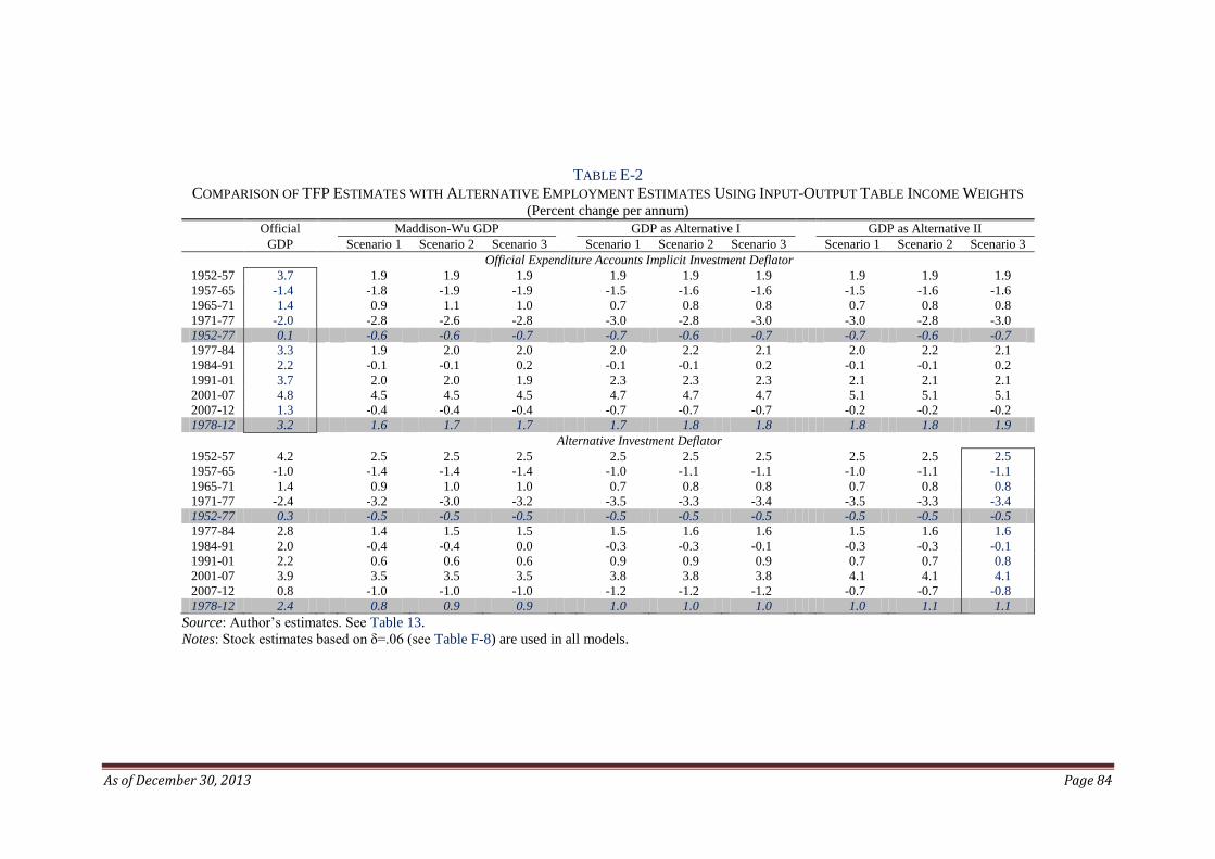
As of December 30, 2013 Page 84
TABLE E-2
COMPARISON OF TFP ESTIMATES WITH ALTERNATIVE EMPLOYMENT ESTIMATES USING INPUT-OUTPUT TABLE INCOME WEIGHTS (Percent change per annum)
Official Maddison-Wu GDP GDP as Alternative I GDP as Alternative II
GDP Scenario 1 Scenario 2 Scenario 3 Scenario 1 Scenario 2 Scenario 3 Scenario 1 Scenario 2 Scenario 3
Official Expenditure Accounts Implicit Investment Deflator
1952-57 3.7 1.9 1.9 1.9 1.9 1.9 1.9 1.9 1.9 1.9
1957-65 -1.4 -1.8 -1.9 -1.9 -1.5 -1.6 -1.6 -1.5 -1.6 -1.6
1965-71 1.4 0.9 1.1 1.0 0.7 0.8 0.8 0.7 0.8 0.8
1971-77 -2.0 -2.8 -2.6 -2.8 -3.0 -2.8 -3.0 -3.0 -2.8 -3.0
1952-77 0.1 -0.6 -0.6 -0.7 -0.7 -0.6 -0.7 -0.7 -0.6 -0.7
1977-84 3.3 1.9 2.0 2.0 2.0 2.2 2.1 2.0 2.2 2.1
1984-91 2.2 -0.1 -0.1 0.2 -0.1 -0.1 0.2 -0.1 -0.1 0.2
1991-01 3.7 2.0 2.0 1.9 2.3 2.3 2.3 2.1 2.1 2.1
2001-07 4.8 4.5 4.5 4.5 4.7 4.7 4.7 5.1 5.1 5.1
2007-12 1.3 -0.4 -0.4 -0.4 -0.7 -0.7 -0.7 -0.2 -0.2 -0.2
1978-12 3.2 1.6 1.7 1.7 1.7 1.8 1.8 1.8 1.8 1.9
Alternative Investment Deflator
1952-57 4.2 2.5 2.5 2.5 2.5 2.5 2.5 2.5 2.5 2.5
1957-65 -1.0 -1.4 -1.4 -1.4 -1.0 -1.1 -1.1 -1.0 -1.1 -1.1
1965-71 1.4 0.9 1.0 1.0 0.7 0.8 0.8 0.7 0.8 0.8
1971-77 -2.4 -3.2 -3.0 -3.2 -3.5 -3.3 -3.4 -3.5 -3.3 -3.4
1952-77 0.3 -0.5 -0.5 -0.5 -0.5 -0.5 -0.5 -0.5 -0.5 -0.5
1977-84 2.8 1.4 1.5 1.5 1.5 1.6 1.6 1.5 1.6 1.6
1984-91 2.0 -0.4 -0.4 0.0 -0.3 -0.3 -0.1 -0.3 -0.3 -0.1
1991-01 2.2 0.6 0.6 0.6 0.9 0.9 0.9 0.7 0.7 0.8
2001-07 3.9 3.5 3.5 3.5 3.8 3.8 3.8 4.1 4.1 4.1
2007-12 0.8 -1.0 -1.0 -1.0 -1.2 -1.2 -1.2 -0.7 -0.7 -0.8
1978-12 2.4 0.8 0.9 0.9 1.0 1.0 1.0 1.0 1.1 1.1
Source: Author’s estimates. See Table 13.
Notes: Stock estimates based on δ=.06 (see Table F-8) are used in all models.

As of December 30, 2013 Page 85
TABLE F-1
ALTERNATIVE ESTIMATES OF CHINESE EMPLOYMENT, 1949-2012 (Mid-year estimates in thousands)
Total Agriculture Industry Construction
Services
Of which: “Non-
material”
1949 182,413 161,454 5,818 1,250 13,892 9,084
1950 190,647 166,485 7,213 1,599 15,351 9,303
1951 201,402 171,673 8,942 2,045 18,742 11,135
1952 209,909 173,530 11,323 2,563 22,494 12,392
1953 215,165 175,320 13,099 3,131 23,615 12,036
1954 220,443 179,490 14,373 3,612 22,968 11,991
1955 224,788 183,715 14,506 4,469 22,098 11,646
1956 230,480 185,680 13,874 8,031 22,895 12,292
1957 237,358 189,265 13,877 9,173 25,043 13,447
1958 254,593 173,995 29,081 17,009 34,508 20,401
1959 266,265 158,805 36,482 25,908 45,070 29,670
1960 262,821 166,435 29,298 18,272 48,816 33,637
1961 260,239 183,815 26,012 8,828 41,584 27,384
1962 260,765 205,115 19,644 4,931 31,075 18,444
1963 266,439 216,210 16,686 3,799 29,744 17,538
1964 276,050 223,835 16,637 4,468 31,110 18,744
1965 286,742 230,985 17,616 5,339 32,802 20,194
1966 297,452 238,465 19,011 6,029 33,947 21,069
1967 308,329 247,310 20,030 6,275 34,714 21,450
1968 319,040 256,140 20,620 6,400 35,880 22,003
1969 331,262 265,900 22,287 6,578 36,497 22,326
1970 344,018 274,640 25,869 6,871 36,638 22,371
1971 358,581 281,040 32,209 7,074 38,258 22,731
1972 370,761 283,400 39,602 7,064 40,696 23,385
1973 381,242 285,700 45,919 7,133 42,490 23,868
1974 394,449 290,375 52,007 7,329 44,738 24,444
1975 407,958 293,370 59,219 7,750 47,618 25,027
1976 420,914 294,495 67,807 8,301 50,311 25,383
1977 432,582 293,915 75,095 9,089 54,482 27,106
1978 445,504 288,285 86,746 9,340 61,134 31,203
1979 460,542 284,750 99,160 9,433 67,199 34,474
1980 479,117 288,775 107,931 10,251 72,161 36,090
1981 500,900 294,495 117,466 10,933 78,006 38,119
1982 519,149 303,180 122,445 11,829 81,695 39,252
1983 533,197 310,050 124,579 13,313 85,256 40,663
1984 546,716 310,095 126,684 16,283 93,653 45,372
1985 560,242 309,990 127,668 20,603 101,981 49,345
1986 572,087 311,925 129,841 23,989 106,332 50,997
1987 582,424 314,585 131,732 26,143 109,965 53,441
1988 598,148 319,555 135,171 27,791 115,631 56,273
1989 619,076 327,365 141,914 28,128 121,669 58,515
1990 637,075 338,549 143,501 27,729 127,295 57,685
1991 651,200 347,175 141,851 27,847 134,327 64,237
1992 658,215 349,206 141,634 28,818 138,557 71,912
1993 664,800 345,798 140,787 31,708 146,506 78,575
1994 671,315 339,337 139,894 34,365 157,719 86,440
1995 677,600 332,374 138,932 35,646 170,648 93,734
1996 685,075 326,860 138,885 37,411 181,919 100,071
1997 693,850 326,475 139,237 39,324 188,814 104,182
1998 702,285 331,001 136,801 41,908 192,576 108,424
1999 710,155 338,301 131,944 44,289 195,621 111,638
2000 717,395 345,388 126,843 45,547 199,617 115,690
2001 725,550 351,502 123,300 46,795 203,953 121,001
2002 733,825 357,591 119,271 47,248 209,716 125,452
2003 740,860 359,838 118,925 45,101 216,996 130,245
2004 748,160 354,037 126,439 41,845 225,840 137,302
2005 755,125 341,883 135,690 42,210 235,342 146,719
2006 761,125 327,599 144,512 45,484 243,531 155,020
2007 766,950 314,281 154,183 49,084 249,402 160,451
2008 772,350 304,065 161,319 51,887 255,078 164,997
2009 777,375 294,742 163,106 55,833 263,694 171,505
2010 781,377 284,509 165,152 61,010 270,706 177,237
2011 784,427 272,623 169,610 64,169 278,025 183,427
2012 787,513 261,835 174,520 66,267 284,890 189,426
Sources & Notes: See Section 4, Scenario 2/3.

As of December 30, 2013 Page 86
TABLE F-2
FULL-TIME-EQUIVALENT MEASURE OF CHINESE EMPLOYMENT, 1949-2012 (Mid-year estimates in thousands)
Total Agriculture Industry Construction
Services
Of which: “Non-
material”
1949 194,064 170,201 7,088 1,317 15,458 10,108
1950 201,728 175,365 7,597 1,684 17,081 10,352
1951 212,737 180,341 9,393 2,148 20,854 12,390
1952 219,289 179,866 11,737 2,657 25,029 13,789
1953 224,110 181,071 13,529 3,233 26,277 13,392
1954 228,950 185,378 14,114 3,902 25,557 13,343
1955 244,142 200,303 14,378 4,872 24,588 12,959
1956 257,008 208,367 14,154 9,012 25,476 13,677
1957 265,299 212,390 14,750 10,294 27,865 14,963
1958 295,726 203,439 34,002 19,888 38,397 22,700
1959 321,708 194,962 44,789 31,807 50,151 33,015
1960 281,791 176,909 31,142 19,422 54,319 37,429
1961 277,496 195,382 26,459 9,383 46,271 30,471
1962 277,891 218,023 20,050 5,241 34,578 20,523
1963 295,000 240,583 17,093 4,227 33,097 19,515
1964 305,768 249,067 17,112 4,972 34,616 20,857
1965 317,669 257,023 18,206 5,941 36,500 22,471
1966 329,529 265,347 19,700 6,708 37,774 23,444
1967 341,597 275,189 20,799 6,983 38,627 23,868
1968 353,477 285,014 21,417 7,122 39,925 24,484
1969 366,945 295,874 23,141 7,319 40,611 24,842
1970 380,847 305,599 26,833 7,646 40,768 24,893
1971 406,112 321,753 33,132 8,073 43,154 25,495
1972 429,277 333,826 40,624 8,266 46,562 26,439
1973 451,222 346,255 47,080 8,560 49,327 27,201
1974 477,115 362,085 53,284 9,019 52,725 28,080
1975 503,733 376,386 60,544 9,781 57,021 28,980
1976 529,806 388,742 69,068 10,744 61,252 29,627
1977 554,972 399,182 76,335 12,064 67,390 31,891
1978 579,908 402,844 87,676 12,713 76,674 37,005
1979 607,452 409,397 99,345 13,168 85,542 41,210
1980 638,954 427,175 103,673 14,674 93,432 43,487
1981 665,358 435,637 112,780 15,650 101,291 46,065
1982 689,392 448,484 117,673 16,933 106,302 47,541
1983 708,789 457,822 120,543 19,012 111,411 49,496
1984 726,452 457,134 123,451 23,198 122,668 55,449
1985 744,858 456,294 125,334 29,284 133,946 60,456
1986 761,247 458,508 128,249 34,019 140,470 63,048
1987 775,380 461,819 130,938 36,990 145,634 66,400
1988 794,190 469,210 133,731 39,239 152,010 69,244
1989 817,611 479,889 139,479 39,578 158,665 71,232
1990 838,553 494,425 140,271 38,793 165,064 69,631
1991 857,525 504,200 139,189 38,973 175,163 78,633
1992 865,276 504,223 139,359 40,304 181,390 89,296
1993 872,587 496,246 139,002 44,273 193,066 98,986
1994 879,132 483,670 138,511 47,858 209,093 110,269
1995 884,341 469,915 137,937 49,459 227,030 120,391
1996 892,162 460,861 137,519 52,049 241,734 128,400
1997 902,745 459,578 137,589 54,888 250,690 133,527
1998 914,467 465,652 134,713 58,700 255,401 138,849
1999 927,474 476,010 129,642 62,268 259,554 142,424
2000 939,573 486,394 124,389 64,290 264,500 146,901
2001 929,629 477,678 122,199 64,849 264,903 150,220
2002 919,908 468,943 119,461 64,285 267,218 152,275
2003 907,328 455,372 120,381 60,248 271,327 154,569
2004 893,462 432,349 129,346 54,880 276,886 159,314
2005 880,092 402,894 140,285 54,351 282,562 166,446
2006 867,407 372,547 150,993 57,501 286,367 171,945
2007 856,084 344,892 162,809 60,923 287,461 174,002
2008 845,698 322,002 172,154 63,231 288,312 174,944
2009 836,179 301,204 175,909 66,801 292,265 177,792
2010 826,398 280,569 180,009 71,666 294,154 179,640
2011 816,396 259,437 186,831 74,006 296,122 181,771
2012 807,158 240,450 194,282 75,035 297,392 183,532
Sources & Notes: See Section 4, “Hours worked”.

As of December 30, 2013 Page 87
TABLE F-3
OFFICIAL ESTIMATES OF CHINESE EMPLOYMENT, 1952-2012 (End-year estimates in thousands)
Total Agriculture
Industry &
Construction Services
1952 216,293 179,494 15,869 20,930
1953 222,168 183,291 17,713 21,164
1954 226,334 187,464 18,852 20,018
1955 242,400 202,707 19,408 20,285
1956 256,519 208,097 26,101 22,321
1957 265,770 216,682 23,273 25,815
1958 308,734 181,113 82,734 44,887
1959 316,149 199,756 66,319 50,073
1960 277,453 180,868 43,708 52,877
1961 272,515 209,897 29,382 33,237
1962 275,991 226,149 21,189 28,653
1963 294,964 244,422 21,211 29,331
1964 307,178 253,713 22,843 30,622
1965 317,554 260,334 25,330 31,891
1966 330,139 270,359 27,421 32,358
1967 341,370 280,018 28,104 33,248
1968 353,576 290,010 28,971 34,595
1969 367,962 301,738 31,974 34,250
1970 381,037 309,461 37,049 34,528
1971 403,426 325,107 41,851 36,468
1972 415,653 333,155 44,798 37,700
1973 435,189 349,734 47,111 38,344
1974 454,343 364,336 49,477 40,530
1975 474,644 377,913 54,102 42,630
1976 493,517 388,656 58,840 46,021
1977 511,737 398,483 61,229 52,025
1978 529,588 395,697 72,561 61,331
1979 552,314 411,669 74,744 65,902
1980 582,789 430,792 76,519 75,478
1981 600,977 440,481 79,416 81,080
1982 622,646 456,487 83,026 83,133
1983 637,615 459,978 87,196 90,440
1984 658,514 455,048 97,637 105,829
1985 679,965 458,222 107,502 114,242
1986 702,294 459,427 117,452 125,416
1987 722,494 464,807 123,803 133,885
1988 741,591 473,519 128,083 139,988
1989 753,348 487,035 125,273 141,040
1990 879,618 568,311 143,982 167,324
1991 884,730 567,820 146,196 170,714
1992 888,570 558,779 150,346 179,446
1993 897,899 540,732 157,995 199,173
1994 903,740 522,073 162,774 218,893
1995 904,366 502,327 166,910 235,129
1996 908,406 490,945 173,164 244,296
1997 917,367 490,444 177,277 249,646
1998 931,921 494,873 178,450 258,597
1999 951,182 503,283 177,964 269,935
2000 971,461 507,570 176,780 287,111
2001 941,596 474,450 178,801 288,346
2002 915,186 443,629 174,278 297,278
2003 886,558 408,207 177,762 300,588
2004 857,043 366,477 186,941 303,625
2005 825,354 329,073 200,560 295,721
2006 829,736 311,721 213,366 304,648
2007 834,944 298,420 229,330 307,193
2008 838,801 288,386 235,119 315,296
2009 841,115 276,521 242,040 322,553
2010 838,628 263,751 251,275 323,601
2011 795,088 251,130 253,306 290,652
2012 799,783 243,377 261,529 294,877
Sources: Basic data are from various issues of China Statistical Yearbook and China Labor
Employment Yearbook, and cleaned up consistency in their own logic.

As of December 30, 2013 Page 88
TABLE F-4
CHINA’S SCHOOL GRADUATES BY LEVEL OF EDUCATION, 1949-2012 (Thousands)
Total Number
of Graduates
Of which:
Primary
Junior
Secondary
Senior
Secondary Tertiary
Other Types
1949 947 646 219 61 21 1950 1,097 783 234 62 18 1951 1,469 1,166 225 59 19 1952 1,743 1,490 185 36 32 1953 3,437 2,935 398 56 48 1954 4,016 3,325 576 68 47 0.1 1955 4,254 3,229 870 99 55 0.5 1956 5,054 4,051 785 154 63 0.5 1957 6,335 4,980 1,112 187 56 0.2 1958 7,448 6,063 1,116 197 72 0.4 1959 7,354 5,473 1,491 299 70 21 1960 9,335 7,340 1,422 288 136 149 1961 8,391 5,808 1,892 379 151 161 1962 7,837 5,590 1,584 441 177 45 1963 6,948 4,768 1,523 433 199 25 1964 7,682 5,674 1,386 367 204 51 1965 9,098 6,676 1,738 360 186 138 1966 11,046 9,005 1,620 280 141 1967 11,252 8,995 1,864 268 125 1968 20,416 14,282 5,190 794 150 1969 19,039 14,895 3,614 380 150 1970 23,493 16,525 6,189 676 103 1971 23,120 13,760 8,350 1,004 6 1972 26,680 14,149 10,355 2,159 17 1973 28,311 13,490 11,294 3,494 30 3 1974 30,041 15,210 10,606 4,179 43 3 1975 35,063 19,994 10,477 4,470 119 3 1976 42,279 24,895 12,060 5,172 149 3 1977 47,380 25,739 15,586 5,858 194 3 1978 46,800 22,879 16,926 6,827 165 3 1979 44,811 20,879 16,579 7,265 85 3 1980 36,573 20,533 9,648 6,162 147 83 1981 37,398 20,757 11,542 4,861 140 98 1982 34,708 20,689 10,321 3,106 457 135 1983 32,315 19,807 9,603 2,351 335 219 1984 31,917 19,950 9,504 1,898 287 278 1985 32,681 19,999 9,983 1,966 316 417 1986 33,948 20,161 10,570 2,240 393 584 1987 35,357 20,430 11,173 2,468 532 754 1988 34,749 19,303 11,572 2,506 553 815 1989 33,790 18,571 11,343 2,432 576 868 1990 33,564 18,631 11,091 2,330 614 898 1991 33,616 18,967 10,855 2,229 614 951 1992 33,588 18,724 11,023 2,261 604 976 1993 33,682 18,415 11,342 2,317 571 1,037 1994 34,342 18,996 11,526 2,093 637 1,090 1995 35,969 19,615 12,274 2,016 805 1,259 1996 36,439 19,341 12,790 2,049 839 1,420 1997 38,600 19,601 14,424 2,217 829 1,529 1998 41,987 21,174 15,802 2,518 830 1,663 1999 44,228 23,137 15,898 2,629 848 1,716 2000 46,034 24,192 16,071 3,015 950 1,806 2001 47,191 23,969 17,070 3,405 1,036 1,711 2002 48,991 23,519 18,799 3,838 1,337 1,499 2003 50,493 22,679 19,956 4,581 1,877 1,400 2004 51,388 21,352 20,704 5,469 2,391 1,472 2005 52,687 20,195 21,065 6,616 3,068 1,743 2006 52,795 19,285 20,624 7,271 3,775 1,840 2007 52,659 18,702 19,568 7,883 4,478 2,028 2008 52,978 18,650 18,629 8,361 5,119 2,219 2009 51,926 18,052 17,947 8,237 5,311 2,379 2010 50,959 17,396 17,486 7,944 5,754 2,379 2011 50,176 16,628 17,355 7,877 6,082 2,234 2012 49,421 16,416 16,867 7,656 6,247 2,235
Source: See Section 5 and Table 2.

As of December 30, 2013 Page 89
TABLE F-5
ESTIMATES OF PSE-BASED “HUMAN CAPITAL STOCK” IN CHINA, 1949-2012 (In million years, million persons and PSE years)
Years of
Schooling
(level mixed)
(ml. years)
PSE
Flows
(ml. years)
Net PSE
Stock
(ml. years)
Working-
Age
Population
(ml. years)
Net PSE
Stock Per
Working-
age Person
Numbers
Employed
(ml. years)
Net PSE
Stock Per
Employed
Person
1949 4.8 5.0 506.9 282.3 1.80 182.4 2.78 1950 5.7 5.8 507.7 286.3 1.77 190.6 2.66 1951 7.9 8.1 510.7 298.2 1.71 201.4 2.54 1952 9.7 9.9 515.5 312.5 1.65 209.9 2.46 1953 19.2 19.4 529.8 323.1 1.64 215.2 2.46 1954 22.1 22.4 546.9 331.2 1.65 220.4 2.48 1955 22.5 23.0 564.4 338.9 1.67 224.8 2.51 1956 27.4 27.9 586.7 346.3 1.69 230.5 2.55 1957 34.0 34.7 615.5 354.4 1.74 237.4 2.59 1958 40.6 41.3 650.7 363.3 1.79 254.6 2.56 1959 38.6 39.5 683.7 371.4 1.84 266.3 2.57 1960 50.2 51.3 728.1 376.4 1.93 262.8 2.77 1961 42.7 44.2 765.0 376.3 2.03 260.2 2.94 1962 40.5 41.8 799.1 374.1 2.14 260.8 3.06 1963 35.4 36.7 827.8 375.9 2.20 266.4 3.11 1964 40.3 41.5 861.0 382.4 2.25 276.0 3.12 1965 47.5 48.9 901.3 390.4 2.31 286.7 3.14 1966 60.3 61.3 953.6 399.4 2.39 297.5 3.21 1967 49.6 50.3 994.4 410.4 2.42 308.3 3.22 1968 63.4 64.3 1,048.7 422.2 2.48 319.0 3.29 1969 46.8 47.2 1,085.4 434.3 2.50 331.3 3.28 1970 36.6 37.1 1,111.6 447.1 2.49 344.0 3.23 1971 18.4 19.1 1,119.6 460.3 2.43 357.5 3.13 1972 20.4 21.3 1,129.7 473.2 2.39 367.5 3.07 1973 41.8 44.0 1,162.4 485.4 2.39 375.7 3.09 1974 60.5 62.8 1,213.6 496.8 2.44 386.4 3.14 1975 110.1 114.8 1,316.3 507.3 2.59 397.3 3.31 1976 176.5 184.6 1,487.7 518.4 2.87 407.5 3.65 1977 219.2 229.1 1,701.8 531.7 3.20 416.4 4.09 1978 208.9 219.9 1,904.7 546.1 3.49 426.3 4.47 1979 197.1 208.2 2,093.9 560.4 3.74 438.1 4.78 1980 171.3 179.3 2,252.2 574.9 3.92 453.0 4.97 1981 174.5 182.4 2,412.1 590.1 4.09 470.8 5.12 1982 166.7 173.3 2,561.3 606.9 4.22 490.1 5.23 1983 156.7 162.5 2,698.2 625.6 4.31 508.4 5.31 1984 155.9 161.2 2,832.4 645.3 4.39 528.1 5.36 1985 158.4 164.1 2,968.2 665.4 4.46 551.0 5.39 1986 162.7 169.0 3,107.5 684.7 4.54 572.1 5.43 1987 167.9 174.9 3,251.3 702.5 4.63 592.3 5.49 1988 162.7 170.8 3,389.6 719.2 4.71 613.8 5.52 1989 157.7 167.4 3,523.1 734.7 4.80 632.8 5.57 1990 157.2 165.0 3,652.9 749.2 4.88 642.7 5.68 1991 158.4 166.0 3,782.4 762.5 4.96 651.2 5.81 1992 157.6 164.3 3,908.9 774.3 5.05 658.2 5.94 1993 156.9 165.2 4,035.0 784.9 5.14 664.8 6.07 1994 160.7 172.9 4,167.6 795.0 5.24 671.3 6.21 1995 167.6 180.0 4,305.9 804.5 5.35 677.6 6.35 1996 168.3 179.2 4,442.0 813.7 5.46 685.1 6.48 1997 175.5 185.3 4,582.8 823.3 5.57 693.9 6.60 1998 190.4 202.3 4,739.3 833.7 5.68 702.3 6.75 1999 203.1 217.8 4,909.7 843.2 5.82 710.2 6.91 2000 211.8 228.4 5,089.1 858.9 5.93 717.4 7.09 2001 214.7 230.9 5,269.1 882.1 5.97 725.6 7.26 2002 219.0 241.4 5,457.8 897.3 6.08 733.8 7.44 2003 221.5 247.6 5,650.8 903.6 6.25 740.9 7.63 2004 220.8 248.0 5,842.3 911.1 6.41 748.2 7.81 2005 221.8 254.6 6,038.5 923.9 6.54 755.1 8.00 2006 220.2 258.4 6,236.4 939.1 6.64 761.1 8.19 2007 218.7 263.6 6,437.7 950.4 6.77 767.0 8.39 2008 220.2 265.2 6,638.5 958.5 6.93 772.4 8.60 2009 215.4 262.4 6,834.6 966.7 7.07 777.4 8.79 2010 211.0 253.8 7,020.0 979.0 7.17 781.4 8.98 2011 206.6 242.1 7,191.9 994.1 7.23 784.4 9.17 2012 203.9 232.6 7,352.6 1,002.1 7.34 787.5 9.34
Source: See Section 5 and Table 2.
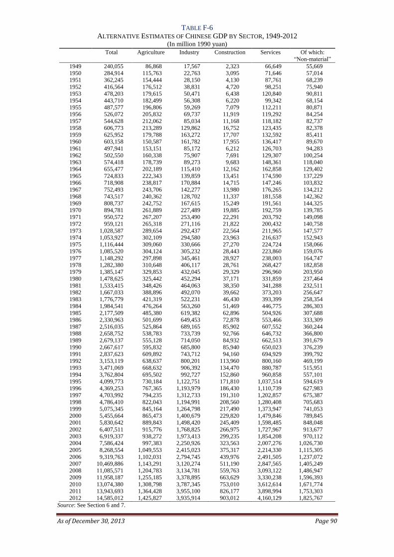
As of December 30, 2013 Page 90
TABLE F-6
ALTERNATIVE ESTIMATES OF CHINESE GDP BY SECTOR, 1949-2012 (In million 1990 yuan)
Total
Agriculture
Industry
Construction
Services
Of which:
“Non-material”
1949 240,055 86,868 17,567 2,323 66,649 55,669
1950 284,914 115,763 22,763 3,095 71,646 57,014
1951 362,245 154,444 28,150 4,130 87,761 68,239
1952 416,564 176,512 38,831 4,720 98,251 75,940
1953 478,203 179,615 50,471 6,438 120,840 90,811
1954 443,710 182,499 56,308 6,220 99,342 68,154
1955 487,577 196,806 59,269 7,079 112,211 80,871
1956 526,072 205,832 69,737 11,919 119,292 84,254
1957 544,628 212,062 85,034 11,168 118,182 82,737
1958 606,773 213,289 129,862 16,752 123,435 82,378
1959 625,952 179,788 163,272 17,707 132,592 85,411
1960 603,158 150,587 161,782 17,955 136,417 89,670
1961 497,941 153,151 85,172 6,212 126,703 94,283
1962 502,550 160,338 75,907 7,691 129,307 100,254
1963 574,418 178,739 89,273 9,683 148,361 118,040
1964 655,477 202,189 115,410 12,162 162,858 129,402
1965 724,833 222,343 139,859 13,451 174,590 137,229
1966 718,908 238,817 170,884 14,715 147,246 103,832
1967 752,493 243,706 142,277 13,980 176,265 134,212
1968 743,517 240,362 128,702 11,337 181,558 142,362
1969 808,737 242,752 167,615 15,249 191,561 144,325
1970 894,781 261,889 227,489 19,885 192,759 139,785
1971 950,572 267,207 253,490 22,291 203,792 149,098
1972 959,121 265,318 271,116 21,822 200,432 140,758
1973 1,028,587 289,654 292,437 22,564 211,965 147,577
1974 1,053,927 302,109 294,580 23,963 216,637 152,943
1975 1,116,444 309,060 330,666 27,270 224,724 158,066
1976 1,085,520 304,124 305,232 28,443 223,860 159,076
1977 1,148,292 297,898 345,461 28,927 238,003 164,747
1978 1,282,380 310,648 406,117 28,761 268,427 182,858
1979 1,385,147 329,853 432,045 29,329 296,960 203,950
1980 1,478,625 325,442 452,294 37,171 331,859 237,464
1981 1,533,415 348,426 464,063 38,350 341,288 232,511
1982 1,667,033 388,896 492,070 39,662 373,203 256,647
1983 1,776,779 421,319 522,231 46,430 393,399 258,354
1984 1,984,541 476,264 563,260 51,469 446,775 286,303
1985 2,177,509 485,380 619,382 62,896 504,926 307,688
1986 2,330,963 501,699 649,453 72,878 553,466 333,309
1987 2,516,035 525,864 689,165 85,902 607,552 360,244
1988 2,658,752 538,783 733,739 92,766 646,732 366,800
1989 2,679,137 555,128 714,050 84,932 662,513 391,679
1990 2,667,617 595,832 685,800 85,940 650,023 376,239
1991 2,837,623 609,892 743,712 94,160 694,929 399,792
1992 3,153,119 638,637 800,201 113,960 800,160 469,199
1993 3,471,069 668,632 906,392 134,470 880,787 515,951
1994 3,762,804 695,502 992,727 152,860 960,858 557,101
1995 4,099,773 730,184 1,122,751 171,810 1,037,514 594,619
1996 4,369,253 767,365 1,193,979 186,430 1,110,739 627,983
1997 4,703,992 794,235 1,312,733 191,310 1,202,857 675,387
1998 4,786,410 822,043 1,194,991 208,560 1,280,408 705,683
1999 5,075,345 845,164 1,264,798 217,490 1,373,947 741,053
2000 5,455,664 865,473 1,400,679 229,820 1,479,846 789,845
2001 5,830,642 889,843 1,498,420 245,409 1,598,485 848,048
2002 6,407,511 915,776 1,768,825 266,975 1,727,967 913,677
2003 6,919,337 938,272 1,973,413 299,235 1,854,208 970,112
2004 7,586,424 997,383 2,250,926 323,563 2,007,276 1,026,730
2005 8,268,554 1,049,553 2,415,023 375,317 2,214,330 1,115,305
2006 9,319,763 1,102,031 2,794,745 439,976 2,491,505 1,237,072
2007 10,469,886 1,143,291 3,120,274 511,190 2,847,565 1,405,249
2008 11,085,571 1,204,783 3,134,781 559,763 3,093,122 1,486,947
2009 11,958,187 1,255,185 3,378,895 663,629 3,330,238 1,596,393
2010 13,074,380 1,308,798 3,787,345 753,010 3,612,614 1,671,774
2011 13,943,693 1,364,428 3,955,100 826,177 3,898,994 1,753,303
2012 14,585,012 1,425,827 3,935,914 903,012 4,160,129 1,825,767
Source: See Section 6 and 7.
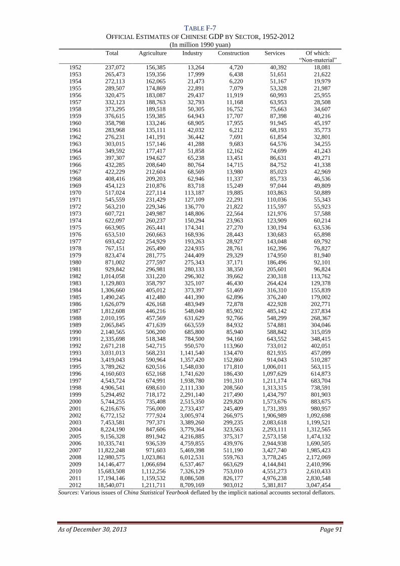
As of December 30, 2013 Page 91
TABLE F-7
OFFICIAL ESTIMATES OF CHINESE GDP BY SECTOR, 1952-2012 (In million 1990 yuan)
Total
Agriculture
Industry
Construction
Services
Of which:
“Non-material”
1952 237,072 156,385 13,264 4,720 40,392 18,081
1953 265,473 159,356 17,999 6,438 51,651 21,622
1954 272,113 162,065 21,473 6,220 51,167 19,979
1955 289,507 174,869 22,891 7,079 53,328 21,987
1956 320,475 183,087 29,437 11,919 60,993 25,955
1957 332,123 188,763 32,793 11,168 63,953 28,508
1958 373,295 189,518 50,305 16,752 75,663 34,607
1959 376,615 159,385 64,943 17,707 87,398 40,216
1960 358,798 133,246 68,905 17,955 91,945 45,197
1961 283,968 135,111 42,032 6,212 68,193 35,773
1962 276,231 141,191 36,442 7,691 61,854 32,801
1963 303,015 157,146 41,288 9,683 64,576 34,255
1964 349,592 177,417 51,858 12,162 74,699 41,243
1965 397,307 194,627 65,238 13,451 86,631 49,271
1966 432,285 208,640 80,764 14,715 84,752 41,338
1967 422,229 212,604 68,569 13,980 85,023 42,969
1968 408,416 209,203 62,946 11,337 85,733 46,536
1969 454,123 210,876 83,718 15,249 97,044 49,809
1970 517,024 227,114 113,187 19,885 103,863 50,889
1971 545,559 231,429 127,109 22,291 110,036 55,343
1972 563,210 229,346 136,770 21,822 115,597 55,923
1973 607,721 249,987 148,806 22,564 121,976 57,588
1974 622,097 260,237 150,294 23,963 123,909 60,214
1975 663,905 265,441 174,341 27,270 130,194 63,536
1976 653,510 260,663 168,936 28,443 130,683 65,898
1977 693,422 254,929 193,263 28,927 143,048 69,792
1978 767,151 265,490 224,935 28,761 162,396 76,827
1979 823,474 281,775 244,409 29,329 174,950 81,940
1980 871,002 277,597 275,343 37,171 186,496 92,101
1981 929,842 296,981 280,133 38,350 205,601 96,824
1982 1,014,058 331,220 296,302 39,662 230,318 113,762
1983 1,129,803 358,797 325,107 46,430 264,424 129,378
1984 1,306,660 405,012 373,397 51,469 316,310 155,839
1985 1,490,245 412,480 441,390 62,896 376,240 179,002
1986 1,626,079 426,168 483,949 72,878 422,928 202,771
1987 1,812,608 446,216 548,040 85,902 485,142 237,834
1988 2,010,195 457,569 631,629 92,766 548,299 268,367
1989 2,065,845 471,639 663,559 84,932 574,881 304,046
1990 2,140,565 506,200 685,800 85,940 588,842 315,059
1991 2,335,698 518,348 784,500 94,160 643,552 348,415
1992 2,671,218 542,715 950,570 113,960 733,012 402,051
1993 3,031,013 568,231 1,141,540 134,470 821,935 457,099
1994 3,419,043 590,964 1,357,420 152,860 914,043 510,287
1995 3,789,262 620,516 1,548,030 171,810 1,006,011 563,115
1996 4,160,603 652,168 1,741,620 186,430 1,097,629 614,873
1997 4,543,724 674,991 1,938,780 191,310 1,211,174 683,704
1998 4,906,541 698,610 2,111,330 208,560 1,313,315 738,591
1999 5,294,492 718,172 2,291,140 217,490 1,434,797 801,903
2000 5,744,255 735,408 2,515,350 229,820 1,573,676 883,675
2001 6,216,676 756,000 2,733,437 245,409 1,731,393 980,957
2002 6,772,152 777,924 3,005,974 266,975 1,906,989 1,092,698
2003 7,453,581 797,371 3,389,260 299,235 2,083,618 1,199,521
2004 8,224,190 847,606 3,779,364 323,563 2,293,111 1,312,565
2005 9,156,328 891,942 4,216,885 375,317 2,573,158 1,474,132
2006 10,335,741 936,539 4,759,855 439,976 2,944,938 1,690,505
2007 11,822,248 971,603 5,469,398 511,190 3,427,740 1,985,423
2008 12,980,575 1,023,861 6,012,531 559,763 3,778,245 2,172,069
2009 14,146,477 1,066,694 6,537,467 663,629 4,144,841 2,410,996
2010 15,683,508 1,112,256 7,326,129 753,010 4,551,273 2,610,433
2011 17,194,146 1,159,532 8,086,508 826,177 4,976,238 2,830,548
2012 18,540,071 1,211,711 8,709,169 903,012 5,381,817 3,047,454
Sources: Various issues of China Statistical Yearbook deflated by the implicit national accounts sectoral deflators.
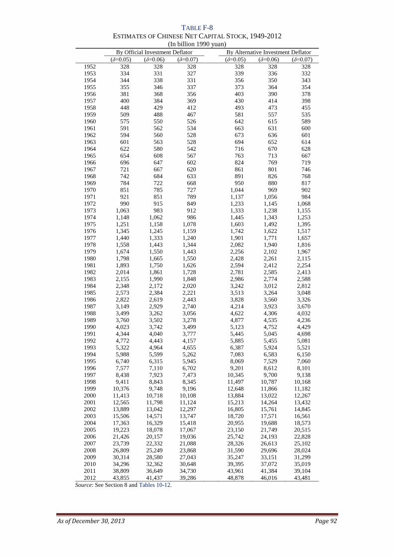
As of December 30, 2013 Page 92
TABLE F-8
ESTIMATES OF CHINESE NET CAPITAL STOCK, 1949-2012 (In billion 1990 yuan)
By Official Investment Deflator By Alternative Investment Deflator
(δ=0.05) (δ=0.06) (δ=0.07) (δ=0.05) (δ=0.06) (δ=0.07)
1952 328 328 328 328 328 328
1953 334 331 327 339 336 332
1954 344 338 331 356 350 343
1955 355 346 337 373 364 354
1956 381 368 356 403 390 378
1957 400 384 369 430 414 398
1958 448 429 412 493 473 455
1959 509 488 467 581 557 535
1960 575 550 526 642 615 589
1961 591 562 534 663 631 600
1962 594 560 528 673 636 601
1963 601 563 528 694 652 614
1964 622 580 542 716 670 628
1965 654 608 567 763 713 667
1966 696 647 602 824 769 719
1967 721 667 620 861 801 746
1968 742 684 633 891 826 768
1969 784 722 668 950 880 817
1970 851 785 727 1,044 969 902
1971 921 851 789 1,137 1,056 984
1972 990 915 849 1,233 1,145 1,068
1973 1,063 983 912 1,333 1,238 1,155
1974 1,148 1,062 986 1,445 1,343 1,253
1975 1,251 1,158 1,078 1,603 1,492 1,395
1976 1,345 1,245 1,159 1,742 1,622 1,517
1977 1,440 1,333 1,240 1,901 1,771 1,657
1978 1,558 1,443 1,344 2,082 1,940 1,816
1979 1,674 1,550 1,443 2,256 2,102 1,967
1980 1,798 1,665 1,550 2,428 2,261 2,115
1981 1,893 1,750 1,626 2,594 2,412 2,254
1982 2,014 1,861 1,728 2,781 2,585 2,413
1983 2,155 1,990 1,848 2,986 2,774 2,588
1984 2,348 2,172 2,020 3,242 3,012 2,812
1985 2,573 2,384 2,221 3,513 3,264 3,048
1986 2,822 2,619 2,443 3,828 3,560 3,326
1987 3,149 2,929 2,740 4,214 3,923 3,670
1988 3,499 3,262 3,056 4,622 4,306 4,032
1989 3,760 3,502 3,278 4,877 4,535 4,236
1990 4,023 3,742 3,499 5,123 4,752 4,429
1991 4,344 4,040 3,777 5,445 5,045 4,698
1992 4,772 4,443 4,157 5,885 5,455 5,081
1993 5,322 4,964 4,655 6,387 5,924 5,521
1994 5,988 5,599 5,262 7,083 6,583 6,150
1995 6,740 6,315 5,945 8,069 7,529 7,060
1996 7,577 7,110 6,702 9,201 8,612 8,101
1997 8,438 7,923 7,473 10,345 9,700 9,138
1998 9,411 8,843 8,345 11,497 10,787 10,168
1999 10,376 9,748 9,196 12,648 11,866 11,182
2000 11,413 10,718 10,108 13,884 13,022 12,267
2001 12,565 11,798 11,124 15,213 14,264 13,432
2002 13,889 13,042 12,297 16,805 15,761 14,845
2003 15,506 14,571 13,747 18,720 17,571 16,561
2004 17,363 16,329 15,418 20,955 19,688 18,573
2005 19,223 18,078 17,067 23,150 21,749 20,515
2006 21,426 20,157 19,036 25,742 24,193 22,828
2007 23,739 22,332 21,088 28,326 26,613 25,102
2008 26,809 25,249 23,868 31,590 29,696 28,024
2009 30,314 28,580 27,043 35,247 33,151 31,299
2010 34,296 32,362 30,648 39,395 37,072 35,019
2011 38,809 36,649 34,730 43,961 41,384 39,104
2012 43,855 41,437 39,286 48,878 46,016 43,481
Source: See Section 8 and Tables 10-12.

As of December 30, 2013 Page 93
REFERENCES
Adams, F. Gerard and Yimin Chen, “Skepticism about Chinese GDP growth – the
Chinese GDP elasticity of energy consumption”, Journal of Economic and
Social Measurement, 22, 231-240, 1996.
Bai, Chong-en, Chang-tai Hsieh and Yingi Qian (2007), “Return on Capital in China”,
Comparative Study (Bijiao), 28
Barro, R.J., & Lee, J. W. (1997). International measures of schooling years and
schooling quality. American Economic Review, Papers and Proceedings, 86(2),
218–223.
Barro, R.J., & Lee, J. W. (2000, April and August). International data on educational
attainment: updates and implications. CID Working Paper No. 42. Center for
International Development at Harvard University, Cambridge, MA.
Bergson, Abram (1961), Real National Income of Soviet Russia Since 1928
(Cambridge: Harvard University Press, 1961), 26-37.
Berndt, Ernst R. and Jack E. Triplett (eds.) (1990), Fifty Years of Economic
Measurement – The Jubilee of the Conference on Research in Income and
Wealth, Volume 54, National Bureau of Economic Research.
Borensztein, Eduardo and Jonathan D. Ostry, 1996 “Accounting for China’s Growth
Performance”, American Economic Review 86 (2), 224-28.
Bosworth, Barry and Susan M. Collins (2008), “Accounting for Growth: Comparing
China and India”, Journal of Economic Perspectives, Volume 22, Number 1:
45–66
Cao, Jing, Mun S. Ho, Dale W. Jorgenson, Ruoen Ren, Linlin Sun, Ximing Yue
(2009), “Industrial and aggregate measures of productivity growth in China,
1982–2000,” Review of Income and Wealth, Series 55, Special Issue 1, July
CASS (Chinese Academy of Social Sciences) and CA (Central Achieves) (1998),
Selected Economic Achieves of the People’s Republic of China: Infrastructural
Investment and Construction Volume, 1949-1952, China Urban Economic and
Social Press.
CEC (Commission of the European Communities), IMF, OECD, UN and the World
Bank, 1993, System of National Accounts, Brussels/Luxembourg, New York,
Paris, Washington, D.C.
CHIP (China Household Income Project), (1988, 1995, 2002 and 2007), China
Household Income Survey. Beijing: Institute of Economic Research, Chinese
Academy of Social Sciences
Chow, Gregory C. (1993). “Capital Formation and Economic Growth in China”,
Quarterly Journal of Economics 108 (3), 809-42.
Chow, Gregory C. (2006). New capital estimates for China: Comments. China
Economic Review, 17, 186–192
Chow, Gregory C. and Kui-Wai Li (2002), China’s Economic Growth: 1952–2010,
Economic Development and Cultural Change, 51: 247-256

As of December 30, 2013 Page 94
Dev Pant, Bishnu (ed.) (2007), The National Accounts of the People's Republic of
China: Measurement Issues, Recent Developments, and the Way Forward,
Asian Development Bank, Manila.
DFAIS (Department of Fixed Assets Investment Statistics, NBS), 1997, China Fixed
Assets Investment Statistical Yearbook 1950-1995, China Statistical Publishing
House, Beijing
DIS (Department of Industrial Statistics, NBS), (various issues) China Industrial
Economy Statistical Yearbook, China Statistical Publishing House, Beijing
DITS (Department of Industrial and Transportation Statistics, NBS), (various issues)
China Industrial Economy Statistical Yearbook, China Statistical Publishing
House, Beijing
DNEA (Department of National Economic Accounts, NBS) (1996), Input-Output
Table of China 1992, China Statistical Publishing House.
DNEA (Department of National Economic Accounts, NBS) (1997), The Gross
Domestic Product of China 1952-1995, Dongbei University of Finance and
Economic Press.
DNEA (Department of National Economic Accounts, NBS) (1999), Input-Output
Table of China 1997, China Statistical Publishing House.
DNEA (Department of National Economic Accounts, NBS) (2004), The Gross
Domestic Product of China 1996-2002, China Statistical Publishing House,
Beijing.
DNEA (Department of National Economic Accounts, NBS) (2005), Input-Output
Table of China 2002, China Statistical Publishing House.
DNEA (Department of National Economic Accounts, NBS) (2009), Input-Output
Table of China 2007, China Statistical Publishing House.
DNEA (Department of National Economic Accounts) (2007), Historical Data of
Gross Domestic Product of China, 1952-2004, China Statistical Publishing
House, Beijing.
DNEB (Department of National Economic Balance, State Statistical Bureau of China)
and ONIOS (Office of the National Input-Output Survey) (1991), Input-Output
Table of China 1987, China Statistical Publishing House, Beijing.
DSS (Department of Social Statistics, NBS) (1987), Zhongguo Laodong Gongzi
Tongji Ziliao [China labour and Wage Statistics] 1949-1985, China Statistical
Publishing House, Beijing.
DSS (Department of Social Statistics, NBS) (1989), Zhongguo Laodong Gongzi
Tongji Ziliao [China labour and Wage Statistics] 1949-1985, China Statistical
Publishing House, Beijing.
EC (Editorial Committee), 2002, New Handbook of Regular Data and Coefficients for
Assets Evaluation, Vol. 1, China Statistical Publishing House, Beijing.
Fan, Shanggen, Xiaobao Zhang, and Sherman Robinson (1999), “Past and Future
Sources of Growth for China,” EPTD Discussion Paper No. 53, International
Food Policy Research Institute, Washington, D.C.

As of December 30, 2013 Page 95
Field, R. M., Real Capital Formation in the People's Republic of China, 1952-73, in
Eckstein, A. (ed.), Quantitative Measures of China's Economic Output, pp. 194-
245, The University of Michigan Press, Ann Arbor, 1980
Felipe, Jesus, 1999, “Total Factor Productivity Growth in East Asia: A Critical
Survey”, Journal of Development Studies 35 (4), pp.1-41.
Gerschenkron, A., A Dollar Index of Soviet Machinery Output, 1927-28 to 1937,
Santa Monica CA, Rand Corporation, 1951.
Gollin, Douglas (2002), “Getting Income Shares Right,” Journal of Political Economy,
110, 458–475.
He, Feng, Chen Rong and He Lin (2003), “Estimation of China’s Capital Stock and
Analysis, The Economist (Jingji Xuejia), No. 5
He, Jianwu and Louis Kuijs (2007), “Rebalancing China’s economy—modeling a
policy package”, World Bank China Research Paper No. 7, Beijing
He, Juhuang (1992), “Estimation of China’s Fixed Assets”, Quantitative and
Technical Economy Research (Shuliang Jingji yu Jishu Jingji Yanjiu), No. 8
Ho, Mun S. and Dale W. Jorgenson, 2001, Productivity Growth in China, 1981-95,
mimeo, Kennedy School of Government, Harvard University, Cambridge, MA
Holz, Carsten A. (2006a), “China’s Reform Period Economic Growth: How Reliable
Are Angus Maddison’s Estimates?” The Review of Income and Wealth, March:
85-119
Holz, Carsten A. (2006b). New capital estimates for China. China Economic Review,
17, 142–185
Holz, Carsten A. (2006c). Response to Gregory C. Chow’s “New Capital Estimates
for China: Comments”. China Economic Review, 17, 193-197
Hu, Zuliu F. and Mohsin S. Khan, 1997, “Why is China growing so fast?”, IMF Staff
Papers, 44 (1), 103-131.
Huang, Yiping and Kunyu Tao (2010), “Factor Market Distortion and the Current
Account Surplus in China”, Asian Economic Papers, 9 (3)
Garnaut, Ross and Guonan, Ma (1993), “How Rich is China: Evidence from the Food
Economy,” The Australian Journal of Chinese Affairs, No. 30, pp. 121-146.
Geng, Nan and Papa N'Diaye (2012), “Determinants of Corporate Investment in
China: Evidence from Cross-Country Firm Level Data”, IMF Working Paper,
WP/12/80
Gerschenkron, Alexander. (1947), "The Soviet Indices of Industrial Production," The
Review of Economics and Statistics, XXXIV (Aug. 1947).
Gerschenkron, Alexander. 1951. A dollar index of Soviet machinery output, 1927-28
to 1937. Santa Monica, Calif.: Rand
Huang, Yongfeng, Ruoen Ren and Xiaosheng Liu (2002), “Estimation of Capital
Stock for Chinese Manufacturing by the Perpetual Inventory Method”, China
Economic Quarterly (Jingjixue Jikan), Vol. 1 (2), 377-396
Hulten, Charles R., and Frank C. Wykoff (1981), “The measurement of economic
depreciation”, in Charles R. Hulten (ed.), Depreciation, Inflation, and the

As of December 30, 2013 Page 96
Taxation of Income from Capital, 81-125, The Urban Institute Press,
Washington D.C.
IER (Institute of Economic Research, Hitotsubashi University) (1999), Post-War
Chinese Industrial Price Data, Hitotsubashi University.
IER (Institute of Economic Research, Hitotsubashi University) (2008), Supplementary
Chinese Price Data (PPIs) on 3-Digit Industries, Hitotsubashi University.
Jefferson, Gary H., Thomas G. Rawski and Yuxin Zheng, 1996, “Chinese Industrial
Productivity: Trends, Measurement Issues, and Recent Developments”, Journal
of Comparative Economics, 23: 146-80.
Jorgenson, Dale W. (1990), “Productivity and Economic Growth”, in Ernst R. Berndt
and Jack E. Triplett (eds.), Fifty Years of Economic Measurement – The Jubilee
of the Conference on Research in Income and Wealth, Volume 54, National
Bureau of Economic Research.
Jorgenson, Dale W., Frank Gollop and Barbara Fraumeni (1987), Productivity and
U.S. Economic Growth, Harvard University Press, Cambridge, MA
Kalirajan, K.P., M.B. Obwona, and S. Zhao, 1996, “A Decomposition of Total Factor
Productivity Growth: The Case of Chinese Agricultural Growth Before and
After Reforms”, American Journal of Agricultural Economics, 78, 331-38.
Keidel, Albert (1992), How Badly do China’s National Accounts Underestimate
China’s GNP? Rock Creek Research Inc. Paper E-8042
Keidel, Albert (2001), “China’s GDP Expenditure Accounts”, China Economic
Review, 12: 355-367.
Kim, J. I., and L. Lau, 1994. “The Sources of Economic Growth of the East Asian
Newly Industrialized Countries.” Journal of the Japanese and International
Economies 8:235-71.
King, Robert J. and Ross Levine (1994), “Capital Fundamentalism Economic
Development and Economic Growth.” Carnegie-Rochester Conference Series
on Public Policy 40 (June): 259-292.
Krugman, Paul (1994), “The Myth of Asia’s Miracle”, Foreign Affairs,
November/December: 62-78
Li, Jingwen, et al., 1992, “Productivity and China’s Economic Growth”, Economic
Studies Quarterly, 43 (4): 337-350
Li, Hongbin, and Li-An Zhou. 2005. “Political Turnover and Economic Performance:
The Incentive Role of Personnel Control in China.” Journal of Public Economics,
89(9–10): 1743–62.
Lin, Justin Yifu, Fang Cai and Zhou Li (1996), The China Miracle: Development
Strategy and Economic Reform, The Chinese University Press, Hong Kong
Liu, Ta-chung and Kung-chia, Yeh (1965), The Economy of the Chinese Mainland:
National Income and Economic Development, 1933-1959, Princeton University
Press.
Ma, Jun (1997), Intergovernmental Relations and Economic Management in China,
Macmillan Press.

As of December 30, 2013 Page 97
Maddison, Angus (1995), Monitoring the World Economy, 1820-1992, OECD
Development Centre, Paris.
Maddison, Angus (1998a), Chinese Economic Performance in the Long Run, OECD
Development Centre, Paris (available on www.ggdc.net/Maddison).
Maddison, Angus (1998b), “Measuring the Performance of a Communist Command
Economy: An Assessment of C.I.A. Estimates for the USSR”, Review of Income
and Wealth, September, pp. 307-325.
Maddison, Angus (2006), “Do Official Statistics Exaggerate Growth? A Reply to
Caersten Holz”, Review of Income and Wealth, March, pp. 121-6.
Maddison, Angus (2007), Chinese Economic Performance in the Long Run, 960-2030,
OECD, Paris.
Maddison, Angus and Harry X. Wu (2008), “Measuring China’s Economic
Performance”, with Angus Maddison, World Economics, Vol. 9 (2), April-June
Mao, Weining and Won W. Koo, 1997, “Productivity Growth, Technological
Progress, and Efficiency Change in Chinese Agriculture after Rural Economic
Reform: A DEA Approach”, China Economic Review, 8 (2): 157-74.
Meng, Xin, and Kidd, Michael P., 1997. Wage determination in China’s state sector in
the 1980s. Journal of Comparative Economics, 25 (3), 403–421.
Meng, Xin, Kailing Shen and Sen Xue, 2012. “Economic reform, education expansion,
and earnings inequality for urban males in China, 1988–2009”, Journal of
Comparative Economics, xx (x)
Ministry of Finance, 1992, Service Life of Industrial Fixed Assets, Appendix 1, in No.
574 Circular issued on 30 December, 1992.
NBS (National Bureau of Statistics, China) (various years), China Statistical
Yearbook, China Statistical Press, Beijing
NBS and MoL [National Bureau of Statistics and Ministry of Labour], 1994, Laodong
tongji Zhibiao Jieshi ji Wenjian Xiuanbian [Explanation of Labour Statistical
Indicators and Selected Documents]. Beijing: China Statistical Publishing
House.
Oi, Jean C. (1992), "Fiscal reform and the economic foundations of local state
corporatism in China," World Politics, 45: 99-126
Pack, H., 1993. “Technology Gaps between Industrial and Developing Countries: Are
there Dividends for Latecomers?” Proceedings of the World Bank Annual
Conference on Development Economics 1992. The World Bank.
Perkins, Dwight H. (1975), “Growth and Changing Structure of China’s Twentieth-
Century Economy”, in Perkins, D.H. (ed.), China’s Modern Economy in Historical
Perspective, Stanford University Press.
Perkins, Dwight H. and Thomas G. Rawski, (2008), “Forecasting China's Economic
Growth to 2025”, Chapter 20, in Loren Brandt, Thomas G. Rawski (eds.)
China's Great Economic Transformation, Cambridge University Press
Popov, Vladimir, (2007), “Shock Therapy versus Gradualism Reconsidered: Lessons
from Transition Economies after 15 Years of Reforms”, Comparative Economic
Studies, 49: 1-31.
As of December 30, 2013 Page 98
Qian, Yingyi, Gerard Roland, and Chenggang Xu. 2006. “Coordination and
Experimentation in M-Form and U-Form Organizations.” Journal of Political
Economy, 114(2): 366–402.
Qian, Yingyi, Gerard Roland, and Chenggang Xu. 2007. “Coordinating Changes in
Transition Economies.” In The Economics of Transition: The Fifth Nobel
Symposium in Economics, ed. Erik Berglöf and Gérard Roland, 518–46. New
York: Palgrave Macmillan.
Rawski, Thomas G. (1989), Economic Growth in Prewar China, University of
California Press, Berkeley
Rawski, Thomas G. (1993), “How fast has the Chinese industry grown?”, Policy
Research Working Paper, WPS 1194, Policy Research Department, World Bank,
Washington D.C.
Rawski, Thomas G. (2001), “What is Happening to China’s GDP Statistics?”, China
Economic Review, 12: 347-354
Rawski, Thomas G. (2008), Can China Sustain Rapid Growth Despite Flawed
Institutions? For The Sixth International Symposium of the Center for China-Us
Cooperation, University of Denver, May 30-31, 2008
Rawski, Thomas, and Robert W. Mead. (1998) “On the Trail of China’s Phantom
Farmers,” World Development, Vol. 26, No. 5, pp. 767-781
Ren, Ruoen (1997), China’s Economic Performance in International Perspective,
OECD, Paris.
Ren, Ruoen and Xiaosheng Liu (1997), “On the Estimation of China’s Capital Stock,”,
Quantitative and Technical Economy Research (Shuliang Jingji yu Jishu Jingji
Yanjiu), 1997 (1).
Ren, Ruoen and Linlin Sun (2007), “Total Factor Productivity Growth in China
Industries: 1981–2000,” Dale Jorgenson, Masahiro Kuroda and Kazuyuki
Motohashi (eds.), Productivity in Asia: Economic Growth and Competitiveness,
Cheltenham, UK and Northampton, MA, USA: Edward Elgar
SETC (State Economic and Trade Commission, China) (2000), Fifty Years of Chinese
Industry, China Economic Press, Beijing
Shiau, Allen (2004), “Has Chinese Government Overestimated China’s Economic
Growth?” in Yue, Ximing, Zhang Shuguang and Xu Xianchun (eds.), Studies
and Debates on the Rate of Growth of the Chinese Economy, CITIC Publishing
House, Beijing.
SSB (State Statistical Bureau, China), (various years), China Statistical Yearbook,
China Statistical Press, Beijing
SSB-Hitotsubashi University Institute of Economic Research (1997) The Historical
National Accounts of the People’s Republic of China, 1952-1995.
State Council, 1985, Probation Regulation on the Depreciation of Fixed Assets in
State-owned Enterprises, Circular No. 63, issued on 26 April, 1985
Sun, Linlin and Ren Ruoen (2003), “Estimates of Capital Input Index by Industries:
The People’s Republic of China (1980-1999)”, paper presented at the
International Comparison of the Productivity among Pan-Pacific Countries,
ICPA Project, No.5
As of December 30, 2013 Page 99
Tang, Zhihong (1999), “Estimation of China’s Average Profitability”, Economic
Research Journal (Jingji Yangjiu), No. 5
TCB (The Conference Board) (2013), The Conference Board Total Economy
Database™, http://www.conference-board.org/data/economydatabase
van Ark, Bart. (1996), “Sectoral Growth Accounting and Structural Change in
Postwar Europe” pp. 84-164 in B. van Ark & N. Crafts, Quantitative Aspects of
post-war European Economic Growth, Cambridge University Press.
Walder, Andrew G. (1995), “Local governments as industrial firms: an organizational
analysis of China's transitional economy,” American Journal of Sociology, 101 (2):
263-301.
Wang, Xiaolu and Gang Fan (2000), Sustainability of The Chinese Economy –– A
Centennially Retrospective and Prospective View (Zhongguo Jingji Zengzhang
de Kechixuxing –– Kua Shiji de Huigu yu Zhanwang), Economic Science Press
Wang, Yan and Yudong Yao (2002), “Sources of China’s Economic Growth, 1952–
99: Incorporating Human Capital Accumulation,” China Economic Review,
Wang, Lili and Adam Szirmai (2012), “Capital inputs in the Chinese economy:
Estimates for the total economy, industry and manufacturing,” China Economic
Review, 23: 81-104
Woo, Wing Thye, 1998, “Chinese Economic Growth: Sources and Prospects”, in M.
Fouquin and F. Lemonie (eds.) The Chinese Economy, Economica Ltd., Paris
World Bank (1994), China GNP per Capita, Report No. 13580-CHA, Country
Operations Division, China and Mongolia Department, World Bank
Wu, Harry X. (1994), “The Rural Industrial Workforce”, in C. Findlay, A. Watson
and H. X. Wu (eds.), Rural Enterprises in China, Macmillan Press, London, pp.
117-147
Wu, Harry X. (1997), “Reconstructing Chinese GDP According to the National
Accounts Concept of Value Added: the Industrial Sector”, COPPAA Working
Paper, 4, Centre for the Study of Australia-Asian Relations, Griffith University,
Brisbane.
Wu, Harry X. (2000), “Measuring China’s GDP level and Growth Performance:
Alternative Estimates and the Implications”, Review of Income and Wealth,
Series 46 (4): 475-499.
Wu, Harry X. (2002a), “How Fast Has Chinese Industry Grown? – Measuring the
Real Output of Chinese Industry, 1949-97”, Review of Income and Wealth, June,
pp. 179-204.
Wu, Harry X. (2002b), “Industrial Output and Labour Productivity in China 1949-
1994: A Reassessment,” in Maddison, A., W.F. Shepherd and D.S. Prasada Rao
(eds.), The Asian Economies in the Twentieth Century, Edward Elgar Publishing
Ltd., London, 2002, pp. 82-101
Wu, Harry X. (2007), “The Chinese Economic Growth Rate puzzle: How Fast Has the
Chinese Economy Been Grown?” Asian Economic Papers, 6 (1): 1-23
Wu, Harry X. (2008a), The Real Growth of Chinese Industry Revisited, presented at
the 30th General Conference of International Association for Research in
Income and Wealth, Slovenia, August 24-30.

As of December 30, 2013 Page 100
Wu, Harry X. (2008b), Measuring capital input in Chinese industry and implications
for china’s industrial productivity performance, 1949-2005, presented at the
World Congress on National Accounts and Economic Performance Measures for
Nations, Washington D.C.
Wu, Harry X. (2010), “Political Incentives and China’s Growth Estimates”, presented
at Asian Economic Panel Meeting, March 22-23, 2010, Incheon
Wu, Harry X. (2011), “The Real Growth of Chinese Industry Debate Revisited––
Reconstructing China’s Industrial GDP in 1949-2008”, The Economic Review,
Institute of Economic Research, Hitotsubashi University, Vol. 62 (3): 209-224
Wu, Harry X. and Ximing Yue (2000), “Reconstructing the Post-War Chinese
Industrial GDP with a Laspeyres’ Quantity Index Approach: A Further Inquiry,”
in Konosuke Odaka, Yukihiko Kiyokawa and Masaaki Kuboniwa (eds.),
Constructing A Historical Macroeconomic Database for Trans-Asian Regions,
Institute of Economic Research, Hitotsubashi University, pp. 85-108
Wu, Harry X. and Ximing Yue (2010), Accounting for Labor Input in Chinese
Industry, 1949-2005, presented at the 31st IARIW General Conference, St.
Gallen, Switzerland, August 22-28
Wu, Harry X. and Ximing Yue (2012), Accounting for Labor Input in Chinese
Industry, 1949-2009, RIETI (Japan) Discussion Paper Series, 12-E-065
(http://www.rieti.go.jp/jp/publications/nts/12e065.html)
Wu, Harry X. and George G. Zhang (2013), Accounting for Labor Input in the
Chinese Economy: Effects of Changes in Hours Worked and the Quality of the
Workforce, Institute of Economic Research, Hitotsubashi University, Mimeo
Wu, Yanrui (2003), Has Productivity Contributed to China’s Growth? Pacific
Economic Review, 8 (1): 15-30
Wu, Yanrui (2011). Total Factor Productivity Growth in China: A Review. Journal of
Chinese Economic and Business Studies, 9 (2): 111-126
Xu, Chenggang (2011), “The Fundamental Institutions of China’s Reforms and
Development,” Journal of Economic Literature, 49 (4): 1076–1151
Xu, Xianchun (2009), The Establishment, Reform, and Development of China’s
System of National Accounts, The Review of Income and Wealth, Series 55,
Special Issue 1
Xu, Xianchun (2002a), “China’s GDP Accounting”, Economics Quarterly (Jingjixue
Jikan), Peking Iniversity.
Xu, Xianchun (2002b), “Study on Some Problems in Estimating China’s Gross
Domestic Product”, Review of Income and Wealth, 48 (June): 205-216
Xu, Xianchun (1999), On Reform and Development of the Chinese System of National
Economic Accounting, Economic Science Press (in Chinese).
Xu, Xianchun and Jianhong Gu (1997), Approach to Constant-price Value-added
Estimates by Sector in Chinese Official Statistics, in Department of National
Economic Accounting, SSB (ed.), Research of Methodological Issues on
National Accounts, mimeo
Yuan, Tangjun, Kyoji Fukao and Harry X. Wu (2010), “Comparative Output and
Labor Productivity in Manufacturing Between China, Japan, Korea and the

As of December 30, 2013 Page 101
United States for ca. 1935 – A Production-Side PPP Approach”, Explorations in
Economic History, Vol. 47 (3), 2010
Yeh, Kung-chia (1968), “Capital Formation” in Eskstein A., W. Galenson and T.C.
Liu (eds.) Economic Trends in Communist China, Aldine, Chicago.
Yeh, Kung-chia (1979), "China's National Income, 1931-36" in Hou C.M. and T.S.
Yu (eds.), Modern Chinese Economic History, Academia Sinica, Taipei
Young, Alwyn, 1992. “A Tale of Two Cities: Factor Accumulation and Technical
Change in Hong-Kong and Singapore.” In National Bureau of Economic
Research, Macroeconomics Annual. Cambridge.
Young, Alwyn, 1994a. Accumulation, Exports and Growth in the High Performing
Asian Economies. A Comment. Carnegie-Rochester Conference Series on
Public Policy No. 40.
Young, Alwyn, 1994b. “Lessons from the NICs: A Contrarian View.” European
Economic Review 38:964-73.
Young, Alwyn, 1995. “The Tyranny of Numbers: Confronting the Statistical Realities
of the East Asian Growth Experience.” Quarterly Journal of Economics August:
641-80.
Young, Alwyn (2003), “Gold into Base Metals: Productivity Growth in the People’s
Republic of China during the Reform Period,” Journal of Political Economy,
111, 1221–61
Yue, Ximing (2005), “Problems of Current Employment Statistics in China”,
Economic Research Journal (Jingji Yanjiu)
Yue, Ximing (2006), “China’s Labor Statistics – Comment on Maddison and Wu,
“China’s Economic Performance: How Fast has GDP Grown; How Big is it
Compared with the USA?” Presented at the Seminar to Honor Angus
Maddison’s 80th Birthday, 5-6 December, 2006, School of Economics,
University of Queensland, Brisbane
Zhang, Jun and Yuan Zhang (2003), “Re-estimation of China’s Capital Stock K”,
Economic Research Journal (Jingji Yanjiu), No. 7.
Zhang, Junsen, Yaohui Zhao, Albert Park, and Xiaoqing Song (2005), “Economic
returns to schooling in urban China, 1988 to 2001”, Journal of Comparative
Economics, 33: 730-752
Zheng, Jinghai and Angang Hu (2005), An Empirical Analysis of Provincial
productivity in China, 1979-2001, mimeo, Göteborg University.
Zhu, Ning (2011), “Regulators Are Keeping A Sharp Eye on the Real Estate Sector,
Which Is A Very Good Start”, China Daily European Weekly, November 11, 2011