SOURCE VERIFICATION OF INAPPROPRIATE DISCHARGES TO STORM DRAINAGE SYSTEMS

Robert Pitt, Soumya Chaturvedula, Verra Karri, and Yukio Nara Dept. of Civil and Environmental Engineering

University of Alabama Tuscaloosa, AL 35487

ABSTRACT Urban stormwater runoff is traditionally defined as that portion of precipitation which drains from city surfaces exposed to precipitation and flows via natural or man-made drainage systems into receiving waters. But, urban stormwater runoff also includes discharges from many other anthropogenic activities/sources, which find their way into storm drainage systems. The importance of inappropriate discharges into storm drain systems stems from their significant impacts on receiving water quality.

Initial studies by Pitt, et al.(1993) and Lalor (1994) reviewed various methodologies to investigate illicit discharges into storm drain systems. The Center for Watershed Protection (CWP) and the University of Alabama are currently conducting a technical assessment of techniques and methods for identifying and correcting illicit and inappropriate discharges geared towards NPDES Phase II Communities, with support provided by Section 104(b)3 funding from the US Environmental Protection Agency (Bryan Rittenhouse is the project officer).

Investigation of non-stormwater discharges into storm drainage proceeds along a hierarchy of procedures ranging from exploratory techniques to verification procedures. Exploratory techniques involve an extensive mapping effort to identify the locations of all outfalls for sampling and to outline and characterize the drainage areas contributing to all outfalls. This is followed by the screening analyses at the outfalls which include several visual observations and sampling at repeated intervals at the outfalls in order to measure chemical tracers which would help to identify the general categories of non-stormwater flows. Bacterial concentrations of stormwater flows are more problematic indicators of specific contamination. The use of the flow chart method for identifying most significant flow component would result in identifying the most likely source of contamination based on the concentrations of chemical tracers. Based on recent field studies at the University of Alabama, Tuscaloosa, the flowchart method has been significantly improved to include fewer chemical tracers while giving better results. The flowchart helps differentiate between the major two sub-groups of sources- clean water sources: tap water, spring water and irrigation runoff and the dirty water sources: carwash, laundry, sewage and industrial sources. The use of detergents to differentiate between the clean and dirty water sources can be replaced by boron as a suitable tracer. This is a significant improvement considering the potentially carcinogenic chemicals used in the detergent tests (benzene or chloroform).

Karri (2004) at the University of Alabama developed a computer simulation model based on chemical mass balance equations and Monte Carlo simulation to identify the most likely source

of contamination in dry-weather flow samples. The model compares the tracer concentrations of outfall samples against local chemical tracer concentrations of source area samples and calculates the most probable source of contamination.

By using both the flowchart and the modeling methods, the most probable source of inappropriate discharge into the storm drain system can be identified. The watershed survey includes manhole sampling at successive intervals and identifies the likely source from the chemical tracer analysis. Flow measurements at successive manholes can give a clear indication of the location of the candidate pipes responsible for the inappropriate discharges.

The above methodology is being employed at Tuscaloosa, Alabama, to study the sources of inappropriate discharges into the Cribbs Mill Creek. Initially, a local library of source area samples was collected and analyzed for characteristic tracer concentrations. The Cribbs Mill Creek was surveyed and the outfalls mapped and sampled to obtain tracer concentrations of the dry weather flows. Using the flow chart method, the most likely sources of contamination have been identified. The simulation model predicted the same major contamination sources when the tracer concentrations were modeled. The field verification phase is currently being completed.

INTRODUCTION Federal regulations define an inappropriate discharge as “...any discharge to a municipal separate storm sewer system (MS4) that is not composed entirely of stormwater...” with some exceptions. These exceptions include discharges from National Pollutant Discharge Elimination System (NPDES)-permitted industrial sources and discharges from fire-fighting activities. Inappropriate discharges are an issue because they can significantly contribute to water use degradation.

Pitt, et al. (1993) defined three categories of non-stormwater outfall discharges: 1) pathogenic/toxicant (such as sanitary wastes; toxic chemicals from households; and chemicals, oils and greases from automobile repair operations), 2) nuisance and aquatic life threatening (such as washwaters from laundromats; carwash runoff; and fertilizer/insecticide laden irrigation runoff), and 3) clean water (including flowing natural springs or leaking clean water mains).

The Clean Water Act (CWA) amendments of 1987 specifically addressed storm drain discharges. Under Section 402(p) (3) (b), the CWA requires that permits be issued for such discharges and to regulate and minimize non-stormwater polluting discharges into the storm sewer systems.

In 1990, the EPA issued the Phase I rule to implement Section 402(p) through the NPDES permit system. As authorized by the Clean Water Act, the NPDES permit program controls water pollution by regulating point sources that discharge pollutants into waters of the United States. MS4s are regulated under the Phase I rule. The Phase I rules required the communities to identify the major outfalls within their jurisdiction according to prescribed guidelines, and prepare a stormwater management plan to detect and contain inappropriate discharges to the MS4 systems. The Phase II Final Rule included storm sewer systems not addressed by Phase I regulations and also specified minimum control measures to identify and eliminate inappropriate discharges.

DETECTION AND ELIMINATION OF INAPPROPRIATE DISCHARGES Developing Identification Procedures Identification of storm drains carrying dry-weather flows (problem outfalls) is the key to identifying inappropriate discharges. Identification of these drains is a result of field studies and repeated dry-weather sampling of these outfalls. Once the contributing outfalls (storm drains) are identified, the sources of these discharges need to be tracked, identified and then eliminated by using appropriate technical, regulatory and educational methods.

Detailed Site Investigations: The Center for Watershed Protection (CWP) and the University of Alabama are currently being funded by EPA to complete a technical assessment of techniques and methods for identifying and correcting illicit and inappropriate discharges geared towards NPDES Phase II communities. Initially, we collected data from phase 1 communities to identify their successes. The most cost effective and efficient techniques were identified and integrated with our prior methods and emerging techniques previously recommended. During the major project phase (mostly described in this thesis), the project team conducted field and laboratory demonstration studies. The last project phase includes the development of draft guidance on methods and techniques to identify and correct illicit connections, and conduct training and dissemination.

The basic monitoring procedures followed in this study were first recommended by Pitt, et al. (1993), and our first year project report submitted to the EPA in 2001 detailed the changes to examine new and promising methods. The project started with extensive mapping of the watershed and outfalls in the area of interest and noting the basic characteristics of all the outfalls. Periodic sampling efforts and subsequent quantification of the inappropriate discharges based on the selected tracer parameters indicated the problem outfalls and the most probable sources of contamination. These results were used to mark the problem outfalls and detailed micro-watershed investigations pertaining to the identified problem outfalls resulted in pin­pointing the source(s) of contamination in order to check the outfall predictions.

This methodology was verified by conducting detailed investigations in the Cribbs Mill Creek watershed area in Tuscaloosa, AL. This watershed was selected for its representative nature in terms of land uses of interest, presence of a considerable urban/commercial/residential area in the watershed, presence of dry-weather storm drain flows and accessibility to the creek. Initially, the entire length of the creek was surveyed and all the outfalls were marked and mapped using a GPS unit. The process of surveying the creek was repeated twice to identify the outfalls with dry weather flows. Samples for analyses were also collected during these initial surveys. The inaccessible areas of the creek and the portion of the creek with no dry weather flows were not selected as part of the sampling effort. A total of five rounds of creek walking and sampling the outfalls, and subsequent sample analyses, generated tracer concentrations for all the outfalls. Gross physical indicators of contamination were noted and a simple check list was used to identify the most significant sources. The most likely sources of contamination were broadly classified into clean water sources (spring water, tap water and irrigation runoff) and wastewater sources (washwaters (carwash and laundry) and sanitary wastewater). A ‘Library’ of these sources was created by sampling these waters repeatedly. (From springs, irrigation runoff, tap water, carwash places, wastewater treatment plants and laundromats in the study area.) This

sampling effort generated typical concentrations of the tracer parameters for these sources of contamination. The tracer parameters were selected based on earlier research conducted by Pitt, et al (1993) and more recent evaluations (such as Pitt, et al. 1998). The primary tracers used were: pH, temperature, color, turbidity, hardness, detergents, boron, potassium, ammonia, Enterococci and Escherichia Coli (E Coli).

With the data obtained for tracer concentrations for all the outfalls and the library sample concentrations, it was possible to quantify the contribution of the candidate sources to the outflows in the various outfalls. A flowchart method originally developed by Pitt et. al. (1993) and Lalor (1994) was revised and used to identify the possible sources of contamination. The original flowchart was modified using the concentrations observed for Tuscaloosa, AL, conditions. The process used to define the concentrations in the flowchart is described later in this paper.

Description of the Outfall Survey Process Cribbs Mill Creek in Tuscaloosa, Alabama, was selected for this research. It originates at a small stormwater runoff ditch near Veterans Hospital on 15th Street, joins Cypress Creek after Friday Lake, and then empties into the Black Warrior River. The part of the creek studied begins from the origin of the creek at 15th Street and ends at the intersection of Hargrove Road and 1st Ave. This stretch was approximately 5 mile long and included all the tributaries emptying into the creek along this reach. The watershed area included woods near 15th Street, residential areas of Hargrove Road, commercial areas near McFarland Boulevard, and construction areas near Kicker Road.

Creek Surveys The research required surveying the creek by walking the entire length over this stretch several times during the period of interest. Outfalls were identified, and marked, and samples obtained. A field sheet was also filled out describing the conditions found during each survey. The samples were then brought back to the laboratory for analyses. The materials and the equipment required for the creek walk included:

• neoprene reinforced snake-proof waders, • plastic sample bottles(one liter bottles), • 100 mL special IDEX sample bottles for the bacteria analysis, • non-mercury thermometer for onsite temperature detection, • GPS unit for the location of the outfall, • spray paint for labeling the outfall, • an outfall characterization form, • first aid kit, • walkie talkie, • dipper sampler, • digital camera, • duct tape, • portable cooler with ice packs to preserve the samples on the way back to the laboratory, and • a permanent marker.

No water quality analyses were done on-site for safety, speed, and reliability reasons (except for temperature which was measured in the 1L sample bottle immediately after sample collection), although most of the methods could be done on site. The sampling of the outfalls was conducted from the upstream to the downstream direction. If a new branch was discovered while walking the creek, it was necessary to backtrack up the branch and search for additional outfalls. Five creek walks were completed for this research.

An average of 6 outfall samples were brought back from the creek during each morning’s survey. Outfalls (flowing and non flowing) were found at an average distance of every 50 feet. For the first two creek walks, it took an average of three hours to complete the daily portion of the creek walk (about ½ to 1 mile of creek). This was mainly because of the uncertainty of the depth of the creek at some places, difficult terrain, wild growth of plants, fallen trees across the creek, fear of snakes and dogs etc. But as subsequent walks were completed, the crew became more acquainted to the situations in the creek and less time was required to complete the survey. Seventy-seven outfalls were found on Cribbs Mill Creek after the first creek walk. Twenty of these outfalls were flowing. These included open ditch outfalls, concrete pipe outfalls, duct iron pipe outfalls, and PVC pipe outfalls. Detailed information for some of these outfalls is shown in Table 1.

Table 1. Outfall Information Outfall # Diameter

of the Outfall

Outfall Material

1 30" Galvanized Iron Pipe 2 10" Clay Pipe 3 20" wide and 6" deep Unlined open ditch 4 24" Concrete Pipe 5 24" Concrete Pipe 6 6" Corrugated Pipe 7 14" Concrete Pipe 8 22" Concrete Pipe 9 2 ft wide Concrete Lined ditch

10 18" Concrete 11 36" Concrete Pipe 12 1" Iron Pipe(8 ft long) 13 18" Corrugated Pipe 14 18" Concrete Pipe 15 14.5" Concrete Pipe 16 36" Concrete Pipe 17 24" Concrete Pipe 18 18" Concrete Pipe 19 15" Concrete Pipe 20 15" Concrete Pipe 21 15" Concrete Pipe

22 3.6" Black Corrugated PVC pipe

23 2" White PVC pipe 24 2" White PVC pipe 25 1" Galvanized Iron Pipe

More outfalls were discovered as subsequent creek walks were conducted. Twelve additional flowing outfalls were found during the second creek walk, while during the third walk, one more flowing outfall was found. After the third creek walk, some branches of the creek were eliminated from the study due to redundancy of conditions and time considerations.

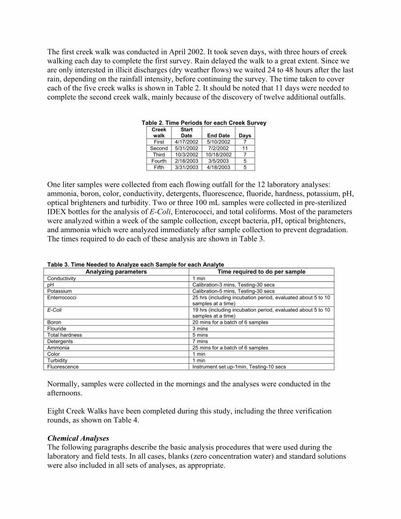
The first creek walk was conducted in April 2002. It took seven days, with three hours of creek walking each day to complete the first survey. Rain delayed the walk to a great extent. Since we are only interested in illicit discharges (dry weather flows) we waited 24 to 48 hours after the last rain, depending on the rainfall intensity, before continuing the survey. The time taken to cover each of the five creek walks is shown in Table 2. It should be noted that 11 days were needed to complete the second creek walk, mainly because of the discovery of twelve additional outfalls.

Table 2. Time Periods for each Creek Survey Creek walk

Start Date End Date Days

First 4/17/2002 5/10/2002 7 Second 5/31/2002 7/2/2002 11

Third 10/3/2002 10/18/2002 7 Fourth 2/18/2003 3/5/2003 5 Fifth 3/31/2003 4/18/2003 5

One liter samples were collected from each flowing outfall for the 12 laboratory analyses: ammonia, boron, color, conductivity, detergents, fluorescence, fluoride, hardness, potassium, pH, optical brighteners and turbidity. Two or three 100 mL samples were collected in pre-sterilized IDEX bottles for the analysis of E-Coli, Enterococci, and total coliforms. Most of the parameters were analyzed within a week of the sample collection, except bacteria, pH, optical brighteners, and ammonia which were analyzed immediately after sample collection to prevent degradation. The times required to do each of these analysis are shown in Table 3.

Table 3. Time Needed to Analyze each Sample for each Analyte Analyzing parameters Time required to do per sample

Conductivity 1 min pH Calibration-3 mins, Testing-30 secs Potassium Calibration-5 mins, Testing-30 secs Enterrococci 25 hrs (including incubation period, evaluated about 5 to 10

samples at a time) E-Coli 19 hrs (including incubation period, evaluated about 5 to 10

samples at a time) Boron 20 mins for a batch of 6 samples Flouride 3 mins Total hardness 5 mins Detergents 7 mins Ammonia 25 mins for a batch of 6 samples Color 1 min Turbidity 1 min Fluorescence Instrument set up-1min, Testing-10 secs

Normally, samples were collected in the mornings and the analyses were conducted in the afternoons.

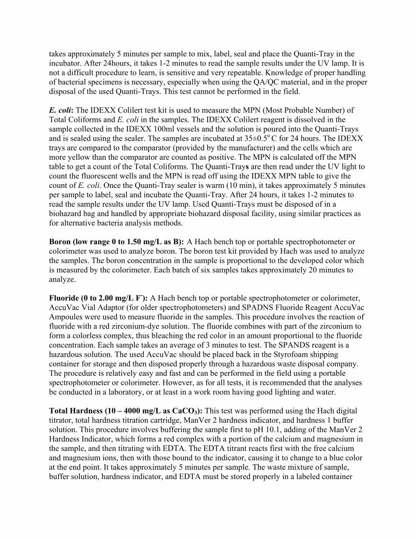
Eight Creek Walks have been completed during this study, including the three verification rounds, as shown on Table 4.

Chemical Analyses The following paragraphs describe the basic analysis procedures that were used during the laboratory and field tests. In all cases, blanks (zero concentration water) and standard solutions were also included in all sets of analyses, as appropriate.

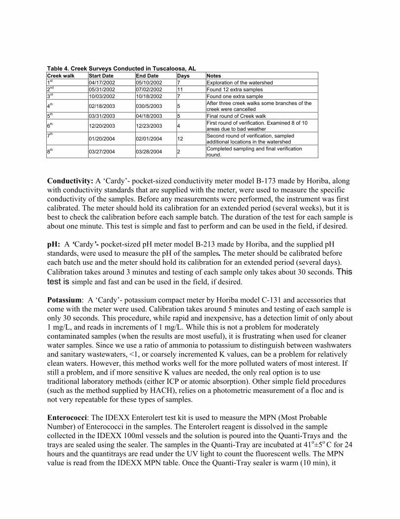
Table 4. Creek Surveys Conducted in Tuscaloosa, AL Creek walk Start Date End Date Days Notes 1st 04/17/2002 05/10/2002 7 Exploration of the watershed 2nd 05/31/2002 07/02/2002 11 Found 12 extra samples 3rd 10/03/2002 10/18/2002 7 Found one extra sample

4th 02/18/2003 030/5/2003 5 After three creek walks some branches of the creek were cancelled

5th 03/31/2003 04/18/2003 5 Final round of Creek walk

6th 12/20/2003 12/23/2003 4 First round of verification. Examined 8 of 10 areas due to bad weather

7th

01/20/2004 02/01/2004 12 Second round of verification, sampled additional locations in the watershed

8th 03/27/2004 03/28/2004 2 Completed sampling and final verification round.

Conductivity: A ‘Cardy’- pocket-sized conductivity meter model B-173 made by Horiba, along with conductivity standards that are supplied with the meter, were used to measure the specific conductivity of the samples. Before any measurements were performed, the instrument was first calibrated. The meter should hold its calibration for an extended period (several weeks), but it is best to check the calibration before each sample batch. The duration of the test for each sample is about one minute. This test is simple and fast to perform and can be used in the field, if desired.

pH: A ‘Cardy’- pocket-sized pH meter model B-213 made by Horiba, and the supplied pH standards, were used to measure the pH of the samples. The meter should be calibrated before each batch use and the meter should hold its calibration for an extended period (several days). Calibration takes around 3 minutes and testing of each sample only takes about 30 seconds. This test is simple and fast and can be used in the field, if desired.

Potassium: A ‘Cardy’- potassium compact meter by Horiba model C-131 and accessories that come with the meter were used. Calibration takes around 5 minutes and testing of each sample is only 30 seconds. This procedure, while rapid and inexpensive, has a detection limit of only about 1 mg/L, and reads in increments of 1 mg/L. While this is not a problem for moderately contaminated samples (when the results are most useful), it is frustrating when used for cleaner water samples. Since we use a ratio of ammonia to potassium to distinguish between washwaters and sanitary wastewaters, <1, or coarsely incremented K values, can be a problem for relatively clean waters. However, this method works well for the more polluted waters of most interest. If still a problem, and if more sensitive K values are needed, the only real option is to use traditional laboratory methods (either ICP or atomic absorption). Other simple field procedures (such as the method supplied by HACH), relies on a photometric measurement of a floc and is not very repeatable for these types of samples.

Enterococci: The IDEXX Enterolert test kit is used to measure the MPN (Most Probable Number) of Enterococci in the samples. The Enterolert reagent is dissolved in the sample collected in the IDEXX 100ml vessels and the solution is poured into the Quanti-Trays and the trays are sealed using the sealer. The samples in the Quanti-Tray are incubated at 41o±5o C for 24 hours and the quantitrays are read under the UV light to count the fluorescent wells. The MPN value is read from the IDEXX MPN table. Once the Quanti-Tray sealer is warm (10 min), it

takes approximately 5 minutes per sample to mix, label, seal and place the Quanti-Tray in the incubator. After 24hours, it takes 1-2 minutes to read the sample results under the UV lamp. It is not a difficult procedure to learn, is sensitive and very repeatable. Knowledge of proper handling of bacterial specimens is necessary, especially when using the QA/QC material, and in the proper disposal of the used Quanti-Trays. This test cannot be performed in the field.

E. coli: The IDEXX Colilert test kit is used to measure the MPN (Most Probable Number) of Total Coliforms and E. coli in the samples. The IDEXX Colilert reagent is dissolved in the sample collected in the IDEXX 100ml vessels and the solution is poured into the Quanti-Trays and is sealed using the sealer. The samples are incubated at 35±0.5o C for 24 hours. The IDEXX trays are compared to the comparator (provided by the manufacturer) and the cells which are more yellow than the comparator are counted as positive. The MPN is calculated off the MPN table to get a count of the Total Coliforms. The Quanti-Trays are then read under the UV light to count the fluorescent wells and the MPN is read off using the IDEXX MPN table to give the count of E. coli. Once the Quanti-Tray sealer is warm (10 min), it takes approximately 5 minutes per sample to label, seal and incubate the Quanti-Tray. After 24 hours, it takes 1-2 minutes to read the sample results under the UV lamp. Used Quanti-Trays must be disposed of in a biohazard bag and handled by appropriate biohazard disposal facility, using similar practices as for alternative bacteria analysis methods.

Boron (low range 0 to 1.50 mg/L as B): A Hach bench top or portable spectrophotometer or colorimeter was used to analyze boron. The boron test kit provided by Hach was used to analyze the samples. The boron concentration in the sample is proportional to the developed color which is measured by the colorimeter. Each batch of six samples takes approximately 20 minutes to analyze.

Fluoride (0 to 2.00 mg/L F-): A Hach bench top or portable spectrophotometer or colorimeter, AccuVac Vial Adaptor (for older spectrophotometers) and SPADNS Fluoride Reagent AccuVac Ampoules were used to measure fluoride in the samples. This procedure involves the reaction of fluoride with a red zirconium-dye solution. The fluoride combines with part of the zirconium to form a colorless complex, thus bleaching the red color in an amount proportional to the fluoride concentration. Each sample takes an average of 3 minutes to test. The SPANDS reagent is a hazardous solution. The used AccuVac should be placed back in the Styrofoam shipping container for storage and then disposed properly through a hazardous waste disposal company. The procedure is relatively easy and fast and can be performed in the field using a portable spectrophotometer or colorimeter. However, as for all tests, it is recommended that the analyses be conducted in a laboratory, or at least in a work room having good lighting and water.

Total Hardness (10 – 4000 mg/L as CaCO3): This test was performed using the Hach digital titrator, total hardness titration cartridge, ManVer 2 hardness indicator, and hardness 1 buffer solution. This procedure involves buffering the sample first to pH 10.1, adding of the ManVer 2 Hardness Indicator, which forms a red complex with a portion of the calcium and magnesium in the sample, and then titrating with EDTA. The EDTA titrant reacts first with the free calcium and magnesium ions, then with those bound to the indicator, causing it to change to a blue color at the end point. It takes approximately 5 minutes per sample. The waste mixture of sample, buffer solution, hardness indicator, and EDTA must be stored properly in a labeled container

until disposal by a hazardous waste disposal facility. It is not recommended to perform this procedure in the field.

Detergents (0-3ppm): Detergents were analyzed using the Detergents (anionic surfactants) kit from CHEMetrics. The following procedure comes with the Detergent kit. The Detergents CHEMets® test employs the methylene blue extraction method. Anionic detergents react with methylene blue to form a blue complex that is extracted into an immiscible organic solvent. The intensity of the blue color is directly related to the concentration of “methylene blue active substances (MBAS)” in the sample. Anionic detergents are one of the most prominent methylene blue active substances. Test results are expressed in mg/L linear alkylbenzene sulfonate. It takes approximately 7 minutes per sample. This method uses a small amount of chloroform and extra precautions are therefore necessary during the test and when disposing of this hazardous material.

Ammonia (0 to 0.50 mg/L NH3-N): A Hach bench top, or portable spectrophotometer or colorimeter, ammonia nitrogen reagent set for 25-mL samples, and ammonia nitrogen standard solution were used for this test. In this method, ammonia compounds combine with chlorine to form monochloramine. Monochloramine reacts with salicylate to form 5-aminosalicylate. The 5­aminosalicylate is oxidized in the presence of sodium nitroprusside catalyst to form a blue-colored compound. The blue color is masked by the yellow color from the excess reagent present to give a final green-colored solution. Because of the duration of this test, it is best to run samples in batches of about 6. From start to finish, each batch of 6 samples takes about 25 minutes, including the time taken to clean the sample cells and reset the instrument between each batch. According to good laboratory practice, the contents of each sample cell, after the analysis, should be poured into another properly-labeled container for proper disposal. This procedure is time-consuming and should be performed indoors.

Color (0 – 100 APHA Platinum Cobalt Units): Color is measured using a Hach color test kit (Model CO-1), which measures color using a color disc for comparison. The sample is compared to a clean water tube and using the comparator, a match to the color of the sample is made. The readings on the comparator disc give the measurement of color in APHA Platinum Cobalt Units. It takes about one minute to read a sample. This procedure is easy and fast and can be performed outside of the laboratory, if desired.

Turbidity (NTU): A bench-top or portable turbidimeter is used to analyze turbidity. However, the portable turbidimeter has a much narrower analytical range compared to the laboratory instrument. The range of readings in NTU will depend upon the instrument. The instrument must be calibrated using the secondary standards supplied with the instrument. These secondary standards (very stable) need to be periodically checked against primary turbidity standards (which are unstable after dilution). Samples are normally stored under refrigeration prior to analysis. Before analyzing for turbidity, the samples must first be brought back to room temperature to prevent the formation of frost on the outside of the glass sample cells used in the turbidity measurement. The sample cell containing the sample is placed into the turbidimeter and the reading is noted. It takes approximately one minute to take a sample reading. It is a relatively simple test and may be performed outside the laboratory using a portable turbidimeter.

Fluorescence: Fluorescence is the property of the whiteners in detergents that cause treated fabrics to fluoresce in the presence of ultraviolet rays, giving laundered materials an impression of extra cleanliness. These are also referred to as bluing, brighteners or optical brighteners and have been an important ingredient of most laundry detergents for many years. The effectiveness of the brighteners varies by the concentration of the detergents in the wash water. The detection of optical brighteners has been used as an indicator for the presence of laundry wastewater, and municipal sewage, in urban waters. One method of quantifying fluorescence in the laboratory is by using a fluorometer calibrated for detergents. In our tests, we used the GFL-1 Portable Field fluorometer. This is a very sensitive instrument, but expensive. However, the analytical time needed to measure sample fluorescence is very short.

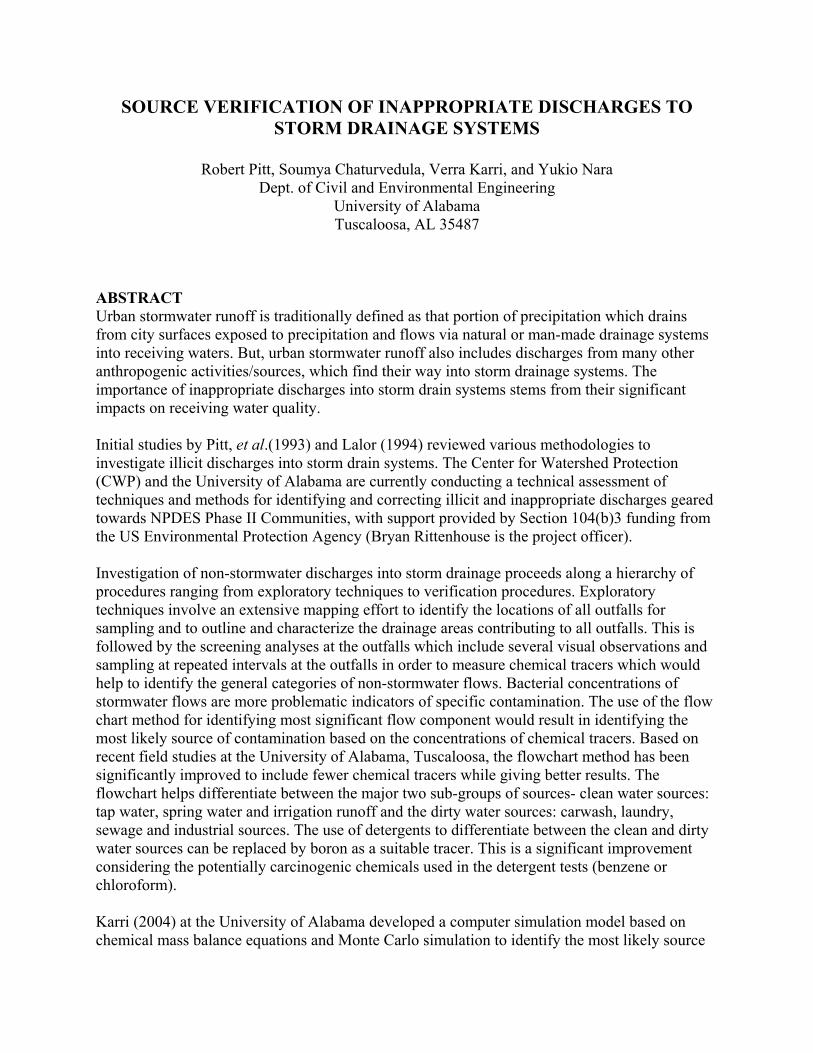
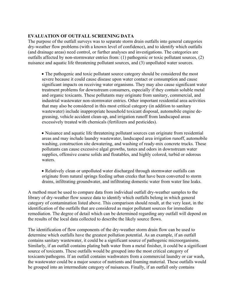
Optical Brighteners(mg/L as Tide): A test for optical brighteners, developed by Don Waye and used in his research in Northern Virginia, was also examined as a possible substitute for the detergents or fluorescence test. In this test, cotton pads enclosed in a steel grid covered with a plastic mesh are placed in the outfalls for at least 24 hours and are then brought back to the laboratory and dried. The dried pads are then viewed under the UV lamp to check for fluorescence. Standards of these cotton pads with pure samples of different concentrations of Tide detergent were prepared and the cotton pads from the outfalls were compared to these standards to estimate the concentration of detergent in the flows (Figure 1). The fluorescence of these pads was affected by deposits of silt and dirt onto these cotton pads (which was actually helpful to indicate irregular flows). Unfortunately, the method was found to be very insensitive, requiring almost 50 mg/L of Tide detergent (similar to full strength wash water) to be present before a positive indication could be selected. However, if a clean pad was placed in an outfall, sheltered by the pipe, and it was later found to be fouled, that is a good indicator of the presence of intermittent dry weather flows.

Figure 1. Standard Tide Optical Brightener Pads

EVALUATION OF OUTFALL SCREENING DATA The purpose of the outfall surveys was to separate storm drain outfalls into general categories dry-weather flow problems (with a known level of confidence), and to identify which outfalls (and drainage areas) need control, or further analyses and investigations. The categories are outfalls affected by non-stormwater entries from: (1) pathogenic or toxic pollutant sources, (2) nuisance and aquatic life threatening pollutant sources, and (3) unpolluted water sources.

• The pathogenic and toxic pollutant source category should be considered the most severe because it could cause disease upon water contact or consumption and cause significant impacts on receiving water organisms. They may also cause significant water treatment problems for downstream consumers, especially if they contain soluble metal and organic toxicants. These pollutants may originate from sanitary, commercial, and industrial wastewater non-stormwater entries. Other important residential area activities that may also be considered in this most critical category (in addition to sanitary wastewater) include inappropriate household toxicant disposal, automobile engine de-greasing, vehicle accident clean-up, and irrigation runoff from landscaped areas excessively treated with chemicals (fertilizers and pesticides).

• Nuisance and aquatic life threatening pollutant sources can originate from residential areas and may include laundry wastewater, landscaped area irrigation runoff, automobile washing, construction site dewatering, and washing of ready-mix concrete trucks. These pollutants can cause excessive algal growths, tastes and odors in downstream water supplies, offensive coarse solids and floatables, and highly colored, turbid or odorous waters.

• Relatively clean or unpolluted water discharged through stormwater outfalls can originate from natural springs feeding urban creeks that have been converted to storm drains, infiltrating groundwater, and infiltrating domestic water from water line leaks.

A method must be used to compare data from individual outfall dry-weather samples to the library of dry-weather flow source data to identify which outfalls belong in which general category of contamination listed above. This comparison should result, at the very least, in the identification of the outfalls that are considered as major pollutant sources for immediate remediation. The degree of detail which can be determined regarding any outfall will depend on the results of the local data collected to describe the likely source flows.

The identification of flow components of the dry-weather storm drain flow can be used to determine which outfalls have the greatest pollution potential. As an example, if an outfall contains sanitary wastewater, it could be a significant source of pathogenic microorganisms. Similarly, if an outfall contains plating bath water from a metal finisher, it could be a significant source of toxicants. These outfalls would be grouped into the most critical category of toxicants/pathogens. If an outfall contains washwaters from a commercial laundry or car wash, the wastewater could be a major source of nutrients and foaming material. These outfalls would be grouped into an intermediate category of nuisances. Finally, if an outfall only contains

unpolluted groundwater or water from leaky potable water mains, the water would be non­polluting and the outfall would be grouped into the last category of clean water sources.

Indicators of Contamination Indicators of contamination (negative indicators) are clearly apparent visual or physical parameters indicating obvious problems and are readily observable at the outfall during field screening activities. These observations are very important during the field survey because they are the simplest method of identifying grossly contaminated dry-weather outfall flows. The direct examination of outfall characteristics for unusual conditions of flow, odor, color, turbidity, floatables, deposits/stains, vegetation conditions, and damage to drainage structures is therefore an important part of these investigations. The following list summarizes these indicators, along with narratives of the descriptors to be selected in the field.

Odor - Most strong odors, especially sewage, gasoline, oils, and solvents, are likely associated with the most hazardous discharges. Typical obvious odors include: gasoline, oil, sanitary wastewater, industrial chemicals, decomposing organic wastes, etc.

sewage: smell associated with stale sanitary wastewater, especially in pools near outfall. sulfur (“rotten eggs”): industries that discharge sulfide compounds or organics (meat

packers, canneries, dairies, etc.). oil and gas: petroleum refineries or many facilities associated with vehicle maintenance

or petroleum product storage. rancid-sour: food preparation facilities (restaurants, hotels, etc.).

Color - Important indicator of inappropriate industrial sources. Industrial dry-weather discharges may be of any color, but dark colors, such as brown, gray, or black, are most common.

yellow: chemical plants, textile and tanning plants. brown: meat packers, printing plants, metal works, stone and concrete, fertilizers,

and petroleum refining facilities. green: chemical plants, textile facilities. red: meat packers. gray: dairies.

Turbidity - Often affected by the degree of gross contamination. Dry-weather industrial flows with moderate turbidity can be cloudy, while highly turbid flows can be opaque. High turbidity is often a characteristic of undiluted dry-weather industrial discharges.

cloudy: sanitary wastewater, concrete or stone operations, fertilizer facilities, automotive dealers.

opaque: food processors, lumber mills, metal operations, pigment plants.

Floatable Matter - A contaminated flow may contain floating solids or liquids directly related to industrial or sanitary wastewater pollution. Floatables of industrial origin may include animal fats, spoiled food, oils, solvents, sawdust, foams, packing materials, or fuel. oil sheen: petroleum refineries or storage facilities and vehicle service facilities.

sewage: sanitary wastewater.

Deposits and Stains - Refer to any type of coating near the outfall and are usually of a dark color. Deposits and stains often will contain fragments of floatable substances. These situations are illustrated by the grayish-black deposits that contain fragments of animal flesh and hair which often are produced by leather tanneries, or the white crystalline powder which commonly coats outfalls due to nitrogenous fertilizer wastes. sediment: construction site erosion.

oily: petroleum refineries or storage facilities and vehicle service facilities.

Vegetation - Vegetation surrounding an outfall may show the effects of industrial pollutants. Decaying organic materials coming from various food product wastes would cause an increase in plant life, while the discharge of chemical dyes and inorganic pigments from textile mills could noticeably decrease vegetation. It is important not to confuse the adverse effects of high stormwater flows on vegetation with highly toxic dry-weather intermittent flows. excessive growth: food product facilities. inhibited growth: high stormwater flows, beverage facilities, printing plants, metal

product facilities, drug manufacturing, petroleum facilities, vehicle service facilities and automobile dealers.

Damage to Outfall Structures - Another readily visible indication industrial contamination. Cracking, deterioration, and spalling of concrete or peeling of surface paint, occurring at an outfall are usually caused by severely contaminated discharges, usually of industrial origin. These contaminants are usually very acidic or basic in nature. Primary metal industries have a strong potential for causing outfall structural damage because their batch dumps are highly acidic. Poor construction, hydraulic scour, and old age may also adversely affect the condition of the outfall structure. concrete cracking: industrial flows concrete spalling: industrial flows peeling paint: industrial flows metal corrosion: industrial flows

This method does not allow quantifiable estimates of the flow components and it will very likely result in many incorrect negative determinations (missing outfalls that have important levels of contamination). These simple characteristics are most useful for identifying gross contamination. Only the most significant outfalls and drainage areas would therefore be recognized from this method. The other methods, requiring chemical determinations, can be used to quantify the flow contributions and to identify the less obviously contaminated outfalls. In all cases, water samples should be collected for later laboratory analyses by the field team conducting the field surveys to supplement the initial impressions of these gross indicators.

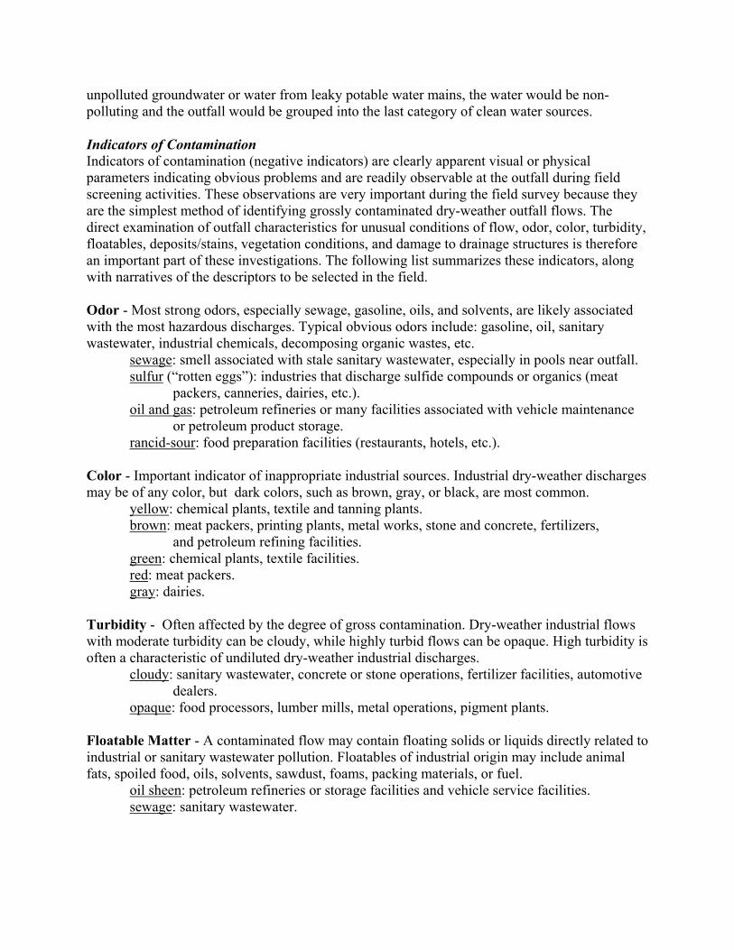
Indications of intermittent flows (especially stains or damage to the structure of the outfall) could indicate serious illegal toxic pollutant entries into the storm drainage system that will be very difficult to detect and correct. Highly irregular dry-weather outfall flow rates or chemical characteristics could indicate industrial or commercial inappropriate entries into the storm drain system. Table 5 summarizes the physical characteristics of source flows as observed by Pitt, et al. (1993) in Birmingham, AL.

Table 5. Summary of Physical Characteristics of Source Samples (number of negative responses/number of samples evaluated) (Pitt, et al. 1993)

Source Color Odor Turbidity Floatables/Sheens Sediments Spring Water Shallow Ground Tap Water Landscape Irrigation Sanitary Sewage Septic Tank Discharge Carwash Wastewater Laundry Wastewater Radiator Wastes Plating Wastewaters

0/10 6/10 0\10

36/36 13\13 10\10 10\10 10\10 10\10 10\10

0\10 0\10 0\10 0\10 36\36 8\13 3\10 5\10

10\10 5\10

0\10 0\10 0\10 2\10 36\36 0\13 10\10 10\10 8\10 2\10

0\10 0\10 0\10 2\10 NA

0\13 3\10 3\10

10\10 0\10

0\10 0\10 0\10 0\10 NA

0\13 6\10 0\10 2\10 10\10

NA: Data not available

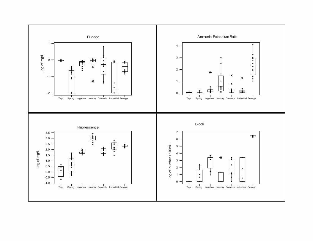
Development of flowchart methodology The flowchart methodology was initially described by Pitt, et al. (1993). Following a hierarchy of prescribed limits of tracers, the flowchart makes it possible to identify the most probable source of contamination. The following flow chart describes an analysis strategy which can be used to identify the major component of dry-weather flow samples in residential and commercial areas. This method does not attempt to distinguish among all potential sources of dry-weather flow identified earlier, but rather the following four major groups of flow are identified: (1) tap waters (tap water, irrigation water and rinse water), (2) natural waters (spring water and shallow ground water), (3) sanitary wastewaters (sanitary sewage and septic tank discharge), and (4) wash waters (commercial laundry waters, commercial car wash waters, radiator flushing wastes, and plating bath wastewaters). The use of this method would not only allow outfall flows to be categorized as contaminated or uncontaminated, but would allow outfalls carrying sanitary wastewaters to be identified. These outfalls could then receive highest priority for further investigation leading to source control.

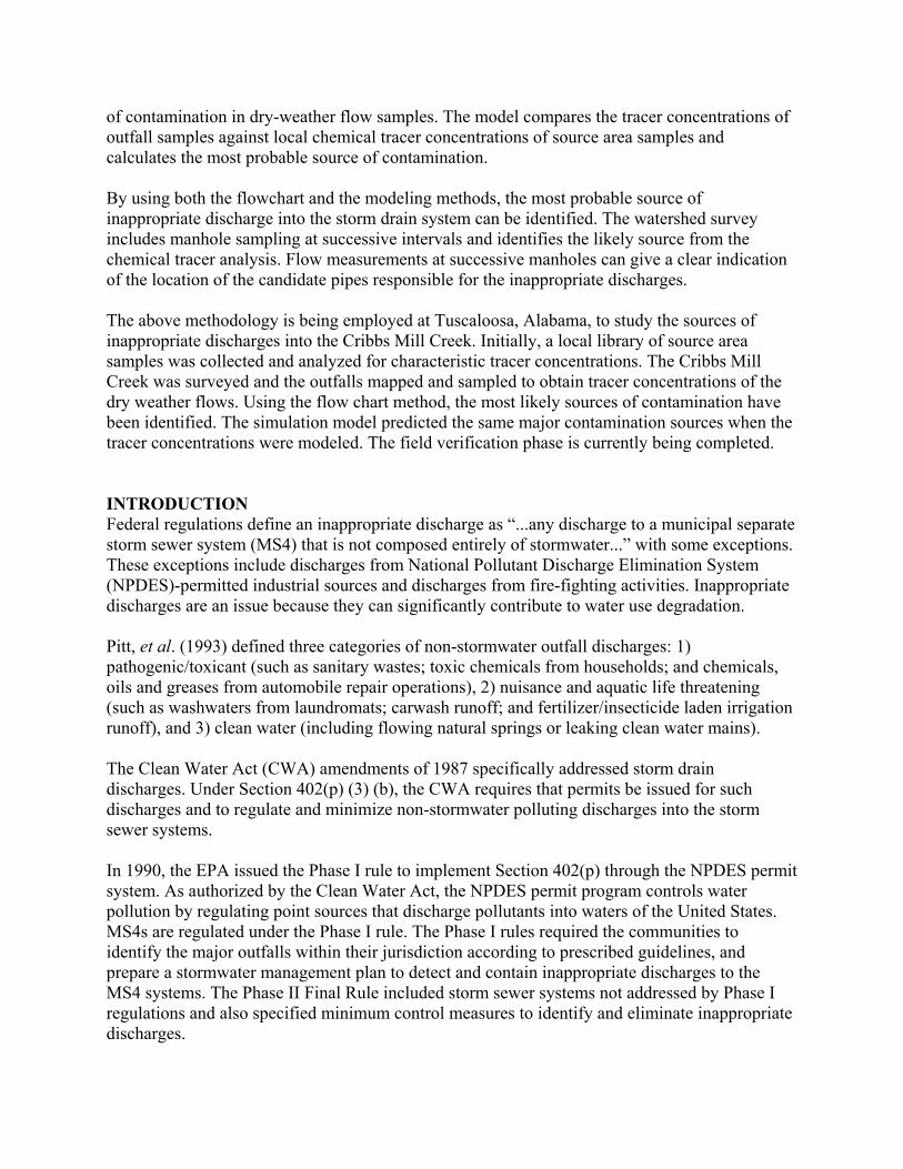
The original flowchart developed by Pitt, et al. (1993) was modified during the current project to reflect the current analytical methods and some changes in the tracers. The library tracer concentrations were used as a basis to find tracers which show unique values for different sources of contamination, as shown on the attached grouped bar and whisker plots. A hierarchy of tracer concentrations was then derived, which would ultimately pin-point the source of contamination.

Our research found that boron and detergents can be used to distinguish the clean waters from the dirty waters. Within the dirty waters the ammonia/potassium ratio can be used to distinguish between the sanitary wastewaters and the washwaters. Among the twelve laundry samples taken, two samples showed an ammonia/potassium ratio value of greater than 1, but all of the sanitary wastewaters showed an ammonia/potassium ratio greater than 1. From other analyses of sewage dilution, this has been found to be a robust tracer to differentiate between the dirty waters. Fluoride concentrations can be used to distinguish between the clean waters. Tap water and irrigation water (since it originates from tap water) can be differentiated from spring water by using fluoride as a tracer as fluoride is added to tap water in concentrations required by local regulations. Spring water, on the other hand will not have anthropogenic concentrations of

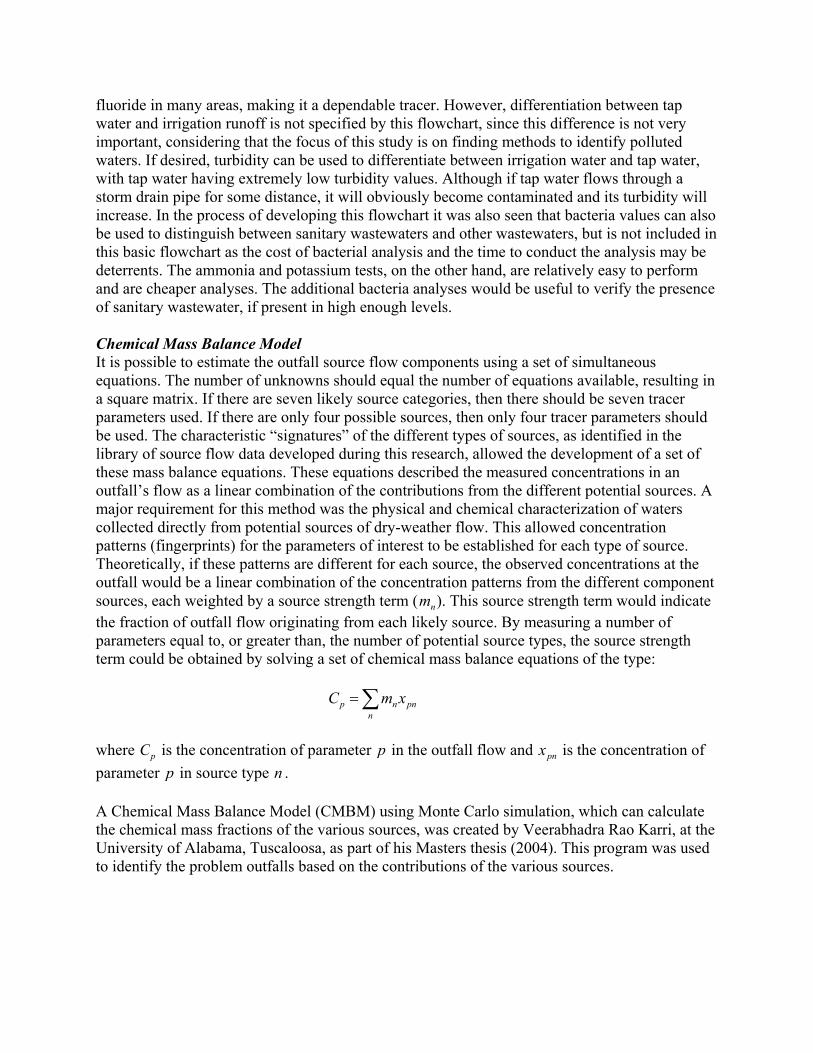
fluoride in many areas, making it a dependable tracer. However, differentiation between tap water and irrigation runoff is not specified by this flowchart, since this difference is not very important, considering that the focus of this study is on finding methods to identify polluted waters. If desired, turbidity can be used to differentiate between irrigation water and tap water, with tap water having extremely low turbidity values. Although if tap water flows through a storm drain pipe for some distance, it will obviously become contaminated and its turbidity will increase. In the process of developing this flowchart it was also seen that bacteria values can also be used to distinguish between sanitary wastewaters and other wastewaters, but is not included in this basic flowchart as the cost of bacterial analysis and the time to conduct the analysis may be deterrents. The ammonia and potassium tests, on the other hand, are relatively easy to perform and are cheaper analyses. The additional bacteria analyses would be useful to verify the presence of sanitary wastewater, if present in high enough levels.

Chemical Mass Balance Model It is possible to estimate the outfall source flow components using a set of simultaneous equations. The number of unknowns should equal the number of equations available, resulting in a square matrix. If there are seven likely source categories, then there should be seven tracer parameters used. If there are only four possible sources, then only four tracer parameters should be used. The characteristic “signatures” of the different types of sources, as identified in the library of source flow data developed during this research, allowed the development of a set of these mass balance equations. These equations described the measured concentrations in an outfall’s flow as a linear combination of the contributions from the different potential sources. A major requirement for this method was the physical and chemical characterization of waters collected directly from potential sources of dry-weather flow. This allowed concentration patterns (fingerprints) for the parameters of interest to be established for each type of source. Theoretically, if these patterns are different for each source, the observed concentrations at the outfall would be a linear combination of the concentration patterns from the different component sources, each weighted by a source strength term (mn ). This source strength term would indicate the fraction of outfall flow originating from each likely source. By measuring a number of parameters equal to, or greater than, the number of potential source types, the source strength term could be obtained by solving a set of chemical mass balance equations of the type:

Cp =∑mn xpn n

where Cp is the concentration of parameter p in the outfall flow and xpn is the concentration of parameter p in source type n .

A Chemical Mass Balance Model (CMBM) using Monte Carlo simulation, which can calculate the chemical mass fractions of the various sources, was created by Veerabhadra Rao Karri, at the University of Alabama, Tuscaloosa, as part of his Masters thesis (2004). This program was used to identify the problem outfalls based on the contributions of the various sources.

Sewage Industrial Carwash Laundry Irrigation Spring Tap

1

0

-1

-2

Log

of m

g/L

Fluoride

Tap Spring Irrigation Laundry Carwash Industrial Sewage

-1.0

-0.5

0.0

0.5

1.0

1.5

2.0

2.5

3.0

3.5

Log

of m

g/L

Fluorescence

Tap Spring Irrigation Laundry Carwash Industrial Sewage

0

1

2

3

4

Ammonia-Potassium Ratio

Sewage Industrial Carwash Laundry Irrigation Spring Tap

7

6

5

4

3

2

1

0

Log

of n

umbe

r / 1

00m

L

E-coli

The library tracer data was evaluated for normal, or log-normal distribution fits using the Anderson Darling test. The model uses the input values of the sources and tracers to be evaluated from the existing library data file, according to selections of the model user (the number of tracers used must equal the number of possible sources being examined). The mass fractions of the sources contributing to the outfall are then calculated using matrix algebra. The matrix algebra method used in this model involves solving a set of simultaneous chemical mass balance equations for the mass fraction values at the outfall. The model compares the tracer concentrations of outfall samples against local chemical tracer concentrations of pure source samples and from the ensuing mass balance equations returns the most probable source of contamination.

Since there is variability within the library data for each tracer, these equations have to be solved using a number of values of concentrations within the appropriate data distributions (log or log­normal) of these concentration values. Monte Carlo simulation is used to accomplish this task. Once the probability of correctness in the prediction of the source water is quantified, one can make a decision as to the most likely inappropriate source(s) contributing to the outfall discharge. If such a quantitative assessment of uncertainty was not conducted, insufficient water quality improvements and misallocation of other resources could result.

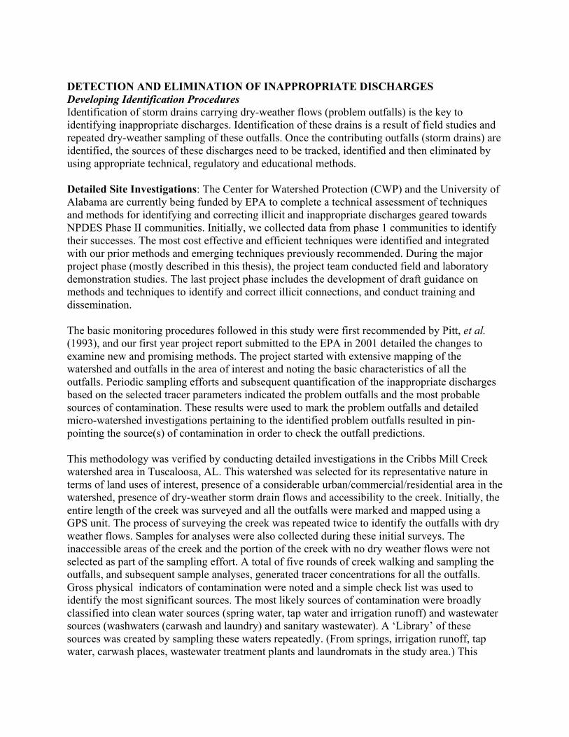
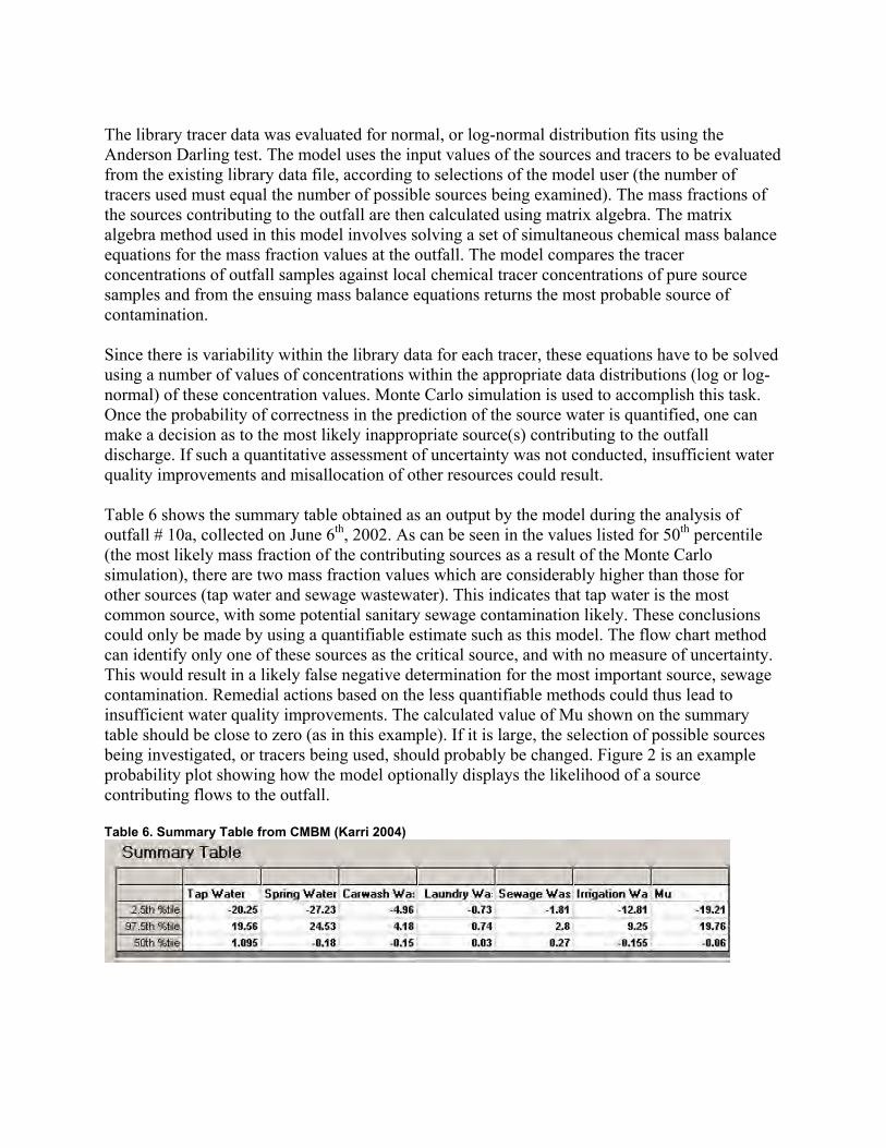
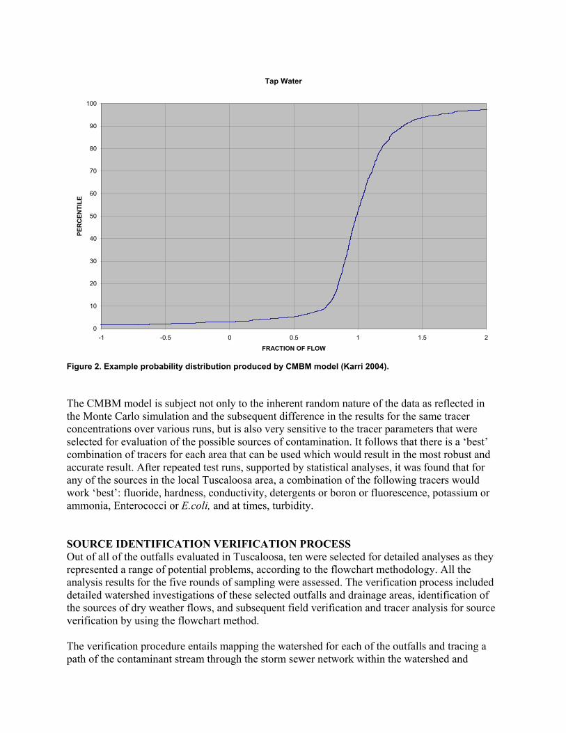
Table 6 shows the summary table obtained as an output by the model during the analysis of outfall # 10a, collected on June 6th, 2002. As can be seen in the values listed for 50th percentile (the most likely mass fraction of the contributing sources as a result of the Monte Carlo simulation), there are two mass fraction values which are considerably higher than those for other sources (tap water and sewage wastewater). This indicates that tap water is the most common source, with some potential sanitary sewage contamination likely. These conclusions could only be made by using a quantifiable estimate such as this model. The flow chart method can identify only one of these sources as the critical source, and with no measure of uncertainty. This would result in a likely false negative determination for the most important source, sewage contamination. Remedial actions based on the less quantifiable methods could thus lead to insufficient water quality improvements. The calculated value of Mu shown on the summary table should be close to zero (as in this example). If it is large, the selection of possible sources being investigated, or tracers being used, should probably be changed. Figure 2 is an example probability plot showing how the model optionally displays the likelihood of a source contributing flows to the outfall.

Table 6. Summary Table from CMBM (Karri 2004)

Tap Water

0

10

20

30

40

50

60

70

80

90

100

PER

CEN

TILE

-1 -0.5 0 0.5 1 1.5

FRACTION OF FLOW

Figure 2. Example probability distribution produced by CMBM model (Karri 2004).

The CMBM model is subject not only to the inherent random nature of the data as reflected in the Monte Carlo simulation and the subsequent difference in the results for the same tracer concentrations over various runs, but is also very sensitive to the tracer parameters that were selected for evaluation of the possible sources of contamination. It follows that there is a ‘best’ combination of tracers for each area that can be used which would result in the most robust and accurate result. After repeated test runs, supported by statistical analyses, it was found that for any of the sources in the local Tuscaloosa area, a combination of the following tracers would work ‘best’: fluoride, hardness, conductivity, detergents or boron or fluorescence, potassium or ammonia, Enterococci or E.coli, and at times, turbidity.

SOURCE IDENTIFICATION VERIFICATION PROCESS Out of all of the outfalls evaluated in Tuscaloosa, ten were selected for detailed analyses as they represented a range of potential problems, according to the flowchart methodology. All the analysis results for the five rounds of sampling were assessed. The verification process included detailed watershed investigations of these selected outfalls and drainage areas, identification of the sources of dry weather flows, and subsequent field verification and tracer analysis for source verification by using the flowchart method.

The verification procedure entails mapping the watershed for each of the outfalls and tracing a path of the contaminant stream through the storm sewer network within the watershed and

2

ultimately pin-pointing the source. Typically, the verification process included taking samples at the designated problem outfalls, investigating further on into the watershed by finding the associated storm drain network and taking samples at each manhole as we went upstream into the watershed, until a point is reached where there was no sign of dry weather flows. The source was then determined to be near the most upstream manhole in the watershed where dry weather flows was last noticed.

In the case of continuous dry-weather flows in the drainage system, the flows are sampled from the outfall to the boundary of the watershed or to the source of flow. The drainage system is roughly divided into thirds, and samples are obtained at these divisions. Differences in the tracer concentrations, or flows, between these sampling locations can be used to identify the area where the flows originate in the drainage system. Examining the residences and commercial establishments in the identified area where the flows or inappropriate discharges occur, including possibly investigating floor drains or discharges originating from these locations may be necessary. This information coupled with the predicted source of flows from the source characterization studies (the flow chart and/or the Monte Carlo mixing model) can narrow the likely source down to a few potential candidates. The following discussion is an example of the evaluation for one of the selected outfalls.

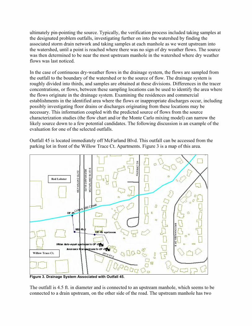
Outfall 45 is located immediately off McFarland Blvd. This outfall can be accessed from the parking lot in front of the Willow Trace Ct. Apartments. Figure 3 is a map of this area.

Red Lobster

Willow Trace Ct.

Figure 3. Drainage System Associated with Outfall 45.

The outfall is 4.5 ft. in diameter and is connected to an upstream manhole, which seems to be connected to a drain upstream, on the other side of the road. The upstream manhole has two

inflow pipes, one from the stream on the other side of McFarland and one coming in from upstream, along the road. The pipe coming from across McFarland was always found to be flowing, but the pipe coming in from along the road was showing a trickling flow only in the last verification sampling period. The flow coming into this manhole seems to be originating from behind a local insurance office. There is about a 9” pipe found discharging into this stream. This pipe could be the source of the washwater predicted at the outfall. No pipes were found originating from the Midas automobile repair shop. Table 7 shows the results from the creek surveys and source investigation tests for this outfall.

Table 7. Creek Survey and Source Investigation Results for Outfall 45

Sample ID Date of collection

Problem indicated by physical observations

Detergents contamination (yes if ≥ 0.25 mg/l or Yes if boron ≥ 0.35)

Flow chart method, most likely source

45

5/8/2002 No Yes Washwater source

6/24/2002 No Yes Washwater source

10/18/2002 No No Tap water source

3/5/2003 No Yes Washwater source

No Yes Washwater source

12/22/2003 No Yes Washwater source

1/30/2004 No Yes Washwater source

3/28/2004 Yes No Natural water source

OF 45 upstream 1/30/2004 No No Natural water source

OF 45 upstream 3/28/2004 No No Tap/irrigation water source

MH 45.1 2/1/2004 No Yes Washwater source

MH 45.1 3/28/2004 No Yes Washwater source

The results show that there is potential washwater contamination at this outfall. In all cases, except the last two, the detergent concentrations were high, but the last two showed high boron concentrations. In the third round of verification investigations, frothing could be seen at the outfall. It was also observed that while the connecting manhole likely had a washwater source, neither the outfall nor the upstream stream indicated detergent contamination. At the outfall, this could be an effect of the dilution with natural spring water. The upstream area showed a moderate boron concentration of 0.27 mg/L, thus indicating irrigation/tap water but not washwater. Hence, it seems possible that water flowing into the manhole from the pipe along the road could be carrying washwater. However, it was not clear where this pipe was originating.

None of the manholes upstream to this manhole had pipes pointing in the direction of this manhole.

The outfalls were considered to be contaminated if the source waters predicted by the model were other than irrigation, tap, or spring water. Table 8 shows the comparison of the mass balance model predictions with the other methods for all 10 of the selected outfalls. The physical observation method relies on obvious indicators such as highly colored or turbid water, gross floatables present near the outfall, etc. The detergents method considers an outfall to be contaminated if the concentration of detergents is ≥ 0.25 mg/L. The flow chart method considers an outfall to be contaminated if the likely source predicted by the flowchart method (using a number of chemical tracers, such as detergents, fluoride, boron, potassium, ammonia, and bacteria) is other than irrigation, tap, or spring water. These comparisons show that the predictions with respect to contamination are consistent with the other methods of source identification. These ten outfalls are undergoing additional watershed investigations, as noted above, to further verify the model results. Initial results indicate that the mass balance predictions are accurate indicators of the source flows. Karri (2004) also presents complete analyses for each outfall for each of the five complete creek surveys. During these surveys, at least 39 outfalls were sampled five times. All of the analysis methods were applied to these outfalls for comparison.

CONCLUSIONS Tables 9 through 11 summarize the verification evaluations conducted earlier by Pitt, et al. (1993) in Birmingham, AL, using several different evaluation methods. The use of negative indicators alone resulted in several false negatives and false positives, while the flow chart method correctly identified the major discharge and the earlier version of the chemical mixing model correctly identified the mixtures present. These data substantiate the need to supplement the field screening visual observations with these simple chemical analyses. The preliminary results from our current Tuscaloosa tests also substantiate the need to have a weight-of-evidence approach from independent methods to correctly identify inappropriate sources of discharges into storm drainage systems.

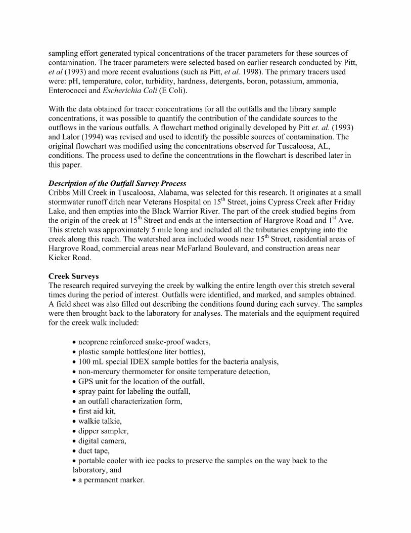
Figure 4 graphically illustrates how the detergents screening or the flowchart method is much more sensitive in identifying problems than when relying on the physical indicators alone. This graph only shows the approximate top 80% of the outfalls, as those were the only ones that had identified serious problems. Four of the outfalls always had problems for all field surveys, but the physical indicators only indicated problems at about 40 or 50% of the survey periods.

Table 12 presents the observed data relating the number of visits to an outfall (within a 1-½ year time period) to the errors associated in identifying the outfall as a problem. At least 4 outfall visits are likely needed for many intermittent conditions. If the outfall has a problem most of the time (say at least 60% of the time), four visits should result in less than a 25% error in identifying this problem. In contrast, if the outfall only has a problem infrequently (such as 20% of the time), the possible error could be much larger. In most cases, more than 5 observations seldom resulted in additional useful information.

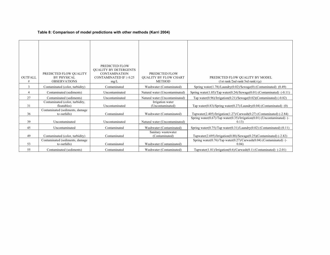
Table 8: Comparison of model predictions with other methods (Karri 2004)

OUTFALL #

PREDICTED FLOW QUALITY BY PHYSICAL

OBSERVATIONS

PREDICTED FLOW QUALITY BY DETERGENTS

CONTAMINATION CONTAMINATED IF ≥ 0.25

mg/L

PREDICTED FLOW QUALITY BY FLOW CHART

METHOD PREDICTED FLOW QUALITY BY MODEL

(1st rank/2nd rank/3rd rank) (µ)

3 Contaminated (color, turbidity) Contaminated Washwater (Contaminated) Spring water(1.78)/Laundry(0.02)/Sewage(0) (Contaminated) (0.49)

4 Contaminated (sediments) Uncontaminated Natural water (Uncontaminated) Spring water(1.05)/Tap water(0.24)/Sewage(0.01) (Contaminated) (-0.11)

27 Contaminated (sediments) Uncontaminated Natural water (Uncontaminated) Tap water(0.96)/Irrigation(0.21)/Sewage(0.02)(Contaminated) (-0.82)

31 Contaminated (color, turbidity,

floatables) Uncontaminated Irrigation water

(Uncontaminated) Tap water(0.83)/Spring water(0.27)/Laundry(0.04) (Contaminated) (0)

36 Contaminated (sediments, damage

to outfalls) Contaminated Washwater (Contaminated) Tapwater(2.405)/Irrigation(1.27)/Carwash(0.27) (Contaminated) (-2.84)

39 Uncontaminated Uncontaminated Natural water (Uncontaminated) Spring water(0.67)/Tap water(0.35)/Irrigation(0.01) (Uncontaminated) (­

0.13)

45 Uncontaminated Contaminated Washwater (Contaminated) Spring water(0.75)/Tap water(0.31)/Laundry(0.02) (Contaminated) (0.11)

49 Contaminated (color, turbidity) Contaminated Sanitary wastewater

(Contaminated) Tapwater(2.695)/Irrigation(0.88)/Sewage(0.25)(Contaminated) (-2.82)

53 Contaminated (sediments, damage

to outfalls) Contaminated Washwater (Contaminated) Spring water(0.76)/Tap water(0.27)/Carwash(0.04) (Contaminated) (­

0.04)

55 Contaminated (sediments) Contaminated Washwater (Contaminated) Tapwater(1.81)/Irrigation(0.6)/Carwash(0.1) (Contaminated) (-2.01)

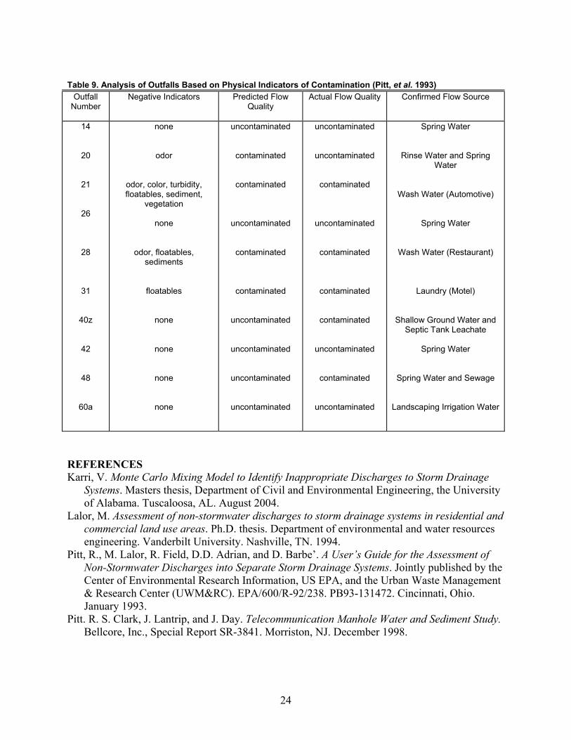
Table 9. Analysis of Outfalls Based on Physical Indicators of Contamination (Pitt, et al. 1993) Outfall

Number Negative Indicators Predicted Flow

Quality Actual Flow Quality Confirmed Flow Source

14

20

21

26

28

31

40z

42

48

60a

none

odor

odor, color, turbidity, floatables, sediment,

vegetation

none

odor, floatables, sediments

floatables

none

none

none

none

uncontaminated

contaminated

contaminated

uncontaminated

contaminated

contaminated

uncontaminated

uncontaminated

uncontaminated

uncontaminated

uncontaminated

uncontaminated

contaminated

uncontaminated

contaminated

contaminated

contaminated

uncontaminated

contaminated

uncontaminated

Spring Water

Rinse Water and Spring Water

Wash Water (Automotive)

Spring Water

Wash Water (Restaurant)

Laundry (Motel)

Shallow Ground Water and Septic Tank Leachate

Spring Water

Spring Water and Sewage

Landscaping Irrigation Water

REFERENCES Karri, V. Monte Carlo Mixing Model to Identify Inappropriate Discharges to Storm Drainage

Systems. Masters thesis, Department of Civil and Environmental Engineering, the University of Alabama. Tuscaloosa, AL. August 2004.

Lalor, M. Assessment of non-stormwater discharges to storm drainage systems in residential and commercial land use areas. Ph.D. thesis. Department of environmental and water resources engineering. Vanderbilt University. Nashville, TN. 1994.

Pitt, R., M. Lalor, R. Field, D.D. Adrian, and D. Barbe’. A User’s Guide for the Assessment of Non-Stormwater Discharges into Separate Storm Drainage Systems. Jointly published by the Center of Environmental Research Information, US EPA, and the Urban Waste Management & Research Center (UWM&RC). EPA/600/R-92/238. PB93-131472. Cincinnati, Ohio. January 1993.

Pitt. R. S. Clark, J. Lantrip, and J. Day. Telecommunication Manhole Water and Sediment Study. Bellcore, Inc., Special Report SR-3841. Morriston, NJ. December 1998.

24

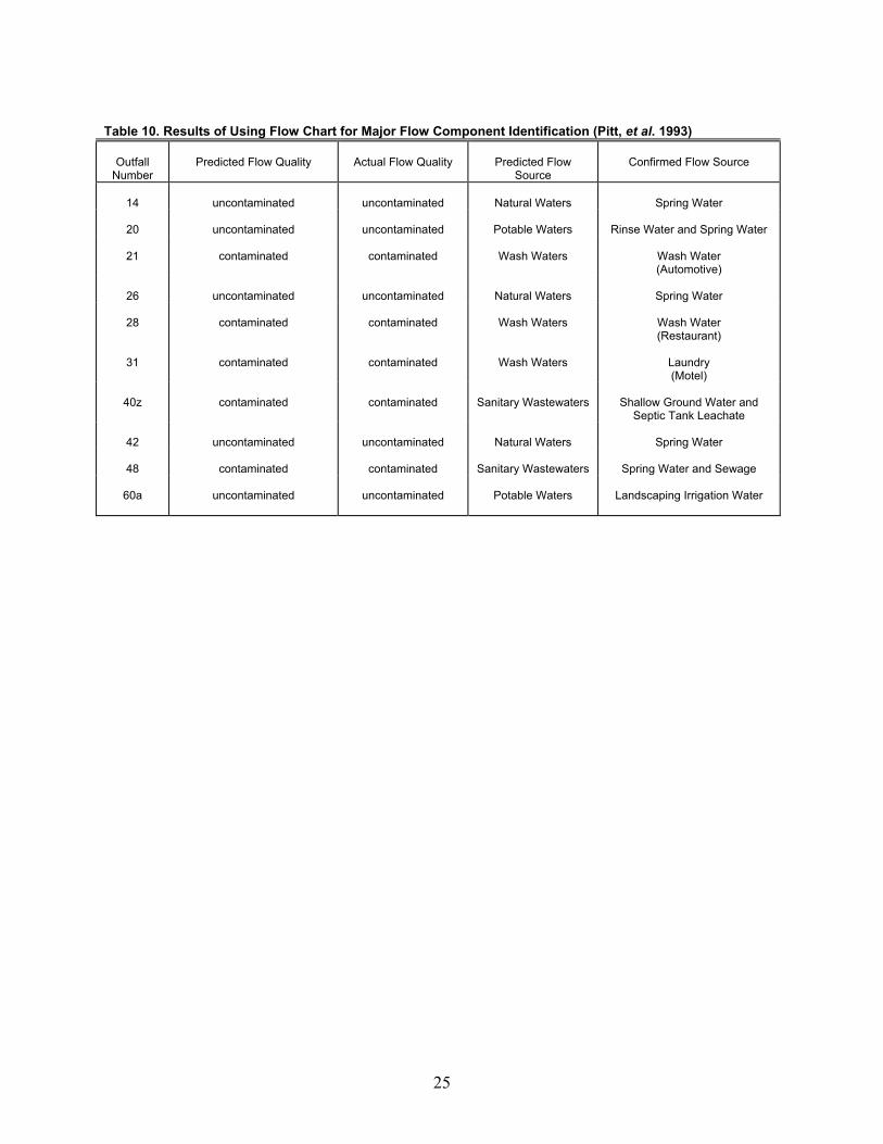
Table 10. Results of Using Flow Chart for Major Flow Component Identification (Pitt, et al. 1993)

Outfall Number

Predicted Flow Quality Actual Flow Quality Predicted Flow Source

Confirmed Flow Source

14

20

21

26

28

31

40z

42

48

60a

uncontaminated

uncontaminated

contaminated

uncontaminated

contaminated

contaminated

contaminated

uncontaminated

contaminated

uncontaminated

uncontaminated

uncontaminated

contaminated

uncontaminated

contaminated

contaminated

contaminated

uncontaminated

contaminated

uncontaminated

Natural Waters

Potable Waters

Wash Waters

Natural Waters

Wash Waters

Wash Waters

Sanitary Wastewaters

Natural Waters

Sanitary Wastewaters

Potable Waters

Spring Water

Rinse Water and Spring Water

Wash Water (Automotive)

Spring Water

Wash Water (Restaurant)

Laundry (Motel)

Shallow Ground Water and Septic Tank Leachate

Spring Water

Spring Water and Sewage

Landscaping Irrigation Water

25

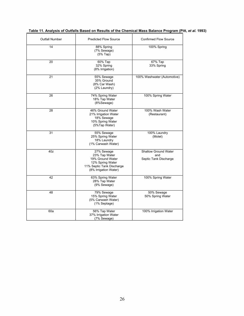
Table 11. Analysis of Outfalls Based on Results of the Chemical Mass Balance Program (Pitt, et al. 1993)

Outfall Number Predicted Flow Source Confirmed Flow Source

14 88% Spring (7% Sewage)

(5% Tap)

100% Spring

20 60% Tap 32% Spring

(8% Irrigation)

67% Tap 33% Spring

21 55% Sewage 35% Ground

(8% Car Wash) (2% Laundry)

100% Washwater (Automotive)

26 74% Spring Water 18% Tap Water

(8%Sewage)

100% Spring Water

28 46% Ground Water 21% Irrigation Water

18% Sewage 10% Spring Water

(5%Tap Water)

100% Wash Water (Restaurant)

31 55% Sewage 25% Spring Water

18% Laundry (1% Carwash Water)

100% Laundry (Motel)

40z 27% Sewage 23% Tap Water

19% Ground Water 12% Spring Water

11% Septic Tank Discharge (8% Irrigation Water)

Shallow Ground Water and

Septic Tank Discharge

42 63% Spring Water 28% Tap Water (9% Sewage)

100% Spring Water

48 79% Sewage 15% Spring Water

(5% Carwash Water) (1% Septage)

50% Sewage 50% Spring Water

60a 56% Tap Water 37% Irrigation Water

(7% Sewage)

100% Irrigation Water

26

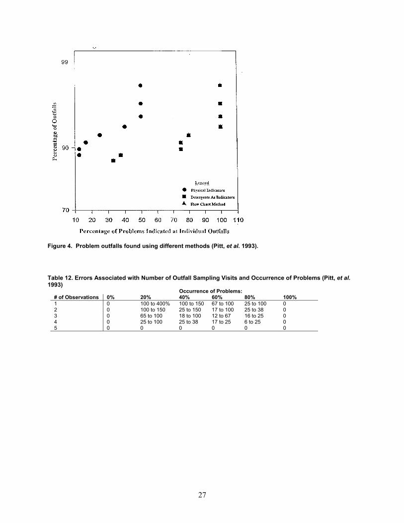
Figure 4. Problem outfalls found using different methods (Pitt, et al. 1993).

Table 12. Errors Associated with Number of Outfall Sampling Visits and Occurrence of Problems (Pitt, et al. 1993)

Occurrence of Problems: # of Observations 0% 20% 40% 60% 80% 100% 1 0 100 to 400% 100 to 150 67 to 100 25 to 100 0 2 0 100 to 150 25 to 150 17 to 100 25 to 38 0 3 0 65 to 100 18 to 100 12 to 67 16 to 25 0 4 0 25 to 100 25 to 38 17 to 25 6 to 25 0 5 0 0 0 0 0 0

27