Source-independent time-domain waveform inversion usingconvolved wavefields: Application to the encodedmultisource waveform inversion

Yunseok Choi1 and Tariq Alkhalifah1

ABSTRACT

Full waveform inversion requires a good estimation of thesource wavelet to improve our chances of a successful inversion.This is especially true for an encoded multisource time-domainimplementation, which, conventionally, requires separate-source modeling, as well as the Fourier transform of wavefields.As an alternative, we have developed the source-independenttime-domain waveform inversion using convolved wavefields.Specifically, the misfit function consists of the convolution ofthe observed wavefields with a reference trace from the modeledwavefield, plus the convolution of the modeled wavefields witha reference trace from the observed wavefield. In this case, thesource wavelet of the observed and the modeled wavefields areequally convolved with both terms in the misfit function, and

thus, the effects of the source wavelets are eliminated. Further-more, because the modeled wavefields play a role of low-passfiltering, the observed wavefields in the misfit function, thefrequency-selection strategy from low to high can be easilyadopted just by setting the maximum frequency of the sourcewavelet of the modeled wavefields; and thus, no filtering isrequired. The gradient of the misfit function is computed byback-propagating the new residual seismograms and applyingthe imaging condition, similar to reverse-time migration. In thesynthetic data evaluations, our waveform inversion yieldsinverted models that are close to the true model, but demon-strates, as predicted, some limitations when random noise isadded to the synthetic data. We also realized that an averageof traces is a better choice for the reference trace than usinga single trace.

INTRODUCTION

Waveform inversion relies on the dynamic properties of the seis-mic data to extract velocity information, whereas traveltime tomo-graphy is performed on the basis of the kinematic properties of thedata. Full waveform inversion estimates the subsurface velocitymodel by minimizing the differences between the observed andmodeled seismograms, composed of the Green’s function and thesource wavelet. Therefore, knowledge of the source wavelet of theobserved seismogram is necessary for a successful waveform inver-sion. If there is no prior information of the source wavelet, a processfor source estimation is needed for a successful waveform inversion.The source can be estimated by incorporating it as part of the

inversion. The sensitivity of the inversion to the source functioncan be assessed by taking the derivative of the misfit function withrespect to the source wavelet. Consequently, the gradient of the

misfit function with respect to the source wavelet is obtainedby back-propagating the residual seismograms (Tarantola, 1984;Zhou et al., 1997). To scale the gradient, the second derivative ofthe misfit function with respect to the source wavelet, which isexpressed as the autocorrelation of Green’s function (Pratt, 1999;Shin et al., 2007), is required. Instead of the exact Green’s function,we typically use the band-limited Green’s function or the Fouriertransformed wavefields to apply the full-Newton method (Lines andTreitel, 1984) for source-estimation in the time-domain waveforminversion.Recently, Krebs et al. (2009) suggested an encoded multisource

approach to dramatically reduce the computational cost of time-domain, full-waveform inversion. In their approach, each sourcefunction (i.e., function of source time and position) used for forwardmodeling is randomly multiplied by either þ1 or −1 and gathered

Manuscript received by the Editor 12 July 2010; revised manuscript received 8 March 2011; published online 14 November 2011.1King Abdullah University of Science and Technology, Physical Science and Engineering Division, Thuwal, Saudi Arabia. E-mail: yunseok.choi@

kaust.edu.sa; tariq.alkhalifah@kaust.edu.sa.© 2011 Society of Exploration Geophysicists. All rights reserved.

R125

GEOPHYSICS. VOL. 76, NO. 5 (SEPTEMBER-OCTOBER 2011); P. R125–R134, 11 FIGS.10.1190/GEO2010-0210.1

Dow

nloa

ded

10/1

1/15

to 1

09.1

71.1

37.2

10. R

edis

trib

utio

n su

bjec

t to

SEG

lice

nse

or c

opyr

ight

; see

Ter

ms

of U

se a

t http

://lib

rary

.seg

.org

/

into a super-source function for the simultaneous-source modeling.Another important step in their method is varying the set of randomnumbers used at each iteration to reduce crosstalk artifacts. How-ever, because the gradient of the misfit function with respect to thesource wavelet is just the back-propagated wavefield (not includingcrosstalk artifacts), the process of varying the random number set ateach iteration complicates the estimation of the source wavelet.Therefore, we need a few additional separate-source modeling andFourier transforms of wavefields for a successful source estimationin the encoded multisource time-domain waveform inversion.Because we need only two modeling applications for each gradientcalculation in the multisource waveform inversion, a few additionalmodeling steps are still costly in the multisource waveforminversion.The cross-convolved wavefields suggested in this paper can help

us avoid the need for source-estimation in the multisource time-domain waveform inversion because in this case, the effect of thesource wavelet is removed at each iteration in source-independentwaveform inversion. So far, many source-independent algorithmsfor waveform inversion have been developed in the frequency do-main (Lee and Kim, 2003; Zhou and Greenhalgh, 2003; Choi et al.,2005; Cheong et al., 2006; Xu et al., 2006). There are two kinds ofsource-independent algorithms: one based on the deconvolution andone based on the convolution approach. In the deconvolution-basedapproach, the wavefields are normalized by a reference wavefieldand expressed as a ratio of Green’s functions in the frequencydomain (Lee and Kim, 2003; Xu et al., 2006) in which the sourcefunction gets canceled. On the other hand, Choi et al. (2005) andCheong et al. (2006) suggest the convolution-based approach forthe source-independent waveform inversion in which the wavefieldsare multiplied by a cross-reference wavefield in the frequencydomain. Because the deconvolution-based approaches for time-domain waveform inversion demands additional Fourier transformsand careful treatment of the division involved, we prefer a morestraightforward convolution-based approach.

In this paper, we apply the convolution-based method to theencoded multisource time-domain waveform inversion method. Wefirst convolve the observed wavefields with a reference trace of themodeled wavefield, and vice versa, we convolve the modeled wave-fields with a reference trace of observed wavefield and construct themisfit function using these convolved wavefields. The referencewavefield can be a single trace or an average of all traces in theshot gather. In the misfit function, both source wavelets of theobserved and the modeled wavefields are equally convolved in bothterms. Therefore, their effect is removed because of the linearbehavior of convolution. Another important feature of this misfitfunction is that the modeled wavefields act as a low-pass filter ofthe observed wavefields based on the frequency range of the sourceused for modeling. Therefore, we can easily employ a frequency-selection strategy moving from low to high frequencies for wave-form inversion (Bunks et al., 1995; Sirgue and Pratt, 2004) just bysetting the maximum frequency of the source wavelet of the mod-eled wavefields. In addition, we can also obtain the gradient ofmisfit function with respect to velocities by using the back-propagation algorithm based on the adjoint-state technique (Laily,1983; Tarantola, 1984; Gauthier et al., 1986; Zhou et al., 1995;Pratt et al., 1998; Shin and Min, 2006; Choi et al., 2008).We start by introducing the new misfit function using the con-

volved wavefields, and provide the expression of the gradient of themisfit function using the back-propagation algorithm. We thenadapt this expression for multisource waveform inversion. Finally,to test our algorithm, we apply our waveform inversion with asingle-trace reference and with an average-of-traces reference. Wethen compare these choices to the known-source inversion approachfor noise-free and random noise-added synthetic data generatedwith the Marmousi2 model (Martin et al., 2002).

THEORY

Key elements of waveform inversion are the misfit (objective)function that we seek to minimize, the minimization (optimization)tool, and the scaling and regularization required to make the mini-mum unique and reachable. In this section, we will develop theinversion for our suggested convolutional approach, consideringmultisources.

Misfit function using the convolved wavefields

The misfit function E for waveform inversion is generally definedas the l 2 norm of the residuals between the modeled data and theobserved:

E ¼Xnsi

Xnrj

kui;j − di;jk2; (1)

where ns and nr are the number of shots and receivers, respectively;and ui;j and di;j are traces of the modeled and the observed datafor the ith shot and jth receiver, respectively. If we express ui;jand di;j as the convolutions of the Green’s functions and the sourcewavelets, the misfit function takes the following form:

E ¼Xnsi

Xnrj

kgui;j � su − gdi;j � sdk2; (2)

where g and s are Green’s function and source wavelet, respectively;the symbol � represents the convolution process, and superscripts

Figure 1. (a) The Marmousi2 velocity model and (b) the startingvelocity model for the waveform inversions. The velocities ofthe starting model linearly increase with depth from 1.5 to 4 km/s.

R126 Choi and Alkhalifah

Dow

nloa

ded

10/1

1/15

to 1

09.1

71.1

37.2

10. R

edis

trib

utio

n su

bjec

t to

SEG

lice

nse

or c

opyr

ight

; see

Ter

ms

of U

se a

t http

://lib

rary

.seg

.org

/

u and d stand for the modeled and observed data, respectively. Inwaveform inversion, the subsurface model parameters are updatedby minimizing the misfit function E in equation 2. Theoretically,the source wavelet (sd) could be estimated in the process of mini-mizing the misfit function as well.To avoid the source estimation in the time-domain waveform

inversion, we suggest a source-independent algorithm using thecross-convolved wavefileds. For each shot gather, the modeledwavefields are convolved with a reference trace from the observedwavefield, and the observed wavefields are convolved with a refer-ence trace from the modeled wavefield. As a result, the new misfitfunction is defined by

E ¼Xnsi

Xnrj

kui;j � di;k − di;j � ui;kk2; (3)

where ui;k and di;k are the reference traces from the modeled andthe observed data, respectively, at the kth receiver position. Wecan express equation 3 using the convolution of the Green’s func-tion with the source wavelet as follows:

E ¼Xnsi

Xnrj

kgui;j � gdi;k � su � sd − gdi;j � gui;k � su � sdk2: (4)

In equation 4, the new source wavelet (su � sd) isconvolved in both terms equally. Based on thelinear nature of the convolution process, theeffect of the sources is removed from the misfitfunction. Thus, the misfit function becomessource independent and its estimation is nolonger needed for waveform inversion.

Calculation of the gradientof the misfit function

The l 2 norm in equation 3 can be rewritten as adot product:

E ¼Xnsi

Xnrj

1

2½ðui;j � di;k − di;j � ui;kÞ

· ðui;j � di;k − di;j � ui;kÞ�: (5)

The gradient of the misfit function is obtained bytaking the derivative of equation 5 with respect tothe mth model parameter pm as follows:

∂E∂pm

¼Xnsi

Xnrj

��∂ui;j∂pm

� di;k�

· ri;j

−�di;j �

∂ui;k∂pm

�· ri;j

�; (6)

where ri;j ¼ ui;j � di;k − di;j � ui;k .We recast the dot product and the convolution

in the first term on the right-hand side ofequation 6 in an integral form as

�∂ui;j∂pm

� di;k�

· ri;j

¼Z

∞

−∞

Z∞

−∞

�∂ui;j∂pm

ðt − τÞdi;kðτÞri;jðtÞ�dτdt: (7)

If we set t − τ ¼ ξ, then dτ ¼ −dξ, and equation 7 is rewritten as

�∂ui;j∂pm

� di;k�

· ri;j ¼ −Z

∞

−∞

∂ui;j∂pm

ðξÞ�Z

∞

−∞di;kðt − ξÞri;jðtÞdt

�dξ

¼ −Z

∞

−∞

∂ui;j∂pm

ðξÞr 0i;jðξÞdξ: (8)

In equation 8, r 0i;jðξÞ is the crosscorrelation of the residualseismogram and the reference traces from the observed wavefield.Equation 8 can be expressed as a dot product between the partial-derivative wavefield (∂ui;j∕∂pm) and the first correlated-residualseismogram (r 0i;j), which has the same general form as in the conven-tional formulas of the gradient of the misfit function for full wave-form inversion.

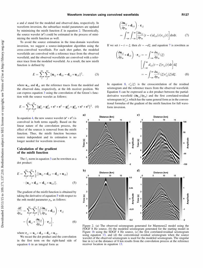
Figure 2. (a) The observed seismogram generated for Marmousi2 model using theFDGF 8 Hz source, (b) the modeled seismogram generated for the starting model inFigure 1b using the SDGF 4 Hz source, (c) the first correlated-residual seismogramusing equation 13, and (d) the conventional residual seismogram when the sourcewavelet of the observed seismogram is used for the modeled seismogram. The singularline in (c) at the distance of 8 km results from the convolution process at the referencereceiver location in equation 13.

Waveform inversion using convolved wavefields R127

Dow

nloa

ded

10/1

1/15

to 1

09.1

71.1

37.2

10. R

edis

trib

utio

n su

bjec

t to

SEG

lice

nse

or c

opyr

ight

; see

Ter

ms

of U

se a

t http

://lib

rary

.seg

.org

/

In equation 8, ∂ui;j∕∂pm can be obtained from the convolution ofthe up-going Green’s function, gux;j, and the virtual-source, v

ui;x (Pratt

et al., 1998; Shin et al., 2001), where x represents the variable ofsubsurface model space. For a constant-density acoustic wave equa-tion, vui;x is expressed as ð2∕p3mÞ × ð∂2ui;x∕∂t2Þ or 2pmΔui;x based onthe Born approximation where p represents velocity. The expressionfor the virtual source depends on the type of wave equation. Theterm “virtual source” is used by Pratt et al. (1998) and Shinet al. (2001). The virtual source is similar to the weighted down-going Green’s function convolved with the source wavelet (orthe weighted forward-propagated source wavefield). Therefore,equation 8 is also regarded as a Born-approximation-type inversion.Using the convolution of gux;j and vui;x, equation 8 is rewritten as

�∂ui;j∂pm

� di;k�

· ri;j ¼ −Z

∞

−∞

�Z∞

−∞vui;xðξ − τÞgux;jðτÞdτ

�

r 0i;jðξÞdξ: (9)

Again, by setting ξ − τ ¼ t and dτ ¼ −dt, equation 9 becomes

�∂ui;j∂pm

� di;k�

· ri;j ¼Z

∞

−∞

�Z∞

−∞vui;xðtÞgux;jðξ − tÞdt

�

r 0i;jðξÞdξ ¼Z

∞

−∞vui;xðtÞ�Z

∞

−∞gux;jðξ − tÞr 0i;jðξÞdξ

�dt: (10)

TheGreen’s function, gux;j, satisfies the reciprocity theorem, and thus,gux;j ¼ guj;x. Therefore, the crosscorrelation, ∫ gux;jðξ − tÞr 0i;jðξÞdξ,can be regarded as a back-propagation of the first correlated-residual seismogram r 0i;j. Because the back-propagated wavefield,∫ gux;jðξ − tÞr 0i;jðξÞdξ, in equation 10 is time-reversed with respectto the variable t, equation 10 can be regarded as the zero-lag convo-lution of the back-propagated wavefield and the virtual source.Therefore, this equation is equivalent to the imaging conditionfor reverse-time migration, except for back-propagating the firstcorrelated-residual seismogram instead.The second term in equation 6 can be also formulated in a similar

fashion, resulting in

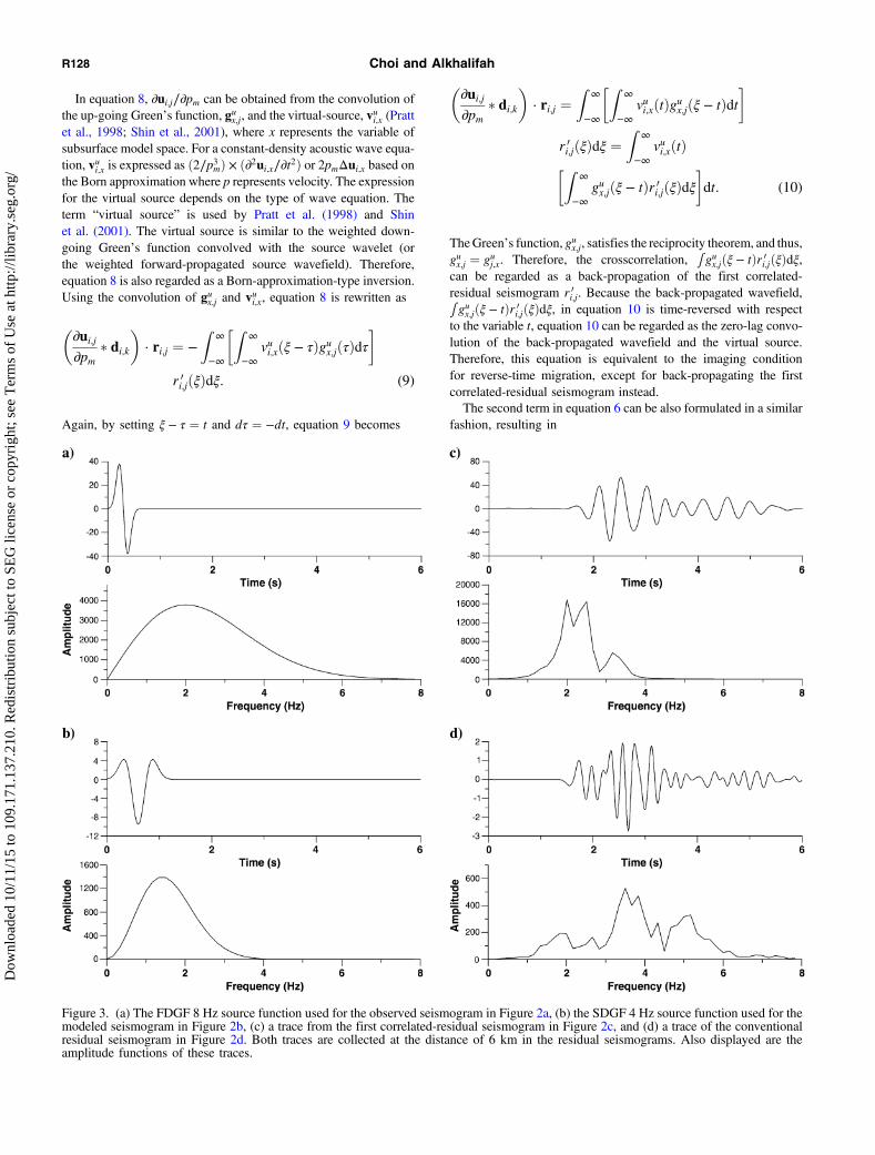
Figure 3. (a) The FDGF 8 Hz source function used for the observed seismogram in Figure 2a, (b) the SDGF 4 Hz source function used for themodeled seismogram in Figure 2b, (c) a trace from the first correlated-residual seismogram in Figure 2c, and (d) a trace of the conventionalresidual seismogram in Figure 2d. Both traces are collected at the distance of 6 km in the residual seismograms. Also displayed are theamplitude functions of these traces.

R128 Choi and Alkhalifah

Dow

nloa

ded

10/1

1/15

to 1

09.1

71.1

37.2

10. R

edis

trib

utio

n su

bjec

t to

SEG

lice

nse

or c

opyr

ight

; see

Ter

ms

of U

se a

t http

://lib

rary

.seg

.org

/

−�di;j �

∂ui;k∂pm

�· ri;j ¼

Z∞

−∞vui;xðtÞ

�Z∞

−∞gux;kðξ − tÞr 0 0i;jðξÞdξ

�dt; (11)

where

r 0 0i;jðξÞ ¼ −Z

∞

−∞½di;jðt − ξÞ · ri;jðtÞ�dt: (12)

In equations 11 and 12, we note that the second correlated-residualseismogram r 0 0i;j should be back-propagated only at the kth referencereceiver position.Consequently, the gradient of the misfit function for the source-

independent time-domain waveform inversion is computed byback-propagating the first correlated-residual seismogram,

r 0i;j ¼ di;k ⊗ ðui;j � di;k − di;j � ui;kÞ; (13)

at each jth receiver position, and the second correlated-residualseismogram,

r 0 0i;j ¼ −di;j ⊗ ðui;j � di;k − di;j � ui;kÞ; (14)

back-propagated only at the kth reference receiver position.The first and second correlated-residual seismograms are back-propagated at the same time, which requires only one modelingstep. In equations 13 and 14, ⊗ stands for the crosscorrelationoperation. In equation 13, the kth trace of the observed data iscorrelated to all traces of the residual seismogram, whereas inequation 14, the crosscorrelation is done trace by trace betweenthe observed data and the residual seismogram. In practice, the sec-ond correlated-residual seismogram in equation 14 can be summedacross receivers to make a single-trace that is back-propagated at thekth receiver position. In theory, the position of the reference trace isnot important. However, in practice, our experimentations suggestthat a near-offset trace is a better reference than a far-offset trace.The flowchart of our waveform inversion is very similar to the oneof Krebs et al. (2009) except for the back-propagation of the firstand second correlated-residual seismograms.We note that the convolution of the observed and modeled data

with reference traces affect both amplitude and phase information.However, in the residual seismograms, the correlation steps cancelout any time shift introduced by the convolution. Yet, these convo-lution and crosscorrelation operations could increase the nonlinear-ity of the problem, resulting in slower convergence and increasedsensitivity to the presence of local minima. Therefore, our methodmight require more accurate starting models and better multiscalestrategies.

Application to encoded multisourcewaveform inversion

The encoded multisource method of Krebs et al. (2009) wasdeveloped to reduce the computational cost of the time-domain,full-waveform inversion. In their method, two simulations are alsoneeded for each gradient calculation: one for the simultaneous for-ward extrapolation of the encoded shots and one for the backwardextrapolation of the encoded residual seismograms. Each sourcefunction is randomly multiplied by either þ1 or −1 and summedinto a super-source gather. The set of random numbers is regener-ated at each iteration to reduce crosstalk artifacts arising from the

convolution of the back-propagated wavefield and the forwardmodeled wavefield (or virtual-source wavefield in our examples).However, because the gradient of the misfit function with respectto the source wavelet is just the back-propagated wavefield (notincluding crosstalk artifacts), different random numbers generateentirely different gradients with respect to the source wavelet at eachiteration. Therefore, source estimation using the encoded shotsapproach would require some extra computational steps that oursource-independent scheme would not. Note that when we use ourapproach with the encoded multisource scheme, single-shot gathersare simply replaced with encoded multishot gathers.

Scaling and optimization

To compensate for the geometrical spreading effects, we scale thegradient using the diagonal term of the Pseudo-Hessian matrix(Shin et al., 2001), which is written as

Figure 4. The observed (a) and modeled (b) encoded seismograms.The Marmousi2 model is used for the observed seismogram in(a) with the FDGF 8 Hz source. The model in Figure 1b is usedfor the modeled seismogram in (b) with the SDG 2 Hz source.

Waveform inversion using convolved wavefields R129

Dow

nloa

ded

10/1

1/15

to 1

09.1

71.1

37.2

10. R

edis

trib

utio

n su

bjec

t to

SEG

lice

nse

or c

opyr

ight

; see

Ter

ms

of U

se a

t http

://lib

rary

.seg

.org

/

Hpseudo ¼ diag½VTVþ λI�; (15)

where each column of V is a virtual-source vector vui;x, which isdescribed below equation 8, superscript T denotes the transposeoperation, λ is a damping factor, and I is the identity matrix. Wealso use the conjugate-gradient method (Gill et al., 1981) to updatethe model parameters in which the search direction qðnÞ at the ðnÞthiteration is expressed as a linear combination of the scaled gradientbðnÞ and the search direction qðn−1Þ:

qðnÞ ¼ −bðnÞ þ ðbðnÞÞTbðnÞðbðn−1ÞÞTbðn−1Þ q

ðn−1Þ: (16)

Consequently, the model parameter pðnÞ is updated using the searchdirection as

pðnÞ ¼ pðn−1Þ þ αðnÞqðnÞ; (17)

where αðnÞ is the step length at the ðnÞth iteration. To obtain a properstep length, we could employ a line-search method, but, for sim-plicity, we fix the value of the step length. The value is fixed to a

relatively small step size that worked fine for all our numericalexperiments.

SYNTHETIC EXAMPLES

We first generate synthetic data for the Marmousi2 model(Martin et al., 2002) by using a time-domain finite-difference mod-eling technique to solve the constant-density acoustic wave equa-tion. We also use an absorbing boundary condition (Clayton andEngquist, 1977), and the first derivative of a Gaussian function witha maximum frequency of 8 Hz (FDGF 8 Hz) for the source wavelet.Then, we test our waveform inversion algorithm on a generated 2Dsynthetic data set. Figure 1 shows the P-wave velocities for theMarmousi2 model and our starting guess for the waveform inver-sion tests. The grid interval for both horizontal and vertical direc-tions is 20 m. We position 212 shots every 80 m at a 20-m depth andreceivers at all grid points at a 20-m depth as well. The data record-ing time is 6 s. For the modeled data, we use the second derivative ofa Gaussian function (SDGF) for the source wavelet. In these syn-thetic examples, we use either a single trace or an average of traces(in a shot gather) as our reference trace. Although a near-offset traceis a preferred for the inversion of single shots, a different strategy isused when encoded-shots are inverted. In practice, we choose the

Figure 5. The inverted velocity models when using (a) the SDGF 2 Hz, (b) the SDGF 4 Hz, (c) the SDGF 6 Hz, and (d) the SDGF 8 Hz sourcesfor the modeled seismogram. Each inverted model (a–d) is obtained after 200 iterations based on a single-trace reference and used as a startingmodel for the next frequency. Finally, the inverted model of the last inversion step in (d) is obtained after 800 iterations. (e) The final invertedmodel after 800 iterations using an average trace reference, and (f) the inverted model obtained by conventional multisource waveforminversion using the known-source.

R130 Choi and Alkhalifah

Dow

nloa

ded

10/1

1/15

to 1

09.1

71.1

37.2

10. R

edis

trib

utio

n su

bjec

t to

SEG

lice

nse

or c

opyr

ight

; see

Ter

ms

of U

se a

t http

://lib

rary

.seg

.org

/

trace at a distance of ð120þ 80iÞ m, where i is the iteration number(if i is greater than the number of shots, we subtract the number ofshots from i for choosing a reference trace), and for theaverage trace, we sum all receiver traces and divide it by the numberof traces.

A look at the correlated-residual seismogram

To demonstrate some of the features of the newly suggestedresidual seismograms, we compare them with the conventional onesby first using the single-source inversion approach. Because the sec-ond correlated-residual seismogram is regarded as a single trace inequation 14, we consider only the first correlated-residual seis-mogram in this section. Figure 2a shows the observed seismogramgenerated for the Marmousi2 model using the FDGF 8 Hz source,Figure 2b shows the modeled seismogram for the starting model inFigure 1 using the SDGF 4 Hz source, and Figure 2c and 2d showsthe residual seismograms. Figure 3 shows the FDGF 8 Hz sourcefunction used for the observed seismogram, the SDGF 4 Hz sourcefunction used for the modeled seismogram, and the traces of theresidual seismograms of Figure 2c and 2d at a distance of 6 km.When using the FDGF 8 Hz source for both the observed andmodeled seismograms, the conventional seismogram (Figure 2d)contains only reflected and the refracted waves. However, eventhough different source wavelets (Figure 3a and 3b) are used, thefirst correlated-residual seismogram (Figure 2c) does not containdirect waves and shows similar features to those in the residual seis-mogram (Figure 2d) for which the exact source (FDGF 8 HZ) wasused. From this comparison, we realize two features of the firstcorrelated-residual seismogram. First, it has similar features to theknown-source conventional residual seismogram, despite the factthat we did not require the knowledge of the source. Second, thefirst correlated-residual seismogram is a low-pass filtered versionof the conventional residual seismogram for a known source, whichcan be observed clearly in Figure 3c and 3d by comparing theiramplitude spectra. The trace corresponding to the conventionalresidual seismogram in Figure 3c has a maximum frequency of8 Hz, whereas the trace extracted from the first correlated-residualseismogram, has a maximum frequency of 4 Hz. This is because themodeled seismogram plays the additional role of a low-pass filterapplied to the observed seismogram. Therefore, we can easilyemploy a frequency-selection strategy moving from low to high fre-quencies (Bunks et al., 1995; Sirgue and Pratt, 2004) by select-ing the maximum frequency of the source wavelets of the modeledseismograms.

Noise-free synthetic data examples

In the following waveform inversion example, we invert encodedseismograms. Also, we adopt a frequency-selection strategy movingfrom low to high frequencies (Bunks et al., 1995; Sirgue and Pratt,2004). For this frequency-selection strategy,we use the SDGF sourcefor the modeled seismogram and set its maximum frequency to 2, 4,6, and 8 Hz.We ran 200 iterations for each frequency band, using theresult of the previous scale as a starting guess for the next. Theamplitudes of the SDGF increase with the increase in the maximumfrequencies to maintain constant wavelet energy. It also implies thatthe peak frequencies increase as we increase the maximum frequen-cies of the source wavelets. Figure 4a shows the observed encodedseismogram using the FDGF 8 Hz source for one realization of the

encoding function and Figure 4b shows the encoded super-shotmod-eled seismogram using the SDGF 2Hz source for the same encodingfunction as in Figure 4a. The modeled seismogram is computed byusing the starting model in Figure 1b. The random signal appearingon the top of the seismograms in Figure 4 explicitly displays the pat-tern of the random numbers sequence used to create the encodedshots and seismograms. Figure 5a, 5b, 5c, and 5d show the invertedmodels when using the SDGF 2 Hz, SDGF 4 Hz, SDGF 6 Hz, andSDGF8Hz sources for themodeled seismograms, respectively. Eachinvertedmodel uses a single-reference trace. Figure 5e also shows thefinal inverted model using an average trace reference and Figure 5fshows the inverted model obtained by the encoded multisourcewaveform inversion using the known source (EMSWIKS; FDGF8 Hz is used for the modeled data). If we choose an average tracereference in the randomly encoded multisource waveform inversion,the effect of the second correlated residual is much weaker than thatof the first correlated residual becausewe sum the randomly encodedresidual seismogram across receivers and divide it by the number ofreceivers for the second correlated residual. Therefore, for conveni-ence, we only back-propagate the first correlated-residual seis-mogram as defined in equation 13 in the example of the average tracereference. We can clearly observe the overall convergence of the in-version and the value of each frequency step up on the resolution.

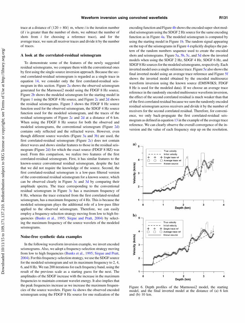
Figure 6. Depth profiles of the Marmousi2 model, the startingmodel, and the final inverted model at the distance of (a) 6 kmand (b) 10 km.

Waveform inversion using convolved wavefields R131

Dow

nloa

ded

10/1

1/15

to 1

09.1

71.1

37.2

10. R

edis

trib

utio

n su

bjec

t to

SEG

lice

nse

or c

opyr

ight

; see

Ter

ms

of U

se a

t http

://lib

rary

.seg

.org

/

Figure 6 shows corresponding depth profiles for the Marmousi2model, the starting model, and the final inverted models at locations6 and 10 km. In Figure 6, we observe that the shallow part of the finalinverted model is comparable to the true model, whereas the deeperpart appears smoother. From Figures 5 and 6, we note that the in-verted models using our algorithm (a single-trace reference andan average trace reference) show some limitations in resolution(e.g., the part at a horizontal distance of 12 km and a depth of1.5 km in Figure 5) when compared with the inverted model ofthe EMSWIKS. This is because the modification of amplitudeand phase of original data caused by convolution in the objectivefunction affects the results of inversion. Figure 7 shows the historyof the misfit functions for our different methods for the first fre-quency band (0–2 Hz) (each normalized to one). Figure 7 shows thatour source-independent approach has more severe fluctuations thanthat of the EMSWIKS. An alternate definition of the misfit function(especially, the convolution operation in the misfit function) and achoice of a different reference trace might alter this conclusion. Eventhough the history of the misfit function of our algorithm showssevere fluctuations, the inverted models of our algorithm convergesmoothly to the right answer, as Figure 8 demonstrates: the valueof the model-fit decreases as the number of iterations increases.

Although the EMSWIKS shows a general bettermodel-fit, ourwave-form inversion results converged well to the true model. In fact, theinversion using an average trace reference shows a better model-fitresult than that using a single-trace reference, in agreement with the

Figure 9. Representative synthetic seismograms contaminated withrandom noise of S/N of 34 dB.

Figure 10. The inverted models after 800 iterations using (a) single-trace reference, (b) average trace reference, and (c) known-sourcefor the random noise data of S/N of 34 dB. The same source waveletand frequency-selection strategy as in the previous inversion exam-ple are used here.

Figure 7. The history of the misfit function for the noise-free datain the first inversion step using the SDGF 2 Hz source for source-independent inversions. All values of the misfit function are normal-ized by the value of the 1st iteration.

Figure 8. The history of the model-fit between the Marmousi2model and the inverted models for the noise-free data.

R132 Choi and Alkhalifah

Dow

nloa

ded

10/1

1/15

to 1

09.1

71.1

37.2

10. R

edis

trib

utio

n su

bjec

t to

SEG

lice

nse

or c

opyr

ight

; see

Ter

ms

of U

se a

t http

://lib

rary

.seg

.org

/

result of Xu et al. (2006). Therefore, our waveform inversion algo-rithm works well with the noise-free synthetic data.

Random noise added to the observed data

To test our waveform inversion algorithm in more realistic con-ditions, we add random noise to the observed (synthetic) data.Again, and for comparison purposes, we apply both our inversionand the EMSWIKS algorithms to the noisy data. Figure 9 shows thesynthetic seismogram in Figure 2a contaminated with random noisewith a signal-to-noise ratio (S/N) of 34 dB. Figure 10 shows theinverted models at 800th iteration for the noisy data. The samesource wavelet and frequency-selection strategy used in the pre-vious inversion example are used here. Figure 11 shows the historyof the model-fit between the Marmousi2 model and the invertedmodels for the noisy synthetic data inversion. From these figures,we note that the inverted models of the EMSWIKS and the averagetrace reference show good convergence, whereas the invertedmodel of a single-trace reference does not. We think that the averagetrace strategy mitigates the effect of random noise by summing allreceiver traces together, whereas a single trace does not. Therefore,we can conclude that, for our algorithm, averaging traces is a betterstrategy for the reference than selecting a single one. Still, we notethat our waveform inversion algorithm is sensitive to random noise,and that noise reduction is required before inversion.

CONCLUSIONS

We developed a source-independent algorithm using convolvedwavefields. Our waveform inversion algorithm can be applied toboth the separate-source and multisource waveform inversion. Themisfit function for each shot gather consists of convolving theobserved wavefield with a reference trace from the modeled wave-field and the modeled wavefield with a reference trace from theobserved wavefield. The reference trace can be a single-chosentrace or an average of traces within a shot gather. Because the sourcewavelets of the observed and modeled wavefields are equally con-volved in both terms in the misfit function, its influence is readilyremoved. Furthermore, the modeled wavefields play the role of alow-pass filter in the misfit function that make the frequency-selection strategy for waveform inversion easy to set up by adjustingthe maximum frequency of the source wavelet. In addition, to

compute the gradient of the misfit function with respect to the sub-surface velocities, we use the back-propagation method based onthe adjoint-state technique.The synthetic examples showed that, without estimating the

source wavelet, the inverted model obtained from our waveforminversion algorithm is compatible with the true model for the noise-free synthetic data. We also note that the average of traces is a betterchoice for reference trace than a single trace. However, if we includerandom noise, the inverted model shows some limitations inresolution and the choice of the reference trace (single or average)affect the inversion results. More study is required to mitigate thisproblem. Nevertheless, because multisource time-domain wave-form inversion requires the knowledge of the source wavelet, thissource-independent approach can be an alternative.

ACKNOWLEDGMENTS

We are grateful to King Abdullah University of Science andTechnology for financial support. We thank the assistant editor, theassociate editor, and the reviewers for their critical and helpfulreview of the manuscript.

REFERENCES

Bunks, C., F. M. Saleck, S. Zaleski, and G. Chavent, 1995, Multi-scale seismic waveform inversion: Geophysics, 60, 1457–1473, doi:10.1190/1.144388.

Cheong, S., S. Pyun, and C. Shin, 2006, Two efficient steepest-descentalgorithm for source signature-free waveform inversion: Journal ofSeismic Exploration, 14, 335–348.

Choi, Y., D. J. Min, and C. Shin, 2008, Frequency-domain full waveforminversion using the new pseudo-Hessian matrix: Experience of elasticMarmousi-2 synthetic data: Bulletin of the Seismological Society ofAmerica, 98, 2402–2415, doi: 10.1785/0120070179.

Choi, Y., C. Shin, D. J. Min, and T. Ha, 2005, Efficient calculation of thesteepest descent direction for source-independent seismic waveforminversion: An amplitude approach: Journal of Computational Physics,208, 455–468, doi: 10.1016/j.jcp.2004.09.019.

Clayton, R., and B. Engquist, 1977, Absorbing boundary conditions foracoustic and elastic wave equations: Bulletin of the Seismological Societyof America, 67, 1529–1540.

Gauthier, O., J. Virieux, and A. Tarantola, 1986, Two-dimensional nonlinearinversion of seismic waveforms: Numerical results: Geophysics, 51,1387–1403, doi: 10.1190/1.1442188.

Gill, P. E., W. Murray, and M. Wright, 1981, Practical optimization:Academic Press, Inc.

Krebs, J. R., J. E. Anderson, D. Hinkley, R. Neelamani, S. Lee,A. Baumstein, and M. D. Lacasse, 2009, Fast full-wavefield seismicinversion using encoded sources: Geophysics, 74, no. 6, WCC177–WCC188, doi: 10.1190/1.3230502.

Lailly, P., 1983, The seismic inverse problem as a sequence of before stackmigration, in J. B., Bednar, R. Rednar, E. Robinson, and A. Weglein, eds.,Conference on inverse scattering: Theory and application: Society forIndustrial and Applied Mathematics.

Lee, K. H., and H. J. Kim, 2003, Source-independent full-waveforminversion of seismic data: Geophysics, 68, 2010–2015, doi: 10.1190/1.1635054.

Lines, L. R., and S. Treitel, 1984, A review of least-squares inversion andits application to geophysical problems: Geophysical Prospecting, 32,159–186, doi: 10.1111/j.1365-2478.1984.tb00726.x.

Martin, G. S., K. J. Marfurt, and S. Larsen, 2002, Marmousi-2: An updatedmodel for the investigation of AVO in structurally complex areas: 72ndAnnual International Meeting, SEG, Expanded Abstracts, 1979–1982.

Pratt, R. G., 1999, Seismic waveform inversion in the frequency domain,Part 1: Theory and verification in a physical scale model: Geophysics,64, 888–901, doi: 10.1190/1.1444597.

Pratt, R. G., C. Shin, and G. J. Hicks, 1998, Gauss-Newton and full Newtonmethods in frequency domain seismic waveform inversion: GeophysicalJournal International, 133, 341–362, doi: 10.1046/j.1365-246X.1998.00498.x.

Shin, C., S. Jang, and D. J. Min, 2001, Improved amplitude preservation forprestack depth migration by inverse scattering theory: GeophysicalProspecting, 49, 592–606, doi: 10.1046/j.1365-2478.2001.00279.x.

Shin, C., and D. J. Min, 2006, Waveform inversion using a logarithmicwavefield: Geophysics, 71, no. 3, R31–R42, doi: 10.1190/1.2194523.

Figure 11. The history of the model-fit between the Marmousi2model and the inverted models for the random noisy data withS/N of 34 dB.

Waveform inversion using convolved wavefields R133

Dow

nloa

ded

10/1

1/15

to 1

09.1

71.1

37.2

10. R

edis

trib

utio

n su

bjec

t to

SEG

lice

nse

or c

opyr

ight

; see

Ter

ms

of U

se a

t http

://lib

rary

.seg

.org

/

Shin, C., S. Pyun, and J. B. Bednar, 2007, Comparison of waveform inver-sion, Part 1: Conventional wavefield vs logarithmic wavefield: Geophy-sical Prospecting, 55, 449–464, doi: 10.1111/j.1365-2478.2007.00617.x.

Sirgue, L., and R. G. Pratt, 2004, Efficient waveform inversion andimaging: A strategy for selecting temporal frequencies: Geophysics,69, 231–248, doi: 10.1190/1.1649391.

Tarantola, A., 1984, Inversion of seismic reflection data in the acousticapproximation: Geophysics, 49, 1259–1266, doi: 10.1190/1.1441754.

Xu, K., S. A. Greenhalgh, and M. Wang, 2006, Comparison of source-independent methods of elastic waveform inversion: Geophysics, 71,no. 6, R91–R100, doi: 10.1190/1.2356256.

Zhou, B., and S. A. Greenhalgh, 2003, Crosshole seismic inversion withnormalized full-waveform amplitude data: Geophysics, 68, 1320–1330,doi: 10.1190/1.1598125.

Zhou, C., W. Cai, Y. Luo, G. T. Schuster, and S. Hassanzadeh,1995, Acoustic wave-equation traveltime and waveform inversion ofcross hole seismic data: Geophysics, 60, 765–773, doi: 10.1190/1.1443815.

Zhou, C., G. T. Schuster, S. Hassanzadeh, and J. M. Harris, 1997, Elasticwave equation traveltime and waveform inversion of crosswell data:Geophysics, 62, 853–868, doi: 10.1190/1.1444194.

R134 Choi and Alkhalifah

Dow

nloa

ded

10/1

1/15

to 1

09.1

71.1

37.2

10. R

edis

trib

utio

n su

bjec

t to

SEG

lice

nse

or c

opyr

ight

; see

Ter

ms

of U

se a

t http

://lib

rary

.seg

.org

/