Special Section: Full-waveform inversion Part II January 2017 THE LEADING EDGE 75

Orthorhombic full-waveform inversion for imaging the Luda field using wide-azimuth ocean-bottom-cable data

AbstractOcean-bottom-cable (OBC) acquisi-

tion has become the new trend in the Bohai Bay area as a result of the opera-tional flexibility, better illumination, better multiple elimination, and better signal-to-noise (S/N) ratio it brings for targets at middle-to-deep depths. How-ever, the presence of azimuthal anisotropy poses severe challenges to imaging with wide-azimuth (WAZ) OBC data, in particular when imaging fault planes, which are very sensitive to velocity errors. The fault images can be smeared and fault shadows observed within complex strike-slip fault systems if the azimuthal depen-dency of wave propagation is not properly modeled and velocity variations across faults are not properly resolved. To address these kinds of imaging challenges in the Luda field WAZ OBC data, we have developed a practical orthorhombic full-waveform inversion (FWI) approach to reconstruct high-resolution models in the presence of azimuthal anisotropy. We demonstrate that our or-thorhombic FWI approach can produce a high-resolution velocity model that reconciles the structural discrepancies between seismic images from different azimuths and significantly improves the focus-ing of the fault planes and the quality of the image beneath the faulting system. The combined effect of these improvements gives a clear uplift in the final seismic image.

IntroductionThe Luda oil field is located in the Liaozhong depression of

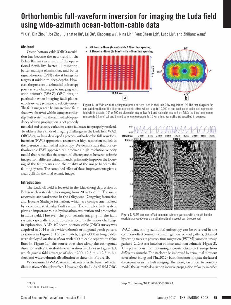
Bohai with water depths ranging from 20 m to 25 m. The main reservoirs are sandstones in the Oligocene Dongying formation and Eocene Shahejie formation, which are compartmentalized by a complex strike-slip fault system. The complex fault system plays an important role in hydrocarbon exploration and production in Luda field. However, the poor seismic imaging for the fault system, especially around reservoir level, is the major challenge in exploration. A 3D-4C ocean-bottom-cable (OBC) survey was acquired in 2014 with a wide-azimuth orthogonal patch pattern as shown in Figure 1. For each patch, eight 6000 m long cables were deployed on the seafloor with 400 m cable separation (blue lines in Figure 1a); the source boat shot along the orthogonal direction with 250 m shot-line separation (red lines in Figure 1a), which gave a fold coverage of about 200, 12.5 m × 12.5 m bin size, and wide-azimuth distribution as shown in Figure 1b.

Wide-azimuth (WAZ) seismic data sets offer the benefit of better illumination of the subsurface. However, for the Luda oil field OBC

Yi Xie1, Bin Zhou2, Joe Zhou1, Jiangtao Hu1, Lei Xu1, Xiaodong Wu1, Nina Lin1, Fong Cheen Loh1, Lubo Liu1, and Zhiliang Wang2

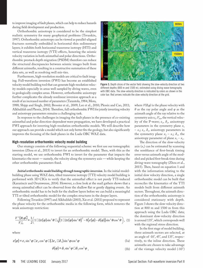
WAZ data, strong azimuthal anisotropy can be observed in the common-offset common-azimuth gathers, or snail gathers, obtained by sorting traces in prestack time migration (PSTM) common-image gathers (CIGs) as a function of offset and then azimuth (Figure 2). This prevents us from obtaining a constructive stack image from different azimuths. The stack can be improved by azimuthal moveout correction (Hung and Yin, 2012), but this cannot mitigate the lateral discrepancies in the fault imaging. Therefore, it is crucial to correctly model the azimuthal variation in wave propagation velocity in order

1CGG.2CNOOC Ltd-Tianjin.

http://dx.doi.org/10.1190/tle36010075.1.

Figure 1. (a) Wide-azimuth orthogonal patch pattern used in the Luda OBC acquisition. (b) The rose diagram for one patch (radius of the diagram represents offset which is up to 10,000 m and each color-coded cell represents fold within a sector 10° × 500 m: blue color means low fold and red color means high fold); the blue inner circle represents 5 km offset and the red outer circle represents 10 km offset. Azimuths are specified in degrees.

Figure 2. PSTM common-offset common-azimuth gathers with azimuth header overlaid above: obvious azimuthal residual moveout can be observed.

Special Section: Full-waveform inversion Part II76 THE LEADING EDGE January 2017

to improve imaging of fault planes, which can help to reduce hazards during field development and production.

Orthorhombic anisotropy is considered to be the simplest realistic symmetry for many geophysical problems (Tsvankin, 1997). Orthorhombic anisotropy can be viewed as parallel-aligned fractures normally embedded in horizontal thin sedimentary layers; it exhibits both horizontal transverse isotropy (HTI) and vertical transverse isotropy (VTI) effects, honoring the seismic velocity variation in both azimuthal and polar directions. Ortho-rhombic prestack depth migration (PSDM) therefore can reduce the structural discrepancies between seismic images built from different azimuths, resulting in a constructive summation of these data sets, as well as resolving well mis-ties.

Furthermore, high-resolution models are critical to fault imag-ing. Full-waveform inversion (FWI) has become an established velocity model building tool that can generate high-resolution veloc-ity models especially in areas well sampled by diving waves, even in geologically complex areas. However, orthorhombic anisotropy further complicates the already nonlinear inversion approach as a result of an increased number of parameters (Tarantola, 1984; Mora, 1988; Shipp and Singh, 2002; Brossier et al., 2009; Lee et al., 2010; Plessix and Cao, 2011; Alkhalifah and Plessix, 2014). Therefore, full orthorhombic FWI for jointly inverting velocity and anisotropy parameters remains a challenging task.

In response to the challenges in imaging the fault planes in the presence of co-existing azimuthal and polar direction-dependent wave propagation, we have developed a practical FWI approach for inverting high-resolution orthorhombic models. We will describe how our approach can provide a model which not only better fits the geology, but also significantly improves the focusing of the fault planes in the Luda OBC WAZ data.

High-resolution orthorhombic velocity model buildingOur strategy consists of the following sequential scheme: we first use our tomographic

inversion (Zhou et al., 2015) to invert for an orthorhombic model. Then, with this as the starting model, we use orthorhombic FWI to invert for the parameter that impacts the kinematics the most — namely, the velocity along the symmetry axis — while keeping the other orthorhombic parameters fixed.

Initial orthorhombic model building through tomographic inversion. In the initial model-building phase using WAZ data, tilted transverse isotropy (TTI) velocity model building is performed with 3D CIGs to verify that the azimuthal effect is not purely TTI-induced (Karazincir and Orumwense, 2014). However, a close look at the snail gathers shows that a strong azimuthal effect can be observed from the shallow flat or gently dipping events. An orthorhombic model has to be built for the shallow layers before we can build a meaningful TTI or tilted orthorhombic model for the complex structures in the deeper layers.

Following Tsvankin (1997) and Alkhalifah (2003), Xie et al. (2011) proposed to represent the phase velocity for the orthorhombic media in the following form, which removes the weak anisotropy restriction:

V 2 θ ,ϕ( )VP 0

2 = 12

1+ 2ε ϕ( )sin 2θ + 1+ 2ε ϕ( )sin 2θ( )2 −8 ε ϕ( )−δ ϕ( )( )sin 2θ cos 2θ⎛⎝

⎞⎠ , (1)

where

ε ϕ( ) = ε 1 sin 4ϕ + ε 2 cos4ϕ + 2ε 2 +δ 3( )sin 2ϕ cos 2ϕ (1a)

δ ϕ( ) = δ 1 sin 2ϕ +δ 2 cos 2ϕ , (1b)

where V(θ,φ) is the phase velocity with θ as the ray polar angle and φ as the azimuth angle of the ray relative to the symmetry axis x1; VP0, the vertical veloc-ity of the P-wave; ε2, δ2, anisotropy parameters in the symmetry plane x1 – x3; ε1, δ1, anisotropy parameters in the symmetry plane x2 – x3; δ3, the anisotropy parameter of plane x1 – x2.

The direction of the slow-velocity axis (x1) can be estimated by scanning the semblance of first-break timing error versus azimuth angle of the mod-eled and picked first-break time during diving-wave tomography (Zhou et al., 2015). Then, based on equation 1 and with the information relating to the initial slow velocity direction, a single orthorhombic model can be built that reconciles the kinematics of the TTI models built from different azimuth sectors. Throughout, the azimuth direc-tion of the orthorhombic anisotropy is considered stationary with depth. Figure 3 shows the slow-velocity direc-tion at 800 m and 1500 m from this approach using the Luda OBC data; the dominant slow-velocity direction is around 135°, which corresponds well with the regional stress direction.

In the first stage of model building, three azimuth sectors are selected, at an angle of -10°, 45°, and 135°, respec-tively, to the inline direction. These azimuths are chosen to take advantage of the vintage velocity model (-10°)

Figure 3. Depth slices of the vector field showing the slow-velocity direction at two different depths (800 m and 1500 m), estimated using diving-wave tomography with OBC data. The slow-velocity direction is indicated by colors as shown in the color bar. Red arrows indicate the slow-velocity direction at the grid.

Special Section: Full-waveform inversion Part II January 2017 THE LEADING EDGE 77

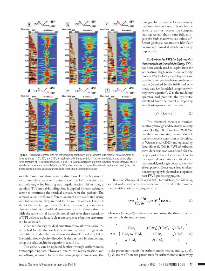
and the dominant slow-velocity direction. For each azimuth sector, we select traces with azimuths within 15° of the nominal azimuth angle for binning and regularization. After that, a standard TTI model-building flow is applied for each azimuth sector to minimize the residual curvature in the gathers. The vertical velocities from different azimuths are calibrated using well log to ensure they are tied to the well velocities. Figure 4 shows the CIGs together with the corresponding semblance plot associated with residual curvature from all three azimuths with the same initial isotropic model and after three iterations of TTI velocity update. A clear convergence of gather curvature can be observed.

Once satisfactory residual curvature from all three azimuths is reached for the shallow layers, we use equation 1 to generate the initial orthorhombic model from the three TTI velocity fields. The initial slow-velocity direction is then refined by data fitting, using the relationship in equations 1a and 1b.

The velocity can be updated further through orthorhombic tomographic update. However, due to the regularization and smoothing required for a stable tomographic inversion, the

tomographic inverted velocity normally has limited resolution to fully resolve the velocity contrast across the complex faulting system, thus it can’t fully miti-gate the fault shadow issues unless suf-ficient geologic constraints like fault horizons are provided, which is normally impractical.

Orthorhombic FWI for high-resolu-tion orthorhombic model building. FWI has been widely used in exploration for generating high-resolution velocity models. FWI velocity model updates are based on a comparison between observed data d (acquired in the field) and syn-thetic data Lm (modeled using the two-way wave equation), L is the modeling operator and predicts the synthetic wavefield from the model m, typically via a least-squares cost function.

f = Lm – d2. (2)

This mismatch then is minimized iteratively through updates to the velocity model (Lailly, 1983; Tarantola, 1984). We use the time domain, preconditioned, steepest-descent algorithm as described in Warner et al. (2013) and updated by Ratcliffe et al. (2014). FWI of reflected wave data was not considered for the deeper part of the velocity model due to the expected uncertainties in the deeper macromodel, making it potentially unreli-able at present. However, a deeper reflec-tion tomography is planned as a separate, post-FWI, processing project.

Based on Zhang and Zhang’s (2011) formulation, the following second-order wave equation is derived in tilted orthorhombic media with spatially varying density:

Lσ = 1VP 0

2∂ 2σ∂t 2 − ρNDT 1

ρDσ = s, (3)

where σ = (σ1, σ2, σ3)T is the vector composing the three principal stresses, s is the source term,

N =

1+ 2ε 2 1+ 2ε 2( ) 1+ 2δ 3 1+ 2δ 2

1+ 2ε 2( ) 1+ 2δ 3 1+ 2ε 1 1+ 2δ 1

1+ 2δ 2 1+ 2δ 1 1

⎡

⎣

⎢⎢⎢⎢

⎤

⎦

⎥⎥⎥⎥

(4)

is the parameter matrix for orthorhombic media, and ε1, ε2, δ1, δ2, δ3 are the Thomsen parameters for orthorhombic anisotropy

Figure 4. PSDM CIGs together with the corresponding semblance plot associated with residual curvature from all three azimuths (-10°, 45°, and 135°, respectively) with the same initial isotropic model (a, b, and c) and after three iterations of TTI velocity update (d, e, and f): a clear convergence of gather curvature can be observed. The TTI model of each azimuth sector flattens the CIG gather from the corresponding azimuth sector pretty well (blue color means low semblance values while red color means high semblance values).

Special Section: Full-waveform inversion Part II78 THE LEADING EDGE January 2017

(Tsvankin, 1997). Two Euler angles, (ϕ, ϑ), are used to define the azimuthal and polar angles of the axis tilted from vertical at each spatial point, as for the symmetry axis in a TTI model. For tilted orthorhombic anisotropy, a third angle β is introduced to rotate the elastic tensor in the local x-y plane and to represent the slow-velocity direction inside this plane.

D = diag R 1T∇,R 2

T∇,R 3T∇( ) is the tilted first-order derivative and Ri

T are column vectors of R, the transformation matrix:

cosφ − sinφ 0sinφ cosφ 00 0 1

⎛

⎝

⎜⎜⎜

⎞

⎠

⎟⎟⎟

cosϑ 0 sinϑ0 1 0

− sinϑ 0 cosϑ

⎛

⎝

⎜⎜⎜

⎞

⎠

⎟⎟⎟

cosβ − sinβ 0sinβ cosβ 00 0 1

⎛

⎝

⎜⎜⎜

⎞

⎠

⎟⎟⎟

. (5)

Finally, VP0 is the velocity along the symmetry axis, ρ is the density, and β is the rotation angle in the local plane.

In the adjoint-state method, com-putation of the gradient of the objective function requires computation of

∂L∂mk

σ⎡⎣⎢

⎤⎦⎥

T

σ b , (6)

where σb is the back-propagated residual wavefield, and the first factor is obtained by solving the wave equation Lσ = s, where s is the source term. The variable mk in the partial derivative represents the parameter we would like to update. Hence, a VP0 update results in

∂L∂VP 0

σ = − 2VP 0

3∂ 2σ∂t 2 . (7)

A joint inversion of velocity and anisotropic field is tempting, however it remains very challenging due to crosstalk between the parameters. We propose a practical approach here: long-wavelength update for the anisotropic parameters while full-wavelength up-date for the velocity because it has first-order impact on kinematics. The aniso-tropic parameters such as ε1 and ε2 were mostly updated by tomographic inver-sion and further fine-tuned by maximiz-ing the cross-correlation coefficient between the modeled and the recorded data as the cost function. The goal here is to make sure the mismatch is not azimuthal related or in a way the ortho-rhombic wavefront is sufficiently hon-ored although the anisotropic param-eters are relatively smooth. This will allow all data from WAZ OBC survey to be used in orthorhombic FWI for high resolution VP0 inversion without worrying about the discrepancy from different azimuth.

ResultsWe apply this flow to the Luda

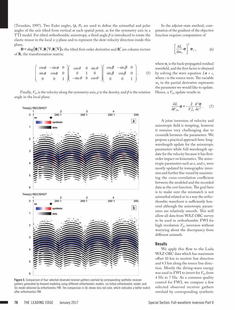
WAZ OBC data which has maximum offset 10 km in receiver line direction and 4.5 km along the source line direc-tion. Mostly the diving-wave energy was used in FWI to invert for VP0 from 4 Hz to 7 Hz. As a common quality control for FWI, we compare a few selected observed receiver gathers overlaid by corresponding synthetic

Figure 5. Comparison of four selected observed receiver gathers overlaid by corresponding synthetic receiver gathers generated by forward modeling using different orthorhombic models. (a) Initial orthorhombic model, and (b) model obtained by orthorhombic FWI. The comparison in (b) shows less red color, which indicates a better match after orthorhombic FWI.

Special Section: Full-waveform inversion Part II January 2017 THE LEADING EDGE 79

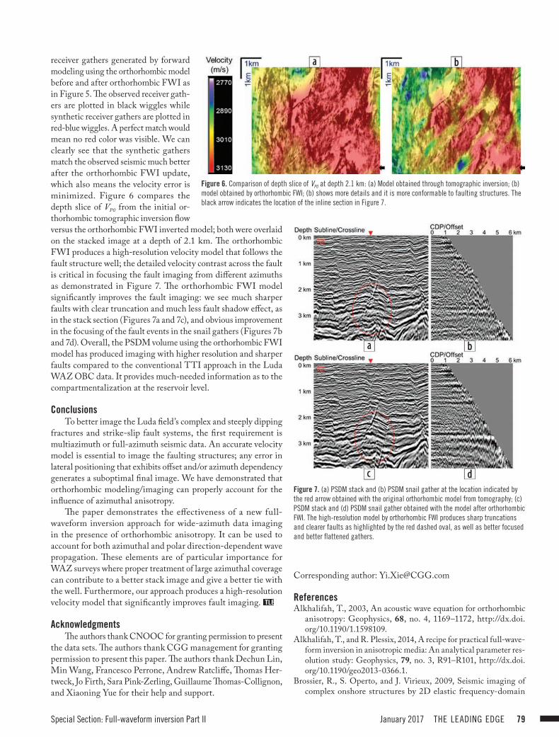
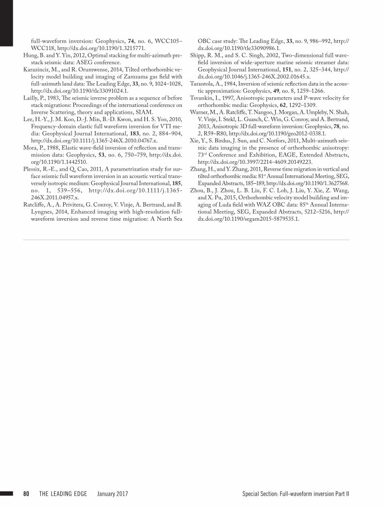
receiver gathers generated by forward modeling using the orthorhombic model before and after orthorhombic FWI as in Figure 5. The observed receiver gath-ers are plotted in black wiggles while synthetic receiver gathers are plotted in red-blue wiggles. A perfect match would mean no red color was visible. We can clearly see that the synthetic gathers match the observed seismic much better after the orthorhombic FWI update, which also means the velocity error is minimized. Figure 6 compares the depth slice of VP0 from the initial or-thorhombic tomographic inversion flow versus the orthorhombic FWI inverted model; both were overlaid on the stacked image at a depth of 2.1 km. The orthorhombic FWI produces a high-resolution velocity model that follows the fault structure well; the detailed velocity contrast across the fault is critical in focusing the fault imaging from different azimuths as demonstrated in Figure 7. The orthorhombic FWI model significantly improves the fault imaging: we see much sharper faults with clear truncation and much less fault shadow effect, as in the stack section (Figures 7a and 7c), and obvious improvement in the focusing of the fault events in the snail gathers (Figures 7b and 7d). Overall, the PSDM volume using the orthorhombic FWI model has produced imaging with higher resolution and sharper faults compared to the conventional TTI approach in the Luda WAZ OBC data. It provides much-needed information as to the compartmentalization at the reservoir level.

ConclusionsTo better image the Luda field’s complex and steeply dipping

fractures and strike-slip fault systems, the first requirement is multiazimuth or full-azimuth seismic data. An accurate velocity model is essential to image the faulting structures; any error in lateral positioning that exhibits offset and/or azimuth dependency generates a suboptimal final image. We have demonstrated that orthorhombic modeling/imaging can properly account for the influence of azimuthal anisotropy.

The paper demonstrates the effectiveness of a new full-waveform inversion approach for wide-azimuth data imaging in the presence of orthorhombic anisotropy. It can be used to account for both azimuthal and polar direction-dependent wave propagation. These elements are of particular importance for WAZ surveys where proper treatment of large azimuthal coverage can contribute to a better stack image and give a better tie with the well. Furthermore, our approach produces a high-resolution velocity model that significantly improves fault imaging.

AcknowledgmentsThe authors thank CNOOC for granting permission to present

the data sets. The authors thank CGG management for granting permission to present this paper. The authors thank Dechun Lin, Min Wang, Francesco Perrone, Andrew Ratcliffe, Thomas Her-tweck, Jo Firth, Sara Pink-Zerling, Guillaume Thomas-Collignon, and Xiaoning Yue for their help and support.

Corresponding author: Yi.Xie@CGG.com

ReferencesAlkhalifah, T., 2003, An acoustic wave equation for orthorhombic

anisotropy: Geophysics, 68, no. 4, 1169–1172, http://dx.doi.org/10.1190/1.1598109.

Alkhalifah, T., and R. Plessix, 2014, A recipe for practical full-wave-form inversion in anisotropic media: An analytical parameter res-olution study: Geophysics, 79, no. 3, R91–R101, http://dx.doi.org/10.1190/geo2013-0366.1.

Brossier, R., S. Operto, and J. Virieux, 2009, Seismic imaging of complex onshore structures by 2D elastic frequency-domain

Figure 6. Comparison of depth slice of VP0 at depth 2.1 km: (a) Model obtained through tomographic inversion; (b) model obtained by orthorhombic FWI; (b) shows more details and it is more conformable to faulting structures. The black arrow indicates the location of the inline section in Figure 7.

Figure 7. (a) PSDM stack and (b) PSDM snail gather at the location indicated by the red arrow obtained with the original orthorhombic model from tomography; (c) PSDM stack and (d) PSDM snail gather obtained with the model after orthorhombic FWI. The high-resolution model by orthorhombic FWI produces sharp truncations and clearer faults as highlighted by the red dashed oval, as well as better focused and better flattened gathers.

Special Section: Full-waveform inversion Part II80 THE LEADING EDGE January 2017

full-waveform inversion: Geophysics, 74, no. 6, WCC105–WCC118, http://dx.doi.org/10.1190/1.3215771.

Hung, B. and Y. Yin, 2012, Optimal stacking for multi-azimuth pre-stack seismic data: ASEG conference.

Karazincir, M., and R. Orumwense, 2014, Tilted orthorhombic ve-locity model building and imaging of Zamzama gas field with full-azimuth land data: The Leading Edge, 33, no. 9, 1024–1028, http://dx.doi.org/10.1190/tle33091024.1.

Lailly, P., 1983, The seismic inverse problem as a sequence of before stack migrations: Proceedings of the international conference on Inverse Scattering, theory and applications, SIAM.

Lee, H.-Y., J. M. Koo, D.-J. Min, B.-D. Kwon, and H. S. Yoo, 2010, Frequency-domain elastic full waveform inversion for VTI me-dia: Geophysical Journal International, 183, no. 2, 884–904, http://dx.doi.org/10.1111/j.1365-246X.2010.04767.x.

Mora, P., 1988, Elastic wave-field inversion of reflection and trans-mission data: Geophysics, 53, no. 6, 750–759, http://dx.doi.org/10.1190/1.1442510.

Plessix, R.-E., and Q. Cao, 2011, A parametrization study for sur-face seismic full waveform inversion in an acoustic vertical trans-versely isotropic medium: Geophysical Journal International, 185, no. 1, 539–556, http://dx.doi.org/10.1111/j.1365-246X.2011.04957.x.

Ratcliffe, A., A. Privitera, G. Conroy, V. Vinje, A. Bertrand, and B. Lyngnes, 2014, Enhanced imaging with high-resolution full-waveform inversion and reverse time migration: A North Sea

OBC case study: The Leading Edge, 33, no. 9, 986–992, http://dx.doi.org/10.1190/tle33090986.1.

Shipp, R. M., and S. C. Singh, 2002, Two-dimensional full wave-field inversion of wide-aperture marine seismic streamer data: Geophysical Journal International, 151, no. 2, 325–344, http://dx.doi.org/10.1046/j.1365-246X.2002.01645.x.

Tarantola, A., 1984, Inversion of seismic reflection data in the acous-tic approximation: Geophysics, 49, no. 8, 1259–1266.

Tsvankin, I., 1997, Anisotropic parameters and P-wave velocity for orthorhombic media: Geophysics, 62, 1292–1309.

Warner, M., A. Ratcliffe, T. Nangoo, J. Morgan, A. Umpleby, N. Shah, V. Vinje, I. Stekl, L. Guasch, C. Win, G. Conroy, and A. Bertrand, 2013, Anisotropic 3D full-waveform inversion: Geophysics, 78, no. 2, R59–R80, http://dx.doi.org/10.1190/geo2012-0338.1.

Xie, Y., S. Birdus, J. Sun, and C. Notfors, 2011, Multi-azimuth seis-mic data imaging in the presence of orthorhombic anisotropy: 73rd Conference and Exhibition, EAGE, Extended Abstracts, http://dx.doi.org/10.3997/2214-4609.20149223.

Zhang, H., and Y. Zhang, 2011, Reverse time migration in vertical and tilted orthorhombic media: 81st Annual International Meeting, SEG, Expanded Abstracts, 185–189, http://dx.doi.org/10.1190/1.3627568.

Zhou, B., J. Zhou, L. B. Liu, F. C. Loh, J. Liu, Y. Xie, Z. Wang, and X. Pu, 2015, Orthorhombic velocity model building and im-aging of Luda field with WAZ OBC data: 85th Annual Interna-tional Meeting, SEG, Expanded Abstracts, 5212–5216, http://dx.doi.org/10.1190/segam2015-5879535.1.