CWP-934

Bayesian approach to facies-constrained waveform inversionfor VTI media

Sagar Singh1, Ilya Tsvankin1 & Ehsan Zahibi Naeini21Center for Wave Phenomena, Colorado School of Mines2 Ikon Science, UK

ABSTRACTHigh-resolution velocity models generated by full-waveform inversion (FWI) can beeffectively used in seismic reservoir characterization. However, FWI in anisotropicelastic media is hampered by the nonlinearity of inversion and parameter trade-offs.Here, we propose a robust way to constrain the inversion workflow using per-faciesrock-physics relationships derived from borehole information (well logs). A proba-bilistic approach in the Bayesian domain is used to create the spatial distribution ofthis prior information and constrain the model updating at each iteration of FWI. Theadvantages of the facies-based FWI are demonstrated on 2D and 3D VTI (transverselyisotropic with a vertical symmetry axis) elastic models with substantial structural com-plexity. In particular, the tests show that our algorithm improves the spatial resolutionof the medium parameters without using ultra-low-frequency data required by conven-tional FWI.

Key words: Full-waveform inversion, Bayesian algorithm, VTI model, geologic fa-cies, rock-physics constraints, well logs, elastic media.

1 INTRODUCTION

Full-waveform inversion (FWI) has been successfully appliedto isotropic and anisotropic acoustic media (Biondi and Al-momin, 2014, Wang and Tsvankin, 2018). However, exten-sion of FWI to more realistic physical models (e.g., elasticand anisotropic) involves serious complications, such as in-creased computational cost and trade-offs between the modelparameters (Plessix and Cao, 2011; Kohn et al., 2012; Wu andAlkhalifah, 2016). The advent of computational technologymakes application of FWI to such models feasible (Warner etal., 2013; Marjanovic et al., 2018; Kamath et al., 2016) but pa-rameter trade-offs and loss of spatial resolution impair the in-version results (Guasch et al., 2012; Vigh et al., 2014, Kamathand Tsvankin, 2016). Also, ultra-low frequencies required byFWI to avoid cycle-skipping can seldom be recorded in sur-face seismic surveys. As a result, FWI often fails to convergeif the initial model does not lie in the “basin of convergence”near the global minimum.

These limitations of conventional FWI can be partiallyovercome using several existing techniques. Common ap-proaches to reducing the inversion nonlinearity include gradi-ent preconditioning or regularization (Tikhonov and Arsenin,1977; Guitton et al., 2011; Loris et al., 2010). These techniquesstabilize the inversion workflow but they require an accurateinitial model and the regularized objective function has to op-erate with smoothed data. Another option to reduce parameter

trade-offs and improve spatial resolution is to use prior infor-mation about the subsurface as a constraint in model updating(e.g., Guitton, 2012; Asnaashari et al., 2013). Although suchprior information can be obtained from well logs, the sparse-ness of borehole locations makes it difficult to account for re-alistic lateral heterogeneity.

Kemper and Gunning (2014) and Zabihi Naeini andExley (2017) propose a framework for AVO (amplitude-variation-with-offset) analysis which employs rock-physicsrelationships for each facies in the model to increase the accu-racy of parameter estimation. A similar methodology for FWI,presented by Kamath et al. (2017) and Zhang et al. (2018), hasproduced promising results (Zhang et al., 2017; Singh et al.,2018). However, because Kamath et al. (2017) incorporate in-formation from a single borehole, an incorrect facies could beassigned to certain grid points if the model were structurallycomplicated with pronounced lateral gradients. The same is-sue produces artifacts (e.g., edge effects) in the inversion re-sults of Zhang et al. (2017, 2018). Singh et al. (2018) pro-pose an image-guided interpolation technique to build a priorconfidence model that accounts for lateral heterogeneity. ABayesian framework is then used to update the confidencemodel at each iteration. The results of Singh et al. (2018) showthat facies-based constraints can guide FWI towards the globalminimum even if the initial model is substantially distorted.

Further improvement in the resolution of the inverted

2 Singh et al.

elastic parameters can be achieved by incorporating con-straints that include all available facies. These facies (e.g.,shale, sand, sandstone, salt, etc.) can be identified at boreholelocations from rock-physics relationships for the elastic pa-rameters. Here, we develop an FWI algorithm that employs aprobabilistic approach in the Bayesian domain designed to uti-lize sparse well-log information. The facies-based constraintsare obtained with a maximum posterior probability technique.

We start by describing the conventional FWI workflowfor elastic VTI media and discuss the main issues that causedeterioration of the inversion results. Then we outline an effi-cient approach to constructing facies-based model constraintsfrom available rock-physics relationships. The algorithm is ap-plied to the 2D Marmousi model and a 3D medium with pro-nounced lateral heterogeneity (both models have VTI sym-metry). Comparison with conventional (unconstrained) FWIdemonstrates that facies-based constraints help increase pa-rameter resolution even when the data do not include ultra-lowfrequencies (0-2 Hz).

2 ELASTIC FULL WAVEFORM INVERSION FORVTI MEDIA

Conventional FWI operates with the least-squares objectivefunction Ed(m) designed to minimize the misfit between thesimulated and observed seismic data:

Ed(m) = ||Wd (dsim−dobs)||2, (1)

where dobs denotes the recorded (here, multicomponent) data,dsim is the data simulated for a trial model, and Wd is a data-weighting operator designed to make the function dimension-less.

Multiparameter inversion increases the nonlinearity ofthe inverse problem and could produce a number of modelsthat explain the observed data. Therefore, the initial model hasto lie in the immediate vicinity (basin of convergence) of theglobal minimum of the objective function. Then the inversioncan be implemented via an efficient local gradient-based ap-proach:

mi+1 = mi +αi Pi, (2)

where mi is the model-parameter vector at the ith iteration, αiis the step length, and Pi is the direction of the model updating.To model multicomponent seismic data for VTI media, we usethe elastic wave equation:

ρ∂2ui

∂t2 =∂

∂x j

(ci jkl

∂uk

∂xl

)+Fi, (3)

where u is the displacement field, ρ is the density, F is thedensity of the body forces, and ci jkl(i, j,k, l = 1,2,3) are thestiffness coefficients; summation over repeated indices is im-plied. The gradient of the objective function with respect to the

model parameters is obtained from the adjoint-state method(Plessix, 2006; Kamath and Tsvankin, 2016):

∂Ed(m)

∂m=−

[∂dsim

∂m

]WT

d Wd(dobs−dsim); (4)

the subscript “T ” denotes the transpose.The relationships between the stiffness coefficients and

VTI parameters as well as exact expressions for the FWI gra-dient can be found in Appendix A. For the numerical exam-ples below, iterative parameter updating is carried out with amultiscale approach using the nonlinear conjugate-gradient al-gorithm (e.g., Hager and Zhang, 2006).

3 FACIES-BASED CONSTRAINTS IN BAYESIANDOMAIN

We supplement the conventional data-fitting objective functionEd(m) in equation 1 with facies-based constraints as follows:

E(m) = Ed(m)+β E f (m); (5)

E f (m) = ||Wm (minv−mf)||2. (6)

Here Wm is a weighting operator designed to make thefacies-based term dimensionless, the vector mf represents thefacies-based constraints, minv is the inverted model, and β isa scaling factor. The prior rock-physics constraints in the termE f (m) are supposed to be based on the available geologic fa-cies.

The facies-based term is similar to that in Singh et al.(2018), where the initial constraints are obtained from image-guided interpolation. Here, the facies-based model is a func-tion of the inverted model parameters and prior knowledge ofthe facies [i.e., mf ≡ f (minv, f) , where f represents the faciesvector].

In general, interpolation or extrapolation of sparse well-log data cannot properly account for lateral heterogeneity. Tocreate the spatial distribution of a model parameter based onprior information from available well logs, we use a proba-bilistic Bayesian approach that employs information about fa-cies. The FWI workflow is constrained by rock-physics rela-tionships for each individual facies. The depth trends obtainedfrom the well logs are used to compute the posterior probabil-ity of a facies:

Ppost = k[P(f) ·P(m|f)

], (7)

where P(f) is the picking probability of the facies (equal toprior probability of the facies vector f), P(m|f) is the likeli-hood function defined below, k is a scaling coefficient (the sumof the posterior probabilities for all facies), and m representsthe model obtained by the conventional FWI.

The uncertainty in the model space is described by aGaussian distribution (Tarantola, 1984):

Facies-based FWI 3

P(m|f) = 1√2πσ2

i

exp[−

(m− f mi ) · (m− f m

i )

2σ2i

], (8)

where f mi is the mean and σi is the variance of the depth trend

of the ith facies (fi).The posterior probability is computed from equation 7

for each facies at all grid points of the model. The facies withthe maximum posterior probability at a certain grid point isthen compared with the corresponding depth trend. The valuein that depth trend that best matches the current grid-pointvalue of the inverted model parameter (minv

i ) is then assignedto the facies-based model (m f ) at that grid point. Because thatmodel depends on the inverted parameters at each iteration,the facies-based updates are influenced by the inversion re-sults. Therefore, we refer to these constraints as “facies-basedmodels.” In addition to the estimated parameters, the algorithmproduces the final facies-based models (mf), which could bedirectly used in reservoir characterization.

4 SYNTHETIC EXAMPLES

We test the proposed methodology on 2D and 3D elasticVTI models. The elastic wave equation 3 is solved using afourth-order finite-difference algorithm on a staggered gridwith CPML (convolutional perfectly matched layers) bound-ary conditions on the sides of the model.

4.1 2D VTI Marmousi model

First, we carry out FWI for a modified 2D elastic Marmousimodel (Martin et al., 2006). The medium is parameterized bythe P- and S-wave vertical velocities (VP0 and VS0) and theP-wave horizontal and normal-moveout velocities (Vhor,P andVnmo,P). These four parameters control the signatures of thein-plane polarized P- and SV-waves. The horizontal and NMOvelocities are expressed through the Thomsen parameters ε

and δ as follows:

Vhor,P =VP0√

1+2ε ,

Vnmo,P =VP0√

1+2δ .

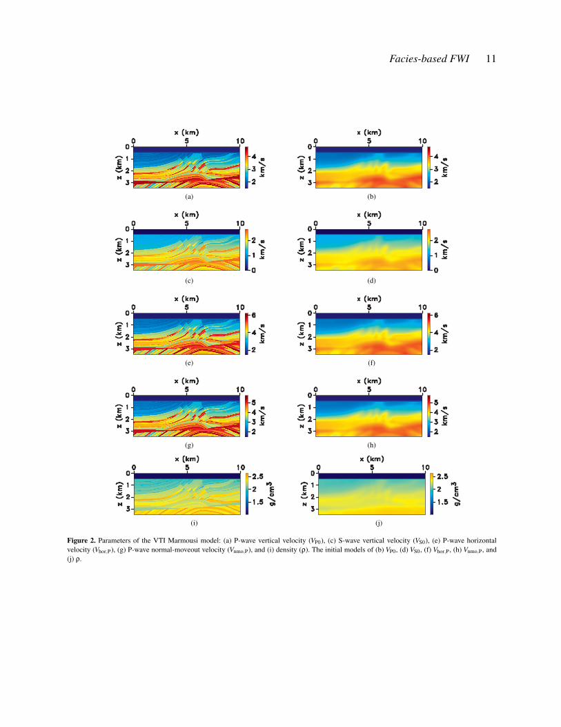
For our version of the Marmousi model, we define theanisotropy coefficients through density as follows: ε= 0.25ρ−0.3 and δ = 0.125ρ−0.1 (Duan and Sava, 2016). The sectionis overlaid by a 460 m-thick water layer (Figure 2 (a), (c), (e),(g), and (i)). Multicomponent data (the vertical and horizon-tal displacements) are generated by 100 shots and recorded by400 receivers evenly distributed along the line and placed 40 mand 460 m, respectively, beneath the surface. The source rep-resents a point explosion; the source signal is a Ricker waveletwith a central frequency of 10 Hz.

The source wavelet and recorded data are filtered (cor-responding to the selected frequency range, see below) prior

to inversion. To compensate for amplitude decay due to geo-metric spreading, the gradients are preconditioned using theapproach of Plessix and Mulder (2004). Therefore, the ele-ments of Wd in equation 1 are equal to unity (the units ofWd are 1/dim(d)). The algorithm is designed to invert for allfive pertinent medium parameters (VP0, VS0, Vhor,P, Vnmo,P, andρ) simultaneously using the inversion gradients listed in Ap-pendix A.

The low frequencies in the 0-2 Hz range, which can sel-dom be acquired in the field, are filtered out from the observeddata. The initial parameters (Figure 2(b), (d), (f), (h), and (j))are obtained by smoothing the actual models, which preservesthe long-wavelength parameter components. Figure 3 displaysvertical profiles that illustrate the deviations of the initial pa-rameters from the actual values. The output of FWI withoutfacies-based constraints is shown in Figure 4(a), (c), (e), (g),and (i); the inversion was performed for all shots in four fre-quency bands (2–5 Hz, 2–8 Hz, 2–13 Hz, 2–19 Hz). Whereasthe estimates of the vertical velocities VP0 and VS0 and the hor-izontal velocity Vhor,P are sufficiently accurate in the shallowpart of the section (the results deteriorate with depth), the ve-locity Vnmo,P and density are strongly distorted due to param-eter trade-offs and the absence of low frequencies (Figure 5).

To determine whether facies information can overcomethese issues, we apply our algorithm with the same frequencybands. The rock-physics constraints for the inversion work-flow are computed from well data at two locations (Figure 6).To obtain the facies distribution, we employ the rock-physicsrelationships for the original isotropic Marmousi model (Table1). After extracting the part of well-log data corresponding to aparticular facies (Figure 6), we compute the mean and varianceof that facies. Although the accuracy of these values wouldincrease if more well logs were available, even sparse priorinformation improves the convergence of the objective func-tion. The facies-based constraints are obtained without explic-itly using the locations of the available wells. At each iteration,the algorithm is implemented as follows:

• Compute the depth trends based on the available rock-physics relationships (Table 1).• Compute the facies-likelihood probability from equation

8. The picking probability is considered 0.25 in our case. How-ever, a more robust approach such as the Markov chain randommodel could provide more reliable picking-probability values.• Compute the posterior probability (equation 7) at each

grid point for each facies.• After determining the facies corresponding to the max-

imum posterior probability, find the value in the depth trendthat best matches the parameter value at each grid point in theinverted model.• Assign the value in the depth trend to the facies-based

model.• Repeat the process for the next iteration.

As mentioned above, the model-weighting vector (Wm)is designed to compensate for geometric spreading. This ap-proach is similar to that in Asnaashari et at. (2013), where theoperator WT

m Wm is scaled by 1/z2, where z is depth. In our

4 Singh et al.

facies ( f ) VP (m/s) VS (m/s) ρ (g/cm3)

water 1500 0 1.01

sand VP VS = 0.804VP−856 ρ = 0.2736V 0.261P

shale VP VS = 0.770VP−867 ρ = 0.2806V 0.265P

marl VP VS = 1.017∗10−3VP−0.055∗10−6V 2P −1.03 ρ = 0.2736V 0.261

P

salt 4500 2600 2.14

Table 1. Isotropic rock-physics relationships for each facies present in the Marmousi model (adapted from Martin et al., 2006). VP represents thespatially varying P-wave velocity (same as VP0 in Figure 2(a)).

implementation, the facies-based term in equation 1 is scaledby the factor β. At each iteration, β can be adjusted to im-prove convergence toward the actual model. Such adjustmentfor field-data applications should depend on the accuracy ofthe prior model and data quality.

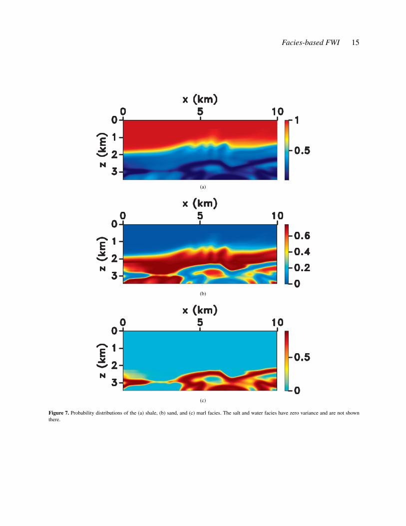
The posterior probability of the facies present in the ini-tial model (Figure 7) is used to build the initial facies-basedconstraints (Figure 8(a), (c), (e), (g), and (i)) by employing theBayesian framework discussed earlier. The facies-based algo-rithm reconstructs the model parameters with much higher ac-curacy (Figures 4(b), (d), (f), (h), (j)) than the conventionalFWI (Figure 5). In particular, note the improved spatial res-olution in the NMO velocity Vnmo,P. The final facies-basedconstraints (Figure 8(b), (d), (f), (h), (j)) closely match theactual models, which means that the inversion was properlyconstrained. It is clear from Figure 9 that the implementedfacies-based constraints efficiently guide the inversion towardthe global minimum of the objective function.

4.2 3D VTI model

The proposed facies-constrained technique is extended to 3DVTI media parameterized by the velocities VP0, VS0, Vhor,P,Vnmo,P, and Vhor,SH (Kamath and Tsvankin, 2016), where

Vhor,SH = VS0√

1+2γ

is the horizontal velocity of SH-waves and γ is Thomsen’sanisotropy parameter. Laboratory studies suggest that thevalue of γ for many rock formations (mostly shales) is closeto ε (Wang, 2002), so Vhor,SH in our model is obtained by set-ting γ = ε.

Here, we present the results of an initial test for a 3D elas-tic VTI medium that contains small blocks (heterogeneities)in the middle of the model (Figure 10). To simulate the wave-field, a time-domain 3D isotropic elastic finite-difference mod-eling code SOFI3D (Bohlen, 2002) was extended to VTI me-dia. Synthetic data are generated for twelve sources and 169receivers, which are evenly distributed over horizontal planes

at depths of 40 and 200 m, respectively (Figure 10). The initialmodels represent smoothed versions of the actual 3D parame-ter distributions that preserve the long-wavelength model com-ponents (Figure 11(b), (d), (f) and 12(b), (d), (f)). The smooth-ing is carried out using a Gaussian smoothing radius of 50 inall directions. The inversion gradient expressions for 3D VTImodels are presented in Appendix A. To optimize the memoryusage, the gradients are recomputed for every third time stepin the time loop (see equation 9 in Appendix A).

The conventional 3D FWI algorithm is applied with themultiscale approach in four frequency bands (2-5 Hz, 2-10Hz, 2-15 Hz, 2-20 Hz). In the absence of model constraints,the inversion does not produce noticeable improvements in theparameter resolution, and the velocity fields are strongly dis-torted (Figure 13(a), (c), (e) and 14(a), (c), (e)).

Next, we employ facies-based constraints derived fromjust four well logs without assuming that the correspondingborehole locations are known. Because the model is relativelysimple, we do not use the maximum posterior probability tech-nique. Instead, different values obtained from well logs aretreated as an individual facies. The closest match between eachinverted parameter and a certain facies at each grid point yieldsthe facies-based constraints. The constrained FWI algorithmsubstantially improves the spatial resolution of the inverted pa-rameters and clearly outperforms the conventional FWI (Fig-ure 13(b), (d), (f) and 14(b), (d), (f)).

5 CONCLUSIONS

We proposed a Bayesian framework designed to incorporateprior information about the subsurface facies into the FWIworkflow. Rock-physics descriptions of different facies aresupposed to be obtained from well logs. Because borehole lo-cations are generally sparse, a spatial distribution of facies-based constraints is created by a probabilistic approach inthe Bayesian domain by employing rock-physics relationships.These constraints reduce the nonlinearity of FWI and help inguiding the inversion toward the global minimum of the ob-jective function.

Facies-based FWI 5

In contrast to the conventional FWI that has to rely onultra-low frequencies, the lower bound of the frequency rangeused in our examples is limited by 2 Hz. Synthetic tests for2D and 3D VTI models confirm the significant advantagesof the facies-based FWI over conventional waveform inver-sion. Our algorithm was able to mitigate parameter trade-offsthat hamper the conventional inversion for anisotropic mediaand to produce high-resolution models despite the absence ofthe ultra-low frequencies in the data. Furthermore, the facies-based models generated by our algorithm can provide valuableinformation about reservoir properties.

6 ACKNOWLEDGMENTS

We thank the members of the A(anisotropy)-Team at the Cen-ter for Wave Phenomena (CWP) for useful discussions. Thiswork was supported by the Consortium Project on SeismicInverse Methods for Complex Structures at the Center forWave Phenomena (CWP) and competitive research fundingfrom the King Abdullah University of Science and Technol-ogy (KAUST).

REFERENCES

Asnaashari, A., R. Brossier, S. Garambois, F. Audebert, P.Thore, and J. Virieux, 2013, Regularized seismic full wave-form inversion with prior model information: Geophysics,78, no. 2, R25–R36, doi: 10.1190/GEO2012-0104.1.

Biondi, B., and A. Almomin, 2014, Efficient and ro-bust waveform-inversion workflow: 84th Annual Interna-tional Meeting, SEG, Expanded Abstracts, 917–921, doi:10.1190/segam2014-1475.1.

Bohlen, T. 2002, Parallel 3-D viscoelastic finite-differenceSeismic Modelling: Computers and Geosciences, 28, no. 8,887-899, doi: 10.1016/S0098-3004(02)00006-7.

Bunks, C., F. Saleck, S. Zaleski, and G. Chavent, 1995,Multiscale seismic waveform inversion: Geophysics, 60,1457–1473, doi: 10.1190/1.1443880.

Duan, Y. and P. Sava, 2016, Elastic wavefield tomographywith physical model constraints: Geophysics, 81, no. 6,R447-R456, doi: 10.1190/GEO2015-0508.1.

Guasch, L., M. Warner, T. Nangoo, J. Morgan, A. Umpleby, I.Stekl, and Shah, N., 2012, Elastic 3D full-waveform inver-sion: 82nd Annual International Meeting, SEG, ExpandedAbstracts, doi: 10.1190/segam2012-1239.1.

Guitton, A., G. Ayeni, and E. Daz, 2012, Constrained full-waveform inversion by model reparameterization: Geo-physics, 77, no. 2, R117–R127, doi: 10.1190/geo2011-0196.1.

Guitton, A., 2011, A blocky regularization scheme forfull waveform inversion: 81st Annual InternationalMeeting, SEG, Expanded Abstracts, 2418–2422, doi:10.1190/1.3627694.

Hager, W. W., and H. Zhang 2006, A survey of nonlinear con-jugate gradient methods: Pacific Journal of Optimization, 6,no. 2, 35-58.

Kamath, N., and I. Tsvankin, 2016, Elastic full-waveforminversion for VTI media: Methodology and sensitiv-ity analysis: Geophysics, 81, no. 2, C53–C68, doi:10.1190/geo2014-0586.1.

Kamath, N., I. Tsvankin, and E. Diaz, 2017, Elastic full-waveform inversion for VTI media: A synthetic parame-terization study: Geophysics, 82, no. 5, C163-C174, doi:10.1190/GEO2016-0375.1.

Kamath, N., I. Tsvankin, and E. Zabihi Naeini, 2017, Facies-constrained FWI: Toward application to reservoir charac-terization: The Leading Edge, 36, no. 11, 924-930, doi:10.1190/tle36110924.1.

Kemper, M., and J. Gunning, 2014, Joint impedance and fa-cies inversion–seismic inversion redefined: First Break, 32,no. 9, 89-95.

Kohn, D., D. De Nil, A. Kurzmann, A. Przebindowska, andT. Bohlen, 2012, On the influence of model parametrizationin elastic full waveform tomography: Geophysical Jour-nal International, 191, no. 1, 325-345, doi: 10.1111/j.1365-246X.2012.05633.x.

Loris, I., H. Douma, G. Nolet, I. Daubechies, and C. Re-gone, 2010, Nonlinear regularization techniques for seis-mic tomography: Journal of Computational Physics, 229,890–905, doi: 10.1016/j.jcp.2009.10.020.

Martin, G., R. Wiley, and K. J. Marfurt, 2006, Marmousi2:An elastic upgrade for Marmousi: The Leading Edge, 25,no. 2, 156-166, doi: 10.1190/1.2172306.

Marjanovic, M., R.-E Plessix, A. Stopin, and S. C. Singh,2018, Elastic versus acoustic 3-D Full Waveform Inversionat the East Pacific Rise 950N: Geophysical Journal Interna-tional, 216, no. 3, 1497–1506, doi: 10.1093/gji/ggy503.

Plessix, R.-E. and Q. Cao, 2011, A parametrization studyfor surface seismic full waveform inversion in an acousticvertical transversely isotropic medium: Geophysical Jour-nal International, 185, no. 1, 539–556, doi: 10.1111/j.1365-246X.2011.04957.x.

Plessix, R.-E. and W. A. Mulder, 2004, Frequency-domainfinite-difference amplitude-preserving migration: Geophys-ical Journal International, 157, no. 3, 975–987, doi:10.1111/j.1365-246X.2004.02282.x.

Singh, S., I. Tsvankin, and E. Zabihi Naeini, 2018, Bayesianframework for elastic full-waveform inversion with faciesinformation: The Leading Edge, 37, no. 12, 924-931, doi:10.1190/tle37120924.1.

Tarantola, A., 1984, Inversion of seismic reflection data in theacoustic approximation: Geophysics, 49, 1259–1266, doi:10.1190/1.1441754.

Tsvankin, I., 2012, Seismic signature and analysis of reflec-tion data in anisotropic media: 3rd ed., Society of Explo-ration Geophysicists, doi: 10.1190/1.9781560803003.

Tikhonov, A., and V. Arsenin, 1977, Solution of ill-posedproblems: Winston and Sons, 1-258.

Vigh, D., K. Jiao, D. Watts, and D. Sun, 2014, Elasticfull-waveform inversion application using multicomponentmeasurements of seismic data collection: Geophysics, 79,no. 2, R63–R77, doi: 10.1190/geo2013-0055.1.

Wang, Z., 2002, Seismic anisotropy in sedimentary rocks,

6 Singh et al.

part 2: Laboratory data: Geophysics, 67, no. 5, 1423-1440,doi: 10.1190/1.1512743.

Wang, H., and I. Tsvankin, 2018, Methodology of waveforminversion for acoustic orthorhombic media: Journal of Seis-mic Exploration, 27, 201-226.

Warner, M., A. Ratcliffe, T. Nangoo, J. Morgan, A. Umpleby,N. Shah, V. Vinje, I. Stekl, L. Guasch, C. Win, G.Conroy, and A. Bertrand, 2013, Anisotropic 3D full-waveform inversion: Geophysics, 78, no. 2, R59-R80, doi:10.1190/GEO2012-0338.1

Wu, Z. and T. Alkhalifah, 2016, Waveform inversion foracoustic VTI media in frequency domain: 86th SEG Tech-nical Program Expanded Abstracts, SEG, Expanded Ab-stracts, 1184–1189, doi: 10.1190/segam2016-13867221.1.

Yan, J. and P. Sava, 2011, Elastic wave-mode separationfor TTI media: Geophysics, 76, no. 4, T65-T78, doi:10.1190/1.3255781.

Zhang, Z., T. Alkhalifah, and E. Zabihi Naeini, 2017,Multiparameter elastic full waveform Inversion with fa-cies constraints: 87th SEG Technical Program ExpandedAbstracts, SEG, Expanded Abstracts,, 1551-1555, doi:10.1190/segam2017-17672943.1.

Zhang, Z., T. Alkhalifah, E. Zabihi Naeini, and B. Sun, 2018,Multiparameter elastic full waveform inversion with facies-based constraints: Geophysical Journal International, 213,no. 3, 2112-2127, doi: 10.1093/gji/ggy113.

Zabihi Naeini, E., and R. Exley, 2017, Quantitative interpre-tation using facies-based seismic inversion: Interpretation,5, no. 3, 1-8, doi: 10.1190/INT-2016-0178.1.

Zabihi Naeini, E., T. Alkhalifah, I. Tsvankin, N. Kamath, andJ. Cheng, 2016, Main components of full waveform inver-sion for reservoir characterization: First Break, 34, 37-48,doi: 10.3997/1365-2397.2016015.

Facies-based FWI 7

APPENDIX A

3D GRADIENTS FOR FWI INVERSION

Using the two-index Voigt notation, the stiffness matrix for VTI media can be written as (Tsvankin, 2012):C11 C11−2C66 C13 0 0 0

C11−2C66 C11 C13 0 0 0C13 C13 C33 0 0 0

0 0 0 C55 0 00 0 0 0 C55 00 0 0 0 0 C66

Our algorithm operates with the P- and S-wave vertical velocities (VP0 and VS0), P-wave normal-moveout and horizontalvelocities (Vnmo,P and Vhor,P) and SH-wave horizontal velocity (Vhor,SH). The stiffness coefficients are related to these velocities asfollows:

C11 = ρ V 2hor,P ,

C13 = ρ

[√(V 2

P0−V 2S0)(V

2nmo,P−V 2

S0)−V 2S0

],

C33 = ρ V 2P0 ,

C55 = ρ V 2S0 ,

C66 = ρ V 2hor,SH .

The gradient of the FWI data-difference objective function (equation 1) in elastic VTI media is obtained by Kamath et al.(2016) as:

∂Ed

∂mn=−∑

i jkl

(∫ T

0

∂ui

∂x j

∂ψk

∂xl

)∂ci jkl

∂mn, (9)

where i, j,k, l = 1,2,3, T is the total time of wave propagation, u and ψψψ are the forward and back-propagated displacement fields,respectively, and the vector m represents the model parameters (m1 =VP0, m2 =VS0, m3 =Vnmo,P, m4 =Vhor,P, m5 =Vhor,SH, andm6 = ρ).

The gradients for these parameters have the form:

∂Ed

∂VP0=−2ρVP0

∫ T

0

[∂ψz

∂z∂uz

∂z+

q2

(∂ψx

∂x∂uz

∂z+

∂ψz

∂z∂ux

∂x+

∂ψy

∂y∂uz

∂z+

∂ψz

∂z∂uy

∂y

)]dt , (10)

∂Ed

∂VS0= 2ρVS0

∫ T

0

{[1+

q2+

12q

](∂ψx

∂x∂uz

∂z+

∂ψz

∂z∂ux

∂x+

∂ψy

∂y∂uz

∂z+

∂ψz

∂z∂uy

∂y

)−(

∂ψx

∂z+

∂ψz

∂x

)(∂ux

∂z+

∂uz

∂x

)−(

∂uy

∂z+

∂uz

∂y

)(∂ψy

∂z+

∂ψz

∂y

)}dt

, (11)

∂Ed

∂Vnmo,P=−ρVnmo,P

q

∫ T

0

(∂ψx

∂x∂uz

∂z+

∂ψz

∂z∂ux

∂x+

∂ψz

∂z∂uy

∂y+

∂ψy

∂y∂uz

∂z

)dt , (12)

∂Ed

∂Vhor,P=−2ρVhor,P

∫ T

0

(∂ψy

∂y+

∂ψx

∂x

)(∂uy

∂y+

∂ux

∂x

)dt , (13)

∂Ed

∂Vhor,SH=−2ρVhor,S

∫ T

0

{(∂ψx

∂y+

∂ψy

∂x

)(∂ux

∂y+

∂uy

∂x

)−2(

∂ux

∂x∂ψy

∂y+

∂uy

∂y∂ψx

∂x

)}dt , (14)

8 Singh et al.

∂Ed

∂ρ=−

∫ T

0

[V 2

P0

(∂uz

∂z∂ψz

∂z

)+V 2

hor,P

(∂ux

∂x∂ψx

∂x+

∂uy

∂y∂ψy

∂y+

∂ux

∂x∂ψy

∂y+

∂uy

∂y∂ψx

∂x

)+

V 2S0

{(∂ψx

∂z+

∂ψz

∂x

)(∂ux

∂z+

∂uz

∂x

)+(

∂ψy

∂z+

∂ψz

∂y

)(∂uy

∂z+

∂uz

∂y

)}+

V 2hor,SH

{(∂ψx

∂y+

∂ψy

∂x

)(∂ux

∂y+

∂uy

∂x

)−2

∂ux

∂x∂ψy

∂y−2

∂uy

∂y∂ψx

∂x

}+(√

(V 2nmo,P−V 2

S0)(V2P0−V 2

S0)−V 2S0

)(∂ux

∂x∂ψz

∂z+

∂uz

∂z∂ψx

∂x+

∂uy

∂y∂ψz

∂z+

∂uz

∂z∂ψy

∂y

)+

vxΨx + vyΨy + vzΨz

]dt ,

(15)

where

q =

√√√√V2nmo,P−V2

S0

V2P0−V2

S0.

Here, vvv and ΨΨΨ are the forward- and back-propagated velocity fields, respectively. The corresponding 2D gradient expressions areobtained by removing the derivatives with respect to the transverse coordinate y.

Facies-based FWI 9

LIST OF FIGURES

Figure 1. Flowchart for reservoir-oriented FWI with facies-based constraints (after Singh et al., 2018, and Zabihi Naeini etal., 2016).

Figure 2. Parameters of the VTI Marmousi model: (a) P-wave vertical velocity (VP0), (c) S-wave vertical velocity (VS0), (e)P-wave horizontal velocity (Vhor,P), (g) P-wave normal-moveout velocity (Vnmo,P), and (i) density (ρ). The initial models of (b)VP0, (d) VS0, (f) Vhor,P, (h) Vnmo,P, and (j) ρ.

Figure 3. Vertical profiles of the P- and S-wave vertical velocities and density at x = 5 km that illustrate the accuracy of theinitial model. The actual parameters are marked by blue lines and the corresponding initial parameters used for FWI are in red. Thevelocities Vhor,P and Vnmo,P are derived from VP0 and ρ and are not shown here.

Figure 4. Results of the conventional FWI for the model in Figure 2: (a) VP0, (c) VS0, (e) Vhor,P, (g) Vnmo,P, and (i) ρ. Theresults of the facies-based FWI: (b) VP0, (d) VS0, (f) Vhor,P, (h) Vnmo,P, and (j) ρ. The frequency range for the inversion is 2–19 Hz.

Figure 5. Vertical profiles of the P-wave NMO velocity and density at x = 5 km: the actual parameters (blue lines) and theresults of the conventional (yellow) and facies-based (red) FWI.

Figure 6. Depth trends for the facies from the well data at (a) x = 3.6 km and (b) x = 4.8 km. The trends are computed fromthe rock-physics relationships in Table 1; the velocities are in km/s.

Figure 7. Probability distributions of the (a) shale, (b) sand, and (c) marl facies. The salt and water facies have zero varianceand are not shown there.

Figure 8. Initial facies-based models for: (a) VP0, (c) VS0, (e) Vhor,P, (g) Vnmo,P, and (i) ρ. The final facies-based models for:(b) VP0, (d) VS0, (f) Vhor,P, (h) Vnmo,P, and (j) ρ.

Figure 9. Normalized objective functions for the conventional and facies-based FWI in the frequency range 2-5 Hz.

Figure 10. Surface acquisition geometry for a 3D VTI model. That data are excited by twelve sources (blue stars) andrecorded by 169 receivers (yellow dots).

Figure 11. Horizontal slices of a 3D VTI model at depth z = 1.5 km: (a) P-wave vertical velocity (VP0), (c) P-wave horizontalvelocity (Vhor,P), and (e) P-wave normal-moveout velocity (Vnmo,P). The initial models of (b) VP0, (d) Vhor,P, and (f) Vnmo,P.

Figure 12. Horizontal slices of the same 3D VTI model as in Figure 10 at depth z = 1.5 km: (a) S-wave vertical velocity(VS0), (c) SH-wave horizontal velocity (Vhor,SH), and (e) density ρ. The initial models of (b) VS0, (d) Vhor,SH, and (f) ρ.

Figure 13. Results of the conventional FWI for the horizontal slice at depth z = 1.5 km: (a) VP0, (c) Vhor,P, and (e) Vnmo,P. Theresults of the facies-based FWI: (b) VP0, (d) Vhor,P, and (f) Vnmo,P.

Figure 14. Results of the conventional FWI for the horizontal slice at depth z = 1.5 km: (a) VS0, (c) Vhor,SH, and (e) ρ. Theresults of the facies-based FWI: (b) VS0, (d) Vhor,SH, and (f) ρ.

10 Singh et al.

Update Forward model

Adjoint

Rock-physicsconstraints

ComparisonSyntheticshot gathers

Recordedshot gathers

Objective Function

Computefacies-basedgradients

Figure 1. Flowchart for reservoir-oriented FWI with facies-based constraints (after Singh et al., 2018, and Zabihi Naeini et al., 2016).

Facies-based FWI 11

(a) (b)

(c) (d)

(e) (f)

(g) (h)

(i) (j)

Figure 2. Parameters of the VTI Marmousi model: (a) P-wave vertical velocity (VP0), (c) S-wave vertical velocity (VS0), (e) P-wave horizontalvelocity (Vhor,P), (g) P-wave normal-moveout velocity (Vnmo,P), and (i) density (ρ). The initial models of (b) VP0, (d) VS0, (f) Vhor,P, (h) Vnmo,P, and(j) ρ.

12 Singh et al.

2 3 4VP0 (km/s)

0.4

1

2

3

z (k

m)

0 1 2VS0 (km/s)

0.4

1

2

3

1 2 3

(g/cm 3)

0.4

1

2

3

Figure 3. Vertical profiles of the P- and S-wave vertical velocities and density at x = 5 km that illustrate the accuracy of the initial model. The actualparameters are marked by blue lines and the corresponding initial parameters used for FWI are in red. The velocities Vhor,P and Vnmo,P are derivedfrom VP0 and ρ and are not shown here.

Facies-based FWI 13

(a) (b)

(c) (d)

(e) (f)

(g) (h)

(i) (j)

Figure 4. Results of the conventional FWI for the model in Figure 2: (a) VP0, (c) VS0, (e) Vhor,P, (g) Vnmo,P, and (i) ρ. The results of the facies-basedFWI: (b) VP0, (d) VS0, (f) Vhor,P, (h) Vnmo,P, and (j) ρ. The frequency range for the inversion is 2–19 Hz.

14 Singh et al.

1 2 3

(g/cm 3)

0.4

1

2

3

2 4 6Vnmo, P (km/s)

0.4

1

2

3

z (k

m)

Figure 5. Vertical profiles of the P-wave NMO velocity and density at x = 5 km: the actual parameters (blue lines) and the results of the conventional(yellow) and facies-based (red) FWI.

(a)

(b)

Figure 6. Depth trends for the facies from the well data at (a) x = 3.6 km and (b) x = 4.8 km. The trends are computed from the rock-physicsrelationships in Table 1; the velocities are in km/s.

Facies-based FWI 15

(a)

(b)

(c)

Figure 7. Probability distributions of the (a) shale, (b) sand, and (c) marl facies. The salt and water facies have zero variance and are not shownthere.

16 Singh et al.

(a) (b)

(c) (d)

(e) (f)

(g) (h)

(i) (j)

Figure 8. Initial facies-based models for: (a) VP0, (c) VS0, (e) Vhor,P, (g) Vnmo,P, and (i) ρ. The final facies-based models for: (b) VP0, (d) VS0, (f)Vhor,P, (h) Vnmo,P, and (j) ρ.

Facies-based FWI 17

0 20 40 60 80 100 120 140Iteration

0

0.2

0.4

0.6

0.8

1ConventionalFacies-based

Figure 9. Normalized objective functions for the conventional and facies-based FWI in the frequency range 2-5 Hz.

Figure 10. Surface acquisition geometry for a 3D VTI model. That data are excited by twelve sources (blue stars) and recorded by 169 receivers(yellow dots).

18 Singh et al.

Figure 11. Horizontal slices of a 3D VTI model at depth z = 1.5 km: (a) P-wave vertical velocity (VP0), (c) P-wave horizontal velocity (Vhor,P), and(e) P-wave normal-moveout velocity (Vnmo,P). The initial models of (b) VP0, (d) Vhor,P, and (f) Vnmo,P.

Facies-based FWI 19

Figure 12. Horizontal slices of the same 3D VTI model as in Figure 10 at depth z = 1.5 km: (a) S-wave vertical velocity (VS0), (c) SH-wavehorizontal velocity (Vhor,SH), and (e) density ρ. The initial models of (b) VS0, (d) Vhor,SH, and (f) ρ.

20 Singh et al.

Figure 13. Results of the conventional FWI for the horizontal slice at depth z = 1.5 km: (a) VP0, (c) Vhor,P, and (e) Vnmo,P. The results of thefacies-based FWI: (b) VP0, (d) Vhor,P, and (f) Vnmo,P.

Facies-based FWI 21

Figure 14. Results of the conventional FWI for the horizontal slice at depth z = 1.5 km: (a) VS0, (c) Vhor,SH, and (e) ρ. The results of the facies-basedFWI: (b) VS0, (d) Vhor,SH, and (f) ρ.