solutions to the yang-baxter equation and casimir … have already been answered for the aand...

arX

iv:m

ath/

0511

426v

1 [

mat

h.Q

A]

17

Nov

200

5

Solutions to the Yang-BaxterEquation and Casimir Invariants for

the Quantised OrthosymplecticSuperalgebra

Karen Dancer

B.Sc. (Hons)

Centre for Mathematical Physics

School of Physical Sciences

The University of Queensland

A thesis submitted for the degree of Doctor of Philosophy

August, 2004

http://arXiv.org/abs/math/0511426v1

Statement of Originality

I declare that, to the best of my knowledge and belief, the work contained in this thesis is

Karen Dancer’s own work, except as acknowledged in the text. Furthermore, this material

has not been submitted, either in whole or in part, for a degree at this or any other university.

Karen Dancer Mark Gould

Acknowledgements

First and foremost, my thanks go to my supervisors Mark Gould and Jon Links for their

mathematical insight and assistance, their approachability, and for their neverfailing faith

in me. I am also very appreciative of the help and encouragement given to me by Maithili

Mehta and the other mathematical physicists at UQ. Lastly I wish to thank my friends for

giving me joy and keeping me sane, and my family for their constant love and support.

i

Abstract

For the last fifteen years quantum superalgebras have been used to model supersymmet-

ric quantum systems. A class of quasi-triangular Hopf superalgebras, they each contain a

universal R-matrix, which automatically satisfies the Yang–Baxter equation. Applying the

vector representation to the left-hand side of a universal R-matrix gives a Lax operator.

These are of significant interest in mathematical physics as they provide solutions to the

Yang–Baxter equation in an arbitrary representation, which give rise to integrable models.

In this thesis a Lax operator is constructed for the quantised orthosymplectic superalgebra

Uq[osp(m|n)] for all m > 2, n ≥ 2 where n is even. This can then be used to find a solution to

the Yang–Baxter equation in an arbitrary representation of Uq[osp(m|n)], with the example

of the vector representation given in detail.

In studying the integrable models arising from solutions to the Yang–Baxter equation, it is

desirable to understand the representation theory of the superalgebra. Finding the Casimir

invariants of the system and exploring their behaviour helps in this understanding. In

this thesis the Lax operator is used to construct an infinite family of Casimir invariants of

Uq[osp(m|n)] and to calculate their eigenvalues in an arbitrary irreducible representation.

ii

Contents

1 Introduction 1

2 The Construction of Uq[osp(m|n)] 7

2.1 The Construction of osp(m|n) . . . . . . . . . . . . . . . . . . . . . . . . . . 7

2.2 The q-Deformation: Uq[osp(m|n)] . . . . . . . . . . . . . . . . . . . . . . . . 12

2.3 Uq[osp(m|n)] as a Quasi-Triangular HopfSuperalgebra . . . . . . . . . . . . . 15

3 Construction of the Lax operator for Uq[osp(m|n)] 17

3.1 Developing the Governing Relations . . . . . . . . . . . . . . . . . . . . . . . 18

3.2 Fundamental Values . . . . . . . . . . . . . . . . . . . . . . . . . . . . . . . 22

3.3 Constructing the Non-Simple Values . . . . . . . . . . . . . . . . . . . . . . 25

4 A Closer Look at the Lax operator 33

4.1 Calculating the Coproduct . . . . . . . . . . . . . . . . . . . . . . . . . . . . 33

4.2 The Intertwining Property . . . . . . . . . . . . . . . . . . . . . . . . . . . . 41

4.3 The Lax Operator . . . . . . . . . . . . . . . . . . . . . . . . . . . . . . . . . 48

4.4 The Opposite Lax Operator . . . . . . . . . . . . . . . . . . . . . . . . . . . 50

4.5 q-Serre Relations . . . . . . . . . . . . . . . . . . . . . . . . . . . . . . . . . 52

5 The R-matrix for the Vector Representation 55

5.1 Fundamental values of σba . . . . . . . . . . . . . . . . . . . . . . . . . . . . 55

5.2 Calculating σji, σi j . . . . . . . . . . . . . . . . . . . . . . . . . . . . . . . . 57

5.3 Calculating σνµ, σµ ν . . . . . . . . . . . . . . . . . . . . . . . . . . . . . . . . 60

5.4 Calculating σµi, σi µ . . . . . . . . . . . . . . . . . . . . . . . . . . . . . . . . 62

iii

5.5 Calculating σi j . . . . . . . . . . . . . . . . . . . . . . . . . . . . . . . . . . 66

5.6 Calculating σi µ, σµ i . . . . . . . . . . . . . . . . . . . . . . . . . . . . . . . . 68

5.7 Calculating σµ ν . . . . . . . . . . . . . . . . . . . . . . . . . . . . . . . . . . 69

5.8 Solution for the R-matrix in the Vector Representation. . . . . . . . . . . . . 70

6 Casimir Invariants and their Eigenvalues 73

6.1 Casimir Invariants of Uq[osp(m|n)] . . . . . . . . . . . . . . . . . . . . . . . 73

6.2 Setting up the Eigenvalue Calculations . . . . . . . . . . . . . . . . . . . . . 76

6.3 Constructing the Perelomov-PopovMatrix Equation . . . . . . . . . . . . . . 83

6.4 Finding the Eigenvalues . . . . . . . . . . . . . . . . . . . . . . . . . . . . . 89

7 Conclusion 103

Bibliography 104

A Derivation of the relations used to find the Lax operator 111

A.1 Relations for αi = εi − εi+1, 1 ≤ i < l . . . . . . . . . . . . . . . . . . . . . . 111

A.2 Relations for αl = εl + εl−1, where m = 2l . . . . . . . . . . . . . . . . . . . 113

A.3 Relations for αl = εl, where m = 2l + 1 . . . . . . . . . . . . . . . . . . . . . 114

A.4 Relations for αµ = δµ − δµ+1, 1 ≤ µ < k . . . . . . . . . . . . . . . . . . . . . 115

A.5 Relations for αs = δk − ε1 . . . . . . . . . . . . . . . . . . . . . . . . . . . . 116

A.6 Summary of Relations . . . . . . . . . . . . . . . . . . . . . . . . . . . . . . 117

iv

Chapter 1

Introduction

Generally speaking, mathematicians don’t get arrested for espionage. But then, Norwegian

Sophus Lie (1842-1899) was often unusual. A brilliant mathematician, he started a new field

of study by introducing what were later named Lie algebras, of which the superalgebras

used in this thesis are a generalisation. Unfortunately, his mathematical insight reportedly

exceeded his communication skills. Perhaps this is why, leaving France during the Franco-

Prussian war, he was arrested as a German spy, his mathematics notes believed to be top-

secret coded documents! Fortunately a French mathematician vouched for the innocence of

both Lie and his notes, and Lie was safely released from prison [39].

The study of Lie algebras has advanced much since then, in part because of their interest

to physicists. Applications were known as early as the 1920s, with one of the earliest being

the description of the electron configuration of atoms [46]. While very useful in modelling

non-commutative systems, Lie algebras have some unfortunate limitations. In particular,

during the drive for unified physical theories a model was sought for systems involving both

bosons and fermions. Lie algebras are not a viable option as some of the operators in such

systems obey anti-commutation relations.

The answer to this problem was to use a Lie superalgebra, originally known as a Z2-graded

Lie algebra. In this generalisation of a Lie algebra the operation is sometimes commutative

1

and sometimes anti-commutative, depending on the grading of the operators involved. The

usual Serre relations for a Lie algebra [44] are also altered, with many superalgebras con-

taining higher order relations known as the extra Serre relations [48]. Superalgebras were

being examined as early as 1955 [13, 37], and their involvement in the deformation of al-

gebraic structures was investigated in the 1960s [16], but they didn’t become a prominent

area of research until the 1970s [7]. This was when their relevance to quantum physics in

the context of supersymmetries was recognised, with their application being to systems con-

taining both bosonic and fermionic particles. With a more complicated root system and

representation theory than their non-graded counterparts, they presented quite a challenge

to mathematicians and physicists.

Nonetheless, with four groups on three different continents competing in the exploration

of superalgebras, progress was bound to be swift. One of the important early problems

was to classify all the finite-dimensional Lie superalgebras. Unsurprisingly the honours

went to Victor Kac, who completed the classification in 1977 [27]. Four infinite families

of non-exceptional superalgebras were found, known as the A,B,C and D series (or type)

superalgebras. This thesis concentrates on solving problems for the B and D series, some of

which have already been answered for the A and C series.

The 1970s also saw the investigation of the enveloping algebras of Lie algebras [10]. Inter-

esting in themselves, these polynomial algebras can also be “q-deformed” to produce more

generalised algebras dependent on a complex parameter q [11, 25]. Several groups then ex-

tended the concept to superalgebras [5,6,8,9,29], with the results being referred to as either

quantum supergroups or, more correctly, quantum superalgebras. These form a class of

quasi-triangular Hopf superalgebras, which implies they each admit a universal R-matrix,

making them systems of significant interest.

The Yang–Baxter equation originally arose in McGuire’s and Yang’s studies of the many-

body problem in one-dimension with repulsive delta-function interactions [35, 49] and Bax-

ter’s solution of the eight-vertex model from statistical mechanics [2]. It has since appeared

2

in the study of other exactly solvable lattice models [3], knot theory [45,47] and the quantum

inverse scattering method [30], with a mathematical examination given in [26]. By finding

solutions to the Yang–Baxter equation in the affine extensions of quantum superalgebras and

studying the representation theory we can construct new supersymmetric integrable models,

which have a variety of physical applications.

One such application is in knot theory, where each representation gives rise to a link invariant

[32, 52]. Constructing solutions to the Yang-Baxter equation is an essential step towards

evaluating the invariants. Another application is in strongly correlated electron systems. As

electrons are fermions, such systems are often supersymmetric. Thus it is unsurprising that

quantum superalgebras provide a suitable framework in which to work [1,15,18,20,34]. One

of the simplest examples is the q-deformed t − J model [12, 17], which describes a doped

antiferromagnet, in which at each site of a one-dimensional lattice the occupancy of two

electrons in different spin states is forbidden as a result of the on site Coulomb interaction.

For a certain choice of couplings this model is invariant with respect to the superalgebra

Uq[gl(2|1)], and the Hamiltonian can be derived through the quantum inverse scattering

method. Having more information about the higher order quantum superalgebras will assist

in the study of more complex models.

Many of the applications of the Yang-Baxter equation arise in the spectral parameter de-

pendent case. Such solutions are associated with representations of affine quantum superal-

gebras; the representations of the R-matrices in these cases automatically satisfy the Yang-

Baxter equation. However even in the non-affine case the theory of quantum superalgebras

is largely undeveloped. In this thesis the Lax operator, which is the universal R-matrix with

the vector representation acting on the first component, is constructed for the B and D

type quantum superalgebras. Previously the R-matrix with the vector representation acting

on both components has been constructed [14, 36], but not the Lax operator. In principle

this could be calculated from the results of Khoroshkin and Tolstoy [28], but that would be

difficult technically.

3

When studying the representation theory of classical Lie algebras, understanding the central

elements known as Casimir invariants proved very useful [38, 40, 41]. Similarly, knowledge

about the Casimir invariants of the quantum superalgebras will assist in the study of the

integrable models. Thus we wish to find the Casimir invariants of the superalgebra, and

also to calculate their eigenvalues in an arbitrary representation. This has been done for the

non-exceptional classical superalgebras [4,21,24,43], but only for the A and C series quantum

superalgebras [19,33]. In this thesis these results are extended to cover the quantised B and

D type superalgebras.

Chapter 2 provides an introduction to the mathematics used in the thesis. It begins by

setting up the classical orthosymplectic superalgebra, including the root system chosen, the

generating elements, and their defining relations. A q-deformation is then performed on the

enveloping algebra to produce the quantised orthosymplectic superalgebra, which includes

both the B and D series quantum superalgebras. A brief introduction to the Yang–Baxter

equation and universal R-matrices concludes this chapter.

In the following chapter one of the properties of universal R-matrices is examined in the

context of an arbitrary representation, leading to a set of simple generators and defining

relations which uniquely determine a solution. In Chapter 4 the other relevant R-matrix

properties are checked, confirming that the solution is indeed a Lax operator. This is in

turn used to construct another, related Lax operator known as its opposite. The defining

relations are also examined more closely to confirm they incorporate not only the standard,

but also the higher order, q-Serre relations.

An example of how to use the Lax operator to construct a solution to the Yang–Baxter

equation in a particular representation is included as Chapter 5. Although this is done

only for the vector representation, exactly the same method can be used for any other

representation. The result agrees with a previously constructed R-matrix for the vector

representation [36].

4

Finally, the Lax operator is used to construct Casimir invariants for the quantised orthosym-

plectic superalgebra. This follows the method used in [4] and [43] for various classical su-

peralgebras, which was adapted in [33] to cover the quantum superalgebra Uq[gl(m|n)]. The

calculations are more complex than in those cases, however, both because they include q-

factors and because orthosymplectic superalgebras possess a more complicated root system

than general linear superalgebras.

5

Chapter 2

The Construction of Uq[osp(m|n)]

To construct the quantised orthosymplectic superalgebra Uq[osp(m|n)] we closely follow the

method used in [22] and [23]. We begin by developing osp(m|n) as a graded subalgebra of

gl(m|n). The enveloping algebra of osp(m|n) is then deformed to yield Uq[osp(m|n)], which

reduces to the original enveloping superalgebra as q → 1.

2.1 The Construction of osp(m|n)

We start with the standard generators eab of gl(m|n), the (m + n) × (m + n)-dimensional

general linear superalgebra, whose even part is given by gl(m)⊕gl(n). Now the commutator

for a Z2-graded algebra satisfies the relation

[A,B] = −(−1)[A][B][B,A],

where A,B are homogeneous operators and [A] ∈ Z2 is the grading of A. In particular, the

generators of gl(m|n) satisfy the graded commutation relations

[eab , e

cd] = δc

bead − (−1)([a]+[b])([c]+[d])δa

decb

where

7

[a] =

0, a = i, 1 ≤ i ≤ m,

1, a = µ, 1 ≤ µ ≤ n.

Throughout the thesis we use Greek indices µ, ν etc.to denote odd objects and Latin letters

i, j etc. for even indices. If the grading is unknown, the usual a, b, c etc. are used. Which

convention applies will be clear from the context. We will only ever consider the homogeneous

elements, but all results can be extended to the inhomogeneous elements by linearity.

The orthosymplectic superalgebra osp(m|n) is a subsuperalgebra of gl(m|n) with even part

equal to o(m) ⊕ sp(n), where o(m) is the orthogonal Lie algebra of rank m− 2 and sp(n) is

the symplectic Lie algebra of rank n−1. The latter only exists if n is even, so we set n = 2k.

We also set l = ⌊m2⌋, so m = 2l or m = 2l + 1.

To construct osp(m|n) we require an even non-degenerate supersymmetric metric gab. Any

can be used, but for simplicity’s sake we choose gab = ξaδab, with inverse metric gba = ξbδ

ab.

Here

a =

m+ 1 − a, [a] = 0,

n+ 1 − a, [a] = 1,

and ξa =

1, [a] = 0,

(−1)a, [a] = 1.

Then the operators

σab = gacecb − (−1)[a][b]gbce

ca = −(−1)[a][b]σba

generate the orthosymplectic superalgebra osp(m|n). These satisfy the commutation rela-

tions

[σab, σcd] = gcbσad − (−1)([a]+[b])([c]+[d])gadσcb

− (−1)[c][d](

gdbσac − (−1)([a]+[b])([c]+[d])gacσdb

)

.

8

This Z2-graded subalgebra actually arises naturally from considering the automorphism ω

of gl(m|n = 2k) given by:

ω(eab) = −(−1)[a]([a]+[b])ξaξbe

ba.

This is clearly of degree 2, with eigenvalues ±1, so it gives a decomposition of gl(m|n):

gl(m|n) = S ⊕ T , with [S,S] ⊂ S, [T , T ] ⊂ S and [S, T ] ⊂ T ,

where

ω(x) = x ∀x ∈ S,

ω(x) = −x ∀x ∈ T .

Here T is generated by operators

Tab = gacecb + (−1)[a][b]gbce

ca = (−1)[a][b]Tba,

while the fixed-point Z2-graded subalgebra S is generated by

σab = gacecb − (−1)[a][b]gbce

ca = −(−1)[a][b]σba,

so is simply the orthosymplectic superalgebra osp(m|n). As a more convenient basis for

osp(m|n) we choose the set of Cartan-Weyl generators, given by:

σab = gacσcb

= eab − (−1)[a]([a]+[b])ξaξbe

ba. (2.1)

Then the Cartan subalgebra H is generated by the diagonal operators

σaa = ea

a − eaa,

which satisfy

[σaa, σ

bb] = 0, ∀a, b.

9

As a weight system, we take the set {εi, 1 ≤ i ≤ m} ∪ {δµ, 1 ≤ µ ≤ n}, where εi = −εi,

δµ = −δµ. Conveniently, when m = 2l + 1 this implies εl+1 = −εl+1 = 0. Acting on these

weights, we have the invariant bilinear form defined by:

(εi, εj) = δij , (δµ, δν) = −δµ

ν , (εi, δµ) = 0, 1 ≤ i, j ≤ l, 1 ≤ µ, ν ≤ k.

When describing an object with unknown grading indexed by a the weight will be described

generically as εa. This should not be assumed to be an even weight.

The even positive roots of osp(m|n) are composed entirely of the usual positive roots of o(m)

together with those of sp(n), namely:

εi ± εj , 1 ≤ i < j ≤ l,

εi, 1 ≤ i ≤ l when m = 2l + 1,

δµ + δν , 1 ≤ µ, ν ≤ k,

δµ − δν , 1 ≤ µ < ν ≤ k.

The root system also contains a set of odd positive roots, which are:

δµ + εi, 1 ≤ µ ≤ k, 1 ≤ i ≤ m.

Throughout this thesis we choose to use the following set of simple roots:

αi = εi − εi+1, 1 ≤ i < l,

αl =

εl + εl−1, m = 2l,

εl, m = 2l + 1,

αµ = δµ − δµ+1, 1 ≤ µ < k,

αs = δk − ε1.

10

Note this choice is only valid for m > 2.

Corresponding to these simple roots we have raising generators ea, lowering generators fa

and Cartan elements ha given by:

ei = σii+1, fi = σi+1

i , hi = σii − σi+1

i+1 , 1 ≤ i < l,

el = σl−1

l, fl = σl

l−1, hl = σl−1l−1 + σl

l , m = 2l,

el = σll+1, fl = σl+1

l , hl = σll , m = 2l + 1,

eµ = σµµ+1, fµ = −σµ+1

µ , hµ = σµ+1µ+1 − σµ

µ , 1 ≤ µ < k,

es = σµ=ki=1 , fs = −σi=1

µ=k, hs = −σµ=kµ=k − σi=1

i=1 .

These automatically satisfy the defining relations of a Lie superalgebra, which are:

[ha, eb] = (αa, αb)eb,

[ha, fb] = −(αa, αb)fb,

[ha, hb] = 0,

[ea, fb] = δabha,

[ea, ea] = [fa, fa] = 0 for (αa, αa) = 0,

(ad eb ◦)1−abcec = 0 for b 6= c, (2.2)

(ad fb ◦)1−abcfc = 0 for b 6= c, (2.3)

where the abc are the entries of the corresponding Cartan matrix,

abc =

2(αb,αc)(αb,αb)

, (αb, αb) 6= 0,

(αb, αc), (αb, αb) = 0,

and ad represents the adjoint action

ad x ◦ y = [x, y].

11

The relations (2.2) and (2.3) are known as the Serre relations [44]. Superalgebras also

have higher order defining relations, not included here, which are known as the extra Serre

relations. They are dependent on the structure of the root system [48].

2.2 The q-Deformation: Uq[osp(m|n)]

A quantum superalgebra is a more generalised version of a classical superalgebra involving

a complex parameter q, which reduces to the classical case as q → 1. In particular, we

construct Uq[osp(m|n)] by q-deforming the original enveloping algebra of osp(m|n) so that

the generators remain unchanged, but are now related by a quantised version of the defining

relations.

First note that in the enveloping algebra of osp(m|n) the commutator is given by

[A,B] = AB − (−1)[A][B]BA.

With this operation, the defining relations for Uq[osp(m|n)] are:

[ha, eb] = (αa, αb)eb,

[ha, fb] = −(αa, αb)fb,

[ha, hb] = 0,

[ea, fb] = δab

(qha − q−ha)

(q − q−1),

[ea, ea] = [fa, fa] = 0 for (αa, αa) = 0,

(ad eb ◦)1−abcec = 0 for b 6= c, (2.4)

(ad fb ◦)1−abcfc = 0 for b 6= c. (2.5)

The relations (2.4) and (2.5) are called the q-Serre relations. Again, there are also extra

q-Serre relations which are not included here. A complete list of them, including those for

affine superalgebras, can be found in [48]. Both the standard and extra q-Serre relations

12

depend on the adjoint action, which is no longer simply the commutator. To define the

adjoint action for a quantum superalgebra, we first need some new operations.

The coproduct, ∆ : Uq[osp(m|n)]⊗2 → Uq[osp(m|n)]⊗2, is the superalgebra homomorphism

given by:

∆(ea) = q12ha ⊗ ea + ea ⊗ q−

12ha ,

∆(fa) = q12ha ⊗ fa + fa ⊗ q−

12ha ,

∆(q±12ha) = q±

12ha ⊗ q±

12ha,

∆(ab) = ∆(a)∆(b). (2.6)

Note that in a Z2-graded algebra, multiplying tensor products induces a grading term, ac-

cording to

(a⊗ b)(c⊗ d) = (−1)[b][c](ac⊗ bd).

We also require the antipode, S : Uq[osp(m|n)] → Uq[osp(m|n)], a superalgebra anti-homomorphism

defined by:

S(ea) = −q−12(αa,αa)ea,

S(fa) = −q12(αa,αa)fa,

S(q±ha) = q∓ha,

S(ab) = (−1)[a][b]S(b)S(a).

It can be shown that both the coproduct and antipode are consistent with the defining

relations of the superalgebra. These mappings are necessary to define the adjoint action for

a quantum superalgebra, as it can no longer be written simply in terms of the commutator.

If we adopt Sweedler’s notation for the coproduct,

∆(a) =∑

(a)

a(1) ⊗ a(2),

13

the adjoint action of a on b is defined to be

ad a ◦ b =∑

(a)

(−1)[b][a(2)]a(1)bS(a(2)).

The added q-factors in the defining relations ensure that working with quantum superalgebras

is significantly more difficult than with their classical counterparts, even though in this case

the generators and root system remain the same. Throughout the thesis q is assumed not

to be a root of unity.

One quantity that repeatedly arises in calculations for both classical and quantum Lie su-

peralgebras is ρ, the graded half-sum of positive roots. In the case of Uq[osp(m|n)] it is given

by:

ρ =1

2

l∑

i=1

(m− 2i)εi +1

2

k∑

µ=1

(n−m+ 2 − 2µ)δµ.

This satisfies the property (ρ, α) = 12(α, α) for all simple roots α.

As mentioned earlier, this root system and set of generators is only valid for m > 2. When

m = 0, Uq[osp(m|n)] is isomorphic to Uq[sp(n)]. Similarly, in [50] it was shown that every

finite dimensional representation of Uq[osp(1|n)] is isomorphic to a finite dimensional repre-

sentation of U−q[so(n+ 1)]. As we are only interested in finite dimensional representations,

and the representation theory of these non-super quantum groups is well-understood, we

need not consider the cases with m < 2. Thus although our root system is only valid for

m > 2, finding the Lax operator for this root system will actually complete the work for all

B and D type quantum superalgebras. This has, of course, already been done for the more

straightforward A type quantum supergroups, Uq[gl(m|n)] [51]. The Lax operator has yet to

be constructed for the C type quantum supergroups (Uq[osp(m|n)] where m = 2), although

an R-matrix for the vector representation is known [42].

14

2.3 Uq[osp(m|n)] as a Quasi-Triangular Hopf

Superalgebra

A quantum superalgebra is actually a specific type of quasi-triangular Hopf superalgebra.

This guarantees the existence of a universal R-matrix, which provides a solution to the

quantum Yang–Baxter equation. Before elaborating, we need to introduce the graded twist

map.

The graded twist map T : Uq[osp(m|n)]⊗2 → Uq[osp(m|n)]⊗2 is given by

T (a⊗ b) = (−1)[a][b](b⊗ a).

For convenience T∆, the twist map applied to the coproduct, is denoted ∆T .

Then a universal R-matrix, R, is an even, non-singular element of Uq[osp(m|n)]⊗2 satisfying

the following properties:

R∆(a) = ∆T (a)R, ∀a ∈ Uq[osp(m|n)],

(id ⊗ ∆)R = R13R12,

(∆ ⊗ id)R = R13R23. (2.7)

Here Rab represents a copy of R acting on the a and b components respectively of U1⊗U2⊗U3,

where each U is a copy of the quantum superalgebra Uq[osp(m|n)]. When a > b the usual

grading term from the twist map is included, so for example R21 = [RT ]12, where RT = T R

is the opposite universal R-matrix.

One of the reasons R-matrices are so significant is that as a consequence of (2.7) they

satisfy the quantum Yang–Baxter Equation, which is prominent in the study of integrable

systems [3]:

R12R13R23 = R23R13R12

15

A superalgebra may contain many different universal R-matrices, but there is always a unique

one belonging to Uq[osp(m|n)]−⊗Uq[osp(m|n)]+, and its oppositeR-matrix in Uq[osp(m|n)]+⊗

Uq[osp(m|n)]−. Here Uq[osp(m|n)]− is the Hopf subsuperalgebra generated by the lowering

generators and Cartan elements, while Uq[osp(m|n)]+ is generated by the raising generators

and Cartan elements. These particular R-matrices arise out of Drinfeld’s double construc-

tion [11]. In this thesis we consider the universal R-matrix belonging to Uq[osp(m|n)]− ⊗

Uq[osp(m|n)]+.

16

Chapter 3

Construction of the Lax operator for

Uq[osp(m|n)]

In this chapter we construct a Lax operator for Uq[osp(m|n)]. Previously this had been done

only for Uq[gl(m|n)] [51]. Before defining a Lax operator, however, we need to introduce the

vector representation.

Let End V be the set of endomorphisms of V , an (m + n)-dimensional vector space. Then

the irreducible vector representation π : Uq[osp(m|n)] → End V is left undeformed from the

classical vector representation of osp(m|n), which acts on the Cartan-Weyl generators given

in equation (2.1) according to:

π(eab) = Ea

b ,

where Eab is the (m + n) × (m + n)-dimensional elementary matrix with (a, b) entry 1 and

zeroes elsewhere.

Now let R be a universal R-matrix of Uq[osp(m|n)] and π the vector representation. The

Lax operator associated with R is given by

R = (π ⊗ id)R ∈ (End V ) ⊗ Uq[osp(m|n)].

17

Previously only an R-matrix in the vector representation, (π ⊗ π)R, has been found, with

it having been calculated for both Uq[osp(m|n)] and its affine extension [14, 36]. The Lax

operator is significant because we can use it to calculate solutions to the quantum Yang–

Baxter equation for an arbitrary finite-dimensional representation.

In this chapter we also sometimes make use of the bra and ket notation. The set {|a〉} is a

basis for V satisfying the property

Eab |c〉 = δc

b|a〉.

The set {〈a|} is the dual basis such that

〈c|Eab = δa

c 〈b| and 〈a| |b〉 = 〈a|b〉 = δab .

3.1 Developing the Governing Relations

As we wish to find the Lax operator belonging to π(

Uq[osp(m|n)]−)

⊗ Uq[osp(m|n)]+, we

adopt the following ansatz for R:

R ≡ q

∑

a

ha⊗ha[

I ⊗ I + (q − q−1)∑

εa<εb

(−1)[b]Eab ⊗ σba

]

.

Here {ha} is a basis for the Cartan subalgebra such that ha = hεa, and {ha} the dual basis,

so ha = (−1)[a]hεa. The σba are the unknown operators for which we are trying to solve.

Throughout this chapter when working in the vector representation we simply use ha rather

than π(ha), and ea rather than π(ea).

Now R must satisfy the defining relations for an R-matrix, which were given as equation (2.7)

in the previous chapter. In particular, we begin by considering the intertwining property for

the raising generators,

R∆(ec) = ∆T (ec)R.

18

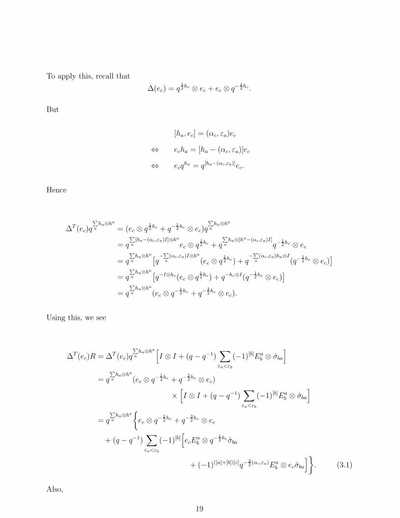
To apply this, recall that

∆(ec) = q12hc ⊗ ec + ec ⊗ q−

12hc .

But

[ha, ec] = (αc, εa)ec

⇔ echa = [ha − (αc, εa)]ec

⇔ ecqha = q[ha−(αc,εa)]ec.

Hence

∆T (ec)q

∑

a

ha⊗ha

= (ec ⊗ q12hc + q−

12hc ⊗ ec)q

∑

a

ha⊗ha

= q

∑

a

[ha−(αc,εa)I]⊗ha

ec ⊗ q12hc + q

∑

a

ha⊗[ha−(αc,εa)I]q−

12hc ⊗ ec

= q

∑

a

ha⊗ha[

q−

∑

a

(αc,εa)I⊗ha

(ec ⊗ q12hc) + q

−∑

a

(αc,εa)ha⊗I(q−

12hc ⊗ ec)

]

= q

∑

a

ha⊗ha[

q−I⊗hc(ec ⊗ q12hc) + q−hc⊗I(q−

12hc ⊗ ec)

]

= q

∑

a

ha⊗ha

(ec ⊗ q−12hc + q−

32hc ⊗ ec).

Using this, we see

∆T (ec)R = ∆T (ec)q

∑

a

ha⊗ha[

I ⊗ I + (q − q−1)∑

εa<εb


]

= q

∑

a

ha⊗ha

(ec ⊗ q−12hc + q−

32hc ⊗ ec)

×[

I ⊗ I + (q − q−1)∑

εa<εb


]

= q

∑

a

ha⊗ha{

ec ⊗ q−12hc + q−

32hc ⊗ ec

+ (q − q−1)∑

εa<εb

(−1)[b][

ecEab ⊗ q−

12hcσba

+ (−1)([a]+[b])[c]q−32(αc,εa)Ea

b ⊗ ecσba

]

}

. (3.1)

Also,

19

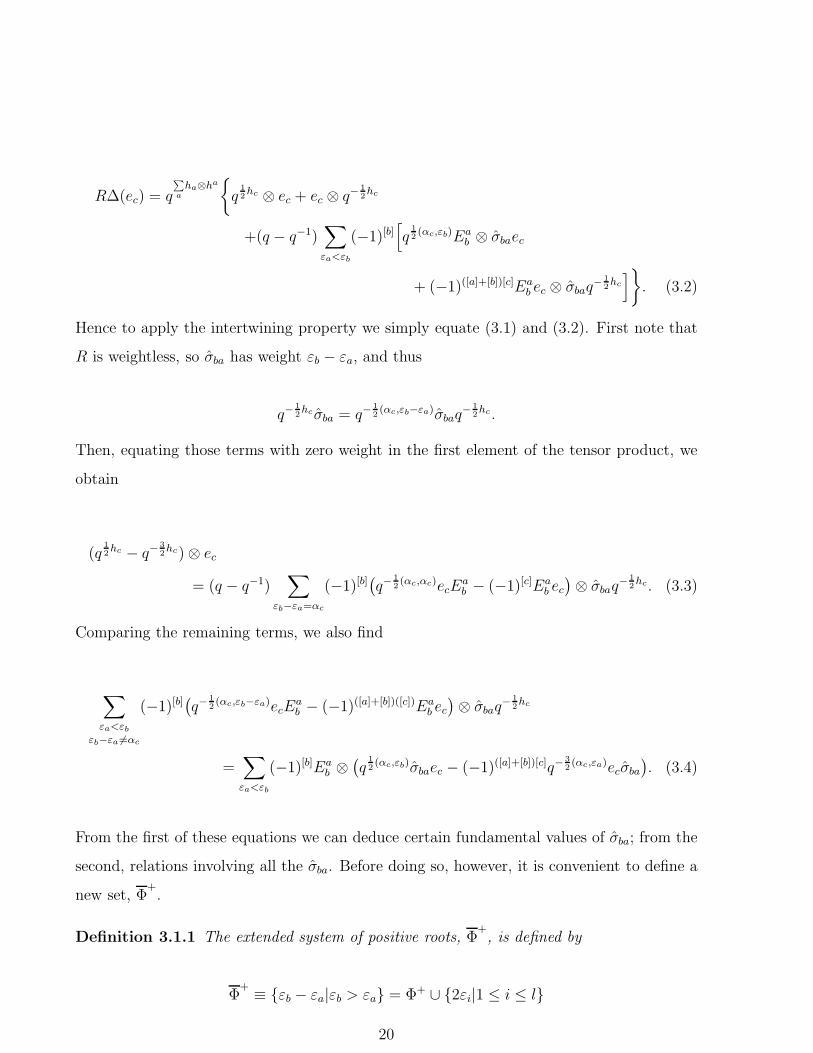
R∆(ec) = q

∑

a

ha⊗ha{

q12hc ⊗ ec + ec ⊗ q−

12hc

+(q − q−1)∑

εa<εb

(−1)[b][

q12(αc,εb)Ea

b ⊗ σbaec

+ (−1)([a]+[b])[c]Eab ec ⊗ σbaq

− 12hc

]

}

. (3.2)

Hence to apply the intertwining property we simply equate (3.1) and (3.2). First note that

R is weightless, so σba has weight εb − εa, and thus

q−12hcσba = q−

12(αc,εb−εa)σbaq

− 12hc .

Then, equating those terms with zero weight in the first element of the tensor product, we

obtain

(q12hc − q−

32hc) ⊗ ec

= (q − q−1)∑

εb−εa=αc

(−1)[b](

q−12(αc,αc)ecE

ab − (−1)[c]Ea

b ec

)

⊗ σbaq− 1

2hc. (3.3)

Comparing the remaining terms, we also find

∑

εa<εb

εb−εa 6=αc

(−1)[b](

q−12(αc,εb−εa)ecE

ab − (−1)([a]+[b])([c])Ea

b ec

)

⊗ σbaq− 1

2hc

=∑

εa<εb

(−1)[b]Eab ⊗

(

q12(αc,εb)σbaec − (−1)([a]+[b])[c]q−

32(αc,εa)ecσba

)

. (3.4)

From the first of these equations we can deduce certain fundamental values of σba; from the

second, relations involving all the σba. Before doing so, however, it is convenient to define a

new set, Φ+.

Definition 3.1.1 The extended system of positive roots, Φ+, is defined by

Φ+≡ {εb − εa|εb > εa} = Φ+ ∪ {2εi|1 ≤ i ≤ l}

20

where Φ+ is the usual system of positive roots.

Now consider equation (3.4). In the case when εb − εa + αc /∈ Φ+, by collecting the terms of

weight εb − εa + αc in the second half of the tensor product we find:

q12(αc,εb)σbaec − (−1)([a]+[b])[c]q−

32(αc,εa)ecσba = 0. (3.5)

Similarly, when εb > εa and εb − εa + αc = εb′ − εa′ ∈ Φ+

we find:

∑

εa′<εb′

εb−εa+αc=εb′−εa′

(−1)[b′](

q−12(αc,εb′−εa′)ecE

a′

b′ − (−1)([a′]+[b′])[c]Ea′

b′ ec

)

⊗ σb′a′q−12hc

= (−1)[b]Eab ⊗

(

q12(αc,εb)σbaec − (−1)([a]+[b])[c])q−

32(αc,εa)ecσba

)

.

However ecEa′

b′ and Eab are linearly independent unless b = b′, as are Ea′

b′ ec and Eab for a 6= a′,

and thus this equation reduces to

∑

εa′<εb

εa′=εa−αc

(−1)[b]q−12(αc,εb−εa′)ecE

a′

b ⊗σba′q−12hc

−∑

εb′>εa

εb′=εb+αc

(−1)[b′]+([a]+[b′])[c]Eab′ec ⊗ σb′aq

− 12hc

= (−1)[b]Eab⊗

(

q12(αc,εb)σbaec − (−1)([a]+[b])[c]q−

32(αc,εa)ecσba

)

.

This can also be written as

q−12(αc,εb−εa+αc)ecE

a′

b ⊗ σba′q−12hc

∣

∣

∣

εa′=εa−αc

− (−1)([a]+[b])[c]Eab′ec ⊗ σb′aq

− 12hc

∣

∣

∣

εb′=εb+αc

= Eab ⊗

(

q12(αc,εb)σbaec − (−1)([a]+[b])[c]q−

32(αc,εa)ecσba

)

, εb > εa.

This equation then implies

21

q−12(αc,εb−εa+αc)〈a|ec|a

′〉σba′q−12hc − (−1)([a]+[b])[c]〈b′|ec|b〉σb′aq

− 12hc

= q12(αc,εb)σbaec − (−1)([a]+[b])[c]q−

32(αc,εa)ecσba, εb > εa.

A more useful form of these relations is:

q−12(αc,αc−εa)〈a|ec|a

′〉σba′ − (−1)([a]+[b])[c]q12(αc,εb)〈b′|ec|b〉σb′a

= q(αc,εb)σbaecq12hc − (−1)([a]+[b])[c]q−

32(αc,εa)+ 1

2(αc,εb)ecσbaq

12hc

= q(αc,εb)σbaecq12hc − (−1)([a]+[b])[c]q−(αc,εa)ecq

12hcσba (3.6)

for εb > εa. All the necessary information is contained within these relations and equation

(3.3). To construct the Lax operator R = (π ⊗ 1)R first we use equation (3.3) to find the

solutions for σba associated with the simple roots αc. Then we apply the recursion relations

arising from (3.6) to find the remaining values of σba.

3.2 Fundamental Values

In this section we solve equation (3.3), rewritten below, to find the fundamental values of

σba, namely those for which εb − εa is a simple root.

(q12hc − q−

32hc) ⊗ ec

= (q − q−1)∑

εb−εa=αc

(−1)[b](

q−12(αc,αc)ecE

ab − (−1)[c]Ea

b ec

)

⊗ σbaq− 1

2hc. (3.3)

To solve this we must consider the various simple roots individually.

Solution for αi = εi − εi+1, 1 ≤ i < l

In the vector representation ei = Eii+1 −Ei+1

iand hi = Ei

i −Ei+1i+1 + Ei+1

i+1− Ei

i.

Hence the left-hand side of (3.3) becomes:

22

LHS = (q12hi − q−

32hi) ⊗ ei

={

(q12 − q−

32 )(Ei

i + Ei+1i+1

) + (q−12 − q

32 )(Ei+1

i+1 + Eii)}

⊗ ei

= (q − q−1){

q−12 (Ei

i + Ei+1i+1

) − q12 (Ei+1

i+1 + Eii)}

⊗ ei,

whereas the right-hand side is:

RHS = (q − q−1)∑

εb−εa=αi

(

q−1eiEab − Ea

b ei

)

⊗ σbaq− 1

2hi

= (q − q−1){

(q−1Eii − Ei+1

i+1) ⊗ σi i+1q− 1

2hi − (q−1Ei+1

i+1− Ei

i) ⊗ σi+1 iq

− 12hi

}

.

Equating these gives

σi i+1 = −σi+1 i = q12 eiq

12hi , 1 ≤ i < l.

Solution for αl = εl−1 + εl, m = 2l

Here el = El−1

l− El

l−1and hl = El

l − Ell+ El−1

l−1 − El−1

l−1. Substituting these into equation

(3.3) gives:

LHS ={

(q12 − q−

32 )(El

l + El−1l−1) + (q−

12 − q

32 )(El

l+ El−1

l−1)}

⊗ el

= (q − q−1){

q−12 (El

l + El−1l−1) − q

12 (El

l+ El−1

l−1)}

⊗ el

and

RHS = (q − q−1){

(q−1El−1l−1 − El

l) ⊗ σl−1 lq

− 12hl − (q−1El

l − El−1

l−1) ⊗ σl l−1q

− 12hl

}

.

Thus

σl−1 l = −σl l−1 = q12elq

12hl, m = 2l.

Solution for αl = εl, m = 2l + 1

23

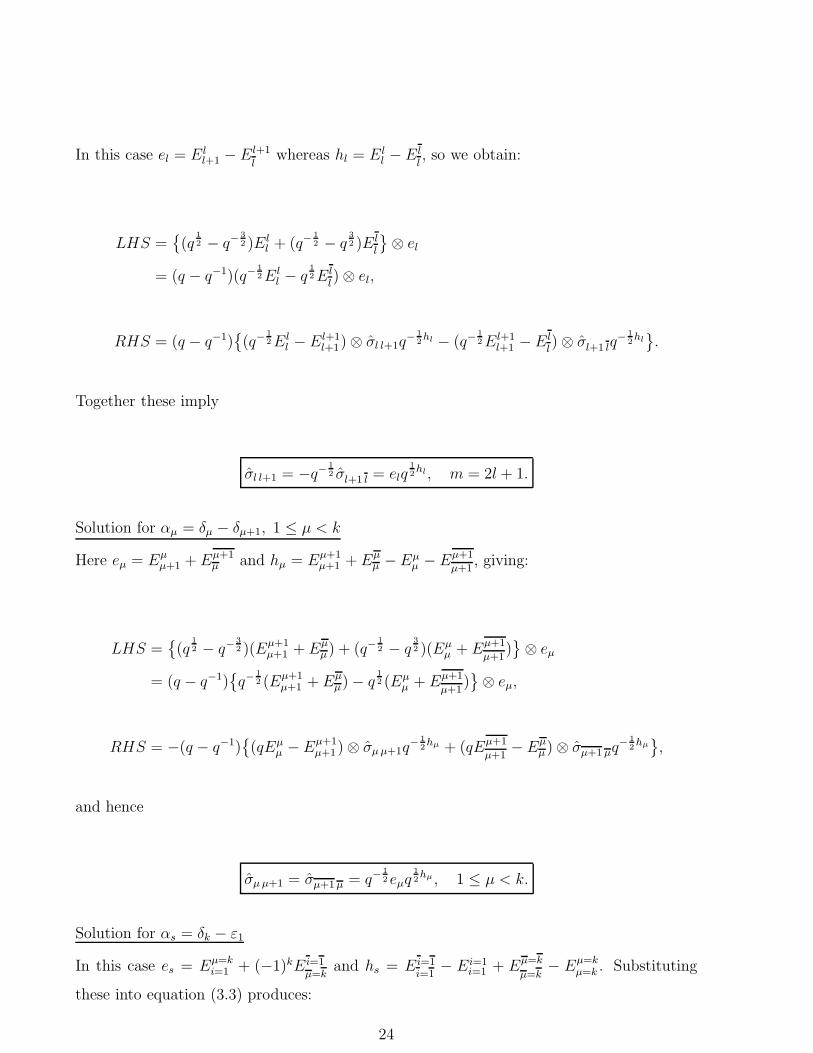
In this case el = Ell+1 − El+1

lwhereas hl = El

l − Ell, so we obtain:

LHS ={

(q12 − q−

32 )El

l + (q−12 − q

32 )El

l

}

⊗ el

= (q − q−1)(q−12El

l − q12El

l) ⊗ el,

RHS = (q − q−1){

(q−12El

l − El+1l+1) ⊗ σl l+1q

− 12hl − (q−

12El+1

l+1 − Ell) ⊗ σl+1 lq

− 12hl

}

.

Together these imply

σl l+1 = −q−12 σl+1 l = elq

12hl, m = 2l + 1.

Solution for αµ = δµ − δµ+1, 1 ≤ µ < k

Here eµ = Eµµ+1 + Eµ+1

µ and hµ = Eµ+1µ+1 + Eµ

µ −Eµµ − Eµ+1

µ+1, giving:

LHS ={

(q12 − q−

32 )(Eµ+1

µ+1 + Eµµ) + (q−

12 − q

32 )(Eµ

µ + Eµ+1

µ+1)}

⊗ eµ

= (q − q−1){

q−12 (Eµ+1

µ+1 + Eµµ) − q

12 (Eµ

µ + Eµ+1

µ+1)}

⊗ eµ,

RHS = −(q − q−1){

(qEµµ − Eµ+1

µ+1) ⊗ σµ µ+1q− 1

2hµ + (qEµ+1

µ+1− Eµ

µ) ⊗ σµ+1 µq− 1

2hµ

}

,

and hence

σµ µ+1 = σµ+1 µ = q−12eµq

12hµ , 1 ≤ µ < k.

Solution for αs = δk − ε1

In this case es = Eµ=ki=1 + (−1)kEi=1

µ=kand hs = Ei=1

i=1− Ei=1

i=1 + Eµ=k

µ=k− Eµ=k

µ=k . Substituting

these into equation (3.3) produces:

24

LHS ={

(q12 − q−

32 )(Ei=1

i=1+ Eµ=k

µ=k) + (q−

12 − q

32 )(Ei=1

i=1 + Eµ=kµ=k )

}

⊗ es

= (q − q−1){

q−12 (Ei=1

i=1 + Eµ=k

µ=k) − q

12 (Ei=1

i=1 + Eµ=kµ=k )

}

⊗ es,

RHS = (q − q−1){

−(Eµ=kµ=k + Ei=1

i=1) ⊗ σµ=k i=1q− 1

2hs

+ (−1)k(Ei=1i=1 + Eµ=k

µ=k) ⊗ σi=1 µ=kq

− 12hs

}

,

and thus

σµ=k i=1 = (−1)kq σi=1 µ=k = q12 esq

12hs.

These values for σba form the basis for finding R, as from these all the others can be explicitly

determined in any given representation.

3.3 Constructing the Non-Simple Values

Now we develop the recurrence relations required to calculate the remaining values of σba.

Recall that for εb > εa,




12hcσba. (3.7)

To extract the recurrence relations to be applied to the fundamental values of σba, we must

again consider the simple roots individually. We begin with the case αi = εi − εi+1, so

ei = σii+1 ≡ Ei

i+1 − Ei+1i

. Now

〈a|ei = δai〈i+ 1| − δa i+1〈i|, ei|b〉 = δb i+1|i〉 − δbi|i+ 1〉.

We then apply that to equation (3.7) to obtain:

25

q−12(αi,αi)

{

δaiq12(αi,εi)σb i+1 − δa i+1q

− 12(αi,εi+1)σb i

}

−{

δb i+1q12(αi,εi+1)σia − δb iq

− 12(αi,εi)σi+1 a

}

=q(αi,εb)σbaeiq12hi − q−(αi,εa)eiq

12hiσba, εb > εa.

This simplifies to

q−12

{

δaiσb i+1 − δa i+1σb i − δb i+1σia + δb iσi+1 a

}

= q(αi,εb)σbaeiq12hi − q−(αi,εa)eiq

12hiσba, εb > εa,

which, recalling that σi i+1 = −σi+1 i = q12 eiq

12hi, 1 ≤ i < l, reduces to

δaiσb i+1 − δa i+1σb i − δb i+1σia + δb iσi+1 a = q(αi,εb)σbaσi i+1 − q−(αi,εa)σi i+1σba

= q−(αi,εa)σi+1 iσba − q(αi,εb)σbaσi+1 i.

From this we can deduce the following relations for 1 ≤ i < l:

σb i+1 = σb iσi i+1 − q−1σi i+1σb i, εb > εi,

σi+1 a = σi+1 iσi a − q−1σi aσi+1 i, εa < −εi,

σb i = q(αi,εb)σb i+1σi+1 i − q−1σi+1 iσb i+1, εb > −εi+1, b 6= i+ 1,

σi a = q−(αi,εa)σi i+1σi+1 a − q−1σi+1 aσi i+1, εa < εi+1, a 6= i+ 1,

σi i+1 + σi+1 i = q−1[

σi i+1, σi+1 i+1

]

, (3.8)

q(αi,εb)σbaσi i+1 − q−(αi,εa)σi i+1σba = 0, εb > εa, a 6= i, i+ 1 and b 6= i+ 1, i.

We then follow the same procedure to find the relations associated with the other simple

roots. A detailed derivation of these relations is included in Appendix A, with a complete

list of the relations derived in this manner given in Tables A.1, A.2 and A.3 on pages 118

and 119.

26

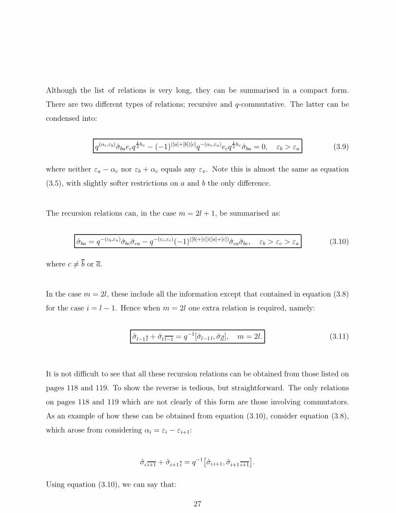
Although the list of relations is very long, they can be summarised in a compact form.

There are two different types of relations; recursive and q-commutative. The latter can be

condensed into:

q(αc,εb)σbaecq12hc − (−1)([a]+[b])[c]q−(αc,εa)ecq

12hcσba = 0, εb > εa (3.9)

where neither εa − αc nor εb + αc equals any εx. Note this is almost the same as equation

(3.5), with slightly softer restrictions on a and b the only difference.

The recursion relations can, in the case m = 2l + 1, be summarised as:

σba = q−(εb,εa)σbcσca − q−(εc,εc)(−1)([b]+[c])([a]+[c])σcaσbc, εb > εc > εa (3.10)

where c 6= b or a.

In the case m = 2l, these include all the information except that contained in equation (3.8)

for the case i = l − 1. Hence when m = 2l one extra relation is required, namely:

σl−1 l + σl l−1 = q−1[σl−1 l, σll], m = 2l. (3.11)

It is not difficult to see that all these recursion relations can be obtained from those listed on

pages 118 and 119. To show the reverse is tedious, but straightforward. The only relations

on pages 118 and 119 which are not clearly of this form are those involving commutators.

As an example of how these can be obtained from equation (3.10), consider equation (3.8),

which arose from considering αi = εi − εi+1:

σi i+1 + σi+1 i = q−1[

σi i+1, σi+1 i+1

]

.

Using equation (3.10), we can say that:

27

σi i+1 = σi i+2σi+2 i+1 − q−1σi+2 i+1σi i+2, i < l − 1,

σi+1 i = σi+1 i+2σi+2 i − q−1σi+2 iσi+1 i+2, i < l − 1,

σi+2 i = σi+2 i+1σi+1 i − q−1σi+1 iσi+2 i+1, i < l − 1,

σi i+2 = σi i+1σi+1 i+2 − q−1σi+1 i+2σi i+1, i < l − 1,

σi+1 i+1 = qσi+1 i+2σi+2 i+1 − q−1σi+2 i+1σi+1 i+2, i < l − 1.

Combining these, we find that for i < l − 1

σi i+1 + σi+1 i = σi i+2σi+2 i+1 + σi+1 i+2σi+2 i − q−1σi+2 i+1σi i+2 − q−1σi+2 iσi+1 i+2

= σi i+2σi+2 i+1 + σi+1 i+2

(

σi+2 i+1σi+1 i − q−1σi+1 iσi+2 i+1

)

− q−1σi+2 i+1

(

σi i+1σi+1 i+2 − q−1σi+1 i+2σi i+1

)

− q−1σi+2 iσi+1 i+2

=(

σi i+2 − q−1σi+1 i+2σi+1 i

)

σi+2 i+1 − q−1(

σi+2 i + σi+2 i+1σi i+1

)

σi+1 i+2

+ σi+1 i+2σi+2 i+1σi+1 i + q−2σi+2 i+1σi+1 i+2σi i+1

=(

σi i+2 + q−1σi+1 i+2σi i+1

)

σi+2 i+1 − q−1(

σi+2 i − σi+2 i+1σi+1 i

)

σi+1 i+2

−(

σi+1 i+2σi+2 i+1 − q−2σi+2 i+1σi+1 i+2

)

σi i+1

= σi i+1σi+1 i+2σi+2 i+1 + q−2σi+1 iσi+2 i+1σi+1 i+2 − q−1σi+1 i+1σi i+1

= σi i+1

(

σi+1 i+2σi+2 i+1 − q−2σi+2 i+1σi+1 i+2

)

− q−1σi+1 i+1σi i+1

= q−1σi i+1σi+1 i+1 − q−1σi+1 i+1σi i+1

= q−1[σi i+1, σi+1 i+1]

as required. Note that this working also holds true for i = l − 1 in the case m = 2l + 1,

as then the conditions on equation (3.10) are all met. In the case m = 2l, however, there

is no way to meet the conditions to find an expansion of σl−1 l or σl l−1, which is why the

extra relation (3.11) must be included. The technique used above can be applied almost

identically to find the commutation relations that arose from the roots αµ and αs. Hence

equations (3.9), (3.10) and (3.11) are equivalent to the complete set of q-commutation and

recursion relations derived in Appendix A.

28

In the case m = 2l, we can find an alternative extra relation to equation (3.11). For such

m, consider the relations involving σl l.

Firstly, we have

q(αi,εb)σbaσi i+1 − q−(αi,εa)σi i+1σba = 0, εa < εb, a 6= i, i+ 1 and b 6= i, i+ 1

⇒ [σi i+1, σl l] = 0, i < l − 1

and

q(αl,εb)σbaσl−1 l − q−(αl,εa)σl−1 lσba = 0, εa < εb, a 6= l − 1, l and b 6= l − 1, l

⇒ [σl−1 l, σl l] = 0.

Moreover, we know

[σl−1 l, σl l] = q(σl−1 l + σl l−1)

⇔ [σl−1 l, σl l] = 0

from the simple generators in Section 3.2. Similarly, σl l can be shown to commute with

the remaining simple generators. Together these imply σl l is an invariant of the system. It

cannot, therefore, have weight 2εl, as it would if it were non-zero, so

σl l = 0, m = 2l.

This equation is a convenient alternative to (3.11) in the unified form of the relations.

Hence we have found the following result:

29

Lemma 3.3.1 There is a unique matrix in (End V ) ⊗ Uq[osp(m|n)]+ of the form

R = q

∑

a

ha⊗ha[

I ⊗ I + (q − q−1)∑

εa<εb


]

,

satisfying R∆(ec) = ∆T (ec)R. The fundamental values of σba for that matrix are given by:

σi i+1 = −σi+1 i = q12eiq

12hi, 1 ≤ i < l,

σl−1 l = −σl l−1 = q12elq

12hl, m = 2l,

σl l = 0, m = 2l,

σl l+1 = −q−12 σl+1 l = elq

12hl, m = 2l + 1,


12hµ , 1 ≤ µ < k,

σµ=k i=1 = (−1)kq σi=1 µ=k = q12 esq

12hs; (3.12)

30

and the remaining values can be calculated using

(i) the q-commutation relations


12hcσba = 0, εb > εa, (3.13)

where neither εa − αc nor εb + αc equals any εx; and

(ii) the induction relations

σba = q−(εb,εa)σbcσca − q−(εc,εc)(−1)([b]+[c])([a]+[c])σcaσbc, εb > εc > εa, (3.14)

where c 6= b or a.

This matrix can also be written in a slightly different form. As we are working in the (π⊗ id)

representation, we have

q

∑

a

ha⊗ha

= (∑

a

Eaa ⊗ I)q

∑

b

hb⊗hb

= (∑

a

Eaa ⊗ I)q

∑

b

(εa,εb)I⊗hb

=∑

a

Eaa ⊗ qhεa .

Hence an alternative way of expressing R is

R =∑

a

Eaa ⊗ qhεa + (q − q−1)

∑

εa<εb

(−1)[b]Eab ⊗ qhεa σba,

with the σba as given before.

31

Chapter 4

A Closer Look at the Lax operator

We have found a set of fundamental values and relations which uniquely define the unknowns

σba. Theoretically the resultant matrix R must be a Lax operator, as we know there is one

of the given form. It seems advisable, however, to check this by verifying that R satisfies

the remaining R-matrix properties. These are

(id ⊗ ∆)R = R13R12 (4.1)

and the intertwining property for the remaining generators,

R∆(a) = ∆T (a)R, ∀a ∈ Uq[osp(m|n)].

In this chapter we confirm that R satisfies both these properties. We also calculate the

opposite Lax operator RT , and briefly examine whether the defining relations for the σba

incorporate the q-Serre relations for Uq[osp(m|n)].

4.1 Calculating the Coproduct

We begin by considering the first of these defining properties, equation (4.1). In order to

evaluate (id ⊗ ∆)R, however, we need to know ∆(σba). Now at the end of the previous

chapter we showed that

33

R =∑

a


∑

εb>εa

(−1)[b]Eab ⊗ qhεa σba.

Using this form for R, we find

R13R12 =(

∑

a

Eaa ⊗ I ⊗ qhεa + (q − q−1)

∑

εb>εa

(−1)[b]Eab ⊗ I ⊗ qhεa σba

)

(

∑

c

Ecc ⊗ qhεc ⊗ I + (q − q−1)

∑

εd>εc

(−1)[d]Ecd ⊗ qhεc σdc ⊗ I

)

=∑

a

∑

c

EaaE

cc ⊗ qhεc ⊗ qhεa

+ (q − q−1)∑

a

∑

εd>εc

(−1)[d]EaaE

cd ⊗ qhεc σdc ⊗ qhεa

+ (q − q−1)∑

c

∑

εb>εa

(−1)[b]EabE

cc ⊗ qhεc ⊗ qhεa σba

+ (q − q−1)2∑

εb>εa

∑

εd>εc

(−1)[b]+[d]EabE

cd ⊗ qhεc σdc ⊗ qhεa σba

=∑

a

Eaa ⊗ qhεa ⊗ qhεa + (q − q−1)

∑

εd>εc

(−1)[d]Ecd ⊗ qhεc σdc ⊗ qhεc

+ (q − q−1)∑

εb>εa

(−1)[b]Eab ⊗ qhεb ⊗ qhεa σba

+ (q − q−1)2∑

εd>εc>εa

(−1)[c]+[d]Ead ⊗ qhεc σdc ⊗ qhεa σca

=∑

a

Eaa ⊗ qhεa ⊗ qhεa

+ (q − q−1)∑

εb>εa

(−1)[b]Eab ⊗

(

qhεa σba ⊗ qhεa + qhεb ⊗ qhεa σba

)

+ (q − q−1)2∑

εb>εc>εa

(−1)[b]+[c]Eab ⊗ qhεc σbc ⊗ qhεa σca.

Also, the coproduct properties (2.6) imply

(id ⊗ ∆)R =∑

a

Eaa ⊗ qhεa ⊗ qhεa + (q − q−1)

∑

εb>εa

(−1)[b]Eab ⊗ (qhεa ⊗ qhεa)∆(σba).

Hence R will satisfy equation (4.1) if and only if ∆(σba) is given by:

34

∆(σba) = σba ⊗ I + qhεb−hεa ⊗ σba + (q − q−1)

∑

εb>εc>εa

(−1)[c]qhεc−hεa σbc ⊗ σca.

Now we use the fundamental values of σba (3.12) and the inductive relations (3.14) to calcu-

late ∆(σba), and show that it is indeed of this form. First set

hba ≡ hεb− hεa

,

so we need to show

∆(σba) = σba ⊗ I + qhba ⊗ σba + (q − q−1)∑

εb>εc>εa

(−1)[c]qhcaσbc ⊗ σca.

Consider the non-zero fundamental values of σba, given in equation (3.12). For these values

αb = εb − εa is a simple root. Note that in each case σba = Aebq12hba or Aeaq

12hba for some

constant A. Then

∆(σba) = A∆(ec)∆(q12hba), c = b or a

= A(q12hba ⊗ ec + ec ⊗ q−

12hba)(q

12hba ⊗ q

12hba)

= qhba ⊗ Aecq12hb + Aecq

12hb ⊗ I

= qhba ⊗ σba + σba ⊗ I.

In the case of a simple root there is usually no c satisfying εb > εc > εa, so this is the expected

result. The only exceptions to that generalisation are σl l−1 and σl−1 l where m = 2l. In both

those cases, however, the sum in our expression for ∆(σba) still disappears as it becomes a

single term containing σl l, which we know equals 0. Hence our formula for the expected

coproduct is correct for the non-zero fundamental values of σba.

Also, when m = 2l

σll ⊗ I + qhll ⊗ σll + (q − q−1)

∑

εl>εc>−εl

(−1)[c]qhclσlc ⊗ σcl = 0 + 0 + 0 = ∆(σll = 0)

35

as required. Thus we have verified the formula for the coproduct for all the fundamental

values of σba given in equation (3.12).

To find the coproduct for the remaining values of σba we use the inductive relations (3.14):

σba = q−(εb,εa)σbcσca − q−(εc,εc)(−1)([b]+[c])([a]+[c])σcaσbc, εb > εc > εa,

where c 6= b or a. We assume our formula for the coproduct holds for σbc and σca, where

εb > εc > εa, and then show it is also true for σba.

We can always choose c satisfying the conditions such that either εb − εc or εc − εa is a

simple root. First consider εb − εc is a simple root, denoted by either αb or αc depending on

circumstance, so σbc = Aebq12hb or Aecq

12hc for some constant A.

The coproduct is an algebra homomorphism, so for εb > εc > εa, c 6= a or b, we have

∆(σba) = q−(εb,εa)∆(σbc)∆(σca) − q−(εc,εc)(−1)([b]+[c])([a]+[c])∆(σca)∆(σbc).

Substituting in our expression for the coproduct gives:

∆(σba) =q−(εb,εa)(σbc ⊗ I + qhbc ⊗ σbc)

(

σca ⊗ I + qhca ⊗ σca + (q − q−1)∑

εc>εd>εa

(−1)[d]qhdaσcd ⊗ σda

)

− q−(εc,εc)(−1)([b]+[c])([a]+[c])

(

σca ⊗ I + qhca ⊗ σca + (q − q−1)∑

εc>εd>εa

(−1)[d]qhdaσcd ⊗ σda

)

(σbc ⊗ I + qhbc ⊗ σbc).

Expanding, we obtain

36

∆(σba) = (q−(εb,εa)σbcσca − q−(εc,εc)(−1)([b]+[c])([a]+[c])σcaσbc) ⊗ I

+ qhba ⊗ (q−(εb,εa)σbcσca − q−(εc,εc)(−1)([b]+[c])([a]+[c])σcaσbc)

+ (q−(εb,εa)q−(εc−εa,εb−εc) − q−(εc,εc)[(−1)([b]+[c])([a]+[c])]2)qhcaσbc ⊗ σca

+(

q−(εb,εa)(−1)([b]+[c])([a]+[c])

− q−(εc,εc)(−1)([b]+[c])([a]+[c])q−(εb−εc,εc−εa))

qhbcσca ⊗ σbc

+ (q − q−1)∑

εc>εd>εa

(−1)[d]qhdaq−(εb,εa)q−(εd−εa,εb−εc)σbcσcd ⊗ σda

− (q − q−1)∑

εc>εd>εa

(−1)[d]qhdaq−(εc,εc)(−1)([b]+[c])([c]+[d])σcdσbc ⊗ σda

+ (q − q−1)∑

εc>εd>εa

(−1)[d]qhbc+hdaq−(εb,εa)(−1)([b]+[c])([c]+[d])σcd ⊗ σbcσda

− (q − q−1)∑

εc>εd>εa

(−1)[d]qhbc+hdaq−(εc,εc)(−1)([b]+[c])([a]+[c])

× q−(εb−εc,εc−εd)σcd ⊗ σdaσbc.

Since εb > εc > εa and c 6= a or b, we know that (εa, εc) = (εb, εc) = 0. Using this, we

simplify the above expression to:

∆(σba) =σba ⊗ I + qhba ⊗ σba + (q(εc,εc) − q−(εc,εc))qhcaσbc ⊗ σca

+ (q−(εb,εa) − q(εb,εa))(−1)([b]+[c])([a]+[c])qhbcσca ⊗ σbc

+ (q − q−1)∑

εc>εd>εa

(−1)[d]qhda(

q−(εd,αb)σbcσcd

− q−(εc,εc)(−1)([b]+[c])([c]+[d])σcdσbc

)

⊗ σda

+ (q − q−1)∑

εc>εd>εa

(−1)[d]qhda+hbc(−1)([b]+[c])([a]+[c])σcd

⊗(

q−(εb−εc,εa)(−1)([b]+[c])([a]+[d])σbcσda − q(εd,αb)σdaσbc

)

. (4.2)

But when d 6= b the q-commutation relations (3.13) can be used to show

37

q−(αb,εa)(−1)([b]+[c])([a]+[d])σbcσda − q(εd,αb)σdaσbc

= − A(q(εd,αb)σdaebq12hb − (−1)([a]+[d])[αb]q−(αb,εa)ebq

12hbσda)

(

or − A(q(εd,αc)σdaecq12hc − (−1)([a]+[d])[αc]q−(αc,εa)ebq

12hcσda)

)

= 0.

And in the case c 6= d, we have

q−(εd,αb)σbcσcd − q−(εc,εc)(−1)([b]+[c])([c]+[d])σcdσbc = σbd

from the inductive relations (3.14). Moreover, when c = d (so εc > 0) we note from the

relations in Table A.1 that

q−(εd,αb)σbcσcd − q−(εc,εc)(−1)([b]+[c])([c]+[d])σcdσbc

= q−(εc,εc)[σbc, σc c]

= σbc + (−1)[b][(−1)kq]δci=1σcb

= σbd + (−1)[b][(−1)kq]δci=1 σcb,

so for all d satisfying εc > εd > εa we have

q−(εd,αb)σbcσcd − q−(εc,εc)(−1)([b]+[c])([c]+[d])σcdσbc = σbd + δcd(−1)[b][(−1)kq]δ

ci=1 σcb.

We also introduce a new function θxy, defined by

θxy =

1, εx > εy,

0, εx ≤ εy.

Combining all this information, we simplify equation (4.2) to:

38

∆(σba) =σba ⊗ I + qhba ⊗ σba + (1 − δci=l+1)(q − q−1)(−1)[c]qhca σbc ⊗ σca

+ δab(q − q−1)(−1)[c]qhbcσca ⊗ σbc

+ (q − q−1)∑

εc>εd>εa

(−1)[d]qhdaσbd ⊗ σda

+ (q − q−1)(−1)[c]+[b]θccθcaqhca [(−1)kq]δ

ci=1σcb ⊗ σca

+ (q − q−1)(−1)[c]θcbθbaqhca σcb ⊗ (σbcσba − (−1)([b]+[c])([a]+[b])q−(εb,εb)σbaσbc). (4.3)

While this currently does not look much like the expected formula for ∆(σba), it can be

further simplified. First note that since εb − εc = εc − εb is a simple root,

θccθca = θccθcbθba + δabθccθca + θccθcaθab

= θccθba + δabθcc

and

θcbθba = θccθcbθba + δccθcbθba + θccθcbθba

= θccθba + δci=l+1θla + δb

i=l−1δcj=lθl−1 a.

Also, looking back at the formulae for σbc associated with the simple roots, we see that if

δci=l+1 = 1 we have σbc = −q−

12σcb; if δb

i=l−1δcj=l

= 1 then σbc = −σcb; and if θcc = 1 then

σbc = −(−1)[b][(−1)kq]δci=1σcb. Moreover, if θcbθba = 1 then b 6= c, a so we can simplify the

final term in (4.3) using

σca = σc bσba − (−1)([b]+[c])([a]+[b])q−(εb,εb)σbaσc b.

Applying all this gives:

39

∆(σba) =σba ⊗ I + qhba ⊗ σba + (q − q−1)∑

εc≥εd>εa


− δci=l+1(q − q−1)qhcaσbc ⊗ σca + δa

b(q − q−1)(−1)[c]qhbcσca ⊗ σbc

+ (q − q−1)(−1)[b]+[c](θccθba + δabθcc)q

hca [(−1)kq]δci=1 σcb ⊗ σca

− (q − q−1)(−1)[b]+[c][(−1)kq]δci=1θccθbaq

hca σcb ⊗ σca

− δci=l+1(q − q−1)q−

12θlaq

hcaσc b ⊗ σca

− δbi=l−1δ

cj=l

(q − q−1)θl−1aqhla σl l−1 ⊗ σla

=σba ⊗ I + qhba ⊗ σba + (q − q−1)∑

εc≥εd>εa


− δci=l+1δ

ab(q − q−1)(−1)[c]qhbcσca ⊗ σbc + δa

b(q − q−1)(−1)[c]qhbcσca ⊗ σbc

− δab(q − q−1)(−1)[c]θccq

hbcσca ⊗ σbc

+ δbi=l−1δ

cj=l

(q − q−1)θl−1aqhlaσl−1 l ⊗ σla.

Now note that

δab(1 − δc

i=l+1 − θcc) = δabδbi=l−1δ

cj=l

and that σll = 0. Then our formula for ∆(σba) becomes:

∆(σba) =σba ⊗ I + qhba ⊗ σba + (q − q−1)∑

εc≥εd>εa


+ δabδbi=l−1δ

cj=l

(q − q−1)(−1)[c]qhbcσca ⊗ σbc

+ δbi=l−1δ

cj=l

(q − q−1)θl−1aqhlaσl−1 l ⊗ σla

+ δbi=lδ

cj=l−1

(q − q−1)θlaqh

la σll ⊗ σla

=σba ⊗ I + qhba ⊗ σba + (q − q−1)∑

εc≥εd>εa


+ δbi=l−1δ

cj=l

(q − q−1)θlaqhlaσl−1 l ⊗ σla

+ δbi=lδ

cj=l−1

(q − q−1)θl−1aqh

la σll ⊗ σla

=σba ⊗ I + qhba ⊗ σba + (q − q−1)∑

εb>εd>εa


40

as required.

To verify our formula for the coproduct it is also necessary to consider the case when σca is

a fundamental value. The calculations, however, are extremely similar to those where σbc is

a fundamental value, so they are not included. Suffice it to say that they give the expected

result. Moreover, as a check, it has also been shown directly that the coproduct is consistent

with the commutation relations (3.13), although again the calculations are rather tedious

and have been omitted.

Thus we have shown the coproduct of the operators σba is given by

∆(σba) = σba ⊗ I + qhba ⊗ σba + (q − q−1)∑

εb>εc>εa

(−1)[c]qhcaσbc ⊗ σca,

and consequently that the matrix R found in the previous chapter satisfies the property

(id ⊗ ∆)R = R13R12.

4.2 The Intertwining Property

To confirm that we have a Lax operator we need to check one last relation, namely the

intertwining property for the other generators.

R∆(a) = ∆T (a)R, ∀a ∈ Uq[osp(m|n)]. (4.4)

Now R is weightless, so it commutes with all the Cartan elements. Moreover, ∆(qha) =

∆T (qha), ∀ha ∈ H , so the Cartan elements will automatically satisfy equation (4.4). Thus

it remains only to verify the intertwining property for the lowering generators, fa. Unfor-

tunately, knowing the raising generators satisfy the intertwining property does not appear

helpful. Instead, we start by assuming the form of the Lax operator and that it satisfies

the intertwining property for the lowering generators, and then proceed as in the previous

chapter. Provided the relations and fundamental values obtained are consistent with those

41

already developed, we will have confirmed that the matrix R constructed in the previous

chapter is a Lax operator. Initially the process mirrors that in Section 3.1, so some of the

detail is omitted.

Now we know

R ≡ q

∑

a

ha⊗ha[

I ⊗ I + (q − q−1)∑

εa<εb


]

and

∆(fc) = q12hc ⊗ fc + fc ⊗ q−

12hc.

Moreover,

∆T (fc)q

∑

a

ha⊗ha

= (q−12hc ⊗ fc + fc ⊗ q

12hc)q

∑

a

ha⊗ha

= q

∑

a

ha⊗ha

(q12hc ⊗ fc + fc ⊗ q

32hc).

Therefore

∆T (fc)R

= q

∑

a

ha⊗ha

(q12hc ⊗ fc + fc ⊗ q

32hc)

[

I ⊗ I + (q − q−1)∑

εa<εb


]

= q

∑

a

ha⊗ha{

q12hc ⊗ fc + fc ⊗ q

32hc

+ (q − q−1)∑

εa<εb

(−1)[b][

(−1)([a]+[b])[c]q12(αc,εa)Ea

b ⊗ fcσba + fcEab ⊗ q

32hcσba

]

}

, (4.5)

while

R∆(fc) = q

∑

aha⊗ha{

q12hc ⊗ fc + fc ⊗ q−

12hc

+(q − q−1)∑

εa<εb

(−1)[b][

q12(αc,εb)Ea

b ⊗ σbafc

+ (−1)([a]+[b])[c]Eab fc ⊗ σbaq

− 12hc

]

}

. (4.6)

42

Equating (4.5) and (4.6), we find

fc ⊗ (q32hc − q−

12hc)

= (q − q−1)∑

εa<εb

(−1)[b][

q12(αc,εb)Ea

b ⊗ σbafc − (−1)([a]+[b])[c]q12(αc,εa)Ea

b ⊗ fcσba

]

+ (q − q−1)∑

εa<εb

(−1)[b][

(−1)([a]+[b])[c]Eab fc ⊗ σbaq

− 12hc − fcE

ab ⊗ q

32hcσba

]

. (4.7)

Taking the terms with zero weight on the right-hand side of the tensor product gives

fc ⊗ (q32hc − q−

12hc)

= (q − q−1)∑

εb−εa=αc

(−1)[b]Eab ⊗

(

q12(αc,εb)σbafc − (−1)[c]q

12(αc,εa)fcσba

)

. (4.8)

This can be used to find the fundamental values of σba, and check that they agree with those

in Section 3.2.

Similarly, taking the terms of Equation (4.7) with non-zero weight on the right-hand side of

the tensor product, we find

∑

εb>εa

εb−εa 6=αc

(−1)[b]Eab ⊗

(

q12(αc,εb)σbafc − (−1)([a]+[b])[c]q

12(αc,εa)fcσba

)

=∑

εb>εa

(−1)[b](

fcEab ⊗ q

32hcσba − (−1)([a]+[b])[c]Ea

b fc ⊗ σbaq− 1

2hc

)

.

When εb − εa − αc /∈ Φ+

(recalling that Φ+

= {εb − εa|εb > εa}), this gives


12(αc,εa)fcσba = 0.

Conversely, when εb − εa − αc = εb′ − εa′ we obtain

43

∑

εb′>εa′

εb−εa−αc=εb′−εa′

(−1)[b′](

fcEa′

b′ ⊗ q32hcσb′a′ − (−1)([a′]+[b′])[c]Ea′

b′ fc ⊗ σb′a′q−12hc

)

= (−1)[b]Eab ⊗

(


12(αc,εa)fcσba

)

, εb > εa.

However Eab and fcE

a′

b′ are linearly independent unless b = b′, as are Eab and Ea′

b′ fc when

a 6= a′. Hence we can simplify this equation to

∑

εb>εa′

εa′=εa+αc

(−1)[b]fcEa′

b ⊗ q32hcσba′ −

∑

εb′>εa

εb′=εb−αc

(−1)[b′](−1)([a]+[b′])[c]Eab′fc ⊗ σb′aq

− 12hc

= (−1)[b]Eab ⊗

(


12(αc,εa)fcσba

)

, εb > εa.

This then reduces to

(−1)[b]q32(εb−εa−αc,αc)fcE

a′

b ⊗ σba′q32hc

∣

∣

∣

εa′=εa+αc

− (−1)[b]+[c](−1)([a]+[b]+[c])[c]Eab′fc ⊗ σb′aq

− 12hc

∣

∣

∣

εb′=εb−αc

= (−1)[b]Eab ⊗

(


12(αc,εa)fcσba

)

for εb > εa, which can, in turn, be simplified to

q32(εb−εa−αc,αc)〈a|fc|a

′〉σba′q32hc − (−1)([a]+[b])[c]〈b′|fc|b〉σb′aq

− 12hc

= q12(αc,εb)σbafc − (−1)([a]+[b])[c]q

12(αc,εa)fcσba, εb > εa. (4.9)

We now test whether equations (4.8) and (4.9) are consistent with the σba found in the

preceding chapter. Firstly, we use the former to check the fundamental values of σba.

fc ⊗ (q32hc − q−

12hc)

= (q − q−1)∑

εb−εa=αc

(−1)[b]Eab ⊗

(

q12(αc,εb)σbafc − (−1)[c]q

12(αc,εa)fcσba

)

.

44

Consider the case of the root αi = εi − εi+1, 1 ≤ i < l, so fi ≡ Ei+1i − Ei

i+1. Then the

equation becomes:

(Ei+1i −Ei

i+1) ⊗ (q32hi − q−

12hi) = (q − q−1)Ei+1

i ⊗ (q12 σi i+1fi − q−

12 fiσi i+1)

+ (q − q−1)Eii+1

⊗ (q12 σi+1 ifi − q−

12 fiσi+1 i).

Hence we can see immediately that σi i+1 = −σi+1 i, and that

qhi − q−hi = (q − q−1)(q12 σi i+1fiq

− 12hi − q−

12fiσi i+1q

− 12hi)

∴

qhi − q−hi

q − q−1= q−

12 σi i+1q

− 12hifi − q−

12 fiσi i+1q

− 12hi

∴ [ei, fi] = [q−12 σi i+1q

− 12hi , fi].

This is certainly consistent with

σi i+1 = −σi+1 i = q12eiq

12hi,

the formula obtained in Section 3.2. Similarly, we can check all the other fundamental values

using the same method, and in each case they are consistent with those previously obtained.

Thus it only remains to check that the relations arising out of the equation

q32(εb−εa−αc,αc)〈a|fc|a

′〉σba′q32hc − (−1)[c]([a]+[b])〈b′|fc|b〉σb′aq

− 12hc

= q12(αc,εb)σbafc − (−1)[c]([a]+[b])q

12(αc,εa)fcσba, εb > εa

are consistent with relations (3.13) and (3.14) from the previous chapter.

Again, consider the root αi = εi − εi+1, 1 ≤ i < l. Here fi = σi+1i ≡ Ei+1

i −Eii+1

. Then

〈a|fi = δai+1〈i| − δa

i〈i+ 1|, fi|b〉 = δb

i |i+ 1〉 − δbi+1

|i〉.

Hence our equation becomes:

45

q32[(εb,αi)−1](δa

i+1σbi − δaiσb i+1)q

32hi − (δb

i σi+1 a − δbi+1σi a)q

− 12hi

= q12(αi,εb)σbafi − q

12(αi,εa)fiσba, εb > εa.

From this we can deduce the following relations:

q−32 σbiq

32hi = σb i+1fi − q−

12fiσb i+1, εb > εi, (4.10)

q−32 q

32(εb,αi)σb i+1q

32hi = q−

12fiσb i − q

12(αi,εb)σb ifi, b 6= i, εb > −εi+1,

σi+1 aq− 1

2hi = q

12(αi,εa)fiσia − q

12 σiafi, a 6= i, εa < εi+1,

σi aq− 1

2hi = q

12 σi+1 afi − fiσi+1 a, εa < −εi,

σi i+1q32hi + σi+1 iq

− 12hi = q−

12fiσi i − q

12 σi ifi,

q12(αi,εb)σbafi − q

12(αi,εa)fiσba = 0, εb > εa; a 6= i+ 1, i; b 6= i, i+ 1. (4.11)

Unlike the relations obtained in the previous chapter, these cannot be used to inductively

construct the σba. Also, there is no simple general form. Neither of these is a problem,

however, since we only need to confirm that these relations are consistent with those in

Chapter 3.

For instance, consider relation (4.10). Previously we found

σb i+1 = σbiσi i+1 − q−1σi i+1σbi.

Using this, we find that

RHS = σb i+1fi − q−12fiσb i+1

= (σbiσi i+1 − q−1σi i+1σbi)fi − q−12 fi(σbiσi i+1 − q−1σi i+1σbi)

= q12 σbieiq

12hifi − q−

12eiq

12hiσbifi − fiσbieiq

12hi + q−1fieiq

12hiσbi.

Note from equation (4.11) that whenever εb > εi,

46

σbifi = q12fiσbi.

Applying this together with the usual commutation relations, we see

RHS = q−12 σbieifiq

12hi − eiq

12hifiσbi − q−

12 σbifieiq

12hi

+ q−1(

eifi −qhi − q−hi

q − q−1

)

q12hiσbi

= q−12 σbieifiq

12hi − q−1eifiq

12hiσbi − q−

12 σbi

(


q − q−1

)

q12hi

+ q−1(


q − q−1

)

q12hiσbi

=1

q − q−1

[

q−12 σbi(q

32hi − q−

12hi) − q−1(q

32hi − q−

12hi)σbi

]

=1

q − q−1

[

q−12 σbi(q

32hi − q−

12hi) − q−1σbi(q

32(αi,εb−εi)q

32hi − q−

12(αi,εb−εi)q−

12hi)

]

=q−

12 − q−

52

q − q−1σbiq

32hi

= q−32 σbiq

32hi

as expected. Hence equation (4.10) is consistent with the defining relations for σba found in

the previous chapter.

Although time-consuming, it can be confirmed that all the other relations generated by

equation (4.9) are similarly consistent, regardless of which root is chosen. Thus we have

verified that the matrix R constructed in the previous chapter satisfies the intertwining

property

R∆(a) = ∆T (a)R

for all elements a ∈ Uq[osp(m|n)].

47

4.3 The Lax Operator

We have now proven, as expected, that the matrix R found in the previous chapter satisfies

both the intertwining property and (id ⊗ ∆)R = R13R12. The other R-matrix property,

containing (∆ ⊗ id)R, is clearly not applicable here. It is not necessary, however, as we

know there is a Lax operator belonging to π(

Uq[osp(m|n)]−)

⊗ Uq[osp(m|n)]+, and we have

shown there is only one such possibility. Thus the work in this chapter confirms the following

theorem:

Theorem 4.3.1 The Lax operator, R = (π⊗id)R for the quantum superalgebra Uq[osp(m|n)],

where R ∈ Uq[osp(m|n)]− ⊗ Uq[osp(m|n)]+ and m > 2, is given by

R = qhx⊗hx[

I ⊗ I + (q − q−1)∑

εa<εb


]

=∑

a


∑

εa<εb


where the operators σba satisfy:

(i) the q-commutation relations


12hcσba = 0, εb > εa

when neither εa − αc nor εb + αc equals any εx; and

(ii) the recursion relations

σba = q−(εb,εa)σbcσca − q−(εc,εc)(−1)([b]+[c])([a]+[c])σcaσbc, εb > εc > εa

when c 6= b or a; and with initial values given by:

48

σi i+1 = −σi+1 i = q12 eiq

12hi, 1 ≤ i < l,

σl−1 l = −σl l−1 = q12 elq

12hl, m = 2l,

σl l+1 = −q−12 σl+1 l = elq

12hl, m = 2l + 1,

σµ µ+1 = σµ+1 µ = q−12 eµq

12hµ, 1 ≤ µ < k,

σµ=k i=1 = (−1)kq σi=1µ=k = q12 esq

12hs,

σl l = 0, m = 2l.

As an aside, the two properties verified directly are sufficient to prove R satisfies the Yang-

Baxter equation. For using only those, we see

R23R13R12 = R23(id ⊗ ∆)R

= [(id ⊗ ∆T )R]R23

= [(id ⊗ T )((id ⊗ ∆)R]R23

= [(id ⊗ T )R13R12]R23

= R12R13R23

as required.

It is very surprising that there is a unique solution to

R∆(ec) = ∆T (ec)R,

even given we restricted ourselves to matrices in π(

Uq[osp(m|n)]−)

⊗ Uq[osp(m|n)]+. While

it is reassuring that the solution is a Lax operator, it means the remaining R-matrix relations

were redundant, which raises the question of why. It suggests there may be some underlying

symmetries in the system; some way in which the other R-matrix properties can be derived

from the one used. If so, however, they are not obvious.

49

4.4 The Opposite Lax Operator

Having found the Lax operator R = (π⊗ id)R, we wish to use that result to find its opposite

RT = (π ⊗ id)RT , where RT is the opposite universal R-matrix of Uq[osp(m|n)]. We begin

by showing that RT is in fact equal to R†, where † represents graded conjugation, defined

below.

A graded conjugation on Uq[osp(m|n)] is defined on the simple generators by:

e†a = fa, f †a = (−1)[a]ea, h†a = ha.

It is consistent with the coproduct and extends naturally to all remaining elements of

Uq[osp(m|n)], satisfying the properties:

(σab )

† = (−1)[a]([a]+[b])σba,

(ab)† = (−1)[a][b]b†a†,

(a⊗ b)† = a† ⊗ b†,

∆(a)† = ∆(a†).

Returning to the universal R-matrix R, we know

R∆(a) = ∆T (a)R, ∀a ∈ Uq[osp(m|n)],

⇒ ∆(a)†R† = R†∆T (a)†

⇒ ∆(a†)R† = R†∆T (a†)

⇒ ∆(a)R† = R†∆T (a), ∀a ∈ Uq[osp(m|n)].

Similarly, R† satisfies the other R-matrix properties (2.7). As there is a unique universal

R-matrix belonging to Uq[osp(m|n)]+ ⊗ Uq[osp(m|n)]−, the only possibility is RT = R†.

50

Now it is known that the vector representation is superunitary. A discussion of superunitary

representations is given in [31], where they are called grade star representations, but for this

thesis we need only note this implies

π(a†) = π(a)†, ∀a ∈ Uq[osp(m|n)].

Hence

RT = (π ⊗ id)R†

= [(π ⊗ id)R]†

= R†.

Thus we can find the opposite Lax operator RT simply by using the usual rules for graded

conjugation. As R is given by

R =∑

a


∑

εb>εa


we obtain

RT =∑

a


∑

εb>εa

(−1)[b](Eab )† ⊗ (σba)

†qhεa .

As (Eab )† = (−1)[a]([a]+[b])Eb

a, set

σab = (−1)[b]([a]+[b])σ†ba, εb > εa.

Then the opposite Lax operator RT can be written as

RT =∑

a


∑

εb>εa

(−1)[a]Eba ⊗ σabq

hεa , (4.12)

where the operators σab can be calculated from σba using the usual graded conjugation rules.

51

4.5 q-Serre Relations

Having shown that the relations found in Chapter 3 define a Lax operator, we also wish to

see if they incorporate the q-Serre relations. It is too time-consuming to verify all of these,

so we will merely provide a couple of examples, including the extra q-Serre relations.

First recall that if εb − εa is a simple root, then σba ∝ ecq12hc for either c = b or c = a. Then

setting Ea = eaq12ha, we see from the definitions on page 13 that:

∆(Ea) = qha ⊗Ea + Ea ⊗ 1

S(Ea) = −q−12(αa,αa)q−

12haea

= −q−haEa

∴ adEa ◦ b = −(−1)[a][b]qhabq−haEa + Eab

= Eab− (−1)[a][b]q(αa,εb)bEa. (4.13)

Now consider the simple generators σi i+1 and σi+1 i+2.

(ad σi i+1 ◦)2σi+1 i+2 = ad σi i+1 ◦ (σi i+1σi+1 i+2 − q−1σi+1 i+2σi i+1)

= ad σi i+1 ◦ σi i+2

= σi i+1σi i+2 − qσi i+2σi i+1

= 0 from (3.13).

This is equivalent to the q-Serre relation (adeb ◦)1−abcec = 0 for this pair of simple operators.

In a similar way, we can verify this relation for any b 6= c. The defining relations for the σba,

therefore, incorporates all the standard q-Serre relations for raising generators.

This still leaves the extra q-Serre relations, which involve the odd root. There are only

two of these for our choice of simple roots [48]. Explicitly, taking into account the different

conventions, the relevant extra q-Serre relations for Uq[osp(m|n)] can be written as

52

[

σµ=k i=1,[

σν=k−1 µ=k, [σµ=k i=1, σi=1 j=2]q ]q ] = 0 (4.14)

[

σµ=k i=1,[

σi=1 j=2, [σµ=k i=1, σν=k−1 µ=k]q ]q ] = 0, (4.15)

where [x, y]q represents the adjoint action ad x ◦ y.

Consider equation (4.14). Using the defining relations (3.13) and (3.14) for the σba together

with the adjoint action as given in equation (4.13), we find:

[σµ=k i=1, [σν=k−1 µ=k, [σµ=k i=1, σi=1 j=2]q ]q ]

= [σµ=k i=1, [σν=k−1 µ=k, (σµ=k i=1σi=1 j=2 − q−1σi=1 j=2σµ=k i=1)]q ]

= [σµ=k i=1, [σν=k−1 µ=k, σµ=k j=2]q ]

= [σµ=k i=1, (σν=k−1 µ=kσµ=k j=2 − qσµ=k j=2σν=k−1 µ=k)]

= [σµ=k i=1, σν=k−1 j=2]

= 0

as required. It is equally straightforward to show that equation (4.15) arises from the defining

relations of the σba. Hence these compact defining relations for the σba incorporate not only

the standard q-Serre relations for the raising generators, but also the extra ones. This is

quite interesting, as the equivalent q-Serre relations were not used in the derivation.

53

Chapter 5

The R-matrix for the Vector

Representation

The Lax operator can be used to explicitly calculate an R-matrix for any representation

stemming from the π ⊗ id representation. In particular, it provides a more straightforward

method of calculating R for the tensor product of the vector representation, π ⊗ π, than

previously found [36].

By specifically constructing the R-matrix for the vector representation, we also illustrate

concretely the way the recursion relations can be applied to find the R-matrix for an arbitrary

representation. Although the values for σba obtained will change for each representation,

they can always be constructed by applying the same equations in the same order. We could

choose to use only the relations listed in the tables in the appendix, but using the general

form of the inductive relations shortens and simplifies the process.

5.1 Fundamental values of σba

The first step is to calculate the values of σba where εb − εa is a simple root, using the

formulae derived in Section 3.2. As before, we use ec and hc to denote the image of the raising

generators and Cartan elements in the vector representation, with the π being implicit.

55

Now recall that in the vector representation ei = Eii+1−E

i+1i

and hi = Eii −E

i+1i+1 +Ei+1

i+1−Ei

i.

Then for i < l

σi i+1 = −σi+1 i = q12 eiq

12hi

= q12 (Ei

i+1 − Ei+1i

)[I + (q12 − 1)(Ei

i + Ei+1i+1

) + (q−12 − 1)(Ei+1

i+1 + Eii)]

= Eii+1 − Ei+1

i.

In the case m = 2l, we have el = El−1

l− El

l−1and hl = El

l − Ell+ El−1

l−1 − El−1

l−1. So

σl−1 l = −σl l−1 = q12 elq

12hl

= q12 (El−1

l− El

l−1)q

12hl

= El−1

l− El

l−1.

When m = 2l + 1, el = Ell+1 − El+1

l, while hl = El

l −Ell. Thus

σl l+1 = −q−12 σl+1 l = elq

12hl

= (Ell+1 −El+1

l)q

12hl

= Ell+1 − q−

12El+1

l.

Similarly, eµ = Eµµ+1 + Eµ+1

µ and hµ = Eµ+1µ+1 + Eµ

µ − Eµµ − Eµ+1

µ+1. These give:


12hµ

= q−12 (Eµ

µ+1 + Eµ+1µ )q

12hµ

= Eµµ+1 + Eµ+1

µ .

Lastly, in the case of the odd root remember that es = Eµ=ki=1 + (−1)kEi=1

µ=k, whereas

hs = Ei=1i=1

− Ei=1i=1 + Eµ=k

µ=k−Eµ=k

µ=k . Applying these, we find

56

σµ=k i=1 = (−1)kq σi=1 µ=k = q12 esq

12hs

= q12 (Eµ=k

i=1 + (−1)kEi=1µ=k

)q12hs

= Eµ=ki=1 + (−1)kqEi=1

µ=k.

This completes the calculation of the fundamental values of σba in the vector representation.

They are summarised in Table 5.1.

Table 5.1: The fundamental values for σba in the vector representation.

Simple Root Corresponding σba

αi = εi − εi+1, i < l σi i+1 = −σi+1 i = Eii+1 − Ei+1

i

αl = εl−1 + εl, m = 2l σl−1 l = −σl l−1 = El−1

l−El

l−1

αl = εl, m = 2l + 1 σl l+1 = −q−12 σl+1 l = El

l+1 − q−12El+1

l

αµ = δµ − δµ+1, µ < k σµ µ+1 = σµ+1 µ = Eµµ+1 + Eµ+1

µ

αs = δk − ε1, σµ=k i=1 = (−1)kqσi=1 µ=k = Eµ=ki=1 + (−1)kqEi=1

µ=k

5.2 Calculating σji, σi j

Now that the fundamental values of σba for the vector representation have been explicitly

calculated, the remaining values can be found by applying the various inductive relations.

There is no one correct way of doing this, with several equivalent methods giving the same

result. We choose to begin by finding the remaining operators of the form σji and σi j . As

mentioned earlier, the same process can be applied to any representation.

In the previous section we found that σi i+1 = Eii+1 − Ei+1

ifor i < l. We also know from

Chapter 3 that

σb i+1 = σbiσi i+1 − q−1σi i+1σbi, i < l, εb > εi.

57

Combining these, we find

σi−1 i+1 = σi−1 iσi i+1 − q−1σi i+1σi−1 i

= (Ei−1i −Ei

i−1)(Ei

i+1 − Ei+1i

) − q−1(Eii+1 − Ei+1

i)(Ei−1

i − Eii−1

)

= Ei−1i+1 − q−1Ei+1

i−1, 1 < i < l

and

σi−2 i+1 = σi−2 iσi i+1 − q−1σi i+1σi−2 i

= (Ei−2i − q−1Ei

i−2)(Eii+1 − Ei+1

i) − q−1(Ei

i+1 −Ei+1i

)(Ei−2i − q−1Ei

i−2)

= Ei−2i+1 − q−2Ei+1

i−2, 2 < i < l.

We postulate that σji = Eji − qj−i+1Ei

j, where 1 ≤ j < i ≤ l. Clearly this is true when

i− j ≤ 3. So we assume it is true for i− j = x for some x ≥ 1, and try to show it holds for

i− j = x+ 1:

σji = σj i−1σi−1 i − q−1σi−1 iσji, i− j = x+ 1

= (Eji−1 − qj−i+2Ei−1

j)(Ei−1

i − Eii−1)

− q−1(Ei−1i − Ei

i−1)(Ej

i−1 − qj−i+2Ei−1j

) by inductive hypothesis

= Eji − qj−i+1Ei

j,

as required.

Recalling that ρ = 12

∑l

i=1(m− 2i)εi + 12

∑k

µ=1(n−m+ 2 − 2µ)δµ, we write this as

σji = Eji − q(ρ,εi−εj)+1Ei

j, 1 ≤ j < i ≤ l.

This includes all the values for σji except for i = l+ 1 in the case m = 2l+ 1. To find these

remaining values, recall that σl l+1 = Ell+1 − q−

12El+1

l, and that

58

σi l+1 = σilσl l+1 − q−1σl l+1σil, i < l.

Therefore

σj l+1 = σjlσl l+1 − q−1σl l+1σjl

= (Ejl − qj−l+1El

j)(El

l+1 − q−12El+1

l) − q−1(El

l+1 − q−12El+1

l)(Ej

l − qj−l+1Elj)

= Ejl+1 − qj−l− 1

2El+1j

= Ejl+1 − q(ρ,εl+1−εj)El+1

j.

Unifying this with the previous result, we have shown

σji = Eji − q(ρ,εi−εj)+(εi,εi)Ei

j, 1 ≤ j < i ≤ ⌈m

2⌉. (5.1)

Similarly, we know that σi+1 i = Ei+1i

− Eii+1 for i < l, and that

σi+1 a = σi+1 iσi a − q−1σi aσi+1 i, i < l, εa < −εi.

Thus

σi+1 i−1 = σi+1 iσi i−1 − q−1σi i−1σi+1 i

= (Ei+1i

− Eii+1)(E

ii−1

− Ei−1i ) − q−1(Ei

i−1−Ei−1

i )(Ei+1i

− Eii+1)

= Ei+1i−1

− q−1Ei−1i+1 , 1 < i < l.

This time we try σi j = Eij− qj−i+1Ej

i . Clearly the initial case of i = j + 1 is satisfied, so

assume that it holds for some σi j, j < i < l, and we will show that hence it is true for σi+1 j:

σi+1 j = σi+1 iσij − q−1σij σi+1 i

= (Ei+1i

− Eii+1)(E

ij− qj−i+1Ej

i ) − q−1(Eij− qj−i+1Ej

i )(Ei+1i

− Eii+1)

= Ei+1j

− qj−(i+1)+1Eji+1.

59

Thus we have inductively found σi j for all 1 ≤ j < i ≤ l in the vector representation.

Writing it in terms of the half-sum of positive roots, we have

σi j = Eij− q(ρ,εj−εi)+1Ej

i , 1 ≤ j < i ≤ l.

When m = 2l + 1, we must also find σl+1 j (= σl+1 j) for 1 ≤ j ≤ l. From Table 5.1 we have

σl+1 l = El+1l

− q12El

l+1. Using this, we see that for all j < l

σl+1 j = σl+1 lσl j − q−1σl j σl+1 l

= (El+1

l− q

12El

l+1)(Elj− qj−l+1Ej

l ) − q−1(Elj− qj−l+1Ej

l )(El+1

l− q

12El

l+1)

= El+1j

− qj−l+ 12Ej

l+1.

Hence

σi j = Eij− q(ρ,εj−εi)+1Ej

i , 1 ≤ j < i ≤ ⌈m2⌉. (5.2)

5.3 Calculating σνµ, σµ ν

The next step is to construct the operators of the form σνµ and σµ ν , an equally straightfor-

ward process.

We have already found that σµ µ+1 = Eµµ+1 + Eµ+1

µ , for µ < k. Also, we know that

σν µ+1 = σνµσµ µ+1 − qσµ µ+1σνµ, ν < µ < k.

Combining these, we find that for 1 < µ < k :

σµ−1 µ+1 = σµ−1 µσµ µ+1 − qσµ µ+1σµ−1 µ

= (Eµ−1µ + Eµ

µ−1)(Eµ

µ+1 + Eµ+1µ ) − q(Eµ

µ+1 + Eµ+1µ )(Eµ−1

µ + Eµ

µ−1)

= Eµ−1µ+1 − qEµ+1

µ−1.

60

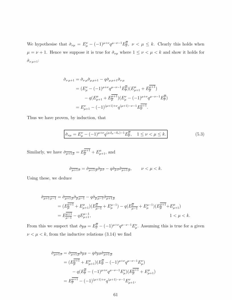
We hypothesise that σνµ = Eνµ − (−1)µ+νqµ−ν−1Eµ

ν , ν < µ ≤ k. Clearly this holds when

µ = ν + 1. Hence we suppose it is true for σνµ where 1 ≤ ν < µ < k and show it holds for

σν µ+1:

σν µ+1 = σν µσµ µ+1 − qσµ µ+1σν µ

= (Eνµ − (−1)µ+νqµ−ν−1Eµ

ν )(Eµµ+1 + Eµ+1

µ )

− q(Eµµ+1 + Eµ+1

µ )(Eνµ − (−1)µ+νqµ−ν−1Eµ

ν )

= Eνµ+1 − (−1)(µ+1)+νq(µ+1)−ν−1Eµ+1

ν .

Thus we have proven, by induction, that

σνµ = Eνµ − (−1)µ+νq(ρ,δµ−δν)−1Eµ

ν , 1 ≤ ν < µ ≤ k. (5.3)

Similarly, we have σµ+1 µ = Eµ+1µ + Eµ

µ+1, and

σµ+1 ν = σµ+1 µσµ ν − qσµ ν σµ+1 µ, ν < µ < k.

Using these, we deduce

σµ+1 µ−1 = σµ+1 µσµ µ−1 − qσµ µ−1σµ+1 µ

= (Eµ+1µ + Eµ

µ+1)(Eµ

µ−1+ Eµ−1

µ ) − q(Eµ

µ−1+ Eµ−1

µ )(Eµ+1µ +Eµ

µ+1)

= Eµ+1

µ−1− qEµ−1

µ+1 , 1 < µ < k.

From this we suspect that σµ ν = Eµν − (−1)µ+νqµ−ν−1Eν

µ. Assuming this is true for a given

ν < µ < k, from the inductive relations (3.14) we find

σµ+1 ν = σµ+1 µσµ ν − qσµ ν σµ+1 µ

= (Eµ+1µ + Eµ

µ+1)(Eµν − (−1)µ+νqµ−ν−1Eν

µ)

− q(Eµν − (−1)µ+νqµ−ν−1Eν

µ)(Eµ+1µ + Eµ

µ+1)

= Eµ+1ν − (−1)(µ+1)+νq(µ+1)−ν−1Eν

µ+1,

61

as expected. Therefore it follows by induction that

σµ ν = Eµν − (−1)µ+νq(ρ,δν−δµ)−1Eν

µ, 1 ≤ ν < µ ≤ k. (5.4)

5.4 Calculating σµi, σi µ

The next step is to find the odd unknowns of the form σµi and σi µ. The process is simplified

by using the values of σba already calculated.

In the case of σµi we first use σν=k i=1 and σµν to find the general σµ i=1 and then apply σji

to extend this to all values of σµi.

Earlier in the chapter we showed that:

σν=k i=1 = Eν=ki=1 + (−1)kqEi=1

ν=k,

σµν = Eµν − (−1)ν+µqν−µ−1Eν

µ, µ < ν ≤ k,

σji = Eji − qj−i+1Ei

j, 1 ≤ j < i ≤ l,

σj l+1 = Ejl+1 − qj−l− 1

2El+1j, 1 ≤ j ≤ l, m = 2l + 1.

The relations we apply are

σµ i=1 = σµ ν=kσν=k i=1 − qσν=k i=1σµ ν=k, µ < k,

σµi = σµ j=1σj=1 i − q−1σj=1 iσµ j=1, i > 1.

Note the second of these is taken from the general form of the inductive relations. Although

one could calculate σµi using only the relations in Tables A.1, A.2 and A.3, at this point

using the general form saves time.

Combining the information, we see

62

σµ i=1 = σµ ν=kσν=k i=1 − qσν=k i=1σµ ν=k, µ < k

= (Eµν=k − (−1)k+µqk−µ−1Eν=k

µ )(Eν=ki=1 + (−1)kqEi=1

ν=k)

− q(Eν=ki=1 + (−1)kqEi=1

ν=k)(Eµ

ν=k − (−1)k+µqk−µ−1Eν=kµ )

= Eµi=1 + (−1)µqk−µ+1Ei=1

µ , µ ≤ k.

63

Then for i ≤ l

σµi = σµ j=1σj=1 i − q−1σj=1 iσµ j=1, 1 < i ≤ l

= (Eµj=1 + (−1)µqk−µ+1Ej=1

µ )(Ej=1i − q2−iEi

j=1)

− q−1(Ej=1i − q2−iEi

j=1)(Eµj=1 + (−1)µqk−µ+1Ej=1

µ )

= Eµi + (−1)µqk−µ+2−iEi

µ, 1 ≤ i ≤ l

= Eµi + (−1)µq(ρ,εi−δµ)+1Ei

µ, 1 ≤ i ≤ l.

It only remains to calculate σµ l+1 when m = 2l + 1. We find

σµ l+1 = σµ i=1σi=1 l+1 − q−1σi=1 l+1σµ i=1

= (Eµi=1 + (−1)µqk−µ+1Ei=1

µ )(Ei=1l+1 − q

12−lEl+1

i=1)

− q−1(Ei=1l+1 − q

12−lEl+1

i=1)(Eµ

i=1 + (−1)µqk−µ+1Ei=1µ )

= Eµl+1 + (−1)µqk−µ−l+ 1

2El+1µ

= Eµl+1 + (−1)µq(ρ,εl+1−δµ)El+1

µ .

Thus

σµi = Eµi + (−1)µq(ρ,εi−δµ)+(εi,εi)Ei

µ, 1 ≤ i ≤ ⌈m2⌉, 1 ≤ µ ≤ k. (5.5)

To find σiµ we follow the same procedure. The known values for σba and recurrence relations

we use are:

64

σi=1 ν=k = Ei=1ν=k

+ (−1)kq−1Eν=ki=1 ,

σν µ = Eνµ − (−1)ν+µqν−µ−1Eµ

ν , 1 ≤ µ < ν ≤ k,

σi j = Eij− qj−i+1Ej

i , 1 ≤ j < i ≤ l,

σl+1 j = El+1j

− qj−1+ 12Ej

l+1, 1 ≤ j ≤ l, m = 2l + 1,

σi=1 µ = σi=1 ν=kσν=k µ − qσν=k µσi=1 ν=k, µ < k,

σi µ = σi j=1σj=1 µ − qσj=1 µσi j=1, i > 1.

From these we determine

σi=1 µ = σi=1 ν=kσν=k µ − qσν=k µσi=1 ν=k, µ < k

= (Ei=1ν=k

+ (−1)kq−1Eν=ki=1 )(Eν=k

µ − (−1)k+µqk−µ−1Eµν=k)

− q(Eν=kµ − (−1)k+µqk−µ−1Eµ

ν=k)(Ei=1ν=k

+ (−1)kq−1Eν=ki=1 )

= Ei=1µ + (−1)µqk−µ−1Eµ

i=1, µ ≤ k.

Therefore, for 1 ≤ µ ≤ k, we find

σi µ = σi j=1σj=1 µ − q−1σj=1µσi j=1, 1 < i ≤ l

= (Eij=1

− q2−iEj=1i )(Ej=1

µ + (−1)µqk−µ−1Eµj=1)

− q−1(Ej=1µ + (−1)µqk−µ−1Eµ

j=1)(Eij=1

− q2−iEj=1i )

= Eiµ + (−1)µqk−µ−iEµ

i , 1 ≤ i ≤ l

and

σl+1 µ = σl+1 j=1σj=1 µ − q−1σj=1 µσl+1 j=1

= (El+1j=1

− q32−lEj=1

l+1 )(Ej=1µ + (−1)µqk−µ−1Eµ

j=1)

− q−1(Ej=1µ + (−1)µqk−µ−1Eµ

j=1)(El+1j=1

− q32−lEj=1

l+1 )

= El+1µ + (−1)µqk−µ−l− 1

2Eµl+1.

65

Hence

σi µ = Eiµ + (−1)µq(ρ,δµ−εi)−1Eµ

i , 1 ≤ i ≤ ⌈m2⌉, 1 ≤ µ ≤ k. (5.6)

5.5 Calculating σi j

Now we construct the operators of the form σi j, starting from the fundamental values asso-

ciated with the root αl. As we currently have different operators depending on the parity of

m, the first step is to unify the two cases.

It has already been shown that when m is even, σl l = 0, σl−1 l = El−1

l− El

l−1and σl l−1 =

Ell−1

−El−1l

. We now calculate those operators for the case m = 2l+1, using the expressions

for σl l+1 and σl+1 l in Table 5.1 together with those for σl−1 l+1 and σl+1 l−1 as determined in

Section 5.2. From the inductive relations (3.14) we find

σl l = qσl l+1σl+1 l − σl+1 lσl l+1

= q(Ell+1 − q−

12El+1

l)(El+1

l− q

12El

l+1) − (El+1

l− q

12El

l+1)(Ell+1 − q−

12El+1

l)

= qEll− El

l.

Also,

σl−1 l = σl−1 l+1σl+1 l − σl+1 lσl−1 l+1

= (El−1l+1 − q−

32El+1

l−1)(El+1

l− q

12El

l+1) − (El+1l

− q12El

l+1)(El−1l+1 − q−

32El+1

l−1)

= El−1

l− q−1El

l−1

and

σl l−1 = σl l+1σl+1 l−1 − σl+1 l−1σl l+1

= (Ell+1 − q−

12El+1

l)(El+1

l−1− q−

12El−1

l+1) − (El+1

l−1− q−

12El−1

l+1)(Ell+1 − q−

12El+1

l)

= Ell−1

− q−1El−1

l.

66

Hence we can say that for both odd and even m,

σl l = qEll− q2l−m+1El

l,

σl−1 l = El−1

l− q2l−mEl

l−1,

σl l−1 = Ell−1

− q2l−mEl−1

l.

Now that we have a formula for σl l and σl−1 l that hold for any m, we can use the general

form of the inductive relations to calculate the remaining values of σij . First we find σil for

all i < l, remembering that

σji = Eji − qj−i+1Ei

j, 1 ≤ j < i ≤ l.

Then

σil = σi l−1σl−1 l − q−1σl−1 lσi l−1, i < l − 1

= (Eil−1 − qi−l+2El−1

i)(El−1

l− q2l−mEl

l−1)

− q−1(El−1

l− q2l−mEl

l−1)(Ei

l−1 − qi−l+2El−1i

)

= Eil− qi+l−m+1El

i, i ≤ l − 1.

Similarly,

σlj = σl l−1σl−1 j − q−1σl−1 j σl l−1, j < l − 1

= (Ell−1

− q2l−mEl−1

l)(El−1

j− qj−l+2Ej

l−1)

− q−1(El−1j

− qj−l+2Ejl−1)(E

ll−1

− q2l−mEl−1

l)

= Elj− qj+l−m+1Ej

l, j ≤ l − 1.

Now we evaluate the remaining operators of the form σij , using the formula for σi j derived

in Section 5.2 together with σil. We find

67

σij = q−(εi,εj)σilσl j − q−1σl j σil, i, j < l

= q−(εi,εj)(Ei

l− qi+l−m+1El

i)(El

j− qj−l+1Ej

l )

− q−1(Elj− qj−l+1Ej

l )(Eil− qi+l−m+1El

i)

= q−(εi,εj)Ei

j− qi+j−m+1Ej

i, i, j ≤ l.

Hence we have shown

σi j = q−(εi,εj)Eij− q(ρ,εj−εi)+1Ej

i, 1 ≤ i, j ≤ l. (5.7)

5.6 Calculating σi µ, σµ i

Next we construct the remaining odd operators, σi µ and σµ i. These are easily calculated

from the operators derived earlier. We simply combine our previous results for σi j and σj µ,

using the unified form of the relations (3.14). They tell us that for any j 6= i, 1 ≤ i, j ≤

l, 1 ≤ µ ≤ k,

σi µ = σi j σj µ − q−1σj µσi j .

Substituting in the values found in Sections 5.4 and 5.5, we find

σi µ = (Eij− qi+j−m+1Ej

i)(Ej

µ + (−1)µqk−µ−jEµj )

− q−1(Ejµ + (−1)µqk−µ−jEµ

j )(Eij− qi+j−m+1Ej

i)

= Eiµ + (−1)µqi−m+k−µEµ

i.

Similarly, for any j 6= i, 1 ≤ i ≤ l, 1 ≤ µ ≤ k we obtain

68

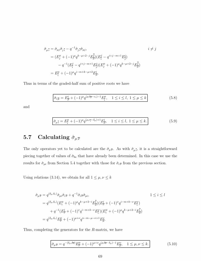
σµ i = σµj σj i − q−1σj iσµj , i 6= j

= (Eµj + (−1)µqk−µ+2−jEj

µ)(Ej

i− qi+j−m+1Ei

j)

− q−1(Ej

i− qi+j−m+1Ei

j)(Eµ

j + (−1)µqk−µ+2−jEjµ)

= Eµ

i+ (−1)µqi−m+k−µ+2Ei

µ.

Thus in terms of the graded-half sum of positive roots we have

σi µ = Eiµ + (−1)µq(ρ,δµ−εi)−1Eµ

i, 1 ≤ i ≤ l, 1 ≤ µ ≤ k (5.8)

and

σµ i = Eµ

i+ (−1)µq(ρ,ε

i−δµ)+1Ei

µ, 1 ≤ i ≤ l, 1 ≤ µ ≤ k. (5.9)

5.7 Calculating σµ ν

The only operators yet to be calculated are the σµ ν . As with σµ i, it is a straightforward

piecing together of values of σba that have already been determined. In this case we use the

results for σµi from Section 5.4 together with those for σi ν from the previous section.

Using relations (3.14), we obtain for all 1 ≤ µ, ν ≤ k

σµ ν = q(δµ,δν)σµiσi ν + q−1σi ν σµi, 1 ≤ i ≤ l

= q(δµ,δν)(Eµi + (−1)µqk−µ+2−iEi

µ)(Eiν + (−1)νqi−m+k−νEν

i)

+ q−1(Eiν + (−1)νqi−m+k−νEν

i)(Eµ

i + (−1)µqk−µ+2−iEiµ)

= q(δµ,δν)Eµν + (−1)µ+νqn−m−µ−ν+1Eν

µ.

Thus, completing the generators for the R-matrix, we have

σµ ν = q−(δµ,δν)Eµν + (−1)µ+νq(ρ,δν−δµ)−1Eν

µ, 1 ≤ µ, ν ≤ k. (5.10)

69

5.8 Solution for the R-matrix in the Vector Represen-

tation.

In this chapter we have calculated the explicit solution for all the σba, εb > εa, in the vector

representation, which form the basis for the R-matrix. Looking over equations (5.1) through

to (5.10) we can see a general form for σba, namely

σba = q−(εa,εb)Eba − (−1)[b]([a]+[b])ξaξbq

(εa,εa)q(ρ,εa−εb)Eab, εb > εa.

Thus we have shown the R-matrix for the vector representation of Uq[osp(m|n)], R = (π ⊗

π)R, is given by

R = qhj⊗hj[

I ⊗ I + (q − q−1)∑

εb>εa


]

where

σba = q−(εa,εb)Eba − (−1)[b]([a]+[b])ξaξbq

(εa,εa)q(ρ,εa−εb)Eab.

This can be written in a more elegant form. Recall that the ansatz for R can also be written

as

R =∑

a


∑

εb>εa

(−1)[b]Eab ⊗ qhεa σba.

In the vector representation, this is equal to

R =∑

a,b

q(εa,εb)Eaa ⊗Eb

b + (q − q−1)∑

εb>εa


in terms of generators

σba = qhεa σba

= Eba − (−1)[b]([a]+[b])ξaξbq

(ρ,εa−εb)Eab.

70

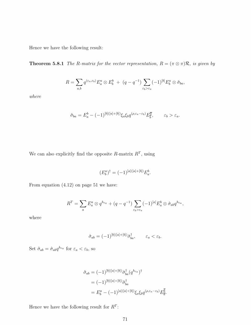
Hence we have the following result:

Theorem 5.8.1 The R-matrix for the vector representation, R = (π ⊗ π)R, is given by

R =∑

a,b

q(εa,εb)Eaa ⊗ Eb

b + (q − q−1)∑

εb>εa

(−1)[b]Eab ⊗ σba,

where

σba = Eba − (−1)[b]([a]+[b])ξaξbq

(ρ,εa−εb)Eab, εb > εa.

We can also explicitly find the opposite R-matrix RT , using

(Eab )† = (−1)[a]([a]+[b])Eb

a.

From equation (4.12) on page 51 we have:

RT =∑

a


∑

εb>εa

(−1)[a]Eba ⊗ σabq

hεa ,

where

σab = (−1)[b]([a]+[b])σ†ba, εa < εb.

Set σab = σabqhεa for εa < εb, so

σab = (−1)[b]([a]+[b])σ†ba(q

hεa )†

= (−1)[b]([a]+[b])σ†ba

= Eab − (−1)[a]([a]+[b])ξaξbq

(ρ,εa−εb)Eba.

Hence we have the following result for RT :

71

Theorem 5.8.2 The opposite R-matrix for the vector representation,

RT = (π ⊗ π)RT , is given by

RT =∑

a,b

q(εa,εb)Eaa ⊗Eb

b + (q − q−1)∑

εb>εa

(−1)[a]Eba ⊗ σab,

where

σab = Eab − (−1)[a]([a]+[b])ξaξbq

(ρ,εa−εb)Eba.

These formulae for R and RT on the vector representation agree with those given in [36].

In that thesis the R-matrix for the vector representation was calculated using projection

operators onto invariant submodules of the tensor product. The greatest advantage of the

current method is it gives a straightforward way of constructing a solution to the Yang-Baxter

Equation in an arbitrary representation of Uq[osp(m|n)].

72

Chapter 6

Casimir Invariants and their

Eigenvalues

The Lax operator can be used not only to construct solutions of the quantum Yang-Baxter

Equation, but also to find families of Casimir invariants. These are an important tool for

understanding the representation theory of the superalgebra. After constructing the Casimir

invariants we can use properties of the root system to calculate their eigenvalues when acting

on an irreducible highest weight module.

In this chapter we do exactly that, basing our method upon that used in [4] and [43] for

the classical general and orthosymplectic superalgebras respectively. This was adapted in

[33] to cover the quantum superalgebra Uq[gl(m|n)]. Although the concepts are much the

same as in those cases, the combination of the q-deformation and the more complex root

system of Uq[osp(m|n)] makes the calculations in this chapter substantially more technically

challenging.

6.1 Casimir Invariants of Uq[osp(m|n)]

Before constructing the Casimir invariants we need to define a new object. Let hρ be the

unique element of the Cartan subalgebra H satisfying

73

αi(hρ) = (ρ, αi), ∀αi ∈ H∗.

It is also convenient to define a new operator ∂ by

∂ ≡ (π ⊗ id)∆.

Then from [53] we have the following theorem:

Theorem 6.1.1 Let V be the representation space of π, an arbitrary finite dimensional

representation of Uq[osp(m|n)]. If Γ ∈ (End V ) ⊗ Uq[osp(m|n)] satisfies

∂(a)Γ = Γ∂(a), ∀a ∈ Uq[osp(m|n)], (6.1)

then

C = (str ⊗ id)(π(q2hρ) ⊗ I)Γ

belongs to the centre of Uq[osp(m|n)]. Above str denotes the supertrace.

Now choose π to be the vector representation. Recalling that an R-matrix satisfies

R∆(a) = ∆T (a)R, ∀a ∈ Uq[osp(m|n)],

it is clear that

∂(a)RTR = RTR∂(a), ∀a ∈ Uq[osp(m|n)].

Hence if we set A ∈ (End V ) ⊗ Uq[osp(m|n)] to be

A =(RTR− I ⊗ I)

(q − q−1),

the operators Al will satisfy condition (6.1) for all non-negative integers l. Thus the operators

Cl defined as

74

Cl = (str ⊗ id)(π(q2hp) ⊗ I)Al, l ∈ Z+,

form a family of Casimir invariants. Here A coincides with the matrix of Jarvis and Green [24]

in the classical limit q → 1, as do the invariants Cl.

Now write the Lax operator R and its opposite RT in the form

R = I ⊗ I + (q − q−1)∑

εb≥εa

Eab ⊗Xb

a,

RT = I ⊗ I + (q − q−1)∑

εb≤εa

Eab ⊗Xb

a.

In terms of the operators σba, this implies

Xba =

qhεa−I

q−q−1 , a = b,

(−1)[b]qhεa σba, εa < εb,

(−1)[b]σbaqhεb , εa > εb.

Writing A as

A =∑

a,b

Eab ⊗ Ab

a,

we obtain

Aba = (1 + δa

b )Xba + (q − q−1)

∑

εc≤εa,εb

(−1)([a]+[c])([b]+[c])XcaX

bc .

This produces a family of Casimir invariants

Cl =∑

a

(−1)[a]q(2ρ,εa)A(l)a

a,

where the operators A(l)b

a are recursively defined as

A(l)b

a =∑

c

(−1)([a]+[c])([b]+[c])A(l−1)c

aAbc. (6.2)

75

6.2 Setting up the Eigenvalue Calculations

Now that we have found a family of Casimir invariants, we wish to calculate their eigenvalues

on a general irreducible finite-dimensional module. Let V (Λ) be an arbitrary irreducible

finite-dimensional module with highest weight Λ and highest weight state |Λ〉. Define t(l)a to

be the eigenvalue of A(l)a

a on this state, so

A(l)a

a|Λ〉 = t(l)a |Λ〉.

Once we have calculated t(l)a we will use the result to find the eigenvalues of the Casimir

invariants Cl.

To evaluate t(l)a , note that if εb > εa then A(l)b

a is a raising operator, implying A(l)b

a|Λ〉 = 0.

Thus from equation (6.2) we deduce

t(l)a |Λ〉 = t(l−1)a t(1)a |Λ〉 +

∑

εa<εb

(−1)[a]+[b]A(l−1)b

aAab |Λ〉

= t(l−1)a t(1)a |Λ〉 +

∑

εa<εb

(−1)[a]+[b]A(l−1)b

a

[

Xab + (q − q−1)Xa

bXaa

]

|Λ〉

= t(l−1)a t(1)a |Λ〉 +

∑

εa<εb

(−1)[a]+[b]q(Λ,εa)A(l−1)b

aXab |Λ〉.

Now we know that

Al∂(Xab ) = ∂(Xa

b )Al. (6.3)

This can be used to calculate A(l)b

aXab |Λ〉 for εa < εb. First we need an expression for ∆(Xa

b ).

The R-matrix properties give

(∆ ⊗ I)R = R13R23

⇒ (I ⊗ ∆)RT = RT12R

T13.

In terms of Xab , this implies

76

I ⊗ I ⊗ I+(q − q−1)∑

εa≤εb

Eba ⊗ ∆(Xa

b )

=(

I ⊗ I ⊗ I + (q − q−1)∑

εa≤εb

Eba ⊗Xa

b ⊗ I)

×(

I ⊗ I ⊗ I + (q − q−1)∑

εa≤εb

Eba ⊗ I ⊗Xa

b

)

= I ⊗ I ⊗ I + (q − q−1)∑

εa≤εb

Eba ⊗ (Xa

b ⊗ I + I ⊗Xab )

+ (q − q−1)2∑

εa≤εc≤εb

(−1)([a]+[c])([b]+[c])Eba ⊗Xc

b ⊗Xac .

Hence for all εa < εb

∆(Xab ) = Xa

b ⊗ I + I ⊗Xab + (q − q−1)

∑

εa≤εc≤εb

(−1)([a]+[c])([b]+[c])Xcb ⊗Xa

c .

We also need an expression for π(Xab ) for εa ≤ εb. At the end of the previous chapter we

found that the generators for RT in the vector representation are given by

σab = σabqhεa = Ea

b − (−1)[a]([a]+[b])ξaξbq(ρ,εa−εb)Eb

a, εa < εb.

From this we deduce that

π(Xab ) = (−1)[a]π(σabq

hεa )

= (−1)[a]Eab − (−1)[a][b]ξaξbq

(ρ,εa−εb)Eba, εa < εb.

Also, we know

π(Xaa ) = (q − q−1)−1π(qhεa − I)

= (q − q−1)−1(q(εa,εa)(Eaa−Ea

a) − I).

Applying these, we find that if εa < εb then

77

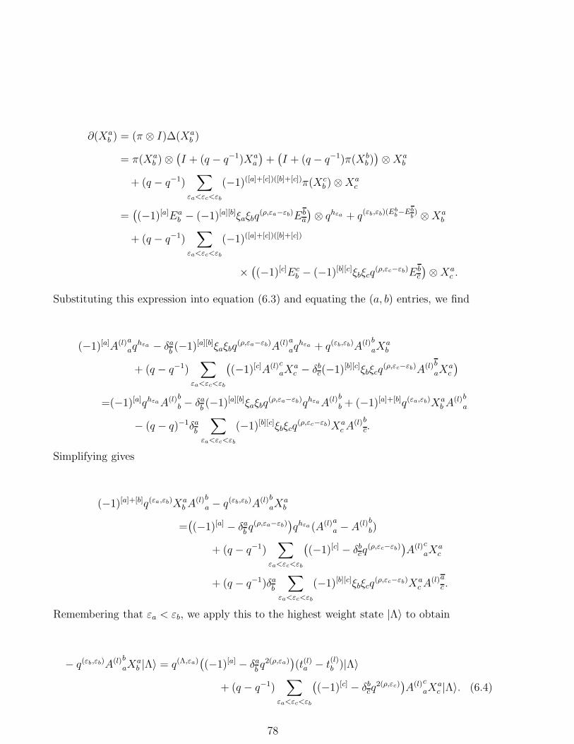
∂(Xab ) = (π ⊗ I)∆(Xa

b )

= π(Xab ) ⊗

(

I + (q − q−1)Xaa

)

+(

I + (q − q−1)π(Xbb )

)

⊗Xab

+ (q − q−1)∑

εa<εc<εb

(−1)([a]+[c])([b]+[c])π(Xcb ) ⊗Xa

c

=(

(−1)[a]Eab − (−1)[a][b]ξaξbq

(ρ,εa−εb)Eba

)

⊗ qhεa + q(εb,εb)(Ebb−Eb

b) ⊗Xa

b

+ (q − q−1)∑

εa<εc<εb

(−1)([a]+[c])([b]+[c])

×(

(−1)[c]Ecb − (−1)[b][c]ξbξcq

(ρ,εc−εb)Ebc

)

⊗Xac .

Substituting this expression into equation (6.3) and equating the (a, b) entries, we find

(−1)[a]A(l)a

aqhεa − δa

b(−1)[a][b]ξaξbq

(ρ,εa−εb)A(l)a

aqhεa + q(εb,εb)A(l)b

aXab

+ (q − q−1)∑

εa<εc<εb

(

(−1)[c]A(l)c

aXac − δb

c(−1)[b][c]ξbξcq(ρ,εc−εb)A(l)b

aXac

)

=(−1)[a]qhεaA(l)b

b − δab(−1)[a][b]ξaξbq

(ρ,εa−εb)qhεaA(l)b

b + (−1)[a]+[b]q(εa,εb)XabA

(l)b

a

− (q − q)−1δab

∑

εa<εc<εb

(−1)[b][c]ξbξcq(ρ,εc−εb)Xa

cA(l)b

c.

Simplifying gives

(−1)[a]+[b]q(εa,εb)XabA

(l)b

a − q(εb,εb)A(l)b

aXab

=(

(−1)[a] − δabq(ρ,εa−εb)

)

qhεa (A(l)a

a −A(l)b

b)

+ (q − q−1)∑

εa<εc<εb

(

(−1)[c] − δbcq

(ρ,εc−εb))

A(l)c

aXac

+ (q − q−1)δab

∑

εa<εc<εb

(−1)[b][c]ξbξcq(ρ,εc−εb)Xa

cA(l)a

c .

Remembering that εa < εb, we apply this to the highest weight state |Λ〉 to obtain

− q(εb,εb)A(l)b

aXab |Λ〉 = q(Λ,εa)

(

(−1)[a] − δabq2(ρ,εa)

)

(t(l)a − t(l)b )|Λ〉

+ (q − q−1)∑

εa<εc<εb

(

(−1)[c] − δbcq

2(ρ,εc))

A(l)c

aXac |Λ〉. (6.4)

78

The next step is to calculate A(l)b

aXab |Λ〉 for εa < εb. It is first convenient to order the indices

according to b > c ⇔ εb < εc. With this ordering we say an element a > 0 if εa < 0, a = 0

if εa = 0, and a < 0 if εa > 0. Using this convention, it is apparent the solution to (6.4) will

be of the form

A(l)b

aXab |Λ〉 = q(Λ,εa)(−1)[a]

∑

a>c≥b

αabc(t

(l)a − t(l)c )|Λ〉, (6.5)

where αabc is a function of a, b and c. Now from equation (6.4) we have

(q − q−1)∑

a>c>b

(−1)[c]A(l)c

aXac |Λ〉

= −q(εb,εb)A(l)b

aXab |Λ〉 + (q − q−1)

∑

a>c>b

δbcq

−2(ρ,εb)A(l)c

aXac |Λ〉

− (−1)[a]q(Λ,εa)(

1 − δab(−1)[a]q2(ρ,εa)

)

(t(l)a − t(l)b )|Λ〉

= −q(εb+1,εb+1)A(l)b+1

a Xab+1|Λ〉

+ (q − q−1)∑

a>c>b+1

δb+1c q−2(ρ,εb+1)A(l)c

aXac |Λ〉

− (−1)[a]q(Λ,εa)(

1 − δb+1a (−1)[a]q2(ρ,εa)

)

(t(l)a − t(l)b+1)|Λ〉

+ (q − q−1)(−1)[b+1]A(l)b+1

a Xab+1|Λ〉.

Substituting in the form of the solution given in equation (6.5) produces

q(εb,εb)∑

a>d≥b

αabd(t

(l)a − t

(l)d )|Λ〉

=(

q(εb+1,εb+1) − (q − q−1)(−1)[b+1])

∑

a>d≥b+1

αab+1 d(t

(l)a − t

(l)d )|Λ〉

−(

1 − δab(−1)[a]q2(ρ,εa)

)

(t(l)a − t(l)b )|Λ〉 +

(

1 − δab+1

(−1)[a]q2(ρ,εa))

(t(l)a − t(l)b+1)|Λ〉

+(q − q−1)∑

a>c>b

δbcq

−2(ρ,εb)∑

a>d≥c

αab d

(t(l)a − t(l)d )|Λ〉

−(q − q−1)∑

a>c>b+1

δb+1c q−2(ρ,εb+1)

∑

a>d≥c

αab+1 d

(t(l)a − t(l)d )|Λ〉. (6.6)

79

Set

αabd = αbd(1 − δa

d(−1)[a]q2(ρ,εa)).

Then from equation (6.6) we obtain

αbb = −q−(εb,εb)

and

αb b+1 = q−(εb,εb)[

(

q(εb+1,εb+1) − (q − q−1)(−1)[b+1])

αb+1 b+1 + 1

+ (q − q−1)δbb+1q−2(ρ,εb)αb b+1

]

= q−(εb,εb)[

(

(q − q−1)(−1)[b+1] − q(εb+1,εb+1))

q−(εb+1,εb+1) + 1

− (q − q−1)δbb+1q−2(ρ,εb)q−(εb+1,εb+1)

]

= q−(εb,εb)−(εb+1,εb+1)(q − q−1)(

(−1)[b+1] − δbb+1q−2(ρ,εb)

)

.

To simplify this expression note that q2(ρ,εb+1−εb) = q−(εb,εb)−(εb+1,εb+1) in all cases except for

[b] = 0, b = l, m = 2l, in which case q2(ρ,εb+1−εb) = q2q−(εb,εb)−(εb+1,εb+1). However [b] = 0, b =

l, m = 2l if and only if δbb+1

= 1, and in that case we find αb b+1 = 0. Hence for all values of

b we can write

αb b+1 = (q − q−1)q−2(ρ,εb)(

(−1)[b+1]q2(ρ,εb+1) − δbb+1

)

.

Now that we have found αbb and αb b+1, they can be used to calculate the remaining αbd.

From equation (6.6) we observe that if d > b+ 1 then

αbd = q−(εb,εb)(

q(εb+1,εb+1) − (q − q−1)(−1)[b+1])

αb+1 d

+ (q − q−1)q−(εb,εb)∑

d≥c>b

δbcq

−2(ρ,εb)αbd

− (q − q−1)q−(εb,εb)∑

d≥c>b+1

δb+1c q−2(ρ,εb+1)αb+1d.

80

Remembering that θxy was defined by

θxy =

1 x < y,

0 x ≥ y,

this can be rewritten as


q(εb+1,εb+1) − (q − q−1)(−1)[b+1])

αb+1 d

+ (q − q−1)q−(εb,εb)q2(ρ,εc)(

θbcθc d+1δbc − θb+1 cθc d+1δ

b+1c

)

αcd, d > a+ 1. (6.7)

Now consider αbd for any b > l. Both θbb and θb+1 b+1 will equal 0, so


q(εb+1,εb+1) − (q − q−1)(−1)[b+1])

αab+1 d

= q−(εb,εb)q−(εb+1,εb+1)αb+1 d

= q2(ρ,εb+1−εb)αb+1 d.

Since

αd−1 d = (−1)[d](q − q−1)q2(ρ,εd−εd−1),

we obtain

αbd = (−1)[d](q − q−1)q2(ρ,εd−εb), d > b > l.

Substituting this together with our expression for αbb into equation (6.7), we find

αbd =q−(εb,εb)(

q−(εb+1,εb+1) − δb+1

b+1(q − q−1)

)

αb+1 d

+(q − q−1)2q−(εb,εb)(−1)[d]q2(ρ,εd)(

θbbθbd − θb+1 b+1θb+1d

)

−(q − q−1)q−(εb,εb)q−(εd,εd)q2(ρ,εd)(δbd − δb+1

d ), d > b+ 1. (6.8)

81

But for d > b+ 1

θbbθbd − θb+1 b+1θb+1 d = δbl θld − δb

dθbl

= δbl (1 − δd

l) − δb

d(1 − δbl )

= δbl − δb

d.

Also, −[(−1)[d](q − q−1) + q−(εd,εd)]δbd = −q(εd,εd)δb

d, so equation (6.8) reduces to

αbd =(

q2(ρ,εb+1−εb)q−2δb

b+1 − δb+1

b+1q−1(q − q−1)

)

αb+1 d + δbl q

−1(q − q−1)2(−1)[d]q2(ρ,εd)

− δbd(q − q−1)q2(ρ,εd) + δb+1

d (q − q−1)q2(ρ,εb+1−εb)q−2δb

b+1q2(ρ,εd)

=(


b+1 − δb+1

b+1q−1(q − q−1)

)

αb+1 d + δbl q

−1(q − q−1)2(−1)[d]q2(ρ,εd)

+ (q − q−1)q−2(ρ,εb)(δb+1d − δb

d), d > b+ 1.

Recall that for b > l we have

αbd = (−1)[d](q − q−1)q2(ρ,εd−εb), d > b.

Then when b = l we find

αbd =(


b+1 − δb+1

b+1q−1(q − q−1)

)

(−1)[d](q − q−1)q2(ρ,εd−εb+1)

+ q−1(q − q−1)2(−1)[d]q2(ρ,εd) − (q − q−1)q−2(ρ,εb)δld

= (−1)[d](q − q−1)q2(ρ,εd−εb)

[

δb+1

b+1

(

1 − (q − q−1) + (q − q−1))

+ δbb+1

(

q−2 + q−1(q − q−1)]

− (q − q−1)q−2(ρ,εb)δld

= (q − q−1)q−2(ρ,εb)(

(−1)[d]q2(ρ,εd) − δbd

)

for all d > b+ 1. Comparing this with our earlier results for d = b+ 1 and b > l, we have

αbd = (q − q−1)q−2(ρ,εb)(

(−1)[d]q2(ρ,εd) − δbd

)

, ∀b ≥ l, d > b.

82

But for b < l we know

αbd = q2(ρ,εb+1−εb)αb+1 d + (q − q−1)q−2(ρ,εb)(δb+1d − δb

d), d > b+ 1.

Hence for all b we obtain

αbd = (q − q−1)q−2(ρ,εb)(

(−1)[d]q2(ρ,εd) −d−1∑

c=b

δcd +

d−2∑

c=b

δc+1d

)

= (q − q−1)q−2(ρ,εb)(

(−1)[d]q2(ρ,εd) − δbd

)

, d > b.

Thus for all a > b

A(l)b

aXab |Λ〉 = q(Λ,εa)(−1)[a]

∑

a>c≥b

αabc(t

(l)a − t(l)c )|Λ〉,

where αabc is given by

αabc =

−q−(εb,εb)(1 − δab(−1)[a]q2(ρ,εa)), c = b,

(q − q−1)q−2(ρ,εb)(

(−1)[c]q2(ρ,εc) − δbc

)

(1 − δac (−1)[a]q2(ρ,εa)), c > b.

6.3 Constructing the Perelomov-Popov

Matrix Equation

This expression can now be substituted into the equation

t(l)a |Λ〉 = t(l−1)a t(1)a |Λ〉 +

∑

εa<εb

(−1)[a]+[b]q(Λ,εa)A(l−1)b

aXab |Λ〉

to find a matrix equation for the various t(l)a . The matrix factor is an analogue of the

Perelomov-Popov matrix introduced in [40] and [41], which has been used to calculate the

eigenvalues of the Casimir invariants of various classical Lie algebras.

First recall that

83

Aba = (1 + δa

b )Xba + (q − q−1)

∑

c≥a,b

(−1)([a]+[c])([b]+[c])XcaX

bc ,

where

Xba =

qhεa−I

q−q−1 , a = b,

(−1)[b]qhεa σba, εa < εb,

(−1)[b]σbaqhεb , εa > εb.

Then

Aaa|Λ〉 = 2Xa

a |Λ〉 + (q − q−1)XaaX

aa |Λ〉

= (q − q−1)−1(2(qhεa − 1) + (qhεa − 1)2)|Λ〉.

∴ t(1)a =q2(Λ,εa) − 1

q − q−1.

Hence we obtain

t(l)a =(q2(Λ,εa) − 1)

(q − q−1)t(l−1)a

+∑

b<a

(−1)[a]+[b]q(Λ,εa)(

q(Λ,εa)(−1)[a]∑

b≤c<a

αabc(t

(l−1)a − t(l−1)

c ))

=(q2(Λ,εa) − 1)

(q − q−1)t(l−1)a

− q2(Λ,εa)∑

b<a

(−1)[b]q−(εb,εb)(1 − δab(−1)[a]q2(ρ,εa))(t(l−1)

a − t(l−1)b )

+ (q − q−1)q2(Λ,εa)∑

c<b<a

(−1)[c]q−2(ρ,εc)(1 − δab(−1)[a]q2(ρ,εa))

((−1)[b]q2(ρ,εb) − δbc)(t

(l−1)a − t

(l−1)b ).

Now consider the function γb defined by:

γb = (−1)[b]q−(εb,εb) − (q − q−1)∑

c<b

(−1)[c]q−2(ρ,εc)(

(−1)[b]q2(ρ,εb) − δbc)

)

.

84

We evaluate this for all b, labelling C(Λ0) = (δ1, δ1 +2ρ) = m−n− 1 and remembering that

ρ =1

2

l∑

i=1

(m− 2i)εi +1

2

k∑

µ=1

(n−m+ 2 − 2µ)δµ.

First we consider the case [b] = 1 and b ≤ k. Here γb is given by

γb = −q − (q − q−1)q−(n−m+2−2b)∑

c<b

qn−m+2−2c

= −q − (q − q−1)(q2 − 1)−1(q2b − q2)

= (−1)[b]q2(ρ,εb)q−C(Λ0).

For [b] = 0, b ≤ l, we obtain

γb = q−1 − (q − q−1)qm−2b[

(q2 − 1)−1(q2−m − qn−m+2) +∑

ε1≥εc>εb

q2c−m]

= q−1 − q−1(q2−2b − qn+2−2b + 1 − q2−2b)

= (−1)[b]q2(ρ,εb)q−C(Λ0).

In the case b = l + 1, m = 2l + 1, we find

γb = 1 − q−1(−qn−m+2 + q2l+2−m)

= (−1)[b]q2(ρ,εb)q−C(Λ0).

If [b] = 0 and b ≥ l then

γb = q−1 − (q − q−1)q2b−m[

(q2 − 1)−1(q2l+2−m − qn−m+2) + (m− 2l) +∑

b>i≥l

qm−2i]

+ (q − q−1)q2(ρ,εb)

= q−1 − q−1q2b−m[

q2l+2−m − qn−m+2 + qm−2b − qm−2l + (m− 2l)(q2 − 1)]

+ (q − q−1)q2b−m

= q−1 − q−1(1 − qn−2m+2+2b) + (q − q−1)(q2b−m − q2b−m)

= (−1)[b]q2(ρ,εb)q−C(Λ0).

85

Lastly, when [b] = 1 and b ≥ k we find

γb = −q + (q − q−1)qn−m+2−2b[

(q2 − 1)−1(qm − qn−m+2 + q2 − 1) −∑

b>c≥k

qm−n−2+2c]

− (q − q−1)qn−m+2−2b

= −q + q−1qn−m+2−2b(qm − qn−m+2 − qm−n+2k + qm−n+2b)

= −q2n−2m+3−2b

= (−1)[b]q2(ρ,εb)q−C(Λ0).

Hence for all b

γb = (−1)[b]q2(ρ,εb)q−C(Λ0).

We also consider the function

βa = 1 − (q − q−1)∑

b<a

γb

(

1 − δab(−1)[a]q2(ρ,εa)

)

,

so that

t(l)a =(q2(Λ,εa)βa − 1)

(q − q−1)t(l−1)a + q2(Λ,εa)

∑

b<a

γb

(

1 − δab(−1)[a]q2(ρ,εa)

)

t(l−1)b . (6.9)

As before, we evaluate this by considering the various cases individually. Firstly, for [a] =

1, a ≤ k we find

βa = 1 + (q − q−1)∑

b<a

q2b−2+m−nqn−m+1

= 1 + q−1(q2a−2+m−n − qm−n)qn−m+1

= q(εa,2ρ+εa)−C(Λ0).

Using this, when [a] = 0 and a ≤ l we obtain

86

βa = q2(k+1)−2 − (q − q−1)∑

ε1≥εb>εa

qm−2bqn−m+1

= qn − q−1qn−m+1(qm − qm−2a+2)


In the case a = l + 1, m = 2l + 1, we find

βa = qm−2(l+1)+1qn−m+1


For the remaining values of a, we consider the cases m = 2l and m = 2l + 1 separately.

Firstly, take m = 2l. Then for [a] = 0, a ≥ l, we obtain

βa = qm−2(l+1)+1q−C(Λ0) + (q − q−1)γaq2(ρ,εa) − (q − q−1)

a−1∑

b=l

q2b−mq−C(Λ0)

= q−C(Λ0)[q−1 + (q − q−1) − q−1(q2l+2−m − q2a+2−m)]

= q(εa,2ρ+εa)−C(Λ0),

whereas for the remaining odd values of a, namely a ≥ k, βa is given by

βa = q−C(Λ0)(

q−1 − q−1(q2 − q2−m))

− (q − q−1)γaq2(ρ,εa)

+ (q − q−1)

a−1∑

b=k

qn−m+2−2bq−C(Λ0)

= q−C(Λ0)[q−1 − q−1(q2 − q2−m) + (q − q−1) + q−1(qn−m+2−2a − q2−m)]


Now consider m = 2l + 1. If [a] = 0 and a > l + 1 then

87

βa = q−C(Λ0) − (q − q−1)q−C(Λ0) + (q − q−1)γaq2(ρ,εa) −

a−1∑

b=l

q2b−mq−C(Λ0)

= q−C(Λ0)[1 − (q − q−1) + (q − q−1) − q−1(q2l+2−m − q2a+2−m)]


For the remaining case of [a] = 1, a ≥ k, we find

βa = q−C(Λ0)[1 − (q − q−1) − q−1(q − q2−m)] − (q − q−1)γaq2(ρ,εa)

+ (q − q−1)a−1∑

b=k

qn−m+2−2bq−C(Λ0)

= q−C(Λ0)[1 − (q − q−1) − q−1(q − q2−m) + (q − q−1) + q−1(qn−m+2−2a − q2−m)]


Hence βa is given by

βa = q(εa,2ρ+εa)−C(Λ0)

for any a, regardless of the parity of m. Substituting this result together with that for γb

into equation (6.9) gives

t(l)a =(q(εa,2Λ+2ρ+εa)−C(Λ0) − 1)

(q − q−1)t(l−1)a

+ q(2Λ,εa)−C(Λ0)∑

b<a

(−1)[b]q(2ρ,εb)(

1 − δab(−1)[a]q(2ρ,εa)

)

t(l−1)b .

This can be written in the matrix form

t(l) = Mt(l−1),

where M is a lower triangular matrix with entries

88

Mab =

0, a < b

(q − q−1)−1(q(εa,2Λ+2ρ+εa)−C(Λ0) − 1), a = b,

q(2Λ,εa)−C(Λ0)(

(−1)[b]q(2ρ,εb) − δab

)

, a > b.

Then we have

t(l) = M lt(0), where t(0)a = 1 ∀a,

where M is an analogue of the Perelomov-Popov matrix.

6.4 Finding the Eigenvalues

This matrix equation for t(l)a can now be used to calculate the eigenvalues of Cl. Loosely

speaking, the problem reduces to diagonalising the matrix M . As with the earlier calcula-

tions, the q-factors from the q-deformation and the δ-functions arising from the root system

make this somewhat more difficult than in the classical cases studied in [4] and [43], and also

than in the case of Uq[gl(m|n)] [33].

Recall

Cl =∑

a

(−1)[a]q(2ρ,εa)A(l)a

a.

Denote the eigenvalue of Cl on V (Λ) as χΛ(Cl). Then we have

χΛ(Cl) =∑

a

(−1)[a]q(2ρ,εa)t(l)a =∑

a,b

(−1)[a]q(2ρ,εa)(M l)ab.

To calculate this we wish to diagonalise M . We assume the eigenvalues of M ,

αΛa =

(q(εa,2Λ+2ρ+εa)−C(Λ0) − 1)

(q − q−1),

are distinct. Then we need a matrix N satisfying

89

(N−1MN)ab = δabα

Λa ,

which implies

χΛ(Cl) =∑

a,b,c

(−1)[a]q(2ρ,εa)(αΛb )lNab(N

−1)bc. (6.10)

Now

(MN)ab = αΛb Nab.

Substituting in the values for Mab gives

αΛaNab + q(2Λ,εa)−C(Λ0)

∑

c<a

(

(−1)[c]q(2ρ,εc) − δac

)

Ncb = αΛb Nab. (6.11)

Since the eigenvalues αΛa are distinct, this implies

Nab = 0, ∀a < b.

Set

Pab =∑

c≤a

(−1)[c]q(2ρ,εc)Ncb. (6.12)

Then equation (6.11) becomes

(αΛb − αΛ

a )Nab = q(2Λ,εa)−C(Λ0)Pa−1 b − θ0aq(2Λ,εa)−C(Λ0)Nab

⇒ (αΛb − αΛ

a )(−1)[a]q(−2ρ,εa)(Pab − Pa−1 b)

= q(2Λ,εa)−C(Λ0)Pa−1 b − θ0aq(2Λ,εa)−C(Λ0)Nab,

which simplifies to

Pab =(αΛ

b − αΛa + (−1)[a]q2(Λ+ρ,εa)−C(Λ0))

(αΛb − αΛ

a )Pa−1 b −

θ0a(−1)[a]q2(Λ+ρ,εa)−C(Λ0)

(αΛb − αΛ

a )Nab.

90

Set

ψba = αΛ

b − αΛa + (−1)[a]q2(Λ+ρ,εa)−C(Λ0),

so this becomes

Pab =ψb

a

(αΛb − αΛ

a )Pa−1 b −

θ0a(−1)[a]q2(Λ+ρ,εa)−C(Λ0)

(αΛb − αΛ

a )Nab. (6.13)

Without loss of generality we can choose Naa = 1 ∀a, so Pbb = (−1)[b]q2(ρ,εb). Then in the

cases 0 ≥ a > b and a > b ≥ 0 the last term in equation (6.13) vanishes, giving

Pab = (−1)[b]q2(ρ,εb)a

∏

c=b+1

ψbc

(αΛb − αΛ

c ).

Similarly, for a > b > 0 we obtain

Pab = Pbb

a∏

c=b+1

ψbc

(αΛb − αΛ

c ). (6.14)

It remains to find Pab for b ≥ a > 0. In this case, the last term in equation (6.13) contributes,

giving

Pab = (−1)[b]q2(ρ,εb)

a∏

c=b+1

ψbc

(αΛb − αΛ

c )−

(−1)[a]q2(Λ+ρ,εa)−C(Λ0)

(αΛb − αΛ

a )Nab

−

a−1∑

j=l

(−1)[j]q2(Λ+ρ,εj)−C(Λ0)

(αΛb − αΛ

j )Njb

a∏

c=j+1

ψbc

(αΛb − αΛ

c ). (6.15)

Recall that if b < a < 0, then

Nab =q(2Λ,εa)−C(Λ0)

(αΛb − αΛ

a )Pa−1 b

=(−1)[b]q2(Λ,εa)+2(ρ,εb)−C(Λ0)

(αΛb − αΛ

a )

a−1∏

c=b+1

ψbc

(αΛb − αΛ

c ).

Substituting this into equation (6.15), we find

91

Pbb = (−1)[b]q2(ρ,εb)b

∏

c=b+1

ψbc

(αΛb − αΛ

c )−

(−1)[b]q−2(Λ+ρ,εb)−C(Λ0)

(αΛb − αΛ

b)

−

b−1∑

j=l

(−1)[j]+[b]q2(ρ,εj+εb)−2C(Λ0)

(αΛb − αΛ

j )(αΛb − αΛ

j)

j−1∏

c=b+1

ψbc

(αΛb − αΛ

c )

b∏

c=j+1

ψbc

(αΛb − αΛ

c ),

which can also be written as

Pbb

b∏

c=b+1

(αΛb − αΛ

c )

ψbc

= (−1)[b]q2(ρ,εb) −(−1)[b]q−2(Λ+ρ,εb)−C(Λ0)

(αΛb − αΛ

b)

b∏

c=b+1

(αΛb − αΛ

c )

ψbc

−

b−1∑

j=l

(−1)[j]+[b]q2(ρ,εb+εj)−2C(Λ0)

(αΛb − αΛ

j )(αΛb − αΛ

j)

j∏

c=j

(αΛb − αΛ

c )

ψbc

= (−1)[b]q2(ρ,εb) −q−2C(Λ0)

ψbbψb

b

b−1∏

c=b+1

(αΛb − αΛ

c )

ψbc

−b−1∑

j=l

(−1)[j]+[b]q2(ρ,εb+εj)−2C(Λ0)

ψbjψ

bj

j−1∏

c=j+1

(αΛb − αΛ

c )

ψbc

= (−1)[b]q2(ρ,εb)

[

1 −b

∑

j=l

(−1)[j]q2(ρ,εj)−2C(Λ0)

ψbjψ

bj

j−1∏

c=j+1

(αΛb − αΛ

c )

ψbc

]

. (6.16)

From this point we will consider the case m = 2l + 1. This is marginally more complicated

than the case with even m.

Define Φbj to be

Φbj =

j−1∏

c=l

(αb − αc)(αb − αc)

ψbcψ

bc

=(αb − αj−1)(αb − αj−1)

ψbj−1ψ

bj−1

Φbj−1, Φb

l= 1.

Then Pbb can be written as

Pbb = (−1)[b]q2(ρ,εb)b

∏

c=b+1c 6=0

ψbc

(αΛb − αΛ

c )

[

ψb0

αb − α0

−b

∑

j=l

(−1)[j]q2(ρ,εj)−2C(Λ0)

ψbjψ

bj

Φbj

]

.

92

Note that for c 6= 0,

ψbc =

q−C(Λ0)

(q − q−1)

(

q(εb,2ρ+2Λ+εb) − q(εc,2ρ+2Λ+εc) + (q − q−1)(−1)[c]q(εc,2ρ+2Λ))

=q−C(Λ0)

(q − q−1)

(

q(εb,2ρ+2Λ+εb) − q(εc,2ρ+2Λ−εc))

=q−C(Λ0) ψb

c

(q − q−1),

where

ψbc = q(εb,2ρ+2Λ+εb) − q(εc,2ρ+2Λ−εc).

So

b∑

j=l

(−1)[j]q2(ρ,εj)−2C(Λ0)

ψbjψ

bj

Φbj = (q − q−1)

b∑

j=l

(−1)[j](q − q−1)q2(ρ,εj)

ψbjψ

bj

Φbj

= (q − q−1)

b∑

j=l

(q2(εj ,εj) − 1)q2(ρ,εj)−(εj ,εj)

ψbj ψ

bj

Φbj (6.17)

and

Φbj+1 =

(αb − αj)(αb − αj)

ψbjψ

bj

Φbj

=(q(εb,εb+2ρ+2Λ) − q(εj ,εj+2ρ+2Λ))(q(εb,εb+2ρ+2Λ) − q(εj ,εj−2ρ−2Λ))

ψbjψ

bj

Φbj

for j ≥ l. Now

(q(εb,εb+2ρ+2Λ) − q(εj ,εj+2ρ+2Λ))(q(εb,εb+2ρ+2Λ) − q(εj ,εj−2ρ−2Λ))

= q2(εj ,εj)(q(εb,εb+2ρ+2Λ) − q(εj ,−εj+2ρ+2Λ))(q(εb,εb+2ρ+2Λ) − q−(εj ,εj+2ρ+2Λ))

+ q2(εb,εb+2ρ+2Λ)(1 − q2(εj ,εj)) + q2(εj ,εj) − 1

= q2(εj ,εj)ψbjψ

bj− (q2(εb,εb+2ρ+2Λ) − 1)(q2(εj ,εj) − 1).

93

Then, for j ≥ l,

Φbj+1

(q2(εb,εb+2ρ+2Λ) − 1)=

[ q2(εj ,εj)

(q2(εb,εb+2ρ+2Λ) − 1)−

(q2(εj ,εj) − 1)

ψbjψ

bj

]

Φbj . (6.18)

Now for j = b

(q2(εj ,εj) − 1)q2(ρ,εj)−(εj ,εj)

ψbjψ

bj

=(q2(εb,εb) − 1)q2(ρ,ε

b)−(εb,εb)

(q(εb,2ρ+2Λ+εb) − q−(εb,2ρ+2Λ+εb))q(εb,2ρ+2Λ)(q(εb,εb) − q−(εb,εb))

=q2(ρ,ε

b)+(εb,εb)

(q2(εb,εb+2ρ+2Λ) − 1),

which can be written as

(q2(εj ,εj) − 1)q2(ρ,εj)−(εj ,εj)

ψbjψ

bj

=q2(ρ,ε

b−1)−(εb−1,ε

b−1)

(q2(εb,εb+2ρ+2Λ) − 1)

when b < l. Hence equation (6.18) can be used to pairwise cancel the terms in the sum in

equation (6.17). Adding the first two terms (j = b, b− 1), we find:

q2(ρ,εb−1)−(ε

b−1,εb−1)

[ Φbb

(q2(εb,εb+2ρ+2Λ) − 1)+

(q2(εb−1,ε

b−1) − 1)

ψbb−1ψb

b+1

Φbb−1

]

= q2(ρ,εb−1)−(ε

b−1,εb−1) q2(ε

b−1,εb−1)

(q2(εb,εb+2ρ+2Λ) − 1)Φb

b−1

=q2(ρ,ε

b−2)−(εb−2,ε

b−2)

(q2(εb,εb+2ρ+2Λ) − 1)Φb

b−1.

Continuing to apply equation (6.18) in this manner gives

b∑

j=l

(q2(εj ,εj) − 1)q2(ρ,εj)−(εj ,εj)

ψbjψ

bj

Φbj =

q2(ρ,εl)+(εl,εl)

(q2(εb,εb+ρ+Λ) − 1)Φb

l

=q2l+1−m

(q2(εb,εb+2ρ+2Λ) − 1). (6.19)

Hence in the case m = 2l + 1

94

Pbb = (−1)[b]q2(ρ,εb)[ ψb

0

αb − α0−

(q − q−1)

(q2(εb,εb+2ρ+2Λ) − 1)

]

b∏

c=b+1c 6=0

ψbc

(αΛb − αΛ

c ).

By substituting in the formulae for ψbc and αb we obtain

Pbb = (−1)[b]q2(ρ,εb)[

1 + (q − q−1)( 1

q(εb,εb+2ρ+2Λ) − 1)−

1

(q2(εb,εb+2ρ+2Λ) − 1)

)]

b∏

c=b+1c 6=0

ψbc

(αΛb − αΛ

c )

= (−1)[b]q2(ρ,εb)[

1 + (q − q−1)q(εb,εb+2ρ+2Λ)

(q2(εb,εb+2ρ+2Λ) − 1)

]

b∏

c=b+1

(q(εb,2ρ+2Λ+εb) − q(εc,2ρ+2Λ−εc))

(q(εb,2ρ+2Λ+εb) − q(εc,2ρ+2Λ+εc)),

and thus for a ≥ b > 0

Pab = (−1)[b]q2(ρ,εb)[

1 + (q − q−1)q(εb,εb+2ρ+2Λ)

(q2(εb,εb+2ρ+2Λ) − 1)

]

a∏

c=b+1


(q(εb,2ρ+2Λ+εb) − q(εc,2ρ+2Λ+εc)).

Similarly, we find from equations (6.14), (6.16), (6.17) and (6.19) that if m is even then

Pab = (−1)[b]q2(ρ,εb)[

1 −q(q − q−1)

(q2(εb,εb+2ρ+2Λ) − 1)

]

a∏

c=b+1


(q(εb,2ρ+2Λ+εb) − q(εc,2ρ+2Λ+εc))

for a ≥ b > 0. Hence we have found expressions for Pab for all a, b satisfying a ≥ b > 0.

At the end of the chapter these, together with the earlier results for Pab, will be used to

calculate χΛ(Cl).

Now we return to our diagonalising matrix N . We know

(N−1M)ab = αΛa (N−1)ab.

95

Substituting in the values for Mab gives

αΛb (N−1)ab + (−1)[b]q(2ρ,εb)−C(Λ0)

∑

c>b

q(2Λ,εc)(1 − δcb(−1)[b]q−2(ρ,εb))(N−1)ac

= αΛa (N−1)ab. (6.20)

Set

Qab =∑

c≥b

q2(Λ,εc)(N−1)ac.

We now solve for Qab, using a similar method as for Pab. Once we have an expression for

Qa ν=1 the calculation of χΛ(Cl) will be straightforward. Firstly, from equation (6.20) we

have

(αΛa − αΛ

b )(N−1)ab = (−1)[b]q2(ρ,εb)−C(Λ0)Qa b+1 − θb0q−2(Λ,εb)−C(Λ0)(N−1)ab

⇒ (αΛa − αΛ

b )q−2(Λ,εb)(Qab − Qa b+1)

= (−1)[b]q2(ρ,εb)−C(Λ0)Qa b+1 − θb0q−2(Λ,εb)−C(Λ0)(N−1)ab.

This gives the recursion relation

Qab =(αΛ

a − αΛb + (−1)[b]q2(ρ+Λ,εb)−C(Λ0))

(αΛa − αΛ

b )Qa b+1 −

θb0q−C(Λ0)

(αΛa − αΛ

b )(N−1)ab,

i.e. Qab =ψa

b

(αΛa − αΛ

b )Qa b+1 −

θb0q−C(Λ0)

(αΛa − αΛ

b )(N−1)ab. (6.21)

But (N−1)ab = 0 for all a < b, and Naa = 1 ⇒ Qaa = q2(Λ,εa) for all a. Thus for 0 ≤ b < a

and b < a ≤ 0 we have

Qab = q2(Λ,εa)a−1∏

c=b

ψac

(αΛa − αΛ

c ).

Similarly, for b < a < 0

96

Qab = Qaa

a−1∏

c=b

ψac

(αΛa − αΛ

c ).

Now consider the remaining case, namely a ≤ b < 0, in which case the last term of equation

(6.21) is significant. Then

Qab = q2(Λ,εa)

a−1∏

c=b

ψac

(αΛa − αΛ

c )−

q−C(Λ0)

(αΛa − αΛ

b )(N−1)ab

−

l∑

j=b+1

q−C(Λ0)

(αΛa − αΛ

j )(N−1)aj

j−1∏

c=b

ψac

(αΛa − αΛ

c ).

However for a > b > 0

(N−1)ab =(−1)[b]q2(ρ,εb)−C(Λ0)

(αΛa − αΛ

b )Qa b+1

=(−1)[b]q2(Λ,εa)+2(ρ,εb)−C(Λ0)

(αΛa − αΛ

b )

a−1∏

c=b+1

ψac

(αΛa − αΛ

c ).

Hence we find

Qaa = q2(Λ,εa)a−1∏

c=a

ψac

(αΛa − αΛ

c )−

q−C(Λ0)

(αΛa − αΛ

a )

−l

∑

j=a+1

(−1)[j]q2(Λ,εa)−2(ρ,εj)−2C(Λ0)

(αΛa − αΛ

j )(αΛa − αΛ

j)

a−1∏

c=j+1

ψac

(αΛa − αΛ

c )

j−1∏

c=a

ψac

(αΛa − αΛ

c ),

which can also be written as

97

Qaa = q2(Λ,εa)a−1∏

c=a

ψac

(αΛa − αΛ

c )

[

1 −q−2(Λ,εa)−C(Λ0)

(αΛa − αΛ

a )

a−1∏

c=a

(αΛa − αΛ

c )

ψac

−

l∑

j=a+1

(−1)[j]q−2(ρ,εj)−2C(Λ0)

(αΛa − αΛ

j )(αΛa − αΛ

j)

j∏

c=j

(αΛa − αΛ

c )

ψac

]

= q2(Λ,εa)

a−1∏

c=a

ψac

(αΛa − αΛ

c )

[

1 −q−2(Λ,εa)−C(Λ0)

ψaa

a−1∏

c=a+1

(αΛa − αΛ

c )

ψac

−l

∑

j=a+1

(−1)[j]q−2(ρ,εj)−2C(Λ0)

ψajψ

aj

j−1∏

c=j+1

(αΛa − αΛ

c )

ψac

]

= q2(Λ,εa)

a−1∏

c=a

ψac

(αΛa − αΛ

c )

[

1 −

l∑

j=a

(−1)[j]q−2(ρ,εj)−2C(Λ0)

ψajψ

aj

j−1∏

c=j+1

(αΛa − αΛ

c )

ψac

]

.

For odd m this becomes

Qaa = q2(Λ,εa)

a−1∏

c=ac 6=0

ψac

(αΛa − αΛ

c )

[

ψa0

(αΛa − αΛ

0 )−

a∑

j=l

(−1)[j]q2(ρ,εj)−2C(Λ0)

ψajψ

aj

Φaj

]

= q2(Λ,εa)a−1∏

c=ac 6=0

ψac

(αΛa − αΛ

c )

[

ψa0

(αΛa − αΛ

0 )

−(q−q−1)a

∑

j=l

(q2(εj ,εj) − 1)q2(ρ,εj)−(εj ,εj)

ψaj ψ

aj

Φaj

]

.

Recall that when j ≥ l

Φaj+1

(q2(εa,εa+2ρ+2Λ) − 1)=

[ q2(εj ,εj)

(q2(εa,εa+2ρ+2Λ) − 1)−

(q2(εj ,εj) − 1)

ψaj ψ

aj

]

Φaj .

Also, for j = a > l we have

(q2(εj ,εj) − 1)q2(ρ,εj)−(εj ,εj)

ψaj ψ

aj

=(q2(εa,εa) − 1)q2(ρ,εa)−(εa,εa)

(q(εa,εa+2ρ+2Λ) − q−(εa,εa+2ρ+2Λ))q(εa,2ρ+2Λ)(q(εa,εa) − q−(εa,εa))

=q2(ρ,εa−1)−(εa−1,εa−1)

(q2(εa,εa+2ρ+2Λ) − 1).

98

Then, cancelling terms pairwise in the same manner as for Pbb, we find:

a∑

j=l

(q2(εj ,εj) − 1)q2(ρ,εj)−(εj ,εj)

ψaj ψ

aj

Φaj =

q2l+1−m

(q2(εa,εa+2ρ+2Λ) − 1).

Hence for m = 2l + 1 we have

Qaa = q2(Λ,εa)[

1 + (q − q−1)q(εa,εa+2ρ+2Λ)

(q2(εa,εa+2ρ+2Λ) − 1)

]

a−1∏

c=a

(q(εa,2ρ+2Λ+εa) − q(εc,2ρ+2Λ−εc))

(q(εa,2ρ+2Λ+εa) − q(εc,2ρ+2Λ+εc)),

and for b ≤ a < 0

Qab = q2(Λ,εa)[

1 + (q − q−1)q(εa,εa+2ρ+2Λ)

(q2(εa,εa+2ρ+2Λ) − 1)

]

a−1∏

c=b


(q(εa,2ρ+2Λ+εa) − q(εc,2ρ+2Λ+εc)).

Similarly, for even m we find

Qab = q2(Λ,εa)[

1 −q(q − q−1)

(q2(εa,εa+2ρ+2Λ) − 1)

]

a−1∏

c=b


(q(εa,2ρ+2Λ+εa) − q(εc,2ρ+2Λ+εc)).

for b ≤ a < 0. This completes the difficult calculations.

To use these results to calculate χΛ(Cl) we introduce a new function Qab, defined by:

Qab =∑

c≥b

(N−1)ac.

Then from equations (6.10) and (6.12) we deduce

χΛ(Cl) =∑

a

(αΛa )

lPµ=1 aQa ν=1. (6.22)

However we know

t(l)a =q2(Λ,εa) − 1

q − q−1,

and

99

∑

b

(N−1)abt(1)b =

∑

b,c

(N−1)abMbct(0)c

⇒∑

b

(N−1)ab

(q2(Λ,εb) − 1)

(q − q−1)=

∑

b

(N−1M)ab

=∑

b

αΛa (N−1)ab

=∑

b

(N−1)ab

(q(εa,2Λ+2ρ+εa)−C(Λ0) − 1)

(q − q−1).

Thus, remembering that

Qab =∑

c≥b

q2(Λ,εc)(N−1)ac,

we have

Qa ν=1 = qC(Λ0)−(εa,2ρ+2Λ+εa)Qa ν=1.

Substituting our formulae for Pµ=1 a and Qa ν=1 into equation (6.22), noting that for a 6= 0

exactly one of a < 0 and a > 0 is true, we find the eigenvalues of the Casimir invariants Cl

are given by:

χΛ(Cl) =∑

a

(−1)[a]qC(Λ0)−(εa,εa)f(a)[(q(εa,2ρ+2Λ+εa)−C(Λ0) − 1)

(q − q−1)

]l

×∏

b6=a

(q(εa,2ρ+2Λ+εa) − q(εb,2ρ+2Λ−εb))

(q(εa,2ρ+2Λ+εa) − q(εb,2ρ+2Λ+εb)),

where

f(a) =

1 − (q − q−1) q

(q2(εa,εa+2ρ+2Λ)−1), m = 2l,

1 + (q − q−1) q(εa,εa+2ρ+2Λ)

(q2(εa,εa+2ρ+2Λ)−1), a 6= 0, m = 2l + 1,

1, a = 0, m = 2l + 1.

Throughout we assumed the eigenvalues were distinct. If they are not, the calculations

are more complicated but the result is the same. Thus, summarising the results from this

chapter, we have found:

100

Theorem 6.4.1 Uq[osp(m|n)], m > 2, has an infinite family of Casimir invariants of the

form

Cl = (str ⊗ I)(π(q2hp) ⊗ I)Al, l ∈ Z+,

where

A =(RTR− I ⊗ I)

(q − q−1).

The eigenvalues of the invariants when acting on an arbitrary irreducible finite-dimensional

module with highest weight Λ are given by:

χΛ(Cl) =∑

a

(−1)[a]qC(Λ0)−(εa,εa)f(a)[(q(εa,εa+2ρ+2Λ)−C(Λ0) − 1)

(q − q−1)

]l

×∏

b6=a

(q(εa,2ρ+2Λ+εa) − q(εb,2ρ+2Λ−εb))

(q(εa,2ρ+2Λ+εa) − q(εb,2ρ+2Λ+εb)),

where

f(a) =

1 − (q − q−1) q

(q2(εa,εa+2ρ+2Λ)−1), m = 2l,

1 + (q − q−1) q(εa,εa+2ρ+2Λ)

(q2(εa,εa+2ρ+2Λ)−1), a 6= 0, m = 2l + 1,

1, a = 0, m = 2l + 1.

This completes the calculation of the eigenvalues of an infinite family of Casimir invariants

of Uq[osp(m|n)] when acting on an arbitrary irreducible highest weight module, provided

m > 2 and n = 2k ≥ 2. This had already been done for Uq[osp(2|n)] using a different

method in [19]. Moreover, as mentioned earlier, every finite dimensional representation of

Uq[osp(1|n)] is isomorphic to a finite dimensional representation of U−q[so(n+1)] [50], whose

central elements are well-understood. Hence the eigenvalues of a family of Casimir invariants

when acting on an arbitrary irreducible highest weight module have now been calculated for

all non-exceptional quantum superalgebras.

101

Chapter 7

Conclusion

One of the major aims of this thesis was to construct a Lax operator for the B and D

type superalgebras. As this provides a solution to the quantum Yang–Baxter equation in

an arbitrary representation, this operator is potentially of great use in integrable systems.

In Chapters 3 and 4 we found formulae for the fundamental values and developed a set of

inductive and commutative relations that could be used to calculate the remaining matrix

entries. A specific example was given in Chapter 5, where the R-matrix for the vector rep-

resentation was calculated from the Lax operator, using a method that can be extended to

any other finite-dimensional representation. The only non-exceptional quantum superalge-

bras for which no Lax operator is known are now the C series, osp(2|2n). Although they

have a different root system, and thus the solution in this thesis may not be valid for them,

it should not be difficult to adjust the method developed here to cover that case.

Another longstanding problem has been to find families of Casimir invariants for quantum

superalgebras and to calculate their eigenvalues when acting on a highest weight module.

These will be an important tool in understanding the representation theory associated with

the integrable models. In Chapter 6 the Lax operator developed earlier in the thesis was used

to do exactly that for all the B and D type quantum superalgebras. As this had already been

done for the A and C type, the solution is now complete for all non-exceptional quantum

superalgebras.

103

References

[1] D. Arnaudon, J. Avan, N. Crampe, A. Doikou, L. Frappat, and E. Ragoucy. Bethe

ansatz equations and exact S matrices for the osp(M |2n) open super-spin chain. Nucl.

Phys. B, 687:257–278, 2004.

[2] R. J. Baxter. Partition function of the eight-vertex lattice model. Ann. of Phys.,

70:193–228, (1972).

[3] R. J. Baxter. Exactly solved models in statistical mechanics. Academic Press, London,

1982.

[4] A. M. Bincer. Eigenvalues of Casimir operators for the general linear and orthosym-

plectic Lie superalgebras. J. Math. Phys., 24:2546–2549, (1983).

[5] A. J. Bracken, M. D. Gould, and R. B. Zhang. Quantum supergroups and solutions of

the Yang–Baxter equation. Mod. Phys. Lett. A, 5:831–840, (1990).

[6] M. Chaichian and P. Kulish. Quantum Lie superalgebras and q-oscillators. Phys. Lett.

B, 234:72–80, (1990).

[7] L. Corwin, Y. Ne’eman, and S. Sternberg. Graded Lie algebras in mathematics and

physics. Reviews of Modern Physics, 47:573 – 603, (1975).

[8] T. Deguchi, A. Fujii, and K. Ito. Quantum superalgebra Uqosp(2, 2). Phys. Lett. B,

238:242–246, 1990.

[9] G. W. Delius, M. D. Gould, J. R. Links, and Y.-Z. Zhang. On type 1 quantum affine

superalgebras. Internat. J. Modern Phys. A, 10:3259–3281, (1995).

105

[10] J. Dixmier. Enveloping Algebras. North-Holland, Amsterdam, 1977.

[11] V. G. Drinfeld. Quantum groups. In Proceedings of the International Congress of

Mathematicians, volume 1,2, pages 798–820. Amer. Math. Soc., (1987).

[12] A. Foerster and M. Karowski. The supersymmetric t-J model with quantum group

invariance. Nucl. Phys. B, 408:512–534, (1993).

[13] A. Frolicher and Z. Nijenhuis. A theorem on stability of complex structures. Proc. Natl.

Acad. Sci., 43:239–241, (1957).

[14] W. Galleas and M. J. Martins. R-matrices and spectrum of vertex models based on

superalgebras. arXiv:nlin.SI/04060003.

[15] X. Y. Ge. Integrable boundary conditions for the q-deformed extended Hubbard model.

Mod. Phys. Lett. B, 13:499–507, (1999).

[16] M. Gerstenhaber. The cohomology structure of an associative ring. Ann. Math., 78:267–

288, (1963).

[17] A. Gonzalez-Ruiz. Integrable open-boundary conditions for the supersymmetric t-J

model the quantum-group invariant case. Nucl. Phys. B, 424:468–486, (1994).

[18] M. D. Gould, K. E. Hibberd, J. R. Links, and Y-Z. Zhang. Integrable electron model

with correlated hopping and quantum supersymmetry. Phys. Lett. A, 212:156–160,

(1996).

[19] M. D. Gould, J. R. Links, and Y.-Z. Zhang. Eigenvalues of Casimir invariants for type

1 quantum superalgebras. Lett. Math. Phys., 36:415–425, (1996).

[20] M. D. Gould, J. R. Links, Y.-Z. Zhang, and I. Tsohantjis. Twisted quantum affine super-

algebra Uq[sl(2|2)(2)], Uq[osp(2|2)] invariant R-matrices and a new integrable electronic

model. J. Phys. A, 31:4313–4325, (1997).

[21] M. D. Gould and N. I. Stoilova. Eigenvalues of Casimir operators for gl(m/∞). J. Phys.

A, 32:391–399, (1999).

106

[22] M. D. Gould and Y.-Z. Zhang. Quasispin graded-fermion formalism and gl(m|n) ↓

osp(m|n) branching rules. J. Math. Phys., 40:5371–5386, (1999).

[23] M. D. Gould and Y.-Z. Zhang. Twisted quantum affine superalgebra Uq[gl(m|n)(2)] and

new Uq[osp(m|n)] invariant R-matrices. Nucl. Phys. B, 566:529–546, (2000).

[24] P.D. Jarvis and H.S. Green. Casimir invariants and characteristic identities for gener-

ators of the general linear, special linear and orthosymplectic graded Lie algebras. J.

Math. Phys., 20:2115–2122, (1979).

[25] M. Jimbo. A q-difference analogue of U(g) and the Yang–Baxter equation. Lett. Math.

Phys., 10:63–69, (1985).

[26] M. Jimbo. Introduction to the Yang–Baxter equation. Int. J. Mod. Phys. A, 4:3759–

3777, (1989).

[27] V. Kac. Lie superalgebras. Advances in Math., 26:8–96, (1977).

[28] S. M. Khoroshkin and V. N. Tolstoy. Universal R-matrix for quantized (super)algebras.

Comm. Math. Phys., 141:599–617, (1991).

[29] P. P. Kulish and N. Yu Reshetikhin. Universal R-matrix of the quantum superalgebra

osp(2|1). Lett. Math. Phys., 18:143–149, (1989).

[30] P. P. Kulish and E. K. Sklyanin. Quantum spectral transform method. Recent devel-

opments. In Integrable Quantum Field Theories. Lecture Notes in Physics, 151:61–119,

(1982). Springer-Verlag.

[31] J. R. Links and M. D. Gould. Classification of unitary and grade star irreps for

Uq(osp(2|2n)). J. Math. Phys., 36:531–545, (1995).

[32] J. R. Links, M. D. Gould, and R. B. Zhang. Quantum supergroups, link polynomials

and representations of the braid generator. Rev. Math. Phys., 5:345–361, (1993).

[33] J. R. Links and R. B. Zhang. Eigenvalues of Casimir invariants of Uq(gl(m|n)). J. Math.

Phys., 34:6016–6024, (1993).

107

[34] M. J. Martins and P. B. Ramos. Solution of a supersymmetric model of correlated

electrons. Phys. Rev. B, 56:6376–6379, (1997).

[35] J. B. McGuire. Study of exactly solvable one-dimensional n-body problems. J. Math.

Phys., 5:622–636, (1964).

[36] M. Mehta. New Solutions of the Yang–Baxter Equation Associated with Quantised

Orthosymplectic Lie Superalgebras. PhD thesis, The University of Queensland, 2003.

[37] A. Nijehuis. Jacobi-type identities for bilinear differential concomitants of certain tensor

fields. i, ii. Nederl. Akad. Wetensch. Proc. Ser. A., 58:390–403, (1955).

[38] C. O. Nwachuku and M. A. Rashid. Eigenvalues of the Casimir operators of the orthog-

onal and symplectic groups. J. Math. Phys., 17:1611–1616, (1976).

[39] J. J. O’Connor and E. F. Robertson. Marius Sophus Lie. http://www-gap.dcs.st-

and.ac.uk/∼history/Mathematicians/Lie.html, February 2000. Accessed 23 April 2004.

[40] A. M. Perelomov and V. S. Popov. Casimir operators for the orthogonal and symplectic

groups. Sov. J. Nucl. Phys., 3:819–824, (1966).

[41] A. M. Perelomov and V. S. Popov. Casimir operators for u(n) and su(n). Sov. J. Nucl.

Phys., 3:676–680, (1966).

[42] M. Scheunert. The R-matrix of the symplecto-orthogonal quantum superalgebra

Uq(spo(2n|2m)) in the vector representation. arXiv:math.QA/0004032.

[43] M. Scheunert. Eigenvalues of Casimir operators for the general linear, the special linear,

and the orthosymplectic Lie superalgebras. J. Math. Phys., 24:2681–2688, (1983).

[44] J.-P. Serre. Algebres de Lie semi-simples complexes. W.A. Benjamin, New York, 1966.

[45] M. Wadati, T. Deguchi, and Y. Akutsu. Exactly solvable models and knot theory. Phys.

Rep., 180:247–332, (1989).

[46] H. Weyl. The Theory of Groups and Quantum Mechanics. Methuen and Company,

Ltd., London, 1931.

108

[47] E. Witten. Quantum field theory and the Jones polynomial. Commun. Math. Phys.,

121:351–399, (1989).

[48] H. Yamane. On defining relations of the affine Lie superalgebras and their quantized

universal enveloping superalgebras. Publ. Res. Inst. Math. Sci., 35:321–390, (1999).

[49] C. N. Yang. Some exact results for the many-body problem in one dimension with

repulsive delta-function interaction. Phys. Rev. Lett., 19:1312–1315, (1967).

[50] R. B. Zhang. Finite dimensional representations of Uq(osp(1/2n)) and its connection

with quantum so(2n+ 1). Lett. Math. Phys., 25:317–325, (1992).

[51] R. B. Zhang. Universal L operator and invariants of the quantum supergroup

Uq(gl(m/n)). J. Math. Phys., 33:1970–1979, (1992).

[52] R. B. Zhang. Quantum supergroups and topological invariants of three-manifolds. Rev.

Math. Phys., 7:809–831, (1995).

[53] R. B. Zhang and M. J. Gould. Universal R-matrices and invariants of quantum super-

groups. J. Math. Phys., 32:3261–3267, (1991).

109

Appendix A

Derivation of the relations used to

find the Lax operator

Recall equation (3.6), which states:




12hcσba, εb > εa. (A.1)

By examining this many different relations can be obtained, which were summarised as

relations (3.13) and (3.14). This appendix includes the full list and their derivation.

A.1 Relations for αi = εi − εi+1, 1 ≤ i < l

As shown in Section 3.3, in the case αi = εi − εi+1 equation (A.1) implies

δaiσb i+1 − δa i+1σb i − δb i+1σia + δb iσi+1 a = q(αi,εb)σbaσi i+1 − q−(αi,εa)σi i+1σba (A.2)

= q−(αi,εa)σi+1 iσba − q(αi,εb)σbaσi+1 i. (A.3)

To absorb all the information these equations hold, each case must be considered separately.

Throughout recall that σi i+1 = −σi+1 i = q12eiq

12hi, 1 ≤ i < l.

111

Case 1: a = i

As εb > εa, we know that δb i+1 = δb i = 0. Hence equation (A.2) reduces to

σb i+1 = q(αi,εb)σbiσi i+1 − q−1σi i+1σbi

= σbiσi i+1 − q−1σi i+1σbi, εb > εi.

Case 2: b = i

Again, the constraint εb > εa ensures there is only one non-zero term on the left-hand side,

giving

σi+1 a = q−(αi,εa)σi+1 iσi a − q−1σi aσi+1 i

= σi+1 iσi a − q−1σi aσi+1 i, εa < −εi.

Case 3: a = i+ 1, b 6= i+ 1

In this case we are unable to simplify the q(αi,εb) term of equation (A.3), so we have

σb i = q(αi,εb)σb i+1σi+1 i − q−1σi+1 iσb i+1, εb > −εi+1, b 6= i+ 1.

Case 4: b = i+ 1, a 6= i+ 1

Again, the equation cannot be simplified further than

σia = q−(αi,εa)σi i+1σi+1 a − q−1σi+1 aσi i+1, εa < εi+1, a 6= i+ 1.

Case 5: a = i+ 1, b = i+ 1

This is the only case in which two of the terms on the left-hand side contribute. We obtain

−σi+1 i − σi i+1 = q−1σi+1 i+1σi i+1 − q−1σi i+1σi+1 i+1

∴ σi+1 i + σi i+1 = q−1[σi i+1, σi+1 i+1].

Case 6: a 6= i, i+ 1 and b 6= i+ 1, i

112

Here the left-hand side of (A.2) vanishes, giving a commutation-style relation.

q(αi,εb)σbaσi i+1 − q−(αi,εa)σi i+1σba = 0, εb > εa.

A.2 Relations for αl = εl + εl−1, where m = 2l

In this case el ≡ El−1

l−El

l−1. Hence

〈a|el = δa l−1〈l| − δal〈l − 1|, el|b〉 = δbl|l − 1〉 − δb l−1|l〉.

Thus equation (A.1) becomes

q−12(αl,αl)

(

δa l−1q12(αl,εl−1)σbl − δalq

12(αl,εl)σb l−1

)

−(

δblq− 1

2(αl,εl)σl−1 a − δb l−1q

− 12(αl,εl−1)σla

)

= q(αl,εb)σbaelq12hl − q−(αl,εa)elq

12hlσba, εb > εa.

Noting that σl−1 l = −σl l−1 = q12elq

12hl, this implies

δa l−1σbl − δalσb l−1 − δblσl−1 a+δb l−1σla

= q12+(αl,εb)σbaelq

12hl − q

12−(αl,εa)elq

12hlσba

= q(αl,εb)σbaσl−1 l − q−(αl,εa)σl−1 lσba, εb > εa

= q−(αl,εa)σl l−1σba − q(αl,εb)σbaσl l−1, εb > εa.

To extract all the information contained in these equations we consider the various cases

separately, as in the previous section. The relations we obtain and the conditions under

which they hold are:

113

σb l−1 = q(αl,εb)σblσl l−1 − q−1σl l−1σbl, εb > εl,

σbl = σb l−1σl−1 l − q−1σl−1 lσb l−1, εb > εl−1,

σla = σl l−1σl−1 a − q−1σl−1 aσl l−1, εa < −εl−1,

σl−1 a = q−(αl,εa)σl−1 lσla − q−1σlaσl−1 l, εa < −εl,

q(αl,εb)σbaσl−1 l − q−(αl,εa)σl−1 lσba = 0, εb > εa, a 6= l, l − 1 and b 6= l − 1, l.

A.3 Relations for αl = εl, where m = 2l + 1

Here el ≡ Ell+1 − El+1

l, and thus

〈a|el = δal〈l + 1| − δa l+1〈l|, el|b〉 = δb l+1|l〉 − δbl|l + 1〉.

Applying these to (A.1) gives

q−12(αl,αl)

(

δalq12(αl,εl)σb l+1 − δa l+1q

12(αl,εl+1)σbl

)

−(

δb l+1q12(αl,εl+1)σla − δblq

− 12(αl,εl)σl+1 a

)

= q(αl,εb)σbaelq12hl − q−(αl,εa)elq

12hlσba, εb > εa.

Recalling that σl l+1 = −q−12 σl+1 l = elq

12hl, we find

q12 δalσb l+1 − δa l+1σbl − q

12 δb l+1σla + δblσl+1 a

= q12+(αl,εb)σbaelq

12hl − q

12−(αl,εa)elq

12hlσba

= q12+(αl,εb)σbaσl l+1 − q

12−(αl,εa)σl l+1σba, εb > εa

= q−(αl,εa)σl+1 lσba − q(αl,εb)σbaσl+1 l, εb > εa.

By examining the various cases we deduce the following relations:

114

σb l+1 = σblσl l+1 − q−1σl l+1σbl, εb > εl,

σb l = q(αl,εb)σb l+1σl+1 l − σl+1 lσb l+1, εb > 0,

σla = q−(αl,εa)σl l+1σl+1 a − σl+1 aσl l+1, εa < 0,

σl+1 a = σl+1 lσla − q−1σlaσl+1 l, εa < −εl,

q(αl,εb)σbaσl l+1 − q−(αl,εa)σl l+1σba = 0, εb > εa, a 6= l, l + 1 and b 6= l + 1, l.

A.4 Relations for αµ = δµ − δµ+1, 1 ≤ µ < k

In this case eµ ≡ Eµµ+1 + Eµ+1

µ . Therefore

〈a|eµ = δaµ〈µ+ 1| + δa µ+1〈µ|, eµ|b〉 = δb µ+1|µ〉 + δbµ|µ+ 1〉.

Applying this to (A.1) produces

q−12(αµ,αµ)

(

δaµq12(αµ,δµ)σb µ+1 + δa µ+1q

− 12(αµ,δµ+1)σbµ

)

−(

δb µ+1q12(αµ,δµ+1)σµa + δbµq

− 12(αµ,δµ)σµ+1 a

)

= q(αµ,εb)σbaeµq12hµ − q−(αµ,εa)eµq

12hµσba, εb > εa.

However σµ µ+1 = σµ+1 µ = q−12 eµq

12hµ. Thus this equation reduces to

δaµσb µ+1 + δa µ+1σbµ−δb µ+1σµa − δbµσµ+1 a

= q−12

(

q(αµ,εb)σbaeµq12hµ − q−(αµ,εa)eµq

12hµσba

)

= q(αµ,εb)σbaσµ µ+1 − q−(αµ,εa)σµ µ+1σba, εb > εa

= q(αµ,εb)σbaσµ+1 µ − q−(αµ,εa)σµ+1 µσba, εb > εa.

From these we obtain:

115

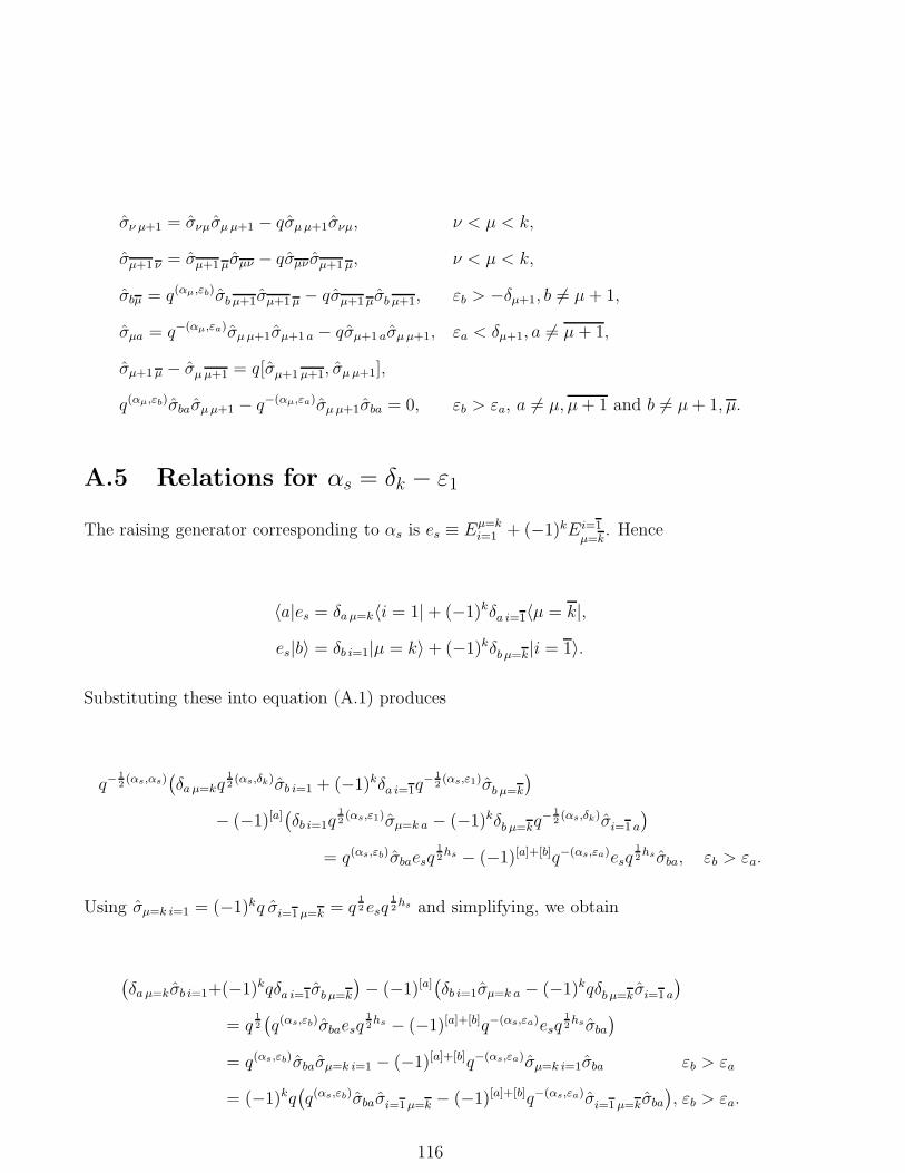
σν µ+1 = σνµσµ µ+1 − qσµ µ+1σνµ, ν < µ < k,

σµ+1 ν = σµ+1 µσµν − qσµν σµ+1 µ, ν < µ < k,

σbµ = q(αµ,εb)σb µ+1σµ+1 µ − qσµ+1 µσb µ+1, εb > −δµ+1, b 6= µ+ 1,

σµa = q−(αµ,εa)σµ µ+1σµ+1 a − qσµ+1 aσµ µ+1, εa < δµ+1, a 6= µ+ 1,

σµ+1 µ − σµ µ+1 = q[σµ+1 µ+1, σµ µ+1],

q(αµ,εb)σbaσµ µ+1 − q−(αµ,εa)σµ µ+1σba = 0, εb > εa, a 6= µ, µ+ 1 and b 6= µ+ 1, µ.

A.5 Relations for αs = δk − ε1

The raising generator corresponding to αs is es ≡ Eµ=ki=1 + (−1)kEi=1

µ=k. Hence

〈a|es = δa µ=k〈i = 1| + (−1)kδa i=1〈µ = k|,

es|b〉 = δb i=1|µ = k〉 + (−1)kδb µ=k|i = 1〉.

Substituting these into equation (A.1) produces

q−12(αs,αs)

(

δa µ=kq12(αs,δk)σb i=1 + (−1)kδa i=1q

− 12(αs,ε1)σb µ=k

)

− (−1)[a](

δb i=1q12(αs,ε1)σµ=k a − (−1)kδb µ=kq

− 12(αs,δk)σi=1 a

)

= q(αs,εb)σbaesq12hs − (−1)[a]+[b]q−(αs,εa)esq

12hsσba, εb > εa.

Using σµ=k i=1 = (−1)kq σi=1 µ=k = q12esq

12hs and simplifying, we obtain

(

δa µ=kσb i=1+(−1)kqδa i=1σb µ=k

)

− (−1)[a](

δb i=1σµ=k a − (−1)kqδb µ=kσi=1 a

)

= q12

(

q(αs,εb)σbaesq12hs − (−1)[a]+[b]q−(αs,εa)esq

12hsσba

)

= q(αs,εb)σbaσµ=k i=1 − (−1)[a]+[b]q−(αs,εa)σµ=k i=1σba εb > εa

= (−1)kq(

q(αs,εb)σbaσi=1 µ=k − (−1)[a]+[b]q−(αs,εa)σi=1 µ=kσba

)

, εb > εa.

116

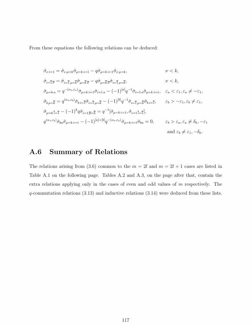
From these equations the following relations can be deduced:

σν i=1 = σν µ=kσµ=k i=1 − qσµ=k i=1σν µ=k, ν < k,

σi=1 ν = σi=1 µ=kσµ=k ν − qσµ=k ν σi=1 µ=k, ν < k,

σµ=k a = q−(αs,εa)σµ=k i=1σi=1 a − (−1)[a]q−1σi=1 aσµ=k i=1, εa < ε1, εa 6= −ε1,

σb µ=k = q(αs,εb)σb i=1σi=1 µ=k − (−1)[b]q−1σi=1 µ=kσb i=1, εb > −ε1, εb 6= ε1,

σµ=k i=1 − (−1)kqσi=1 µ=k = q−1[σµ=k i=1, σi=1 i=1],

q(αs,εb)σbaσµ=k i=1 − (−1)[a]+[b]q−(αs,εa)σµ=k i=1σba = 0, εb > εa, εa 6= δk,−ε1

and εb 6= ε1,−δk.

A.6 Summary of Relations

The relations arising from (3.6) common to the m = 2l and m = 2l + 1 cases are listed in

Table A.1 on the following page. Tables A.2 and A.3, on the page after that, contain the

extra relations applying only in the cases of even and odd values of m respectively. The

q-commutation relations (3.13) and inductive relations (3.14) were deduced from these lists.

117

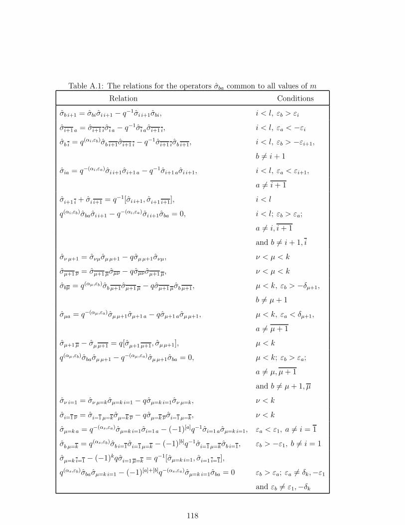
Table A.1: The relations for the operators σba common to all values of m

Relation Conditions

σb i+1 = σbiσi i+1 − q−1σi i+1σbi, i < l, εb > εi

σi+1 a = σi+1 iσi a − q−1σi aσi+1 i, i < l, εa < −εi

σb i = q(αi,εb)σb i+1σi+1 i − q−1σi+1 iσb i+1, i < l, εb > −εi+1,

b 6= i+ 1

σia = q−(αi,εa)σi i+1σi+1 a − q−1σi+1 aσi i+1, i < l, εa < εi+1,

a 6= i+ 1

σi+1 i + σi i+1 = q−1[σi i+1, σi+1 i+1], i < l

q(αi,εb)σbaσi i+1 − q−(αi,εa)σi i+1σba = 0, i < l; εb > εa;

a 6= i, i+ 1

and b 6= i+ 1, i

σν µ+1 = σνµσµ µ+1 − qσµ µ+1σνµ, ν < µ < k

σµ+1 ν = σµ+1 µσµν − qσµν σµ+1 µ, ν < µ < k

σbµ = q(αµ,εb)σb µ+1σµ+1 µ − qσµ+1 µσb µ+1, µ < k, εb > −δµ+1,

b 6= µ+ 1

σµa = q−(αµ,εa)σµ µ+1σµ+1 a − qσµ+1 aσµ µ+1, µ < k, εa < δµ+1,

a 6= µ+ 1

σµ+1 µ − σµ µ+1 = q[σµ+1 µ+1, σµ µ+1], µ < k

q(αµ,εb)σbaσµ µ+1 − q−(αµ,εa)σµ µ+1σba = 0, µ < k; εb > εa;

a 6= µ, µ+ 1

and b 6= µ+ 1, µ

σν i=1 = σν µ=kσµ=k i=1 − qσµ=k i=1σν µ=k, ν < k

σi=1 ν = σi=1 µ=kσµ=k ν − qσµ=k ν σi=1 µ=k, ν < k

σµ=k a = q−(αs,εa)σµ=k i=1σi=1 a − (−1)[a]q−1σi=1 aσµ=k i=1, εa < ε1, a 6= i = 1

σb µ=k = q(αs,εb)σb i=1σi=1 µ=k − (−1)[b]q−1σi=1 µ=kσb i=1, εb > −ε1, b 6= i = 1

σµ=k i=1 − (−1)kqσi=1 µ=k = q−1[σµ=k i=1, σi=1 i=1],

q(αs,εb)σbaσµ=k i=1 − (−1)[a]+[b]q−(αs,εa)σµ=k i=1σba = 0 εb > εa; εa 6= δk,−ε1

and εb 6= ε1,−δk

118

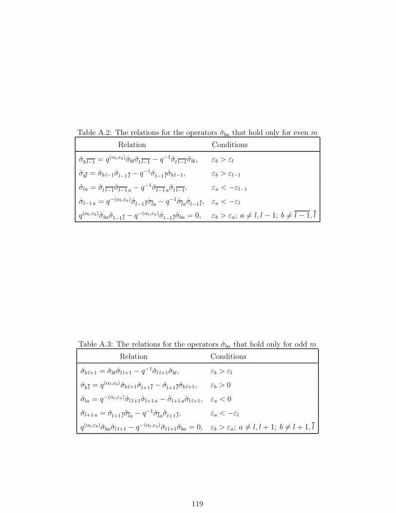
Table A.2: The relations for the operators σba that hold only for even m

Relation Conditions

σb l−1 = q(αl,εb)σblσl l−1 − q−1σl l−1σbl, εb > εl

σbl = σb l−1σl−1 l − q−1σl−1 lσb l−1, εb > εl−1

σla = σl l−1σl−1 a − q−1σl−1 aσl l−1, εa < −εl−1

σl−1 a = q−(αl,εa)σl−1 lσla − q−1σlaσl−1 l, εa < −εl

q(αl,εb)σbaσl−1 l − q−(αl,εa)σl−1 lσba = 0, εb > εa; a 6= l, l − 1; b 6= l − 1, l

Table A.3: The relations for the operators σba that hold only for odd m

Relation Conditions

σb l+1 = σblσl l+1 − q−1σl l+1σbl, εb > εl

σb l = q(αl,εb)σb l+1σl+1 l − σl+1 lσb l+1, εb > 0

σla = q−(αl,εa)σl l+1σl+1 a − σl+1 aσl l+1, εa < 0

σl+1 a = σl+1 lσla − q−1σlaσl+1 l, εa < −εl

q(αl,εb)σbaσl l+1 − q−(αl,εa)σl l+1σba = 0, εb > εa; a 6= l, l + 1; b 6= l + 1, l

119

solutions to the yang-baxter equation and casimir … have already been answered for the aand...

Documents