solow model - macroeconomics ii (econ-6395) · pdf filesolow model omer ozak smu macroeconomic...
TRANSCRIPT
Solow Model
Omer Ozak
SMU
Macroeconomic Theory II
Omer Ozak (SMU) Economic Growth Macroeconomic Theory II 1 / 142
Solow Growth Model
Section 1
Solow Growth Model
Omer Ozak (SMU) Economic Growth Macroeconomic Theory II 2 / 142
Solow Growth Model Solow Growth Model
Solow Growth Model
Develop a simple framework for the proximate causes and themechanics of economic growth and cross-country income differences.
Solow-Swan model named after Robert (Bob) Solow and TrevorSwan, or simply the Solow model
Before Solow growth model, the most common approach to economicgrowth built on the Harrod-Domar model.
Harrod-Domar model emphasized potential dysfunctional aspects ofgrowth: e.g, how growth could go hand-in-hand with increasingunemployment.
At the center of the Solow growth model is the neoclassical aggregateproduction function.
Omer Ozak (SMU) Economic Growth Macroeconomic Theory II 3 / 142
Solow Growth Model The Economic Environment of the Basic Solow Model
The Economic Environment of the Basic Solow Model
Study of economic growth and development necessitates dynamicmodels.
Despite its simplicity, the Solow growth model is a dynamic generalequilibrium model (though many key features of dynamic generalequilibrium models, such as preferences and dynamic optimization aremissing in this model).
Solow is an algebraic or graphical solution to growth
One Sector, one good, no government, closed economy no foreignsector
One representative consumer / household saves s ∈ (0, 1) of income,consumes (1− s), performs 1 unit of labor (L(t)).
One representative firm, uses K , L in production.
Omer Ozak (SMU) Economic Growth Macroeconomic Theory II 4 / 142

Solow Growth Model Households and Production
Households and Production I
Closed economy, with a unique final good. No foreign sector. Onegood = one sector.
Time running to an infinite horizon, time is indexed by tεT ⊆ R+.
Economy is inhabited by a large number of households, and for nowhouseholds will not be optimizing.
This is the main difference between the Solow model and theneoclassical growth model.
To fix ideas, assume all households are identical, so the economyadmits a representative household. One representative household.One representative consumer.
No government.
Omer Ozak (SMU) Economic Growth Macroeconomic Theory II 5 / 142

Solow Growth Model Households and Production
Households and Production II
Assume households save a constant exogenous fraction s of theirdisposable income
Same assumption used in basic Keynesian models and in theHarrod-Domar model; at odds with reality.
Assume all firms have access to the same production function:economy admits a representative firm, with a representative (oraggregate) production function. One representative firm.
Omer Ozak (SMU) Economic Growth Macroeconomic Theory II 6 / 142

Solow Growth Model Households and Production
Households and Production III
Aggregate production function [P/N F/N] for the unique final good is
Y (t) = F [K (t) , L (t) ,A (t)] (1)
Assume capital is the same as the final good of the economy, butused in the production process of more goods.
A (t) is a shifter of the P/N F/N (1). Broad notion of technology.
Major assumption: technology is free; it is publicly available as anon-excludable, non-rival good.
Omer Ozak (SMU) Economic Growth Macroeconomic Theory II 7 / 142

Solow Growth Model Households and Production
First Key Assumption
Assumption 1 (Continuity, Twice Continuously Differentiability,Positive and Diminishing Marginal Products, andConstant Returns to Scale) The production functionF : R3
+ → R+ is twice continuously differentiable in K andL, and satisfies
FK (K , L,A) ≡ ∂F (·)∂K
> 0, FL(K , L,A) ≡ ∂F (·)∂L
> 0,
FKK (K , L,A) ≡ ∂2F (·)∂K 2
< 0, FLL(K , L,A) ≡ ∂2F (·)∂L2
< 0.
Omer Ozak (SMU) Economic Growth Macroeconomic Theory II 8 / 142

Solow Growth Model Households and Production
First Key Assumption
Moreover, F exhibits constant returns to scale [CRS] in K and L.
Assume F exhibits constant returns to scale in K and L:F (λK , λL,A) = λF (K , L,A) ∀ λ ∈ R+. I.e., it is linearlyhomogeneous (homogeneous of degree 1) in these two variables.
Omer Ozak (SMU) Economic Growth Macroeconomic Theory II 9 / 142
Solow Growth Model Households and Production
Review
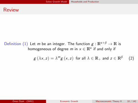
Definition (1) Let m be an integer. The function g : Rα+β → R ishomogeneous of degree m in x ∈ Rα if and only if
g (λx , z) = λmg (x , z) for all λ ∈ R+ and z ∈ Rβ (2)
Omer Ozak (SMU) Economic Growth Macroeconomic Theory II 10 / 142

Solow Growth Model Households and Production
Review
Theorem (Euler’s Theorem) (∀α ∈N, shown for α = 2) Supposethat g : Rα+β → R is continuously differentiable in x1 ∈ R
and x2 ∈ R, with partial derivatives denoted by gx1 and gx2
and is homogeneous of degree m in x1 and x2. Then
mg (x1, x2, z) = ∇xg(·) · x = gx1 (x , z) x1 + gx2 (x , z) x2
for all x ∈ Rα and z ∈ Rβ.
Moreover, gx1 (x1, x2, z) and gx2 (x1, x2, z) are themselveshomogeneous of degree m− 1 in x1 and x2.
Omer Ozak (SMU) Economic Growth Macroeconomic Theory II 11 / 142

Solow Growth Model Households and Production
Second Key Assumption
Assumption 2 (Inada conditions) F satisfies the Inada conditions
limK→0
FK (·) = ∞, and limK→∞
FK (·) = 0 ∀ A, L > 0,
limL→0
FL (·) = ∞, and limL→∞
FL (·) = 0 ∀ A, K > 0.
Works nicely with intermediate value theorem:∀ γ ∈ R+ , ∃ a unique k such that [s.t.] Fk (·) = γ
This can be observed graphically as FK (0, ·) = ∞, & FK (∞, ·) = 0
Important in ensuring the existence of interior equilibria.
It can be relaxed quite a bit, though useful to get us started.
Omer Ozak (SMU) Economic Growth Macroeconomic Theory II 12 / 142

Solow Growth Model Households and Production
Second Key Assumption
We assume that inputs and outputs are exchanged in competitivemarkets.
A production function is Neoclassical if it satisfies Assumptions 1and 2.
Note Assumptions 1 and 2: → F (K , 0,A) = F (0, L,A) = 0 ∀K , L,A
Omer Ozak (SMU) Economic Growth Macroeconomic Theory II 13 / 142
Solow Growth Model Households and Production
Production Functions34 . Chapter 2 The Solow Growth Model
0K
A
F(K, L, A) F(K, L, A)
0K
B
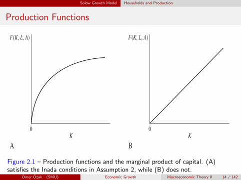
FIGURE 2.1 Production functions. (A) satisfies the Inada conditions in Assumption 2, while (B)does not.
are highly productive and that when capital or labor are sufficiently abundant, their marginalproducts are close to zero. The condition that F(0, L, A) = 0 for all L and A makes capital anessential input. This aspect of the assumption can be relaxed without any major implicationsfor the results in this book. Figure 2.1 shows the production function F(K, L, A) as a functionof K , for given L and A, in two different cases; in panel A the Inada conditions are satisfied,while in panel B they are not.
I refer to Assumptions 1 and 2, which can be thought of as the neoclassical technologyassumptions, throughout much of the book. For this reason, they are numbered independentlyfrom the equations, theorems, and proposition in this chapter.
2.2 The Solow Model in Discrete Time
I next present the dynamics of economic growth in the discrete-time Solow model.
2.2.1 Fundamental Law of Motion of the Solow Model
Recall that K depreciates exponentially at the rate δ, so that the law of motion of the capitalstock is given by
K(t + 1) = (1 − δ) K(t) + I (t), (2.8)
where I (t) is investment at time t .From national income accounting for a closed economy, the total amount of final good in
the economy must be either consumed or invested, thus
Y (t) = C(t) + I (t), (2.9)
where C(t) is consumption.2 Using (2.1), (2.8), and (2.9), any feasible dynamic allocation inthis economy must satisfy
K(t + 1) ≤ F(K(t), L(t), A(t)) + (1 − δ)K(t) − C(t)
2. In addition, we can introduce government spending G(t) on the right-hand side of (2.9). Government spendingdoes not play a major role in the Solow growth model, thus its introduction is relegated to Exercise 2.7.
Figure 2.1 – Production functions and the marginal product of capital. (A)satisfies the Inada conditions in Assumption 2, while (B) does not.
Omer Ozak (SMU) Economic Growth Macroeconomic Theory II 14 / 142

Solow Growth Model Market Structure, Endowments and Market Clearing
Market Structure, Endowments and Market Clearing I
We will assume that markets are competitive, so ours will be aprototypical competitive general equilibrium model.
Households own all of the labor, which they supply inelastically.
Endowment of labor in the economy, L (t), and all of this will besupplied regardless of the price.
The labor market clearing condition can then be expressed as:
L (t) = L (t) (3)
∀ t, where L (t) denotes the demand for labor (and also the level ofemployment). And L (t) denotes labor supply.
Omer Ozak (SMU) Economic Growth Macroeconomic Theory II 15 / 142

Solow Growth Model Market Structure, Endowments and Market Clearing
Market Structure, Endowments and Market Clearing II
More generally, should be written in complementary slackness form.
In particular, let the wage rate at time t be w (t), then the labormarket clearing condition takes the form:
L (t) ≤ L (t) , w (t) ≥ 0, and [L (t)− L (t)]w (t) = 0 (4)
But Assumption 1 and competitive labor markets make sure thatwages have to be strictly positive.
Omer Ozak (SMU) Economic Growth Macroeconomic Theory II 16 / 142
Solow Growth Model Market Structure, Endowments and Market Clearing
Market Structure, Endowments and Market Clearing III
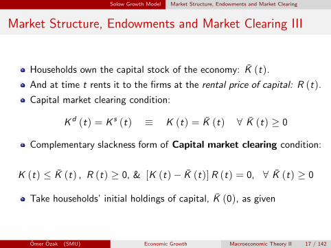
Households own the capital stock of the economy: K (t).
And at time t rents it to the firms at the rental price of capital: R (t).
Capital market clearing condition:
Kd (t) = K s (t) ≡ K (t) = K (t) ∀ K (t) ≥ 0
Complementary slackness form of Capital market clearing condition:
K (t) ≤ K (t) , R (t) ≥ 0, & [K (t)− K (t)]R (t) = 0, ∀ K (t) ≥ 0
Take households’ initial holdings of capital, K (0), as given
Omer Ozak (SMU) Economic Growth Macroeconomic Theory II 17 / 142

The Solow Model in Discrete Time
Section 2
The Solow Model in Discrete Time
Omer Ozak (SMU) Economic Growth Macroeconomic Theory II 18 / 142
The Solow Model in Discrete Time
Solow Model in Discrete Time
Our notation until now is such that t could be discrete or continuous(careful book makes no distinction whatsoever)
So x(t) could be the path of variable x in either case...but payattention some equations change when using continuous instead ofdiscrete time.
Here we will use xt for discrete time and x(t) for continuous (do thesame in your notes, exams, etc.)
Omer Ozak (SMU) Economic Growth Macroeconomic Theory II 19 / 142
The Solow Model in Discrete Time
Relating prices and interest rates
Pt is the price of the final good at time t, normalize the price of thefinal good to 1 in all periods.
Building on an insight by Kenneth Arrow (Arrow, 1964) that it issufficient to price securities (assets) that transfer one unit ofconsumption from one date (or state of the world) to another.
In Arrow-Debreu [A-D] economy prices Pt are linked to Pt+1 by thereal rate of interest from t to t + 1 of rt+1:
Pt/Pt+1 = 1 + rt+1
If Pt = 1, then rt is intertemporal exchange rate; “real” or“commodity” rate of interest ≡ interest rate implied by prices.
rt will enable us to normalize the price to 1 in every period.
Omer Ozak (SMU) Economic Growth Macroeconomic Theory II 20 / 142

The Solow Model in Discrete Time
Market Structure, Endowments and Market Clearing V
A-D General equilibrium economies:
The same good at different dates is a different commodity.
Therefore, there will be an infinite number of commodities.
Assume capital, K , depreciates by constant rate, “exponential form,”at δ ∈ (0, 1): of 1 unit of capital at t, only 1− δ is left at t + 1.
δ affects household rt (rate of return for savings); indifferencebetween lending and investing implies: 1 + rt = Rt + (1− δ).
Interest rate faced by the household will be rt = Rt − δ.
Omer Ozak (SMU) Economic Growth Macroeconomic Theory II 21 / 142

The Solow Model in Discrete Time Firm Optimization
Firm Optimization I
Consider the problem of profit maximization at a representative firm:
πt ≡ maxLt≥0,Kt≥0
F [Kt , Lt ,At ]− wtLt − RtKt . (5)
Since there are no irreversible investments or costs of adjustments, theproduction side can be represented as a static maximization problem.
Equivalently, cost minimization problem.
Omer Ozak (SMU) Economic Growth Macroeconomic Theory II 22 / 142
The Solow Model in Discrete Time Firm Optimization
Firm Optimization II
Features worth noting:
1 Problem is set up in terms of aggregate variables.2 Nothing multiplying the F term, price of the final good has normalized
to 1.3 Already imposes competitive factor markets: firm is taking as given wt
and Rt .4 Concave problem, since F is concave.
Since F (·) satisfies CRS, then either π = 0 or the solution does notexist.
Omer Ozak (SMU) Economic Growth Macroeconomic Theory II 23 / 142
The Solow Model in Discrete Time Firm Optimization
Firm Optimization III
In particular, given wt , Rt and At the Firms demand for Lt and Kt isgiven by the solution to the FOC.
Since F is differentiable, first-order necessary conditions imply:
wt = FL[K t , Lt ,At ] > 0, (6)
andRt = FK [K t , Lt ,At ] > 0. (7)
Note also that in (6) and (7), we used Kt and Lt , the amount ofcapital and labor used by firms.
In fact, solving for Kt and Lt , we can derive the capital and labordemands of firms in this economy at rental prices Rt and wt .
Thus we could have used Kdt instead of Kt , but this additional
notation is not necessary.
Omer Ozak (SMU) Economic Growth Macroeconomic Theory II 24 / 142
The Solow Model in Discrete Time Firm Optimization
Firm Optimization IV
Alternative solution uses Assumption 1, F (·) is homogeneous ofdegree 1 in Lt and Kt , and Euler’s Theorem with m = 1 is CRS:
Yt = F [Kt , Lt ,At ]
= FL [Kt , Lt ,At ] · Lt + FK [Kt , Lt ,At ] ·Kt
πt = FL (·) · Lt + FK (·) ·Kt − wtLt − RtKt
= {FL (·)− wt} · Lt + {FK (·)− Rt} ·Kt
Where in equilibrium must have πt = 0, which will only hold if both(6) and (7) hold, and L∗ = Lt = Lt and K ∗ = Kt = Kt .
Omer Ozak (SMU) Economic Growth Macroeconomic Theory II 25 / 142
The Solow Model in Discrete Time Firm Optimization
Firm Optimization V
Proposition (1) Suppose Assumption 1 holds. Then in an equilibrium of aSolow growth model, firms make no profits, and in particular,
Yt = wtLt + RtKt .
Proof: As above Euler Thm; substitute (6) and (7) above into Yt .
Thus πt = 0, so we do not need to specify firm ownership.
Omer Ozak (SMU) Economic Growth Macroeconomic Theory II 26 / 142
The Solow Model in Discrete Time Fundamental Law of Motion of the Solow Model
Fundamental Law of Motion of the Solow Model I
Recall that K depreciates exponentially at the rate δ, so
Kt+1 = (1− δ)Kt + It ⇔ 4Kt+1 = It − δKt , (8)
where It is investment at time t.
From national income accounting for a closed economy,
Yt = Ct + It , (9)
Using (1), (8) and (9), any feasible dynamic allocation in thiseconomy must satisfy
Kt+1 ≤ F [Kt , Lt ,At ] + (1− δ)Kt − Ct ∀t ∈N or Z+
Omer Ozak (SMU) Economic Growth Macroeconomic Theory II 27 / 142
The Solow Model in Discrete Time Fundamental Law of Motion of the Solow Model
Fundamental Law of Motion of the Solow Model II
Solow model is a mixture of an old-style Keynesian model and amodern dynamic macroeconomic model.
Households do not optimize, but firms still maximize and factormarkets clear.
Note this is not derived from the maximization of utility function:welfare comparisons have to be taken with a grain of salt.
Behavioral rule of the constant saving rate simplifies the structure ofequilibrium considerably.
Omer Ozak (SMU) Economic Growth Macroeconomic Theory II 28 / 142

The Solow Model in Discrete Time Fundamental Law of Motion of the Solow Model
Fundamental Law of Motion of the Solow Model III
Since the economy is closed (and there is no government spending),
St = It = Yt − Ct .
Individuals are assumed to save a constant fraction s of their income,
St = sYt , (10)
Ct = (1− s)Yt (11)
Implies that the supply of capital resulting from households’ behaviorcan be expressed as
K st = (1− δ)Kt + St = (1− δ)Kt + sYt .
Omer Ozak (SMU) Economic Growth Macroeconomic Theory II 29 / 142

The Solow Model in Discrete Time Fundamental Law of Motion of the Solow Model
Fundamental Law of Motion of the Solow Model IV
Setting supply and demand equal to each other, this implies K st = Kt .
From (3), we have Lt = Lt .
Combining these market clearing conditions with (1) and (8), weobtain the fundamental law of motion the Solow growth model:
Kt+1 = sF [Kt , Lt ,At ] + (1− δ)Kt . (12)
Nonlinear difference equation.
Equilibrium of the Solow growth model is described by this equationtogether with laws of motion for Lt (or Lt) and At .
Omer Ozak (SMU) Economic Growth Macroeconomic Theory II 30 / 142
The Solow Model in Discrete Time Definition of Equilibrium
Definition of Equilibrium I
Definition (2) In the basic Solow model for a given sequence of{Lt ,At}∞
t=0 and an initial capital stock K0, an equilibriumpath is a sequence of capital stocks, output levels,consumption levels, wages and rental rates {Kt ,Yt ,Ct ,wt ,Rt}∞
t=0 such that Kt satisfies (12), Yt is given by (1), wt andRt are given by (6) and (7), and Ct is given by (11).
Kt+1 = sF [Kt , Lt ,At ] + (1− δ)Kt , Yt = F [Kt , Lt ,At ] ,wt = FL [Kt , Lt ,At ] > 0 , Rt = FK [Kt , Lt ,At ] > 0 ,Ct = (1− s)Yt , It = St = sYt , rt = Rt − δ
Note an equilibrium is defined as an entire path of allocations andprices: not a static object.
Omer Ozak (SMU) Economic Growth Macroeconomic Theory II 31 / 142
The Solow Model in Discrete Time Equilibrium
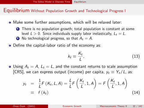
Equilibrium Without Population Growth and Technological Progress I
Make some further assumptions, which will be relaxed later:
1 There is no population growth; total population is constant at somelevel L > 0. Since individuals supply labor inelastically, Lt = L.
2 No technological progress, so that At = A.
Define the capital-labor ratio of the economy as:
kt ≡Kt
L, (13)
Using At = A, Lt = L, and the constant returns to scale assumption[CRS], we can express output (income) per capita, yt ≡ Yt/L, as:
yt =1
LF (Kt , L,A) =
L
LF
(Kt
L, 1,A
)= F
(Kt
L, 1,A
)≡ f (kt) (14)
Omer Ozak (SMU) Economic Growth Macroeconomic Theory II 32 / 142

The Solow Model in Discrete Time Equilibrium
Equilibrium Without Population Growth nor Technological Progress II
ct =Ct
L= (1− s)
Yt
L= (1− s) yt
Note that f (kt) here depends on A, so we could write f (kt ,A); butA is constant and can be normalized to A = 1.
From the Euler Theorem,
Rt = FK (K , L,A) = FK
(K
L, 1,A
)= f ′ (kt) > 0 and
wt = FL (K , L,A) = f (kt)− kt f′ (kt) > 0. (15)
Both are positive from Assumption 1.
Omer Ozak (SMU) Economic Growth Macroeconomic Theory II 33 / 142

The Solow Model in Discrete Time Equilibrium
Example:The Cobb-Douglas Production Function I
Cobb-Douglas is a very special production function and manyinteresting phenomena are ruled out, but it is widely used:
Yt = F [Kt , Lt ,At ]
= AK αt L
1−αt , 0 < α < 1. (16)
Satisfies Assumptions 1 and 2.Dividing both sides by Lt ,
yt = f (kt , 1,A) = Akαt ,
From equation (15),
Rt =∂Akα
t
∂kt= αAk
−(1−α)t .
From the Euler Theorem,
wt = yt − Rtkt = (1− α)Akαt .
Omer Ozak (SMU) Economic Growth Macroeconomic Theory II 34 / 142
The Solow Model in Discrete Time Equilibrium
Example:The Cobb-Douglas Production Function II
Alternatively, in terms of the original Cobb-Douglas productionfunction (16),
Rt = αAK α−1t L1−α
t
= αAk−(1−α)t ,
Similarly, from (15),
wt = Akαt − kt · αAk−(1−α)
t
= (1− α)AK αt L−αt ,
= (1− α)Akαt ,
Which verifies the alternative expression for the wage rate in (6)
Omer Ozak (SMU) Economic Growth Macroeconomic Theory II 35 / 142

The Solow Model in Discrete Time Equilibrium
Equilibrium Without Population Growth and Technological Progress III
The per capita representation of the aggregate production functionenables us to divide both sides of (12) by L to obtain:
kt+1 = sf (kt) + (1− δ) kt . (17)
Since it is derived from (12), it also can be referred to as theequilibrium difference equation of the Solow model
The other equilibrium quantities can be obtained from thecapital-labor ratio kt .
Definition (3) A steady-state equilibrium without technological progressand population growth is an equilibrium path in whichkt = k∗ for all t.
The economy will tend to this steady state equilibrium over time (butnever reach it in finite time).
Omer Ozak (SMU) Economic Growth Macroeconomic Theory II 36 / 142
The Solow Model in Discrete Time Equilibrium
Steady-State Capital-Labor Ratio38 . Chapter 2 The Solow Growth Model
0 k*
k(t)
k(t � 1)
sf (k(t)) � (1 � •)k(t)k*
45°
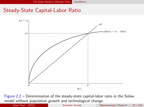
FIGURE 2.2 Determination of the steady-state capital-labor ratio in the Solow model without populationgrowth and technological change.
represents the right-hand side of (2.17) and the dashed line corresponds to the 45◦ line. Their(positive) intersection gives the steady-state value of the capital-labor ratio k∗, which satisfies
f (k∗)k∗ = δ
s. (2.18)
Notice that in Figure 2.2 there is another intersection between (2.17) and the 45◦
line at k = 0.This second intersection occurs because, from Assumption 2, capital is an essential input, andthus f (0) = 0. Starting with k(0) = 0, there will then be no savings, and the economy willremain at k = 0. Nevertheless, I ignore this intersection throughout for a number of reasons.First, k = 0 is a steady-state equilibrium only when capital is an essential input and f (0) = 0.But as noted above, this assumption can be relaxed without any implications for the rest of theanalysis, and when f (0) > 0, k = 0 is no longer a steady-state equilibrium. This is illustratedin Figure 2.3, which draws (2.17) for the case where f (0) = ε for some ε > 0. Second, as wewill see below, this intersection, even when it exists, is an unstable point; thus the economywould never travel toward this point starting with K(0) > 0 (or with k(0) > 0). Finally, andmost importantly, this intersection holds no economic interest for us.4
An alternative visual representation shows the steady state as the intersection between aray through the origin with slope δ (representing the function δk) and the function sf (k).Figure 2.4, which illustrates this representation, is also useful for two other purposes. First,it depicts the levels of consumption and investment in a single figure. The vertical distancebetween the horizontal axis and the δk line at the steady-state equilibrium gives the amount of
4. Hakenes and Irmen (2006) show that even with f (0) = 0, the Inada conditions imply that in the continuous-time version of the Solow model k = 0 may not be the only equilibrium and the economy may move awayfrom k = 0.
Figure 2.2 – Determination of the steady-state capital-labor ratio in the Solowmodel without population growth and technological change.
Omer Ozak (SMU) Economic Growth Macroeconomic Theory II 37 / 142
The Solow Model in Discrete Time Equilibrium
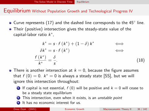
Equilibrium Without Population Growth and Technological Progress IV
Curve represents (17) and the dashed line corresponds to the 45◦ line.
Their (positive) intersection gives the steady-state value of thecapital-labor ratio k∗,
k∗ = s · f (k∗) + (1− δ) k∗ ⇐⇒δk∗ = s · f (k∗) ⇐⇒
f (k∗)
k∗=
δ
s. (18)
There is another intersection at k = 0, because the figure assumesthat f (0) = 0. k∗ = 0 is always a steady state [SS], but we willignore this intersection throughout:
1 If capital is not essential, f (0) will be positive and k = 0 will cease tobe a steady state equilibrium
2 This intersection, even when it exists, is an unstable point3 It has no economic interest for us.
Omer Ozak (SMU) Economic Growth Macroeconomic Theory II 38 / 142
The Solow Model in Discrete Time Equilibrium
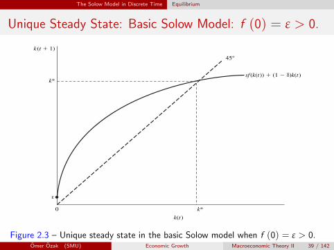
Unique Steady State: Basic Solow Model: f (0) = ε > 0.2.2 The Solow Model in Discrete Time . 39
©
0 k*
k(t)
k(t � 1)
sf (k(t)) � (1 � •)k(t)k*
45°
FIGURE 2.3 Unique steady state in the basic Solow model when f (0) = ε > 0.
investment per capita at the steady-state equilibrium (equal to δk∗), while the vertical distancebetween the function f (k) and the δk line at k∗ gives the level of consumption per capita.Clearly, the sum of these two terms make up f (k∗). Second, Figure 2.4 also emphasizes thatthe steady-state equilibrium in the Solow model essentially sets investment, sf (k), equal tothe amount of capital that needs to be replenished, δk. This interpretation is particularly usefulwhen population growth and technological change are incorporated.
This analysis therefore leads to the following proposition (with the convention that theintersection at k = 0 is being ignored even though f (0) = 0).
Proposition 2.2 Consider the basic Solow growth model and suppose that Assumptions 1and 2 hold. Then there exists a unique steady-state equilibrium where the capital-labor ratiok∗ ∈ (0, ∞) satisfies (2.18), per capita output is given by
y∗ = f (k∗), (2.19)
and per capita consumption is given by
c∗ = (1 − s) f (k∗). (2.20)
Proof. The preceding argument establishes that any k∗ that satisfies (2.18) is a steady state.To establish existence, note that from Assumption 2 (and from l’Hopital’s Rule, see TheoremA.21 in Appendix A), limk→0 f (k)/k = ∞ and limk→∞ f (k)/k = 0. Moreover, f (k)/k iscontinuous from Assumption 1, so by the Intermediate Value Theorem (Theorem A.3) thereexists k∗ such that (2.18) is satisfied. To see uniqueness, differentiate f (k)/k with respect tok, which gives
∂(f (k)/k)
∂k= f ′(k)k − f (k)
k2= − w
k2< 0, (2.21)
Figure 2.3 – Unique steady state in the basic Solow model when f (0) = ε > 0.Omer Ozak (SMU) Economic Growth Macroeconomic Theory II 39 / 142
The Solow Model in Discrete Time Equilibrium
Equilibrium Without Population Growth and Technological Progress V
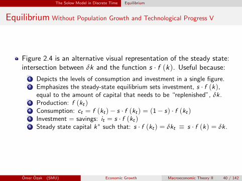
Figure 2.4 is an alternative visual representation of the steady state:intersection between δk and the function s · f (k). Useful because:
1 Depicts the levels of consumption and investment in a single figure.2 Emphasizes the steady-state equilibrium sets investment, s · f (k),
equal to the amount of capital that needs to be “replenished”, δk.3 Production: f (kt)4 Consumption: ct = f (kt)− s · f (kt) = (1− s) · f (kt)5 Investment = savings: it = s · f (kt)6 Steady state capital k∗ such that: s · f (kt) = δkt ≡ s · f (k) = δk.
Omer Ozak (SMU) Economic Growth Macroeconomic Theory II 40 / 142

The Solow Model in Discrete Time Equilibrium
Consumption and Investment in Steady StateIntroduction to Modern Economic Growth
output
k(t)
f(k*)
k*
δk(t)
f(k(t))
sf(k*)sf(k(t))
consumption
investment
0
Figure 2.4. Investment and consumption in the steady-state equilibrium.
the capital-labor ratio k∗ ∈ (0,∞) is given by (2.17), per capita output is given by
(2.18) y∗ = f (k∗)
and per capita consumption is given by
(2.19) c∗ = (1− s) f (k∗) .
Proof. The preceding argument establishes that (2.17) any k∗ that satisfies
(2.16) is a steady state. To establish existence, note that from Assumption 2 (and
from L’Hopital’s rule), limk→0 f (k) /k = ∞ and limk→∞ f (k) /k = 0. Moreover,
f (k) /k is continuous from Assumption 1, so by the intermediate value theorem
(see Mathematical Appendix) there exists k∗ such that (2.17) is satisfied. To see
uniqueness, differentiate f (k) /k with respect to k, which gives
(2.20)∂ [f (k) /k]
∂k=
f 0 (k) k − f (k)
k2= −w
k2< 0,
where the last equality uses (2.14). Since f (k) /k is everywhere (strictly) decreasing,
there can only exist a unique value k∗ that satisfies (2.17).
56
Figure 2.4 – Investment and consumption in the steady state equilibrium.Omer Ozak (SMU) Economic Growth Macroeconomic Theory II 41 / 142

The Solow Model in Discrete Time Equilibrium
Equilibrium Without Population Growth and Technological Progress V
Figure 2.4b is an alternate visualization, rate of change in capital, γk :
1 Starting from (17): kt+1 = s · f (kt) + (1− δ) kt2 Rate of change of capital: γkt+1
= kt+1+ktkt
= 4ktkt
= s ·f (kt )kt− δ
3 In graph distance of s · f (kt) /kt from δ is rate of change.
Supplemental Graphs
Omer Ozak (SMU) Economic Growth Macroeconomic Theory II 42 / 142

The Solow Model in Discrete Time Equilibrium
Rate of Change in Capital
Figure 2.4B – Distance of s · f (kt) /kt from δ is rate of change of capital.Omer Ozak (SMU) Economic Growth Macroeconomic Theory II 43 / 142
The Solow Model in Discrete Time Equilibrium
Equilibrium Without Population Growth and Technological Progress VI
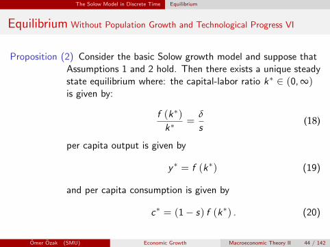
Proposition (2) Consider the basic Solow growth model and suppose thatAssumptions 1 and 2 hold. Then there exists a unique steadystate equilibrium where: the capital-labor ratio k∗ ∈ (0, ∞)is given by:
f (k∗)
k∗=
δ
s(18)
per capita output is given by
y ∗ = f (k∗) (19)
and per capita consumption is given by
c∗ = (1− s) f (k∗) . (20)
Omer Ozak (SMU) Economic Growth Macroeconomic Theory II 44 / 142

The Solow Model in Discrete Time Equilibrium
Proof of Theorem
Existence:
The preceding argument establishes that any k∗ that satisfies (18) isa steady state.
To establish existence, note that by Assumption 2 (and fromL’Hospital’s rule), limk→0 f (k) /k = ∞ and limk→∞ f (k) /k = 0.
Moreover, f (k) /k is continuous by Assumption 1, so by theIntermediate Value Theorem there exists k∗ such that (18) is satisfied.
Omer Ozak (SMU) Economic Growth Macroeconomic Theory II 45 / 142
The Solow Model in Discrete Time Equilibrium
Proof of Theorem
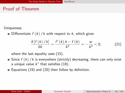
Uniqueness:
Differentiate f (k) /k with respect to k , which gives
∂ [f (k) /k ]∂k
=f ′ (k) k − f (k)
k2= − w
k2< 0, (21)
where the last equality uses (15).
Since f (k) /k is everywhere (strictly) decreasing, there can only exista unique value k∗ that satisfies (18).
Equations (19) and (20) then follow by definition.
Omer Ozak (SMU) Economic Growth Macroeconomic Theory II 46 / 142
The Solow Model in Discrete Time Equilibrium
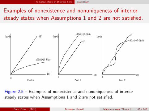
Examples of nonexistence and nonuniqueness of interiorsteady states when Assumptions 1 and 2 are not satisfied.
Introduction to Modern Economic Growth
k(t+1)
k(t)
45°
sf(k(t))+(1–δ)k(t)
0
k(t+1)
k(t)
45°
sf(k(t))+(1–δ)k(t)
0
k(t+1)
k(t)
45°
sf(k(t))+(1–δ)k(t)
0Panel A Panel B Panel C
Figure 2.5. Examples of nonexistence and nonuniqueness of steadystates when Assumptions 1 and 2 are not satisfied.
Equation (2.18) and (2.19) then follow by definition. ¤
Figure 2.5 shows through a series of examples why Assumptions 1 and 2 cannot
be dispensed with for the existence and uniqueness results in Proposition 2.2. In
the first two panels, the failure of Assumption 2 leads to a situation in which there
is no steady state equilibrium with positive activity, while in the third panel, the
failure of Assumption 1 leads to non-uniqueness of steady states.
So far the model is very parsimonious: it does not have many parameters and
abstracts from many features of the real world in order to focus on the question of
interest. Recall that an understanding of how cross-country differences in certain
parameters translate into differences in growth rates or output levels is essential for
our focus. This will be done in the next proposition. But before doing so, let us
generalize the production function in one simple way, and assume that
f (k) = af (k) ,
where a > 0, so that a is a shift parameter, with greater values corresponding to
greater productivity of factors. This type of productivity is referred to as “Hicks-
neutral” as we will see below, but for now it is just a convenient way of looking
at the impact of productivity differences across countries. Since f (k) satisfies the
regularity conditions imposed above, so does f (k).
57
Figure 2.5 – Examples of nonexistence and nonuniqueness of interiorsteady states when Assumptions 1 and 2 are not satisfied.
Omer Ozak (SMU) Economic Growth Macroeconomic Theory II 47 / 142

The Solow Model in Discrete Time Equilibrium
Equilibrium Without Population Growth and Technological Progress VII
Figure shows through a series of examples why Assumptions 1 and 2cannot be dispensed with for the existence and uniqueness results.
(A) and (B): the failure of Assumption 2 leads to a situation in whichthere is no steady state equilibrium with positive activity.
(C): the failure of Assumption 1 leads to non-uniqueness of steadystates.
Omer Ozak (SMU) Economic Growth Macroeconomic Theory II 48 / 142
The Solow Model in Discrete Time Equilibrium
Equilibrium Without Population Growth and Technological Progress VIII
Generalize the production function in one simple way, and assume that
f (k) = Af (k) ,
A > 0, so that a is a (“Hicks-neutral”) shift parameter, with greatervalues corresponding to greater productivity of factors..
Since f (k) satisfies the regularity conditions imposed above, so doesf (k).
Omer Ozak (SMU) Economic Growth Macroeconomic Theory II 49 / 142
The Solow Model in Discrete Time Equilibrium
Equilibrium Without Population Growth and Technological Progress IX
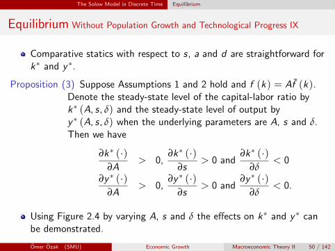
Comparative statics with respect to s, a and d are straightforward fork∗ and y ∗.
Proposition (3) Suppose Assumptions 1 and 2 hold and f (k) = Af (k).Denote the steady-state level of the capital-labor ratio byk∗ (A, s, δ) and the steady-state level of output byy ∗ (A, s, δ) when the underlying parameters are A, s and δ.Then we have
∂k∗ (·)∂A
> 0,∂k∗ (·)
∂s> 0 and
∂k∗ (·)∂δ
< 0
∂y ∗ (·)∂A
> 0,∂y ∗ (·)
∂s> 0 and
∂y ∗ (·)∂δ
< 0.
Using Figure 2.4 by varying A, s and δ the effects on k∗ and y ∗ canbe demonstrated.
Omer Ozak (SMU) Economic Growth Macroeconomic Theory II 50 / 142

The Solow Model in Discrete Time Equilibrium
Varying A, s and δ: effects on k∗ and y ∗
Figure 2.5 – Examples of varying A, s and δ to determine the effects on k∗
and y ∗.
Omer Ozak (SMU) Economic Growth Macroeconomic Theory II 51 / 142

The Solow Model in Discrete Time Equilibrium
Equilibrium Without Population Growth and Technological Progress IX
Proof of comparative static results: follows immediately by writing
f (k∗)
k∗=
δ
As
Now apply the implicit function theorem to obtain the results.
For example,∂k∗
∂s=
δ (k∗)2
s2w ∗> 0
where w ∗ = f (k∗)− k∗f ′ (k∗) > 0.
The other results follow similarly.
Omer Ozak (SMU) Economic Growth Macroeconomic Theory II 52 / 142
The Solow Model in Discrete Time Equilibrium
Equilibrium Without Population Growth and Technological Progress X
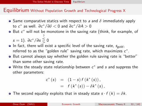
Same comparative statics with respect to a and δ immediately applyto c∗ as well. ∂c∗/∂δ < 0 and ∂c∗/∂A > 0But c∗ will not be monotone in the saving rate (think, for example, of
s = 1). ∂c∗/∂s?
Q 0In fact, there will exist a specific level of the saving rate, sgold ,referred to as the “golden rule” saving rate, which maximizes c∗.But cannot always say whether the golden rule saving rate is “better”than some other saving rate.Write the steady state relationship between c∗ and s and suppress theother parameters:
c∗ (s) = (1− s) f (k∗ (s)) ,
= f (k∗ (s))− δk∗ (s) ,
The second equality exploits that in steady state s · f (k) = δk .
Omer Ozak (SMU) Economic Growth Macroeconomic Theory II 53 / 142

The Solow Model in Discrete Time Equilibrium
Equilibrium Without Population Growth and Technological Progress XI
Differentiating with respect to s,
∂c∗ (s)
∂s=[f ′ (k∗ (s))− δ
] ∂k∗
∂s. (22)
sgold is such that ∂c∗ (sgold ) /∂s = 0 (FOC) (Verify SOC holds). Thecorresponding steady-state golden rule capital stock is defined ask∗gold .
Proposition (4) In the basic Solow growth model, the highest level ofsteady-state consumption is reached for sgold , with thecorresponding steady state capital level k∗gold such that
f ′(k∗gold
)= δ. (23)
Omer Ozak (SMU) Economic Growth Macroeconomic Theory II 54 / 142

The Solow Model in Discrete Time Equilibrium
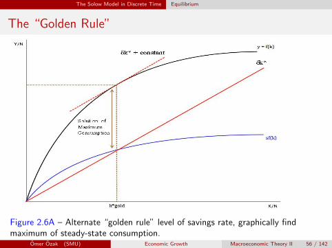
The “Golden Rule”2.3 Transitional Dynamics in the Discrete-Time Solow Model . 43
0 1Saving rate
s*gold
Consumption
gold(l � s)f(k* )
FIGURE 2.6 The golden rule level of saving rate, which maximizes steady-state consumption.
must be considered with caution. In fact, the reason this type of dynamic inefficiency does notgenerally apply when consumption-saving decisions are endogenized may already be apparentto many of you.
2.3 Transitional Dynamics in the Discrete-Time Solow Model
Proposition 2.2 establishes the existence of a unique steady-state equilibrium (with positiveactivity). Recall that an equilibrium path does not refer simply to the steady state but to theentire path of capital stock, output, consumption, and factor prices. This is an important pointto bear in mind, especially since the term “equilibrium” is used differently in economics thanin other disciplines. Typically, in engineering and the physical sciences, an equilibrium refersto a point of rest of a dynamical system, thus to what I have so far referred to as “the steady-state equilibrium.” One may then be tempted to say that the system is in “disequilibrium” whenit is away from the steady state. However, in economics, the non-steady-state behavior of aneconomy is also governed by market clearing and optimizing behavior of households and firms.Most economies spend much of their time in non-steady-state situations. Thus we are typicallyinterested in the entire dynamic equilibrium path of the economy, not just in its steady state.
To determine what the equilibrium path of our simple economy looks like, we need tostudy the transitional dynamics of the equilibrium difference equation (2.17) starting from anarbitrary capital-labor ratio, k(0) > 0. Of special interest are the answers to the questions ofwhether the economy will tend to this steady state starting from an arbitrary capital-labor ratioand how it will behave along the transition path. Recall that the total amount of capital at thebeginning of the economy, K(0) > 0, is taken as a state variable, while for now, the supplyof labor L is fixed. Therefore at time t = 0, the economy starts with an arbitrary capital-laborratio k(0) = K(0)/L > 0 as its initial value and then follows the law of motion given by the
Figure 2.6 – The “golden rule” level of savings rate, which maximizessteady-state consumption.
Omer Ozak (SMU) Economic Growth Macroeconomic Theory II 55 / 142
The Solow Model in Discrete Time Equilibrium
The “Golden Rule”
Figure 2.6A – Alternate “golden rule” level of savings rate, graphically findmaximum of steady-state consumption.
Omer Ozak (SMU) Economic Growth Macroeconomic Theory II 56 / 142

The Solow Model in Discrete Time Equilibrium
Proof of Proposition: Golden Rule
By definition ∂c∗ (sgold ) /∂s = 0.
From Proposition above, ∂k∗/∂s > 0, thus (22) can be equal to zeroonly when f ′ (k∗ (sgold )) = δ.
Moreover, when f ′ (k∗ (sgold )) = δ, it can be verified that∂2c∗ (sgold ) /∂s2 < 0, so f ′ (k∗ (sgold )) = δ indeed corresponds alocal maximum.
That f ′ (k∗ (sgold )) = δ also yields the global maximum is aconsequence of the following observations:
∀ s ∈ [0, 1] we have ∂k∗/∂s > 0 and moreover, when s < sgold ,f ′ (k∗ (s))− δ > 0 by the concavity of f , so ∂c∗ (s) /∂s > 0 for alls < sgold .by the converse argument, ∂c∗ (s) /∂s < 0 for all s > sgold .Therefore, only sgold satisfies f ′ (k∗ (s)) = δ and gives the uniqueglobal maximum of SS consumption per capita.
Omer Ozak (SMU) Economic Growth Macroeconomic Theory II 57 / 142

The Solow Model in Discrete Time Equilibrium
Equilibrium Without ... XII: Dynamic Inefficiency
When the economy is below k∗gold , higher saving will increase SSconsumption; when it is above k∗gold , steady-state SS consumptioncan be increased by saving less.
When economy is above k∗gold , capital-labor ratio is too high so thatindividuals are investing too much and not consuming enough. Thisproblem is called dynamic inefficiency, (clearly not Pareto Optimal)since we can increase consumption in all periods!
When economy is below k∗gold , although a higher steady-stateconsumption can be reached, the path involves a period of highersavings and lower consumption, not clear if dynamically inefficient.
Still...without intertemporal utility function to measure, statementsabout “inefficiency” have to be considered with caution.
Such dynamic inefficiency will not arise once we endogenizeconsumption-saving decisions.
Omer Ozak (SMU) Economic Growth Macroeconomic Theory II 58 / 142
Transitional Dynamics in the Discrete Time Solow Model
Section 3
Transitional Dynamics in the Discrete Time SolowModel
Omer Ozak (SMU) Economic Growth Macroeconomic Theory II 59 / 142

Transitional Dynamics in the Discrete Time Solow Model Transitional Dynamics
Review of the Discrete-Time Solow Model
Per capita capital stock evolves according to (17):
kt+1 = sf (kt) + (1− δ) kt .
The steady-state value of the capital-labor ratio k∗ is given by (18):
f (k∗)
k∗=
δ
s.
Consumption is given by (20):
Ct = (1− s)Yt
And factor prices are given by (15):
Rt = f ′ (kt) > 0 and
wt = f (kt)− kt f′ (kt) > 0.
Omer Ozak (SMU) Economic Growth Macroeconomic Theory II 60 / 142

Transitional Dynamics in the Discrete Time Solow Model Transitional Dynamics
The “Golden Rule”- dynamic inefficiency
Figure 2.6B – In case economy is above k∗gold , capital-labor ratio is too high so that individuals
are investing too much and not consuming enough (dynamic inefficiency), as all periods areincreased by consuming more.
Omer Ozak (SMU) Economic Growth Macroeconomic Theory II 61 / 142

Transitional Dynamics in the Discrete Time Solow Model Transitional Dynamics
Transitional Dynamics
Equilibrium path: not simply steady state, but entire path of capitalstock, output, consumption and factor prices.
In engineering and physical sciences, equilibrium is point of rest ofdynamical system, thus the steady state equilibrium.In economics, non-steady-state behavior also governed by optimizingbehavior of households and firms and market clearing.
Need to study the “transitional dynamics” of the equilibriumdifference equation (17) starting from an arbitrary initial capital-laborratio k (0) > 0.
Key question: whether economy will tend to steady state and how itwill behave along the transition path.
Omer Ozak (SMU) Economic Growth Macroeconomic Theory II 62 / 142
Transitional Dynamics in the Discrete Time Solow Model Transitional Dynamics
Transitional Dynamics: Review I
Consider the nonlinear system of autonomous difference equations,
xt+1 = G (xt) , (24)
xt ∈ Rn and G : Rn → Rn.Let x∗ be a fixed point of the mapping G (·), i.e.,
x∗ = G (x∗) .
x∗ is sometimes referred to as “an equilibrium point” of (24).We will refer to x∗ as a stationary point or a steady state of (24).
Definition (4) A steady state x∗ is (locally) asymptotically stable if thereexists an open set B (x∗) 3 x∗ such that for any solution{xt}∞
t=0 to (24) with x (0) ∈ B (x∗), we have xt → x∗.Moreover, x∗ is globally asymptotically stable if for allx (0) ∈ Rn, for any solution {xt}∞
t=0, we have xt → x∗.
Theorem (2) (Stability for Systems of Linear Difference Equations)Consider the following linear difference equation system:
xt+1 = Axt + b, (25)
with initial value x(0), where xt ∈ Rn ∀ t, A is an n× n matrix, and b isa n× 1 column vector. Let x∗ be the steady state of the differenceequation given byAx∗ + b = x∗ . Suppose that all of the eigenvalues of Aare strictly inside the unit circle in the complex plane. Then the steadystate of the difference equation (25), x∗ , is globally (asymptotically)stable, in the sense that starting from any x (0)) ∈ Rn , the uniquesolution xt)∞t = 0 satisfies xt → x∗ .Unfortunately, much less can be said about nonlinear systems, but thefollowing is a standard local stability result.——————————————
Theorem (3) (Local Stability for Systems of Nonlinear DifferenceEquations) Consider the following nonlinear autonomoussystem:
xt+1 = G (xt) , (26)
with initial value x(0), where G : Rn → Rn . Let x∗ be asteady state of this system, that is, G(x∗) = x∗ , andsuppose that G is differentiable at x∗ . Define
J ≡ DG (x∗) ,
where DG denotes the matrix of partial derivatives(Jacobian) of G. Suppose that all of the eigenvalues of J arestrictly inside the unit circle. Then the steady state of thedifference equation (26), x∗ , is locally (asymptotically)stable, in the sense that there exists an open neighborhoodof x∗ , B (x∗) ⊂ Rn, such that starting from anyx (0) ∈ B (x∗) , xt → x∗.
——————————————An immediate corollary of Theorem 2.3 is the following useful result....——————————————
Omer Ozak (SMU) Economic Growth Macroeconomic Theory II 63 / 142
Transitional Dynamics in the Discrete Time Solow Model Transitional Dynamics
Transitional Dynamics: Review II
Simple Result About Stability
Let xt , a, b ∈ R, then the unique steady state of the linear differenceequation xt+1 = axt + b is globally asymptotically stable (in the sensethat xt → x∗ = b/ (1− a)) if |a| < 1.
Suppose that g : R→ R is differentiable at the steady state x∗,defined by g (x∗) = x∗. Then, the steady state of the nonlineardifference equation xt+1 = g (xt), x∗, is locally asymptotically stableif |g ′ (x∗)| < 1. Moreover, if |g ′ (x)| < 1 for all x ∈ R, then x∗ isglobally asymptotically stable.
Omer Ozak (SMU) Economic Growth Macroeconomic Theory II 64 / 142

Transitional Dynamics in the Discrete Time Solow Model Transitional Dynamics
Transitional Dynamics in the Discrete Time Solow Model I
Now we can analyze the stability of the Solow growth model differenceequation (17): kt+1 = sf (kt) + (1− δ) kt .
Proposition (5) Suppose that Assumptions 1 and 2 hold, then thesteady-state equilibrium of the Solow growth modeldescribed by the difference equation (17) is globallyasymptotically stable, and starting from any k (0) > 0, ktmonotonically converges to k∗.
Omer Ozak (SMU) Economic Growth Macroeconomic Theory II 65 / 142
Transitional Dynamics in the Discrete Time Solow Model Transitional Dynamics
Proof of Proposition: Transitional Dynamics I
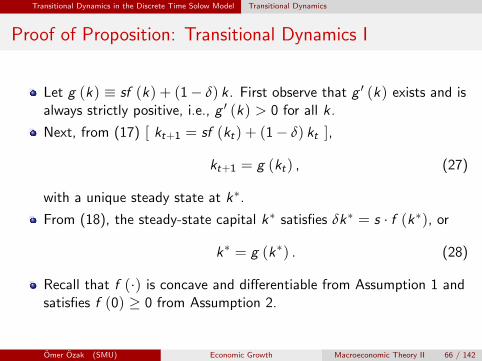
Let g (k) ≡ sf (k) + (1− δ) k. First observe that g ′ (k) exists and isalways strictly positive, i.e., g ′ (k) > 0 for all k .
Next, from (17) [ kt+1 = sf (kt) + (1− δ) kt ],
kt+1 = g (kt) , (27)
with a unique steady state at k∗.
From (18), the steady-state capital k∗ satisfies δk∗ = s · f (k∗), or
k∗ = g (k∗) . (28)
Recall that f (·) is concave and differentiable from Assumption 1 andsatisfies f (0) ≥ 0 from Assumption 2.
Omer Ozak (SMU) Economic Growth Macroeconomic Theory II 66 / 142

Transitional Dynamics in the Discrete Time Solow Model Transitional Dynamics
Proof of Proposition: Transitional Dynamics II
For any strictly concave differentiable function,
f (k) > f (0) + kf ′ (k) ≥ kf ′ (k) , (29)
The second inequality uses the fact that f (0) ≥ 0.
Since (29) implies that δ = sf (k∗) /k∗ > sf ′ (k∗), we haveg ′ (k∗) = sf ′ (k∗) + 1− δ < 1. Therefore,
g ′ (k∗) ∈ (0, 1) .
The Simple Result then establishes local asymptotic stability.
Omer Ozak (SMU) Economic Growth Macroeconomic Theory II 67 / 142
Transitional Dynamics in the Discrete Time Solow Model Transitional Dynamics
Proof of Proposition: Transitional Dynamics III
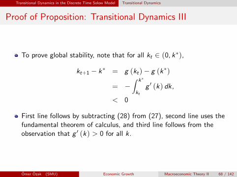
To prove global stability, note that for all kt ∈ (0, k∗),
kt+1 − k∗ = g (kt)− g (k∗)
= −∫ k∗
ktg ′ (k) dk,
< 0
First line follows by subtracting (28) from (27), second line uses thefundamental theorem of calculus, and third line follows from theobservation that g ′ (k) > 0 for all k .
Omer Ozak (SMU) Economic Growth Macroeconomic Theory II 68 / 142

Transitional Dynamics in the Discrete Time Solow Model Transitional Dynamics
Proof of Proposition: Transitional Dynamics IV
Next, (17) also implies
kt+1 − ktkt
= sf (kt)
kt− δ
> sf (k∗)
k∗− δ
= 0,
Second line uses the fact that f (k) /k is decreasing in k (from (29)above) and last line uses the definition of k∗.
These two arguments together establish that for all kt ∈ (0, k∗),kt+1 ∈ (kt , k∗).
An identical argument implies that for all kt > k∗, kt+1 ∈ (k∗, kt).
Therefore, {kt}∞t=0 monotonically converges to k∗ and is globally
stable.
Omer Ozak (SMU) Economic Growth Macroeconomic Theory II 69 / 142

Transitional Dynamics in the Discrete Time Solow Model Transitional Dynamics
Transitional Dynamics in the Discrete Time Solow Model II
Stability result can be seen diagrammatically in the Figure:
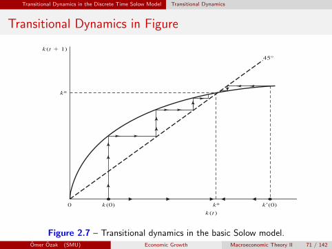
Starting from initial capital stock k (0) < k∗, economy grows towardsk∗, capital deepening and growth of per capita income.If economy were to start with k ′ (0) > k∗, reach the steady state bydecumulating capital and contracting.
Proposition (6) Suppose that Assumptions 1 and 2 hold, and k (0) < k∗,then {wt}∞
t=0 is an increasing sequence and {Rt}∞t=0 is a
decreasing sequence. If k (0) > k∗, the opposite resultsapply.
Thus far Solow growth model has a number of nice properties, but nogrowth, except when the economy starts with k (0) < k∗.
Omer Ozak (SMU) Economic Growth Macroeconomic Theory II 70 / 142
Transitional Dynamics in the Discrete Time Solow Model Transitional Dynamics
Transitional Dynamics in Figure2.4 The Solow Model in Continuous Time . 47
0 k*k(0) k�(0)
k(t)
k(t � 1)
k*
45°
FIGURE 2.7 Transitional dynamics in the basic Solow model.
Recall that when the economy starts with too little capital relative to its labor supply,the capital-labor ratio will increase. Thus the marginal product of capital will fall due todiminishing returns to capital and the wage rate will increase. Conversely, if it starts withtoo much capital, it will decumulate capital, and in the process the wage rate will decline andthe rate of return to capital will increase.
The analysis has established that the Solow growth model has a number of nice properties:unique steady state, global (asymptotic) stability, and finally, simple and intuitive comparativestatics. Yet so far it has no growth. The steady state is the point at which there is no growthin the capital-labor ratio, no more capital deepening, and no growth in output per capita.Consequently, the basic Solow model (without technological progress) can only generateeconomic growth along the transition path to the steady state (starting with k(0) < k∗). Howeverthis growth is not sustained: it slows down over time and eventually comes to an end. Section2.7 shows that the Solow model can incorporate economic growth by allowing exogenoustechnological change. Before doing this, it is useful to look at the relationship between thediscrete- and continuous-time formulations.
2.4 The Solow Model in Continuous Time
2.4.1 From Difference to Differential Equations
Recall that the time periods t = 0, 1, . . . can refer to days, weeks, months, or years. In somesense, the time unit is not important. This arbitrariness suggests that perhaps it may be moreconvenient to look at dynamics by making the time unit as small as possible, that is, by goingto continuous time. While much of modern macroeconomics (outside of growth theory) uses
Figure 2.7 – Transitional dynamics in the basic Solow model.
————————————
Omer Ozak (SMU) Economic Growth Macroeconomic Theory II 71 / 142

The Solow Model in Continuous Time
Section 4
The Solow Model in Continuous Time
Omer Ozak (SMU) Economic Growth Macroeconomic Theory II 72 / 142
The Solow Model in Continuous Time Towards Continuous Time
From Difference to Differential Equations I
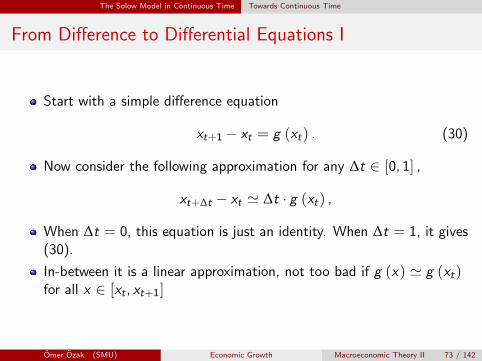
Start with a simple difference equation
xt+1 − xt = g (xt) . (30)
Now consider the following approximation for any ∆t ∈ [0, 1] ,
xt+∆t − xt ' ∆t · g (xt) ,
When ∆t = 0, this equation is just an identity. When ∆t = 1, it gives(30).
In-between it is a linear approximation, not too bad if g (x) ' g (xt)for all x ∈ [xt , xt+1]
Omer Ozak (SMU) Economic Growth Macroeconomic Theory II 73 / 142
The Solow Model in Continuous Time Towards Continuous Time
From Difference to Differential Equations II
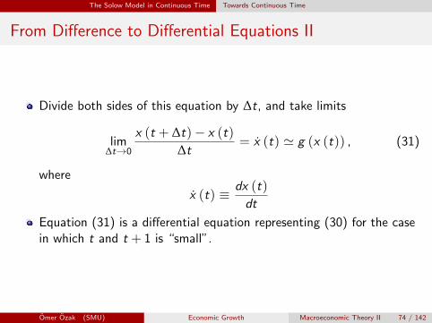
Divide both sides of this equation by ∆t, and take limits
lim∆t→0
x (t + ∆t)− x (t)
∆t= x (t) ' g (x (t)) , (31)
where
x (t) ≡ dx (t)
dt
Equation (31) is a differential equation representing (30) for the casein which t and t + 1 is “small”.
Omer Ozak (SMU) Economic Growth Macroeconomic Theory II 74 / 142

The Solow Model in Continuous Time Steady State in Continuous Time
Fundamental Eq. of Solow Model in Continuous Time I
Nothing has changed on the production side, so (15) still give thefactor prices, now interpreted as instantaneous wage and rental rates.R (t) = f ′ (k (t)) > 0 and w (t) = f (k (t))− k (t) f ′ (k (t)) > 0.
Savings are again: S (t) = sY (t) ,
Consumption is given by (11) above: C (t) = (1− s)Y (t)
Omer Ozak (SMU) Economic Growth Macroeconomic Theory II 75 / 142
The Solow Model in Continuous Time Steady State in Continuous Time
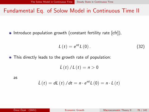
Fundamental Eq. of Solow Model in Continuous Time II
Introduce population growth (constant fertility rate [cfr]),
L (t) = entL (0) . (32)
This directly leads to the growth rate of population:
L (t) /L (t) = n > 0
asL (t) = dL (t) /dt = n · entL (0) = n · L (t)
Omer Ozak (SMU) Economic Growth Macroeconomic Theory II 76 / 142
The Solow Model in Continuous Time Steady State in Continuous Time
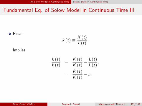
Fundamental Eq. of Solow Model in Continuous Time III
Recall
k (t) ≡ K (t)
L (t),
Implies
k (t)
k (t)=
K (t)
K (t)− L (t)
L (t),
=K (t)
K (t)− n.
Omer Ozak (SMU) Economic Growth Macroeconomic Theory II 77 / 142

The Solow Model in Continuous Time Steady State in Continuous Time
Fundamental Eq. of Solow Model in Continuous Time IV
From the limiting argument leading to equation (31),
K (t) = sF [K (t) , L (t) ,A (t)]− δK (t) .
Using the definition of k (t) and the constant returns to scaleproperties of the production function,
k (t)
k (t)= s
F [K , L,A]
K (t)− (n+ δ) = s
f (k (t))
k (t)− (n+ δ) , (33)
Omer Ozak (SMU) Economic Growth Macroeconomic Theory II 78 / 142
The Solow Model in Continuous Time Steady State in Continuous Time
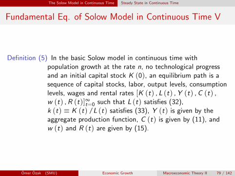
Fundamental Eq. of Solow Model in Continuous Time V
Definition (5) In the basic Solow model in continuous time withpopulation growth at the rate n, no technological progressand an initial capital stock K (0), an equilibrium path is asequence of capital stocks, labor, output levels, consumptionlevels, wages and rental rates [K (t) , L (t) ,Y (t) ,C (t) ,w (t) ,R (t)]∞t=0 such that L (t) satisfies (32),k (t) ≡ K (t) /L (t) satisfies (33), Y (t) is given by theaggregate production function, C (t) is given by (11), andw (t) and R (t) are given by (15).
Omer Ozak (SMU) Economic Growth Macroeconomic Theory II 79 / 142
The Solow Model in Continuous Time Steady State in Continuous Time
Fundamental Eq. of Solow Model in Continuous Time VI
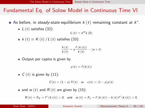
As before, in steady-state equilibrium k (t) remaining constant at k∗.
L (t) satisfies (32):L (t) = entL (0)
k (t) ≡ K (t) /L (t) satisfies (33):
k (t)
k (t)= s
f (k (t))
k (t)− (n+ δ)
Output per capita is given by
y (t) = f (k(t))
C (t) is given by (11):
C (t) = (1− s)Y (t) or c(t) = (1− s)y (t)
and w (t) and R (t) are given by (15):
R (t) = FK = f ′ (k (t)) > 0 and w (t) = FL = f (k (t))− k (t) f ′ (k (t)) > 0.
Omer Ozak (SMU) Economic Growth Macroeconomic Theory II 80 / 142
The Solow Model in Continuous Time Steady State in Continuous Time
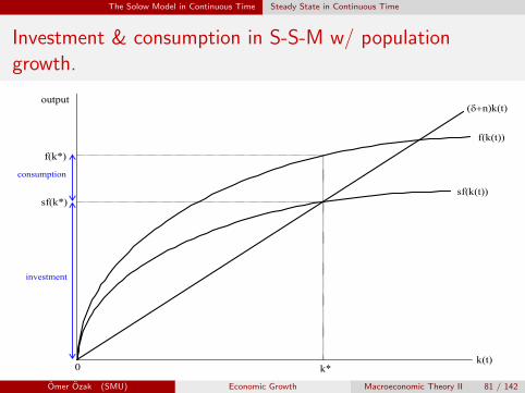
Investment & consumption in S-S-M w/ populationgrowth.
Introduction to Modern Economic Growth
output
k(t)
f(k*)
k*
f(k(t))
sf(k*)sf(k(t))
consumption
investment
0
(δ+n)k(t)
Figure 2.8. Investment and consumption in the state-state equilib-rium with population growth.
Proposition 2.7. Consider the basic Solow growth model in continuous time
and suppose that Assumptions 1 and 2 hold. Then there exists a unique steady state
equilibrium where the capital-labor ratio is equal to k∗ ∈ (0,∞) and is given by(2.33), per capita output is given by
y∗ = f (k∗)
and per capita consumption is given by
c∗ = (1− s) f (k∗) .
Moreover, again defining f (k) = af (k) , we have (proof omitted):
70
Figure 2.8 – Investment & consumption in the steady-state equilibrium with population growth.Omer Ozak (SMU) Economic Growth Macroeconomic Theory II 81 / 142
The Solow Model in Continuous Time Steady State in Continuous Time
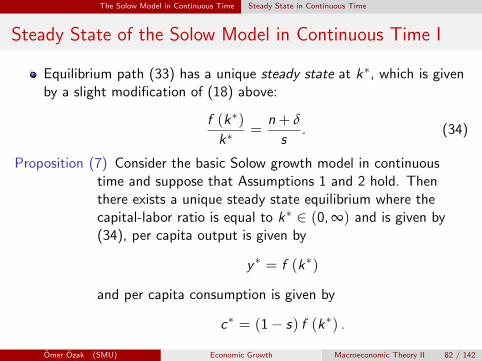
Steady State of the Solow Model in Continuous Time I
Equilibrium path (33) has a unique steady state at k∗, which is givenby a slight modification of (18) above:
f (k∗)
k∗=
n+ δ
s. (34)
Proposition (7) Consider the basic Solow growth model in continuoustime and suppose that Assumptions 1 and 2 hold. Thenthere exists a unique steady state equilibrium where thecapital-labor ratio is equal to k∗ ∈ (0, ∞) and is given by(34), per capita output is given by
y ∗ = f (k∗)
and per capita consumption is given by
c∗ = (1− s) f (k∗) .
Omer Ozak (SMU) Economic Growth Macroeconomic Theory II 82 / 142

The Solow Model in Continuous Time Steady State in Continuous Time
Steady State of the Solow Model in Continuous Time II
Moreover, again defining f (k) = Af (k) , we obtain:
Proposition (8) Suppose Assumptions 1 and 2 hold and f (k) = Af (k).Denote the steady-state equilibrium level of the capital-laborratio by k∗ (A, s, δ, n) and the steady-state level of output byy ∗ (A, s, δ, n) when the underlying parameters are given byA, s and δ. Then we have
∂k∗ (·)∂A
> 0,∂k∗ (·)
∂s> 0,
∂k∗ (·)∂δ
< 0 and∂k∗ (·)
∂n< 0
∂y ∗ (·)∂A
> 0,∂y ∗ (·)
∂s> 0,
∂y ∗ (·)∂δ
< 0 and∂y ∗ (·)
∂n< 0.
Omer Ozak (SMU) Economic Growth Macroeconomic Theory II 83 / 142

The Solow Model in Continuous Time Steady State in Continuous Time
Steady State of the Solow Model in Continuous Time III
Relative to the earlier n = 0 (Prop. 3) a higher population growthrate, n > 0, reduces the capital-labor ratio and output per capita.
n > 0 → faster dilution of capital → lower SS capital-labor ratio.
Testable Implication:
countries with high population growth rates should be poorer.
Omer Ozak (SMU) Economic Growth Macroeconomic Theory II 84 / 142

Transitional Dynamics in the Continuous Time Solow Model
Section 5
Transitional Dynamics in the Continuous Time SolowModel
Omer Ozak (SMU) Economic Growth Macroeconomic Theory II 85 / 142
Transitional Dynamics in the Continuous Time Solow Model Dynamics in Continues Time
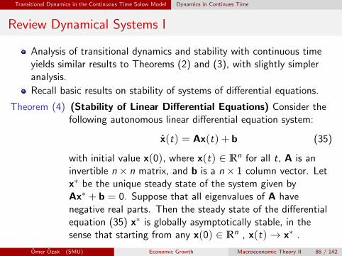
Review Dynamical Systems I
Analysis of transitional dynamics and stability with continuous timeyields similar results to Theorems (2) and (3), with slightly simpleranalysis.
Recall basic results on stability of systems of differential equations.
Theorem (4) (Stability of Linear Differential Equations) Consider thefollowing autonomous linear differential equation system:
x(t) = Ax(t) + b (35)
with initial value x(0), where x(t) ∈ Rn for all t, A is aninvertible n× n matrix, and b is a n× 1 column vector. Letx∗ be the unique steady state of the system given byAx∗ + b = 0. Suppose that all eigenvalues of A havenegative real parts. Then the steady state of the differentialequation (35) x∗ is globally asymptotically stable, in thesense that starting from any x(0) ∈ Rn , x(t)→ x∗ .
Omer Ozak (SMU) Economic Growth Macroeconomic Theory II 86 / 142
Transitional Dynamics in the Continuous Time Solow Model Dynamics in Continues Time
Review Dynamical Systems II
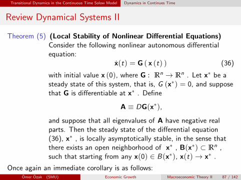
Theorem (5) (Local Stability of Nonlinear Differential Equations)Consider the following nonlinear autonomous differentialequation:
x(t) = G ( x (t) ) (36)
with initial value x (0), where G : Rn → Rn . Let x∗ be asteady state of this system, that is, G (x∗) = 0, and supposethat G is differentiable at x∗ . Define
A ≡ DG(x∗),
and suppose that all eigenvalues of A have negative realparts. Then the steady state of the differential equation(36), x∗ , is locally asymptotically stable, in the sense thatthere exists an open neighborhood of x∗ , B(x∗) ⊂ Rn ,such that starting from any x(0) ∈ B(x∗), x(t)→ x∗ .
Once again an immediate corollary is as follows:Omer Ozak (SMU) Economic Growth Macroeconomic Theory II 87 / 142

Transitional Dynamics in the Continuous Time Solow Model Dynamics in Continues Time
Review Dynamical Systems III
Corollary (2) 1 Let x(t) ∈ R. Then the steady state of the lineardifferential equation x(t) = ax(t) + b is asymptoticallyglobally stable (in the sense that x(t)→ −b/a) ifa < 0.
2 Let g : R→ R be differentiable in the neighborhood ofthe steady state x∗ defined by g(x∗) = 0 and supposethat g ′(x∗) < 0. Then the steady state of the nonlineardifferential equation x(t) = g(x(t)) , x∗ , is locallyasymptotically stable.
Omer Ozak (SMU) Economic Growth Macroeconomic Theory II 88 / 142
Transitional Dynamics in the Continuous Time Solow Model Dynamics in Continues Time
Transitional Dynamics Continuous Time Solow Model I
Simple Result about Stability In Continuous Time Model
Let g : R→ R be a differentiable function and suppose that thereexists a unique x∗ such that g (x∗) = 0.
Moreover, suppose g (x) < 0 for all x > x∗ and g (x) > 0 for allx < x∗.Then the steady state of the nonlinear differential equationx (t) = g (x (t)), x∗, is globally asymptotically stable, i.e., startingwith any x (0), x (t)→ x∗.
Note that g(x) could be non-monotonic and still satisfy the first condition.
Omer Ozak (SMU) Economic Growth Macroeconomic Theory II 89 / 142

Transitional Dynamics in the Continuous Time Solow Model Dynamics in Continues Time
Dynamics of capital-labor ratio in basic Solow model52 . Chapter 2 The Solow Growth Model
0k*
k(t)
k(t)·
k(t)
� (• � g � n)sf(k(t))
k(t)
FIGURE 2.9 Dynamics of the capital-labor ratio in the basic Solow model.
Notice that the equivalent of part 3 of Corollary 2.2 is not true in discrete time. Theimplications of this observation are illustrated in Exercise 2.21.
In view of these results, Proposition 2.5 has a straightforward generalization of the resultsfor discrete time.
Proposition 2.9 Suppose that Assumptions 1 and 2 hold. Then the basic Solow growthmodel in continuous time with constant population growth and no technological change isglobally asymptotically stable and, starting from any k(0) > 0, k(t) monotonically convergesto k∗.
Proof. The proof of stability is now simpler and follows immediately from part 3 of Corol-lary 2.2 by noting that when k < k∗, we have sf (k) − (n + δ)k > 0, and when k > k∗, we havesf (k) − (n + δ)k < 0.
Figure 2.9 shows the analysis of stability diagrammatically. The figure plots the right-handside of (2.33) and makes it clear that when k < k∗, k > 0, and when k > k∗, k < 0, so that thecapital-labor ratio monotonically converges to the steady-state value k∗.
Example 2.2 (Dynamics with the Cobb-Douglas Production Function) Let us returnto the Cobb-Douglas production function introduced in Example 2.1:
F(K, L, A) = AKαL1−α, with 0 < α < 1.
As noted above, the Cobb-Douglas production function is special, mainly because it has anelasticity of substitution between capital and labor equal to 1. For a homothetic productionfunction F(K, L), the elasticity of substitution is defined by
σ ≡ −[∂ log(FK/FL)
∂ log(K/L)
]−1
, (2.37)
Figure 2.9 – Dynamics of the capital-labor ratio in the basic Solow model. – Simple Result.Omer Ozak (SMU) Economic Growth Macroeconomic Theory II 90 / 142
Transitional Dynamics in the Continuous Time Solow Model Dynamics in Continues Time
Transitional Dynamics Continuous Time Solow Model II
Fundamental equation is
k (t) = s · f (k (t))− (n+ δ) k (t) ,
so that
∂k (t)
∂k (t)= s · f ′ (k (t))− (n+ δ) .
Thus, SS is determined by
s · f (k∗) = (n+ δ) k∗ → (n+ δ) = s · f (k∗) /k∗
taking derivative wrt k∗
∂k
∂k(k∗) = s · f ′ (k∗)− (n+ δ) = s · f ′ (k∗)− s · f (k∗) /k∗
Omer Ozak (SMU) Economic Growth Macroeconomic Theory II 91 / 142
Transitional Dynamics in the Continuous Time Solow Model Dynamics in Continues Time
Transitional Dynamics Continuous Time Solow Model III
Using the SS condition, we have that
∂k
∂k(k∗) = s ·
[f ′ (k∗) k∗ − s · f (k∗)
k∗
]= − s · w ∗
k∗< 0
i.e.
∂k (k∗)
∂k< 0.
Omer Ozak (SMU) Economic Growth Macroeconomic Theory II 92 / 142
Transitional Dynamics in the Continuous Time Solow Model Dynamics in Continues Time
Transitional Dynamics Continuous Time Solow Model VII
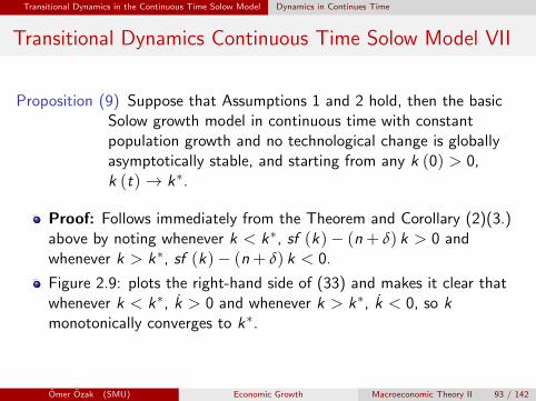
Proposition (9) Suppose that Assumptions 1 and 2 hold, then the basicSolow growth model in continuous time with constantpopulation growth and no technological change is globallyasymptotically stable, and starting from any k (0) > 0,k (t)→ k∗.
Proof: Follows immediately from the Theorem and Corollary (2)(3.)above by noting whenever k < k∗, sf (k)− (n+ δ) k > 0 andwhenever k > k∗, sf (k)− (n+ δ) k < 0.
Figure 2.9: plots the right-hand side of (33) and makes it clear thatwhenever k < k∗, k > 0 and whenever k > k∗, k < 0, so kmonotonically converges to k∗.
Omer Ozak (SMU) Economic Growth Macroeconomic Theory II 93 / 142
Transitional Dynamics in the Continuous Time Solow Model Cobb-Douglas Example
Dynamics with Cobb-Douglas Production Function I
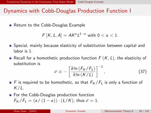
Return to the Cobb-Douglas Example
F [K , L,A] = AK αL1−α with 0 < α < 1.
Special, mainly because elasticity of substitution between capital andlabor is 1.
Recall for a homothetic production function F (K , L), the elasticity ofsubstitution is
σ ≡ −[
∂ ln (FK/FL)∂ ln (K/L)
]−1
, (37)
F is required to be homothetic, so that FK/FL is only a function ofK/L.
For the Cobb-Douglas production functionFK/FL = (α/ (1− α)) · (L/K ), thus σ = 1.
Omer Ozak (SMU) Economic Growth Macroeconomic Theory II 94 / 142

Transitional Dynamics in the Continuous Time Solow Model Cobb-Douglas Example
Dynamics with Cobb-Douglas Production Function II
When the production function is Cobb-Douglas and factor marketsare competitive, equilibrium factor shares will be constant:
αK (t) =R (t)K (t)
Y (t)
=FK (K (t), L (t))K (t)
Y (t)
=αA [K (t)]α−1 [L (t)]1−α K (t)
A [K (t)]α [L (t)]1−α
= α.
Similarly, the share of labor is αL (t) = 1− α.
Reason: with σ = 1, as capital increases, its marginal productdecreases proportionally, leaving the capital share constant.
Omer Ozak (SMU) Economic Growth Macroeconomic Theory II 95 / 142

Transitional Dynamics in the Continuous Time Solow Model Cobb-Douglas Example
Dynamics with Cobb-Douglas Production Function III
Per capita production function takes the form f (k) = Akα, so thesteady state is given again as
A (k∗)α−1 =n+ δ
sor
k∗ =
(sA
n+ δ
) 11−α
,
k∗ is increasing in s and A and decreasing in n and δ.In addition, k∗ is increasing in α: higher α implies higher share paidto capital and less diminishing MPKTransitional dynamics are also straightforward in this case:
k (t) = sA [k (t)]α − (n+ δ) k (t)
with initial condition k (0).
Omer Ozak (SMU) Economic Growth Macroeconomic Theory II 96 / 142

Transitional Dynamics in the Continuous Time Solow Model Cobb-Douglas Example
Dynamics with Cobb-Douglas Production Function IV
To solve this equation, let x (t) ≡ k (t)1−α,
x (t) = (1− α) sA− (1− α) (n+ δ) x (t) ,
General solution
x (t) =sA
n+ δ+
[x (0)− sA
n+ δ
]exp (− (1− α) (n+ δ) t) .
In terms of the capital-labor ratio
k (t) =
{sA
n+ δ+
[[k (0)]1−α − sA
n+ δ
]exp (− (1− α) (n+ δ) t)
} 11−α
.
Omer Ozak (SMU) Economic Growth Macroeconomic Theory II 97 / 142
Transitional Dynamics in the Continuous Time Solow Model Cobb-Douglas Example
Dynamics with Cobb-Douglas Production Function V
This solution illustrates:
starting from any k (0), k (t)→ k∗ = (sA/ (n+ δ))1/(1−α), and rateof adjustment is related to (1− α) (n+ δ),more specifically, gap between k (0) and its steady-state value is closedat the exponential rate (1− α) (n+ δ).
Intuitive:
higher α, less diminishing returns, slows down rate at which marginaland average product of capital declines, reduces rate of adjustment tosteady state.smaller δ and smaller n: slow down the adjustment of capital perworker and thus the rate of transitional dynamics.
Omer Ozak (SMU) Economic Growth Macroeconomic Theory II 98 / 142

Transitional Dynamics in the Continuous Time Solow Model Constant Elasticity of Substitution Example
Constant Elasticity of Substitution Production Function I
Constant Elasticity of Substitution – CES
Imposes a constant elasticity, σ, not necessarily equal to 1.
Consider a vector-valued index of technologyA (t) = (AH (t) ,AK (t) ,AL (t)).CES production function can be written as
Y (t) = F [K (t) , L (t) , A (t)]
≡ AH (t)[γ (AK (t)K (t))
σ−1σ + (1− γ) (AL (t) L (t))
σ−1σ
] σσ−1
,(38)
AH (t) > 0, AK (t) > 0 and AL (t) > 0 are three different types oftechnological change
γ ∈ (0, 1) is a distribution parameter,
Omer Ozak (SMU) Economic Growth Macroeconomic Theory II 99 / 142

Transitional Dynamics in the Continuous Time Solow Model Constant Elasticity of Substitution Example
Constant Elasticity of Substitution Production Function II
σ ∈ [0, ∞] is the elasticity of substitution: easy to verify that
FKFL
=γAK (t)
σ−1σ K (t)−
1σ
(1− γ)AL (t)σ−1
σ L (t)−1σ
,
Thus, indeed have
σ = −[
∂ ln (FK/FL)∂ ln (K/L)
]−1
.
Omer Ozak (SMU) Economic Growth Macroeconomic Theory II 100 / 142

Transitional Dynamics in the Continuous Time Solow Model Constant Elasticity of Substitution Example
Constant Elasticity of Substitution Production Function III
As σ→ 1, the CES production function converges to theCobb-Douglas
Y (t) = AH (t) (AK (t))γ (AL (t))1−γ (K (t))γ (L (t))1−γ
As σ→ ∞, the CES production function becomes linear, i.e.
Y (t) = γAH (t)AK (t)K (t) + (1− γ)AH (t)AL (t) L (t) .
Finally, as σ→ 0, the CES production function converges to theLeontief production function with no substitution between factors,
Y (t) = AH (t)min {γAK (t)K (t) ; (1− γ)AL (t) L (t)} .
Leontief production function: if γAK (t)K (t) 6= (1− γ)AL (t) L (t),either capital or labor will be partially “idle”.
Omer Ozak (SMU) Economic Growth Macroeconomic Theory II 101 / 142

A First Look at Sustained Growth
Section 6
A First Look at Sustained Growth
Omer Ozak (SMU) Economic Growth Macroeconomic Theory II 102 / 142

A First Look at Sustained Growth Sustained Growth
A First Look at Sustained Growth I
Cobb-Douglas already showed that when α is close to 1, adjustmentto steady-state level can be very slow.
Simplest model of sustained growth essentially takes α = 1 in termsof the Cobb-Douglas production function above.
Relax Assumptions 1 and 2 and suppose
F [K (t) , L (t) ,A (t)] = AK (t) , (39)
where A > 0 is a constant.
So-called “AK” model, and in its simplest form output does not evendepend on labor.
Results we would like to highlight apply with more general constantreturns to scale production functions, e.g.
F [K (t) , L (t) ,A (t)] = AK (t) + BL (t) , (40)
Omer Ozak (SMU) Economic Growth Macroeconomic Theory II 103 / 142
A First Look at Sustained Growth Sustained Growth
A First Look at Sustained Growth II
Assume population grows at n as before (constant fertility rate [cfr]equation (32)).
Combining with the production function (39),
k (t)
k (t)= sA− δ− n.
Therefore, if sA− δ− n > 0, there will be sustained growth in thecapital-labor ratio.
From (39), this implies that there will be sustained growth in outputper capita as well.
Omer Ozak (SMU) Economic Growth Macroeconomic Theory II 104 / 142

A First Look at Sustained Growth Sustained Growth
A First Look at Sustained Growth III
Proposition (10) Consider the Solow growth model with the productionfunction (39) { F [K (t) , L (t) ,A (t)] = AK (t) }andsuppose that sA− δ− n > 0. Then in equilibrium, there issustained growth of output per capita at the rate sA− δ− n.In particular, starting with a capital-labor ratio k (0) > 0,the economy has
k (t) = exp ((sA− δ− n) t) k (0)
andy (t) = exp ((sA− δ− n) t)Ak (0) .
Note: no transitional dynamics.
Omer Ozak (SMU) Economic Growth Macroeconomic Theory II 105 / 142

A First Look at Sustained Growth Sustained Growth
Sustained Growth in Figure56 . Chapter 2 The Solow Growth Model
0 k(0)
k(t)
k(t � 1)(A � • � n)k(t)
45°
FIGURE 2.10 Sustained growth with the linear AK technology with sA − δ − n > 0.
This proposition not only establishes the possibility of sustained growth but also showsthat when the aggregate production function is given by (2.39), sustained growth is achievedwithout transitional dynamics. The economy always grows at a constant rate sA − δ − n,regardless of the initial level of capital-labor ratio. Figure 2.10 shows this equilibrium dia-grammatically.
Does the AK model provide an appealing approach to explaining sustained growth? Whileits simplicity is a plus, the model has a number of unattractive features. First, it is somewhatof a knife-edge case, which does not satisfy Assumptions 1 and 2; in particular, it requiresthe production function to be ultimately linear in the capital stock. Second and relatedly, thisfeature implies that as time goes by the share of national income accruing to capital will increasetoward 1 (if it is not equal to 1 to start with). The next section shows that this tendency does notseem to be borne out by the data. Finally and most importantly, a variety of evidence suggeststhat technological progress is a major (perhaps the most significant) factor in understanding theprocess of economic growth. A model of sustained growth without technological progress failsto capture this essential aspect of economic growth. Motivated by these considerations, we nextturn to the task of introducing technological progress into the baseline Solow growth model.
2.7 Solow Model with Technological Progress
2.7.1 Balanced Growth
The models analyzed so far did not feature technological progress. I now introduce changesin A(t) to capture improvements in the technological knowhow of the economy. There islittle doubt that today human societies know how to produce many more goods and cando so more efficiently than in the past. The productive knowledge of human society has
Figure 2.10 – Sustained growth with the linear AK technology with sA− δ− n > 0.Omer Ozak (SMU) Economic Growth Macroeconomic Theory II 106 / 142

A First Look at Sustained Growth Sustained Growth
A First Look at Sustained Growth IV
Unattractive features:
1 Knife-edge case, requires the production function to be ultimatelylinear in the capital stock.
2 Implies that as time goes by the share of national income accruing tocapital will increase towards 1. Empirically wages > 0, thus this wouldbe impossible R(t)K (t)/Y (t)→ 1.
3 Technological progress seems to be a major (perhaps the most major)factor in understanding the process of economic growth.
Omer Ozak (SMU) Economic Growth Macroeconomic Theory II 107 / 142

Solow Model with Technological Progress
Section 7
Solow Model with Technological Progress
Omer Ozak (SMU) Economic Growth Macroeconomic Theory II 108 / 142

Solow Model with Technological Progress Balanced Growth
Balanced Growth I
Production function F [K (t) , L (t) ,A (t)] is too general.
May not have balanced growth, i.e. a path of the economy consistentwith the Kaldor facts (Kaldor, 1963). K/Y , r , wL/Y and RK/Yare all (nearly) constants over time.
Kaldor facts:
while output per capita increases, the capital-output ratio, the interestrate, and the distribution of income between capital and labor remainroughly constant.
1 y/y > 0 does not decrease, y grows over time2 k grows over time3 Rt is nearly constant over time4 k/y is nearly constant over time5 wL/Y and RK/Y are nearly constant over time (Cobb-Douglas)6 y/y differs across countries (but not time).
Omer Ozak (SMU) Economic Growth Macroeconomic Theory II 109 / 142

Solow Model with Technological Progress Balanced Growth
Historical Factor Shares2.7 Solow Model with Technological Progress . 57
Capital
Labor
0.0
0.1
0.2
0.3
0.4
0.5
0.6
0.7
0.8
0.9
1.0
Labor and capital share in total value added19
29
1934
1939
1944
1949
1954
1959
1964
1969
1974
1979
1984
1989
1994
1999
FIGURE 2.11 Capital and labor share in the U.S. GDP.
progressed tremendously over the past 200 years, and even more so over the past 1,000 or10,000 years. This suggests that an attractive way of introducing economic growth in theframework developed so far is to allow technological progress in the form of changes in A(t).
The key question is how to model the effects of changes in A(t) on the aggregate productionfunction. The standard approach is to impose discipline on the form of technological progress(and its impact on the aggregate production function) by requiring that the resulting allocationsbe consistent with balanced growth, as defined by the so-called Kaldor facts (Kaldor, 1963).Kaldor noted that while output per capita increases, the capital-output ratio, the interest rate,and the distribution of income between capital and labor remain roughly constant. Figure 2.11,for example, shows the evolution of the shares of capital and labor in the U.S. national income.Throughout the book, balanced growth refers to an allocation where output grows at a constantrate and capital-output ratio, the interest rate, and factor shares remain constant. (Clearly, threeof these four features imply the fourth.)
Figure 2.11 shows that, despite fairly large fluctuations, there is no trend in factor shares.Moreover, a range of evidence suggests that there is no apparent trend in interest rates overlong time horizons (see, e.g., Homer and Sylla, 1991). These facts and the relative constancyof capital-output ratios until the 1970s make many economists prefer models with balancedgrowth to those without. The share of capital in national income and the capital-output ratioare not exactly constant. For example, since the 1970s both the share of capital in nationalincome and the capital-output ratio may have increased, depending on how one measuresthem. Nevertheless, constant factor shares and a constant capital-output ratio provide a goodapproximation to reality and a very useful starting point for our models.
Also for future reference, note that in Figure 2.11 the capital share in national incomeis about 1/3, while the labor share is about 2/3. This estimate ignores the share of land;land is not a major factor of production in modern economies (though this has not been true
Figure 2.11 – Capital and Labor Share in the U.S. GDP.Omer Ozak (SMU) Economic Growth Macroeconomic Theory II 110 / 142

Solow Model with Technological Progress Balanced Growth
Balanced Growth II
Note capital share in national income is about 1/3, while the laborshare is about 2/3.
Ignoring land, not a major factor of production.
But in poor countries land is a major factor of production.
This pattern often makes economists choose AK 1/3L2/3.
Main advantage from our point of view is that balanced growth is thesame as a steady-state in transformed variables
i.e., we will again have k = 0, but the definition of k will change.
But important to bear in mind that growth has many non-balancedfeatures.
e.g., the share of different sectors changes systematically.
Technological progress is Neutral if it does not alter the productionfunction (P/N F/N) in a substantial way.
Omer Ozak (SMU) Economic Growth Macroeconomic Theory II 111 / 142
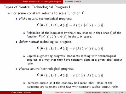
Solow Model with Technological Progress Balanced Growth
Types of Neutral Technological Progress I
For some constant returns to scale function F :
Hicks-neutral technological progress:
F [K (t) , L (t) ,A (t)] = A (t) F [K (t) , L (t)] ,
Relabeling of the Isoquants (without any change in their shape) of thefunction F [K (t) ,L (t) ,A (t)] in the L-K space.
Solow-neutral technological progress,
F [K (t) , L (t) ,A (t)] = F [A (t)K (t) , L (t)] .
Capital-augmenting progress: Isoquants shifting with technologicalprogress in a way that they have constant slope at a given labor-outputratio.
Harrod-neutral technological progress,
F [K (t) , L (t) ,A (t)] = F [K (t) ,A (t) L (t)] .
Increases output as if the economy had more labor: slope of theIsoquants are constant along rays with constant capital-output ratio.
Omer Ozak (SMU) Economic Growth Macroeconomic Theory II 112 / 142
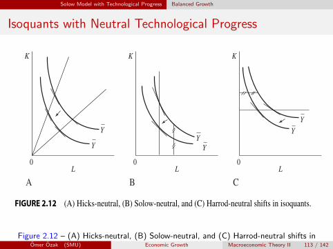
Solow Model with Technological Progress Balanced Growth
Isoquants with Neutral Technological Progress2.7 Solow Model with Technological Progress . 59
0
AL
K
Y
Y
0
BL
K
YY
0
CL
K
Y
Y
FIGURE 2.12 (A) Hicks-neutral, (B) Solow-neutral, and (C) Harrod-neutral shifts in isoquants.
Finally, we can have labor-augmenting or Harrod-neutral technological progress (panel C),named after Roy Harrod (whom we already encountered in the context of the Harrod-Domarmodel):
F (K(t), L(t), A(t)) = F [K(t), A(t)L(t)].
This functional form implies that an increase in technology A(t) increases output as if theeconomy had more labor and thus corresponds to an inward shift of the isoquant as if the laboraxis were being shrunk. The approximate form of the shifts in the isoquants are plotted in thethird panel of Figure 2.12, again for a doubling of A(t).
Of course in practice technological change can be a mixture of these, so we could have avector-valued index of technology A(t) = (
AH(t), AK(t), AL(t))
and a production functionthat looks like
F (K(t), L(t), A(t)) = AH(t)F[AK(t)K(t), AL(t)L(t)
], (2.41)
which nests the CES production function introduced in Example 2.3. Nevertheless, even (2.41)is a restriction on the form of technological progress, since in general changes in technology,A(t), could modify the entire production function.
Although all of these forms of technological progress look equally plausible ex ante, wewill next see that balanced growth in the long run is only possible if all technological progressis labor-augmenting or Harrod-neutral. This result is very surprising and troubling, since thereare no compelling reasons for why technological progress should take this form. I return to adiscussion of why long-run technological change might be Harrod-neutral in Chapter 15.
2.7.3 Uzawa’s Theorem
The discussion above suggests that the key elements of balanced growth are the constancy offactor shares and the constancy of the capital-output ratio, K(t)/Y (t). The shares of capitaland labor in national income are
αK(t) ≡ R(t)K(t)
Y (t)and αL(t) ≡ w(t)L(t)
Y (t).
By Assumption 1 and Theorem 2.1, αK(t) + αL(t) = 1.
Figure 2.12 – (A) Hicks-neutral, (B) Solow-neutral, and (C) Harrod-neutral shifts in
Isoquants.Omer Ozak (SMU) Economic Growth Macroeconomic Theory II 113 / 142

Solow Model with Technological Progress Balanced Growth
Types of Neutral Technological Progress II
Could also have a vector valued index of technologyA (t) = (AH (t) ,AK (t) ,AL (t)) and a production function
F [K (t) , L (t) , A (t)] = AH (t) F [AK (t)K (t) ,AL (t) L (t)] , (41)
Nests the constant elasticity of substitution production functionintroduced in the Example above.
But even (41) is a restriction on the form of technological progress,A (t) could modify the entire production function.
Balanced growth requires that all technological progress be laboraugmenting or Harrod-neutral.
Omer Ozak (SMU) Economic Growth Macroeconomic Theory II 114 / 142

Solow Model with Technological Progress Uzawa’s Theorem
Cobb-Douglas
Under Cobb-Douglas production function these forms are equivalent:
Y (t) = AK (t)α L(t)1−α,
= A1/2[A1/2K (t)
]α [A1/2L (t)
]1−α
=[A1/αK (t)
]αL (t)1−α
= K (t)α[A1/(1−α)L (t)
]1−α: Harrod-neutral used
Focus on continuous time models.
Omer Ozak (SMU) Economic Growth Macroeconomic Theory II 115 / 142

Solow Model with Technological Progress Uzawa’s Theorem
Balanced Growth and Euler
Key elements of balanced growth: constancy of factor shares and ofcapital-output ratio, K (t) /Y (t). By factor shares, we mean:
αL (t) ≡w (t) L (t)
Y (t)and αK (t) ≡ R (t)K (t)
Y (t).
By Assumption 1 and Euler Theorem αL (t) + αK (t) = 1.
All variabes should grow at a constant rate.
Omer Ozak (SMU) Economic Growth Macroeconomic Theory II 116 / 142

Solow Model with Technological Progress Uzawa’s Theorem
Uzawa’s Theorem II
Theorem
(6) (Uzawa I) Suppose L (t) = exp (nt) L (0),
Y (t) = F (K (t) , L (t) , A (t)),
K (t) = Y (t)− C (t)− δK (t), and F is CRS in K and L.Suppose for τ < ∞, Y (t) /Y (t) = gY > 0, K (t) /K (t) = gK > 0 andC (t) /C (t) = gC > 0. Then,
1 gY = gK = gC ; and
2 for any t ≥ τ, F can be represented as
Y (t) = F (K (t) ,A (t) L (t)) ,
where A (t) ∈ R+, F : R2+ → R+ is homogeneous of degree 1, and
A (t) /A (t) = g = gY − n.Omer Ozak (SMU) Economic Growth Macroeconomic Theory II 117 / 142
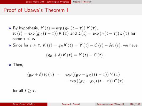
Solow Model with Technological Progress Uzawa’s Theorem
Proof of Uzawa’s Theorem I
By hypothesis, Y (t) = exp (gY (t − τ))Y (τ),K (t) = exp (gK (t − τ))K (τ) and L (t) = exp (n (t − τ)) L (τ) forsome τ < ∞.
Since for t ≥ τ, K (t) = gKK (t) = Y (t)− C (t)− δK (t), we have
(gK + δ)K (t) = Y (t)− C (t) .
Then,
(gK + δ)K (τ) = exp ((gY − gK ) (t − τ))Y (τ)
− exp ((gC − gK ) (t − τ))C (τ)
for all t ≥ τ.
Omer Ozak (SMU) Economic Growth Macroeconomic Theory II 118 / 142
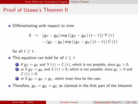
Solow Model with Technological Progress Uzawa’s Theorem
Proof of Uzawa’s Theorem II
Differentiating with respect to time
0 = (gY − gK ) exp ((gY − gK ) (t − τ))Y (τ)
− (gC − gK ) exp ((gC − gK ) (t − τ))C (τ)
for all t ≥ τ.
This equation can hold for all t ≥ τ
1 if gY = gC and Y (τ) = C (τ), which is not possible, since gK > 0.2 or if gY = gK and C (τ) = 0, which is not possible, since gC > 0 and
C (τ) > 0.3 or if gY = gK = gC , which must thus be the case.
Therefore, gY = gK = gC as claimed in the first part of the theorem.
Omer Ozak (SMU) Economic Growth Macroeconomic Theory II 119 / 142
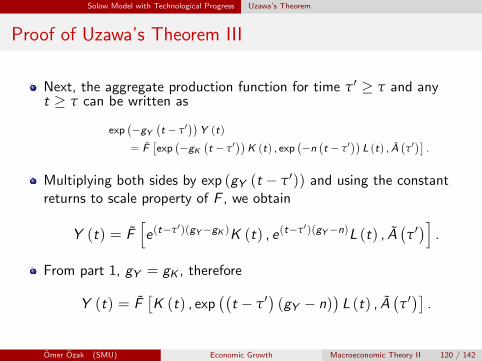
Solow Model with Technological Progress Uzawa’s Theorem
Proof of Uzawa’s Theorem III
Next, the aggregate production function for time τ′ ≥ τ and anyt ≥ τ can be written as
exp(−gY
(t − τ′
))Y (t)
= F[exp
(−gK
(t − τ′
))K (t) , exp
(−n(t − τ′
))L (t) , A
(τ′)]
.
Multiplying both sides by exp (gY (t − τ′)) and using the constantreturns to scale property of F , we obtain
Y (t) = F[e(t−τ′)(gY−gK )K (t) , e(t−τ′)(gY−n)L (t) , A
(τ′)]
.
From part 1, gY = gK , therefore
Y (t) = F[K (t) , exp
((t − τ′
)(gY − n)
)L (t) , A
(τ′)]
.
Omer Ozak (SMU) Economic Growth Macroeconomic Theory II 120 / 142

Solow Model with Technological Progress Uzawa’s Theorem
Proof of Uzawa’s Theorem IV
Moreover, this equation is true for t ≥ τ regardless of τ′, thus
Y (t) = F [K (t) , exp ((gY − n) t) L (t)] ,
= F [K (t) ,A (t) L (t)] ,
withA (t)
A (t)= gY − n
establishing the second part of the theorem.
Omer Ozak (SMU) Economic Growth Macroeconomic Theory II 121 / 142
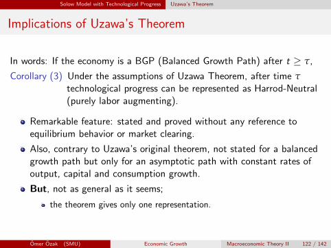
Solow Model with Technological Progress Uzawa’s Theorem
Implications of Uzawa’s Theorem
In words: If the economy is a BGP (Balanced Growth Path) after t ≥ τ,
Corollary (3) Under the assumptions of Uzawa Theorem, after time τtechnological progress can be represented as Harrod-Neutral(purely labor augmenting).
Remarkable feature: stated and proved without any reference toequilibrium behavior or market clearing.
Also, contrary to Uzawa’s original theorem, not stated for a balancedgrowth path but only for an asymptotic path with constant rates ofoutput, capital and consumption growth.
But, not as general as it seems;
the theorem gives only one representation.
Omer Ozak (SMU) Economic Growth Macroeconomic Theory II 122 / 142
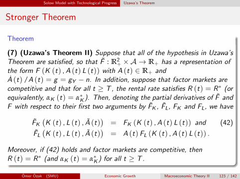
Solow Model with Technological Progress Uzawa’s Theorem
Stronger Theorem
Theorem
(7) (Uzawa’s Theorem II) Suppose that all of the hypothesis in Uzawa’sTheorem are satisfied, so that F : R2
+ ×A → R+ has a representation ofthe form F (K (t) ,A (t) L (t)) with A (t) ∈ R+ andA (t) /A (t) = g = gY − n. In addition, suppose that factor markets arecompetitive and that for all t ≥ T , the rental rate satisfies R (t) = R∗ (orequivalently, αK (t) = α∗K ). Then, denoting the partial derivatives of F andF with respect to their first two arguments by FK , FL, FK and FL, we have
FK(K (t) , L (t) , A (t)
)= FK (K (t) ,A (t) L (t)) and (42)
FL(K (t) , L (t) , A (t)
)= A (t) FL (K (t) ,A (t) L (t)) .
Moreover, if (42) holds and factor markets are competitive, thenR (t) = R∗ (and αK (t) = α∗K ) for all t ≥ T .
Omer Ozak (SMU) Economic Growth Macroeconomic Theory II 123 / 142

Solow Model with Technological Progress Uzawa’s Theorem
Intuition
Suppose the labor-augmenting representation of the aggregateproduction function applies.
Then note that with competitive factor markets, as t ≥ τ,
αK (t) ≡ R (t)K (t)
Y (t)
=K (t)
Y (t)
∂F [K (t) ,A (t) L (t)]
∂K (t)
= α∗K ,
Second line uses the definition of the rental rate of capital in acompetitive market
Third line uses that gY = gK and gK = g + n from Uzawa Theoremand that F exhibits constant returns to scale so its derivative ishomogeneous of degree 0.
Omer Ozak (SMU) Economic Growth Macroeconomic Theory II 124 / 142

Solow Model with Technological Progress Uzawa’s Theorem
Intuition for the Uzawa’s Theorems
We assumed the economy features capital accumulation in the sensethat gK > 0.
From the aggregate resource constraint, this is only possible if outputand capital grow at the same rate.
Either this growth rate is equal to n and there is no technologicalchange (i.e., proposition applies with g = 0), or the economy exhibitsgrowth of per capita income and capital-labor ratio.
The latter case creates an asymmetry between capital and labor:capital is accumulating faster than labor.
Constancy of growth requires technological change to make up forthis asymmetry
But this intuition does not provide a reason for why technologyshould take labor-augmenting (Harrod-neutral) form.
But if technology did not take this form, an asymptotic path withconstant growth rates would not be possible.
Omer Ozak (SMU) Economic Growth Macroeconomic Theory II 125 / 142

Solow Model with Technological Progress Uzawa’s Theorem
Interpretation
Distressing result:
Balanced growth is only possible under a very stringent assumption.Provides no reason why technological change should take this form.
But when technology is endogenous, intuition above also works tomake technology endogenously more labor-augmenting than capitalaugmenting.
Only requires labor augmenting asymptotically, i.e., along thebalanced growth path.
This is the pattern that certain classes of endogenous-technologymodels will generate.
Omer Ozak (SMU) Economic Growth Macroeconomic Theory II 126 / 142

Solow Model with Technological Progress Uzawa’s Theorem
Implications for Modeling of Growth
Does not require Y (t) = F [K (t) ,A (t) L (t)], but only that it has arepresentation of the form Y (t) = F [K (t) ,A (t) L (t)].
Allows one important exception. If (Cobb-Douglas P/N F/N),
Y (t) = [AK (t)K (t)]α [AL(t)L(t)]1−α ,
then both AK (t) and AL (t) could grow asymptotically, whilemaintaining balanced growth.
Because we can define A (t) = [AK (t)]α/(1−α) AL (t) and theproduction function can be represented as
Y (t) = [K (t)]α [A(t)L(t)]1−α .
Differences between labor-augmenting and capital-augmenting (andother forms) of technological progress matter when the elasticity ofsubstitution between capital and labor is not equal to 1.
Omer Ozak (SMU) Economic Growth Macroeconomic Theory II 127 / 142

Solow Model with Technological Progress Uzawa’s Theorem
Further Intuition
Suppose the production function takes the special formF [AK (t)K (t) ,AL (t) L (t)].
The stronger theorem implies that factor shares will be constant.
Given constant returns to scale, this can only be the case whenAK (t)K (t) and AL (t) L (t) grow at the same rate.
The fact that the capital-output ratio is constant in steady state (orthe fact that capital accumulates) implies that K (t) must grow atthe same rate as AL (t) L (t).
Thus balanced growth can only be possible if AK (t) is asymptoticallyconstant.
Omer Ozak (SMU) Economic Growth Macroeconomic Theory II 128 / 142

Solow Model with Technological Progress Solow Growth Model with Technological Progress
The Solow Growth Model with Technological Progress:Continuous Time I
From Uzawa Theorem, production function must admit representationof the form
Y (t) = F [K (t) ,A (t) L (t)] ,
Moreover, supposeA (t)
A (t)= g , (43)
L (t)
L (t)= n.
Again using the constant saving rate
K (t) = sF [K (t) ,A (t) L (t)]− δK (t) . (44)
Omer Ozak (SMU) Economic Growth Macroeconomic Theory II 129 / 142

Solow Model with Technological Progress Solow Growth Model with Technological Progress
The Solow Growth Model with Technological Progress:Continuous Time II
Now define k (t) as the effective capital-labor ratio, i.e.,
k (t) ≡ K (t)
A (t) L (t). (45)
Slight but useful abuse of notation.
Differentiating this expression with respect to time,
k (t)
k (t)=
K (t)
K (t)− g − n. (46)
Output per unit of effective labor can be written as
y (t) ≡ Y (t)
A (t) L (t)= F
[K (t)
A (t) L (t), 1
]≡ f (k (t)) .
Omer Ozak (SMU) Economic Growth Macroeconomic Theory II 130 / 142

Solow Model with Technological Progress Solow Growth Model with Technological Progress
The Solow Growth Model with Technological Progress:Continuous Time III
Income per capita is y (t) ≡ Y (t) /L (t), i.e.,
y (t) = A (t) y (t) (47)
= A (t) f (k (t)) .
Clearly if y (t) is constant, income per capita, y (t), will grow overtime, since A (t) is growing.
Thus should not look for “steady states” where income per capita isconstant, but for balanced growth paths, where income per capitagrows at a constant rate.
Some transformed variables such as y (t) or k (t) in (46) remainconstant.
Thus balanced growth paths can be thought of as steady states of atransformed model.
Omer Ozak (SMU) Economic Growth Macroeconomic Theory II 131 / 142

Solow Model with Technological Progress Solow Growth Model with Technological Progress
The Solow Growth Model with Technological Progress:Continuous Time IV
Hence use the terms “steady state” and balanced growth pathinterchangeably.
Substituting for K (t) from (44) into (46):
k (t)
k (t)=
sF [K (t) ,A (t) L (t)]
K (t)− (δ + g + n) .
Now using (45),
k (t)
k (t)=
sf (k (t))
k (t)− (δ + g + n) , (48)
Only difference is the presence of g : k is no longer the capital-laborratio but the effective capital-labor ratio.
Omer Ozak (SMU) Economic Growth Macroeconomic Theory II 132 / 142

Solow Model with Technological Progress Solow Growth Model with Technological Progress
The Solow Growth Model with Technological Progress:Continuous Time V
Proposition (11) Consider the basic Solow growth model in continuoustime, with Harrod-neutral technological progress at the rateg and population growth at the rate n. Suppose thatAssumptions 1 and 2 hold, and define the effectivecapital-labor ratio as in (45). Then there exists a uniquesteady state (balanced growth path) equilibrium where theeffective capital-labor ratio is equal to k∗ ∈ (0, ∞) and isgiven by
f (k∗)
k∗=
δ + g + n
s. (49)
Per capita output and consumption grow at the rate g .
Omer Ozak (SMU) Economic Growth Macroeconomic Theory II 133 / 142

Solow Model with Technological Progress Solow Growth Model with Technological Progress
The Solow Growth Model with Technological Progress:Continuous Time VI
Equation (49), emphasizes that now total savings, sf (k), are used forreplenishing the capital stock for three distinct reasons:
1 depreciation at the rate δ.2 population growth at the rate n, which reduces capital per worker.3 Harrod-neutral technological progress at the rate g .
Now replenishment of effective capital-labor ratio requiresinvestments to be equal to (δ + g + n) k.
Omer Ozak (SMU) Economic Growth Macroeconomic Theory II 134 / 142
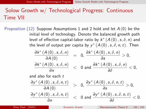
Solow Model with Technological Progress Solow Growth Model with Technological Progress
Solow Growth w/ Technological Progress: ContinuousTime VII
Proposition (12) Suppose Assumptions 1 and 2 hold and let A (0) be theinitial level of technology. Denote the balanced growth pathlevel of effective capital-labor ratio by k∗ (A (0) , s, δ, n) andthe level of output per capita by y ∗ (A (0) , s, δ, n, t). Then
∂k∗ (A (0) , s, δ, n)
∂A (0)= 0,
∂k∗ (A (0) , s, δ, n)
∂s> 0,
∂k∗ (A (0) , s, δ, n)
∂n< 0 and
∂k∗ (A (0) , s, δ, n)
∂δ< 0,
and also for each t
∂y ∗ (A (0) , s, δ, n, t)
∂A (0)> 0,
∂y ∗ (A (0) , s, δ, n, t)
∂s> 0,
∂y ∗ (A (0) , s, δ, n, t)
∂n< 0 and
∂y ∗ (A (0) , s, δ, n, t)
∂δ< 0.
Omer Ozak (SMU) Economic Growth Macroeconomic Theory II 135 / 142

Solow Model with Technological Progress Solow Growth Model with Technological Progress
The Solow Growth Model with Technological Progress:Continuous Time VIII
Proposition (13) Suppose that Assumptions 1 and 2 hold, then the Solowgrowth model with Harrod-neutral technological progress andpopulation growth in continuous time is asymptoticallystable, i.e., starting from any k (0) > 0, the effectivecapital-labor ratio converges to a steady-state value k∗
(k (t)→ k∗).
Now model generates growth in output per capita, but entirelyexogenously.
Omer Ozak (SMU) Economic Growth Macroeconomic Theory II 136 / 142

Comparative Dynamics
Section 8
Comparative Dynamics
Omer Ozak (SMU) Economic Growth Macroeconomic Theory II 137 / 142
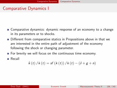
Comparative Dynamics Comparative Dynamics
Comparative Dynamics I
Comparative dynamics: dynamic response of an economy to a changein its parameters or to shocks.
Different from comparative statics in Propositions above in that weare interested in the entire path of adjustment of the economyfollowing the shock or changing parameter.
For brevity we will focus on the continuous time economy.
Recallk (t) /k (t) = sf (k (t)) /k (t)− (δ + g + n)
Omer Ozak (SMU) Economic Growth Macroeconomic Theory II 138 / 142

Comparative Dynamics Comparative Dynamics
Comparative Dynamics in Figure68 . Chapter 2 The Solow Growth Model
0k**
k(t)
k(t)·
k(t)
k*
� (• � g � n)s�f(k(t))
k(t)
� (•� g � n)sf(k(t))
k(t)
FIGURE 2.13 Dynamics following an increase in the saving rate from s to s′. The solid arrows showthe dynamics for the initial steady state, while the dashed arrows show the dynamics for the new steadystate.
comparative dynamics following a one-time, unanticipated, permanent decrease in δ or n areidentical.
The same diagrammatic analysis can be used for studying the effect of an unanticipated buttransitory change in parameters. For example, imagine that s changes in an unanticipatedmanner at t = t ′, but this change will be reversed and the saving rate will return back to itsoriginal value at some known future date t ′′ > t ′. In this case, starting at t ′, the economy followsthe dashed arrows until t ′. After t ′′, the original steady state of the differential equation appliesand together with this, the solid arrows above the horizontal axis become effective. Thus fromt ′′ onward, the economy gradually returns back to its original balanced growth equilibrium, k∗.We will see that similar comparative dynamics can be carried out in the neoclassical growthmodel as well, but the response of the economy to some of these changes will be more complex.
2.9 Taking Stock
What have we learned from the Solow model? At some level, a lot. We now have a simpleand tractable framework that allows us to study capital accumulation and the implications oftechnological progress. As we will see in the next chapter, this framework is already quiteuseful in helping us think about the data.
However, at another level, we have learned relatively little. The questions that Chapter 1posed are related to why some countries are rich while others are poor, why some countriesgrow while others stagnate, and why the world economy embarked upon the process of steadygrowth over the past few centuries. The Solow model shows us that if there is no technological
Figure 2.13 – Dynamics following an increase in the savings rate from s to s ′ . The solid arrows show the dynamics for theinitial steady state, while the dashed arrows show the dynamics for the new steady state.
Omer Ozak (SMU) Economic Growth Macroeconomic Theory II 139 / 142

Comparative Dynamics Comparative Dynamics
Comparative Dynamics II
One-time, unanticipated, permanent increase in the saving rate froms to s ′.
Shifts curve to the right as shown by the dotted line, with a newintersection with the horizontal axis, k∗∗.Arrows on the horizontal axis show how the effective capital-labor ratioadjusts gradually to k∗∗.Immediately, the capital stock remains unchanged (since it is a statevariable).After this point, it follows the dashed arrows on the horizontal axis.
s changes in unanticipated manner at t = t ′ , but will be reversedback to its original value at some known future date t = t ′′ > t ′.
Starting at t ′, the economy follows the rightwards arrows until t ′.After t ′′, the original steady state of the differential equation appliesand leftwards arrows become effective.From t ′′ onwards, economy gradually returns back to its originalbalanced growth equilibrium, k∗.
Omer Ozak (SMU) Economic Growth Macroeconomic Theory II 140 / 142

Conclusions
Section 9
Conclusions
Omer Ozak (SMU) Economic Growth Macroeconomic Theory II 141 / 142
Conclusions
Conclusions
Simple and tractable framework, which allows us to discuss capitalaccumulation and the implications of technological progress.
Solow model shows us that if there is no technological progress, andas long as we are not in the AK world, there will be no sustainedgrowth.
Generate per capita output growth, but only exogenously:technological progress is a black-box.
Capital accumulation: determined by the saving rate, the depreciationrate and the rate of population growth. All are exogenous.
Need to dig deeper and understand what lies in these black boxes.
Omer Ozak (SMU) Economic Growth Macroeconomic Theory II 142 / 142