software engineering for embedded systems || embedded software for networking applications

CHAPTER 24

Embedded Software for NetworkingApplications

Srinivasa Addepalli

Chapter Outline

Introduction 880

System architecture of network devices 881Data, control, service and management planes 882

Multicore SoCs for networking 884Cores 884

Packet engine hardware (PEH) block 885

Parser 886

Distribution 886

Classification 886

Scheduler, queues and channels 886

Accelerators 888

Buffer manager 888

Network programming models 888Pipeline programming model 889

Run-to-completion programming 890

Structure of packet-processing software 891Data-plane infrastructure (DP-Infra) 893

Structure of the forwarding engine 893

Packet-processing application requirements 894

Network application programming techniques 895Multicore performance techniques for network application programmers 895

Avoid locks while looking for flow context 895

Hash table 895

Avoiding locks 897

Avoid reference counting 901

Safe reference mechanism 904

Flow parallelization 906

Reducing cache thrashing associated with updating statistics 910

Statistics acceleration 914

General performance techniques for network application programmers 914Use cache effectively 914

Software-directed prefetching 915

879Software Engineering for Embedded Systems.

DOI: http://dx.doi.org/10.1016/B978-0-12-415917-4.00024-4

© 2013 Elsevier Inc. All rights reserved.

http://dx.doi.org/10.1016/B978-0-12-415917-4.00024-4

Use likely/unlikely compiler built-ins 915

Locking critical piece of code in caches 916

General coding guidelines 916

Linux operating system for embedded network devices 916Translation lookaside buffer (TLB) misses associated with user-space programming 917

Access to hardware peripherals and hardware accelerators 918

Deterministic performance 918

Summary 919

Introduction

Many network appliances are embedded and purpose-built devices. Appliance vendors are

constantly adding multiple functions in devices. These devices support a large number of

protocols to enable LANs (local area networks), WANs (wide area networks) and diverse

networks. Interconnectivity of networks among multiple organizations and enablement of

access to internal resources from external networks such as the Internet are forcing network

devices to be resilient to attacks targeted at them as well as at resources in internal

networks. Due to these factors, embedded software in network devices is no longer simple

and its complexity is reaching the levels of enterprise server application programs.

To mitigate the complexity of device implementations, embedded software developers are

increasingly dependent on general-purpose operating systems such as Linux and NetBSD.

Operating systems provide multiple processing contexts, concurrent programming facilities,

and various abstractions that hide hardware IO devices and accelerators from applications.

These facilities are being used by programmers to develop embedded software faster and to

maintain software easily.

Networks in organizations have migrated from 10 Mbps Ethernet hubs to 100 Mbps.Now

even 1 Gbps Ethernet networks are common. Lately, 10 Gbps Ethernet networks have been

introduced in organizations. In the next few years, one will probably see 40 Gbps and

100 Gbps networks in use. Embedded network devices are expected to handle these rates in

the future. Network device vendors can no longer meet high data traffic rates with single-

core or few-core processors. Instead, they require multicore with many core processors.

However, multicore programming is not simple and getting scalable performance is a very

big challenge that developers face.

This chapter will discuss design and programming considerations in the development of

network applications, with a focus on multicore programming. First, it provides details

on the system architecture of devices. Second, it gives an overview of multicore SoCs.

Third, it introduces some popular network programming models and the structure of

880 Chapter 24

packet-processing applications. Finally, it discusses Linux operating system features that

help in network programming.

Even though this chapter keeps network infrastructure devices in mind while explaining

network programming concepts, these concepts are equally valid for any devices that need

to interact with the external world.

System architecture of network devices

There are many types of network devices one can find in homes, offices and data center

networks. Layer 2 switch devices and to some extent layer 3 switch devices are frequently

seen in many networks. These devices provide high-speed connectivity among end stations

in enterprises, schools, campuses and data centers. Data center networks have many other

devices such as load-balancer devices to balance the traffic across multiple servers in server

farms. There are also network security devices such as firewalls, IP security devices, and

intrusion prevention and detection devices to protect servers from attacks originating from

external networks. All of these devices are called network infrastructure devices and most

of them are embedded and purpose-built.

Before going into the details of the system architecture of network devices, it is important

to refresh some networking concepts. Networking and data communication courses in

colleges and universities teach the open systems interconnection (OSI) model in great

detail. The Internet Protocol Suite, commonly known as TCP/IP, is a set of protocols that

run the Internet. TCP/IP stack protocols implement the first four layers of the OSI model �the physical layer, the data link layer, network layers and the transport layer. The

Transmission Control Protocol of the TCP/IP suite also implements a partial session layer,

the fifth layer of the OSI model, in terms of connection (session) management between

local and remote machines. The Internet Protocol Suite does not implement the session

checkpoint and recovery features of the session layer of the OSI model. The presentation

and application layers of the OSI model are not exactly mapped into any protocol in the

Internet Protocol Suite and are left to applications running on the TCP/IP stack.

The Ethernet protocol is the most prominent physical and data link layer protocol in the

Internet Protocol Suite. Internet Protocol v4 (IPv4) and Internet Protocol v6 (IPv6) are

network layer protocols. The Transmission Control Protocol (TCP), User Datagram Protocol

(UDP), and Stream Control Transmission Protocol (SCTP) are some of the common

transport layer protocols.

All network devices work at different layers of the Internet Protocol suite. L2 switch

devices work at the data link layer, L3 switch devices work at the network layer, load

balancer and security devices typically tend to work at the transport and session layers.

Embedded Software for Networking Applications 881

Though the functionality in these devices is different as they serve different purposes, the

basic system-level architecture of network devices tends to be same. Hence, programming

methods and techniques used to develop network devices tend to be similar in nature.

We believe that understanding the system-level architecture helps developers debug and

maintain software efficiently. Hence the rest of this section provides some details of

high-level software blocks in network devices.

Data, control, service and management planes

Figure 24.1 shows an abstract functional view that many network devices conform to,

which includes data, control, service and management planes.

The data plane, also called the “data path”, is a set of forwarding engines (FE) with each

forwarding engine implementing a function such as L3 routing, IPsec, firewall, etc. The

data plane is the first software component that receives packets from networks using an IO

device such as Ethernet. Each FE is programmed with a set of flow contexts by control and

service planes. Flow context is a memory block which contains information on actions that

are to be taken on the packets, corresponding to a flow.

Any FE, upon receiving a packet, first extracts the packet fields, searches for the matching

flow context and then works on the packet as per the actions in the flow context. Actions

include modification of the packet, information about the next destination of the packet,

Management plane

Data plane

FE 1 FE 2 FE n

Control plane

CE 1 CE 2

CE m

Service plane

SE 1 SE2

SE z

Figure 24.1:System architecture of network devices.

882 Chapter 24

updating statistics counters in the flow context, etc. Data paths are normally updated with

flow contexts by control and service planes. Two different ways in which flow contexts are

updated by control and service planes:

• Reactive updates: control and service plane software engines update flow contexts on

an on-demand basis as part of exception packet processing. When an FE does not find a

matching flow context as part of the packet processing, it sends the packet to the

service plane for further processing. These packets are called exception packets. An

appropriate service plane engine (SE), with the help of configuration information or

information that is negotiated among devices using control plane protocols, determines

the type of actions required and creates a flow context in the right FE.

• Proactive updates: unlike reactive updates, proactive updates are created in data-plane

forwarding engines by service and control planes even before packets hit the device.

Reactive updates are normally associated with inactivity timers. A flow context is

considered inactive if there are no incoming packets matching the flow for a configured

amount of time. The data plane normally removes inactive flows to make room for new

flow contexts. Flow contexts of some forwarding engines are associated with a specific

lifetime too. Flow contexts having a specific lifetime get deleted by the data plane after

living for the time programmed in the context irrespective of packet activity.

Table 24.1 gives the flow context information of some popular forwarding engines.

The service plane contains multiple service engines (SE). Service engines typically process

exception packets coming from forwarding engines, enforce configured policies and update

flow contexts in forwarding engines. For example, the firewall service engine enforces

ACLs (access control lists) created via management engines upon receiving exception

Table 24.1: Flow contexts of some popular forwarding engines.

Forwarding Engine

Key Fields to Find the Matching Flow

Context Important Action Information

L2 bridge/switch Destination MAC address Outbound portL3 router Destination IP address and optionally

source IP address and type of service(ToS)

Outbound interface, gateway IP address,path MTU

L4 forwarding(load balancer,

firewall,NAT etc.)

Source IP address, destination IP address,IP protocol. In the case of TCP and UDPprotocols source port and destination

port are also used as key fields

NAT information on source IP,destination IP, source port, destinationport, TCP sequence number, IP ID etc.

IPsec Inbound tunnel (flow context) isidentified by destination IP address and

SPI (Security Protocol Index)

Key information to decrypt and check theintegrity of the packet


packets. Based on the actions defined in the ACL matching rule, either a flow context is

added in the data plane or the packet is dropped.

The control plane also contains multiple engines called control engines (CEs). CEs typically

implement protocols which interact with peer network devices. The result of control plane

protocols is either directly or indirectly used to create flow contexts in forwarding engines.

In the case of routers, results of OSPF, BGP, RIP, and other routing control plane protocols

are used to create routing flow contexts in the routing forwarding engine. In the case of

IPsec devices, the result of the Internet Key Exchange (IKE) control plane protocol is used

to create the IPsec tunnel contexts in the Ipsec forwarding engine.

The management plane provides human interaction to the network device functionality.

Typical network devices provide multiple management engines, including the command

line interface (CLI), web-based GUIs, SNMP and Netconf.

The performance of network devices is rated in two aspects � throughput of devices and

creation rate of flow contexts. Forwarding engine implementation determines the

throughput and service plane implementation determines the context creation rate. With

increasing traffic in networks and complexity of forwarding engines, throughput and flow

creation rate requirements are going up. Single-core processors are no longer able to

provide the scale that is required. Network equipment vendors are increasingly looking at

multicore processors and SoCs (system-on-chips) to increase the performance of devices.

Thus, embedded system development increasingly requires multicore programming. Before

going into the details of programming models and programming techniques on multicore

processors to implement data and service planes, it is important to have the background on

multicore SoCs. The next section introduces multicore SoCs and the capabilities of these

SoCs that help efficient programming.

Multicore SoCs for networking

The multicore system-on-chip (SoC), as shown in Figure 24.2, consists of multiple general-

purpose cores with multiple peripheral controllers. Multicore SoCs reduce the cost of

network devices as they integrate cores, IO devices (such as Ethernet controllers) and

hardware accelerators (such as crypto, pattern matching and compression accelerators) in a

single die. With multicore SoCs, very few external chips, such as Ethernet phys, DDR, and

flash memory, are required in order to build device hardware boards.

Cores

Multicore SoCs have more than one general-purpose core. MIPS, Power and ARM based

multicore SoCs are common in the market. Many general-purpose operating systems such

884 Chapter 24

as Linux and NetBSD are available on multicore SoCs. Hence, network software developers

can develop networking applications on these cores using general-purpose operating system

programming concepts.

Packet engine hardware (PEH) block

The packet engine is an essential part of multicore SoCs. The PEH works on top of the

Ethernet and interface ports. Its main purpose is to distribute packets across multiple cores,

ensuring that the multiple cores can be utilized for packet processing. Since it is a critical

part in utilizing multiple cores, this section details the capabilities of this block and the

facilities it provides to software.

The PEH provides different schemes to distribute packets across cores. To address the

different requirements of networking applications, PEHs in Multicore SoCs provide various

options for software to control packet distribution. To handle the various types of flow

contexts of different network devices, PEHs provide programmability to distribute the

packets based on a set of header fields. For example, a PEH can be programmed to do

5-tuple (source IP address, destination IP address, IP protocol, source port and destination

port) based packet distribution.

Core Core Core Core Core…

Packet

HW

Engine

Parse, classify,distribute

Scheduler (queues/channels) andcongestion management

Ethernet/other interfaces

QoS

Accelerators

Crypto

Pattern match

Compression

Large scale timer

Figure 24.2:Multicore SoC architecture.


PEHs have the following hardware sub-blocks to enable packet distribution.

Parser

The parser hardware block parses incoming packets from the Ethernet block and extracts

header field values. Parsers have the capability of checking the integrity of the packets �Ethernet CRC validation, IP checksum validation, even transport layer checksum validation

and packet length validations. If a validation of the packet fails, the parser drops the packet.

If all validations are successful, then the parser block proceeds to extract fields from the

packet. Parser sub-blocks also have intelligence to reassemble IP fragments to the full IP

packet. Note that non-initial IP fragments don’t contain the transport header. The parser, to

get hold of transport header fields, reassembles fragments first before it parses the transport

header.

Distribution

The distribution hardware sub-block uses the extracted values of fields to decide on a queue

to place the packet. The distribution hardware applies a hash algorithm on the extracted

fields’ values and uses the hash result to choose one of the queues. CRC-32 and CRC-64

are popular algorithms used by the PEH for calculating hash values. Since all packets

belonging to a flow would result in the same hash value, all packets in the flow would get

placed in the same queue. To facilitate the above, the distribution hardware block provides

facilities for software to program a set of queues and the number of bits from the hash

result.

Classification

The classification hardware block is also used to place incoming packets in queues. This

block provides flexibility for software to assign specific queues to specific flows. As noted

before, the distribution hardware block selects the queues based on the hash result on the

header fields’ values, but does not select queues on specific values of header fields. The

classification hardware block selects the queues based on specific values of fields. As an

example, software can program the classification block to place web GUI (TCP destination

port 80) traffic in a specific queue with different (higher) priority than the queues used by

hash-based distribution. This example configuration would ensure that traffic to port 80 is

given higher priority than other traffic by the PEH scheduler.

Scheduler, queues and channels

Queues and channels are mechanisms used to transfer packets between the PEH and cores.

As discussed above, queues are used by distribution and classification hardware blocks to

place incoming packets. Cores place packets in queues for sending them out or to access

hardware acceleration engines. Queues can also be associated with priority. The distribution

hardware can be programmed to use priority fields in the packet to use different queues in

886 Chapter 24

addition to the hash result. The scheduler block schedules the packets from the queues as

per priority. When a core asks for new work (packet) from the PEH, the scheduler in the

PEH considers the priority of queues first and then uses a round-robin or weighted

round-robin selection mechanism to select a queue from equal-priority queues. Once

the queue is selected, then the packet/work from that queue is given to the requesting

core.

Channels in the PEHs provide a mechanism to bundle a set of queues. They are

typically used if multiple networking software applications require different types of

packets. Consider the case in which an L2 switch application processes packets

belonging to L2 flows coming from some Ethernet ports and an L4 load balancer

processes packets belonging to L4 flows coming from different Ethernet ports. L2 flows

are typically identified based on the “destination MAC address” field of the Ethernet

header, whereas L4 flows are identified based on header fields (5-tuple) from IP and

transport headers. Software, in this case, programs the parser to identify the flows using

the destination MAC address field of packets received on Ethernet ports dedicated to the

L2 switch application. Software also programs the parser to identify the flows using

5-tuples of the packets coming from Ethernet ports associated with the L4 load balancer.

Software also programs distribution hardware with two sets of queues � one set of

queues is used to place the packets corresponding to L2 flows and another set of queues

is used to place the packets of L4 flows. Then software connects each parser

configuration with a set of queues.

The PEH, upon receiving an incoming packet, selects the parser configuration based on the

incoming Ethernet port, extracts relevant fields, calculates a hash on the fields’ values,

identifies the associated queue-set, selects the queue based on the hash result and places the

packet in the queue.

In the above example, two channels are associated with two sets of queues. Cores when

they need a new packet (work) can request the packet from one or more channels. For

example, if some cores are dedicated to the L2 switch application, then these cores would

request work on a channel associated with L2 flows. If some cores are programmed to

handle both L2 and L4 work, then these cores request packets from both channels.

PEHs support many channels to enable development of multiple networking applications on

a device. Schedulers in the PEHs are capable of not only selecting a queue from the set of

queues as part of the de-queue operation by cores, but are also capable of applying a

scheduling algorithm to select a channel.

Essentially, PEHs provide flexibility for software to bundle the packets in flows as required

by applications and distribute the packets of these flows across multiple cores via queues

and channels.


Accelerators

PEHs also include several acceleration blocks to take the load away from the cores on

routine and computationally intensive algorithmic tasks. There are three types of

acceleration engines in PEHs � look-aside accelerators, ingress accelerators, and egress

accelerators.

Look-aside accelerators are the ones used by the software running in cores while processing

the packets. Cryptography, pattern matching, compression/decompression, de-duplication

and timer management are some examples of acceleration units that are normally included

in multicore SoCs.

Ingress acceleration is done by PEHs on the incoming packets before they are handed

over to software running on the cores, in order to save core cycles in certain tasks.

Parsing of headers and making extracted values of header fields available along with the

packets to software is one type of ingress acceleration. Similar to this, some other

popular ingress accelerations in PEHs include packet header integrity checks, reassembly

of IP fragments into full IP packets, aggregation of consecutive TCP segments and

de-tunneling.

Egress acceleration is done by PEMs before transmitting packets to the interfaces. Cores,

after processing the packets, send the packets to the PEH. The PEH then applies actions

before sending them out. Quality of service shaping, link aggregation and tunneling are

some of the acceleration functions that are part of PEHs.

Buffer manager

This is also called the “free pool manager” in the networking industry. Its main purpose is

to maintain free buffer pools. It provides services such as “allocate” and “release”. The

“allocate” operation gets a free buffer from the given buffer pool and the “release”

operation releases the buffer to the pool. Buffer pools are used by the PEH as well as cores.

The PEH uses these pools to allocate buffers to store incoming packets. It frees the buffers

to the pools after transmitting the packets out. Multicore SoCs provide a large number of

buffer pools for software usage too. Software can avoid expensive memory management in

software and can take advantage of these pools.

Network programming models

Network packet-processing applications are normally implemented in two programming

models � the pipeline programming model and the run-to-completion programming

model.

888 Chapter 24

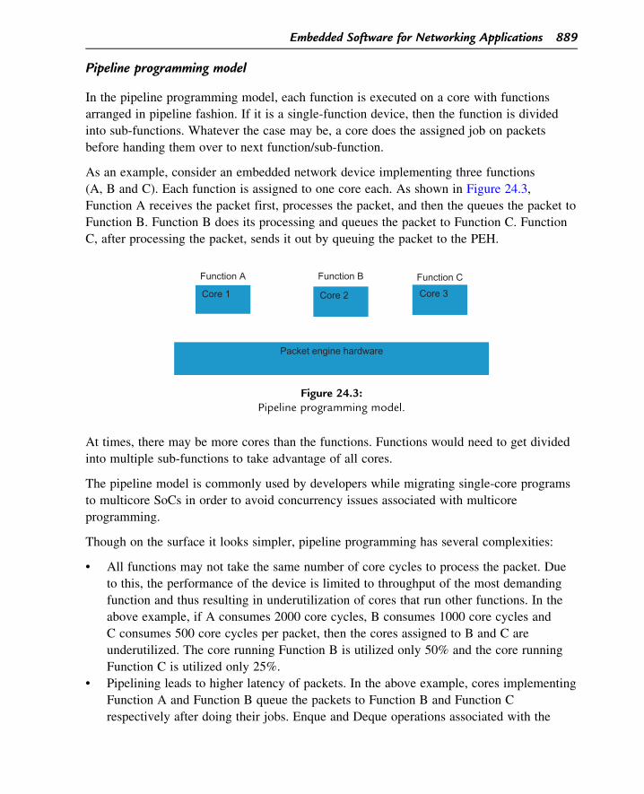
Pipeline programming model

In the pipeline programming model, each function is executed on a core with functions

arranged in pipeline fashion. If it is a single-function device, then the function is divided

into sub-functions. Whatever the case may be, a core does the assigned job on packets

before handing them over to next function/sub-function.

As an example, consider an embedded network device implementing three functions

(A, B and C). Each function is assigned to one core each. As shown in Figure 24.3,

Function A receives the packet first, processes the packet, and then the queues the packet to

Function B. Function B does its processing and queues the packet to Function C. Function

C, after processing the packet, sends it out by queuing the packet to the PEH.

At times, there may be more cores than the functions. Functions would need to get divided

into multiple sub-functions to take advantage of all cores.

The pipeline model is commonly used by developers while migrating single-core programs

to multicore SoCs in order to avoid concurrency issues associated with multicore

programming.

Though on the surface it looks simpler, pipeline programming has several complexities:

• All functions may not take the same number of core cycles to process the packet. Due

to this, the performance of the device is limited to throughput of the most demanding

function and thus resulting in underutilization of cores that run other functions. In the

above example, if A consumes 2000 core cycles, B consumes 1000 core cycles and

C consumes 500 core cycles per packet, then the cores assigned to B and C are

underutilized. The core running Function B is utilized only 50% and the core running

Function C is utilized only 25%.

• Pipelining leads to higher latency of packets. In the above example, cores implementing

Function A and Function B queue the packets to Function B and Function C

respectively after doing their jobs. Enque and Deque operations associated with the

Packet engine hardware

Core 1

Function A

Core 2

Function B

Core 3

Function C

Figure 24.3:Pipeline programming model.


queue management itself use up precious core cycles and also contribute to the latency

of the packets.

• If there are fewer functions than the cores, some functions are to be broken into

multiple sub-functions. This task may not be simple.

Run-to-completion programming

In this programming model, every core processes all functions needed on the packets.

Essentially, the cores run all the functions. All cores receive the packets, process the

packets and send them out as shown in Figure 24.4. In this model, multiple cores receive

the packets from the PEH. This programming model requires PEHs to provide packets from

different flows to different cores. As discussed in the previous section, PEHs can be

programmed to identify flows and queue packets to different queues using hash results

on packet fields. It is very important that only one core processes the packet of any

queue at any time in order to ensure packet ordering within a flow. Networking

applications require maintenance of packet ordering from ingress to egress within a flow.

PEHs can be programmed to block de-queuing of packets from a queue by other cores

if a previous packet from the queue is being processed. The core processing the packet

can signal the PEH to remove the block once it processes the packet. This kind of

handshaking between cores and PEH hardware ensures that the packet ordering is

maintained within a flow.

Since packets belonging to a flow are processed by one core at a time to preserve the

packet ordering, a given flow’s performance is limited to what one core can process. In

typical deployments, there would be a large number of flows and hence multiple cores are

utilized with PEH distributing the flows. If a deployment has fewer flows than cores, then

Core 2

Function A,B,C

Core 1

Function A, B, C

Core N

Function A, B, C


Figure 24.4:Run-to-completion programming model.

890 Chapter 24

some of the cores are underutilized. Though this may seem like a limitation, the run-to-

completion model is accepted in industry since many network deployments have a large

number of simultaneous flows.

Having said that, there could be some instances where a very high throughput is required on

few flows. To utilize the cores effectively, the flows need to be processed by multiple cores

in the pipeline model. To improve performance further, multiple cores can be used at each

pipeline stage. That is, a hybrid model combining run-to-completion and the pipeline model

is required. As shown in Figure 24.5, cores are divided into three pipeline stages where

each stage itself gets implemented in run-to-completion fashion.

The run-to-completion model utilizes multiple cores for a function or set of functions. This

being a popular programming model to implement packet-processing applications, the rest

of the chapter focuses on related programming techniques that programmers need to be

aware of. Multicore programming techniques suitable for network programming are similar

to any multicore programming, with subtle differences. The rest of the chapter focuses on

the structure of packet-processing engines and then describes some important multicore

programming techniques that are useful for packet-processing applications.

Structure of packet-processing software

Data-plane (DP) and service-plane (SP) engines are the main packet-processing engines in

network devices. The structure of packet-processing software whether it is DP or SP

Packet engine

Cores(1,2,3,4)

Function A

Cores (5,6)

Function B,C

Cores (7,8)

Function B,C

Figure 24.5:Hybrid programming model.


software is similar in nature. Though the rest of the chapter mainly uses the term DP and

forwarding engines while describing structure and programming techniques, it is equally

applicable for SP engines too.

Figure 24.6 shows a data plane with multiple forwarding engines (FE1, FE2 to FE N), with

each engine implementing a device function. In the run-to-completion model, FEs call the

next FE by function calls. In the above example, FE1 processes the packet and hands it

over to FE2 by calling a function of FE2. FE2 does its processing and hands over the

packet to the next FE module until the packet is sent out by the last FE (FE N).

• Note: alternative mechanism of calling the next FE: to maintain modularity, many data

path implementations use the approach of functions pointers. Consider an example

where FE1, after processing a packet, needs to select one of the next FEs. Let us also

assume that FE1 uses a packet header field to decide on the next FE to send the packet

to. One approach is to call functions by the name of next FEs based on the value of

field in the packet. Another approach is where neighboring FEs register with function

pointers along with packet field values to the current FE (FE1) at initialization. While

packet processing, FE1 finds the function pointer based on the field value of the current

packet, gets the corresponding function pointer from the registered list and calls the

next FE using the function pointer. This modularity allows new FEs to be added in the

future on top of FE1 without any changes to FE1.

Cores


Data plane common infrastructure(packet/event dispatcher, drivers, utilities)

FE1 FE2 FE N

Figure 24.6:Data-plane architecture.

892 Chapter 24

Data-plane infrastructure (DP-Infra)

Software architects and programmers strive for modularity by dividing the problem into

manageable modules. With increasing complexity of DP implementations due to the large

number of FEs and the complexity of FEs, modularity is required in DP implementations

too. DP-Infra is a set of common modules which are required by DP FEs. By separating out

the common functionality of FEs, it provides several advantages � reusability (hence faster

to add more FEs in future), maintainability, and easy portability of FEs across multiple

different SoCs due to abstraction of the hardware. It is important to understand at this time

that the initial FE (FE1 in above diagram) gets packets from the DP-Infra sub-module.

Similarly, the last FE sends out the packets to the PEH (packet engine hardware) using

DP-Infra. Forwarding engines also interact with the DP-Infra to interact with AEs

(acceleration engines) in PEH.

• Note: this chapter does not get into the details of DP-Infra. At a very high level,

modules in DP-Infra typically include dispatcher, drivers, packet buffer manager, timer

manager, etc. The dispatcher module dispatches packets to requestors � drivers and

FEs. Drivers are software modules that hide details of hardware by providing easy-to-

use API functions for FEs to access hardware accelerators and devices. Packet buffer,

timer and other utilities are mainly easy-to-use library facilities providing consistent

programming methods across FEs. By the way, DP-Infra is typically provided by

multicore SoC vendors as part of their software development kits to jumpstart DP and

SP development on SoCs.

Structure of the forwarding engine

Forwarding engines follow a structure similar to that shown in Figure 24.7. Forwarding

engines receive packets from previous FEs or from the DP-Infra.

First, FEs parse packet headers and extract fields of interest. If it is the first FE receiving

the packets from the PEH, it can use parse results that were extracted by the PEH. As

described earlier, PEHs of multicore SoCs can be programmed to understand the flows and

distribute the flows across cores. PEHs extract fields and values of packet headers to do this

job. The FE receiving packets from PEH can take advantage of PEH parser results.

Second, the flow lookup step, using fields extracted in the previous step, determines the

matching flow context in the flow context database (flow DB). If there is no matching flow,

the packet is sent to the service plane. These packets are called exception packets. As part

of exception packet processing, a flow may be created by the SP in the flow context

database through the flow management module. If there is a matching flow in the database,

then the actual packet processing gets done.


Third, the flow process step processes the packet based on state information in the

flow context. It could result in a new packet, modification of some fields in the packet

header or even dropping the packet. In this step, new state values might be updated in

the flow context. This step also updates statistics. Maintenance of statistics is quite

common in networking applications. Statistics counters such as byte count and packet

count are normally kept on a per flow context basis. There are some counters which

can be updated across the flow contexts and those are called global counters.

Finally, the updated packet is sent out to the next FE. If the current FE is the last module, it

typically sends the packet out using DP-Infra.

Packet-processing application requirements

There are some requirements which developers need to keep in mind while developing an

FE in the run-to-completion model.

• Packet ordering must be preserved in a flow.

• Performance scaling is expected to be almost linear with number of cores assigned to

the data plane.

• Latency of the packet from ingress to egress needs to be kept as small as possible.

Performance scaling is one of the activities developers spend most of their time on, much

more than the time they spend on implementation of data-plane modules. There are two

kinds of performance considerations developers need to keep in mind: multicore-related

performance items and typical programming items.

Packet - in Packet - out

Parse &extract

Flowlookup

FlowmanagementFlow DB

Flow process–modifypacket, update state inflow context, updatestatistics

Operations from sp (flowcreate/delete/modify/query)

Figure 24.7:Structure of forwarding engine.

894 Chapter 24

Network application programming techniques

Multicore performance techniques for network application programmers

Network programmers use a variety of techniques to achieve better performance while

developing packet-processing applications in the DP and the SP.

Locks are used in multicore programming to keep the data integrity in data structures such

as hash tables. Locks ensure that only one core accesses and changes the data structures at

any point in time. This is typically achieved by placing the pieces of code which are

modifying and accessing the data structures under locks. While a core is accessing a data

structure with a lock on it, any other core trying to do any operation on the data structure is

made to spin until the lock is released. Since cores don’t do any useful job during spin, the

performance of packet processing does not scale with multiple cores if there are many locks

in the packet-processing path. Hence networking programmers need to ensure that their

packet-processing code is lock-free as much as possible.

Avoid locks while looking for flow context

Hash table

Packet-processing modules in the DP or SP use various data structures to store flow

contexts. The hash table is one of the most popular data structures used in network

programming. Hence the hash table data structure is used to describe some of the

programming techniques here.

The hash table organization is as shown in Figure 24.8. It is an array of buckets with each

bucket having flow context nodes arranged, typically, in a linked-list fashion. Nodes in the

buckets are also called collision nodes. The hash table, like any other data structure,

Hashbuckets

Flow contextnodes

Figure 24.8:Hash table organization.


provides add, delete and search operations on the nodes. Every hash table is associated with

key parameters. Nodes are added, deleted and searched based on the values of the key

parameters identified for the hash table. For any operation, the hash is calculated first on

the key values. The Bob Jenkins hash algorithm is one of the most popular hash algorithms

used to calculate a hash. Some bits from the hash result are used as the index to the hash

bucket array. Once the bucket is determined, an add operation adds the node to the bucket

linked list either at the head or the tail. A search operation finds the matching node by

doing an exact match on collision nodes. A delete operation deletes the node from the

bucket linked list.

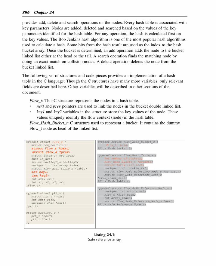
The following set of structures and code pieces provides an implementation of a hash

table in the C language. Though the C structures have many more variables, only relevant

fields are described here. Other variables will be described in other sections of the

document.

Flow_t: This C structure represents the nodes in a hash table.

• next and prev pointers are used to link the nodes in the bucket double linked list.

• key1 and key2 variables in the structure store the key values of the node. These

values uniquely identify the flow context (node) in the hash table.

Flow_Hash_Bucket_t: C structure used to represent a bucket. It contains the dummy

Flow_t node as head of the linked list.

Listing 24.1:Safe reference array.

896 Chapter 24

Flow_Hash_Table_t: this C structure represents the hash table.

• number_of_buckets: indicates the number of buckets in the hash table.

• buckets: array of buckets.

• list_lock: lock used to protect the hash table integrity.

A search operation is issued on the hash table on a per-packet basis in any typical

forwarding engine. Since it is a per-packet operation, the search operation needs to be

very fast in order to achieve good performance. An add operation is executed on the

hash table for every new flow, typically, as part of exception packet processing. A

delete operation is executed to remove a flow upon inactivity or after the life of a flow

has expired. In the run-to-completion programming model, many cores process the

packets and add/delete flows. These operations may happen concurrently. To protect

hash table integrity, locks are required to provide mutually exclusive access to the hash

table.

The search function, as shown in Listing 24.2, takes the table pointer representing the hash

table, hash_key, which is result of a hash function such as the Jenkins hash algorithm on

key values. This function, first, gets the linked list head of the bucket and then does

collision resolution using key1 and key2 fields. Note the statements LOCK_TAKE() and

LOCK_RELEASE(). The LOCK_TAKE function takes the lock. If the lock is already taken

by some other core, then the current core spins until the lock is released by the core that

took the lock. The LOCK_RELEASE function releases the lock. Since cores spin waiting for

the lock, performance does not scale with number of cores if there are more locks and/or if

there is significant code that gets executed under locks.

Avoiding locks

Modern operating systems including Linux support many different types of mutex

functions. Pthreads in Linux supports at least three kinds of mutex primitives � spinlocks

(pthread_spin_lock and pthread_spin_unlock), mutexes (pthread_mutex_lock and

pthread_mutex_unlock) and futexes (fast mutex operations using futex_down and futex_up).

These sets differ in the performance of the mutex operation itself, but the cores stall during

contention in all cases. So, lock-less implementation is the best way to scale the

performance with numbers of cores. Enter the world of Read-Copy-Update (RCU)

primitives.

Read-Copy-Update is a synchronization mechanism supported by many modern operating

systems. It improves the performance of the read-side of a critical section. In the above

example, the search function is a read-side critical section as it does not update the hash

table data structure. Add/Delete functions are write-side critical sections as they update the

data structure. RCU provides wait-free read-side locking and hence many cores can do the

search operation at the same time. Due to this, the packet-processing application


performance can be scaled with the cores. rcu_read_lock() and rcu_read_unlock() are RCU

primitives. These are similar to reader locks, but very fast. In many CPU architectures

supporting in-order instruction execution, RCU read lock/unlock primitives don’t do

Listing 24.2:Search function.

898 Chapter 24

anything really much and are practically stub functions. Even in OOO (out-of-order)

execution-based CPU architectures, these primitives mainly do the “memory bar” (memory

fence) operations and hence are very fast. In some operating systems, lock primitive

disables preemption.

Though the RCU mechanism improves the performance of read operations (search), normal

locks are still required for add/delete operations. Delete operations need additional work

when RCUs are used for read-side protection. A delete operation is expected to postpone

the freeing of a node that is removed from the data structure until all cores have finished

accessing the node. This is achieved by calling synchronize_rcu() or call_rcu() functions

after removing the node from the data structure in the delete operation. synchronize_rcu is a

synchronous operation. Once this function returns, the caller can assume that it is safe to

free the node. call_rcu is an asynchronous operation. This function takes a function pointer

as an argument. This function pointer is called by the RCU infrastructure of the operating

system once the operating system determines that all other cores have finished accessing

the node. The RCU infrastructure calls the callback function pointer once it determines that

all the cores have finished their current execution cycle.

There are two primitives that programmers need to be aware of while using RCUs. They

are rcu_assign_pointer() and rcu_dereference(). rcu_assign_pointer is used to assign new

values to the RCU protected pointer and is needed for readers to see the new value assigned

by the writers. The rcu_deference() primitive is used to get the pointer value from the RCU

protected pointer.

Please see the hash table search, add and delete functions following listings to understand

the usage of RCUs.

A modified search function with RCUs is given in Listing 24.3.

Look at the bold red statement in Listing 24.3. Since the next pointer may be updated by

the add and delete functions, it is necessary to de-reference it using the rcu_dereference()

function. rcu_read_lock and rcu_read_unlock functions are used to showcase the read side

of a critical section of the search operation.

Now let us look at the add and delete functions in Listing 24.4 and Listing 24.5.

Note that the add function still goes with mutex locks. Check the linked-list addition using

rcu_assign_pointer() primitives. rcu_assign_pointer(new_flow-. next, head-. next) is the

same as new_flow-. next 5 head-. next except that head-. next always sees a new

value.

Look at the bold red items in the above listing. A mutex lock is used to protect the critical

section. Since RCU protection is used in the search operation, a flow that is removed from

the hash table should not be freed immediately. The call_rcu function takes the function


pointer and pointer to rcu_head. In the above case, Flow_RCU_free_fn is passed along with

the rcu_head pointer to the call_rcu API function. By defining rcu_head in the flow

context record, it is possible to get the flow context in the Flow_RCU_free_fn(). When

Flow_RCU_free_fn is called by the RCU infrastructure of operating system, the flow is

freed as shown above.

Listing 24.3:Modified search function.

900 Chapter 24

Avoid reference counting

Network packet-processing applications, as discussed, find the matching flow context entry

upon receiving a packet. The flow process step in packet-processing applications refers to

the flow context node multiple times, including accessing and updating state variables and

Listing 24.4:Add operation.


Listing 24.5:Delete operation.

902 Chapter 24

updating statistics. While the flow context record is being accessed, the flow should not be

deleted and freed by any other core. Traditionally this is achieved by applying “reference

counting”.

The reference counting mechanism is typically implemented by two variables in the flow

context records: ref_count and delete_flag. Packet-processing applications normally

increment the reference count of matched flows as part of the search operation. Once the

packet processing is done, the reference count is decremented. A non-zero positive value in

ref_count indicates that the flow is being used by some threads/cores. When a core or a

thread is trying to delete a flow, ref_count is checked first. If it is 0, then the core removes

it from the data structure and frees the flow. If it has a non-zero value, the core/thread

marks the flow for deletion by setting the delete_flag. As cores stop using the flow, they

decrement the ref_count. The last core/thread that de-references the flow (ref_count 55 0)

frees the entry if the flow is marked for deletion. Since there are two variables to implement

the reference count mechanism, locks are used to update or access these two variables

atomically.

There are mainly two issues associated with the reference counting mechanism.

• Locks are required in implementing the reference counting mechanism. Hence, there

would be performance scaling issues with increasing number of cores.

• Error prone: programmers should ensure that the reference count is decremented in

all possible packet paths when the flow is no longer required. While developing

forwarding engines for the first time, programmers might handle this carefully.

But developers may not be as careful or knowledgeable in the code maintenance

phase.

Due to the above issues, programmers are advised to avoid reference counting

mechanisms. The RCU mechanism described above avoids the need for reference

counting. As discussed above, the RCU-based delete operation postpones the freeing-up

of the node until all other threads/cores complete their current run-to-completion cycle.

Therefore any core that is doing the flow process step can be sure of the flow’s

existence until the current run-to-completion cycle is completed. In essence, RCU-based

data structures such as the RCU-based hash table provide two great benefits � avoiding

locks during the flow lookup step and avoiding error-prone reference counting

mechanisms.

There is another reason why the reference counting mechanism is used by programmers. At

times, the neighboring modules need to store the reference to the flow contexts of a

module. Once the reference is stored, the neighbor modules might use the information in

the flows at any time during its processing. If no care is taken, neighbor module might de-

reference the stale pointers of the deleted flows. In the best case, this may lead to accessing


wrong information and in the worst case it may lead to system stability issues. A

reference counting mechanism is used to protect software from these issues. Coding

needs to be done carefully to ensure that ref_count is incremented and decremented at

the right places in neighbor modules. Since the reference counting mechanism is not just

limited to the local module, but extends to neighbor modules, this method is prone to

even more implementation errors. A safe reference method, in addition to RCU, is an

additional technique programmers can use to eliminate the reference counting mechanism

entirely.

Safe reference mechanism

In the reference counting mechanism, neighbor modules store the reference by pointer. In

the safe reference mechanism, neighbor modules store an indirection to the pointer to a

flow context. Indirection happens through an array and includes two important variables �index and cookie. A module that expects a neighbor module to store a reference to its flow

contexts defines a safe reference array data structure in addition to data structures such

as the hash table. As part of the flow context addition operation, the flow context is

not only kept in the hash table, it is also referred from one of the elements in the

safe reference array. Also, a unique cookie is generated upon each addition operation.

This cookie value is also added to the safe reference array element. Please

see Figure 24.9.

Hash table

1235

Pointer to B0

2376

Pointer to A1

2377

Pointer to C2

A B

C

4500

PointerN

Safe reference array

Figure 24.9:Hash table with safe reference array.

904 Chapter 24

The neighbor module is expected to store Index 1 and Cookie 2376 to refer to flow

context A. Since it is no longer a pointer, neighbor modules can’t access the flow

context information directly. The module owning the flow context A provides macros/

API functions for neighbor modules to access any information from flow A. Neighbor

modules are expected to pass safe reference (index and cookie values) to get the needed

information. The module providing the API/macro is expected to check for the validity

of the reference by matching the cookie value given with the cookie value in the safe

reference array. If the cookie values don’t match, it means that the node was deleted

and the module returns an error to the caller. In essence, using safe references instead of

pointers, modules can delete their nodes safely without worrying about neighbor

modules. It not only eliminates the need for reference counting and associated

performance degradation, but it also makes software more modular as it forces neighbor

modules to access information via API/macros.

Listing 24.1 has sr_array in the Flow_Hash_Table_t structure that defines the safe

reference array. The array size is maximum number of nodes supported by that module.

Normally, this array is allocated along with the hash table initialization. free_index_list

maintains the free indices in a linked-list fashion. This helps in finding the free index fast

during flow creation.

Listing 24.1 also has the C structure Flow_Safe_Reference_Node_t, which defines the array

element in the safe reference array. It contains cookie_val and a pointer to the flow context

flow_node. It also has two housekeeping variables � the next pointer is used to maintain

the free_index_list linked list and array_index is to denote the index on the array which this

element represents.

The add operation function listed in Listing 24.4 has logic to populate the safe reference

array element after getting hold of the free array index and the unique cookie value. It gets

the unique cookie value from cookie_val in the hash table, which gets incremented every

time it is used, thereby maintaining uniqueness. Value 0 is reserved to indicate the free

element and hence it avoids using 0 as cookie. Essentially, there is one array element used

for every new flow context. The index to this array element is also stored in the flow to

help in finding the array element from the flow context. Usage of this can be seen from the

delete operation.

if ((free_index 5 Flow_get_free_sr_index(table)) 5 5 0 )

return 0;

if (table-.cookie_val 5 5 0 ) table-.cookie_val11;

table-.sr_array[free_index].cookie_val 5 table-.cookie_val11;

table-.sr_array[free_index].flow_node 5 new_flow;


table-.sr_array[free_index].next 5 NULL;

new_flow-.sr_array_index 5 free_index;

The delete operation function in Listing 24.5 has logic to invalidate the safe reference array

element. The RCU callback function frees the safe reference element to the free linked list.

The following code piece in the Flow_Remove_Node() invalidates the safe reference

element.

array_index 5 flow-.sr_array_index;

table-.sr_array[array_index].cookie_val 5 0;

table-.sr_array[array_index].flow_node 5 NULL;

The following code piece in the Flow_RCU_ free_ fn() puts the safe reference array in the

free linked list.

Flow_free_sr_node(flow-.table, flow-.sr_array_index);

Flow parallelization

The flow parallelization technique allows a flow to be processed by only one core at any

given time. Independent flows are parallelized across cores instead of packet

parallelization, where packets within a flow may get processed by multiple cores

simultaneously. Note that the flow parallelization technique does not bind a flow to a

core permanently. It only ensures that only one core processes any given flow at any

point in time.

Let us see some of the issues with packet parallelization. In packet parallelization mode,

packets are distributed across cores with no consideration to flows. Many forwarding

applications tend to maintain state variables which get updated and accessed during packet

processing. If multiple packets of a flow get processed by more than one core at a time,

then there would be a need to ensure the integrity of state variables in the flow. Mutual

exclusion (a lock) is required to ensure the integrity of state variables. If state variables are

updated or accessed at multiple places during the flow processing step, then more instances

of locking are required to protect these variables. This will reduce the overall performance

of the system.

Many networking applications require packet ordering to be maintained with a flow. If

multiple cores process packets of a flow at the same time, then there is a good possibility of

packet misordering. Note that packet-processing cycles may not be exactly the same across

packets due to various conditions that happen in the system such as core preemption,

interrupt processing, etc. Hence, a newer packet may get processed fast and sent out before

906 Chapter 24

the packet that was received earlier on by some other core. Some applications are very

sensitive to packet order and hence packet ordering is expected to be maintained by packet-

processing applications.

The flow parallelization programming technique is used to overcome the above issues �eliminate locks during the packet-processing path and keep packet order.

As discussed in the section on multicore SoCs in networking, the PEH tries to help in flow

parallelization by bundling packets of a flow into one queue. As long as only one core

processes the queue at a time, flow parallelization is achieved without any special software

programming techniques. The first forwarding engine in the data plane might benefit from

the PEH way of bundling the packets. But software-based flow parallelization is required in

other forwarding engine modules in cases where the granularity or flow definition is

different in these engines. Consider an example of multiple forwarding engines in the

data plane as shown in Figure 24.6. Assume that FE1 flow granularity is based on

5-tuples (source IP, destination IP, protocol, source port and destination port) and FE2

flow granularity is based on 2-tuples (source IP and destination IP). Packets belonging

to more than one flow of FE1, where flows are processed by different cores, might fall

into a single flow of FE2. In the run-to-completion model, the FE2 entry point is

called by FE1 by a function call. Hence, in this example, FE2 would see packets to

one FE2 flow coming into it from multiple cores. Here the flow parallelization

technique is required in FE2 to avoid issues associated with packet parallelization as

describe above.

There are cases where an FE receiving packets from the PEH directly may also need to

implement software flow parallelization techniques. One case is where packets belonging to

a flow come from two sources from the PEH. Many stateful packet-processing

applications have two sub-flows. The two sub-flows normally are the forwarding sub-

flow (client to server flow) and the reverse sub-flow (server to client flow). Consider an

example of a NAT device. The NAT flow contains two sub-flows with different 5-tuple

parameters. Since PEHs don’t have knowledge of these two sub-flows belonging to a

flow, the PEH might place packets of these two sub-flows into two different queues.

Hence packets belonging to a flow may get processed by different cores at the same

time. Therefore, flow parallelization may even be required in FEs that receive packets

directly from PEHs.

The software technique to parallelize flows is simple. The rest of this section describes one

implementation of flow parallelization. Figure 24.7 shows the step Flow lookup. Once the

flow is found, flow is checked if it is being processed by any other core/thread. This can be

done by maintaining a field in_use in the flow context. If this variable value is 1, this flow

is being used by some other core/thread and the current core/thread queues the packet to a

flow-specific backlog queue. If the flow is not in use (in_use is 0), then the flow is marked


by setting in_use to 1 and the packet gets processed further. Once the packet is processed

and sent to the next FE, it goes and checks whether any packets are in the backlog queue.

If so, it processes all packets in the backlog queue and unmarks the flow by setting in_use

to 0. Essentially, this technique ensures that only one packet in the flow gets processed by

any core at any point in time.

Since in_use and the backlog queue are to be used together, this technique requires

access to these two variables atomically and hence a lock is used. That is, one lock is

required to implement the flow parallelization technique, but it avoids any further locks

during packet processing and also helps in maintaining the packet order. Since the rest

of processing does not require locks, it also provides a very good maintenance benefit in

the sense that programmers need not be concerned about multicore programming issues

if new code is added or existing code is modified in the flow processing step of

Figure 24.7.

As shown in Listing 24.1, there are three variables in Flow_t that help in implementing

flow parallelization. in_use_lock is a lock variable to protect in_use and backlogQ. in_use

flag indicates whether or not the flow is being used. backlogQ is used to store the packets if

the flow is being used by some other thread/core.

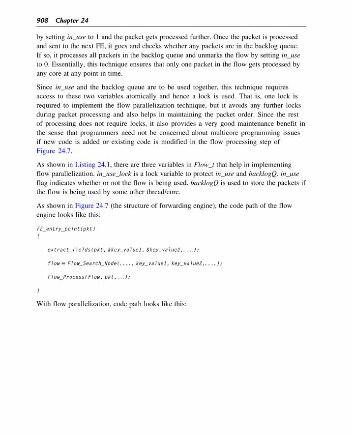
As shown in Figure 24.7 (the structure of forwarding engine), the code path of the flow

engine looks like this:

FE_entry_point(pkt){

extract_fields(pkt, &key_value1, &key_value2,. . ..);

flow 5 Flow_Search_Node(. . .., key_value1, key_value2,. . ..);

Flow_Process(flow, pkt, . . .);

}

With flow parallelization, code path looks like this:

908 Chapter 24

Listing 24.6:

FE1.


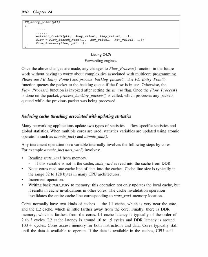
Listing 24.7:

Forwarding engines.

Once the above changes are made, any changes to Flow_Process() function in the future

work without having to worry about complexities associated with multicore programming.

Please see FE_Entry_Point() and process_backlog_packes(). The FE_Entry_Point()

function queues the packet to the backlog queue if the flow is in use. Otherwise, the

Flow_Process() function is invoked after setting the in_use flag. Once the Flow_Process()

is done on the packet, process_backlog_packets() is called, which processes any packets

queued while the previous packet was being processed.

Reducing cache thrashing associated with updating statistics

Many networking applications update two types of statistics � flow-specific statistics and

global statistics. When multiple cores are used, statistics variables are updated using atomic

operations such as atomic_inc() and atomic_add().

Any increment operation on a variable internally involves the following steps by cores.

For example atomic_inc(stats_var1) involves:

• Reading stats_var1 from memory.

• If this variable is not in the cache, stats_var1 is read into the cache from DDR.

• Note: cores read one cache line of data into the caches. Cache line size is typically in

the range 32 to 128 bytes in many CPU architectures.

• Increment operation.

• Writing back stats_var1 to memory: this operation not only updates the local cache, but

it results in cache invalidations in other cores. The cache invalidation operation

invalidates the entire cache line corresponding to stats_var1 memory location.

Cores normally have two kinds of caches � the L1 cache, which is very near the core,

and the L2 cache, which is little farther away from the core. Finally, there is DDR

memory, which is farthest from the cores. L1 cache latency is typically of the order of

2 to 3 cycles. L2 cache latency is around 10 to 15 cycles and DDR latency is around

1001 cycles. Cores access memory for both instructions and data. Cores typically stall

until the data is available to operate. If the data is available in the caches, CPU stall

910 Chapter 24

cycles are fewer. Hence, programmers like to ensure that the data is in the cache as

much as possible.

As discussed above, atomic_inc() and atomic_add() operations update the memory with

new values. This results in invalidation of this memory location in other core caches. When

another core tries to do an atomic_inc() operation on the same statistics variable, it goes to

DDR memory as the cache for this memory location is no longer valid in its cache. The

core needs to wait for 1001 cycles for DDR access.

Consider a case where cores are processing packets in round-robin fashion and let us also assume

that the processing of each packet results in stats_var1 getting incremented. Also consider that

there are two cores working on this packet-processing application. Core 1 getting packet 1

increments stats_var1 and this invalidates the core2 cache line having stats_var1. When packet 2

is processed by core 2, it needs to get the stats_var1 from DDR as the stats_var1-related cache

line was invalidated. When core 2 updates stats_var1 with a new value, this results in

invalidation of the core 1 cache line having stats_var1. When packet 3 is processed by core 1,

core 1 needs to go to DDR to fill its cache and the update of statistics variable invalidates the

core 2 cache, and this can go on if packets are being processed alternately by cores. This

effectively masks the cache advantage and hence leads to performance issues.

Programmers can avoid these repeated cache invalidations by ensuring that the flow is

processed by the same core all the time. Though this is possible in some applications, it is

not typically advised to bind flows to cores as it may result in under-utilization of cores.

Moreover this technique only works for flow-based statistics variables at most and can’t be

applied to global statistics.

Per-core statistics is one of the techniques programmers are increasingly using to reduce

cache thrashing issues associated with statistics updates by multiple cores. This technique

defines as many statistics copies as there are cores. Each core updates its copy of statistics

only. Due to this, there is no need for atomic operations on the statistics variables.

Example: consider a module having two global counters that get updated for each packet.

Per CPU statistics are defined as shown below.

structmodStatistics{intCounter1;intCounter2;};structmodStatisticsstatsArray[NR_CPUS];

NR_CPUS: number of cores dedicated to the module. This could be number of threads if

the module is implemented in Linux user space using pthreads.


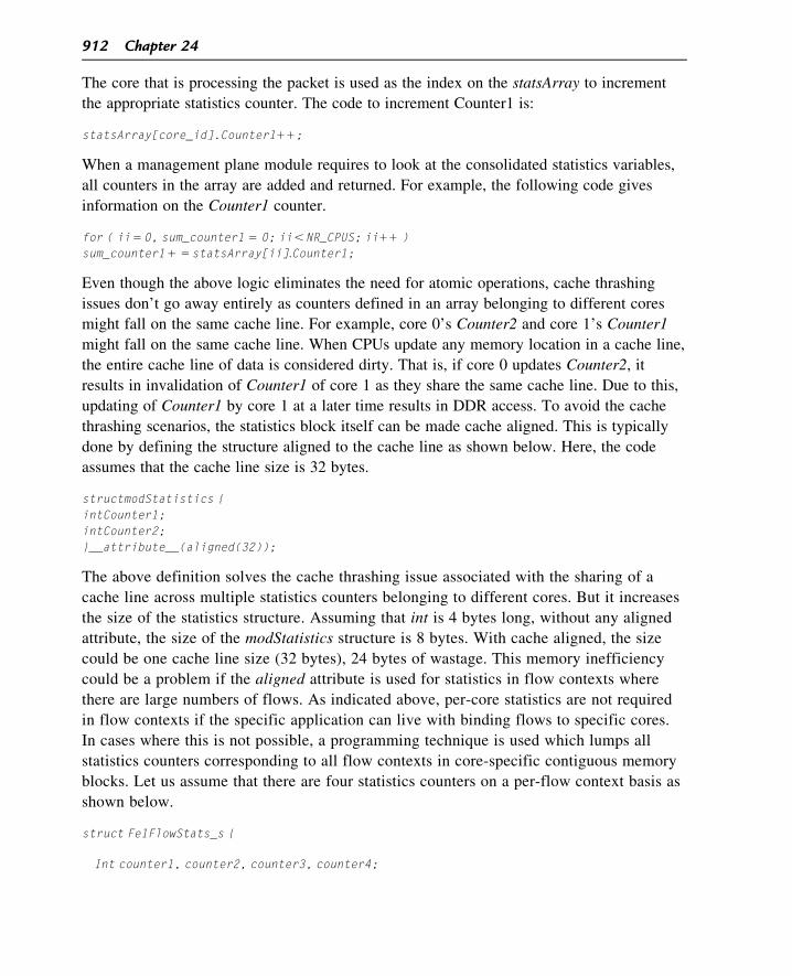
The core that is processing the packet is used as the index on the statsArray to increment

the appropriate statistics counter. The code to increment Counter1 is:

statsArray[core_id].Counter111;

When a management plane module requires to look at the consolidated statistics variables,

all counters in the array are added and returned. For example, the following code gives

information on the Counter1 counter.

for ( ii50, sum_counter1 5 0; ii,NR_CPUS; ii11 )sum_counter11 5statsArray[ii].Counter1;

Even though the above logic eliminates the need for atomic operations, cache thrashing

issues don’t go away entirely as counters defined in an array belonging to different cores

might fall on the same cache line. For example, core 0’s Counter2 and core 1’s Counter1

might fall on the same cache line. When CPUs update any memory location in a cache line,

the entire cache line of data is considered dirty. That is, if core 0 updates Counter2, it

results in invalidation of Counter1 of core 1 as they share the same cache line. Due to this,

updating of Counter1 by core 1 at a later time results in DDR access. To avoid the cache

thrashing scenarios, the statistics block itself can be made cache aligned. This is typically

done by defining the structure aligned to the cache line as shown below. Here, the code

assumes that the cache line size is 32 bytes.

structmodStatistics {intCounter1;intCounter2;}__attribute__(aligned(32));

The above definition solves the cache thrashing issue associated with the sharing of a

cache line across multiple statistics counters belonging to different cores. But it increases

the size of the statistics structure. Assuming that int is 4 bytes long, without any aligned

attribute, the size of the modStatistics structure is 8 bytes. With cache aligned, the size

could be one cache line size (32 bytes), 24 bytes of wastage. This memory inefficiency

could be a problem if the aligned attribute is used for statistics in flow contexts where

there are large numbers of flows. As indicated above, per-core statistics are not required

in flow contexts if the specific application can live with binding flows to specific cores.

In cases where this is not possible, a programming technique is used which lumps all

statistics counters corresponding to all flow contexts in core-specific contiguous memory

blocks. Let us assume that there are four statistics counters on a per-flow context basis as

shown below.

struct Fe1FlowStats_s {

Int counter1, counter2, counter3, counter4;

912 Chapter 24

};Struct Fe1flow_s {struct Fe1FlowStats_s stats;} Fe1Flow_t;

Statistics blocks are referred from the flow context using an array of pointers as shown

below.

struct Fe1flow_s {

struct Fe1FlowStats_s *stats[NR_CPUS];} Fe1Flow_t;

The organization of statistics looks like Figure 24.10 where there are two cores

(NR_CPUS 5 2).

Stats[0]pointer

Stats[1]pointer

Flow Context 1

Stats[0]pointer

Stats[1]pointer

Flow Context N

Stats[0]pointer

Stats[1]pointer

Flow Context 2

Mem

ory assigned to core 0

Stats block 1 (Memory for all four counters)


Stats block N (Memory for all four counters)

Mem

ory Assigned to C

ore 1



Stats block N (Memory for all four counters)

Figure 24.10:Software-based statistics management.


This programming method ensures that core-0-specific counters across flow contexts are

within a contiguous memory block. Similarly core 1 statistics counters across all flow

contexts are in another memory block. These bigger memory blocks are cache aligned. No

cache alignment is required across stats blocks. Any update by counters by core 0 does not

thrash core 1 cache as core 0 and core 1 statistics for any flow are not on the same cache

line and vice versa. But it adds one additional complexity where stats blocks are allocated

as part of flow context creation. This may add to a few more core cycles during flow

context set-up, but cache thrashing on a per-packet basis is avoided. Since there will be a

good number of packets within a flow, this trade-off in flow creation is accepted in many

implementations.

Statistics acceleration

Some multicore SoCs provide a special feature called statistics acceleration. If these

SoCs are used, then there is no need for any of the techniques described above. Only

one copy of statistics counters can be defined in flow contexts. No atomic operation is

required and there are no cache thrashing issues. It simplifies programming quite a bit.

Note that statistics acceleration is not available on many SoCs and hence the above

techniques are still useful where statistics acceleration is not available.

Multicore SoCs supporting statistics acceleration provide special instructions to update

statistics. These instructions increment, add and perform other operations on counters

without involving the cache. Also, multiple cores can fire these instructions at the same

time. Statistics accelerators have the capability to pipeline fired operations and ensure

that all fired operations are executed reliably. Cores do not wait for operation

completion and move on to execute further instructions. This is considered acceptable as

statistics counters are only updated but not checked during the packet-processing path.

In summary, having the statistics acceleration feature in SoCs does not increase memory

requirements, avoids atomic operations, and simplifies coding.

General performance techniques for network application programmers

Use cache effectively

Packet processing performance can benefit significantly if programming is done to take

advantage of core caches effectively. As discussed earlier in this chapter, if cores do not

find data in the caches they go to DDR. The core stalls until the data is available in its

registers, which can be of the order of 100 core cycles. Performance can be improved if

programmers ensure that data is in the caches. Programmers can ensure this by following

some good coding practices. Some of the methods that can be used to take advantage of

caches are described below.

914 Chapter 24

Software-directed prefetching

Many CPU architectures provide a set of instructions to warm its L1 or L2 cache with

cache line worth of data from a given memory location. The Linux operating system, for

example, defines an API function which can be used to prefetch data from DDR into the L1

cache.

char*ptr;ptr 5 ,Pointer to memory location to fetch data from.prefetch(ptr);

Linux and CPU architectures don’t generate an exception even if an invalid pointer is

sent to the prefetch() API built-in function and hence it can be used safely. prefetch()

does actual prefetching in the background, that is, the core does not stall waiting for

data to be placed in the cache and goes on executing further instructions. Hence it can

be used to fetch data that is required at a later time.

In data-plane processing, this technique can be used to fetch the next module flow context

while the packet is being processed in the current module. For example, FE1 in Figure 24.6

can prefetch the FE2 flow context while FE1 is processing the packet. By the time FE2 gets

hold of the packet, the FE2 context would have already been fetched into the L1 cache by

the core subsystem, thereby saving on-demand DDR accesses. Though this may not be

possible in some cases, it is possible in many cases. For example, it is possible to do

prefetching of the FE2 flow context in FE1 if the FE1 flow context is a subset of the FE2

flow context.

The prefetch operation can also be issued in any memory/string library operations. Memory

copy, strcpy, strstr or any operations of this sort can use prefetch of the next cache line of

data while working on current data.

Use likely/unlikely compiler built-ins

Cores having intelligent prediction logic proactively fetch instructions in the memory next

to the instruction that is being executed into the caches. Core usage is more optimal if

instructions that are going to be executed are available in the caches. Conditional logic

(if condition) in the programs is one of the main reasons why the next instruction that gets

executed is not in the caches. Thus, the next instruction fetch results in DDR stalls. By

using likely/unlikely built-in primitives programmers can ensure that most commonly

executed code is together.


Locking critical piece of code in caches

Cache size is often less than the data path code size. Hence cores make space for new code

by removing old code from the cache. CPU architectures provide a facility to lock some

code (memory location and size) permanently in the cache. Programmers can take

advantage of this feature to lock small, commonly executed code in caches. It improves the

performance of data-plane engines. However, this feature in CPU architectures should be

used carefully as the locked portion of the cache is dedicated and hence the overall cache

available for the rest of the code is reduced.

General coding guidelines

Some additional guidelines that help in embedded programming:

• Do not initialize function local variables when they are declared. Initialize them only

when required. Based on the code path that is being taken at that time, some local

variables may not be used at all. In those cases, core cycles need not be expended to do

the initializations.

• Define inline and macros for most commonly used operations.

• Avoid buffer copies, string compares, and allocations in the packet-processing path as

much as possible.

• Utilize hardware acceleration features. Some examples are:

• Packet parsing and fields extracted by hardware

• TCP, IPv4 checksum verification on incoming packets and generation on outgoing

packets

• IP reassembly, IP fragmentation, TCP large receive offload, TCP segmentation

offload, etc.

• Quality of service

• Cryptography, compression/decompression, timer, XML, and pattern-matching

offloads.

Linux operating system for embedded network devices

General-purpose operating systems such as Linux are used to implement control and

management planes. A bare-metal executive in a separate partition with dedicated cores is

one popular approach to implementing data-plane engines. As the complexity of data-plane

engines goes up, general-purpose operating systems are preferred by system designers. By

using general operating systems to implement software for all planes, designers have a

choice of dedicating cores as well as sharing cores across multiple software entities.

916 Chapter 24

Since Linux is one of the popular operating systems used in network devices, this section

concentrates on Linux. Linux, like other general-purpose operating systems, has two

execution spaces � kernel and user space. Control and management-plane software are

typically implemented as Linux user-space executables in order to take advantage of the

vast repository of libraries and also the availability of debugging utilities. Since the data

plane and service plane deal with hardware devices, kernel-space programming is used

initially by developers. With the increasing complexity of data-plane engines, Linux user-

space programming is being looked at to implement DP engines too.

There are some concerns in developing DP engines in Linux user space. This section

discusses some of the concerns and how the Linux operating system mitigates those

concerns.

Translation lookaside buffer (TLB) misses associated with user-space programming

Concerns: unlike the Linux kernel, user-space programs use virtual addresses. Virtual

addresses do not have one-to-one correspondence with physical addresses. Cores need to

get hold of physical address from virtual address to read instructions or access data. Cores

use the TLB cache to get hold of physical address from virtual addresses. The TLB is a

cache that the MMU (memory management unit) uses to maintain virtual address to

physical address mappings. Operating systems such as Linux use one TLB entry to map one

page (4 Kbytes worth). The number of TLB entries is limited in multicore SoCs, typically

in the range of a few thousands. Even though program sizes may not be large, the memory

required for millions of flow contexts could be huge. That could result in many TLB misses

while accessing flow context nodes. When the core finds that there is no mapping available

in the TLB for virtual memory while accessing the memory, it generates a fault. The Linux

kernel services this fault and at the end fills up a TLB entry by referring to the page

table associated with user-space processes. Due to this additional processing overhead,

performance can drop if there are many TLB misses.

Solution: the Linux operating system has a facility called huge pages (also called

hugetlbfs). Rather than using 4-K pages, it allows user-space programs to use huge pages of

different sizes. Many CPU architectures including Power cores support huge pages up to

256 Mbytes. Only one TLB entry is required for each huge page. Data-plane engines

supporting millions of flows can be addressed by very few TLB entries. It reduces TLB

misses and in many cases TLB misses reach zero when huge pages are used. The Linux

loader also supports loading of text and data segments on huge pages, thereby reducing the

TLB misses associated with instructions too.

Luckily, multicore SoCs are increasingly providing a feature called hardware page

table walk. This hardware feature walks through the user-space page tables when there is a


TLB miss. Since cores are not involved in servicing TLB misses, performance does not

suffer. If a multicore SoC has this feature, programmers don’t need to do anything to avoid

TLB misses. That is, huge pages are not required when using multicore SoCs with hardware

page table walk support. Multicore SoC vendors provide this support in Linux. Hence DP

developers don’t even need to be aware of this feature.

TLB misses are avoided either by using multicore SoC with hardware page table walk

support or by using huge pages support provided by Linux.

Access to hardware peripherals and hardware accelerators

Concerns: traditional hardware peripherals and accelerators understand only physical

memory addresses. Drivers in the Linux kernel space are used to work with hardware

devices. Accessing hardware devices such as the Ethernet controller and accelerators

through the kernel from user space involves multiple context switches and buffer copies.

Solution: Linux provides memory mapping functionality, whereby hardware device registers

can be mapped directly to user space. Data-plane engines in user-space processes can

access hardware devices without any kernel intervention. Using memory map functionality

(mmap), even physical memory space can be mapped into user space. User-space processes

can program physical addresses for packet buffers in the hardware devices and access the

mapped addresses in user space, thereby avoiding any copies from virtual address buffers to

physical addresses.

Multicore SoCs provide a feature called IOMMU (IO memory management unit) whereby

hardware devices have intelligence to convert virtual memory addresses to physical

addresses before accessing any data from memory. The IOMMU hardware block has

intelligence to look at the page tables to determine the physical addresses from the

programmed virtual addresses. User-space programs using these multicore SoCs don’t even

need to worry about memory mapping of registers or physical memory and yet access

hardware devices and accelerators directly using virtual addresses.

Linux UIO (user-space IO) functionality allows interrupt delivery to user-space programs

via the Linux file IO framework. User-space programs waiting on epoll() or select()

function calls on UIO file descriptors are woken up when the interrupt is generated.

The interrupt delivery mechanism and the ability to access hardware directly from user

space are also helping user-space-based DP implementations.

Deterministic performance

Concerns: bare-metal-based data-plane implementations are run in a separate partition with

dedicated cores. Since the cores are dedicated, there is determinism in performance. Since

918 Chapter 24

Linux is a general-purpose operating system, cores are shared across multiple tasks and

hence the performance determinism can’t be guaranteed.

Solution: pthreads in Linux can be used to create multiple threads in a Linux user-space

process. Each thread can be associated with a core (Linux calls it core affinity). Since it is

one Linux user-space process, the entire virtual address space is shared by all threads,

allowing the run-to-completion programming model even in Linux as in bare-metal

executives. Linux also provides mechanisms to dedicate cores to threads. Once dedicated,

the Linux OS does not schedule these cores to any other user processes or threads. It does

not even execute interrupts on dedicated cores, thereby providing deterministic performance

as achieved in bare-metal executives.

In essence, the Linux operating system advances in using multicore SoCs are paving the

way for developing data-plane engines too in the Linux user space without sacrificing

performance.

Summary

The move to multicore is occurring not only in high-end applications, but even in mid- and

low-end networking applications. Achieving multicore performance is only possible if

software takes advantage of the multiple cores. Multicore programming is not as simple as

single-core programming. A new mindset is required from architecting, designing to coding.

Networking application development in multicore SoCs should not only concentrate on

achieving scalable performance, but also ease development and be maintainable for a long

time. Some of the programming techniques listed in this chapter should help in achieving

this goal. Happy multicore network programming.


software engineering for embedded systems || embedded software for networking applications

Documents