embedded systems and networking approach to …
TRANSCRIPT
EMBEDDED SYSTEMS AND NETWORKING APPROACH TO GUIDANCE AND
ESTIMATION
A Thesis
by
DANIEL GONÇALVES GHAN
Submitted to the Office of Graduate and Professional Studies of
Texas A&M University
in partial fulfillment of the requirements for the degree of
MASTER OF SCIENCE
Chair of Committee, Manoranjan Majji
Committee Members, John E. Hurtado
Daren B. H. Cline
Head of Department, Rodney Bowersox
August 2019
Major Subject: Aerospace Engineering
Copyright 2019 Daniel Ghan

ii
ABSTRACT
Networked embedded systems are valuable tools for guidance and navigation, with
applications ranging from UAV swarms to self-driving cars. LASR Lab is working on projects
that require networked embedded systems running Kalman filters, such as a smart tower that will
send an alert over the Internet if its embedded system detects structural changes in the tower. To
demonstrate the architecture that will support these projects, a demonstration has been made
consisting of a microcomputer and an Inertial Measurement Unit contained in a football-shaped
shell. This football is designed to stream its position and orientation over a network in real time.
Like other LASR Lab projects, the football utilizes a Tinker Board microcomputer and a
VectorNav IMU. Data are streamed in real time to a controller laptop over a Wi-Fi connection
using the Open MPI protocol. An Extended Kalman Filter and an Unscented Kalman Filter for
estimating position, velocity, orientation, and gyroscope biases were developed and implemented
in C++, along with calibration routines for estimating initial conditions and noise parameters. Due
to a lack of reliable measurements and mathematical bugs, the filters were not successful in
estimating position, velocity, or attitude; but the hardware, software, and networking architecture
was demonstrated successfully and can be used in future projects.

iii
ACKNOWLEDGMENTS
Thank you to my advisor, Dr. Majji; and my committee members, Dr. Hurtado and Dr.
Cline, for their guidance and support of this research.
Thank you to Lisa Brown and Dr. White at the Low-Speed Wind Tunnel for allowing me
to use their 3D printer at a reduced cost.
Thank you to all my friends who provided moral support and helped me enjoy my time as
a graduate student. In particular, thank you to Robert, for helping me build the shell of the
demonstration described in this thesis; to Nathan, for being the one friend who showed up to my
defense; and to my girlfriend, Teresa, for being my constant companion and listening to my
frustrations.
Thank you, Mom and Dad, for your love, support, encouragement, and guidance; during
my time as a graduate student and before. Your efforts laid the groundwork for my present and
future success.

iv
CONTRIBUTORS AND FUNDING SOURCES
Contributors
This work was supervised by a thesis committee consisting of Dr. Manoranjan Majji
(advisor) and Dr. John Hurtado of the Department of Aerospace Engineering and Dr. Darren Cline
of the Department of Statistics. Andrew B. Simon designed the demonstration’s power supply. All
other work conducted for the thesis was completed by the student independently.
Funding Sources
Graduate study was supported by a fellowship from Texas A&M University. This work
was also made possible in part by funding from Smart Tower Systems and by sensors provided by
VectorNav Technologies.

v
NOMENCLATURE
DCM Direction Cosine Matrix
EKF Extended Kalman Filter
IMU Inertial Measurement Unit
LASR Lab Land, Air, and Space Robotics Laboratory
MRP Modified Rodrigues Parameter
NED North-East-Down
UAV Unmanned Aerial Vehicle
UKF Unscented Kalman Filter

vi
TABLE OF CONTENTS
Page
ABSTRACT .................................................................................................................................... ii
ACKNOWLEDGMENTS ............................................................................................................. iii
CONTRIBUTORS AND FUNDING SOURCES ......................................................................... iv
NOMENCLATURE ....................................................................................................................... v
TABLE OF CONTENTS ............................................................................................................... vi
LIST OF FIGURES ..................................................................................................................... viii
LIST OF TABLES .......................................................................................................................... x
CHAPTER I INTRODUCTION ..................................................................................................... 1
Motivation ................................................................................................................................... 1
Project Architecture .................................................................................................................... 1 Scope and Structure of Thesis .................................................................................................... 3 Variable Name Conventions ....................................................................................................... 3
CHAPTER II DEMONSTRATION DESIGN ............................................................................... 5
Sensors ........................................................................................................................................ 5
Electrical Power System ............................................................................................................. 5 Physical Layout ........................................................................................................................... 6
Software ...................................................................................................................................... 8
Installing Open MPI on Ubuntu ............................................................................................ 10 Configuring a Controller ....................................................................................................... 12
CHAPTER III KALMAN FILTER THEORY ............................................................................. 14
Kalman Filters ........................................................................................................................... 14 Propagation ........................................................................................................................... 14
Filtering ................................................................................................................................. 15 Extended Kalman Filters .......................................................................................................... 15 Unscented Kalman Filters ......................................................................................................... 16
Propagation ........................................................................................................................... 16 Filtering ................................................................................................................................. 18

vii
CHAPTER IV POSITION AND ATTIDUTE ESTIMATION .................................................... 19
Quaternion Kinematics ............................................................................................................. 19
Sensor Models ........................................................................................................................... 20 Dynamics .................................................................................................................................. 22 Derivation of Acceleration Process Noise ................................................................................ 24 Calibration ................................................................................................................................ 26
Attitude Determination ......................................................................................................... 26
Bias Calibration .................................................................................................................... 27 Calibration Before a Throw .................................................................................................. 29
Initial Conditions ...................................................................................................................... 30
Extended Kalman Filter ............................................................................................................ 31 State Vector Definition and Covariance Reduction .............................................................. 31 Propagation ........................................................................................................................... 32 Filtering ................................................................................................................................. 33
Unscented Kalman Filter .......................................................................................................... 35 State Vector Definition ......................................................................................................... 35
Propagation ........................................................................................................................... 36 Filtering ................................................................................................................................. 37
CHAPTER V RESULTS .............................................................................................................. 38
Hardware and Software Performance ....................................................................................... 38
Stationary Test .......................................................................................................................... 39 Pendulum Tests ......................................................................................................................... 43 Vicon Tests ............................................................................................................................... 46
CHAPTER VI CONCLUSIONS .................................................................................................. 54
REFERENCES ............................................................................................................................. 56

viii
LIST OF FIGURES
Page
Figure 1: General Architecture ....................................................................................................... 2
Figure 2: Demonstration Architecture ............................................................................................ 2
Figure 3: Electrical Power Diagram ............................................................................................... 5
Figure 4: Top Piece of Shell ........................................................................................................... 6
Figure 5: Bottom Piece of Shell ...................................................................................................... 7
Figure 6: Bottom View of Football ................................................................................................. 7
Figure 7: Component Layout .......................................................................................................... 8
Figure 8: Software Flowchart ....................................................................................................... 10
Figure 9: Two-State UKF Propagation ......................................................................................... 17
Figure 10: Bias Calibration ........................................................................................................... 28
Figure 11: EKF Attitude Drift....................................................................................................... 39
Figure 12: UKF Attitude Drift ...................................................................................................... 40
Figure 13: Position Drift ............................................................................................................... 41
Figure 14: Velocity Drift .............................................................................................................. 41
Figure 15: Stationary Test Uncertainties ...................................................................................... 42
Figure 16: Pendulum Test #1 ........................................................................................................ 44
Figure 17: Pendulum Test #2 ........................................................................................................ 44
Figure 18: Pendulum Test Uncertainties....................................................................................... 45
Figure 19: Throw 1 Acceleration .................................................................................................. 46
Figure 20: Throw 1 Estimated Trajectories .................................................................................. 47
Figure 21: Throw 1 Vicon Trajectory ........................................................................................... 47
Figure 22: Throw 1 Uncertainties ................................................................................................. 48

ix
Figure 23: Throw 2 Acceleration .................................................................................................. 48
Figure 24: Throw 2 Estimated Trajectories .................................................................................. 49
Figure 25: Throw 2 Vicon Trajectory ........................................................................................... 49
Figure 26: Throw 2 Uncertainties ................................................................................................. 50
Figure 27: Throw 3 Acceleration .................................................................................................. 50
Figure 28: Throw 3 Estimated Trajectories .................................................................................. 51
Figure 29: Throw 3 Vicon Trajectory ........................................................................................... 51
Figure 30: Throw 3 Uncertainties ................................................................................................. 52

x
LIST OF TABLES
Page
Table 1: Common Variable Modifiers ............................................................................................ 4
1
CHAPTER I
INTRODUCTION
This thesis describes the development and testing of a networked embedded system used
for attitude and position estimation.
Motivation
The immediate motivation for this project was to develop a networked embedded system
and Kalman filters for the Land, Air, and Space Robotics (LASR) Laboratory, a research lab at
Texas A&M that primarily focusses on guidance and estimation for aerospace systems. LASR Lab
is using this architecture to develop a smart tower, and may use similar architecture in future
projects. The smart tower is a radio or cell-phone tower in which an embedded system will use a
Kalman filter to determine if the structural properties of the tower have changed, and if so to send
an alert. Networked embedded systems for estimation and navigation have many potential
applications, including Unmanned Aerial Vehicle (UAV) swarms, [1] self-driving cars, [2] and
even docking spacecraft.
Project Architecture
A vehicle or a smart tower equipped with networked embedded systems will have the
architecture shown in Figure 1. The vehicle or tower contains a microcomputer connected to some
sensors. Software on the microcomputer uses sensor data to estimate some states—in the case of
the smart tower, the natural frequency and damping ratio of the tower—and communicates
wirelessly with other devices.
The demonstration’s architecture, shown in Figure 2, is analogous to the smart tower
architecture. The sensor is a VectorNav VN-100, an IMU that provides acceleration, magnetic
field, and angular velocity measurements; and the microcomputer is a Tinker Board. These are

2
enclosed in a 3D-printed football-shaped shell. The Tinker Board uses Kalman filters to estimate
the football's position, velocity, and orientation. A Wi-Fi router passes these data from the Tinker
Board to a laptop and commands from the laptop to the Tinker Board. These messages are handled
by the Open MPI software library.
Figure 1: General Architecture
Figure 2: Demonstration Architecture
Vehicle or Tower
Microcomputer with Kalman
filter
Sensor
Sensor
Sensor
Router or other networking
device
Other vehicle
Other vehicle
Other vehicle
Wired connection
Wireless connection
Football
Tinker Board with Kalman
filters VN-100
Wi-Fi router and Open MPI
Laptop
Wired connection
Wireless connection

3
Scope and Structure of Thesis
In this thesis, the word “chapter” refers to a numbered chapter (e.g. “Introduction”).
“Section” refers to a first-level division of a chapter (e.g. “Scope and Structure of Thesis”) and
“subsection” refers to a second-level division (e.g. “Installing Open MPI on Ubuntu”). This section
provides an overview of structure and contents of the following chapters in this thesis, which
explain how the football was made, how it was tested, and how it performed.
Chapter II, Demonstration Design, contains detailed descriptions of the football’s hard
components, the demonstration’s software, and how everything was put together.
Chapter III, Kalman Filter Theory, explains what a Kalman filter is and provides the
algorithms of the two Kalman filters developed for the demonstration.
Chapter IV, Position and Attitude Estimation, develops sensor models, dynamic models,
and noise models and converts them into a form that can be used by the Kalman filters. It also
details the calibration routines and initial conditions used by the demonstration.
Chapter V, Results, details the performance of the demonstration architecture, then
describes the tests used to evaluate the Kalman filters’ and the results of those tests.
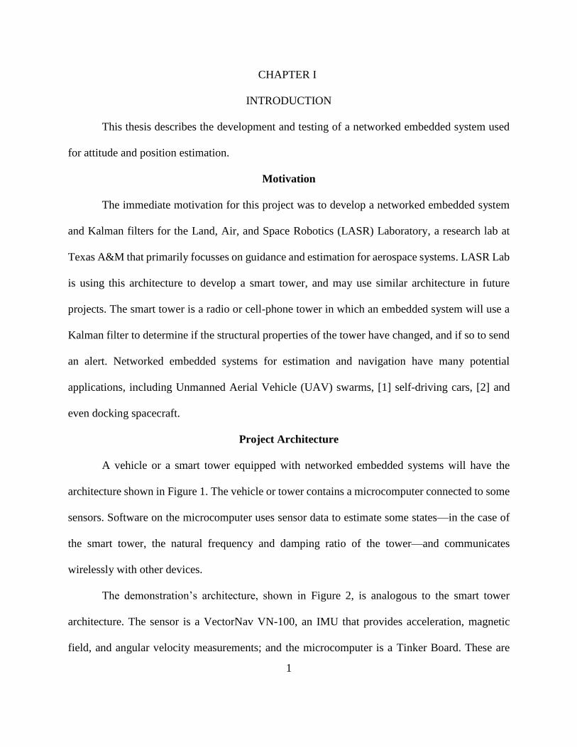
Variable Name Conventions
Some quantities in this thesis have several different variations. For example, there is a true
acceleration, a measured acceleration, and an estimated acceleration associated with each timestep.
Related quantities are denoted by the same letter and are distinguished from each other by various
modifiers. Table 1 lists the common modifiers and their meanings.
4
Table 1: Common Variable Modifiers
Modifier Location Example Meaning
Bolded g Vector quantity
^ Accent �̂� Estimated quantity
~ Accent �̃� Measured quantity
(none) Accent a True quantity, without sensor or estimation error (does not
apply to covariances such a P)
(number) Subscript ω1
Vector component: 𝝎 = [
𝜔1
𝜔2
𝜔3
]
k Subscript 𝒖𝑘 Quantity corresponding to the kth timestep
× Subscript a×
Cross product matrix: 𝒂× ≡ [0 −𝑎3 𝑎2
𝑎3 0 −𝑎1
−𝑎2 𝑎1 0]
𝒂×𝒃 = 𝒂 × 𝒃
– Superscript 𝑃𝑘− Quantity before filtering at timestep k (but after
propagating to timestep k)
+ Superscript 𝑃𝑘+ Quantity after filtering at timestep k (but before
propagating to timestep k + 1)
T Superscript 𝐻𝑘T Matrix transpose
d Before dq True value minus expected value: d𝒒 ≡ 𝒒 − �̂�

5
CHAPTER II
DEMONSTRATION DESIGN
Sensors
The football is designed to estimate its position, velocity, and orientation using
acceleration, angular velocity, and magnetic field measurements. These measurements are
provided by a VectorNav VN-100 IMU. The VN-100 has a 3-axis magnetometer, accelerometer,
and gyroscope and includes its own filters for estimating position, velocity, and orientation. [3]
However, the football makes use only of the uncompensated magnetic, acceleration, angular
velocity, and GPS position; because one purpose of the demonstration is to test the Kalman filters
developed in this thesis, which should not rely on VectorNav’s filtering.
Electrical Power System
The Tinker Board and the VN-100 use electrical power. The VN-100 is powered through
its USB connection to the Tinker Board, and the Tinker Board is powered by a battery. A DC
transformer steps down the voltage from the battery’s 12.6V to the Tinker Board’s 5V, and a 1.5A
fuse protects the Tinker Board from excessive current. Figure 3 is a diagram of this setup.
Figure 3: Electrical Power Diagram
The battery has a switch and two cables—one for charging and one for power output. To
turn on the football, the switch must be in the on position and the Tinker Board connected to the
battery. To charge the battery, the switch must be in the on position, the Tinker Board must be
powered off or disconnected from the battery (the Tinker Board draws more power than the charger
5V 12.6V Battery Fuse DC
transformer
Tinker Board

6
provides), and the battery must be connected to the charger. If the battery is not powering the
Tinker Board or being charged, the switch should be in the off position.
Physical Layout
The football shell is two 3D-printed pieces. Four tabs in the top piece (Figure 4) fit into
slots in the bottom piece (Figure 5) and the two are held together by four #8 screws, one going
through each tab. The screws are held in place by threaded inserts hammered into the sides of the
bottom piece (Figure 6).
Figure 4: Top Piece of Shell

7
Figure 5: Bottom Piece of Shell
Figure 6: Bottom View of Football
All the components inside the shell are fastened to a plywood board that was laser-cut to
fit between a ledge around the rim of the bottom piece (Figure 5) and ledges on the tabs of the top

8
piece (Figure 4). The Tinker Board is fastened to the board by four #4 screws threaded into inserts
mounted on the bottom side of the board. The battery, the transformer, and the VN-100 are attached
using a snap-together fastener similar to Velcro. Figure 7 shows the layout of these components.
Figure 7: Component Layout
Software
The Tinker Board runs Ubuntu, a popular Linux distribution, and has Open MPI installed.
The controller used for the experiments in this thesis was a Dell Inspiron laptop also running
Ubuntu. The subsections at the end of this section contain instructions for installing Open MPI and
setting up a controller. The router used for these experiments was configured to assign static IP
addresses; the Tinker Board was always given the address 10.0.0.20. The football and the
controller do not have to be connected to the same router, as long as there is a path between them
and the football’s IP address is known. The demonstration was successfully tested over an Internet
connection.
The demonstration software is written in C++ and utilizes three non-standard libraries: the
Open MPI library [4] for communications, the VectorNav library [5] for reading sensor data, and
Battery
VN-100
Fuse
Tinker Board
Battery
charging
cable
DC transformer

9
a library called Eigen [6] for linear algebra. An Extended Kalman Filter (EKF) and an Unscented
Kalman Filter (UKF) were written as classes in a header file. One program, called
FootballProgram, resides on the Tinker Board; and another, called FootballReceiver, is on the
controller. Most of the computing is done by FootballProgram; FootballReceiver simply logs and
prints data.
To start the demonstration, the user connects the controller to the router and then runs the
following two commands in the command line (or runs a shell script containing these commands):
ssh 10.0.0.20 "stty -F /dev/ttyUSB0 115200"
which sets the baud rate of communication between the VN-100 to the Tinker Board, and
mpirun --host 10.0.0.20 /home/tinker/Documents/Football/
FootballProgram : --host localhost /home/daniel/Football/
FootballReceiver
which runs the programs. It is important that the Tinker Board’s process is listed first so that it has
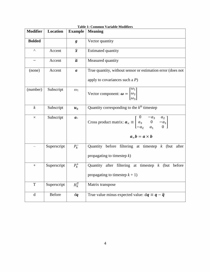
access to user input. The program then proceeds as shown in Figure 8.
10
Figure 8: Software Flowchart
Installing Open MPI on Ubuntu
A Tinker Board can be used like a desktop computer if attached to a monitor, keyboard,
and mouse. The following steps were used to install Open MPI on both the football’s Tinker Board
and the laptop used as the controller.
Pre-throw calibration—estimate sensor noise, gyroscope bias,
and initial attitude
Connect to VN-100
Set initial conditions of EKF and UKF
Wait for measurement or key press
Update EKF
Update UKF
Send states and covariances to
controller
Send “end file” message to controller
Main Menu
Bias Calibration (see Figure 10)
Send “end program” message to controller
End
Run shell script to start program
Log states and covariances
Experiment
Exit Bias Calibration
Start new log file
Measurement
Key press
Close log file
Legend
Controller
Tinker Board

11
1. Connect to the Internet
This is required for Steps 2 and 3. It should be straightforward, but experience has shown that the
Tinker Board’s clock might need to be corrected before connecting (whenever the Tinker Board is
powered off, its clock resets to January 2018).
2. Download Open MPI
Version 4.0.0 was used for the demonstration, but as of the time of writing another version (4.0.1)
has been released. This should not make any difference, but the latest version can be found at
https://www.open-mpi.org/software/ompi/ . Version 4.0.1 can be downloaded by running the
following command:
wget https://www.open-mpi.org/software/ompi/v4.0/downloads/
openmpi-4.0.1.tar.gz
3. Install prerequisite software
Open MPI requires a C++ compiler (e.g. g++), and “make” and a decompressor are required for
the installation. Experience has shown that Ubuntu itself should be up-to-date to ensure the
installation will be successful. Running the following commands will ensure that these
requirements are met and install any missing software:
sudo apt-get update
sudo apt-get install g++
sudo apt-get install make
sudo apt-get install libibnetdisc-dev
4. Install Open MPI
The following commands will decompress and install Open MPI. Installation will take several
minutes and produce much output. Errors during the configure command are to be expected
and do not mean that the installation is failing.

12
tar -xvf openmpi-4.0.1.tar.gz
cd openmpi-4.0.1
./configure --prefix="/home/$USER/.openmpi"
make
sudo make install
cd ..
5. Set path variables
This step is necessary for Linux to be able to find Open MPI commands. Open the file ~/.bashrc
and add the following two lines to the beginning:
export PATH="$PATH:/home/$USER/.openmpi/bin"
export LD_LIBRARY_PATH="$LD_LIBRARY_PATH:/home/$USER/.openmpi/lib/"
To use Open MPI, it will be necessary to open a new terminal window or to run the above
commands in the terminal.
6. Verify Installation
To verify that Open MPI is installed, enter
mpirun --version
This should return a message containing the version number just installed.
Configuring a Controller
The controller needs to have Open MPI installed and Open MPI needs to be able to access
the Tinker Board without a username or password. The following steps were used to configure the
laptop used as the controller for this thesis.
1. Install Open MPI
Follow the steps in the previous subsection.

13
2. Connect the controller and Tinker Board to the same network and know the Tinker
Board’s IP address
Ideally, the Tinker Board should have a static IP address. The router used for this thesis always
assigns the Tinker Board the address 10.0.0.20. If Tinker Board’s IP address is unknown, it may
be necessary to run ifconfig in the Tinker Board’s terminal. The IP address is listed next to
inet, generally in the second block of output text. Use this IP address instead of 10.0.0.20 in the
following steps.
3. Set username for remote access
This step will allow the controller to access the Tinker Board without specifying a username. If
the Tinker Board’s IP address changes, this step (only) will have to be repeated. Open (or create)
the file ~/.ssh/config on the controller and add the following lines:
Host 10.0.0.20
User tinker
4. Share keys
This step will allow the controller to access to the Tinker Board without a password. Run the
following commands on the controller. The first command will have several options; keep pressing
Enter to use the default settings.
ssh-keygen
ssh-copy-id [email protected]
5. Verify
Run the command
mpirun --host 10.0.0.20 hostname
It should return ELAR-Systems.

14
CHAPTER III
KALMAN FILTER THEORY
This chapter provides an overview of the Kalman filter theory. The first section explains
what a Kalman filter is and how it is applied to linear systems. The second and third sections
explain how Extended Kalman Filters and Unscented Kalman Filters, respectively, use the same
principles but apply them to nonlinear systems. The formulas given in this chapter are not specific
to any system; the values of the matrices defined in this chapter, which are specific to the system,
are derived in Chapter IV.
Kalman Filters
Kalman filters estimate a state vector x and a covariance matrix
𝑃 ≡ 𝐸[(𝒙 − �̂�)(𝒙 − �̂�)T] (1)
At generally regular intervals, the filter receives a measurement vector z and updates the state and
covariance estimates, first by propagating them forward in time and then filtering them with the
measurements. These steps utilize linear dynamic and measurement models, respectively.
Propagation
The dynamics of the system are written in discrete form as
𝒙𝑘+1 = Φ𝒙𝑘 + Γ𝒖𝑘 + Υ𝒘𝑘 (2)
where uk is a disturbance vector and wk is a Gaussian process noise vector. The estimates after
propagation are
�̂�𝑘+1− = Φk�̂�𝑘
+ + Γk𝒖𝑘 (3)
𝑃𝑘+1− = Φ𝑘𝑃𝑘
+Φ𝑘T + Υ𝑘𝑄𝑘Υ𝑘
T (4)
where

15
𝑄𝑘 ≡ 𝐸[𝒘𝑘𝒘𝑘T] (5)
Filtering
The measurements are modelled as a linear function of the state plus some zero-mean
Gaussian white noise:
𝒚𝑘 = 𝐻𝑘𝒙𝑘 + 𝜼𝑦𝑘 (6)
𝐸(𝜼𝑦𝜼𝑦T) = 𝑅 (7)
The Kalman gain is defined as
𝐾𝑘 = 𝑃𝑘−𝐻𝑘
T(𝐻𝑘𝑃𝑘−𝐻𝑘
T + 𝑅)−1
(8)
and the expected measurement is
�̂�𝑘 = 𝐻𝑘�̂�𝑘− (9)
The filtered state and covariance estimates are
�̂�𝑘+ = �̂�𝑘
− + 𝐾𝑘(𝒚𝑘 − �̂�𝑘) (10)
𝑃𝑘+ = (𝐼 − 𝐾𝑘𝐻𝑘)𝑃𝑘
− (11)
Extended Kalman Filters
An EKF is similar to a standard Kalman filter except that the state transition matrix can be
a function of the state and the measurement model can be nonlinear:
𝒚𝑘 = 𝒉(𝒙𝑘) + 𝜼𝑦𝑘 (12)
The measurement sensitivity matrix from Equation (6) is approximated as
𝐻𝑘 =𝜕𝒉(𝒙)
𝜕𝒙|�̂�𝑘
−
(13)

16
Unscented Kalman Filters
A UKF handles nonlinear propagation and measurement models differently from an EKF.
A UKF uses considerably more computing power than an EKF but captures some of the
nonlinearity of the original equations. Despite requiring more computing power, UKFs are viable
on small embedded systems; Fico et al. were able to implement a 20-state UKF on a 10€
microcontroller at 35Hz. [7] The UKF used in the demonstration follows the procedure laid out by
Crassidis and Markley in [8].
Propagation
This version of the UKF uses a trapezoidal approximation for the process noise—half is
added to the covariance before propagation (in Equation (15)) and the other half after propagation
(in Equation (21)). For this purpose it is useful to define the following quantity:
�̅�𝑘 =1
2Υ𝑘𝑄𝑘Υ𝑘
T (14)
Let n be the number of states in the filter (not to be confused with n, the normalized
magnetic measurement). Each timestep, a set of 2n + 1 vectors are generated with a mean of the
state vector and a covariance proportional to the covariance matrix. First, a set of 2n vectors is
computed from the columns of Equation (15):
±√(𝑛 + 𝜆)(𝑃𝑘+ + �̅�𝑘) → 𝝈𝑘(𝑖) (15)
where λ is a pre-determined weighting factor and the square root indicates a matrix such that
√𝑋(√𝑋)T
= 𝑋 (16)
These vectors are added to the state vector to create the sigma points:
17
𝝌𝑘+(0) = �̂�𝑘
+ (17)
𝝌𝑘+(𝑖) = �̂�𝑘
+ + 𝝈𝑘(𝑖) (18)
Each sigma point is propagated the same way as a state vector in a standard Kalman filter:
𝝌𝑘+1− (𝑖) = Φ𝑘𝝌𝑘
+(𝑖) + Γ𝑘𝒖 (19)
The post-propagation state estimate is a weighted average of these propagated sigma points:
𝒙𝑘+1− =
1
𝑛 + 𝜆(𝜆𝝌𝑘+1
− (0) +1
2∑𝝌𝑘+1
− (𝑖)
2𝑛
𝑖=1
) (20)
The post-propagation covariance matrix is calculated using Equation (21):
𝑃𝑘+1− =
1
𝑛 + 𝜆(𝜆(𝝌𝑘+1
− (0) − �̂�𝑘+1− )(𝝌𝑘+1
− (0) − �̂�𝑘+1− )T
+1
2∑(𝝌𝑘+1
− (𝑖) − �̂�𝑘+1− )(𝝌𝑘+1
− (𝑖) − �̂�𝑘+1− )T
2𝑛
𝑖=1
) + �̅�𝑘
(21)
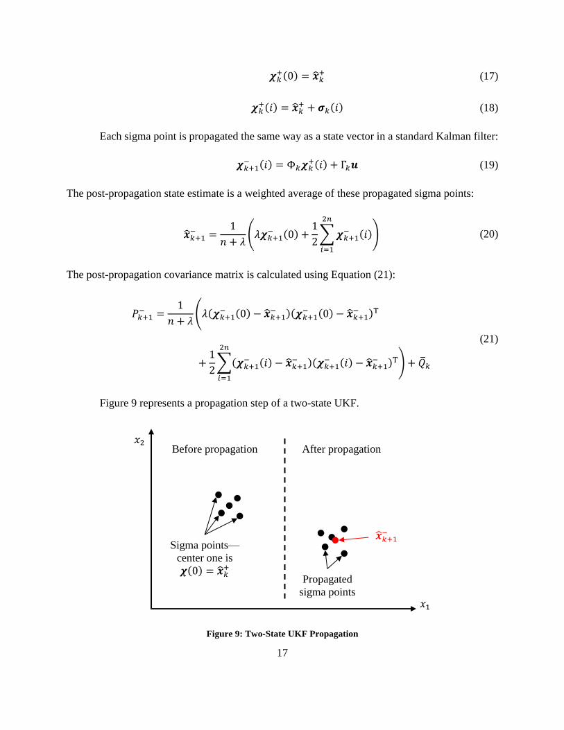
Figure 9 represents a propagation step of a two-state UKF.
Figure 9: Two-State UKF Propagation
𝑥1
𝑥2
Before propagation After propagation
Sigma points—
center one is
𝝌(0) = �̂�𝑘+
Propagated
sigma points
�̂�𝑘+1−

18
Filtering
The UKF has the same measurement model as the EKF (Equation (12)). The expected
measurement is
�̂�𝑘 =1
𝑛 + 𝜆(𝜆𝜸𝑘(0) +
1
2∑𝛾𝑘(𝑖)
2𝑛
𝑖=1
) (22)
where
𝜸𝑘(𝑖) = 𝒉(𝝌𝑘−(𝑖)) (23)
The Kalman gain is calculated using Equation (24); then the state is filtered using Equation (10)
and the covariance using Equation (25).
𝐾𝑘 = 𝑃𝑘𝑥𝑦(𝑃𝑘
𝑣𝑣)−1 (24)
𝑃𝑘+ = 𝑃𝑘
− − 𝐾𝑘𝑃𝑘𝑣𝑣𝐾𝑘
T (25)
where
𝑃𝑘𝑣𝑣 =
1
𝑛 + 𝜆(𝜆(𝜸𝑘(0) − �̂�𝑘 )(𝜸𝑘(0) − �̂�𝑘)
T
+1
2∑(𝜸𝑘(𝑖) − �̂�𝑘)(𝜸𝑘(𝑖) − �̂�𝑘)
T
2𝑛
𝑖=1
) + 𝑅𝑘
(26)
is the innovation covariance and
𝑃𝑘𝑥𝑦
=1
𝑛 + 𝜆(𝜆(𝝌𝑘
−(0) − 𝒙𝑘−)(𝜸𝑘(0) − �̂�𝑘)
T
+1
2∑(𝝌𝑘
−(𝑖) − 𝒙𝑘−)(𝜸𝑘(𝑖) − �̂�𝑘)
T
2𝑛
𝑖=1
)
(27)
is the cross-correlation.

19
CHAPTER IV
POSITION AND ATTIDUTE ESTIMATION
As mentioned previously, the football’s position and attitude are estimated using an EKF
and a UKF. This chapter develops the sensor and dynamic models used for this estimation,
describes the procedures for estimating initial conditions, derives the values of all matrices used
by the filters, and explains how the filters were modified to use quaternions (an
overparameterization) to represent attitude.
Quaternion Kinematics
Quaternion are commonly used to represent rotations. A rotation by an angle α about a unit
axis e is represented as [9]
𝒒 = [
𝑞0
𝑞1
𝑞2
𝑞3
] = [𝑞0
𝑞 ] = [cos
𝛼
2
𝒆 sin𝛼
2
] (28)
(This thesis uses the scalar-first convention.) Because they are more computationally efficient than
direction cosine matrices (DCMs) and, unlike even more efficient methods like Rodrigues
parameters, have no mathematical singularities, the Kalman filters developed for the
demonstration use quaternions to represent attitude. This section provides some quaternion
kinematic equations relevant to the filters.
A quaternion can be converted into a DCM by Equation (29):
𝐶(𝒒) = (2𝑞02 − 1)𝐼3×3 + 2𝑞𝑞T − 2𝑞0𝑞× (29)
The time derivative of the quaternion as a function of the angular velocity vector ω is given by
[10]

20
𝑑𝒒
𝑑𝑡=
1
2Ω(𝝎)𝒒 =
1
2Ξ(𝒒)𝝎 (30)
where
Ω(𝝎) = [
0 −𝜔1 −𝜔2 −𝜔3
𝜔1 0 𝜔3 −𝜔2
𝜔2 −𝜔3 0 𝜔1
𝜔3 𝜔2 −𝜔1 0
] (31)
Ξ(𝒒) = [
−𝑞1 −𝑞2 −𝑞3
𝑞0 −𝑞3 𝑞2
𝑞3 𝑞0 −𝑞1
−𝑞2 𝑞1 𝑞0
] (32)
Sensor Models
Three sensors are used in the demonstration, each with three axes: the accelerometer,
gyroscope, and magnetometer. Each of these sensors assumed to be corrupted by Gaussian white
noise and by biases. The gyroscope bias changes according to the random walk model, but the
accelerometer and magnetometer biases are assumed to be constant. These biases are estimated
during the calibration routines described in the Calibration section.
Mathematically, the gyroscope measurement is modelled as
�̃� = 𝝎 + 𝒃𝜔 + 𝜼𝜔 (33)
Where ω is the true angular velocity, bω is the gyroscope biases and ηω is a Gaussian noise vector
such that
𝑄𝜔 ≡ 𝐸(𝜼𝜔𝜼𝜔T) = [
𝜎𝜔12 0 0
0 𝜎𝜔22 0
0 0 𝜎𝜔32
] (34)
The bias changes according to the random walk model:
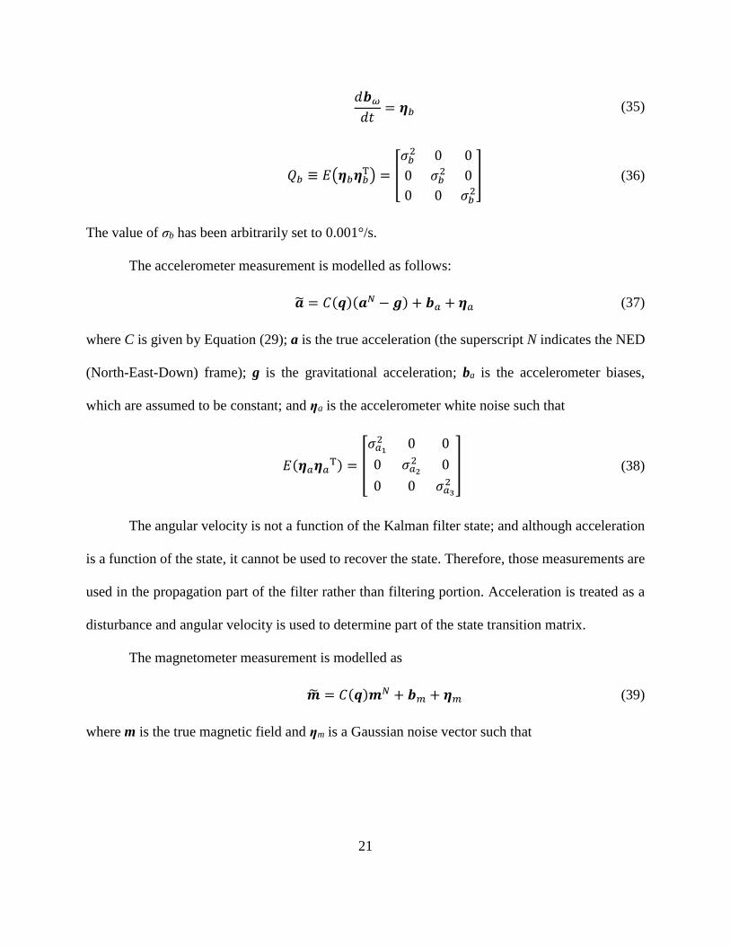
21
𝑑𝒃𝜔
𝑑𝑡= 𝜼𝑏 (35)
𝑄𝑏 ≡ 𝐸(𝜼𝑏𝜼𝑏T) = [
𝜎𝑏2 0 0
0 𝜎𝑏2 0
0 0 𝜎𝑏2
] (36)
The value of σb has been arbitrarily set to 0.001°/s.
The accelerometer measurement is modelled as follows:
�̃� = 𝐶(𝒒)(𝒂𝑁 − 𝒈) + 𝒃𝑎 + 𝜼𝑎 (37)
where C is given by Equation (29); a is the true acceleration (the superscript N indicates the NED
(North-East-Down) frame); g is the gravitational acceleration; ba is the accelerometer biases,
which are assumed to be constant; and ηa is the accelerometer white noise such that
𝐸(𝜼𝑎𝜼𝑎T) = [
𝜎𝑎12 0 0
0 𝜎𝑎22 0
0 0 𝜎𝑎32
] (38)
The angular velocity is not a function of the Kalman filter state; and although acceleration
is a function of the state, it cannot be used to recover the state. Therefore, those measurements are
used in the propagation part of the filter rather than filtering portion. Acceleration is treated as a
disturbance and angular velocity is used to determine part of the state transition matrix.
The magnetometer measurement is modelled as
�̃� = 𝐶(𝒒)𝒎𝑁 + 𝒃𝑚 + 𝜼𝑚 (39)
where m is the true magnetic field and ηm is a Gaussian noise vector such that
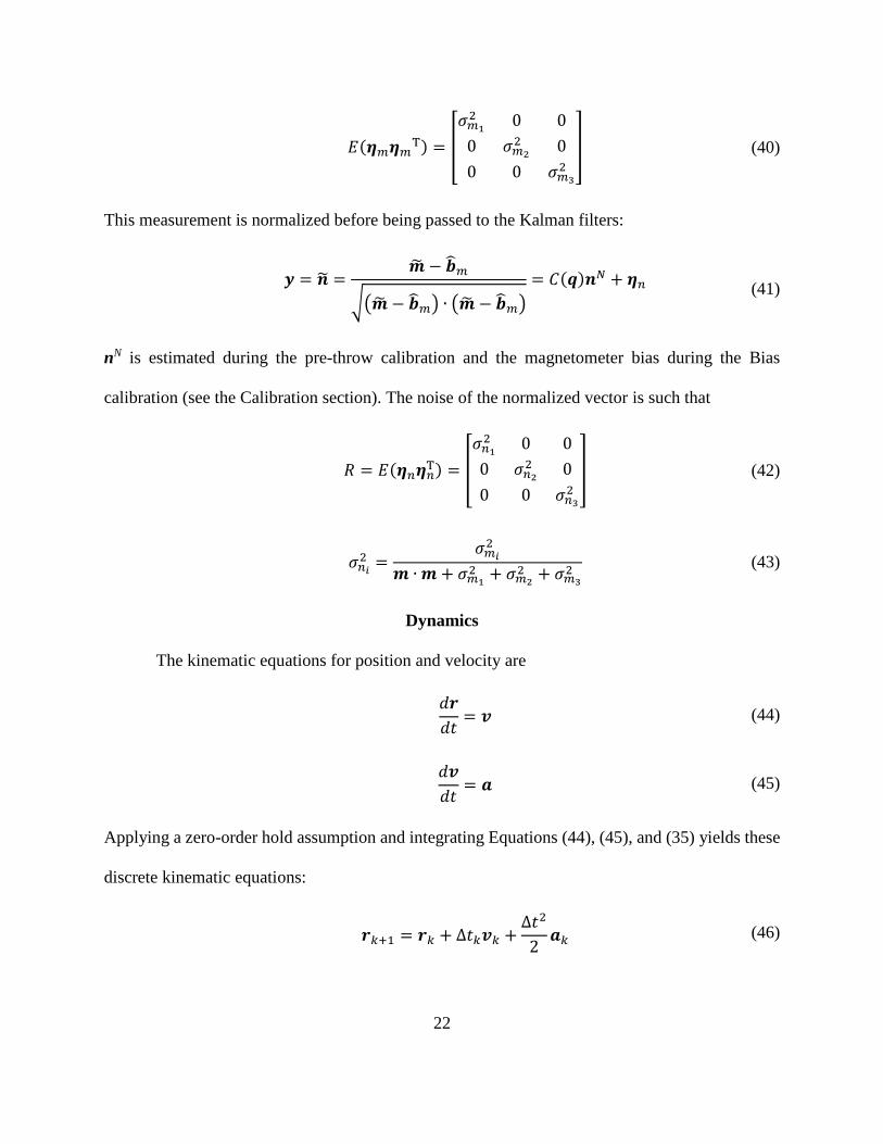
22
𝐸(𝜼𝑚𝜼𝑚T) = [
𝜎𝑚12 0 0
0 𝜎𝑚22 0
0 0 𝜎𝑚32
] (40)
This measurement is normalized before being passed to the Kalman filters:
𝒚 = �̃� =
�̃� − �̂�𝑚
√(�̃� − �̂�𝑚) ∙ (�̃� − �̂�𝑚)
= 𝐶(𝒒)𝒏𝑁 + 𝜼𝑛 (41)
nN is estimated during the pre-throw calibration and the magnetometer bias during the Bias
calibration (see the Calibration section). The noise of the normalized vector is such that
𝑅 = 𝐸(𝜼𝑛𝜼𝑛T) = [
𝜎𝑛12 0 0
0 𝜎𝑛22 0
0 0 𝜎𝑛32
] (42)
𝜎𝑛𝑖
2 =𝜎𝑚𝑖
2
𝒎 ∙ 𝒎 + 𝜎𝑚12 + 𝜎𝑚2
2 + 𝜎𝑚32
(43)
Dynamics
The kinematic equations for position and velocity are
𝑑𝒓
𝑑𝑡= 𝒗 (44)
𝑑𝒗
𝑑𝑡= 𝒂 (45)
Applying a zero-order hold assumption and integrating Equations (44), (45), and (35) yields these
discrete kinematic equations:
𝒓𝑘+1 = 𝒓𝑘 + Δ𝑡𝑘𝒗𝑘 +Δ𝑡2
2𝒂𝑘 (46)
23
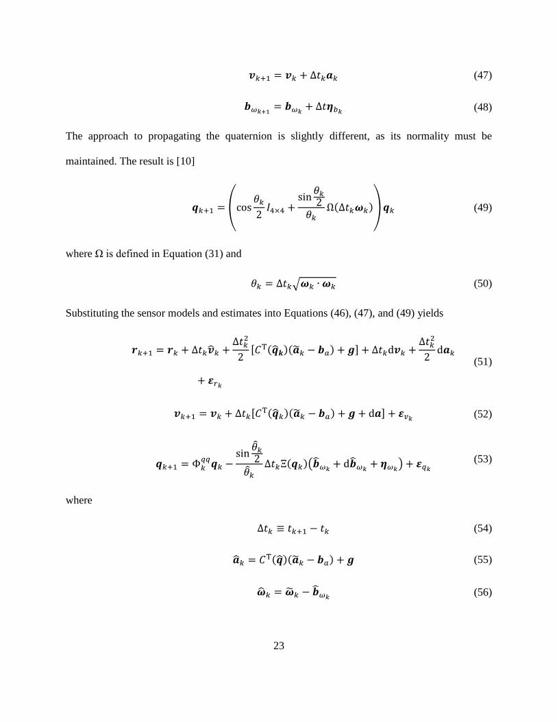
𝒗𝑘+1 = 𝒗𝑘 + Δ𝑡𝑘𝒂𝑘 (47)
𝒃𝜔𝑘+1= 𝒃𝜔𝑘
+ Δ𝑡𝜼𝑏𝑘 (48)
The approach to propagating the quaternion is slightly different, as its normality must be
maintained. The result is [10]
𝒒𝑘+1 = (cos𝜃𝑘
2𝐼4×4 +
sin𝜃𝑘
2𝜃𝑘
Ω(Δ𝑡𝑘𝝎𝑘))𝒒𝑘 (49)
where Ω is defined in Equation (31) and
𝜃𝑘 = Δ𝑡𝑘√𝝎𝑘 ∙ 𝝎𝑘 (50)
Substituting the sensor models and estimates into Equations (46), (47), and (49) yields
𝒓𝑘+1 = 𝒓𝑘 + Δ𝑡𝑘�̂�𝑘 +
Δ𝑡𝑘2
2[𝐶T(�̂�𝒌)(�̃�𝑘 − 𝒃𝑎) + 𝒈] + Δ𝑡𝑘d𝒗𝑘 +
Δ𝑡𝑘2
2d𝒂𝑘
+ 𝜺𝑟𝑘
(51)
𝒗𝑘+1 = 𝒗𝑘 + Δ𝑡𝑘[𝐶T(�̂�𝑘)(�̃�𝑘 − 𝒃𝑎) + 𝒈 + d𝒂] + 𝜺𝑣𝑘
(52)
𝒒𝑘+1 = Φ𝑘𝑞𝑞𝒒𝑘 −
sin𝜃𝑘
2𝜃𝑘
Δ𝑡𝑘Ξ(𝒒𝑘)(�̂�𝜔𝑘+ d�̂�𝜔𝑘
+ 𝜼𝜔𝑘) + 𝜺𝑞𝑘
(53)
where
Δ𝑡𝑘 ≡ 𝑡𝑘+1 − 𝑡𝑘 (54)
�̂�𝑘 = 𝐶T(�̂�)(�̃�𝑘 − 𝒃𝑎) + 𝒈 (55)
�̂�𝑘 = �̃�𝑘 − �̂�𝜔𝑘 (56)

24
Φ𝑘𝑞𝑞 = cos
𝜃𝑘
2I4×4 +
sin𝜃𝑘
2𝜃𝑘
Ω(Δ𝑡𝑘�̃�𝑘) (57)
𝜃𝑘 = Δ𝑡𝑘√�̂�𝑘 ∙ �̂�𝑘 (58)
the d operator is defined in Table 1, and the ε terms represent errors introduced by the zero-order
hold assumption.
Derivation of Acceleration Process Noise
The calculations in this section take place each timestep before propagation, so nearly all
quantities should have the subscript k; and all quaternion quantities should have the superscript +.
For the sake of notational sanity, these subscripts and superscripts have been dropped in this
section.
da is one of the process noise terms in both Kalman filters. This section derives the value
of
𝑄𝑎 ≡ 𝐸(d𝒂d𝒂T) (59)
which is part of the process noise covariance Q, in terms of the quaternion covariance
𝑂 ≡ 𝐸(d𝒒d𝒒T) (60)
which can be obtained from the Kalman filter’s covariance matrix. The convention used in this
section is that the row and column indices of O start at 0, so that
𝑂𝑖𝑗 = 𝐸(d𝑞𝑖d𝑞𝑗) (61)
From Equations (37) and (55),
d𝒂 = [𝐶T(𝒒) − 𝐶T(�̂�)](𝒂 − 𝒃𝑎) + 𝐶T(𝒒)𝜼𝑎 (62)
Substituting Equation (62) into Equation (59),

25
𝑄𝑎 = 𝐸([d𝐶T�̌� + 𝐶T(𝒒)𝜼𝑎][d𝐶T�̌� + 𝐶T(𝒒)𝜼𝑎]T) (63)
where
d𝐶 ≡ 𝐶(𝒒) − 𝐶(�̂�) (64)
�̌� ≡ �̃� − 𝒃𝑎 (65)
Rearranging some terms and recognizing that the sensor noise is uncorrelated to the attitude
estimate,
𝑄𝑎 = 𝐸(d𝐶T�̌��̌�Td𝐶) + 𝐶T(𝒒)𝐸(𝜼𝑎𝜼𝑎T)𝐶(𝒒) (66)
The first expected value in Equation (66) is shown in Equation (68). This was obtained by
linearizing Equation (64) about the estimated attitude, resulting in Equation (67), and substituting
that into the expression.
1
2d𝐶 ≈ 2�̂�0d𝑞0𝐼3×3 + d𝑞�̂�T + �̂�d𝑞T − �̂�0d𝑞× − d𝑞0�̂�× (67)
1
4𝐸(d𝐶T�̌��̌�Td𝐶)
≈ 4�̂�02𝑂0,0�̌��̌�T + (�̂� ∙ �̌�)
2
𝑂1−3,1−3 + �̂��̌�T𝑂1−3,1−3�̌��̂�T
− �̂�02�̌�×𝑂1−3,1−3�̌�× − 𝑂0,0�̂�×�̌��̌�T�̂�× + 𝑋 + 𝑋T
(68)
where
𝑋 = ((𝑂1−3,0 ∙ �̌�) (2�̂�0𝐼3×3 + �̂�×) + ((�̂� ∙ �̌�) 𝐼3×3 − �̂�0�̌�×)𝑂1−3,1−3) �̌��̂�T
+ 2�̂�0 ((�̂� ∙ �̌�) 𝑂1−3,0 − �̌�× (�̂�0𝑂1−3,0 + 𝑂0,0�̂�)) �̌�T
− (�̂� ∙ �̌�) �̂�0�̌�×𝑂1−3,1−3 + (�̂�0�̌�× − (�̂� ∙ �̌�) 𝐼3×3)𝑂1−3,0�̌�T�̂�×
(69)

26
The second expected value in Equation (66) is estimated simply by using the estimated
attitude and the measurement covariance from Equation (38). Thus,
𝑄𝑎 ≈ 4�̂�02𝑂0,0�̌��̌�T + (�̂� ∙ �̌�)
2
𝑂1−3,1−3 + �̂��̌�T𝑂1−3,1−3�̌��̂�T − �̂�02�̌�×𝑂1−3,1−3�̌�×
− 𝑂0,0�̂�×�̌��̌�T�̂�× + 𝑋 + 𝑋T + 𝐶T(�̂�) [
𝜎𝑎12 0 0
0 𝜎𝑎22 0
0 0 𝜎𝑎32
] 𝐶(�̂�)
(70)
Calibration
The demonstration has two calibration routines. This section first describes the attitude
estimation routine used in both calibrations and then the purpose and methods used for each
calibration.
Attitude Determination
Both calibration routines use accelerometer and magnetometer measurements to determine
the football’s orientation in the NED coordinate system. The reference vectors are gravity (which
defines the third axis of the NED frame) and a magnetic field vector based on the World Magnetic
Model (which is used to fix the azimuth but not the elevation). The procedure is shown in
Equations (71) through (78).
cos 𝜃𝑎 = �̂�3 (71)
𝒒𝑎 =
[ cos
𝜃𝑎
2�̂�2
√�̂�12 + �̂�2
2sin
𝜃𝑎
2
−�̂�1
√�̂�12 + �̂�2
2sin
𝜃𝑎
2
0 ]
(72)

27
𝒏𝐼 = 𝒒𝑎 ⊗ �̂� (73)
𝒐𝐼 ≡1
√(𝑛1𝐼 )2 + (𝑛2
𝐼 )2[𝑛1
𝐼
𝑛2𝐼 ] (74)
𝒐𝑁 ≡1
√(𝑛1𝑁)2 + (𝑛2
𝑁)2[𝑛1
𝑁
𝑛2𝑁] (75)
cos 𝜃𝑚 = 𝒐𝐼 ∙ 𝒐𝑁 (76)
𝒒𝑚 =
[ cos
𝜃𝑚
200
± sin𝜃𝑚
2 ]
(77)
𝒒 = 𝒒𝑎∗ ⊗ 𝒒𝑚
∗ (78)
The sign of the ± is the sign of oI × oN, ⊗ represents quaternion multiplication, and the superscript
* represents a quaternion’s conjugate. Half-angle formulas are used to avoid inverse trigonometry.
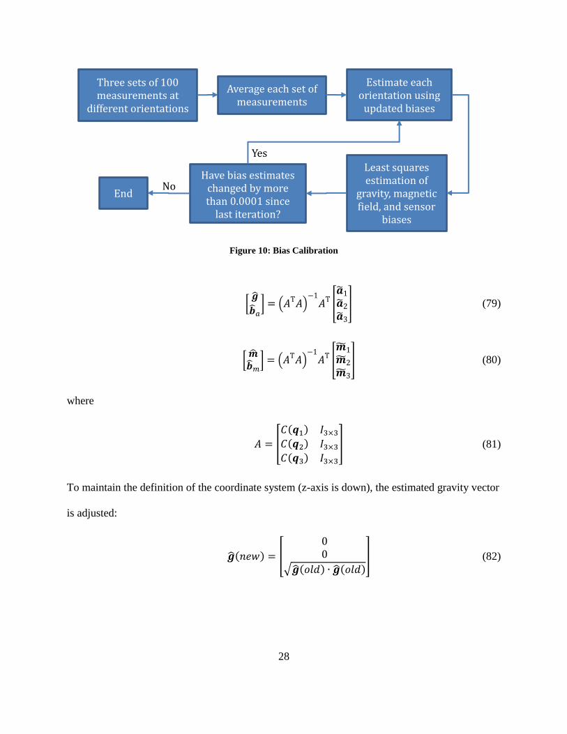
Bias Calibration
The bias calibration estimates the accelerometer and magnetometer biases and the
magnitude of the gravitational acceleration. It is performed automatically after the football is
powered on. The calibration has three stages, with the demonstration asking the user to orient the
football in different ways between stages.
The measurements from each stage are averaged and the algorithm enters a loop, as shown
in Figure 10. Attitude estimation follows the steps laid out in the Attitude Determination
subsection, and the least squares estimation uses Equations (79) and (80).
28
Figure 10: Bias Calibration
[�̂�
�̂�𝑎] = (𝐴T𝐴)
−1𝐴T
[
�̃�1
�̃�2
�̃�3
] (79)
[�̂��̂�𝑚
] = (𝐴T𝐴)−1
𝐴T[
�̃�1
�̃�2
�̃�3
] (80)
where
𝐴 = [
𝐶(𝒒1) 𝐼3×3
𝐶(𝒒2) 𝐼3×3
𝐶(𝒒3) 𝐼3×3
] (81)
To maintain the definition of the coordinate system (z-axis is down), the estimated gravity vector
is adjusted:
�̂�(𝑛𝑒𝑤) = [
00
√�̂�(𝑜𝑙𝑑) ∙ �̂�(𝑜𝑙𝑑)] (82)
Estimate each orientation using
updated biases
Least squares estimation of
gravity, magnetic field, and sensor
biases
Three sets of 100 measurements at
different orientations
Have bias estimates changed by more than 0.0001 since
last iteration?
Yes
No End
Average each set of measurements

29
Calibration Before a Throw
Immediately before each throw, the football must be left stationary for about one second.
100 measurements taken during this period are used to perform the magnetic reference calibration
and estimate the angular rate biases, sensor noise, and initial orientation.
Because the football should be stationary during the calibration, the true angular rates
should be zero and the true acceleration and magnetic field should be constant. The initial angular
rate biases are estimated as the mean of the measured angular rates during the calibration. The
variances in Equations (34), (38), and (40) (of each axis of the gyroscope, accelerometer, and
magnetometer) are estimated using the variances of the measurements taken during the calibration.
The variance of the normalized magnetometer measurements is then calculated using Equation
(43), with the magnetic field estimated during the Bias calibration being substituted for m.
The magnetic reference vector is then updated. By default, its value is
𝒏𝑁 = [0.5071102631985630.0260815272959630.861486468200513
] (83)
which is the World Magnetic Model’s estimate for College Station, Texas (30°35’27”N,
96°21’42”W) normalized. At calibration, this vector is updated so that its elevation matches the
angle between the mean accelerometer and magnetometer measurements (which estimates the
angle between gravity and Earth’s magnetic field). The azimuth is preserved.
𝒏3𝑁(𝑛𝑒𝑤) =
�̃� ∙ �̃�
√(�̃� ∙ �̃�)(�̃� ∙ �̃�)(84)

30
[𝒏1
𝑁
𝒏2𝑁] (𝑛𝑒𝑤) = √
1 − (𝒏3𝑁(𝑛𝑒𝑤))
2
(𝒏1𝑁(𝑜𝑙𝑑))
2+ (𝒏2
𝑁(𝑜𝑙𝑑))2 [
𝒏1𝑁
𝒏2𝑁] (𝑜𝑙𝑑) (85)
Finally, the initial attitude quaternion is estimated as described in the Attitude
Determination subsection.
Initial Conditions
This section gives the initial state and covariance estimates used by the Kalman filters. The
EKF and UKF define the state differently, but both contain the football’s position, velocity,
attitude, and gyroscope biases.
The position is estimated relative to the initial position on any given run. Therefore, by
definition, the initial position and its covariance are zero.
The football is assumed to be stationary at the beginning of the run (the pre-throw
calibration relies on that assumption). Therefore, the initial velocity and its covariance are also
zero.
The initial attitude is estimated during the pre-throw calibration. Its covariance was
arbitrarily set at
𝐸(d𝒒0d𝒒0T) = [
0.000001 0 0 00 0.000001 0 00 0 0.000001 00 0 0 0.000001
] (86)
This was converted to the relevant portion of the covariance matrix by Equation (90) for the EKF
and Equation (118) for the UKF.

31
The initial gyroscope biases are also estimated during the pre-throw calibration. Their
initial covariance is estimated as the covariance of the gyroscope measurements taken during that
calibration.
All other cross-covariances are initially zero.
Extended Kalman Filter
State Vector Definition and Covariance Reduction
The EKF’s state is the position, velocity (both in the NED frame), orientation (quaternion
representing the rotation from the NED coordinate system to the sensor’s coordinate system), and
gyroscope biases, in that order:
𝒙 = [
𝒓𝒗𝒒𝒃𝜔
] (87)
The quaternion poses a problem: due to the quaternion constraint qTq = 1, which differentiates to
qTΔq = 0, the covariance matrix P must be singular. Due to the accumulation of numerical errors,
P is unlikely to remain singular for long. To get around this issue, P is reduced to a 12×12 matrix
(losing one row and one column associated with the quaternion) and propagated and filtered
following the methodology laid out by Lefferts et al. in [10]. The reduced covariance matrix is
�̅� = 𝑆T(�̂�)𝑃𝑆(�̂�) (88)
where
𝑆(𝒒) = [
𝐼6×6 06×3 06×3
04×6 Ξ(𝒒) 04×3
03×6 03×3 𝐼3×3
] (89)
The full covariance matrix can be recovered using Equation (90):

32
𝑃 = 𝑆(�̂�)�̅�𝑆T(�̂�) (90)
The quaternion covariance (defined in Equation (60)) is
𝑂 = Ξ(�̂�)�̅�7−9,7−9ΞT(�̂�) (91)
Propagation
The disturbance is defined as
𝒖𝑘 = �̂�𝑘 (92)
and the process noise as
𝒘𝑘 = [
d𝒗𝑘
d𝒂𝑘
𝜼𝜔𝑘
𝜼𝑏𝑘
] (93)
From Equations (51), (52), (53), and (48), it can be shown that:
Φ =
[ 𝐼3×3 Δ𝑡𝑘𝐼3×3 03×4 03×3
03×3 𝐼3×3 03×4 03×3
04×3 04×3 Φ𝑘𝑞𝑞 −
sin𝜃𝑘
2𝜃𝑘
Δ𝑡Ξ(�̂�𝑘+)
03×3 03×3 03×4 𝐼3×3 ]
(94)
Γ𝑘 = [
Δ𝑡𝑘2
2𝐼3×3
Δ𝑡𝑘𝐼3×3
07×3
] (95)
Υ𝑘 =
[ Δ𝑡𝑘𝐼3×3
Δ𝑡𝑘2
2𝐼3×3 03×3 03×3
03×3 Δ𝑡𝑘𝐼3×3 03×3 03×3
04×3 04×3 −sin
𝜃𝑘
2𝜃𝑘
Δ𝑡𝑘Ξ(�̂�𝑘+) 04×3
03×3 03×3 03×3 Δ𝑡𝑘𝐼3×3]
(96)

33
As the noise of each sensor is assumed to uncorrelated, the process noise covariance is
𝑄𝑘 =
[ 𝑃𝑘4−6,4−6
+ 10−6𝐼3×3 0 0 0
0 𝑄𝑎𝑘+ 10−8𝐼3×3 0 0
0 0 𝑄𝜔 + 10−8𝐼3×3 00 0 0 𝑄𝑏]
(97)
where 𝑃𝑘4−6,4−6 is the portion of the covariance matrix corresponding to velocity (the fourth
through sixth rows of the fourth through sixth columns of P) and Qω, Qb, and Qa are given by
Equations (34), (36), and (59) respectively. The identity matrix terms are an attempt to capture the
noise introduced by the zero-order hold assumption; their values were chosen arbitrarily.
The covariance matrix is propagated using modified versions of the state transition matrix
and the matrix multiplying the process noise:
Φ̅𝑘 =
[ 𝐼3×3 Δ𝑡𝑘𝐼3×3 03×3 03×3
03×3 𝐼3×3 03×3 03×3
03×3 03×3 𝐶(�̂�𝑘+1− )𝐶T(�̂�𝑘
+) −Δ𝑡
2𝐼3×3
03×3 03×3 03×3 𝐼3×3 ]
(98)
Υ̅𝑘 = 𝑆T(�̂�𝑘+)Υ𝑘 =
[ Δ𝑡𝑘𝐼3×3
Δ𝑡𝑘2
2𝐼3×3 03×3 03×3
03×3 Δ𝑡𝑘𝐼3×3 03×3 03×3
03×3 03×3 −sin
𝜃𝑘
2𝜃𝑘
Δ𝑡𝑘𝐼3×3 03×3
03×3 03×3 03×3 𝐼3×3 ]
(99)
�̅�𝑘+1− = Φ̅𝑘�̅�𝑘
+Φ̅𝑘T + Υ̅𝑘𝑄𝑘Υ̅𝑘
T (100)
Filtering
The measurement model is given by Equation (39). Applying Equations (41) and (12),
𝒉(𝒙) = 𝐶(𝒒)𝒏𝑁 (101)
34
so
𝐻𝑘 = [03×6
𝜕𝐶(𝒒)
𝜕𝑞0𝒏𝑁
𝜕𝐶(𝒒)
𝜕𝑞1𝒏𝑁
𝜕𝐶(𝒒)
𝜕𝑞2𝒏𝑁
𝜕𝐶(𝒒)
𝜕𝑞3𝒏𝑁 03×3]
�̂�𝑘−
(102)
𝜕𝐶(𝒒)
𝜕𝑞0= 2𝑞0𝐼3×3 + 2𝑞× (103)
𝜕𝐶(𝒒)
𝜕𝑞1= 2 [
𝑞1 𝑞2 𝑞3
𝑞2 −𝑞1 𝑞0
𝑞3 −𝑞0 −𝑞1
] (104)
𝜕𝐶(𝒒)
𝜕𝑞2= 2 [
−𝑞2 𝑞1 −𝑞0
𝑞1 𝑞2 𝑞3
𝑞0 𝑞3 −𝑞2
] (105)
𝜕𝐶(𝒒)
𝜕𝑞3= 2 [
−𝑞3 𝑞0 𝑞1
−𝑞0 −𝑞3 𝑞2
𝑞1 𝑞2 𝑞3
] (106)
The measurement noise covariance R is given by Equation (42).
After propagating the state and covariance, the filter calculates a modified measurement
sensitivity matrix using Equation (107), then the modified Kalman gain using Equation (108). The
standard Kalman gain is recovered using Equation (109), then the state is filtered using Equation
(10) and the covariance using Equation (110).
�̅�𝑘 = 𝐻𝑘𝑆(�̂�𝑘−) (107)
�̅�𝑘 = �̅�𝑘−�̅�𝑘
T(�̅�𝑘�̅�𝑘−�̅�𝑘
T + 𝑅𝑘)−1
(108)
𝐾𝑘 = 𝑆(�̂�𝑘−)�̅�𝑘 (109)
�̅�𝑘+ = (𝐼9×9 − �̅�𝑘�̅�𝑘)�̅�𝑘
− (110)
35
Unscented Kalman Filter
State Vector Definition
The state vector is defined as
𝒙𝑘 ≡ [
𝒓𝑘
𝒗𝑘
𝛿𝒑𝑘
𝒃𝜔
] (111)
where 𝛿𝒑𝑘 is a Modified Rodrigues Parameter (MRP) representation of the attitude error. The
attitude quaternion itself is a separate variable; after each timestep, the quaternion is updated and
the attitude error reset to zero. The relationship between a set of MRPs and a quaternion is given
by
𝒑 =𝑞
1 + 𝑞0(112)
or, inversely,
𝑞0 =1 − 𝒑 ∙ 𝒑
1 + 𝒑 ∙ 𝒑(113)
𝑞 = (1 + 𝑞0)𝒑 (114)
The MRPs have a singularity when the quaternion represents a rotation of 180°, which is why it is
used to represent an attitude error and not the attitude itself.
The covariance of the quaternion, which is required to calculate Qa, is calculated by
approximating the quaternion error as
d𝒒 ≈ 𝑀Δ𝒑 (115)
where

36
𝑀 ≡𝜕d𝒒
𝜕Δ𝒑|Δ𝑝=03×1
= 2Ξ(�̂�) (116)
Thus, the quaternion covariance is
𝑂 = 𝐸(d𝒒0d𝒒0T) ≈ 4Ξ(�̂�)𝐸(Δ𝒑Δ𝒑T)ΞT(�̂�) (117)
Inversely,
𝑃7−9,7−9 = 𝐸(Δ𝒑Δ𝒑T) =1
4ΞT(�̂�)𝐸(d𝒒0d𝒒0
T)Ξ(�̂�) (118)
Propagation
The lower triangular matrix from the Cholesky decomposition is used as the square root in
Equation (16).
The propagation matrices are:
Φ = [
𝐼3×3 Δ𝑡𝑘𝐼3×3 03×3 03×3
03×3 𝐼3×3 03×3 03×3
03×3 03×3 𝐼3×3 −Δ𝑡𝐼3×3
03×3 03×3 03×3 𝐼3×3
] (119)
Γ𝑘 = [
Δ𝑡𝑘2
2𝐼3×3
Δ𝑡𝑘𝐼3×3
06×3
] (120)
Υ𝑘 =
[ Δ𝑡𝑘𝐼3×3
Δ𝑡𝑘2
2𝐼3×3 03×3 03×3
03×3 Δ𝑡𝑘𝐼3×3 03×3 03×3
03×3 03×3 −Δ𝑡𝑘I3×3 03×3
03×3 03×3 03×3 Δ𝑡𝑘𝐼3×3]
(121)
u, w, and Q are the same as those used in the EKF. They are given by Equations (92), (93), and
(97) respectively.

37
Filtering
The measurement model and the measurement covariance are the same as those used by
the EKF. They are given by Equations (101) and (42), respectively.

38
CHAPTER V
RESULTS
Hardware and Software Performance
Overall, the demonstration works. The physical design of the football is robust, and the
EKF and UKF run in parallel at an update frequency of 100Hz without any problems. The
networking works smoothly; data can be printed to the command line in real time and logged to a
file. There is a bug that sometimes causes an extra character to be inserted at the end of each
message; this is a minor problem that can easily be worked around when post-processing the data,
but one that should be addressed in the future.
There is one issue that impacts the performance of the Kalman filters: the magnetometer
does not provide reliable measurements. This may be because VectorNav sensors correct the
magnetometer measurement based on location, but the VN-100 has no GPS and therefore no way
of knowing its location. In any case, the measurements do not match the model (Equation (39)),
which affects the attitude determination algorithm, the Bias calibration, and attitude filtering in
both Kalman filters. The rest of this section describes the steps that were taken to mitigate the
magnetometer issue.
A new routine was implemented to estimate the accelerometer biases. It assumes that the
VN-100 is stationary and perfectly flat and assumes a gravitational acceleration of 9.793404m/s2,
which was calculated based on the latitude and altitude (82m) of College Station. 100
accelerometer measurements are taken and the biases are estimated as their average plus
9.793404m/s2 in the z-axis.
The magnetometer measurement is the only one used in the filtering phase of the Kalman
filters. Its effect on the filters was eliminated by multiplying the Kalman gains by zero, so the

39
Kalman filters could estimate their position attitude only by propagating the accelerometer and
gyroscope measurements. Without any filtering the covariance can only increase with time.
The attitude determination algorithm was left as it was. The algorithm uses the
accelerometer to determine the elevation and the magnetometer to determine the heading, so the
elevation was considered to be reliable but the heading was not. For this reason, the trajectories in
the Vicon Tests section are plotted in two dimensions (vertical and horizontal) instead of three.
The rest of this chapter evaluates the Kalman filters’ performance based on three tests: one
run during which the football was stationary, two during which it was swung on a pendulum, and
three during which it was thrown.
Stationary Test
One test was performed during which the football was kept stationary. It was expected that
the attitude estimates would drift chaotically over time due to the gyroscope noise but remain close
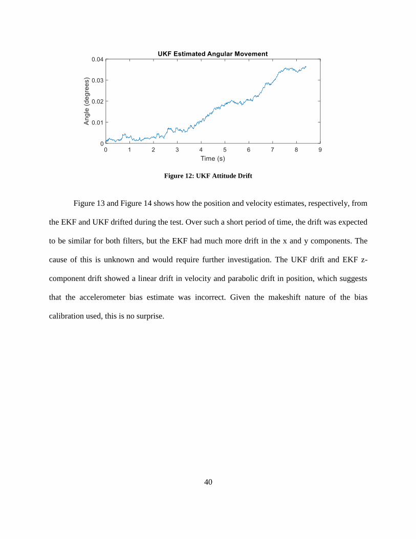
to the original attitude. This was the case for the UKF (Figure 12) but the EKF showed a steady
drift of about 2° per second (Figure 11). Such a constant drift suggests an error in the EKF that has
not been found as of the writing of this thesis, possibly related to the gyroscope bias.
Figure 11: EKF Attitude Drift
40
Figure 12: UKF Attitude Drift
Figure 13 and Figure 14 shows how the position and velocity estimates, respectively, from
the EKF and UKF drifted during the test. Over such a short period of time, the drift was expected
to be similar for both filters, but the EKF had much more drift in the x and y components. The
cause of this is unknown and would require further investigation. The UKF drift and EKF z-
component drift showed a linear drift in velocity and parabolic drift in position, which suggests
that the accelerometer bias estimate was incorrect. Given the makeshift nature of the bias
calibration used, this is no surprise.

41
Figure 13: Position Drift
Figure 14: Velocity Drift

42
Figure 15 shows the uncertainties from the stationary test. The position, velocity, and bias
uncertainties are simply the corresponding diagonal elements of the covariance matrix; the angular
uncertainties are defined as
𝜎𝛼 ≡ √𝐸(d𝛼2) (122)
where α is defined on Page 19. From Equation (28), it can be shown that
𝜎𝛼2 ≈ 𝐸(d𝑞1
2) + 𝐸(d𝑞22) + 𝐸(d𝑞3
2) (123)
These expected values are taken from the quaternion covariance O, which is calculated using
Equation (91) for the EKF and Equation (117) for the UKF.
Figure 15: Stationary Test Uncertainties
×10-3
×10-3
43
As expected, the covariances always increase because the estimates are not being filtered.
The position and velocity uncertainties are much smaller than the actual errors, most likely because
of the error in the accelerometer bias estimates (and the potential bug in the EKF). Without
improving the accelerometer bias estimates, this issue could be fixed by adding terms into the
process noise covariance that take these bias estimation errors into account. A more major issue is
that the UKF has a bug that causes the covariance matrix to drop almost to zero on the first
timestep, as can be seen in the angular and gyroscope bias uncertainties. Despite extensive
searching, this bug has not yet been found as of the time of writing.
Pendulum Tests
Two runs were performed during which the football was swung on a pendulum. The
primary purpose of this test was to evaluate the attitude estimates’ drift when the football is in
motion. Two of the bolts holding the two halves of the football shell together were threaded
through a rope, and the rope was tied to a bar near the ceiling of the LASR Lab. The distance from
the bar to the center of the football was about 377cm. During each test, the football was placed on
a chair to keep it still during the pre-throw calibration and set in motion after the calibration’s
completion.
Accelerometer measurements were used to determine which vector in the football’s
coordinate system pointed down when the pendulum was in its equilibrium state. The pendulum
angle is defined as the angle between this equilibrium down vector and down at any given time.
Even though the rope was free to twist, the pendulum angle is expected to oscillate sinusoidally
with a period of about 3.9s; its local minimum in any given oscillation should be zero. Figure 16
and Figure 17 show the pendulum angles estimated during the two pendulum tests.

44
Figure 16: Pendulum Test #1
Figure 17: Pendulum Test #2

45
The estimated pendulum angles oscillate with approximately the expected period of 3.9s,
but the oscillation is not exactly sinusoidal, especially during the second test. This may be due to
unintended oscillations between the football and the rope; a rigid pendulum with a rigid attachment
to the football would probably solve that problem. The minimum estimated pendulum angle, which
would ideally remain near zero, drifts considerably, especially during the first test. The EKF
performed much worse than the UKF during the first test, possibly because of whatever error
caused the drift in the stationary test.
Figure 18 shows the angular certainties (as defined in Equation (122)) from the pendulum
tests. The uncertainties are much less than the drift observed in the estimated pendulum angles.
One possible cause of this discrepancy is underestimation of the process noise associated with the
zero-order hold assumption.
Figure 18: Pendulum Test Uncertainties
46
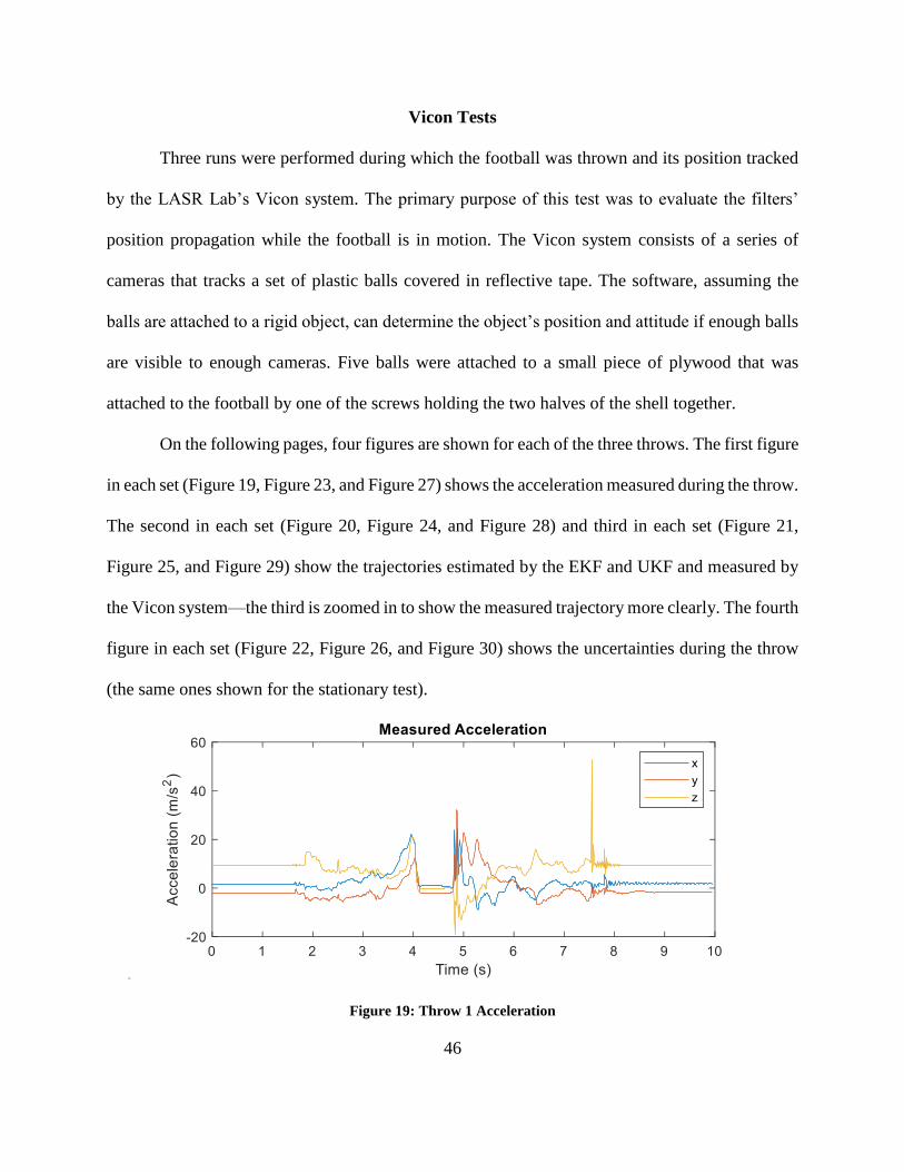
Vicon Tests
Three runs were performed during which the football was thrown and its position tracked
by the LASR Lab’s Vicon system. The primary purpose of this test was to evaluate the filters’
position propagation while the football is in motion. The Vicon system consists of a series of
cameras that tracks a set of plastic balls covered in reflective tape. The software, assuming the
balls are attached to a rigid object, can determine the object’s position and attitude if enough balls
are visible to enough cameras. Five balls were attached to a small piece of plywood that was
attached to the football by one of the screws holding the two halves of the shell together.
On the following pages, four figures are shown for each of the three throws. The first figure
in each set (Figure 19, Figure 23, and Figure 27) shows the acceleration measured during the throw.
The second in each set (Figure 20, Figure 24, and Figure 28) and third in each set (Figure 21,
Figure 25, and Figure 29) show the trajectories estimated by the EKF and UKF and measured by
the Vicon system—the third is zoomed in to show the measured trajectory more clearly. The fourth
figure in each set (Figure 22, Figure 26, and Figure 30) shows the uncertainties during the throw
(the same ones shown for the stationary test).
Figure 19: Throw 1 Acceleration

47
Figure 20: Throw 1 Estimated Trajectories
Figure 21: Throw 1 Vicon Trajectory

48
Figure 22: Throw 1 Uncertainties
Figure 23: Throw 2 Acceleration
×10-3

49
Figure 24: Throw 2 Estimated Trajectories
Figure 25: Throw 2 Vicon Trajectory

50
Figure 26: Throw 2 Uncertainties
Figure 27: Throw 3 Acceleration
×10-3

51
Figure 28: Throw 3 Estimated Trajectories
Figure 29: Throw 3 Vicon Trajectory

52
Figure 30: Throw 3 Uncertainties
The sharp rises in the EKF velocity covariances, which causes the sharp rise in the EKF
position covariances, correspond with sharp spikes in the measured acceleration. This correlation
makes sense because high accelerations increase the acceleration portion of the process noise
covariance, which directly affects the velocity covariance. The UKF should have similar rises in
its covariances; their absence is another sign that something is wrong with the UKF covariance
implementation.
The position estimates degrade so fast that they are absolutely useless after the first few
seconds of motion. The attitude drift observed in the stationary and pendulum tests may explain
×10-3

53
why the position estimate is so bad: when the attitude estimate is not accurate and the football is
not in free fall, the measured acceleration due to the force holding it up does not line up with
gravity, causing the estimated position to fall rapidly. The position and velocity covariances are
much smaller than the errors because, as the stationary and pendulum tests showed, the attitude
error is underestimated.
Throw 1 had a pleasant surprise: unlike in every other run analyzed for this thesis, the
UKF’s covariance did not set itself near zero at the beginning of the run. Without knowing what
causes that issue, it is impossible to say why it did not occur in that run.
54
CHAPTER VI
CONCLUSIONS
The networked embedded system architecture was demonstrated successfully. Other than
a minor issue of extra characters being added to the end of messages, the software and networking
capabilities work without any problems and can be used in future projects or to test new algorithms.
The hardware also works, except that the VN-100’s magnetometer is not reliable. Additionally,
the physical design of the football has two minor shortcomings. Firstly, the battery switch and
cables are only accessible by opening the football. The demonstration would be easier to use if the
battery charging cable and a power switch were accessible through holes in the shell. Secondly,
the cables inside the football, especially the VN-100 cable, are much longer than necessary and
add noticeable weight to the device. This could be remedied by splicing shorter cables and/or
obtaining a custom cable from VectorNav.
The Kalman filters were demonstrated less successfully. In addition to them being
handicapped by the lack of any reliable measurements, multiple bugs are apparent from the tests
performed—one or two that cause the EKF’s attitude and velocity to drift and another that resets
the UKF’s covariance matrix on the first timestep. After a few seconds, both filters’ position and
velocity estimates and the EKF’s attitude estimates are useless. However, other than these
mathematical errors, the Kalman filters work—they do not crash and they were successfully
integrated with the VectorNav software library and Open MPI. Therefore, they provide templates
on which future Extended and Unscented Kalman filters can be built.
The bias calibration routine could not be fully tested because of the magnetometer issue,
but it appeared to work and did not crash. The other calibration routines worked and, like the
Kalman filters, can be used as templates for future calibration routines.

55
Some work would have to be done to be able to demonstrate the Kalman filters
successfully. First, the bugs would have to be found and fixed. Then, the filters would need some
tuning—some of the initial conditions and noise parameters used to generate the data in this thesis
were chosen based on educated guesses rather than any data. Finally, the filters will only be reliable
over a long period of time if they have access to a position measurement and attitude measurements
with at least three degrees of freedom (e.g. two vectors or three angles).

56
REFERENCES
[1] C. Ruiz, X. Chen, L. Zhang, and P. Zhang, "Demo Abstract: Collaborative localization
and navigation in heterogeneous UAV swarms," in 14th ACM Conference on Embedded
Networked Sensor Systems, SenSys 2016, November 14, 2016 - November 16, 2016,
Stanford, CA, United States, 2016: Association for Computing Machinery, Inc, in
Proceedings of the 14th ACM Conference on Embedded Networked Sensor Systems,
SenSys 2016, pp. 324-325, doi: 10.1145/2994551.2996544. [Online]. Available:
http://dx.doi.org/10.1145/2994551.2996544
[2] J. Wang and J. Dang, "Modeling and simulation of traffic characteristics of vehicular ad-
hoc network," Journal of Computational Methods in Sciences and Engineering, vol. 15,
no. 3, pp. 507-513, 2015, doi: 10.3233/JCM-150563.
[3] "VN-100 User Manual." VectorNav Technologies.
https://www.vectornav.com/docs/default-source/documentation/vn-100-
documentation/vn-100-user-manual-(um001).pdf?sfvrsn=b49fe6b9_32 (accessed 16
June, 2019).
[4] "Open MPI: Open Source High Performance Computing." https://www.open-mpi.org/
(accessed 16 June, 2019).
[5] "Downloads." VectorNav Technologies. https://www.vectornav.com/support/downloads
(accessed 16 June, 2019).
[6] B. G. Jacob, Gaël. "Eigen." http://eigen.tuxfamily.org (accessed 16 June, 2019).
[7] V. M. Fico et al., "Implementing the Unscented Kalman Filter on an embedded system:
A lesson learnt," in 2015 IEEE International Conference on Industrial Technology, ICIT

57
2015, March 17, 2015 - March 19, 2015, Seville, Spain, 2015, vol. 2015-June: Institute
of Electrical and Electronics Engineers Inc., in Proceedings of the IEEE International
Conference on Industrial Technology, June ed., pp. 2010-2014, doi:
10.1109/ICIT.2015.7125391. [Online]. Available:
http://dx.doi.org/10.1109/ICIT.2015.7125391
[8] J. L. Crassidis and F. L. Markley, "Unscented filtering for spacecraft attitude estimation,"
Journal of Guidance, Control, and Dynamics, vol. 26, no. 4, pp. 536-542, 2003, doi:
10.2514/2.5102.
[9] J. E. Hurtado, Kinematic and Kinetic Principles. 2016.
[10] E. J. Lefferts, F. L. Markley, and M. D. Shuster, "Kalman Filtering for Spacecraft
Attitude Estimation," Journal of Guidance, Control, and Dynamics, vol. 5, no. 5, pp.
417-429, 1982.