sánchez juny, martí enginyeria civil
TRANSCRIPT

Treball realitzat per:
Flotats Palau, Joan
Dirigit per:
Sánchez Juny, Martí
Grau en:
Enginyeria Civil
Barcelona, 20 de juny de 2016
Departament d’Enginyeria Hidràulica, Marítima i Ambiental
TR
EB
AL
L F
INA
L D
E
GR
AU
2D RIVER FLOOD MODELLING USING HEC-RAS 5.0

ii

iii
2D RIVER FLOOD MODELLING USING HEC-RAS 5.0
Joan Flotats Palau
20/06/2016

iv

v
Abstract
Flooding may occur as an overflow of water from water bodies, such as a river, lake or ocean, in
which the water overtops or breaks levees, resulting in some of that water escaping its usual
boundaries. Floods also occur in rivers when the flow rate exceeds the capacity of the river
channel.
Floods represent the deadliest natural hazard in Europe, resulting in loss of life, damage to buildings,
homes, business and structures such as bridges and roads. Since such consequences are highly
undesirable for human beings, the need to avoid or at least control them has become obvious.
This led to the appearance of hydrodynamic models, numerical tools able to simulate the flow
movement, also in case of flooding. Those models would let us know how the flow behaves in
certain situations and how to act in consequence in order to avoid those undesirable effects.
In April 2016, the new two-dimensional version of HEC-RAS has been released, the so-called
HEC-RAS 5.0. This version is especially interesting since all previous versions of HEC-RAS
had never been able to simulate flows in two dimensions. The main motivation of this document
is to analyse the functionality and workability of HEC-RAS 5.0 regarding two-dimensional
river flooding. In order to do so, three different work approaches have been carried out, with
further analysis of the correspondent results.
First, a detailed intercomparison between the main hydrodynamic models available has been
carried out in order to check the features of the new version of HEC-RAS next to another four
computational programs.
Second, the same case simulation has been performed at the same time for HEC-RAS 5.0 and
for Delft3D. The aim of this is to check the reliability and functionality of HEC-RAS new
version regarding to 2D river flood modelling next to an already developed two-dimensional
model such as Delft3D is. For this simulation, an ideal created prismatic channel has been
chosen in order to work in a basic scenario and two approaches have been analysed: steady non-
flooding and unsteady flooding cases.
Finally, and once its workability has been checked, a more complex case has been simulated
with HEC-RAS 5.0. In this case, the scenario is a real case study, consisting in a river flood in
the Fluvià River, in Catalonia, Spain, with real data of a return period of 50 years, obtained
from Agència Catalana de l’Aigua (ACA) in 2009.
The results led to very sensitive output, realistic and similar to the expected and contrasted.
Thus, one can conclude that, despite small instabilities were found, HEC-RAS 5.0 is able to
perform simple 2D river flood modelling simulations at a similar level of the most advanced
two-dimensional programs, such as Delft3D. However, when it comes to very complex
simulations, some features, such as combination with transport of substances and water quality
or combination with sediment transport and morphological evolution, are not yet available in
two dimensions for HEC-RAS 5.0, so one would rather choose a more advanced model.

vi

vii
TABLE OF CONTENTS
1. INTRODUCTION 1
2. THEORY 3
3. METHODOLOGY 7
4. INTERCOMPARISON OF DIFFERENT HYDRODYNAMIC MODELS 8
4.1. ANALYSIS 8
4.2. RESULTS 16
5. SIMULATION PERFORMANCE 18
5.1. SIMPLE IDEALIZED CASE: PRISMATIC CHANNEL 18
5.1.1. CASE DESCRIPTION 18
5.1.2. CONSIDERATIONS 22
5.1.3. PROBLEMS FOUND 24
5.1.4. RESULTS 25
5.1.4.1. HEC-RAS 5.0 SIMULATION 25
5.1.4.2. DELFT3D SIMULATION 31
5.1.5. EXTRA TESTS: M1 AND M2 CURVES 40
5.2. REAL CASE: FLUVIÀ RIVER 42
5.2.1. CASE DESCRIPTION 42
5.2.2. CONSIDERATIONS 46
5.2.3. PERFORMANCE 47
5.2.4. PROBLEMS FOUND 48
5.2.5. RESULTS 49
5.2.6. CONTRAST WITH IBER 58
5.3. OVERVIEW OF THE SIMULATIONS PERFORMED 60
6. CONCLUSIONS 61
7. REFERENCES 64

viii
LIST OF FIGURES
Figure 1.1. a) Flood in Dutch Rhine, 1996. (Blom, 2015) b) Aerial view of the Danube
Riverin Deggendorf, Germany, June 2013. (Blom, 2015) 1
Figure 2.1. Finite volume discretization for a two-dimensional domain. (Bladé, 2010) 5
Figure 2.2. Different mesh examples in detail, for different applications. (Bladé, 2010) 5
Figure 2.3. Example of RAS Mapper interface 6
Figure 3.1. Methodology followed in this paper 7
Figure 4.1.1. Schematic representation of one-dimensional (X), two-dimensional (X,Y)
andthree-dimensional (X,Y,Z) hydrodynamic models (Cáceres, 2006) 9
Figure 4.1.2. Cross-section example made with HEC-RAS 1D 10
Figure 4.1.3. Example of non-structured mesh composed by triangular elements with
IBER (Bladé, 2010) 11
Figure 4.1.4. Schematic approach of Reynolds-averaged Navier Stoke equations. (Blom,
2015) 12
Figure 4.1.5. a) Afferdense waard during a flood. Mild slope, normal flow is subcritical.
(Blom, 2015); b) Spillway Para dam US. Steep slope, normal flow is supercritical.
(Blom, 2015) 13
Figure 4.1.6. a) Spillway and culvert combination. (The Ras Solution, 2016) b) Bridge
structure.(The Ras Solution, 2016) 14
Figure 4.1.7. a) Confluence between Rio Negro and Amazon River, in Brasil, in which
sediment transport difference between both rivers is noticeable. (Blom, 2015); b)
Amazon River delta, top view. (Blom, 2015) 15
Figure 5.1.1.1. Created channel topography in three-dimensional view, with Delft3D 18
Figure 5.1.1.2. AutoCAD sketch of top and front view of the created channel.
Sketch units in meters (m). Please note the sketch is not on scale. 20
Figure 5.1.1.3. AutoCAD Sketch of longitudinal view of the created channel.
Sketch units in meters (m). Please note the sketch is not on scale. 20
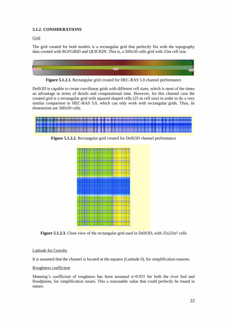
Figure 5.1.2.1. Rectangular grid created for HEC-RAS 5.0 channel performance 22
Figure 5.1.2.2. Rectangular grid created for Delft3D channel performance 22
Figure 5.1.2.3. Close view of the rectangular grid used in Delft3D, with 25x25m2 cells 22
Figure 5.1.2.4. Extension of the downstream end boundary condition for the unsteady
case (left: steady case; right: unsteady case). Example with Delft3D model 23
Figure 5.1.2.5. HEC-RAS Interface with previous default options and chosen options
for the channel 23
Figure 5.1.4.1.1: Channel water depth in steady conditions, with HEC-RAS 5.0 25
ix
Figure 5.1.4.1.2. Location and depth over time graphs for two representative points in
the channel reach, for steady conditions, with HEC-RAS 5.0 25
Figure 5.1.4.1.3. Channel water velocity all over the reach for steady conditions,
with HEC-RAS 5.0 26
Figure 5.1.4.1.4. Location and velocity over time graph for selected point of the ideal
channel, in steady conditions, with HEC-RAS 5.0 26
Figure 5.1.4.1.5. Flooding flow behaviour series of the ideal channel for the unsteady
hydrological data created, with HEC-RAS 5.0 27-28
Figure 5.1.4.1.6. Close view of the area at the downstream end of the reach at
time 21OCT2008 10:45 28
Figure 5.1.4.1.7. Location, water depth over time graph and velocity over time graph of
the two points chosen for analysis in the flooded channel situation, with HEC-RAS 5.0 29
Figure 5.1.4.1.8. Water flow velocity difference between the main channel and the two
floodplains in the flooded channel situation (velocity units in m/s), with HEC-RAS 5.0 30
Figure 5.1.4.2.1. Channel water depth all over the reach in steady conditions, with Delft3D 31
Figure 5.1.4.2.2. Channel water level all over the reach in steady conditions, with Delft3D 31
Figure 5.1.4.2.3. Situation of the three observation points for the steady flow performance
in the channel, with Delft3D 31
Figure 5.1.4.2.4. Graph showing the two water velocity components over time in the
unsteady channel simulation with Delft3D for point (44,28) 32
Figure 5.1.4.2.5. Graph showing the magnitude difference between both velocity
components in the unsteady channel simulation with Delft3D for point (44,28) 32
Figure 5.1.4.2.6. Graph showing the two water velocity components over time in the
unsteady channel simulation for points (224,29) and (408,28) 33
Figure 5.1.4.2.7. Water depth in the channel for steady flow for the three observation
points set 33
Figure 5.1.4.2.8. Graph showing the Froude number all over the reach simulated with
Delft3D for the steady channel situation 33
Figure 5.1.4.2.9. Flooding flow behaviour series of the channel for the unsteady
hydrological data created, with Delft3D 34-35
Figure 5.1.4.2.10. Situation of observation points over the channel reach and floodplains
for unsteady results with Delft3D 36
Figure 5.1.4.2.11. Water depth over time graph of point (224,29) for the flooded channel
situation, with Delft3D 36
Figure 5.1.4.2.12. Water depth over time graph of points (224,43) and (224,12) for the
flooded channel situation, with Delft3D 36
Figure 5.1.4.2.13. Flow velocity general results for unsteady channel case, with Delft3D 37
Figure 5.1.4.2.14. Close view of flow velocity general results for unsteady channel case,
with Delft3D 37
Figure 5.1.4.2.15. Graphs showing the two water velocity components over time and the
relation between them, in the unsteady channel simulation, for point (224,43), with Delft3D 38

x
Figure 5.1.4.2.16. Graphs showing the two water velocity components over time and the
relation between them, in the unsteady channel simulation, for point (224,12), with Delft3D 38
Figure 5.1.4.2.17. Graphs showing the two water velocity components over time and the
relation between them, in the unsteady channel simulation, for point (224,29), with Delft3D 39
Figure 5.1.4.2.18. Graph showing the Froude number all over the reach simulated with
Delft3D for the unsteady channel situation 39
Figure 5.1.5.1. M-type curves (Gutiérrez, 2014) 40
Figure 5.1.5.2.Water depth in the case of M1 curve in the channel. Units in metres. 41
Figure 5.1.5.3. Flow velocity in the case of M2 curve in the channel. Units in metres. 41
Figure 5.1.5.4. Water depth in the case of M2 curve in the channel. Units in metres. 41
Figure 5.1.5.5. Flow velocity in the case of M2 curve in the channel. Units in metres. 41
Figure 5.2.1.1. Fluvià River basin location in Spain (ACA, 2015) 42
Figure 5.2.1.2. Fluvià River reaches and sub basins (ACA, 2015) 43
Figure 5.2.1.3. Domain studied, top view satellite image (Google Maps, 2015) 43
Figure 5.2.1.4. Fluvià hydrograph for T=10 years 45
Figure 5.2.1.5. Fluvià hydrograph for T=50 years 45
Figure 5.2.2.1. a) Thin dam top view (Google Maps, 2015) b) Bridge top view
(Google Maps, 2015) 46
Figure 5.2.3.1. Terrain with the mesh and boundaries applied, with HEC-RAS 5.0 47
Figure 5.2.3.2. Mesh and boundaries used for Fluvià River reach, with HEC-RAS 5.0 47
Figure 5.2.3.3. Detailed view for mesh with squared cells used 48
Figure 5.2.4.1. Flooding flow behaviour series of Fluvià River simulation 1 with
HEC-RAS 5.0 49-50
Figure 5.2.4.2. Non-flooding flow behaviour series of Fluvià River simulation 2,
with HEC-RAS 5.0 51
Figure 5.2.4.3. Flooding flow behaviour series of Fluvià River simulation 3 with
HEC-RAS 5.0 53-54
Figure 5.2.4.4. Maximum water depths at Fluvià River reach in Simulation 3, with
RAS Mapper interface. Units in metres. 55
Figure 5.2.4.5. Maximum flow velocities at Fluvià River reach in Simulation 3 with
RAS Mapper interface. Units in m/s. 55
Figure 5.2.4.6. Location, water depth over time graph and flow velocity over time graph
of two points in the main river channel in Fluvià River Simulation 3, with HEC-RAS 5.0 56
Figure 5.2.4.7. Location, water depth over time graph and flow velocity over time graph
of two points in the northern floodplain in Fluvià River Simulation 3, with HEC-RAS 5.0 57
Figure 5.2.5.1. Maximum depths in Fluvià River simulation obtained with IBER 58
Figure 5.2.5.2. Maximum water elevations in Fluvià River simulation obtained with IBER 59
Figure 5.2.5.3. Figure X: Maximum velocities in Fluvià River simulation obtained with IBER 59

xi
LIST OF TABLES
Table 2.1. HEC-RAS modelling type and analytic tools evolution. (Bladé, 2015) 6
Table 4.2.1. Intercomparison between different hydrodynamic models results table 17
Table 5.1.1.1. Created channel data, set in a simple Excel file 19
Table 5.1.1.2. Hydrological data created for the purpose of the unsteady flow simulation
of the ideal channel 21
Table 5.1.5.1. Boundary conditions set for the M1 and M2 curves in the channel, with
HEC-RAS 5.0 40
Table 5.2.1.1. Hydrograph data for T=10 years (ACA, 2009) 45
Table 5.2.1.2. Hydrograph data for T=50 years (ACA, 2009) 45
Table 5.3.1. Overview table of the simulations performed 60

xii

1
1. INTRODUCTION
Contextualization:
The European Union Floods Directive defines a flood as a covering by water of land not
normally covered by water. Flooding may occur as an overflow of water from water bodies,
such as a river, lake or ocean, in which the water overtops or breaks levees, resulting in some of
that water escaping its usual boundaries. Floods can also occur in rivers when the flow rate
exceeds the capacity of the river channel. (European Comission, 2015)
People have traditionally lived and worked by rivers because the surrounding land is usually flat
and fertile and because rivers provide easy travel and access to commerce and industry. In
consequence, river floods often cause damage to those people, homes and business that are
located in the natural flood plains of rivers, consisting in loss of life, damage to buildings and
other structures such as bridges, roads, sewerage systems or power systems. (Blom, 2015)
There are many examples of floods that occurred in the past. The deadliest flood in the
twentieth century occurred in 1931 in China, in which 70 thousand square miles were flooded
and 3.7 million deaths were estimated. The devastating flood also led to starvation for the next
months, which would also increase the amount of deaths. But not this only flood occurred in
China, five other big floods occurred in the country from 1887 to 1975. However, China is not
the only country that suffered the consequences of flooding. In 2004, Indian Ocean Tsunami led
to 230000 deaths in Indonesia and surrounding countries, such as Thailand and Sri Lanka, and
100000 people were killed in 1971 in North Vietnam due to the Hanoi and Red River Delta
flood. Although the most devastating floods did not happen in Europe, there are also examples
of European deadly floods, such as the so-called St. Felix Flood in The Netherlands, in 1530, in
which more than 100 thousand people were killed, and more recently, the combination of
earthquake, tsunami and fires that happen in Messina in 1908, which ended up killing more than
one hundred thousand people. (O’Connor, 2004)
Not only in the past but also today, floods represent the deadliest natural hazard in Europe.
a b
Figure 1.1. a) Flood in Dutch Rhine, 1996. (Blom, 2015)
b) Aerial view of the Danube River in Deggendorf, Germany, June 2013. (Blom, 2015)
Since such consequences are highly undesirable for human beings, the need to avoid or at least
control them has become obvious. This led to the appearance of hydrodynamic models,
numerical tools able to simulate the flow movement, also in case of flooding. Those models
would let us know how the flow behaves in certain situations and how to act in consequence.
For example, we could figure out that a certain river is especially dangerous in respect to
flooding and we could build a dam in order to control its water flow or, if not possible, could
avoid building next to it or create an efficient warning system.

2
Nowadays, several numerical models are available for flood modelling. Some of them, such as
HEC-RAS, Delft3D, IBER, SOBEK and 3Di, will be explained in detail in the next sections,
but there is a large number of other models that can fulfil the same objectives.
In April 2016, the new two-dimensional (and combined) version of HEC-RAS has been
released, the so-called HEC-RAS 5.0. This version is especially interesting since all previous
versions of HEC-RAS had never been able to simulate flows in two dimensions.
Research question
The initial motivation towards this project is the release of the new version of HEC-RAS,
namely HEC-RAS 5.0, which, as said, introduces for the first time the two-dimensional
approach in this model.
This study aims to analyse the workability, new features and potential of the new version, not
only working with it but also comparing to other models to which it aims to be competitive. The
main focus will be set on flood simulation, since the second case study shows relevant interest
in this aspect.
Two main statements related to the topic are presented:
- First: It is not clear how to choose an appropriate numerical model for flood safety.
- Second: The performance of the new HEC-RAS version is still unknown.
Thus, the main questions that the project aims to answer are the following:
- What are the features of different modelling systems?
- What features are important in order to choose an appropriate model for flooding?
- How does the new HEC-RAS version compare to one of the existing modelling systems?
- To what extent is HEC-RAS 5.0 competitive with other hydrodynamic models, regarding
2D flood modelling?
The first two questions relate to the first statement, while the third and fourth questions relate to
the second statement.
In order to solve the first and second questions, which are definitely related, a detailed analysis
of the main hydrodynamic models is done. The models studied are: HEC-RAS, Delft3D, IBER,
SOBEK and 3Di. A research on which features to analyse in the intercomparison of those
models leads to the answer of the first question. Once the intercomparison between the chosen
features for each of those models is done, a conclusion leads to the answer of the second
question.
Also, the intercomparison results give the keys on how to choose an appropriate model for a
practical comparison with HEC-RAS 5.0. The model chosen for this purpose is Delft3D and the
arguments for this choice are explained in the intercomparison results section.
The third and fourth question have a more practical approach.
For the purpose of the third and fourth questions, this document shows a study of the hydraulic
behaviour of a simple case by means of HEC-RAS 5.0 and Delft3D models, in order to be able
to compare and analyse the results and features of two different models and get to relevant
conclusions.
Besides, once HEC-RAS 5.0 workability is checked next to Delft3D, a real case study is
performed by means of this model. With this more complex and real case study one can check
again the reliability of HEC-RAS 5.0 flood simulations.
Those two cases are first, an idealized prismatic channel reach; and second, a real case based on
a Fluvià river reach, next to Torroella de Fluvià, in Catalonia, Spain. The objective of the latter
is to study the flood extension for hydrological data of a return period of 50 years given by
Agència Catalana de l’Aigua (ACA; Catalan Water Agency) in July 2009.
3
2. THEORY
To be able to understand this document, it is necessary to have a background on the topic. In
this section, it is described what hydrodynamic models are, how they work and their most
relevant properties.
What is, in fact, a hydrodynamic model?
Let us start from the beginning. Hydrodynamics is the study of motion of liquids and, in
particular, the study of motion of water. Thus, a hydrodynamic model is a tool to describe or
represent in some way the motion of water. Although virtually all hydrodynamic models in use
today are computational numerical models, a hydrodynamic model could in fact be a physical
model built on scale, as it was before the advent of widely available computer systems.
Since hydrodynamic modelling is part of the larger field of computational fluid dynamics, those
models used for coastal ocean and river applications have a lot in common with models
developed for meteorology, aerospace and automotive design, ventilation systems, etc. Its
common basis is the numerical solution of the governing equations of conservation of
momentum and mass in fluid. (NOAA, 2015)
How do hydrodynamic models work?
Computational hydrodynamic models are based on a set of equations that describe fluid motion,
the so-called Navier-Stokes equations. Those equations are derived from Newton’s laws of
motion and describe the action of force applied to a fluid; that is, the resulting changes in flow.
This property is called conservation of momentum and is basically Newton’s second law, which
says acceleration is dependent upon the force exerted and proportional to its mass. The
continuity principle is also imposed by computational hydrodynamics. This principle states that
mass and momentum are conserved unless they pass out the domain. In hydrodynamic
modelling, the Navier-Stokes equations are simplified according to the specific characteristics
and properties of the coastal ocean, resulting in the so-called Shallow Water Equations, whose
name expresses the fact that the vertical features are neglected over the horizontal. The Shallow
Water Equations allow for more efficient numerical solution of flow in the oceans, coastal
zones, estuaries, plain rivers and lakes environment, in which the length and width are much
more relevant than the depth.
Rivers, estuaries and oceans are usually very complex systems, which impede an analytical
solution of the governing equations. Computer development has allowed researchers to address
these complex issues through numerical methods. To solve a problem, computers perform
discrete calculations of the continuous governing equations for small individual problems
(breaking the system into multiple small parts) in order to be able to quickly solve the system.
Two classes of approach are commonly used when modelling: structured grid approaches (finite
differences and finite volumes algorithms) and unstructured grid approaches (finite element and
finite volume methods). To form a grid, the domain is separated into numerous components
through a discretization process. Although structured grids provide straightforward and efficient
algorithms, their grid’s flexibility in solving the system is limited since they usually use
quadrilateral cells. Unstructured grid models provide much more flexibility in their grid
resolution by means of employing variable triangular elements. In consequence, they tend to be
more time consuming to run and more sensitive to numerical errors. Both kinds of numerical
methods can be applied to high performance computing systems and are able to simulate
complex coastal and river areas at high resolution.
The accuracy of those models is related to the provided input, this is, the topography and
meteorological conditions. Data such as river inflow and tidal signals at the boundaries are
required in order to run a simulation. (NOAA, 2015)
4
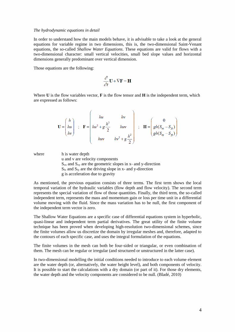
The hydrodynamic equations in detail
In order to understand how the main models behave, it is advisable to take a look at the general
equations for variable regime in two dimensions, this is, the two-dimensional Saint-Venant
equations, the so-called Shallow Water Equations. These equations are valid for flows with a
two-dimensional character: small vertical velocities, small bed slope values and horizontal
dimensions generally predominant over vertical dimension.
Those equations are the following:
Where U is the flow variables vector, F is the flow tensor and H is the independent term, which
are expressed as follows:
where h is water depth
u and v are velocity components
Sox and Soy are the geometric slopes in x- and y-direction
Sfx and Sfy are the driving slope in x- and y-direction
g is acceleration due to gravity
As mentioned, the previous equation consists of three terms. The first term shows the local
temporal variation of the hydraulic variables (flow depth and flow velocity). The second term
represents the special variation of flow of those quantities. Finally, the third term, the so-called
independent term, represents the mass and momentum gain or loss per time unit in a differential
volume moving with the fluid. Since the mass variation has to be null, the first component of
the independent term vector is zero.
The Shallow Water Equations are a specific case of differential equations system in hyperbolic,
quasi-linear and independent term partial derivatives. The great utility of the finite volume
technique has been proved when developing high-resolution two-dimensional schemes, since
the finite volumes allow us discretize the domain by irregular meshes and, therefore, adapted to
the contours of each specific case, and uses the integral formulation of the equations.
The finite volumes in the mesh can both be four-sided or triangular, or even combination of
them. The mesh can be regular or irregular (and structured or unstructured in the latter case).
In two-dimensional modelling the initial conditions needed to introduce to each volume element
are the water depth (or, alternatively, the water height level), and both components of velocity.
It is possible to start the calculations with a dry domain (or part of it). For those dry elements,
the water depth and the velocity components are considered to be null. (Bladé, 2010)

5
Figure 2.1. Finite volume discretization for a two-dimensional domain. (Bladé, 2010)
Figure 2.2. Different mesh examples in detail, for different applications. (Bladé, 2010)
About Delft3D
A brief introduction to Delft3D –and also to its FLOW module– is convenient since it takes
important part in the case study.
Delft3D has been developed by Deltares (Delft, The Netherlands). This fully integrated
software suite provides a multidisciplinary approach and 3D computations for river, coastal and
estuarine zones. Delft3D can simulate flows, sediment transports, waves, water quality,
morphological developments and ecology; and is designed for both experts and non-experts.
Delft3D is a suite composed of several modules that can be executed independently or in
combination with other modules by means of a so-called communication file. Delft3D-FLOW is
one of this modules/components. Delft3D-FLOW is a multidimensional (2D or 3D)
hydrodynamic and transport simulation program that calculates non-steady flow and transport
phenomena that result from tidal and meteorological forcing on a rectilinear or a curvilinear,
boundary fitted grid. In 3D simulations, the vertical grid is defined following the σ co-ordinate
approach. (Deltares, 2014)

6
About HEC-RAS
In this document, HEC-RAS is the model that needs the most attention, since its new version
is its main motivation origin. HEC-RAS has been evolving for the last years and its latest
version –HEC-RAS 5.0.1 version– is capable to simulate the water flow in one and two
dimensions –and also both combined–. The following table shows how HEC-RAS has been
evolving in relation to the different flow conditions:
Table 2.1. HEC-RAS modelling type and analytic tools evolution. (Bladé, 2015)
Version 1D Quasi 2D 2D Permanent
flux
Non-
permanent
flux
Sediment
transport
Water
quality
2.2 ✓ ✓
3.1.3 ✓ ✓ ✓
4.1.0 ✓ ✓ ✓ ✓ ✓ ✓
5.0 ✓ ✓ ✓ ✓ ✓ ✓ ✓
Note: a relevant limitation of HEC-RAS model is that it is not yet capable to apply simulation
of sediment transport and water quality in two dimensions.
HEC-RAS 5.0 uses the equations of Diffusive wave and Saint-Venant by means of the implicit
finite volumes algorithm. The latest version also includes RAS Mapper, an interface window in
which the user integrates the digital model of the land, as an initial step for the flow simulation.
Figure 2.3. Example of RAS Mapper interface
Version 5.0.1 of HEC-RAS includes the following new features (US Army Corps of Engineers,
2016):
1. Two dimensional and combined 1D/2D Unsteady Flow Modelling
2. New HEC-RAS Mapper capabilities and enhancements
3. Automated Manning’s n value calibration for 1D unsteady flow
4. Simplified Physical Breaching algorithm for Dam and Levees
5. Breach Width and development time calculator
6. New hydraulic outlet features for inline structures
7. Sediment transport modelling enhancements: including unsteady flow sediment
transport analyses, reservoir flushing and sluicing, as well as channel stability using
BSTEM integrated within HEC-RAS
8. Completely new 2D User’s Manual
9. Several new example applications within the Applications Guide
10. Updates User’s Manual, Hydraulic Reference Manual, Applications Guide and Help
System

7
3. METHODOLOGY
The study procedure, this is, the numerical modelling will be carried out by means of two
simulation case studies and two different hydrodynamic models: HEC-RAS 5.0 and Delft3D.
Those case studies have only been performed in two dimensions and focusing on the river
flooding simulation approach.
In order to choose which program to compare to HEC-RAS 5.0, a detailed analysis between the
main hydrodynamic models has been first done in the next section. The model finally chosen is,
as mentioned, Delft3D.
The next schematic figure gives an idea of the methodology of this document, from the initial
motivation to the final method.
Figure 3.1. Methodology followed in this paper
HEC-RAS 5.0 release, new version with 2D functionality
Will to know about its workability
How does it compare to other similar 2D models?
Simulate in parallel with a similar and appropriate model in order to be able
to compare
How to choose which is appropriate to compare with
HEC-RAS?
Intercomparison - analysis between 5 main models
ChoiceDelft3D
How does the 2D module work?
Performance of a practical simulation
Next to Delft3D
Ideal case Prismatic channel
In more detail
Real case Fluvià River

8
4. INTERCOMPARISON OF DIFFERENT HYDRODYNAMIC MODELS
4.1. ANALYSIS
For a clear and schematic analysis of the main hydrodynamic modelling systems, one first needs
a detailed explanation of the different features. There are several characteristics to describe
numerical models. However, the most relevant will be discussed in this section.
Dimensions
Hydrodynamic models can be differentiated between one-dimensional (1D), two-dimensional
(2D) and three-dimensional (3D).
On one hand, one-dimensional models are the simplest option. They only need a velocity u and
a water depth d to compute the water flow movement. It is assumed that one of the directions,
the longitudinal direction along the river axis, prevails above the other directions. Thus, these
models are simpler since they do only take into account the longitudinal axis. The hydraulic
data is applied through transversal cross-sections, with average values for each cross-section.
This means that the full cross-section is represented by a single value of velocity, without
consideration of any differential neither horizontally nor vertically. One relevant limitation for
one-dimensional models is that they assume the flow is totally perpendicular to the cross-
section. This kind of models is applicable to very long reaches, generally twenty or more times
larger than the width. (Cáceres, 2006)
One-dimensional models have several advantages, such as:
- They can usually be set up quickly and their computations are fast. Time series
simulations and large networks simulations will generally require only some minutes of
computer time to run
- Can accurately represent cross-sections area of channels at all stages because they do not
require grids to approximate cross-section as two- and three-dimensional models do.
- Little field data is required in order to set up the model
- They generally include more powerful capabilities to describe control structures than two-
and three-dimensional models do
But they also have a main disadvantage, based on the inability to describe two-dimensional
characteristics such as channel meander, circulation within large water bodies or
stratification. (Moffatt and Nichol, 2005)
On the other hand, two-dimensional models are able to describe the movement in two directions
and use both components of velocity (ux, uy) on the horizontal plane. Those models are usually
called shallow water models since they are especially useful for extensive flows (like estuaries
or lakes) where the vertical velocity variation is low. They are not recommended for notable
vertical velocity variations. Those models can be called 2DH models, while 2DV models have
flow velocity components in the vertical plane (one component in the horizontal streamwise
direction and one component in the vertical direction). However, in this document, when one
speaks about two-dimensional models is only referring to 2DH models. 2DV models are not
relevant for the practical part of this document.
A two-dimensional model is indispensable if the problem involves complicated circulation
patterns. However, these models require more data and are more time consuming to run. Also,
two-dimensional have more numerical stability problems. (Moffatt and Nichol, 2005)

9
Finally, three-dimensional models are needed when the vertical component of the velocity (uz)
also takes part. The vertical dimension is modelled though a number of layers which is usually
from two to ten or even more. 3D models represent the most advanced state of modelling. Those
models are capable to calculate the three spatial components of velocity and are therefore
applicable to any practical case, although it might not be recommendable when the horizontal
dimensions are much larger than the vertical dimensions, for practical reasons.
Three-dimensional models provide the most detailed look at a hydrodynamic system, at a
penalty of much longer computer simulation times and the requirement for a substantial amount
of field data to capture the complexities of flow in all three dimensions in the most complex
cases. (Moffatt and Nichol, 2005)
Figure 4.1.1. Schematic representation of one-dimensional (X), two-dimensional (X,Y) and
three-dimensional (X,Y,Z) hydrodynamic models (Cáceres, 2006)
While the old version of HEC-RAS is a one-dimensional model, IBER and SOBEK are two-
dimensional models and, for instance, Delft3D can fulfil the 3D approach.

10
Finite difference and finite element models and grid types
Since water is constituted for a quasi-infinite number of particles, it is very hard to solve the
water flow behaviour of a determined scenario. The way to deal with it is dividing the water
mass in discrete elements with finite size, in order to make management possible for computers.
For the simpler cases of one-dimensional models, such as the previous versions of HEC-RAS,
the discretization is performed through transversal cross-sections. The methodology in this case
consists on balancing the energy in one section and then proceeding with the next one until
finishing all of them. This is a very simple method. Therefore, those programs are generally
robust, fast and reliable.
Figure 4.1.2. Cross-section example made with HEC-RAS 1D
Since two- and three-dimensional cases lead to a differential equation process, a more detailed
discretization through a computational grid is required. This grid has a determined shape and
characteristics that are needed to classify them: structured or unstructured mesh, rectilinear or
curvilinear elements, elements of a determined number of sides (squared, quadtrees…), etc.
The different types of grids are the following (Moffatt and Nichol, 2005):
- Rectangular grids: since real river boundaries have curved shapes, these grids suffer from
the relevant disadvantage that the contour cells do not match a perfect shape and
information is lost (water bodies are represented as stair-step edges). Thus, this requires a
fine grid with small cell sizes.
- Curvilinear orthogonal grids: the curvilinear grid can be fitted along boundaries and
contours. Thus, these grids are able to represent the configuration of a water body more
accurately than rectangular grids do.
- Unstructured grids: sometimes, simulations need to be more detailed somewhere and less
detailed elsewhere. Unstructured grids are appropriate in those cases, because they are
able to incorporate model elements that vary in size. Complex boundaries and contours
can be smoothly fitted. However, they can be very time consuming to set up.
Those grids contain all the elements for which the partial differential equations must be solved.
The two main approaches for this purpose are (Moffatt and Nichol, 2005):
- The finite-difference method: for each time step, represents the water levels at a set of
discrete points. The typical solution grid is a network of straight or curved lines with
nodes at the intersections.
- The finite-element method: the solution domain is divided into a set of triangular or
polygonal elements. The water levels and currents are described as linear or quadratic
functions across each finite element.

11
Generally, finite-difference calculations are more computationally efficient than finite-element
calculations, for a given network size. However, finite-difference models are generally limited
to a rectangular or curved grid, while finite-element grids are more appropriate for irregularly
shaped model domains. In conclusion, finite-difference solutions often require finer grids
with smaller cell sizes than finite-element solutions when modelling complex shapes. Also,
for finite-element solutions, the time step can be longer, which leads to a faster simulation
process. (Moffatt and Nichol, 2005)
One should note that the calculation precision is directly related to the used mesh, and the latter
to the topography quality. Note that this means that if the same case is applied to two different
models with the same cell size and same time step, the level of detail will be exactly the same.
However, the accuracy can be different for different programs.
Figure 4.1.3. Example of non-structured mesh composed by triangular elements
with IBER (Bladé, 2010)

12
Hydrodynamic equations
The hydrodynamic equations used for each model is definitely a main feature to consider. The
equations used can be divided into two main groups: Reynolds-averaged Navier Stokes
equations (RANS) and Horizontal Large-Eddy Simulation equations (HLES).
Figure 4.1.4. Schematic approach of Reynolds-averaged Navier Stoke equations. (Blom, 2015)
Reynolds-averaged Navier Stokes equations (RANS) are the most common used in the main
hydrodynamic models and the ones which are used in this document simulation.
Although the Navier Stokes equations describe the turbulent flux in rivers and that numerical
schemes do exist for its resolution, it is not yet possible to model turbulence flux in an exact
manner. This is due to the fact that for such a small scale, a computational capacity that does not
exist yet would be required. This limitation motivated the development of certain models based
in a statistics approximation in order to model turbulence by means of the so-called Reynolds-
averaged Navier-Stokes equations (RANS). Those equations are obtained from the averaging of
the Navier-Stokes equations in a bigger scale than the turbulence scale. Thus, RANS equations
describe features (velocity, pressure, temperature, et cetera) in average but not the details of the
turbulent fluctuations (Pedrozo-Acuña, 2011).
The Reynolds-averaged Navier-Stokes equations are (Pedrozo-Acuña, 2011):
where ui is the i-component of the velocities vector, ρ is the fluid density, p is the pressure, gi is
the i-component of the acceleration of gravity and τij is the tensor of viscosity tensions
(Pedrozo-Acuña, 2011).
Only Delft3D can work with Horizontal Large-Eddy Simulation equations (HLES), while the
other five cases studied can only perform simulations using Reynolds-averaged Navier Stokes
equations (RANS).

13
Supercritical flow
Sometimes, in a river scenario, one can find that the water depth is higher than the critical water
depth. This state is the so-called slow regime or subcritical flow. Also, one can find the
opposite: a lower water level than the equilibrium. This state is the so-called fast regime or
supercritical flow. Finally, critical flow is the state in which the water depth equals the
equilibrium water depth.
The calculation of the Froude number Fr let us know easily if a river is in supercritical or
subcritical flow state. The Froude number Fr is defined as the division of the inertia forces over
the gravity forces, as follows (Gutiérrez, 2014):
𝐹𝑟 =u
√g · 𝑑𝑒
where u is the flow velocity, g is the acceleration of gravity and de is the equilibrium water
depth.
And, depending on its value, one has:
Subcritical flow if Fr < 1
Critical flow if Fr = 1
Supercritical flow if Fr > 1
a b
Figure 4.1.5. a) Afferdense waard during a flood. Mild slope, normal flow is subcritical. (Blom,
2015); b) Spillway Para dam US. Steep slope, normal flow is supercritical. (Blom, 2015)
Subcritical flow, this is, Froude number Fr < 1, is generally simple and all models are able
to simulate it. However, supercritical flow, this is, Froude number Fr > 1, is particularly
complex for some numerical models, since a rapidly varied flow caused by hydraulic jumps
and crash waves is difficult to model. The most difficult aspect to model is usually the case
in which subcritical and supercritical flow are alternatively switching. For this reason, it is
an important characteristic of models whether they can run supercritical (or combined) flow
or not. (Cáceres, 2006)
In this document, all programs analysed are, to a certain extent, able to model supercritical flow.
14
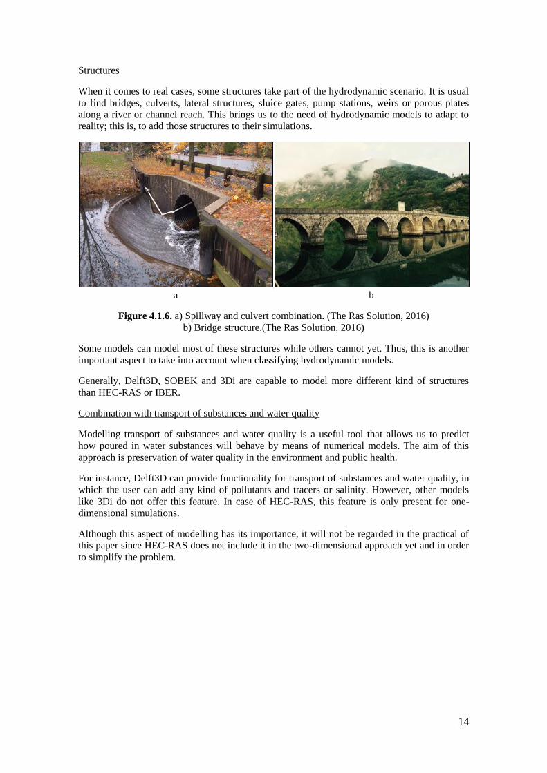
Structures
When it comes to real cases, some structures take part of the hydrodynamic scenario. It is usual
to find bridges, culverts, lateral structures, sluice gates, pump stations, weirs or porous plates
along a river or channel reach. This brings us to the need of hydrodynamic models to adapt to
reality; this is, to add those structures to their simulations.
ab
a a b
Figure 4.1.6. a) Spillway and culvert combination. (The Ras Solution, 2016)
b) Bridge structure.(The Ras Solution, 2016)
Some models can model most of these structures while others cannot yet. Thus, this is another
important aspect to take into account when classifying hydrodynamic models.
Generally, Delft3D, SOBEK and 3Di are capable to model more different kind of structures
than HEC-RAS or IBER.
Combination with transport of substances and water quality
Modelling transport of substances and water quality is a useful tool that allows us to predict
how poured in water substances will behave by means of numerical models. The aim of this
approach is preservation of water quality in the environment and public health.
For instance, Delft3D can provide functionality for transport of substances and water quality, in
which the user can add any kind of pollutants and tracers or salinity. However, other models
like 3Di do not offer this feature. In case of HEC-RAS, this feature is only present for one-
dimensional simulations.
Although this aspect of modelling has its importance, it will not be regarded in the practical of
this paper since HEC-RAS does not include it in the two-dimensional approach yet and in order
to simplify the problem.

15
Combination with sediment transport and morphological evolution
One of the greatest aims of river engineering is the prediction of morphological evolution. In
practical cases, river bed and water flow interact so that bed elevation can change due to the
water flow and vice versa. This feature is important to predict how a bed level will develop in
case of construction of new structures in a river or canal reach such as dams, dikes or bridges,
but also in case of narrowing or widening. (Blom, 2015)
The models offering this feature are the same as the ones that did for the last section. Again,
HEC-RAS can only simulate sediment transport and morphological evolution for one-
dimensional cases and 3Di cannot offer this feature at all.
The same reasons as in combination with transport of substances and water quality bring this
document to leave this feature aside for the practical sections.
a b
Figure 4.1.7. a) Confluence between Rio Negro and Amazon River, in Brasil, in which
sediment transport difference between both rivers is noticeable. (Blom, 2015)
b) Amazon River delta, top view. (Blom, 2015)
Local running availability
Sometimes, the high computational –and economical– costs that a simulation represents are not
affordable for a local –standard– computer. This means that, for some models, certain
equipment is required. For example, local running is possible with models like HEC-RAS,
IBER or Delft3D, but 3Di cannot be ran in a local computer and the purchase of the required
equipment to do so is really expensive –about 20.000€–. (3Di Waterbeheer consortium, 2014)
Open source
Some hydrodynamic models allow the user to have access to the source; this is, to the program
itself, so that the user can manipulate the program in order to make it more appropriate for his or
her work.
For instance, programs developed by US Army Corps of Engineers and Flumen; this is, HEC-
RAS and IBER, do not offer an open source, while models like Delft3D, SOBEK and 3Di do.
Others
Many other aspects can be analysed when it comes to hydrodynamic models, such as turbulence
submodels, hydraulic roughness origin, source terms (tributary rivers, wind effects, Coriolis
forces), real-time control availability, drying and wetting treatment, et cetera.

16
4.2. RESULTS
All the present features in section 4.1 have been considered for every of the models studied in
order to do a proper intercomparison. The results of this model intercomparison are exposed in
detail in the next section.
The detailed study of the different features of the five hydrodynamic models of study has been
analysed by means of their corresponding user manuals and other papers, all of them referenced
at the end of this document.
The intercomparison results have been published in the intercomparison table of features that
follows in the next page. In it, one can find the characteristics of every feature analysed for
every of the five computational programs studied.
One of the aims of this intercomparison between five hydrodynamic models is to find an
appropriate program for the performance of a parallel simulation with HEC-RAS 5.0 for a
practical case. Its results considered Delft3D to be a suitable model for a more detailed
comparison with HEC-RAS 5.0. In addition, this model was available at Delft University of
Technology. Those reasons led to the choice of this program for the performance of a basic
ideal case simulation next to HEC-RAS 5.0 in order to analyse both models from a practical
point of view. The steps followed for this choice are explained below.
The model chosen needs to fulfil some requirements in order to be appropriate for this paper.
- Two-dimensional workability
- Similar or at least comparable to HEC-RAS 5.0 two-dimensional approach. This is, for
instance, capacity to use the same hydrodynamic equations and similar numerical
equations method.
- Possibility for local running. This requirement is essential since this study has limited
budget. As the table of results show, 3Di model cannot be run in an ordinary computer.
For this reason, this program will not be taken into account for the practical case.
- Special interest on the chosen method. This requirement mainly refers not to perform
studies that have already been performed. In this case, a very similar study using IBER
has already been done (Bladé, 2010), which led us to a lack of interest in repeating the
exact same study. Thus, IBER will be deleted from the list of possible choices.
Therefore, the only models left are SOBEK and Delft3D. Although both models are considered
appropriate for a practical case simulation in comparison to HEC-RAS 5.0, the latter will be
chosen because of the availability reasons mentioned above.
Thus, the ideal channel simulation that follows in the next sections will be performed both by
HEC-RAS 5.0 and Delft3D, in a two-dimensional approach, in order to analyse their
workability and functionality.

Table 4.2.1. Intercomparison between different hydrodynamic models. Results table
(RANS = Reynolds-averaged Navier-Stokes; HLES = horizontal large-eddy simulation)
17
HEC-RAS 1D HEC-RAS 5.0 IBER Delft3D SOBEK 3Di
Dimensions 1D 1D & 2D 2D 2D & 3D 1D & 2D 1D & 2D
Computational grid NO GRID Structured and
unstructured
Structured and Non-
structured mesh with 3-
and 4-side elements
Rectilinear or curvilinear,
boundary fitted grid
1D / 2D elements grid Sub-grid with
irregular quadtrees
Hydrodynamic equations RANS
1D Saint-Venant
Bernoulli
RANS
Saint-Venant
Diffusive wave
RANS
Saint-Venant
RANS
Saint-Venant
HLES
RANS
Saint-Venant
RANS
Saint-Venant
Supercritical flow
(suitability for Fr > 1)
YES YES YES YES YES YES
Turbulence submodules NONE NONE k-ε k-ε, k-L, algebraic and
constant model
NONE NONE
Numerical equations Finite volumes,
implicit
Finite volumes,
implicit
Finite volumes, explicit Finite volumes, implicit and
explicit
Staggered grid (Delft Scheme) Finite elements,
implicit
Hydraulic roughness Manning-Strickler Manning-Strickler Manning-Strickler Chézy
Manning-Strickler
White-Colebrook
Chézy
Manning-Strickler
White-Colebrook
Manning-Strickler
Source terms Tributary rivers Tributary rivers,
Coriolis forces
Tributary rivers, wind
effects, infiltration
Tributary rivers, infiltration,
wind shear stress, Coriolis
forces
Tributary rivers, wind friction,
infiltration
Tributary rivers,
wind effects
Structures Bridges, culverts,
lateral structures
Bridges, culverts,
lateral structures
Bridges, sluices, culvert
and weirs
Gates, bridges, culverts,
porous plates and weirs
Manual or automated pumps,
sluice gates, weirs, storage
tanks
Pump stations,
weirs, underflows,
culverts and bridges
Real-time control NO NO NO YES Only for Rural and Urban
modules, not for River module
For 1D
Dike breach YES YES YES NO YES YES
Treatment of drying and
wetting
YES YES YES YES YES YES
Combination with
transport of substances
and water quality
YES Only for 1D YES YES YES NO
Combination with
sediment transport and
morphological evolution
2.2 NO
3.1.3 NO
4.1.0 YES
Only for 1D YES YES YES NO
Input and output Graphical user
interfaces
Graphical user
interface
ASCII files Graph User Interface
Binary
Graphical user interface
ASCII files
Graphical user
interface
Local running availability YES YES YES YES YES NO
Open source NO NO NO YES YES YES
Helpdesk and support www.hec.usace.army.mil/software/hec-
ras
www.flumen.upc.edu/ca deltares.nl/en/software-
solutions
www.deltares.nl/nl/software/so
bek-suite/
www.3di.nu
User community http://hecrasmodel.blogspot.nl/ - oss.deltares.nl/web/delft3d https://publicwiki.deltares.nl/ -

18
5. ASSESSMENT OF SIMULATION PERFORMANCE
5.1. SIMPLE IDEALIZED CASE: PRISMATIC CHANNEL
5.1.1. CASE DESCRIPTION
Objective
The aim of creating an ideal case for a practical simulation is to work in a simple scenario in
order to compare the features and workability of the two hydrodynamic models proposed, HEC-
RAS 5.0 and Delft3D, before getting into a real and more complex problem with HEC.RAS 5.0.
From this practical comparison, this paper aims to obtain conclusions regarding the two-
dimensional performance of river floods of HEC-RAS 5.0 next to an already developed two-
dimensional model such as Delft3D.
Initial data
The ideal case has been fully created for the purpose of this document. It consists of a prismatic
channel with big floodplains at both sides. Its topography has been created with Delft3D
RGFGRID and QUICKIN modules and can be visualised in the next figure.
Figure 5.1.1.1. Created channel topography in three-dimensional view, with Delft3D
The data has been elaborated in order to fulfil the following conditions:
- M-type Channel (mild slope channel) i < cf (bed slope value must be smaller than
friction coefficient)
- And, what is the same, in consequence: Slow regime Fr < 1
- Small value for CFL (Courant-Friedrichs-Lewy condition) in order to fulfil a proper
simulation
o CFL = u’· Δt /Δx, where Δt is time step, Δx is cell size and u’= u + sqrt(g·de)
o For pure explicit numerical methods, CFL must be lower than 1
o However, since this is not the case for Delft3D and HEC-RAS, this is not a strict
condition and the value can be higher, but one still needs to lower ir as much as
possible
o Delft3D requires a maximum CFL of 11
- Reasonable values for water depth de, flow velocity u, bed slope i, width B, time step Δt,
total discharge Q, discharge over width q and Chézy coefficient C.

19
An Excel file is created in order to be able to change values and obtain different results
depending on the input until the data fulfils the mentioned conditions and is possible for a
steady flow channel.
Table 5.1.1.1. Created channel data, set in a simple Excel file
INPUT
Grid definition
Columns 499 u
Rows 49 u
Cell size 25 m
Channel characteristics
Inner width Bint 225 m
Outer width Bext 325
Height difference Δz 1.25 m
Roughness coefficient Cf 0.01 -
Water flow characteristics
Total discharge Q 200 m3/s
Others
Time step Δt 0.1 min
Acceleration gravity g 9.81 m/s2
OUTPUT
Channel characteristics
Domain length Δx 12475 m
Domain width Δy 1225 m
Channel depth Δz,channel 2 m
Slope i 0.0001 -
Levees slope i,levees 0.04
Outer width water surface Bext,watersurf 319 m
Wet area A 460 m2
Water flow characteristics
Discharge over width q 0.889 m2/s
Equilibrium depth de 1.88 m
Flow velocity u 0.43 m/s
Checking coefficients
Chézy coefficient C 31.68 -
Froude number Fr 0.10 -
Courant number CFL 1.14 -
Manning
Slope for Manning i 0.00015 -
Manning coefficient n 0.035 -
Hydraulic radius Rh 1.42 m

20
Therefore, the created data brings to the following channel:
Figure 5.1.1.2. AutoCAD sketch of top and front view of the created channel.
Sketch units in meters (m). Please note the sketch is not on scale.
Figure 5.1.1.3. AutoCAD Sketch of longitudinal view of the created channel.
Sketch units in meters (m). Please note the sketch is not on scale.

21
Two simulations have been performed for the ideal channel:
- A steady flow simulation in order to learn how to perform very basic simulations. The
steady discharge applied is constant 200 m3/s, as the previous excel table shows. This way,
it has been possible to check that predicted output data in the Excel file was correct.
- An unsteady flow simulation in order to perform a flood simulation, since this project is
focused in this kind of phenomena. The discharge data for this simulation was also created
only for the purpose of this case. In order to make the water reach the floodplains, the
discharge was gradually increased from 200 m3/s (steady state) to 450m3/s, its peak flow,
as Table 5.1.1.2 shows.
Table 5.1.1.2. Hydrological data created for the purpose of the unsteady flow simulation of the
ideal channel
Time Discharge
dd mm yyyy hh mm ss m3/s
01 01 2000 00 00 00 200
01 01 2000 04 00 00 200
01 01 2000 06 00 00 210
01 01 2000 08 00 00 220
01 01 2000 10 00 00 250
01 01 2000 12 00 00 300
01 01 2000 14 00 00 360
01 01 2000 16 00 00 410
01 01 2000 17 00 00 450
01 01 2000 18 00 00 410
01 01 2000 19 00 00 360
01 01 2000 21 00 00 320
01 01 2000 23 00 00 300
02 01 2000 01 00 00 270
02 01 2000 03 00 00 250
02 01 2000 06 00 00 230
02 01 2000 09 00 00 220
02 01 2000 12 00 00 200
02 01 2000 20 00 00 200
22
5.1.2. CONSIDERATIONS
Grid
The grid created for both models is a rectangular grid that perfectly fits with the topography
data created with RGFGRID and QUICKIN. This is, a 500x50 cells grid with 25m cell size.
Figure 5.1.2.1. Rectangular grid created for HEC-RAS 5.0 channel performance
Delft3D is capable to create curvilinear grids with different cell sizes, which is most of the times
an advantage in terms of details and computational time. However, for this channel case the
created grid is a rectangular grid with squared shaped cells (25 m cell size) in order to do a very
similar comparison to HEC-RAS 5.0, which can only work with rectangular grids. Thus, its
dimensions are 500x50 cells.
Figure 5.1.2.2. Rectangular grid created for Delft3D channel performance
Figure 5.1.2.3. Close view of the rectangular grid used in Delft3D, with 25x25m2 cells
Latitude for Coriolis
It is assumed that the channel is located at the equator (Latitude 0), for simplification reasons.
Roughness coefficient
Manning’s coefficient of roughness has been assumed n=0.035 for both the river bed and
floodplains, for simplification issues. This a reasonable value that could perfectly be found in
nature.

23
Downstream boundary condition
The downstream boundary condition has been set to 1.88 m for both Delft3D and HEC-RAS 5.0
simulations since this is the value obtained for the equilibrium depth in the excel and in order to
apply the exact same data for both models.
In order to let the water flow outside the domain at the end, the downstream boundary condition
has been extended to the full width of the domain, only for the unsteady flow case, also for both
Delft3D and HEC-RAS 5.0 simulations. This was not necessary at all for the steady case since
the water was not flowing outside the river channel to the floodplains.
Figure 5.1.2.4. Extension of the downstream end boundary condition for the unsteady case
(left: steady case; right: unsteady case). Example with Delft3D model
Equations used
In order to contrast in a more effective way the Delft3D and the HEC-RAS simulations, one
would rather use the same equations. As previously studied, HEC-RAS 5.0 can work with
Diffusive Wave or with Full Momentum. Since Delft3D is working with Full Momentum, those
are the equations chosen, as shown in the figure below. Note that the use of Diffusive Wave is
simpler and that would lead to a decrease in computational time.
Figure 5.1.2.5. HEC-RAS Interface with previous default options and chosen options for the
performance of the ideal channel simulation
One can also note that the latitude is set at the equator (Latitude 0), as previously mentioned.

24
5.1.3. PROBLEMS FOUND
During the performance of the ideal case simulation, some obstacles that led to an increase of
the expected work time were found.
Regarding data input:
- Since this is a hypothetical ideal case, the data was not originally provided. Thus, this data
had to be created with RGFGRID and QUICKIN, Delft3D modules. The initial lack of
background on the workability of those two modules on how to create bathymetries was a
hard barrier to overcome.
- The mentioned data had to be created regarding some conditions, such as the Courant-
Friedrichs-Lewy condition or a Froude number Fr < 1. Those conditions were not fulfilled
by the first trials, so they had to be recreated again more than once.
Regarding program workability:
- It can be considered that HEC-RAS has a little error when using Spanish as the interface
language. The problem is the following: when the user set the time frame, has to write the
initial and final simulation date in a determined format: for instance, 21OCT2008,
meaning 21st October 2008. Then, when writing months that are differently written in
Spanish and English, such as January (JAN) and Enero (ENE), the program does not
understand the input and the model cannot run. This problem led to a significant loss of
time when the channel was set in a time frame starting on 1st January 2000, since finding
the origin of the problem was more difficult than expected. Once noticed, the time frame
was finally switched to 20th October 2008 in order to perform the simulation properly.
- Delft3D showed problems when trying to simulate from a completely dry domain. Thus,
an initial conditions file was needed. This file contains the information for the initial water
level elevation in order to let the model know from which situation the simulation must be
performed. Since this file was not initially provided and there is no explanation in Delft3D
Manual about how to create it, this issue represented a really big loss of time.
25
5.1.4. RESULTS
5.1.4.1. HEC-RAS 5.0 SIMULATION
As already mentioned, the channel performance has been carried out for two different flows:
steady and unsteady. In this first results section, the results for those two simulations for HEC-
RAS 5.0 are presented.
Steady flow case results:
For this first steady flow case, the results are expected to be very similar to the output in the
excel file previously showed.
The following figures show the channel water depth. As expected, the water depth is constant
for all time and space. There are only small variations between 1.87 m and 1.89 m.
Figure 5.1.4.1.1: Channel water depth in steady conditions, with HEC-RAS 5.0
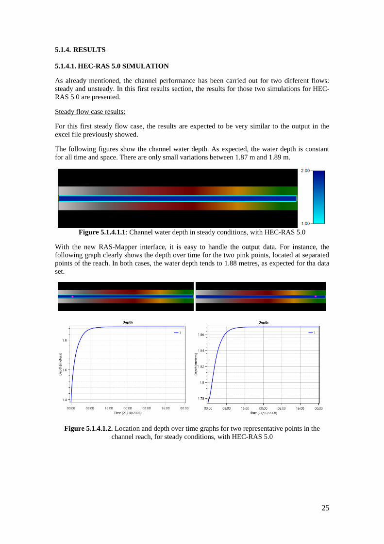
With the new RAS-Mapper interface, it is easy to handle the output data. For instance, the
following graph clearly shows the depth over time for the two pink points, located at separated
points of the reach. In both cases, the water depth tends to 1.88 metres, as expected for tha data
set.
Figure 5.1.4.1.2. Location and depth over time graphs for two representative points in the
channel reach, for steady conditions, with HEC-RAS 5.0

26
As expected in the calculations, the water velocity is very close to 0.43 m/s with only little
variations:
Figure 5.1.4.1.3. Channel water velocity all over the reach for steady conditions,
with HEC-RAS 5.0
The following pink point shows the location for the velocity-time graph. As one can see, the
hyperbolic curve tends to 0.43 m/s, as expected.
Figure 5.1.4.1.4. Location and velocity over time graph for selected point of the ideal channel,
in steady conditions, with HEC-RAS 5.0

27
Unsteady flow case results (flood simulation):
For the purpose of modelling a flood simulation, the channel has been object of the created
hydrological data mentioned in the case description section, which starts in a steady state
(200m3/s) and has a peak discharge of 450m3/s before coming back to the steady state again at
the last part of the time period.
The process of the flow modelled with HEC-RAS 5.0 is the following (units: depth in metres):
20OCT2008 03:00
20OCT2008 10:30
20OCT2008 12:00
20OCT2008 14:00
20OCT2008 17:00
20OCT2008 20:00
20OCT2008 23:00

28
21OCT2008 02:00
21OCT2008 07:00
21OCT2008 12:00
22OCT2008 00:00
Figure 5.1.4.1.5. Flooding flow behaviour series of the ideal channel for the unsteady
hydrological data created, with HEC-RAS 5.0
In sum, the flow starts behaving steadily (20OCT2008 03:00) and then turns unsteady, flooding
the floodplains from the top to the downstream end. After that, the discharge diminishes again
and that’s why the domain starts to dry out (noticeable at the upstream end side in picture
22OCT2008 00:00).
However, a little instability has been noticed. The fact is that two thin longitudinal dry areas,
which were not expected, appear in the slope change between the floodplains and the main
channel when the flow reaches to the downstream region. This is observable in the previous
pictures, from 20OCT2008 23:00 to 22OCT2008 00:00. One can see that those areas are first
short, but start extending until they reach the upstream end.
The cause of this issue could probably be the combination of two facts. First, the water depth at
the flooded areas is really small at the end of the simulation time (less than 10 centimetres),
which can lead to wetting-drying problems, this is, how the program distinguishes whether a
cell is considered wet or not when the water depth value is really small. Second, the area of the
problem is exactly when the channel wall slopes appear. This is obviously an area which is
likely to have instability problems, since its slope is not constant.
The next image shows the area of the problem from a closer point of view.
Figure 5.1.4.1.6. Close view of the area at the downstream end of the reach
at time 21OCT2008 10:45
29
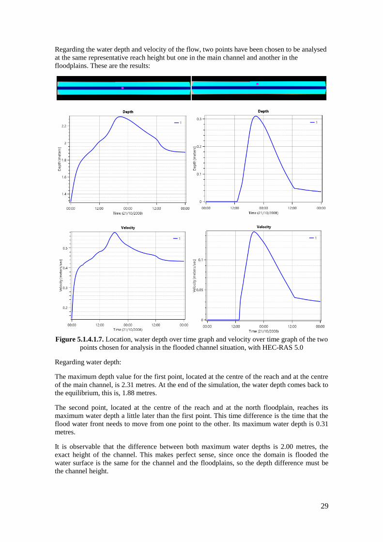
Regarding the water depth and velocity of the flow, two points have been chosen to be analysed
at the same representative reach height but one in the main channel and another in the
floodplains. These are the results:
Figure 5.1.4.1.7. Location, water depth over time graph and velocity over time graph of the two
points chosen for analysis in the flooded channel situation, with HEC-RAS 5.0
Regarding water depth:
The maximum depth value for the first point, located at the centre of the reach and at the centre
of the main channel, is 2.31 metres. At the end of the simulation, the water depth comes back to
the equilibrium, this is, 1.88 metres.
The second point, located at the centre of the reach and at the north floodplain, reaches its
maximum water depth a little later than the first point. This time difference is the time that the
flood water front needs to move from one point to the other. Its maximum water depth is 0.31
metres.
It is observable that the difference between both maximum water depths is 2.00 metres, the
exact height of the channel. This makes perfect sense, since once the domain is flooded the
water surface is the same for the channel and the floodplains, so the depth difference must be
the channel height.

30
Regarding flow velocity:
The first point has its maximum in 0.58m/s while the second has it in 0.15m/s. One also needs
to take into consideration the fact that the water in the channel moves much more longitudinally
than the water in the floodplains, which also moves laterally in order to flood the dry areas. This
is shown in more detail in the Delft3D results.
The magnitude velocity difference between main channel and floodplains can be observed in the
following image. Units in m/s.
Figure 5.1.4.1.8. Water flow velocity difference between the main channel and the two
floodplains in the flooded channel situation (velocity units in m/s), with HEC-RAS 5.0

31
5.1.4.2. DELFT3D SIMULATION
In the present section, the results for steady and unsteady simulations for the ideal channel with
Delft3D are presented.
Steady flow case results:
The steady case results with Delft3D are also notably satisfactory. All the predicted data can be
considered correct.
The following figures show the channel water depth. As expected, the water depth is constant
for all time and space. For this reason only one figure is enough to show the water depth
behaviour in this steady case. On it, one can see the dry floodplains and a water depth of around
1.88 in the main channel.
Figure 5.1.4.2.1. Channel water depth all over the reach in steady conditions, with Delft3D
Or, which is the same, the water level is steady for all simulation times:
Figure 5.1.4.2.2. Channel water level all over the reach in steady conditions, with Delft3D
Velocities are analysed by means of observation points set along the channel reach. In this case,
three observation points are set for results. The exact location of this points is not of relevant
importance in this case since the results need to be steady for all of them.
Figure 5.1.4.2.3. Situation of the three observation points for the steady flow performance in
the channel, with Delft3D

32
The first observation point (44,28) computes a velocity in x-direction (component 1) of 0.42-
0.43 m3/s, while the previous calculations are about 0.43 m3/s. Thus, those calculations can be
considered really accurate.
The second component of the velocity is negligible, as it was assumed in the beginning since
the channel is straight, the flow is steady and the initial transversal velocity input is negligible.
Figure 5.1.4.2.4. Graph showing the two water velocity components over time in the unsteady
channel simulation with Delft3D for point (44,28)
Figure 5.1.4.2.5. Graph showing the magnitude difference between both velocity components
in the unsteady channel simulation with Delft3D for point (44,28)
33
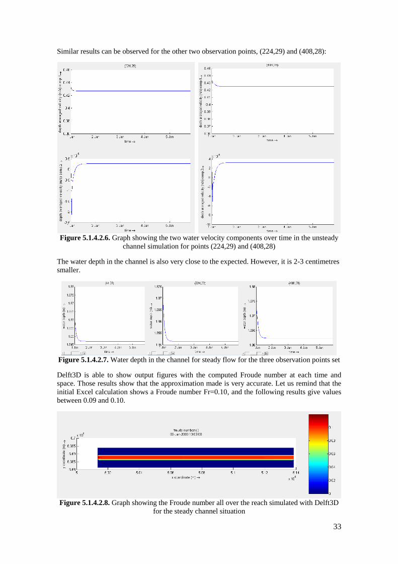
Similar results can be observed for the other two observation points, (224,29) and (408,28):
Figure 5.1.4.2.6. Graph showing the two water velocity components over time in the unsteady
channel simulation for points (224,29) and (408,28)
The water depth in the channel is also very close to the expected. However, it is 2-3 centimetres
smaller.
Figure 5.1.4.2.7. Water depth in the channel for steady flow for the three observation points set
Delft3D is able to show output figures with the computed Froude number at each time and
space. Those results show that the approximation made is very accurate. Let us remind that the
initial Excel calculation shows a Froude number Fr=0.10, and the following results give values
between 0.09 and 0.10.
Figure 5.1.4.2.8. Graph showing the Froude number all over the reach simulated with Delft3D
for the steady channel situation

34
Unsteady flow case results (flood simulation):
The following series of figures represent the water depth on the channel reach. As expected, the
water flows outside the main channel and reaches the floodplains. It is noticeable that the
maximum discharge is released between 16:00h and 18:00h on the 1st of January. It is from that
moment when the floodplains start being seriously flooded.

35
Figure 5.1.4.2.9. Flooding flow behaviour series of the channel for the unsteady hydrological
data created, with Delft3D
One can easily see that the behaviour at the last third of the reach is different. This is
due to the fact that when the water reaches this area, the front wave (maximum
discharge released) is already stabilized, so the water flow that gets there has much less
energy and is not flooding the floodplains so severely. The white area is area which is
never considered wet in the whole process.
This fact can lead to controversy about the reliability of both Delft3D and HEC-RAS
5.0 models, since slight different results appeared. However, this is very likely to be a
mere tolerance issue, this is, one model has different value than the other for
considering a cell to be wet or not. Could be that HEC-RAS 5.0 considers 2mm depth
enough to define that a cell is wet, but Delft3D uses 4mm for that purpose. This leads to
differences in terms of results although the calculations are the same.

36
In order to better analyse the behaviour of the different features of the flow at exact points in the
floodplain, six extra points have been added to the three already used for the previous steady
simulation.
Figure 5.1.4.2.10. Situation of observation points over the channel reach and floodplains for
unsteady results with Delft3D
Regarding water depth results, points (224,43), (224,29) and (224,17) will be analysed. Those
points are especially chosen because they have similar locations to the points in the river reach
analysed for the HEC-RAS 5.0 case.
Water depth results for observation point (224,29) are presented in Figure 5.1.4.2.11.
Figure 5.1.4.2.11. Water depth over time graph of point (224,29) for the flooded channel
situation, with Delft3D
As examples for the floodplains, results on water depth for points (224,43) and (224,12) in the
floodplains are presented below.
One should note that those points are at the same domain height but at opposite floodplains, one
in each side of the main channel. Therefore, symmetric results may be expected for those points
in terms of depth and velocity, taking into account the symmetry of the domain. Regarding to
the depth in particular, the values must be the same at the same time, as follows:
Figure 5.1.4.2.12. Water depth over time graph of points (224,43) and (224,12) for the flooded
channel situation, with Delft3D

37
Regarding the depth averaged velocity results, those can be represented in QUICKPLOT
interface, with arrows that show the magnitude and direction of the water flow.
Figure 5.1.4.2.13. Flow velocity general results for unsteady channel case, with Delft3D
From a closer viewpoint:
Figure 5.1.4.2.14. Close view of flow velocity general results for unsteady channel case, with
Delft3D
Those views, though, are not very clear and are difficult to analyse. In order to properly analyse
the velocity results in the floodplains, one is more interested in analysing the six extra
observation points that have been placed in the area.
As examples, results on velocity for points (224,43) and (224,12) in the floodplains are
presented on the next page. As said, those points are chosen because they have similar locations
as the points in the floodplains analysed for the HEC-RAS 5.0 case. Their graphs show that the
velocity is zero until the floodplain is flooded, as expected. One can also observe that the
transversal velocity component is not negligible as it was happening in the steady flow case,
because in this case the water is flowing laterally too, in order to cover the dry area of the
floodplains.
As expected, due to the symmetry of the domain and the opposite position of the points in the
floodplains, the results show same values for the longitudinal velocity component (component
1) over time and, for the lateral velocity component (component 2), same value magnitudes but
with opposite sign, since the direction of the flow is north for the northern floodplain and south
for the southern floodplain.
The mentioned graph results are shown in the next page.

38
Figure 5.1.4.2.15. Graphs showing the two water velocity components over time and the
relation between them, in the unsteady channel simulation, for point (224,43), with Delft3D
Figure 5.1.4.2.16. Graphs showing the two water velocity components over time and the
relation between them, in the unsteady channel simulation, for point (224,12), with Delft3D
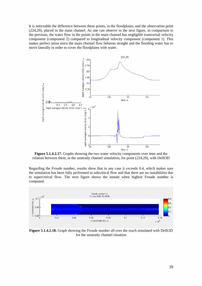
39
It is noticeable the difference between these points, in the floodplains, and the observation point
(224,29), placed in the main channel. As one can observe in the next figure, in comparison to
the previous, the water flow in the points in the main channel has negligible transversal velocity
component (component 2) compared to longitudinal velocity component (component 1). This
makes perfect sense since the main channel flow behaves straight and the flooding water has to
move laterally in order to cover the floodplains with water.
Figure 5.1.4.2.17. Graphs showing the two water velocity components over time and the
relation between them, in the unsteady channel simulation, for point (224,29), with Delft3D
Regarding the Froude number, results show that in any case it exceeds 0.4, which makes sure
the simulation has been fully performed in subcritical flow and that there are no instabilities due
to supercritical flow. The next figure shows the instant when highest Froude number is
computed.
Figure 5.1.4.2.18. Graph showing the Froude number all over the reach simulated with Delft3D
for the unsteady channel situation

40
5.1.5. EXTRA TESTS: M1 AND M2 CURVES
Some more extra tests with HEC-RAS 5.0 have been performed in order to check its
workability when the water surface defines curves M1 and M2 (mild slope curves).
The following figure shows the shape that every type of M curves present:
Figure 5.1.5.1. M-type curves (Gutiérrez, 2014)
where y0 is the normal water depth and yc is the critical water depth
For this purpose, the same previous steady case data has been applied, with the only difference
of varying the downstream boundary condition. Since the critical depth has been proved to be
1.88 metres, one would need a higher value in order to get an M1 curve and a smaller value for
an M2 curve. Those values have been set as 2 m and 1 m respectively.
Table 5.1.5.1. Boundary conditions set for the M1 and M2 curves in the channel, with HEC-
RAS 5.0
M1 CURVE M2 CURVE
Upstream
BC
Steady discharge: 200 m3/s Steady discharge: 200 m3/s
Downstream
BC
Water depth 2 m Water depth 1 m
Curve searched

41
M1 curve results
The results show the expected gradient of water depths, starting from around 1.89 - 1.88 metres
(very close to the normal depth for the discharge applied and critical depth at the same time) at
the upstream end and growing up the level until 2 metres water depth at the downstream end.
Figure 5.1.5.2.Water depth in the case of M1 curve in the channel. Units in metres.
Therefore, if depth increases in downstream direction, flow velocity must decrease in the same
direction, according to the equation 𝑢 =𝑞
𝑑, where u is the flow velocity, q is the discharge over
width and d is the water depth. The following figure with the flow velocity results are showing
exactly this phenomena:
Figure 5.1.5.3. Flow velocity in the case of M2 curve in the channel. Units in metres.
M2 curve results
The results show the expected gradient of water depths, starting from 1.88 metres (normal depth
for the discharge applied and critical depth at the same time) at the upstream end and lowering
the level until 1 metre water depth at the downstream end.
Figure 5.1.5.4. Water depth in the case of M2 curve in the channel. Units in metres.
Therefore, if depth decreases in downstream direction, flow velocity must increase in the same
direction. Again, the following figure with the flow velocity results are showing exactly this
phenomena:
Figure 5.1.5.5. Flow velocity in the case of M2 curve in the channel. Units in metres.
In sum, these extra tests regarding M-type curves have led to the expected results.
After this series of simulations, it is concluded that the workability basics with HEC-RAS 5.0
have been learnt and that the next sections can already handle more complex simulation
scenarios.
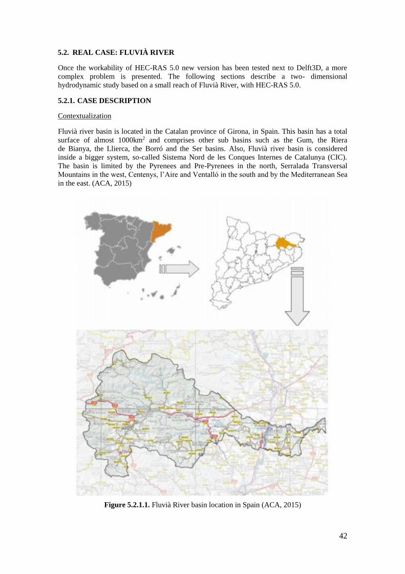
42
5.2. REAL CASE: FLUVIÀ RIVER
Once the workability of HEC-RAS 5.0 new version has been tested next to Delft3D, a more
complex problem is presented. The following sections describe a two- dimensional
hydrodynamic study based on a small reach of Fluvià River, with HEC-RAS 5.0.
5.2.1. CASE DESCRIPTION
Contextualization
Fluvià river basin is located in the Catalan province of Girona, in Spain. This basin has a total
surface of almost 1000km2 and comprises other sub basins such as the Gum, the Riera
de Bianya, the Llierca, the Borró and the Ser basins. Also, Fluvià river basin is considered
inside a bigger system, so-called Sistema Nord de les Conques Internes de Catalunya (CIC).
The basin is limited by the Pyrenees and Pre-Pyrenees in the north, Serralada Transversal
Mountains in the west, Centenys, l’Aire and Ventalló in the south and by the Mediterranean Sea
in the east. (ACA, 2015)
Figure 5.2.1.1. Fluvià River basin location in Spain (ACA, 2015)

43
Fluvià River longitude is 100km, originating in La plana d’en Bas, at 920m altitude, and
ending up at the sea, in Gulf of Roses, close to the small village of Sant Pere Pescador. Its
trajectory passes by close to Olot, Sant Joan de les Fonts, Castellfollit de Roca, Besalú,
Esponellà and Torroella de Fluvià, this is, mainly Garrotxa, Pla de l’Estany and Alt Empordà
regions. (ACA, 2015)
Figure 5.2.1.2. Fluvià River reaches and sub basins (ACA, 2015)
Nevertheless, the area of study is only a little reach of Fluvià River, located next to Torroella de
Fluvià. The following image shows in more detail the investigation site.
Figure 5.2.1.3. Domain studied, top view satellite image (Google Maps, 2015)
44
Initial data
The initial data for the Fluvià river reach simulation consists in:
- The topography of the domain (see picture in the previous page), which consists in a text
file (.txt) with data of 5x5m2 cell size that covers the full domain (546 columns and 249
rows). Thus, the domain measures are 2730x1245m2.
- Hydrological data, based on the total discharge data at the upstream end, given by Agència
Catalana de l’Aigua (ACA, Catalan Water Agency) in July 2009.
Some problems appeared due to the upstream end hydrological data. At first, this data was
given for a return period of 500 years (peak total discharge of 3400m3/s). However, when
running the program, an error appeared, saying that the water level was rising to more than 25
meters in a very short period of time, which is not possible in a realistic performance. The
problem was that this discharge was definitely too severe for the small domain and the
consequence was that, when the flood reached the domain limits, those limits behaved like walls
and the full domain was filled with water, like a swimming pool.
Once the problem was noticed, the hydrological data was changed from 500 to 10 years of
return period (with a peak discharge of 400m3/s). This new discharge first resulted in a proper
flooding simulation with a time step of 1 minute, which let us think the simulation would be
definitive. However, after contrasting HEC-RAS 5.0 and an IBER simulation performed by the
director of this project, Martí Sánchez-Juny, it was noticed that the time step was too high and
that the result was not realistic, since the mentioned discharge would not be enough to flood the
area. The time step value was then set to 0.25 minutes (15 seconds) and, as expected, a non-
flooded situation was the result. Those “erroneous” simulations are also present in the results
section for a better understanding of the reader about the process.
Finally, the discharge data was changed again in order to flood the area. This time, the return
period chosen was of 50 years, relative to a maximum total water discharge of around 1200m3/s.
This discharge magnitude was definitely more appropriate for the case, since no conceptual
errors appeared and the domain was flooded as expected. The results were successfully checked
again with IBER.
In the results sections, not only the definitive simulation (T=50 years) but also the non-flooded
ones (T=10 years) are analysed. Thus, in the end, three simulations are presented:
- Simulation 1: T=10 years, Δt=1 minute. “Erroneous” simulation.
- Simulation 2: T=10 years, Δt=0.25 minute. “Non-flooded” simulation.
- Simulation 3: T=50 years, Δt=0.25 minute. “Flooded” simulation.
The hydrological data obtained for the performance of the mentioned simulations follows in the
next page.

45
Figure 5.2.1.4. Fluvià hydrograph for T=10 years Figure 5.2.1.5. Fluvià hydrograph for T=50 years
Table 5.2.1.1. Hydrograph data for T=10 years Table 5.2.1.2. Hydrograph data for T=50 years
(ACA, 2009) (ACA, 2009)
Date Time Discharge (m3/s) Date Time Discharge (m3/s)
20-oct-08 0:00 0 20-oct-08 0:00 0
20-oct-08 7:00 8.3 20-oct-08 7:00 38.6
20-oct-08 8:00 21.8 20-oct-08 8:00 84.9
20-oct-08 9:00 30.2 20-oct-08 9:00 126
20-oct-08 10:00 39.1 20-oct-08 10:00 147.7
20-oct-08 11:00 41.9 20-oct-08 11:00 136.2
20-oct-08 12:00 41.6 20-oct-08 12:00 115.2
20-oct-08 13:00 38.9 20-oct-08 13:00 404.4
20-oct-08 14:00 43.9 20-oct-08 14:00 612.8
20-oct-08 15:00 129.3 20-oct-08 15:00 789.5
20-oct-08 16:00 397.2 20-oct-08 16:00 1123.6
20-oct-08 17:00 386.4 20-oct-08 17:00 1197
20-oct-08 18:00 332.5 20-oct-08 18:00 1075.4
20-oct-08 19:00 279.7 20-oct-08 19:00 900.6
20-oct-08 20:00 234.1 20-oct-08 20:00 489.4
20-oct-08 21:00 195 20-oct-08 21:00 299.7
20-oct-08 22:00 161.2 20-oct-08 22:00 221.5
20-oct-08 23:00 131.8 20-oct-08 23:00 168.5
21-oct-08 0:00 106.9 21-oct-08 0:00 123.8
21-oct-08 1:00 86.2 21-oct-08 1:00 88.5
21-oct-08 2:00 68.5 21-oct-08 2:00 60
21-oct-08 3:00 52.4 21-oct-08 3:00 39.6
21-oct-08 4:00 36.1 21-oct-08 4:00 26.8
21-oct-08 5:00 19.7 21-oct-08 5:00 18.6
21-oct-08 6:00 10.3 21-oct-08 6:00 12.3
21-oct-08 7:00 5.8 21-oct-08 7:00 7.1
21-oct-08 8:00 3.5 21-oct-08 8:00 3.8
21-oct-08 9:00 2.1 21-oct-08 9:00 2
22-oct-08 0:00 0 21-oct-08 0:00 0

46
5.2.2. CONSIDERATIONS
The case study site has some characteristics and considerations that must be understood before
reading the results of the simulation performance.
Roughness coefficient
Manning’s coefficient of roughness has been considered n=0.035. This value has been extracted
from a morphodynamic study of “Planificació de l’espai fluvial de la conca del Fluvià”, by
ACA. The same value is applied to both the river bed and floodplains, for simplification issues.
Downstream boundary condition
With HEC-RAS 5.0, the user can set a “Normal depth” in the downstream boundary condition.
This feature works by means of a “warming up time”, formally called initial conditions time, in
which the model “warms up” for some time in the beginning of the simulation in order to set a
normal depth at the downstream end. This methodology has been applied in this case, with an
initial conditions time of one hour.
Thin dam
The reach of study contains a thin dam, located in the centre of the domain. Some
hydrodynamic models include the option to add thin dams to the simulation reach. This is
possible, for instance, in models like Delft3D. However, not only this feature has not been
applied in the case simulation, but also it would have been wrong to apply it, since the
topography data is already considering the terrain elevation at the dam points, so the program
already takes that into account.
Bridge
There is a road bridge that crosses the reach of study. Sometimes, for very precise simulations,
one can consider the influence of the bridge piles in the water flow. This can be applied in
models like Delft3D using the option Dry points, for instance. However, for simplification, this
effect has been considered negligible in the simulations of this document.
a b
Figure 5.2.2.1. a) Thin dam top view (Google Maps, 2015)
b) Bridge top view (Google Maps, 2015)
Latitude for Coriolis
In order to take into account the Coriolis forces, the real value for the latitude of the real case
study is set, this is, 42.17 degrees.

47
5.2.3. PERFORMANCE
HEC-RAS 5.0 simulation functionality
In brief summary, the steps applied for HEC-RAS 5.0 simulation are the following:
- Input topography from text file with RAS Mapper
- Grid creation with Geometry data window
o Define area
o Define cell size: 5x5m2
o Define Boundary condition lines
- Flow definition in Unsteady flow data edition
o Flow hydrograph at upstream boundary condition
o Normal depth at downstream boundary condition
- Run simulation
- Analyse results
Calculation grid
The calculation grid of study is a rectangular grid with by 5x5m2 squared cells. In this case, the
mesh has been created with 82328 cells. This is a notably detailed mesh taking into account the
small domain and the apparent simplicity of the problem.
Figure 5.2.3.1. Terrain with the mesh and boundaries applied, with HEC-RAS 5.0
Figure 5.2.3.2. Mesh and boundaries used for Fluvià River reach, with HEC-RAS 5.0

48
Figure 5.2.3.3. Detailed view for mesh with squared cells used
5.2.3.1. PROBLEMS FOUND
During the performance of the real case simulation, some obstacles that led to an increase of the
expected work time were found.
Regarding data input:
- The data initially received consisted of the topography of the area and the hydrograph for
a return period of 500 years. As previously explained, since the total discharge for 500
years of return period is huge, the water was reaching the limits of the (small) domain.
This would not be a problem if it was not because the program considers the limits as
vertical walls by defect, so the resulting simulation was a “full swimming pool”, with no
technical or hydrodynamic interest for us. Since it was difficult to notice what was
happening, why did it show an error, this obstacle led to a big loss of time. The solution
was to change the hydrological data from 500 to 10 years of return period, so that the
domain was not completely filled with water. This data was finally changed again to a
return period of 50 years.
Regarding simulation performance:
- The initial time step set was 1 minute. This led to a too high Courant number (CFL),
situation in which lots of numerical instabilities arise. In consequence, Simulation 1
modelled a flooding scenario when there was actually no flood for the hydrological
data introduced. As explained, the next simulation was performed with a time step of
15 seconds, which solved this instability problems.

49
5.2.4. RESULTS
Simulation 1: T=10 years, Δt=1 minute. “Erroneous” simulation.
As mentioned in section 3.2.2.1, at first, the flooded situation simulation was thought to be
correct with hydrological data of a return period of 10 years. However, it was not, since the time
step applied was 1 minute and had to be lowered until 0.25 minutes, this is, 15 seconds, which
led to different results, showing flooding where, in reality, there was not. Although this can be
considered a mistaken simulation, the results are shown for a better understanding about what
happened.
The following series of images show the water depth behaviour for this simulation over time.
One can easily distinguish a flooding behaviour of the flow.

50
Figure 5.2.4.1. Flooding flow behaviour series of Fluvià River simulation 1 with HEC-RAS 5.0
According to IBER simulation checks, this observable flooding situation was not realistic, since
the hydrological data applied, with a peak discharge of around 400m3/s was not supposed to
results in such a severe flood in the area.
It was then concluded that there were instabilities due to a too high Courant number (CFL).
Thus, the time step was reduced for the next performances.

51
Simulation 2: T=10 years, Δt=0.25 minute. “Non-flooded” simulation.
After realising the previous simulation was erroneous, the time step was switched from
Δt=1min to Δt=0.25min. This change let us notice that the flow scenario for a hydrological data
of a return period f 10 years was not at all a flood.
The following series of images show the water depth behaviour for this simulation over time.
One can easily distinguish a non-flooding behaviour of the flow.
Figure 5.2.4.2. Non-flooding flow behaviour series of Fluvià River simulation 2,
with HEC-RAS 5.0
The four firsts pictures show how the Fluvià River gets full of water in its main river channel. In
the fifth, the peak water discharge fill it completely but, contrary to first expectations, cannot
reach the floodplains. Finally, the last picture shows how the river dries out.

52
Simulation 3: T=50 years, Δt=0.25 minute. “Flooded” simulation.
After realising the previous simulation describes a non-flooding situation, the hydrological data
has been changed in order to simulate a flood in the channel floodplains. The new hydrological
data corresponds to a return period of 50 years, obtained by Agència Catalana de l’Aigua
(ACA) in 2009. This is the definitive and previously wanted simulation: a realistic simulation of
a flood situation in Fluvià River and the sorrounding area.
Three main stages can be distinguished in the flow progress of Simulation 3.
One first stage in which the water appears from the upstream end and fills the river main
channel. This stage comprises the times from the simulation start time, 20OCT2008 00:00, to
20OCT2008 12:30, when the water flow starts flooding the floodplains.
The second stage is the flooding of the floodplains itself, the main objective of this simulation.
The flooding stage develops from 20OCT2008 12:30 to 20OCT2008 19:00. This period of time
is exactly when the most part of the total discharge is released. Thus, it makes perfect sense that
the flood occurs by then. Also, it is noticeable that the northern floodplain is fully inundated but
not the southern one. This may be because of topography issues, this is, the ground level in the
northern side is slightly lower than in the south side, and also because of the river bend, that
makes the water reach the northern floodplain more easily due to forces of inertia.
Since 20OCT2008 19:00 until the end of the simlation, the floodplain surfaces start drying out
until most of the wet parts end up being dried, also in the main channel area. This drying out
step is the third relevant stage of the simulation.
The following two pages show Figure 5.2.4.3, series of images where the water depth behaviour
for this simulation over time can be observed. One can easily distinguish the flooding behaviour
of the flow.
Furthermore, other aspects of the simulation results are explained in detail.

53

54
Figure 5.2.4.3. Flooding flow behaviour series of Fluvià River simulation 3 with HEC-RAS 5.0

55
Regarding the maximum depth, the floodplains are flooded until a depth of around 0.40 to 0.60
metres, which can be considered as a notable flood situation.
Figure 5.2.4.4. Maximum water depths at Fluvià River reach in Simulation 3, with RAS
Mapper interface. Units in metres.
Regarding flow velocity, one can tell there have been some instability errors if one checks the
maximum flow velocities with RAS Mapper interface. The results show, in some points, very
high velocities, which are impossible in a real situation. Those errors arise when we found very
small water depths, since the velocity calculation is 𝑢 =𝑞
𝑑, where u is the flow velocity, q is the
discharge over width and d is the water depth. Thus, for very small values of the water depth,
the flow velocity becomes really high. Besides that, the velocity values along the reach are, in
general, realistic.
Observation: note that this high unrealistic values of the velocity are shown, for instance, on top
of the thin dam, which makes perfect sense since the water depth at those points is really low.
Figure 5.2.4.5. Maximum flow velocities at Fluvià River reach in Simulation 3 with RAS
Mapper interface. Units in m/s.
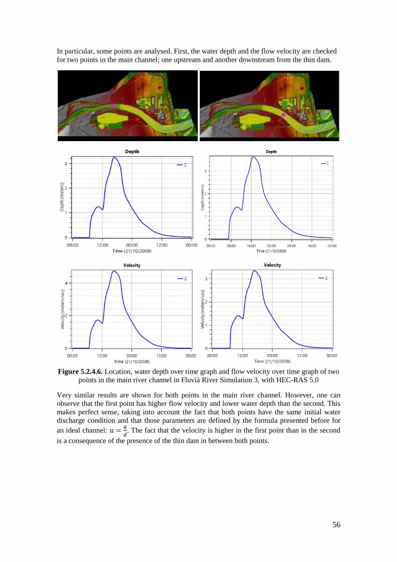
56
In particular, some points are analysed. First, the water depth and the flow velocity are checked
for two points in the main channel; one upstream and another downstream from the thin dam.
Figure 5.2.4.6. Location, water depth over time graph and flow velocity over time graph of two
points in the main river channel in Fluvià River Simulation 3, with HEC-RAS 5.0
Very similar results are shown for both points in the main river channel. However, one can
observe that the first point has higher flow velocity and lower water depth than the second. This
makes perfect sense, taking into account the fact that both points have the same initial water
discharge condition and that those parameters are defined by the formula presented before for
an ideal channel: 𝑢 =𝑞
𝑑. The fact that the velocity is higher in the first point than in the second
is a consequence of the presence of the thin dam in between both points.

57
Also, two information points have been set in the floodplains in order to get some
output about the flooding behaviour of this simulation. Both points are located at the
northern floodplain since the opposite floodplain has not been fully flooded.
Figure 5.2.4.7. Location, water depth over time graph and flow velocity over time graph of two
points in the northern floodplain in Fluvià River Simulation 3, with HEC-RAS 5.0
The results show negligible values until the water discharge reaches the area, which is a little
after than in the main channel case, for obvious reasons. One can observe much smaller
velocities and depths, which is characteristic in the floodplain regions. However, the depth is
considerable during the flooding period, reaching until more than 0.5 metres in a considerable
floodplain area.
Therefore, the studied reach can be considered as an easy-floodable area for hydrological data
related to a return period of 50 years.

58
5.2.5. CONTRAST WITH IBER
All the previous simulation results for Fluvià River reach have been contrasted with simulation
results made with IBER, obtained from the director of this project, Prof. Martí Sánchez-Juny.
This IBER simulation has been performed with the only purpose of contrasting the results of
this paper.
Of course, the boundary conditions applied are the same as in the HEC-RAS 5.0 simulation
performed before, in order to obtain comparable results. A discharge related to the data obtained
from ACA, regarding a return period of 50 years, has been applied at the upstream end
condition, while the critical depth has been set as a downstream boundary condition.
One can compare this results to the HEC-RAS 5.0 simulation results and observe clear
similarities. Again, the major part of the flooded area comprises the northern floodplain. Flow
velocities are higher right before the thin dam, just as it was happening in the HEC-RAS 5.0
performance.
One can state that the last simulation results of this document have been successfully contrasted
with another simulation of the same situation, performed by experts, with a comparable
program, IBER. Therefore, the two-dimensional river flood simulation performed with HEC-
RAS 5.0 in the Fluvià River reach for the obtained hydrological data related to a return period
of 50 years is considered successful.
Figures with the results of maximum depths, maximum water levels and maximum velocities
obtained with IBER are presented.
Figure 5.2.5.1. Maximum depths in Fluvià River simulation obtained with IBER
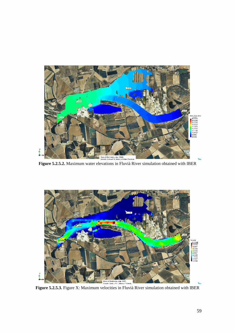
59
Figure 5.2.5.2. Maximum water elevations in Fluvià River simulation obtained with IBER
Figure 5.2.5.3. Figure X: Maximum velocities in Fluvià River simulation obtained with IBER

60
5.3. OVERVIEW OF THE SIMULATIONS PERFORMED
Once all the simulations have been successfully performed, a table of analysis has been
considered useful in order to have an objective overview of the work.
Table 5.3.1. Overview table of the simulations performed
Case Ideal case: Prismatic channel Real case: Fluvià River
Model HEC-RAS 5.0 Delft3D HEC-RAS 5.0
Simulation - - - - Simulation 1 Simulation 2 Simulation 3
Flow Steady Unsteady Steady Unsteady Unsteady Unsteady Unsteady
Grid Rectangular Rectangular Rectangular Rectangular Shaped Shaped Shaped
Cells Squared
25x25m2
Squared
25x25m2
Squared
25x25m2
Squared
25x25m2
Squared
5x5m2
Squared
5x5m2
Squared
5x5m2
Time step used 6s 6s 6s 6s 1min 15s 15s
Initial
situation
Use of
warming
time
Use of
warming
time
Initial
conditions
file
Initial
conditions
file
Use of
warming
time
Use of
warming
time
Use of
warming
time
Upstream BC Created
constant
discharge
200m3/s
Created
unsteady
discharge
(peak
450m3/s)
Created
constant
discharge
200m3/s
Created
unsteady
discharge
(peak
450m3/s)
Hydrological
data by APA
T=10 years
Hydrological
data by APA
T=10 years
Hydrological
data by APA
T=50 years
Downstream
BC
Water level
1.87 m
Water level
1.87 m
Water level
1.87 m
Water level
1.87 m
Normal
depth
Normal
depth
Normal
depth
Roughness
coefficient
Manning
n=0.035
Manning
n=0.035
Manning
n=0.035
Manning
n=0.035
Manning
n=0.035
Manning
n=0.035
Manning
n=0.035
Equations Full
momentum
Full
momentum
Full
momentum
Full
momentum
Diffusive
wave
Full
momentum
Full
momentum
Latitude for
Coriolis
0 deg 0 deg 0 deg 0 deg 42.17 deg 42.17 deg 42.17 deg
Flooding
behaviour
No Yes No Yes Yes
(erroneous)
No Yes
Computational
time
1h16min 1h17min 29min 14min 45min 4h05min 4h17min
Fr<1 Yes Yes Yes Yes Yes Yes Yes

61
6. CONCLUSIONS
Conclusions regarding the initial purposes and research questions can be extracted from the
different parts of this paper.
From the intercomparison between the main hydrodynamic numerical models, this is, between
HEC-RAS 5.0, Delft3D, IBER, SOBEK and 3Di, the following conclusions can be extracted:
- The most important features to consider when comparing hydrodynamic models are:
dimensions, hydrodynamic equations, numerical equations resolution method, hydraulic
roughness, turbulence submodels, suitability for supercritical flow, structures,
combination with transport of substances and water quality, combination with sediment
transport and morphological evolution, local running availability and open source
availability.
- The most important features to consider when comparing hydrodynamic models regarding
river flood modelling are: dimensions, hydrodynamic equations, numerical equations
resolution method, hydraulic roughness, turbulence submodels, suitability for supercritical
flow, structures and local running availability.
- HEC-RAS 5.0 is definitely comparable to the main hydrodynamic models in use.
- Delft3D and SOBEK were appropriate models to compare to HEC-RAS 5.0 from a
practical approach in this paper.
- Although all the models studied are able to perform realistic river flood simulations, they
all have different features and work differently.
From the study comparison in two-dimensional numerical modelling of the hydrodynamic
behaviour of an ideal prismatic channel reach between HEC-RAS 5.0 and Delft3D, created for
the only purpose of this document in an imaginary environment, with created hydrological data,
the following conclusions can be extracted:
- HEC-RAS 5.0 presented a little instability in the unsteady flooding case, resulting in two
thin longitudinal dry areas at the slope change between the floodplains and the levees.
This is not considered a major error but it is of interest to report.
- Delft3D presented a notable dry area at the last third of the reach, in the floodplains,
where there was supposed to be water with very small depth values. This can be due to
tolerance issues with not further importance, as explained in the simulation results section.
- HEC-RAS 5.0 computational time is in general higher than for Delft3D for same exact
situations.
- Both models performed realistic simulations of the two situations proposed, this is, for
steady non-flooding and unsteady flooding cases for the same prismatic channel, although
they have different workability and presented slightly different results.
From the study in two-dimensional numerical modelling of the hydrodynamic behaviour of
Fluvià River reach in the environment of Torroella de Fluvià, for hydrological data concerning a
period of return of 50 years, using HEC-RAS 5.0, the following conclusions can be extracted:
- The studied area is an easily-floodable terrain for 50 years of return period data.
- The maximum water depth range found in the floodplains is between 0.5 and 0.7 m, which
is considerable taking into account the small magnitude of Fluvià River annual discharge
and that the data is related to a return period of only 50 years.
- The maximum water velocity range found in the floodplains is between 0.7 and 1.3 m/s.
- The maximum water velocity range found in the river is between 4.5 and 5.5 m/s at the
area before the thin dam. Downstream from the thin dam and in consequence of it,
velocities decrease notably. Note: the error explained in the next point is not considered
for these velocity results data.
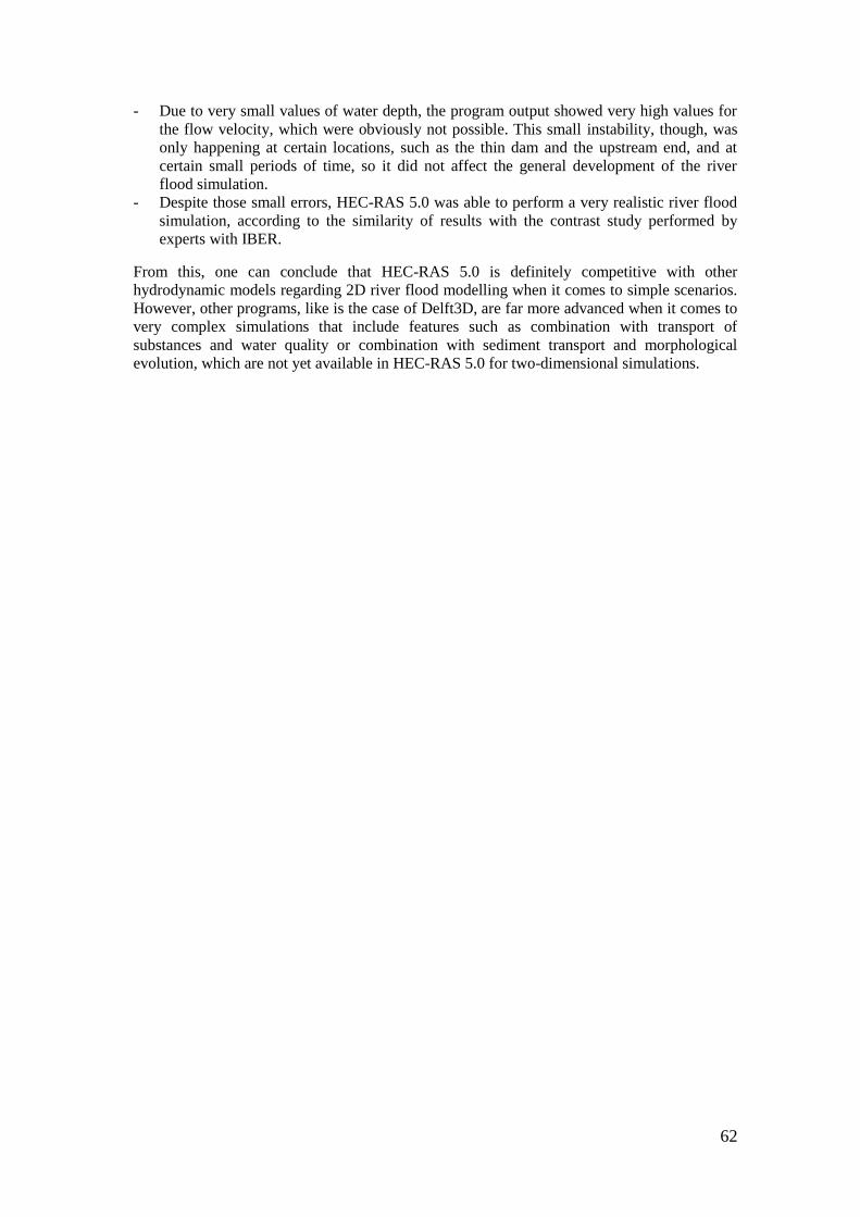
62
- Due to very small values of water depth, the program output showed very high values for
the flow velocity, which were obviously not possible. This small instability, though, was
only happening at certain locations, such as the thin dam and the upstream end, and at
certain small periods of time, so it did not affect the general development of the river
flood simulation.
- Despite those small errors, HEC-RAS 5.0 was able to perform a very realistic river flood
simulation, according to the similarity of results with the contrast study performed by
experts with IBER.
From this, one can conclude that HEC-RAS 5.0 is definitely competitive with other
hydrodynamic models regarding 2D river flood modelling when it comes to simple scenarios.
However, other programs, like is the case of Delft3D, are far more advanced when it comes to
very complex simulations that include features such as combination with transport of
substances and water quality or combination with sediment transport and morphological
evolution, which are not yet available in HEC-RAS 5.0 for two-dimensional simulations.

63

64
7. REFERENCES
ACA: Agència Catalana de l'Aigua. (2015). Sitio web: http://aca-
web.gencat.cat/aca/documents/ca/publicacions/espais_fluvials/publicacions/estudis_pef/c_fluvia
/pef_fluvia.htm#fragment-01
Bladé, E., Cea, L., Corestein, G., Escolano, E., Puertas, J., Vázquez‐Cendón, M.E., Dolz, J., Coll, A.
(2014). Iber: herramienta de simulación numérica del flujo en ríos. Revista Internacional de
Métodos Numéricos para Cálculo y Diseño en Ingeniería, Vol.30(1) pp.1‐10
Bladé, E., Corestein, G., Cea, L., Lara, A., Escolano, E., Coll, A. (2014). Iber, a river dynamics simulation tool. Barcelona, Spain: UPC.
Bladé, E., Lluén, W. E. (2015). Aplicación de la nueva herramienta HEC-RAS 5.0 para cálculos
bidimensionales del flujo de agua en ríos. Barcelona, Spain: UPC.
Bladé, E., Sánchez-Juny, M. (2010). Estudi en model numèric bidimensional del funcionament
hidràulic del riu Fluvià a l'entorn de Torroella de Fluvià considerant el condicionament de la carretera C-31. Barcelona, Spain: FLUMEN, E.T.S. d'Enginyers de Camins, Canals i Ports, UPC.
Bladé, E., Sánchez-Juny, M., Sánchez, H.P., Gómez, M. (2009). Modelación numérica en ríos en
régimen permanente y variable. Una visión a partir del modelo HEC-RAS. Barcelona, Spain:
Edicions UPC.
Blom, A. (2015). River Engineering Lecture Notes. Delft, The Netherlands: Faculty of Civil
Engineering and Geosciences, Technical University of Delft.
Brunner, G. W. (2014). Combined 1D and 2D Modeling with HEC-RAS.
Cáceres, E.D. (2006). Modelación numérica del Río Huancabamba en la zona del Embalse Limón.
Piura, Perú: Universidad de Piura, UDEP.
Deltares. (2014). Delft3D-FLOW User Manual. Delft, The Netherlands: Deltares.
Deltares. (2016). SOBEK, Hydrodynamic, Rainfall Runoff and Real Time Control User Manual.
Delft, The Netherlands: Deltares.
European Comission.(2015). EU Floods Directive. Website: ec.europa.eu/environment/water/flood_risk
Flumen, Grupo de Ingeniería del Agua y del Medio Ambiente. (2014). Modelización bidimensional del flujo en lámina libre en aguas poco profundas. Barcelona, Spain.
Gilles, D., Moore, M. (2010). Review of Hydraulic Flood Modeling Software used in Belgium, The
Netherlands and the United Kingdom. Iowa, USA: University of Iowa, College of Engineering.
Google Maps. (2015) [Map of Torroella de Fluvià and surroundings, Catalonia, Spain]. Website:
https://www.google.es/maps
Gutiérrez, C. (2014). Apuntes de Hidráulica. Barcelona, Spain: E.T.S. d'Enginyers de Camins,
Canals i Ports, UPC.
Johansson, M. (2012). Evaluation of RANS turbulence models for the hydrodynamic analysis of an
axisymmetric streamlined body with special consideration of the velocity distribution in the stern region. Stockholm, Sweden: KTH Royal Institute of Technology.
Moffatt and Nichol (2005). Hydrodynamic modeling tools and techniques. South Bay Salt Pont
Restoration Project. California, USA: Coastal Conservancy.
NOAA Office of Coast Survey (2015). How Hydrodynamic Models Are Used. Website:
http://www.nauticalcharts.noaa.gov/csdl/learn_models.html

65
O’Connor, J.E., Costa, J.E. (2004). The World’s Largest Floods, Past and Present: Their Causes
and Magnitudes. Denver, USA: U.S. Geological Survey.
Pedrozo-Acuña, A., Torres-Freyermuth, A. (2011). Sobre el uso de las ecuaciones de Navier-Stokes
con el promedio de Reynolds en el campo de la ingeniería de costas. Yucatán, México: Instituto de
Ingeniería, Universidad Multidisciplinaria de Docencia e Investigación.
The Ras Solution, The place for HEC-RAS members. (2016). Website:
http://hecrasmodel.blogspot.nl/
UPC, Departament d'Enginnyeria Hidràulica, M. i A. (2010). Estudi morfodinàmic del riu
Fluvià. Agència Catalana de l'Aigua. Website: http://aca-
web.gencat.cat/aca/documents/ca/publicacions/espais_fluvials/publicacions/altres_estudis/040P
0001/aca_pef2015c_02B02_estudi_morfodinamic_v1.pdf
US Army Corps of Engineers. (2016). HEC-RAS River Analysis System User's Manual, version 5.0.
California, USA.
US Army Corps of Engineers. (2016). HEC-RAS River Analysis System Hydraulic Reference Manual, version 5.0. California, USA.
US Army Corps of Engineers. (2016). HEC-RAS River Analysis System 2D Modeling User’s
Manual, version 5.0. California, USA.
US Army Corps of Engineers. (2016). HEC-RAS 5.0.1 River Analysis System Release Notes.
California, USA.
US Army Corps of Engineers. (2016). HEC-RAS River Analysis System Applications Guide, version 5.0. California, USA.
3Di Waterbeheer consortium. (2014). 3Di explained. Delft, The Netherlands
3Di Waterbeheer consortium (2015). Website: http://www.3di.nu/en/product-information-2/

66