skjalg erdal 1 dept. of chemistry, centre for materials science and nanotechnology,

Skjalg Erdal1

Dept. of Chemistry, Centre for Materials Science and Nanotechnology, University of Oslo,

FERMIO, Gaustadalleen 21, NO-0349 Oslo, [email protected]

Mixed conduction

Outline• Defects• Derivation of flux equations• Flux of a particular species• Fluxes in a mixed proton, oxygen ion, electron conductor• Fluxes in a mixed proton, electron conductor

– Various defect situations• Fluxes in a mixed proton, oxygen ion conductor• Some materials of interest• Potential issues

Defects

Defects are crucial to the functional properties of materials

Provide paths for transport

Provide traps for other species

Alters the solubility of alien species

Act as donors/acceptors

Become dominating migrating species themselves

Defects

Defects typically dealt with:

Oxygen vacancies: Vo¨

Oxygen interstitials: Oi´´

Hydroxide ion on oxygen site: OHo˙

Metal vacancies: VM´´

Metal interstitials: Mi¨

Addition of aliovalent element to structure: CaLa´

Electronic defects: e´ and h˙

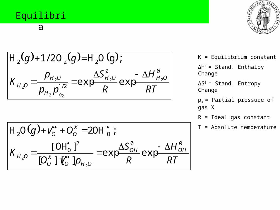
Equilibria

K = Equilibrium constant

ΔH0 = Stand. Enthalpy Change

ΔS0 = Stand. Entropy Change

pX = Partial pressure of gas X

R = Ideal gas constant

T = Absolute temperature

RT

H

R

S

pp

pK

gg

OHOH

H

OHOH

O

00

2/1

222

22

22

2

2expexp

;gOHO2/1H

RT

H

R

S

pvOK

Ovg

OHOH

OHOXO

OH

XOO

002O

O2

expexp]][[

][OH

;OH2OH

2

2

Transport of charged species

xFz

xcB

xcB

x

PcBj i

iii

iii

iiii d

d

d

d

d

d

d

d

Nernst-Einstein:

RT

DcFzBcFzFcz iiiiiiiiii

22

xFz

xFzj i

i

i

ii d

d

d

d2

xFz

xFzFjzi i

i

i

iiii d

d

d

d

ji = flux density

Bi = mech. mobility

ci = concentration

zi = elem. charge

F = Faradays const.

μi = chem. potential

φ = el. potential

σi = conductivity

Di = diff. coefficient

ii = current density


),0(d

d

d

dcircuitopenat

xFz

xFzFjzi

kk

k

k

k

kkktot

Then, use the definition of total conductivity and transport number to find an expression for the electrical potential gradient in terms of transport numbers and chemical potential gradient of all charge carriers:

k

ktot

kk

k

tot

kkt

k

k

k

k

dx

d

Fz

t

dx

d

and


We now need to represent the chemical potential of charged species as the chemical potential of their neutral counterparts.

Assume chemical equilibrium between neutral and charged species and electrons, the electrochemical red-ox reaction:

zeEE z E ~ neutral chemical entity, z ~ + or -

Equilibrium expression is in terms of products and reactants:

eEE

zddd Z Substitute into expression for dx

d

The chemical potential for the neutral species can be expressed via activities, or partial pressures.

dx

d

Fdx

d

Fz

t

dx

d e

n

n

n

n

1 1k

kt,

Voltage over the sample: assume no gradient in electron chemical potential last term becomes zero.


xFz

xFzj i

i

i

ii d

d

d

d2

k

k

k

k

dx

d

Fz

t

dx

d

k

k

k

ki

i

i

ii xz

tz

xFzj

d

d

d

d2

Calculate flux density of species i, in the company of other species

Represents the flux at a particular point in the membrane.

II

I2

II

I

ddk

kk

kii

i

iii z

tz

FzLjdxj

We need the steady state condition constant flux everywhere in membrane

II

I2 dd

1

kk

k

kiii

i

i z

tz

FzLj


II

I2 dd

1

kk

k

kiii

i

i z

tz

FzLj

Expression for SS flux.

Still with chemical potentials of charged species substitute in expressions for neutrals

nd Corresponding neutral species

II

I2 dd

1

nn

n

niini

i

i z

tz

FzLj

kd All charged species

II

I2 dd

1

nn

n

niini

i

i z

tz

FzLj

Fluxes in mixed H+, O2-, el-conductors

Possible contributions to proton transport:

Hnd eHt

Hnd2 OHtAmbipolar with oxygen ions:

Ambipolar with electrons:

Hd - driven

If conduction of oxygen ions in an

oxygen gradient, with charge

compensating flow of protons:

Ond2 OHt Od - dep.

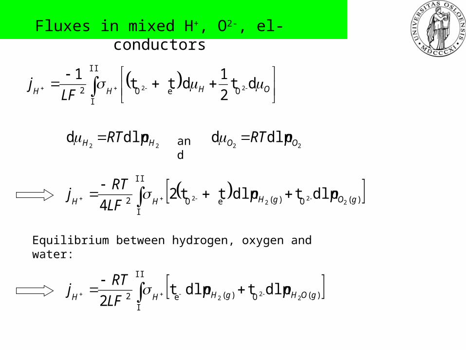
II

IOeO2

dt2

1d t t

1-2--2 OHHH LF

j

Fluxes in mixed H+, O2-, el-conductors

Equilibrium between hydrogen, oxygen and water:

22dlnd OO pRT

22dlnd HH pRT and

II

I

)(O)(eO2 2-2

2--2 dlntdln t t2

4 gOgHHHpp

LF

RTj

II

I

)(O)(e2 2-2

2- dlntdln t

2 gOHgHHHpp

LF

RTj

Fluxes in mixed H+, O2-, el-conductor

II

I

)(H)(eH2 22-22 dlnt2dln t t

8 gHgOOOpp

LF

RTj

Equilibrium between hydrogen, oxygen and water:

II

I

)(H)(e2 22-22 dlnt2dln t

8 gOHgOOOpp

LF

RTj

Ambipolar proton-electron conduction

II

I

)(O)(eO2 2-2

2--2 dlntdln t t2

4 gOgHHHpp

LF

RTj

Assume: 0t -2O

II

I

)(e2 2- dlnt

2 gHHHp

LF

RTj

Need to know how the proton conductivity and the electron transport number vary with in order to integrate the expression.)(2 gHp


Examples of partial pressure dependencies with varying defect situations

I2/1)(

II2/1)(2

0,II

I

)(2/1

)(2

0,

II

I

)(2/1

)(2

0,

2222

22

d2

dln2

gHgHH

gHgHH

gHgHH

H

ppLF

RTpp

LF

RT

ppLF

RTj

Assuming: Protons minority defects

Electronic transport no. ~1

II

I

)(4/3

)(2

0,

II

I

)(4/1

)(2

0,

22

22

d2

dln2

gHgHH

gHgHH

H

ppLF

RT

ppLF

RTj

Assuming: Protons majority defects,

compensated by electrons



II

I

)()(

2

II

I

)(2

2

2

2

d1

2

dln2

gHgH

H

gHH

H

ppLF

RT

pLF

RTj

Assuming: Protons majority defects, compensated by acceptor dopants



Proton concentration and conductivity independent of pH2

II

I

)(2

II

I

)(2

II

I

)(2

2

22

dln2

dln2

dln2

gHe

gHHegHeHH

pLF

RT

ptLF

RTpt

LF

RTj


If the transport number of protons ~1:

If protons charge compensate acceptors, the electronic conductivities have dependencies:

2/1)(2 gHe

p 2/1)(2

gHhp



II

I

)(2/1

)(2

0,

II

I

)(2/1

)(2

0,

22

22

d2

dln2

gHgHn

gHgHn

H

ppLF

RT

ppLF

RTj

Assuming: Protons majority defects, compensated by acceptors

Protonic transport no. ~1

Limiting n-type conductivity

II

I

)(2/3

)(2

0,

II

I

)(2/1

)(2

0,

22

22

d2

dln2

gHgHp

gHgHp

H

ppLF

RT

ppLF

RTj

Assuming: Protons majority defects, compensated by acceptors

Protonic transport no. ~1

Limiting p-type conductivity

Ambipolar proton-oxygen ion conduction

If the material is a mixed proton-oxygen ion conductor with negligible electronic transport number:

II

I

)(H2

II

I

)(O2 22

2-2 dlnt

2dlnt

2 gOHOgOHHHp

LF

RTp

LF

RTj

Water vapor

pressure ~ driving force

If material is acceptor doped, and protons or oxygen vacancies can be majority (compensating) defects:

If vO¨ compensating: 2/1

)(2 gOHHp

If H˙ compensating: 1

)(22

gOHOp

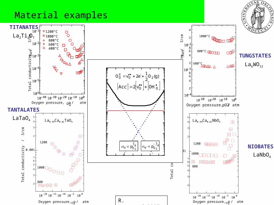
TITANATES

TUNGSTATES

NIOBATES

TANTALATES

10-6

10-5

10-4

10-3

10-2

10-1T

ota

l co

ndu

ctiv

ity,

tot /

S

/cm

10-40 10-30 10-20 10-10 100

Oxygen pressure, pO2 / atm

1200°C 1000°C 800°C 600°C 400°C

To

tal c

on

duct

ivity

/

S/c

m

2

3

4

5

6

7

0.001

2

3

4

5

10-20

10-15

10-10

10-5

100

La0.99Ca0.01NbO4

Oxygen pressure, pO 2 / atm

1200

800

1000

LaTaO4

LaNbO4

La6WO12

La2Ti2O7

Oxygen pressure, pO2 / atm

10-20

10-15

10-10

10-5

100

La0.99Ca0.01TaO4

To

tal c

on

duct

ivity

/

S/c

m

2

3

4

5

67

0.001

2

3

4

5

1200

1000

800

2

4

68

2

4

68

2

4

10-30 10-20 10-10 100

Oxygen pressure, / atm pO2

600°C

800°C

1000°C

To

tal c

on

duct

ivity

,

to

t /

S

/cm

10-2

10-4

10-3

41

Oh 2p 4

1

Oe 2p

)g(O2

1e2vO 2O

XO

OO OHv2cAc

Material examples

R. Haugsrud,2007

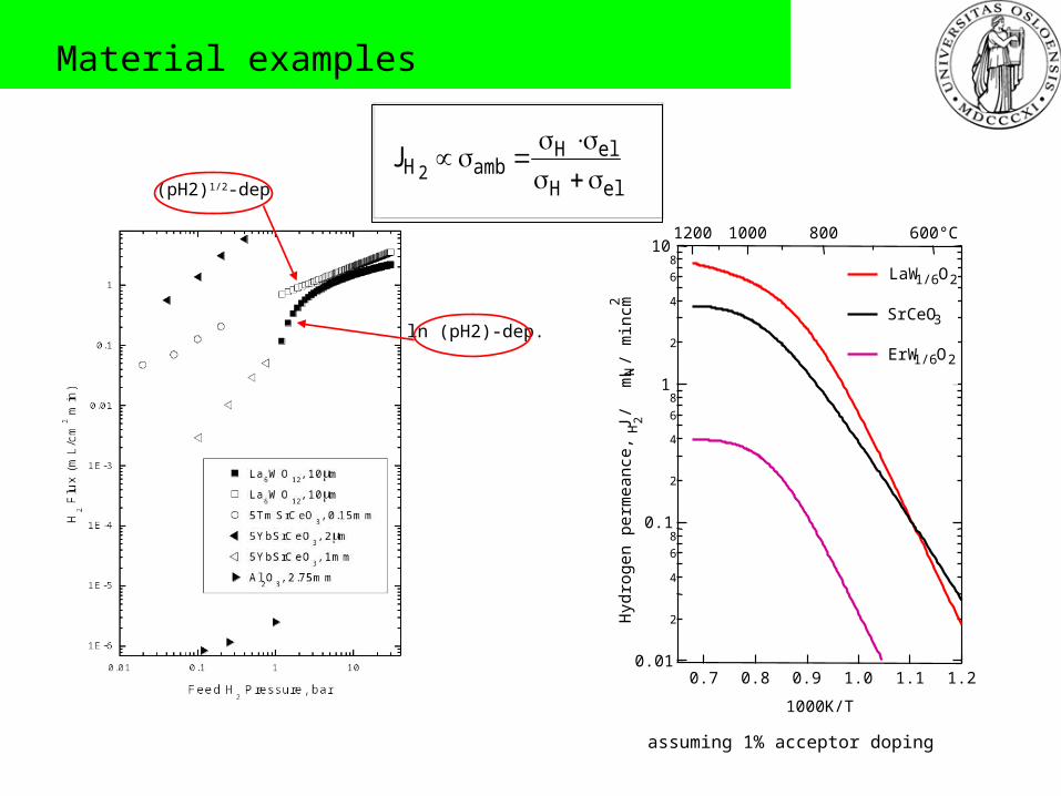
elH

elHambH2

J

0.01

2

4

6

80.1

2

4

6

81

2

4

6

810

Hyd

roge

n pe

rmea

nce,

JH

2 /

mL

N /

min

cm2

1.21.11.00.90.80.7

1000K/T

1200 1000 800 600°C

LaW1/6O2

SrCeO3

ErW1/6O2

assuming 1% acceptor doping

Material examples

(pH2)1/2-dep

ln (pH2)-dep.

10-5

10-4

10-3

10-2

Con

duct

ivity

,

/ S

/cm

1.81.61.41.21.00.8

1000K/T

1000 800 600 400°C

tot

H

O

el

ramp(10 kHz)

Material examples

Partial conductivities modeled under reducing conditions

La6WO12

k

ktot

Protons dominate until ~ 800 °C

All conductivities rise with rising T, until ~ 800 °C

Total conductivity rise with rising T

,2O e

increase in entire T-window

We have a small T-region where 2O dominates

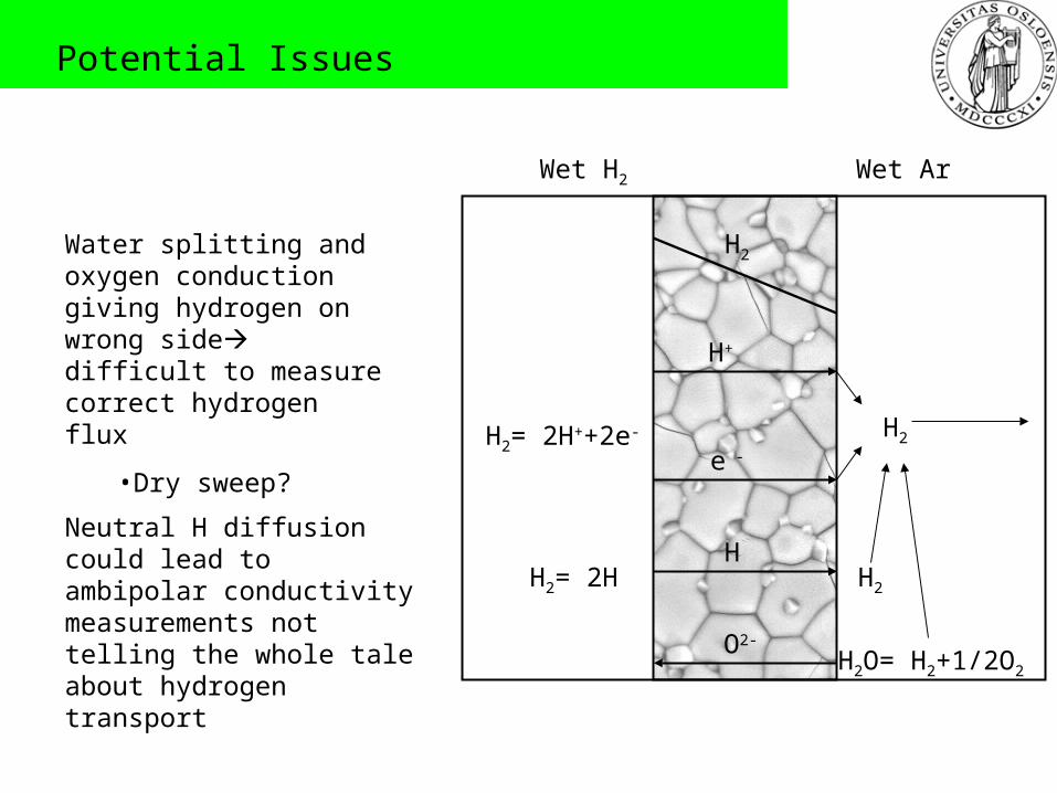
Potential Issues

Neutral H diffusion could lead to ambipolar conductivity measurements not telling the whole tale about hydrogen transport

Wet H2 Wet Ar

H2

H+

e -H2= 2H++2e- H2

H2O= H2+1/2O2

O2-

Water splitting and oxygen conduction giving hydrogen on wrong side difficult to measure correct hydrogen flux

•Dry sweep?

H2= 2HH

H2

II

I

)(e2 2- dlnt

2 gHHHp

LF

RTj

Potential Issues

What if the electronic transport number is dependent on oxygen partial pressure gradients?

How do we integrate the expression for the flux density in such a case?

II

I

)(e

1)(1

II

I

)(e)(1

II

I

)(e 2-

22-

22- dtdlntdlnt gH

XgHgH

XgHgHHH

ppKppKpKj

Integration by parts over a beer, anyone?

Sources

Norby, T. and Haugsrud, R., 2007, Membrane Technology Vol. 2: Membranes for energy conversion, Weinheim: WILEY-VCH

Kofstad, P. and Norby. T, 2006, Defects and transport in crystalline solids, University of Oslo

Haugsrud, R. 2007, New High-Temperature Proton Conductors (HTPC)-Applications in Future Energy Technology, New Materials for Membranes, GKSS

Serra, E., Bini, A.C., Cosoli, G. and Pilloni, L., 2005, Journal of the American Ceramic Society, 88, 15-18

Cheng, S., Gupta, V.K. and Lin, J.Y.S., 2005, Solid State Ionics, 176, 2653-2663

Hamakawa, S., Li, L., Li, A. and Iglesia, E., 2002, Solid State Ionics, 148, 71-83

skjalg erdal 1 dept. of chemistry, centre for materials science and nanotechnology,

Documents