sizing & allocation of pv units in distribution systems
TRANSCRIPT

Sizing & Allocation of PV Units in
Distribution Systems
by
Ameena Alsumaiti
A thesis
presented to the University of Waterloo
in fulfillment of the
thesis requirement for the degree of
Master of Applied Science
in
Electrical and Computer Engineering
Waterloo, Ontario, Canada, 2010
© Ameena Alsumaiti 2010

ii
AUTHOR'S DECLARATION
I hereby declare that I am the sole author of this thesis. This is a true copy of the thesis, including any
required final revisions, as accepted by my examiners.
I understand that my thesis may be made electronically available to the public.
iii
Abstract
The thesis focuses on allocation and sizing of PV units targeting the minimization of total cost of
electricity purchase from the grid taking in consideration the capital cost of the units. The PV sizing
and allocation problem is formulated as a mixed integer non linear programming (MINLP) problem
where the objective is to supply local loads and if excess generation is available, the PV system
would sell electricity back to the grid. The study is performed on the 13 bus radial feeder. The
allocation and sizing problem of PV units is performed following two approaches. In the first
approach, the problem is studied under demand-supply balance; while in the second approach, the
problem is investigated under AC power balance.
Since claims about PV units’ payback time exist in practice, this thesis considers a different strategy
based on which it would calculate the PV units payback time. It considers the capacity factor of PV
units that represents a percentage of PV output power depending on the availability of solar radiation.
The proposed problem formulation in this work can become a good tool for both utility and
customers. For utilities, the model proposed can provide an insight on the price of electricity that
should be paid for green PV energy. From a customer’s perspective, the proposed model can provide
the customer with a more accurate estimate of the PV payback time since the model takes into
account the variability in PV as well as the fact that not all PV generation will be exported to the grid
at a given moment. It would set the prices at which the customer would sell electricity to the grid at
certain age of PV units and would investigate the PV operation period at which the system would
consider their availability to be an advantage at the current PV electricity selling price as available in
the market.
Finally, the model presented in the study can be adapted to fit any region in the world taking into
account two major factors, the electricity market price in the area and the capacity factor of PV units.

iv
Acknowledgements
I praise and glorify Allah who creates a vicegerent on earth and who knows what I do not know.
Thanks goes to Allah giving me strength and support during the master degree journey.
I am heartily thankful to my home country United Arab Emirates and its rulers for their continuous
encouragement and support. My deepest gratitude goes to Sheikh Mohammed Bin Zayed Al Nahayan
for inspiration.
I would like to thank Masdar for my master scholarship and especially Dr. Sultan Aljaber for his
belief on Masdar students’ capabilities in research and development. My thanks go also to Dr.
Marwan Khraisheh, Dr. Yossef Shatilla and all Masdar Institute of Science and Technology staff.
I would like to express my sincere gratitude to my supervisors Professor Mehrdad Kazerani and
Professor Hatem Zeineldien for their endless encouragement and invaluable guidance throughout this
journey. My appreciation is also extended to Professor Magdy Salama for his encouragement.
I have been lucky enough to be raised in a loved family. Life without my parents would not be the
same. I would like to dedicate flowers: The first flower is a red rose and goes for my mother; the
second flower is a purple flower and is dedicated to my father. Gladiolus flowers are dedicated to my
beloved brother Abdulla and my uncle Hussein, yellow roses to my sisters and brothers and a lily to
me. Since flowers cannot be green, I would like to dedicate a white flower to my brother Faisal who
passed away before my graduation.
My deepest thanks go to my best friend in Waterloo, Zainab Meraj for her care and support. I cannot
imagine how life would be without her friendship.
To my colleagues, I would like to thank them for their advice and continuous encouragement.
Lastly, my regards go to all of those who supported me in any respect during the completion of my
thesis.
v
Dedication
To His Highness Sheikh Mohammed Bin Zayed Al-Nahayan
With my greatest gratitude
vi
Table of Contents
AUTHOR'S DECLARATION ............................................................................................................... ii
Abstract ................................................................................................................................................. iii
Acknowledgements ............................................................................................................................... iv
Dedication .............................................................................................................................................. v
Table of Contents .................................................................................................................................. vi
List of Figures ....................................................................................................................................... ix
List of Tables ......................................................................................................................................... x
Chapter 1 Introduction ........................................................................................................................... 1
1.1 Thesis Objective ........................................................................................................................... 1
1.2 Thesis Outline .............................................................................................................................. 2
Chapter 2 Distribution Generation & Renewable Energy Sources ........................................................ 3
2.1 Definition ..................................................................................................................................... 3
2.2 National Eras in the Development of Electricity Generation ....................................................... 3
2.3 Distribution Generation Resources .............................................................................................. 4
2.4 Distribution generation Capacity ................................................................................................. 5
2.5 Advantages of DG and Regulations ............................................................................................. 6
2.5.1 Electricity Market Liberalization & Flexibility Factor ......................................................... 7
2.5.2 Power Quality ....................................................................................................................... 8
2.5.3 DGs Advantage to the Grid ................................................................................................... 8
2.5.4 DGs & Environment ............................................................................................................. 9
2.5.5 Energy Security ................................................................................................................... 11
2.5.6 Points to Consider while Dealing with DGs ....................................................................... 12
2.5.7 Cost ..................................................................................................................................... 13
Chapter 3 Photovoltaic System ............................................................................................................ 14
3.1 Motivation to Use PV ................................................................................................................ 14
3.2 PV History ................................................................................................................................. 16
3.3 PV Cell ....................................................................................................................................... 18
3.4 PV Materials .............................................................................................................................. 18
3.4.1 Mono-Crystalline Silicon .................................................................................................... 18
3.4.2 Poly-Crystalline Silicon ...................................................................................................... 19
3.4.3 Amorphous Silicon ............................................................................................................. 19
vii
3.4.5 Industrial Perspective toward PV Material .......................................................................... 19
3.5 PV Configuration ....................................................................................................................... 20
3.6 PV System Classes ..................................................................................................................... 22
3.6.1 Stand Alone PV System ...................................................................................................... 22
3.6.2 Grid Connected PV System ................................................................................................. 22
3.7 Solar Radiation Characteristics .................................................................................................. 23
3.8 Previous Studies on optimal Size and Location of RES ............................................................. 24
Chapter 4 Sizing & Allocation of PV units in Distribution systems Optimization Problem Definition
.............................................................................................................................................................. 29
4.1 Objectives ................................................................................................................................... 29
4.2 Optimal Power Flow .................................................................................................................. 29
4.3 Type of Optimization Problem to be solved ............................................................................... 30
4.4 Selected Software ....................................................................................................................... 30
4.5 Optimization Problem ................................................................................................................ 30
4.6 Estimated Market Price .............................................................................................................. 31
4.7 PV Output Power ........................................................................................................................ 33
4.8 Chapter 4 Summary .................................................................................................................... 36
Chapter 5 Optimal Sizing & Location of PV Units under Demand-Supply Balance without Feeder
Power Flow Representation .................................................................................................................. 37
5.1 Problem Definition & Optimization Problem Formulation ........................................................ 37
5.1.1 Objective Function .............................................................................................................. 37
5.1.2 Equality Constraints ............................................................................................................ 38
5.1.3 Inequality Constraints .......................................................................................................... 39
5.2 13 bus Feeder Case Study........................................................................................................... 40
5.2.1 Substation Transformer ....................................................................................................... 41
5.2.2 Load ..................................................................................................................................... 41
5.3 Results based on Demand-Supply Balance without Feeder Power Flow Representation for13
Bus Radial Feeder ............................................................................................................................ 43
5.3.1 Objective Function With Respect to PV Operation Period ................................................. 44
5.3.2 Allocation and Sizing of PV Units ...................................................................................... 45
5.3.3 Capital Cost Reduction over Years under Demand-Supply Balance without Feeder Power
Flow Representation ..................................................................................................................... 48
viii
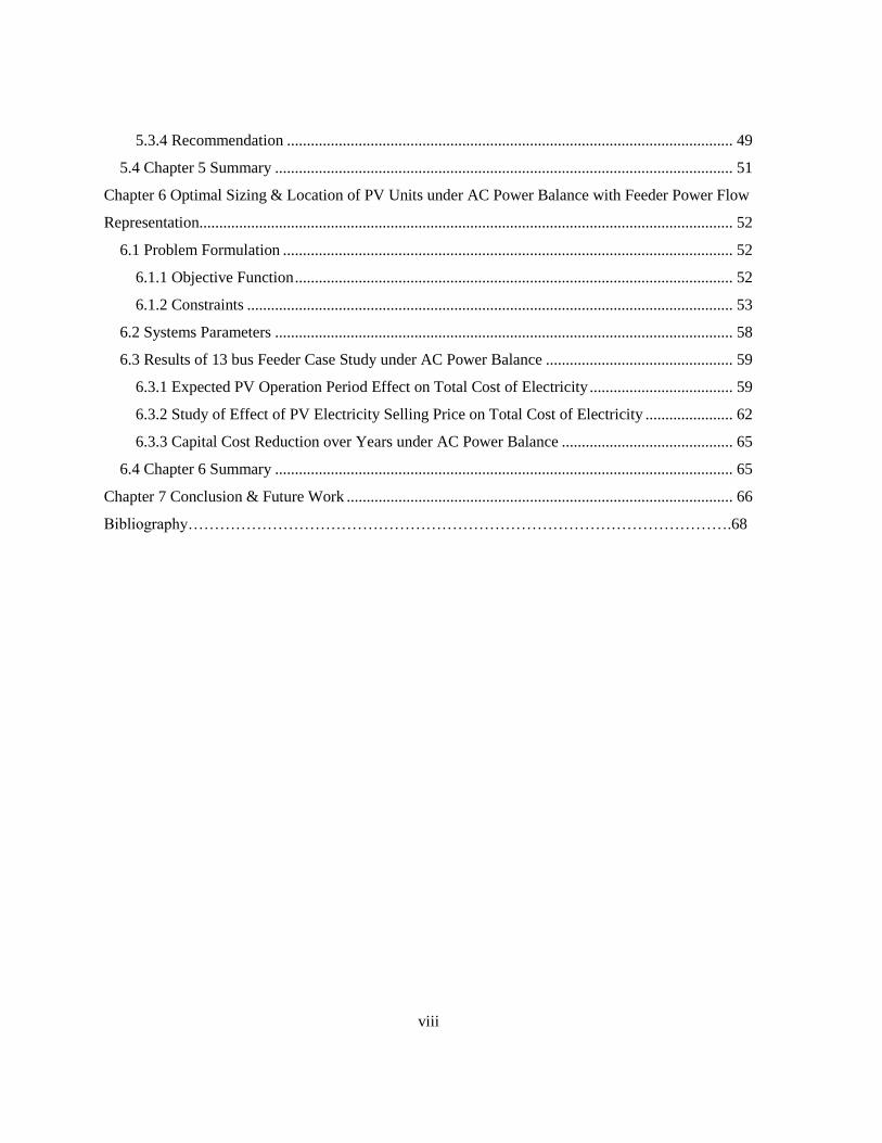
5.3.4 Recommendation ................................................................................................................ 49
5.4 Chapter 5 Summary ................................................................................................................... 51
Chapter 6 Optimal Sizing & Location of PV Units under AC Power Balance with Feeder Power Flow
Representation...................................................................................................................................... 52
6.1 Problem Formulation ................................................................................................................. 52
6.1.1 Objective Function .............................................................................................................. 52
6.1.2 Constraints .......................................................................................................................... 53
6.2 Systems Parameters ................................................................................................................... 58
6.3 Results of 13 bus Feeder Case Study under AC Power Balance ............................................... 59
6.3.1 Expected PV Operation Period Effect on Total Cost of Electricity .................................... 59
6.3.2 Study of Effect of PV Electricity Selling Price on Total Cost of Electricity ...................... 62
6.3.3 Capital Cost Reduction over Years under AC Power Balance ........................................... 65
6.4 Chapter 6 Summary ................................................................................................................... 65
Chapter 7 Conclusion & Future Work ................................................................................................. 66
Bibliography………………………………………………………………………………………….68
ix
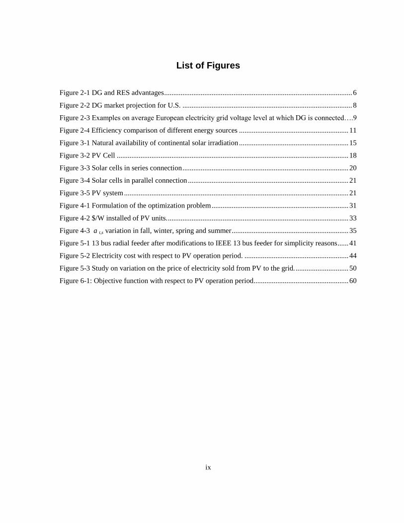
List of Figures
Figure 2-1 DG and RES advantages ....................................................................................................... 6
Figure 2-2 DG market projection for U.S. ............................................................................................. 8
Figure 2-3 Examples on average European electricity grid voltage level at which DG is connected….9
Figure 2-4 Efficiency comparison of different energy sources ............................................................ 11
Figure 3-1 Natural availability of continental solar irradiation ............................................................ 15
Figure 3-2 PV Cell ............................................................................................................................... 18
Figure 3-3 Solar cells in series connection ........................................................................................... 20
Figure 3-4 Solar cells in parallel connection ........................................................................................ 21
Figure 3-5 PV system ........................................................................................................................... 21
Figure 4-1 Formulation of the optimization problem ........................................................................... 31
Figure 4-2 $/W installed of PV units. ................................................................................................... 33
Figure 4-3 a t,s variation in fall, winter, spring and summer ................................................................ 35
Figure 5-1 13 bus radial feeder after modifications to IEEE 13 bus feeder for simplicity reasons ...... 41
Figure 5-2 Electricity cost with respect to PV operation period. ......................................................... 44
Figure 5-3 Study on variation on the price of electricity sold from PV to the grid. ............................. 50
Figure 6-1: Objective function with respect to PV operation period .................................................... 60
x
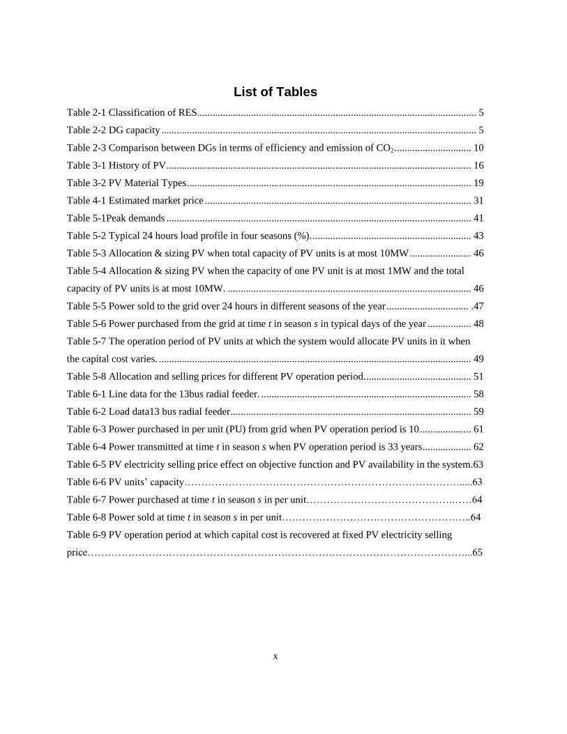
List of Tables
Table 2-1 Classification of RES............................................................................................................. 5
Table 2-2 DG capacity ........................................................................................................................... 5
Table 2-3 Comparison between DGs in terms of efficiency and emission of CO2 .............................. 10
Table 3-1 History of PV ....................................................................................................................... 16
Table 3-2 PV Material Types ............................................................................................................... 19
Table 4-1 Estimated market price ........................................................................................................ 31
Table 5-1Peak demands ....................................................................................................................... 41
Table 5-2 Typical 24 hours load profile in four seasons (%). .............................................................. 43
Table 5-3 Allocation & sizing PV when total capacity of PV units is at most 10MW ........................ 46
Table 5-4 Allocation & sizing PV when the capacity of one PV unit is at most 1MW and the total
capacity of PV units is at most 10MW. ............................................................................................... 46
Table 5-5 Power sold to the grid over 24 hours in different seasons of the year ................................ .47
Table 5-6 Power purchased from the grid at time t in season s in typical days of the year ................. 48
Table 5-7 The operation period of PV units at which the system would allocate PV units in it when
the capital cost varies. .......................................................................................................................... 49
Table 5-8 Allocation and selling prices for different PV operation period. ......................................... 51
Table 6-1 Line data for the 13bus radial feeder. .................................................................................. 58
Table 6-2 Load data13 bus radial feeder .............................................................................................. 59
Table 6-3 Power purchased in per unit (PU) from grid when PV operation period is 10 .................... 61
Table 6-4 Power transmitted at time t in season s when PV operation period is 33 years ................... 62
Table 6-5 PV electricity selling price effect on objective function and PV availability in the system.63
Table 6-6 PV units’ capacity……………………………………………………………………….....63
Table 6-7 Power purchased at time t in season s in per unit…………………………………….……64
Table 6-8 Power sold at time t in season s in per unit………………………………………………..64
Table 6-9 PV operation period at which capital cost is recovered at fixed PV electricity selling
price…………………………………………………………………………………………………...65

1
Chapter 1
Introduction Distribution Generation (DG) and Renewable Energy Sources (RES) have attracted the attention of
different countries in the world. The term distributed generation can be defined as the local generation
of electricity that can be associated with heat generation in a cogeneration system. Different
terminologies can be used to refer to distributed generation. These are on site generation, dispersed
generation, embedded generation, decentralized generation or decentralized energy.
The distribution generation technology is developing very fast in many countries as its resources
provide clean energy. Abu Dhabi City located in UAE has a bold vision to transform itself to a global
leader in the field of sustainable energy. Masdar city is a global cooperative platform initiated by the
city of Abu Dhabi in order to determine solutions for energy security, climate change and sustainable
human development. It has been chosen as the headquarters for International Renewable Energy
Agency.
Solar cells become an attractive option of renewable energy sources when considering the climate of
the country. This thesis targets the selection of optimal sizes and locations of the PV units in the city
by minimizing the total cost of electricity purchase from the grid plus the PV capital cost minus the
electricity sold to the grid, but since the city is under establishment, the study is performed on a 13
bus radial feeder that is originally adapted from IEEE 13 bus feeder but with certain modifications
made to the system.
The domain of this thesis is in the field of modeling and analysis. The optimization problem is solved
using mixed integer non linear programming. The problem is solved taking into account power
balance constraints, total power loss, voltage limits, transmission line limits, PV unit’s capacity and
its initial cost limits.
1.1 Thesis Objective There are two important factors that determine the payback time of PV units which are the PV capital
cost, the electricity price as well as the PV capacity factor. Thus, the main objective of this thesis is
twofold:
1. To determine the payback time of PV units taking into account PV output variation.
2. To determine the utility electricity price at which the PV payback time would be reasonable.

2
1.2 Thesis Outline The proposed work is interesting as it is a suggestion for a real application on a city under
establishment. The thesis is organized as follows:
Chapter 2 provides the reader with an overview of distribution generation and renewable energy
resources. It presents the advantages of distribution generation.
Chapter 3 introduces photovoltics that is the selected distributed generation class to be used and
shows the availability of solar energy over the world. It presents Abu Dhabi vision toward sustainable
renewable energy reflected into Masdar city. Moreover, it describes the photovoltaic system and the
materials used to manufacture solar cells.
Chapter 4 starts with introducing the objective of the thesis that is to determine the optimal size and
location of PV units in different distribution systems under demand-supply balance and AC power
balance. It presents the software used ―GAMS‖ as a simulation tool for the studies. It also presents the
data to be integrated with the system under study to achieve the target of the thesis and considers the
first type of study which is to allocate the PV units and size them under demand-supply balance.
It discusses the optimization problem and the models needed.
Chapter 5 is focused on finding the optimal size and location of PV units under demand-supply
balance. It presents the optimization problem formulation for this type of study and discusses the
determined results. Moreover, the recommendation is also presented for this study.
Chapter 6 considers the problem of sizing and allocation of PV units under AC power balance and
provides the reader with the results and recommendation. Chapter 7 summarizes the project and suggests future work.
3
Chapter 2
Distribution Generation & Renewable Energy Sources The distribution generation technology is developing very fast in many countries as its renewable
resources provide clean energy. This chapter defines distribution generation. It presents its advantages
and provides the reader with an overview of renewable energy sources.
2.1 Definition Distribution Generation (DG) can be defined as electricity generation at small scale to satisfy the
demands close to the load being supplied at distribution level voltage [1],[ 2]. There is no common
agreed definition on DG. The installation and operation of electric power generation units that are
connected to the network on the customer side of meter are recognized as distribution generation [3].
CIRED identified five factors behind the increased interest in DG. These are reduced gaseous
emissions, completion policy deregulation, variety of energy sources, the efficiency of energy or
logical use of energy and the requirement of national power [4]. CIGRE added to these factors the
following: presence of modular plant for generation, locations for smaller generators that are to be
found easily, the length of the construction period that is to be short and the capital costs of smaller
plants that should be low. Generation may be sited closer to load resulting in a reduction in the
transmission costs [5].
Building new transmission lines in an energy plant would be expensive. This problem can be avoided
through the investment in DG. Since there are a variety of energy sources and a reliable grid is
targeted, DG is considered as an attractive option. DG is considered to be a flexible technology as it is
capable of meeting peak demands of power. Such flexibility is coupled with load profile, cost,
reliability and availability of energy as power supply might be needed to be uninterrupted. The
environment is a major concern as carbon emission results in pollution. Such factors define the
reasons behind the increased interest in DG based on the definition of International Energy Agency
(IEA) [2], [6], [7].
2.2 National Eras in the Development of Electricity Generation Central station plants have been in use to generate electric power as a matter of economics of scale [8]. The first main power plant was opened by George Westinghouse in Niagra Falls in 1895
by using alternating current [9].
4
Some of electricity customers mostly in the industrial field decided to run their own power generator
considering the economical perspective. Besides that, facilities such as hospitals and
telecommunication sectors use their own power generators during power outage. These power
generators were under the control of the customers rather than the utilities, which made it
advantageous in overall as customers are supplied with their demands especially when operating
away from the grid rather than purchasing electricity from the local electricity provider or when it is
not possible to supply the customers operating away from it. Under the first circumstance, it is
possible to expand the electricity network as the electricity to be generated to supply such customers
is not utilized and it can be redirected to the network to be invested [10].
The utility has decided to switch from the economics of scale to what is called mass production [11].
In 1970s and 1980s, the system of electricity in some countries was developed to be hybrid including
both centralized and distributed generation units as environmental concerns started to arise because of
the availability of natural gas for power generation [12]. Based on [9], 2% of the energy in the U.S
was involved in producing electricity in 1920; while today the percentage is much more above that.
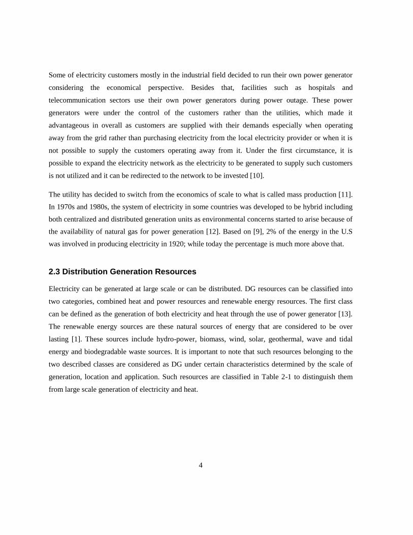
2.3 Distribution Generation Resources Electricity can be generated at large scale or can be distributed. DG resources can be classified into
two categories, combined heat and power resources and renewable energy resources. The first class
can be defined as the generation of both electricity and heat through the use of power generator [13].
The renewable energy sources are these natural sources of energy that are considered to be over
lasting [1]. These sources include hydro-power, biomass, wind, solar, geothermal, wave and tidal
energy and biodegradable waste sources. It is important to note that such resources belonging to the
two described classes are considered as DG under certain characteristics determined by the scale of
generation, location and application. Such resources are classified in Table 2-1 to distinguish them
from large scale generation of electricity and heat.
5
Table 2-1 Classification of RES
Generation Combined heat &power Characteristic Renewable energy source Characteristic
Large Scale
Generation.
Large district heating
>50MW
Scale Large hydro
>10MW
Scale
Large industrial combined
heat and power >50MW
Application &
scale
Offshore wind Location
Co-firing biomass in coal
power plant
Application
Geothermal energy Scale
DG Medium district heating Scale Medium & small hydro Scale
Medium industrial combined
heat and power
Scale &
application
Onshore wind Location
Commercial combined heat
and power
Application Tidal energy Scale
Micro combined heat and
power
Scale Biomass and waste
incineration/gasification
Scale &
application
Solar energy Scale
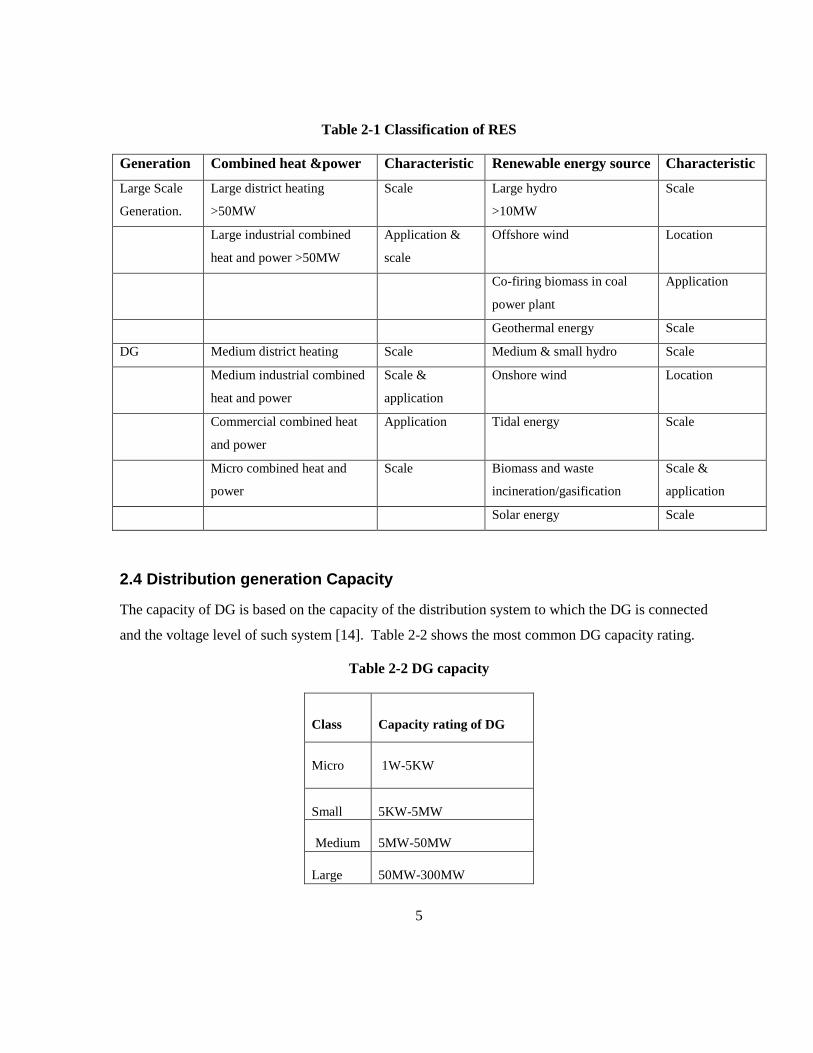
2.4 Distribution generation Capacity
The capacity of DG is based on the capacity of the distribution system to which the DG is connected
and the voltage level of such system [14]. Table 2-2 shows the most common DG capacity rating.
Table 2-2 DG capacity
Class
Capacity rating of DG
Micro
1W-5KW
Small
5KW-5MW
Medium
5MW-50MW
Large
50MW-300MW
6
The energy supplied by DG is either consumed within the distribution system or fed back to the
transmission system if the energy produced is greater than what the load in a distribution system
requires [14].
2.5 Advantages of DG and Regulations Distribution generation is a term that includes a variety of technologies, including many renewable
technologies, combined heat and power plants , back-up and peak load systems. These technologies
provide many advantages including new market opportunities and improved competitiveness in the
industrial sector [6].
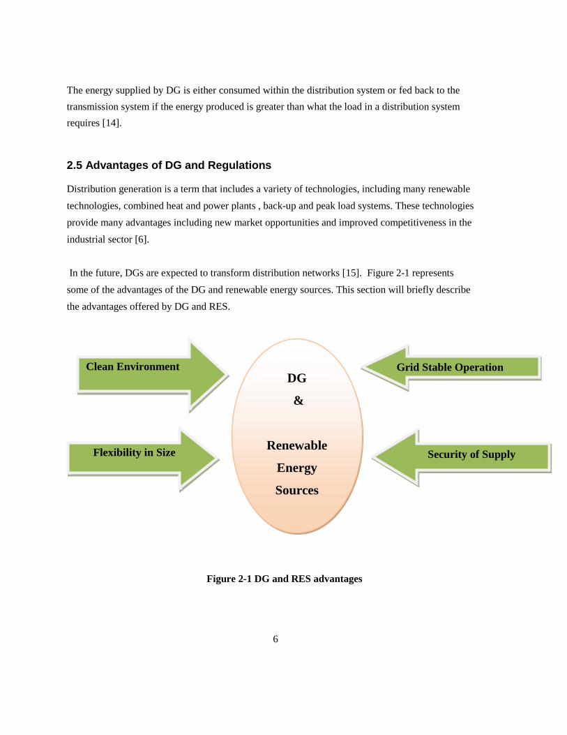
In the future, DGs are expected to transform distribution networks [15]. Figure 2-1 represents
some of the advantages of the DG and renewable energy sources. This section will briefly describe
the advantages offered by DG and RES.
Figure 2-1 DG and RES advantages
Flexibility in Size
Clean Environment DG
&
Renewable
Energy
Sources
Grid Stable Operation
Security of Supply
7
2.5.1 Electricity Market Liberalization & Flexibility Factor DG permits the players in the electricity sector to respond in a flexible manner to the changes in the
conditions of the market. The flexibility of the technologies of DG results from their small sizes and
the short construction lead times when compared to the large power plants that are centralized [12].
Since DG technologies are flexible in their size and operation, and they can be expanded easily, they
play a major role in reacting to electricity price fluctuations. For instance, heat applications in Europe
drive the need for DG in the market; while in US, the volatility of price drives the demand for DG
[12]. Distributed generation had been developed for the reason of improving the overall fuel
efficiency of the power plant.
The demand for DGs is controlled by price volatility. DGs can either operate continuously or for
specific periods within the day. The schedule of operation of DG technologies is dependent on the
demand of electricity and thermal energy. Furthermore, fuel prices and utility rates contribute to the
operation of DGs. When a DG is selected to operate continuously, it would operate for 8760 hours per
year in order to supply a continuous power to the demand. This time excludes, the time needed for its
maintenance. On the other hand, if the DG is chosen to be operating for part of the day, then it is
responsible for the supply of an intermediate power. Intermediate power can be defined as the power
generated during the schedule of operation of DG. To decide on the operating schedule of the DG, the
difference between the cost of electricity generation and electricity purchasing from the utility should
be determined. If the cost of generation is less than the cost of purchasing by the utility, then DG is to
operate; otherwise it will not operate [14].
Based on option value theory, [16] and [17] recommend the operation of flexible power plants during
the peak periods as this is to be more profitable when compared to the conventional evaluations’
option.
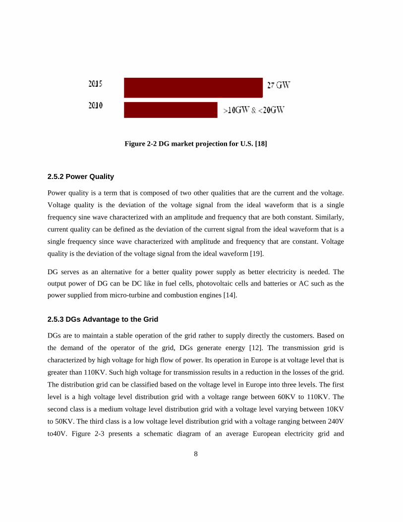
A long term market offer for DG at small scale in U.S and worldwide is projected by Gas Research
Institute (GRI). Certain issues resembled in the restructuring of the utility would result in uncertainty
in the market that would provide a limit on the market penetration. The projection made by GRI for
U.S expects the power to be 27GW with a capital equipment purchase of $10 billion by the year 2015
as shown in Figure 2-2 [18].
8
Figure 2-2 DG market projection for U.S. [18]
2.5.2 Power Quality Power quality is a term that is composed of two other qualities that are the current and the voltage.
Voltage quality is the deviation of the voltage signal from the ideal waveform that is a single
frequency sine wave characterized with an amplitude and frequency that are both constant. Similarly,
current quality can be defined as the deviation of the current signal from the ideal waveform that is a
single frequency since wave characterized with amplitude and frequency that are constant. Voltage
quality is the deviation of the voltage signal from the ideal waveform [19].
DG serves as an alternative for a better quality power supply as better electricity is needed. The
output power of DG can be DC like in fuel cells, photovoltaic cells and batteries or AC such as the
power supplied from micro-turbine and combustion engines [14].
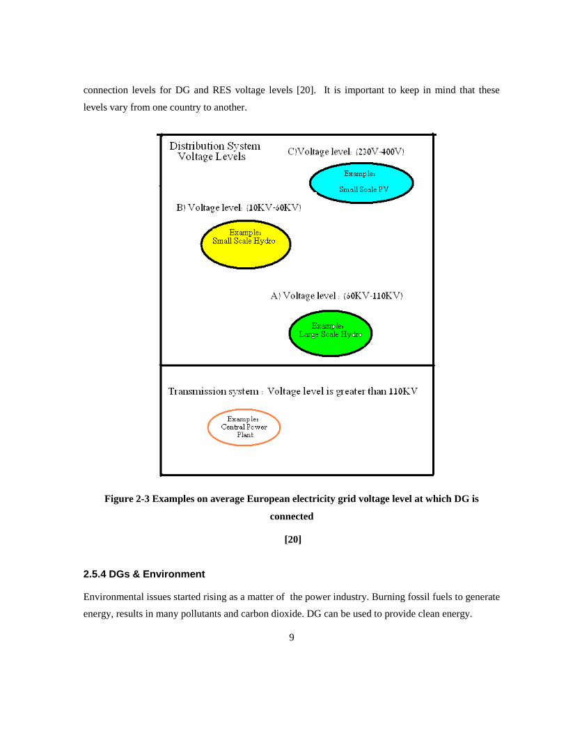
2.5.3 DGs Advantage to the Grid DGs are to maintain a stable operation of the grid rather to supply directly the customers. Based on
the demand of the operator of the grid, DGs generate energy [12]. The transmission grid is
characterized by high voltage for high flow of power. Its operation in Europe is at voltage level that is
greater than 110KV. Such high voltage for transmission results in a reduction in the losses of the grid.
The distribution grid can be classified based on the voltage level in Europe into three levels. The first
level is a high voltage level distribution grid with a voltage range between 60KV to 110KV. The
second class is a medium voltage level distribution grid with a voltage level varying between 10KV
to 50KV. The third class is a low voltage level distribution grid with a voltage ranging between 240V
to40V. Figure 2-3 presents a schematic diagram of an average European electricity grid and
9
connection levels for DG and RES voltage levels [20]. It is important to keep in mind that these
levels vary from one country to another.
Figure 2-3 Examples on average European electricity grid voltage level at which DG is
connected
[20]
2.5.4 DGs & Environment Environmental issues started rising as a matter of the power industry. Burning fossil fuels to generate
energy, results in many pollutants and carbon dioxide. DG can be used to provide clean energy.

10
Combined heat and power generation can be used for applications where heat and electricity are both
in demand rather than using an external boiler to deliver heat and purchasing electricity from the grid.
The DG market is partially driven by the availability of more efficient, more cost-effective
distribution technologies. CHP conserves energy by 10% to 30% based on the size and consequently
the efficiency of cogeneration units. Moreover, through the installation of DG units, it is possible to
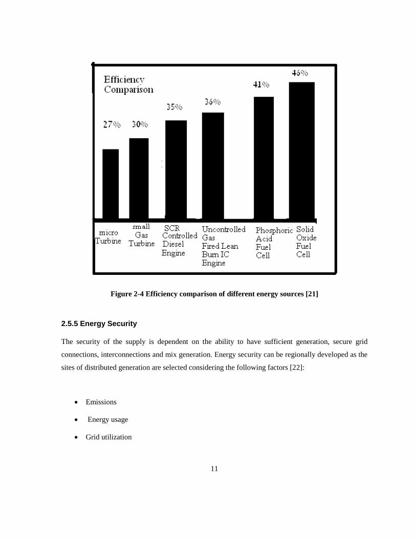
use cheap fuel [12]. Table 2-3 and Figure 2-4 provide an example on a comparison case between two
distribution generators different energy sources both DGs and centralized generation in terms of
efficiency and emission [21]. Such comparison is made on the basis of lb/MWh. A higher efficient
system is recognized for producing less pollution per MWh [21].
Table 2-3 Comparison between DGs in terms of efficiency and emission of CO2 [21]
Comparison Uncontrolled
gas fired
lean burn IC
engine
SCR
controlled
diesel
generator
Solid
oxide
fuel cell
Phosphoric
acid fuel
cell
Micro-
turbine
Gas
turbine
(small)
CO2
(LB/MWh)
1099
1537
867
937
1477
1329
Efficiency
(Btu/KWh)
9402
9646
7420
8324
12641
11374
11
Figure 2-4 Efficiency comparison of different energy sources [21]
2.5.5 Energy Security
The security of the supply is dependent on the ability to have sufficient generation, secure grid
connections, interconnections and mix generation. Energy security can be regionally developed as the
sites of distributed generation are selected considering the following factors [22]:
Emissions
Energy usage
Grid utilization

12
Since the demand and the use of natural gas as a primary source of energy increases, the security of
energy decreases. On the other hand, there is a case in which the security of energy is enhanced as
efficiency of the fuel is high and its consumption is low. This case is CHP in which both heat and
power are generated. The increased penetration of both renewable energy sources and DGs with a
high efficiency in terms of energy results in a secure supply through a reduction in the energy imports
and the establishment of a diverse portfolio of energy [12],[23].
2.5.6 Points to Consider while Dealing with DGs
There are certain points to be considered while dealing with DGs such as operating frequency of the
system, voltage profile, reactive power, power conditioning and system protection. Frequency
deviation is encountered when DG is connected to the system and this deviation should be kept as low
as possible to achieve the right performance of the system by careful planning of DG installation. DG
can cause instability problems on voltage profile as a matter of bi-directional power flow of the
current that makes it difficult to tune protection schemes. When DGs at small and medium sizes are
used, they may not produce reactive power as they use asynchronous generators. This problem can be
solved by having a DG unit with a power electronic interface for certain reactive power production.
In terms of power conditioning, PV and fuel cells as examples of DGs are capable of DC production.
As a result, a DC/AC inverter is needed to connect them to the grid which results in harmonics [12].
Specific control techniques can be applied to control the injection of these harmonics [14].
The increase in the rate of electricity as well as the rates of standby and backup in areas that are
served by utility, result in off grid application which is the most economical mean for electricity
production for remote areas with high load factors [24].
In off grid applications, the site is disconnected from the electric grid. In such applications, DG units
are responsible for continuous generation with backup capabilities onsite. In addition, usually utilities
assess DG operators with capacity charges that are dependent on the size of the DG system. Utility
charges different rates for both energy and demand when the DG system is down [24].

13
2.5.7 Cost
From an investment point of view, it is most likely to be much easier to locate RES and DG compared
to large central power plant. Furthermore, the time needed to have DG units on the site is shorter than
what will be spent in constructing in a power plant.
The capital cost for installing a DG is high when compared to large central plants. The capital cost
differs from one DG technology to another. For example, the capital cost for combustion turbine is
$1292.24 US/ KW; while it is $25848 US/KW for fuel cells [2].
DGs can reduce the transmission and distribution losses as well as the transmission and distribution
costs. As the customer size is smaller, the sharing price of the transmission and distribution in the
electricity cost is larger. This is greater than 40% for households [2]. Using DG results in a reduction
in the losses of the grid by 6.8% and this will contribute to 10% to 15% saving of the cost [2], [25].
As a matter of the vital role that renewable energy plays in the reduction of CO2, such reduction in
gaseous emission is reflected into cost. Moreover, Jobs have been created as a matter of the
investments carried out in the field of renewable energy.
14
Chapter 3
Photovoltaic System
Photovoltaic (PV) system can be defined as an energy system that converts the solar energy into
electricity through the use of semiconductor materials compromising PV cells. The PV cells are
connected together in different combinations that can be series, parallel or both to form PV arrays.
They might be integrated with storage banks to save the excess generated energy or to act as a battery
back up to supply electricity when needed. PV systems can be classified into two classes based on
the application they are used for. The first class is the grid connected PV system; while the second
class is the stand alone PV system. The following sections will provide a brief description of the
materials used to design PV and will describe the differences between the two PV systems [26].
Moreover, it presents the different classes of storage system and the selected storage system to be
involved in this thesis.
3.1 Motivation to Use PV
The economy of United Arab Emirates had been dependent on crude oil and gas exports as the main
source of national income. Its reserve of crude oil is 9.5%; while the reserve of natural gas is 3.5%
[27].
United Arab Emirates is located in region where solar energy is widely available, which makes solar
energy an attractive option to be invested to raise the national income while maintain sustainability
and clean environment. The sustainability is defined by the integration of economy, society and
environment Abu Dhabi city, the capital of United Arab Emirates, occupies 80% of the country land
with 30% of the total population. The city sets a long term vision to be not reliant on fossil fuel and to
maintain a safe environment [27].
When selecting a renewable energy resource, certain requirements should be studied in advance.
These are limits in the efficiency, size of the plant, structural restrictions that is considered to be
essential in case of PV such that the availability of suitable areas or competitive uses is studied, and
reliability of energy supply, and space requirements. When considering solar energy, it can be noted

15
that the natural availability of continental solar irradiation is extraordinary huge as represented by the
largest cube in Figure 3-1 [28].
Figure 3-1 Natural availability of continental solar irradiation [28]
The world wide has been attracted by solar technologies as solar energy is sustainable. Masdar
initiative at Abu Dhabi is adopting solar technologies in United Arab Emirates. Photovoltaics and
concentrating solar power projects are developing in Abu Dhabi such that Masdar is provided with
broad coverage of the solar sector [29].
16
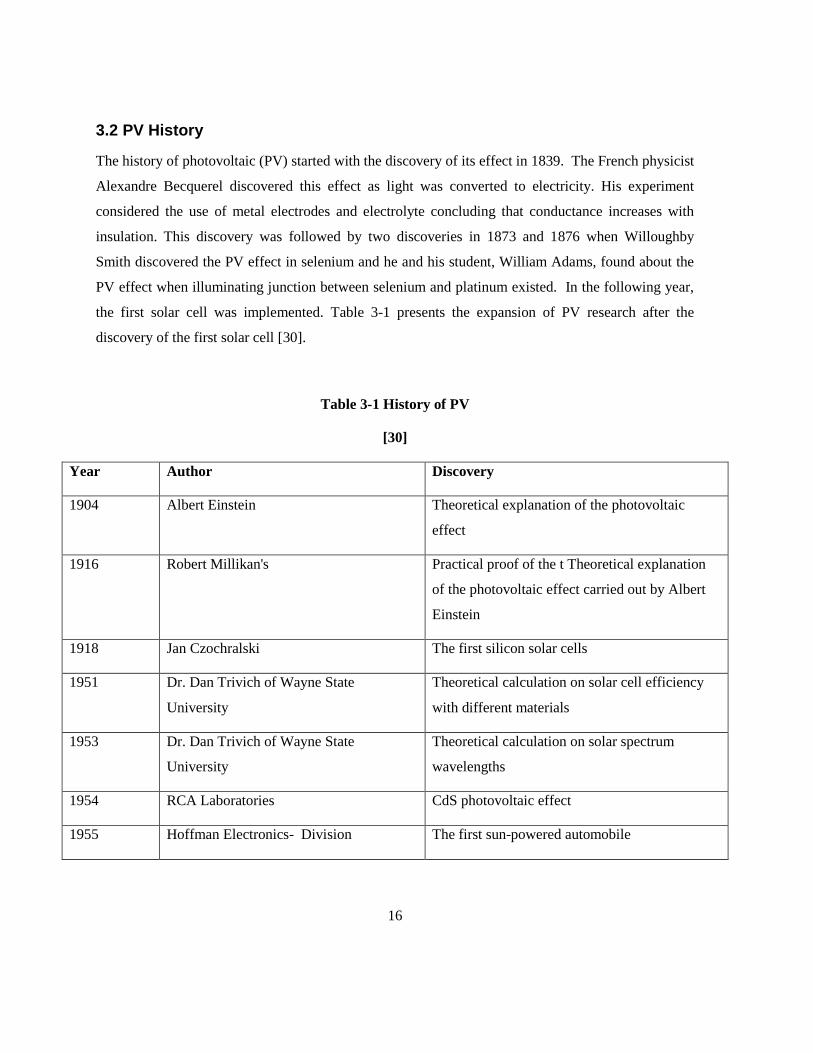
3.2 PV History
The history of photovoltaic (PV) started with the discovery of its effect in 1839. The French physicist
Alexandre Becquerel discovered this effect as light was converted to electricity. His experiment
considered the use of metal electrodes and electrolyte concluding that conductance increases with
insulation. This discovery was followed by two discoveries in 1873 and 1876 when Willoughby
Smith discovered the PV effect in selenium and he and his student, William Adams, found about the
PV effect when illuminating junction between selenium and platinum existed. In the following year,
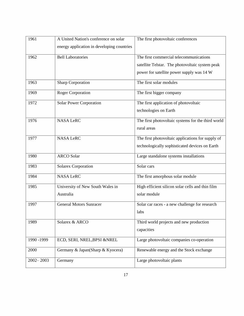
the first solar cell was implemented. Table 3-1 presents the expansion of PV research after the
discovery of the first solar cell [30].
Table 3-1 History of PV
[30]
Year Author Discovery
1904 Albert Einstein Theoretical explanation of the photovoltaic
effect
1916 Robert Millikan's Practical proof of the t Theoretical explanation
of the photovoltaic effect carried out by Albert
Einstein
1918 Jan Czochralski The first silicon solar cells
1951 Dr. Dan Trivich of Wayne State
University
Theoretical calculation on solar cell efficiency
with different materials
1953 Dr. Dan Trivich of Wayne State
University
Theoretical calculation on solar spectrum
wavelengths
1954 RCA Laboratories CdS photovoltaic effect
1955 Hoffman Electronics- Division The first sun-powered automobile
17
1961 A United Nation's conference on solar
energy application in developing countries
The first photovoltaic conferences
1962 Bell Laboratories The first commercial telecommunications
satellite Telstar. The photovoltaic system peak
power for satellite power supply was 14 W
1963 Sharp Corporation The first solar modules
1969 Roger Corporation The first bigger company
1972 Solar Power Corporation The first application of photovoltaic
technologies on Earth
1976 NASA LeRC The first photovoltaic systems for the third world
rural areas
1977 NASA LeRC The first photovoltaic applications for supply of
technologically sophisticated devices on Earth
1980 ARCO Solar Large standalone systems installations
1983 Solarex Corporation Solar cars
1984 NASA LeRC The first amorphous solar module
1985 University of New South Wales in
Australia
High efficient silicon solar cells and thin film
solar module
1997 General Motors Sunracer Solar car races - a new challenge for research
labs
1989 Solarex & ARCO Third world projects and new production
capacities
1990 -1999 ECD, SERI, NREL,BPSI &NREL Large photovoltaic companies co-operation
2000 Germany & Japan(Sharp & Kyocera) Renewable energy and the Stock exchange
2002– 2003 Germany Large photovoltaic plants
18
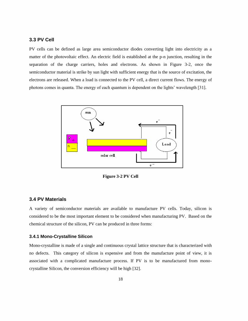
3.3 PV Cell
PV cells can be defined as large area semiconductor diodes converting light into electricity as a
matter of the photovoltaic effect. An electric field is established at the p-n junction, resulting in the
separation of the charge carriers, holes and electrons. As shown in Figure 3-2, once the
semiconductor material is strike by sun light with sufficient energy that is the source of excitation, the
electrons are released. When a load is connected to the PV cell, a direct current flows. The energy of
photons comes in quanta. The energy of each quantum is dependent on the lights’ wavelength [31].
Figure 3-2 PV Cell
3.4 PV Materials
A variety of semiconductor materials are available to manufacture PV cells. Today, silicon is
considered to be the most important element to be considered when manufacturing PV. Based on the
chemical structure of the silicon, PV can be produced in three forms:
3.4.1 Mono-Crystalline Silicon
Mono-crystalline is made of a single and continuous crystal lattice structure that is characterized with
no defects. This category of silicon is expensive and from the manufacture point of view, it is
associated with a complicated manufacture process. If PV is to be manufactured from mono-
crystalline Silicon, the conversion efficiency will be high [32].

19
3.4.2 Poly-Crystalline Silicon
Polycrystalline Silicon is composed from many silicon crystals that are small in size. This category
of silicon has been used in the MOSFET and CMOS industry since a long time because of its
conducting characteristic. Polycrystalline silicon is recognized for showing greater stability when
exposed to electric field and light induced stress. Polycrystalline silicon has the advantage of being
simpler and cheaper comparing to mono-crystalline silicon; however, its grain boundaries between
the crystalline in silicon cell results in a lower efficiency [32].
3.4.3 Amorphous Silicon
Amorphous silicon has lower efficiency compared to mono-crystalline and poly-crystalline silicon. It
is characterized to have a low cost and low efficiency [33].
3.4.4 Industrial Perspective toward PV Material
The main differences between the different classes of PV materials in terms of efficiency, cost and
power per area are presented in Table 3.2 [33].
Table 3-2PV Material Types
[33]
Solar module
material type
Efficiency of
solar module
Cost of
solar
module
Power Area of
solar module
A) Mono -
crystalline
solar module
Varies
between 10%
to 13%
High cost High power
area
B) Poly -
crystalline
solar module
Varies
between 9%
to 13%
Moderate
cost
Moderate
power area
C)Amorphous
solar module
Varies
between 6% to
8%
Low cost Low power area
20
From the industrial point of view presented in an article in renewable energy access in [34], the
industry should focus on utilizing multi-crystalline silicon rather than mono-crystalline silicon even
though the latter shows better performance because of the lower cost of the first class of materials.
The production cost of mono-crystalline silicon is less than the multi-crystalline one which would be
reflected into saving from the economical perspective.
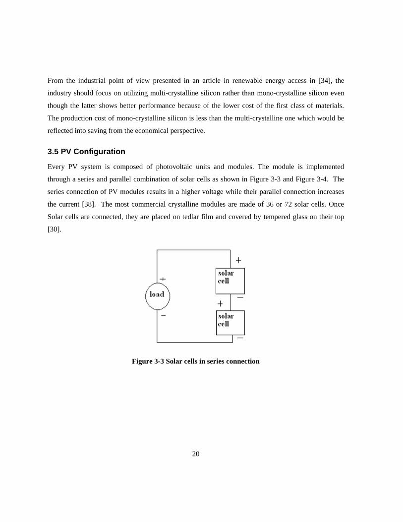
3.5 PV Configuration
Every PV system is composed of photovoltaic units and modules. The module is implemented
through a series and parallel combination of solar cells as shown in Figure 3-3 and Figure 3-4. The
series connection of PV modules results in a higher voltage while their parallel connection increases
the current [38]. The most commercial crystalline modules are made of 36 or 72 solar cells. Once
Solar cells are connected, they are placed on tedlar film and covered by tempered glass on their top
[30].
Figure 3-3 Solar cells in series connection
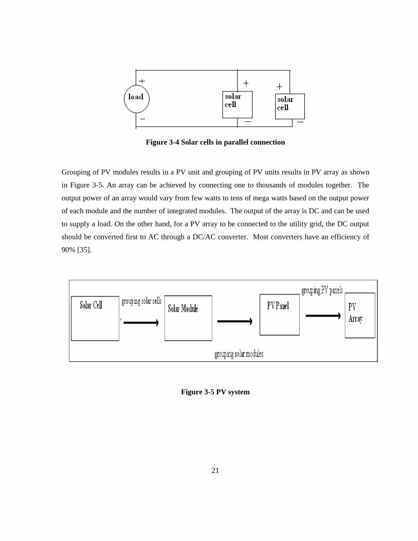
21
Figure 3-4 Solar cells in parallel connection
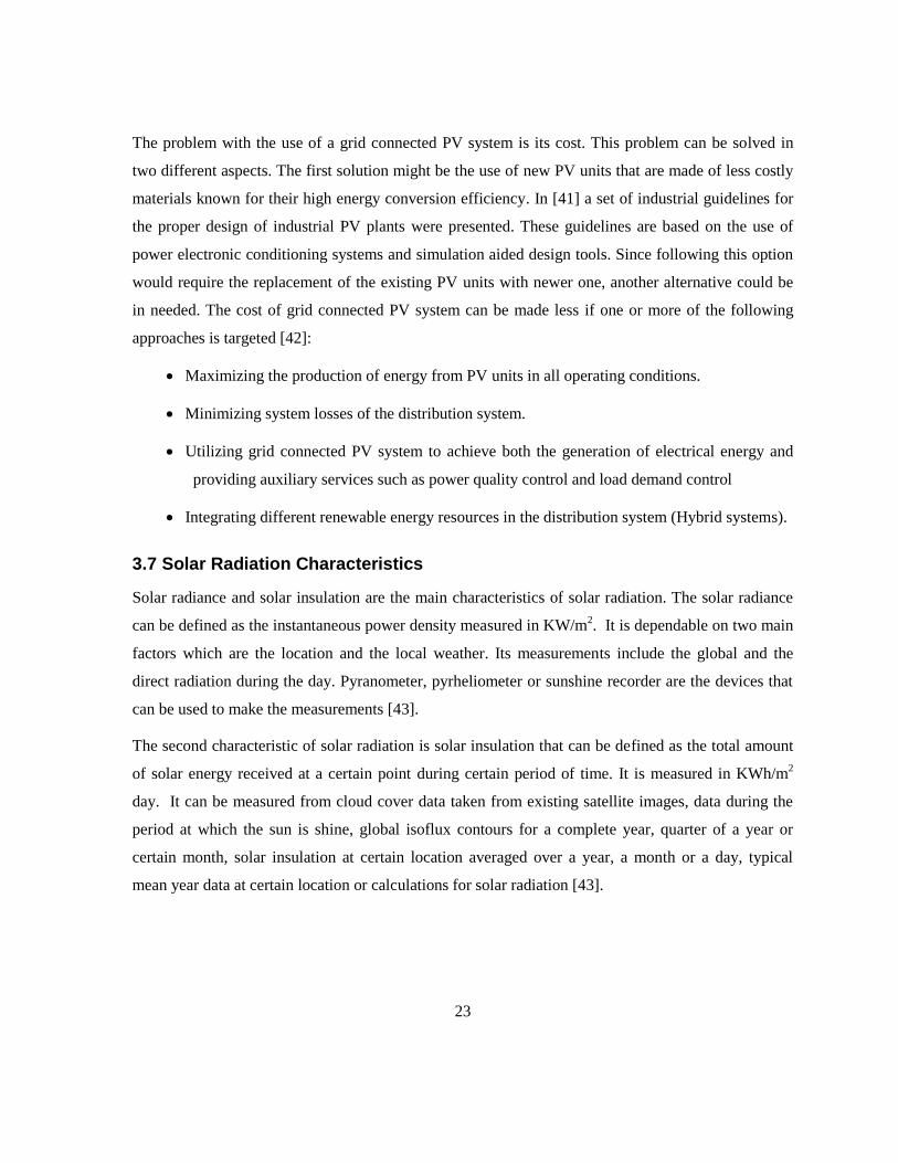
Grouping of PV modules results in a PV unit and grouping of PV units results in PV array as shown
in Figure 3-5. An array can be achieved by connecting one to thousands of modules together. The
output power of an array would vary from few watts to tens of mega watts based on the output power
of each module and the number of integrated modules. The output of the array is DC and can be used
to supply a load. On the other hand, for a PV array to be connected to the utility grid, the DC output
should be converted first to AC through a DC/AC converter. Most converters have an efficiency of
90% [35].
Figure 3-5 PV system

22
PV system might be integrated with storage banks to save the excess generated energy or to act as a
battery back up to supply electricity when needed
3.6 PV System Classes
PV systems can be classified into two classes based on the application they are used for. The first
class is the grid connected PV system; while the second class is the stand alone PV system. The
following section will describe the differences between the two systems [26].
3.6.1 Stand Alone PV System
Stand alone PV system is capable of supplying the load with power when they are off grid connected.
This might take place when there is a fault in the distribution system. Such system is often integrated
with back up batteries storing solar energy during the day time to be used at night or when needed
[26].
From the economical point of view, this system could be used to supply remote areas as it becomes an
attractive option when considering how cost effective it is when comparing this cost to the cost of
connecting the load with other utility line extensions [36],[37],[38].
Various research have been carried out to optimize the energy systems. For example, [39] proposes a
model to optimize the PV array and storage bank for a stand-alone hybrid wind/PV system taking into
account the long term hourly solar insulation level data and the peak load demand data for the
selected site. The study presents the number of PV arrays to be used; however, it does not show the
influence of such system on the hybrid system cost. Later on, the authors in [39] expanded their study
to include the cost of the PV modules and storage bank [40].
3.6.2 Grid Connected PV System
Grid connected PV system is recognized as the latest technology of PV systems. This system is
capable to supplement the electricity supplied by the utility company. When the energy level
generated by a grid connected PV system is greater than the load level of the customer, the difference
in energy can be transferred to the utility. As a matter, the meter of the customer will be turned
backward and that would be reflected on the total cost of electricity to be paid by the customer. On
the other hand, when the condition that the energy generated from PVs is not enough to meet the
demands of the customer, electricity will be purchased from the utility company [26].
23
The problem with the use of a grid connected PV system is its cost. This problem can be solved in
two different aspects. The first solution might be the use of new PV units that are made of less costly
materials known for their high energy conversion efficiency. In [41] a set of industrial guidelines for
the proper design of industrial PV plants were presented. These guidelines are based on the use of
power electronic conditioning systems and simulation aided design tools. Since following this option
would require the replacement of the existing PV units with newer one, another alternative could be
in needed. The cost of grid connected PV system can be made less if one or more of the following
approaches is targeted [42]:
Maximizing the production of energy from PV units in all operating conditions.
Minimizing system losses of the distribution system.
Utilizing grid connected PV system to achieve both the generation of electrical energy and
providing auxiliary services such as power quality control and load demand control
Integrating different renewable energy resources in the distribution system (Hybrid systems).
3.7 Solar Radiation Characteristics
Solar radiance and solar insulation are the main characteristics of solar radiation. The solar radiance
can be defined as the instantaneous power density measured in KW/m2. It is dependable on two main
factors which are the location and the local weather. Its measurements include the global and the
direct radiation during the day. Pyranometer, pyrheliometer or sunshine recorder are the devices that
can be used to make the measurements [43].
The second characteristic of solar radiation is solar insulation that can be defined as the total amount
of solar energy received at a certain point during certain period of time. It is measured in KWh/m2
day. It can be measured from cloud cover data taken from existing satellite images, data during the
period at which the sun is shine, global isoflux contours for a complete year, quarter of a year or
certain month, solar insulation at certain location averaged over a year, a month or a day, typical
mean year data at certain location or calculations for solar radiation [43].
24
3.8 Previous Studies on optimal Size and Location of RES
In [44], an iterative scheme to find the mix of wind-PV system with a storage system is presented.
The optimal size is determined based on the calculated values of life cycle unit cost of power
generation or relative excess power generated or unutilized energy probability for a certain deficiency
of power supply probability. The authors in [45] apply genetic algorithm to allocate DG in order to
reduce losses and improve voltage profile. In [46], the excess capacity of a system composed on PV,
wind, hydro and diesel is optimized. Strategic placement of distribution generation capacity is
described in [47]. In [48], a heuristic approach is presented to optimize the investment by determining
the optimal site and size of DG under the assumption that the DG size is a multiple of a provided
capacity. In [49], a method to determine the optimal location and size of PV grid connected systems
in distribution systems is presented. The problem was formulated as multi-objective function
involving strategies to evaluate both the technical impact associated with improving the stability of
the voltage of the feeder and the economical effect associated with the increase of loading limits is
used.
Particle swarm optimization algorithm is proposed in [50] in order to allocate three type of DG by
minimizing the losses in the system. The location and size of DG is randomly generated. The particle
keeps moving from its recent position considering the distance from its local point with a velocity
until reaching the global point. The results prove that particle swarm optimization would lead to
better results when it is compared to heuristic search technique [50].
Genetic algorithm and tabu search are applied in a new technique to determine the optimal location of
dispersed generation is distribution systems. In this algorithm, losses in distribution systems have
been reduced when compared to losses in genetic algorithm [51].
The allocation and sizing problem of DG is considered in [52] to minimize system losses. The
algorithm followed is tabu search and system losses are determined when DGs are allocated in the
system. Numerical simulation has been conducted in order to check the validity of the algorithm.
The optimization problem that targets the allocation and sizing of the distribution generators in
distribution system presented in [53] is focused on minimizing system losses taking into
consideration, the variability of the load with respect to voltage and frequency. The algorithm
followed is genetic algorithm. The loads in the study are considered to be fixed and varying. It has

25
been found that the location of distributed generator is independent on the load model, but the
objective function and the size of distributed generator affects by the load model. The variation in the
frequency affected the losses of the system and the size of distributed generator. The voltage has
improved in the system as a matter of the presence of distributed generator.
A combination of genetic algorithm and simulated annealing for optimal DG allocation in distribution
networks is considered in [54]. The problem focuses on minimizing system losses at fixed number of
DGs and specific total capacity. This study shows the effectiveness of the proposed mixed algorithm
when compared to SGA.
The optimal location of DG that is operating at optimal power factor is determined in [55]. The study
follows an analytical method in order to find the location of DG and it places the DG at busses with
highest suitability index. The study recommends operating DG at 0.8 unit factor as in order to achieve
a better performance of the system. This improvement is in terms of system losses reduction and
voltage profile improvement.
In [56], the optimal location and of distribution generators is determined applying bee colony
optimization that is a member of swarm intelligence, while considering a multiple objective function
that is to minimize the real power loss and violation function of contingency analysis. The major
constraints are the power generation limits and power balance. This study proves that less simulation
time can be reached applying bee colony optimization when compared to genetic algorithm, search
tabu and simulated annealing.
In [57], the allocation and sizing of distributed generators are achieved by focusing on minimizing the
distribution generators cost and maximizing the reliability at the same time. A major constraint in the
optimization problem is the active power balance between the distributed generators and the load
during the isolation time. Load shedding has been assumed in this study such that the active power of
distribution generators is in one zone separated from the fault in the system by sectionalizers is less
than total active power of the loads in that zone. Loads will be shed one by one applying the priority
maintaining the active power balance. Such consideration of load shedding would result in a smaller
reliability index if compared to the case that loads are shed when the power of distribution generators
becomes less than the total power of the loads.
The optimal allocation of DG is determined based on a cost/worth analysis. The study takes into
26
consideration both technical and economical factors which involve energy loss, load point, reliability
indices, cost of DG cost and DG’s portability. The optimization problem focuses on maximizing the
benefit to cost ratio of DG application. It has been found in this study that the number of DG
displacement to decrease when the benefit to cost ratio increases [58].
In [59], optimal power flow and genetic algorithm are considered in order to allocate certain number
of DGs in distribution network. The use of such combination would allow dynamic network operators
to search network for the optimal locations that permits strategic placement of small number of DGs
through a large number of potential combinations. The software implementing the suggested
algorithm is Matlab incorporating some features used in MATPOWER.
Genetic algorithm is applied in [60], in order to optimally allocate and size DGs by minimizing the
location charges for active power at the busses in the distribution system. This is achieved by using
various voltage dependent static load models. Nodal pricing and per unit location charges that are
involved in short term operation of transmission systems can be applied also in distribution systems.
The simulation is carried out on radial feeder and networked system involving one DG and many of
them. A major constraint in the optimization problem is that the voltage should not be violated at all
the busses. The results of this study show that the location of DG does not change irrespective of
different load models; however, the size of DG is affected by the models of load. As the load
exponent increases, there is decay in the objective function until it reaches the minimum. Further
increase in the load exponent would lead the objective function to increase. In networked systems, the
influence of the load exponent is found to be marginal when compared to radial distribution. This is
due to small variation in the voltage in such systems in networked systems. If radial distribution
system is considered, then the allocation of many DGs in the system would results decrease the
objective function compared to distribution system involving only one DG. The availability of more
than one DG in the network would improve the objective function by reducing the average location
charges at the busses without violating the voltage constraints.
There is no common agreement on the payback time of PV units. The payback time of PV units can
be defined in terms of energy and cost. If the payback time is defined in terms of energy, it would
mean the time needed to recover the inserted energy to manufacture PV units such that the PV units
can output the corresponding power [61]. The other definition is based on cost and that is associated
with the recovery of PV cost through selling energy to the grid. The Feed in Tariff is the price at
27
which the PV output power would be sold at to the grid. This price is set by Ontario’s government in
such a way to incentivize consumers to use PV units. By doing so, the government can achieve two
main objectives which are increased energy efficiency and increased renewable energy penetration.
The difference between the optimal payback time calculated in the work and the payback life time
presented in [61] and [62] is that this thesis targets the supplement of system demands from the power
generated from PV units such that the electricity purchase from the grid is minimized taking into
consideration the capital cost of PV units. Moreover, it adds to previous research by considering the
variability of solar radiation over the 24 hours of the year. This is implemented by defining a capacity
factor which is the ratio of PV output power to the PV rated capacity.
From previous research, it can be noted that most of the research targeted the allocation and sizing of
distributed generators based on system losses minimization. Some of them performed cost/worth
analysis. Different optimization methods had been followed. Comparing to previous studies, this
work is focused on optimal allocation and size of certain distributed generation units that are PV
units. The work considers a 13 bus radial distribution feeder. Two approaches have been followed in
order to allocate and size PV units in the systems. These are the demand-supply balance without
feeder power flow representation and the AC power balance with the representation of feeder power
flow. The problem in the first approach is modeled as a mixed integer linear programming problem;
while in the second approach it is modeled as a mixed integer non linear programming problem. This
study determines the location and the size of PV units by minimizing the total cost of electricity
purchase from the grid plus the capital cost of PV units minus the electricity cost of selling energy
from PV units back to the grid. This study differs from previous studies in that it considers the
variability of the load being supplied, the capacity factor of PV units and the requirement to supply
the demand from PV units before selling any extra generated electricity from the PV units to the grid.
The work determines the location and size of PV units in the following way:
1. It determines the objective function behavior, the minimum total cost of electricity purchase from
the grid plus the cost of PV units minus the cost of electricity generated from PV and sold back to the
grid, over the expected operation period of PV units and finds the point at which it would be suitable
to allocate and size PV units in the system.
2. It finds the best electricity selling price of PV units for a selected operation period of PV units

28
based on which the PV units will be allocated and sized in the distribution system.
3. It investigates the effect of the variation of the capital cost of PV units on the allocation of PV units
in the system.
It is important to emphasize that the study assumes an average market price and neglects the discount
rate that could be a point to be investigated in the future to improve the study.
29
Chapter 4
Sizing & Allocation of PV units in Distribution systems
Optimization Problem Definition
4.1 Objectives
The thesis targets the optimal allocation and sizing of different PV units whose maximum capacities
are selected based on the number of busses in the distribution system selected. The location and the
size of PV units are determined by focusing on minimizing the total cost of electricity purchase from
the grid plus the capital cost of PV units net the cost of selling electricity generated from PV units
back to the grid. In this thesis, the system selected on which the problem is to be studied is13 bus
feeder that has been originally adapted from IEEE 13 bus radial feeder but after applying certain
modifications. The optimization problem formulated is tested by implementing two studies which
include:
Demand-supply balance without feeder power flow representation.
AC power balance with the representation of feeder power flow.
The second objective is to investigate the impact of variation in the cost of selling electricity from the
PV to the grid on the PV location and total cost.
4.2 Optimal Power Flow
During the last decade, optimal power flow literature has seen dramatic rise focusing on two points
that are the solution methodologies and the areas of application. Optimal power flow was defined in
1960s as an extension of the conventional economic load dispatch problem to find the optimal setting
for control variables satisfying power system constraints. The optimal power flow solution is
considered to be more accurate that the economic load dispatch solution. The optimal power flow
problem can have different objective functions depending on the nature of the problem selected. For
example, the objective can be minimizing transmission loss such as in reactive power planning area,
or can be minimizing the generation shift. The optimal power flow problem can involve different
control variables and system constraints depending on the requirement of the problem. These control
variables can involve [63]:
30
Active power generation
Reactive power generation
Switched capacitor setting
Active power of the load
Reactive power of the load
Transformer tap setting
4.3Type of Optimization Problem to be solved
The problem of allocating and sizing PV units is formulated as mixed integer linear programming
(MILP) under demand-supply balance without power flow representation and as a mixed integer non
linear programming problem (MINLP) under AC power balance with the representation of feeder
power flow. In a linear programming problem, the objective function and the constraints are linear.
An NLP problem can be defined as the process of finding a solution to a mathematical system that is
composed of equalities and inequalities recognized as constraints over unknown variables that are real
with an objective function to be maximized or minimized. For NLP problems, either the objective
function or the constraint is nonlinear. In mixed integer programming some or all the variables are
integers.
4.4 Selected Software
GAMS software is a general algebraic modeling system that has been chosen to be the simulation tool
for this work. This software is recognized for being a high level modeling system for optimization
problems. The software is associated with many solvers. CPLEX is used to solve the MIP problem;
while SBB is chosen to be the solver for the MINLP problem [64].
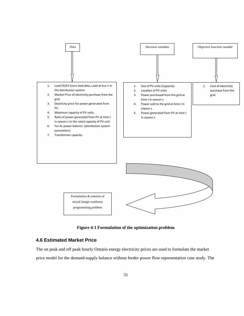
4.5 Optimization Problem
The optimization problem to be solved is made of an objective function subject to certain constraints.
The objective function, the decision variable and the data needed to optimally locate and size PV
units are summarized in Figure4-1.
31
Figure 4-1 Formulation of the optimization problem
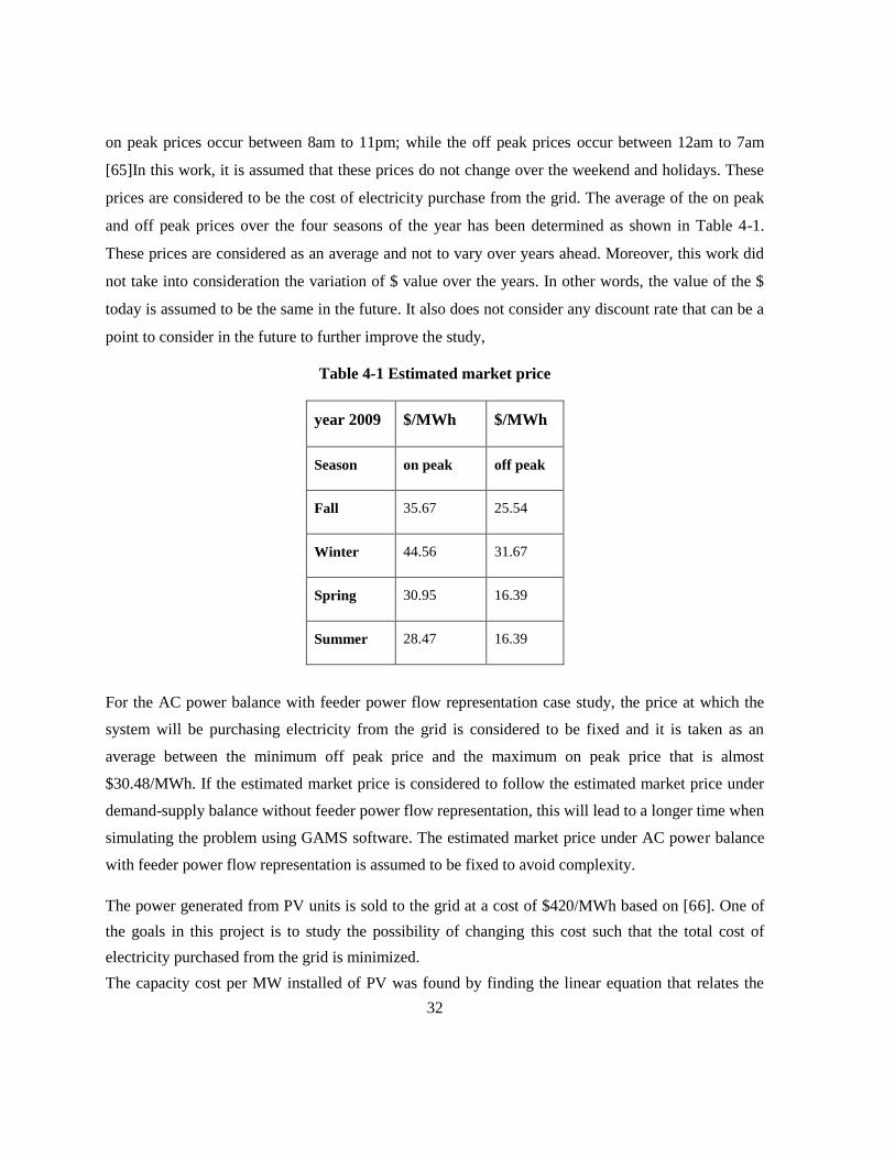
4.6 Estimated Market Price
The on peak and off peak hourly Ontario energy electricity prices are used to formulate the market price model for the demand-supply balance without feeder power flow representation case study. The
Formulation & solution of
mixed integer nonlinear
programming problem
1. Load (%)24 hours load data, Load at bus n in
the distribution system.
2. Market Price of electricity purchase from the
grid.
3. Electricity price for power generated from
PV.
4. Maximum capacity of PV units.
5. Ratio of power generated from PV at time t
in season s to the rated capacity of PV unit.
6. For Ac power balance: (distribution system
parameters)
7. Transformer capacity.
1. Size of PV units (Capacity)
2. Location of PV units
3. Power purchased from the gird at
time t in season s
4. Power sold to the grid at time t in
season s
5. Power generated from PV at time t
in season s
1. Cost of electricity
purchase from the
grid.
Data Decision variables Objective function variable
32
on peak prices occur between 8am to 11pm; while the off peak prices occur between 12am to 7am
[65]In this work, it is assumed that these prices do not change over the weekend and holidays. These
prices are considered to be the cost of electricity purchase from the grid. The average of the on peak
and off peak prices over the four seasons of the year has been determined as shown in Table 4-1.
These prices are considered as an average and not to vary over years ahead. Moreover, this work did
not take into consideration the variation of $ value over the years. In other words, the value of the $
today is assumed to be the same in the future. It also does not consider any discount rate that can be a
point to consider in the future to further improve the study,
Table 4-1 Estimated market price
year 2009 $/MWh $/MWh
Season on peak off peak
Fall 35.67 25.54
Winter 44.56 31.67
Spring 30.95 16.39
Summer 28.47 16.39
For the AC power balance with feeder power flow representation case study, the price at which the
system will be purchasing electricity from the grid is considered to be fixed and it is taken as an
average between the minimum off peak price and the maximum on peak price that is almost
$30.48/MWh. If the estimated market price is considered to follow the estimated market price under
demand-supply balance without feeder power flow representation, this will lead to a longer time when
simulating the problem using GAMS software. The estimated market price under AC power balance
with feeder power flow representation is assumed to be fixed to avoid complexity.
The power generated from PV units is sold to the grid at a cost of $420/MWh based on [66]. One of
the goals in this project is to study the possibility of changing this cost such that the total cost of
electricity purchased from the grid is minimized.
The capacity cost per MW installed of PV was found by finding the linear equation that relates the

33
cost in $ to the capacity of PV unit from BP company [67]. The relationship is plotted in Figure 4-
3and the linear factor is found to be $4000/KW.
Figure 4-2 $/W installed of PV units.
4.7 PV Output Power
The output power of PV to the rated capacity over 24 hours of the day is to be determined. With the
availability of global irradiance measurements in a typical day in different seasons, the output power
can be found applying equation (0-1):
ApowerotputPV (4-1) [68]
where
A: Area of PV unit
λ: Irradiance (W/m2)
η : Efficiency
η is the resultant from different efficiencies as shown in equation (4-2):
invMPPTlossDCmismatchdustrated
(4-2) [69]
Where

34
rated: Rated efficiency of PV module (10.77%).
dust : 1 - the fractional power loss due to dust and debris on the PV array (96%).
mismatch : 1- the fractional power loss due to module parameter mismatch (95%).
lossDC
: 1 - the DC-side I2R losses (98%).
MPPT : 1 - the power loss due to DC current ripple and "algorithm error" caused by the switching
converter which performs the maximum power point tracking function (95%).
inv: DC/AC inverter efficiency (97%)
The data for solar irradiance is obtained from the Solar Radiation Research Laboratory [70]. Since the
available capacity of PV, in this work, is 1MW, the area of the PV unit can be found as shown in
Table 4-2.
Table 4-2 Area of IMW PV
Area of 50W PV module [71]
839mm*537mm =0.450543m2
Area of 1MW
(1MW/50W)*Area of 50W PV module= 9010.86m2
The ratio between the PV output power and its rated capacity (1MW) in different seasons (at,s) has
been calculated applying (4-4) as shown in Table 4-3:
at,s = PV output power / Rated capacity of PV (4-3)
This variation is plotted in Figure 4-4. It can be concluded from this table that the maximum radiation
duration is in the summer season followed by spring, fall and winter.
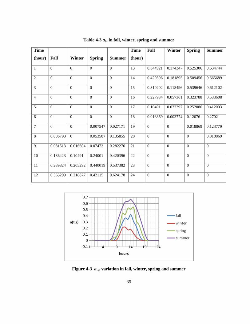
35
Table 4-3 at,s in fall, winter, spring and summer
Time
(hour) Fall Winter Spring Summer
Time
(hour)
Fall Winter Spring Summer
1 0 0 0 0 13 0.344921 0.174347 0.525306 0.634744
2 0 0 0 0 14 0.420396 0.181895 0.509456 0.665689
3 0 0 0 0 15 0.310202 0.118496 0.539646 0.612102
4 0 0 0 0 16 0.227934 0.057361 0.323788 0.533608
5 0 0 0 0 17 0.10491 0.023397 0.252086 0.412093
6 0 0 0 0 18 0.018869 0.003774 0.12076 0.2702
7 0 0 0.007547 0.027171 19 0 0 0.018869 0.123779
8 0.006793 0 0.053587 0.135855 20 0 0 0 0.018869
9 0.081513 0.016604 0.07472 0.282276 21 0 0 0 0
10 0.186423 0.10491 0.24001 0.420396 22 0 0 0 0
11 0.289824 0.205292 0.440019 0.537382 23 0 0 0 0
12 0.365299 0.218877 0.42115 0.624178 24 0 0 0 0
Figure 4-3 a t,s variation in fall, winter, spring and summer
36
4.8 Chapter 4 Summary
This chapter presented the type of optimization problem to be solved and the selected simulation tool.
The optimization problem under the demand-supply balance without feeder power flow
representation is considered in Chapter 5; while the optimization problem under the AC power flow
with the representation of feeder power flow is considered in Chapter 6. The estimated market price
of electricity, the PV unit capital cost per MW installed and the capacity factor of PV units presented
in this chapter are used as the input data to the optimization problems presented in the next chapters.

37
Chapter 5
Optimal Sizing & Location of PV Units under Demand-Supply
Balance without Feeder Power Flow Representation
This chapter focuses on selecting the optimum size and location of PV units under demand-supply
balance without feeder power flow representation. The optimization problem formulation for this case
is discussed.
5.1 Problem Definition & Optimization Problem Formulation
The problem is to locate and size PV units over that operation period of PV minimizing the total cost
of electricity purchase from the grid considering the capital cost of PV and the possibility to sell extra
electricity generation from PV units to the grid. The PV operation period is in years in which each
year is made of four seasons (fall, winter, spring and summer) and each season is almost 91.25days.
Twenty four hours days in different seasons of the year are selected as typical days in the year based
on which the problem is formulated as the following:
5.1.1 Objective Function
The objective function is to minimize the total cost of electricity purchase from the grid plus the
capital cost of PV units net the cost of selling electricity generated from PV units to the grid. This is
formulated as shown in (5-1):
4
1
24
1
,
4
1
24
1
,,
2
25.9125.91mins t
st
s t
stst
k
n
n PSbSLPPbPLCCCZ
(5-1)
Where
n: Bus number excluding the slack bus (n2, n3,…..ni).
k: Number of busses in the distribution system.
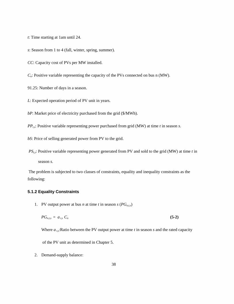
38
t: Time starting at 1am until 24.
s: Season from 1 to 4 (fall, winter, spring, summer).
CC: Capacity cost of PVs per MW installed.
Cn: Positive variable representing the capacity of the PVs connected on bus n (MW).
91.25: Number of days in a season.
L: Expected operation period of PV unit in years.
bP: Market price of electricity purchased from the grid ($/MWh).
PPt,s: Positive variable representing power purchased from grid (MW) at time t in season s.
bS: Price of selling generated power from PV to the grid.
PSt,s: Positive variable representing power generated from PV and sold to the grid (MW) at time t in
season s.
The problem is subjected to two classes of constraints, equality and inequality constraints as the
following:
5.1.2 Equality Constraints
1. PV output power at bus n at time t in season s (PGn,t,s)
PGn,t,s = a t,s Cn (5-2)
Where a t,s:Ratio between the PV output power at time t in season s and the rated capacity
of the PV unit as determined in Chapter 5.
2. Demand-supply balance:
39
k
n
k
n
stnststst PGPSPPDemand1 1
,,,,,
(5-3)
Where
Demand t,s : is the power consumed by the load at time t in season s.
5.1.3 Inequality Constraints
1. Electricity can be either purchased from the grid or sold to the grid:
XSt,s + XBt,s ≤ 1 (5-4)
Where:
otherwise
sseasonintatgridtopowersellingissystemtheifiablebinaryaisXS st
:0
.:1:var,
otherwise
sintatgridthefrompowergpurchaissystemtheifiablebinaryaisXB st
:0
.sin:1:var,
2. Electricity purchase condition at time t in season s is that the system can only purchase
electricity from the grid if the binary variable is 1:
PPt,s ≤ TC XBt,s (5-5)
Where:
TC: The main transformer capacity that is supplying power from the main substation.
3. Electricity sold from PV units condition at time t in season s is that the micro-grid can only
sell electricity to the utility if the binary variable is 1:
PSt,s ≤ TC XSt,s (5-6)
40
4. Capacity limit of PV unit to be connected to bus n:
Cn≤1MW (5-7)
5. Total capacity of PV units:
MWCn
n 10
(5-8)
5.2 13 bus Feeder Case Study
PV units are to be allocated and sized for 13 bus distribution system provided in Figure 5-1. The
system presented here is a modified version of the IEEE 13 bus feeder. The regulator in the original
system connecting buses 1 and 4 is neglected. Moreover, in the original system an intermediate node
between node 9 and 10 is present. This node is connected to node 9 through a switch that has been
removed in the system under study. Bus 13 has been added as the substation transformer is to connect
bus 1 and bus 13. Capacitors are connected to buses 10 and 7 in the original system, but their
presence here has been neglected. Furthermore, all the lines in the system are assumed to be three
phase lines which is not the case in the original system. It is important to emphasize that any
conductance available in the original system has been neglected and the resistance and the inductance
of any line of the system have been assumed to follow the line data presented in Chapter 6. The main
substation is located at bus 13 with a capacity of 5000KVA in the demand-supply balance without
power flow feeder representation case study; while it has a value higher than that under AC power
balance with the representation of feeder power flow. Spot loads are located at buses 6, 3, 2, 11, 9, 10
and 7 [72]. The distributed load is neglected. These modifications have been considered for
simplicity reasons. Moreover, due to the nature of the problem being solved under the AC power
balance with feeder power flow representation modeled as mixed integer non linear programming
problem that is non convex, and since the accessible solvers for MINLP in the selected simulation
tool, GAMS, can solve non convex problems with limited capacity, the problem is solved with SBB
solver with the capability of solving convex problems. This might result in a local optimal solution
that can be avoided with certain modification in the system such that the optimization problem
formulation would provide a solution and infeasibility is avoided.

41
2 3 4 5 6
1
107 8
11
9
12
13
Figure 5-1 13 bus radial feeder after modifications to IEEE 13 bus feeder for simplicity reasons
5.2.1 Substation Transformer
Considering the grid to supply the local distribution company represented by the system below bus 1
through a transformer, the capacity of this transformer is to be determined. In general, the
transformer rating is the substation capacity that is 5000KVA. This would mean as well that the
substation can supply a maximum of 5000KW load [73]
5.2.2 Load
The actual demands of IEEE 13 bus system are provided in Table 5-1. Only spot loads of the system
are calculated; while distributed loads are neglected in the analysis.
Table 5-1Peak demands
Bus
Spot load
(MW)
Spot load
(MVAR)
6 0.4 0.29
3 0.17 0.125
2 0.23 0.132
11 0.128 0.086
9 1.325 0.811
10 0.843 0.462
7 0.17 0.08
Total 3.266 1.986
42
A typical 24 hours load profile in different seasons (fall, winter, spring, summer) is provided in Table
5-2. The data has been assumed to follow a similar system and they are taken from [74] that has been
and published in [75]. The data is expressed as a fraction of the peak load. It can be noted from this
table that the maximum power demand takes place between 5pm and 7pm in winter, 1pm and 3pm in
spring, and 7pm and 8pm in summer and Table 5-3 presents the load data of the system shown in
Figure 5-1during the four terms of the year winter, spring, summer and fall. These are expressed as a
fraction of the total peak load of the system. It can be noted from this table that the maximum power
demand by the load occurs between (9am-10am) and (11am-12pm) in fall, (4pm-5pm) in winter,
(9am-10am) and (11am-12pm) in spring and (11am-12pm) and (1pm-3pm) in summer.
The actual demand of the IEEE 13 bus system for 24 hours in different seasons of the year is to be
calculated using the following equation:
Demand (i,t,s) = DP(i) X %L(t,s) ( 5-9)
Where
Demand(i,t,s): Actual demand of the system at bus i, time t and season s.
t : Time (certain hour, 12am-12pm & 12pm-12am) at which load is consumed.
s: Season of the year (fall, winter, spring, summer).
DP(i): Peak demand at bus i obtained from the distribution system spot load data.
%L(t,s): typical load profile of Ontario at time t and season s as a percentage of the peak demand.

43
Table 5-2 Typical 24 hours load profile in four seasons (%).
Taken from[74], [75]
Hour Fall Winter Spring Summer
12-1 am 0.3717 0.4757 0.3969 0.64
1—2 0.3658 0.4473 0.3906 0.6
2—3 0.354 0.426 0.378 0.58
3—4 0.3422 0.4189 0.3654 0.56
4—5 0.3481 0.4189 0.3717 0.56
5—6 0.3835 0.426 0.4095 0.58
6—7 0.4248 0.5254 0.4536 0.64
7—8 0.5015 0.6106 0.5355 0.76
8—9 0.5605 0.6745 0.5985 0.87
9—10 0.5841 0.6816 0.6237 0.95
10—11 0.59 0.6816 0.63 0.99
11-12pm 0.5841 0.6745 0.6237 1
12—1 0.5487 0.6745 0.5859 0.99
1—2 0.5428 0.6745 0.5796 1
2—3 0.531 0.6603 0.567 1
3—4 0.5192 0.6674 0.5544 0.97
4—5 0.531 0.7029 0.567 0.96
5—6 0.5428 0.71 0.5796 0.96
6—7 0.5664 0.71 0.6048 0.93
7—8 0.5782 0.6816 0.6174 0.92
8—9 0.5664 0.6461 0.6048 0.92
9—10 0.531 0.5893 0.567 0.93
10—11 0.472 0.5183 0.504 0.87
11-12am 0.413 0.4473 0.441 0.72
5.3 Results based on Demand-Supply Balance without Feeder Power Flow
Representation for13 Bus Radial Feeder
The results for three types of study are presented in this section. In the first subsection, the price at
which the PV units would sell electricity to the grid is considered to be fixed and an investigation on
the corresponding PV operation period at which the 13 bus radial feeder would allocate PV units in
the system or sell electricity to the grid is carried out. In the second subsection, the price at which the

44
electricity would be sold from PV units to grid after meeting system demands is allowed to vary at
fixed operation period of PV. The capital cost at both studies is set to be invariable. In the third
subsection, the capital cost variation effect on the age at which the system would allocate PV units or
sell electricity to the grid is considered.
5.3.1 Objective Function With Respect to PV Operation Period
The objective function is to be minimized in this work. This objective function is a function of the
operation period of the PV units. The operation period of the PV units has been set to vary between 1
year and 30 years. The objective function corresponding to such variation was determined through the
optimization problem. The results have been displayed in Figure 5-2.
Figure 5-2 Electricity cost with respect to PV operation period.
It can be noted that for the set data used in the problem, the total cost of electricity purchased from
the grid is a positive number and keeps increasing until a maximum point where the cost switches to
decrease. When the operation period of PV units is considered to be 28years, it can be noted that the
cost becomes negative. This can be explained as the following:
When the operation period of PV was set to be between 1 and 19 years, no PV units were
allocated in the13bus feeder. This is because the installation cost of PV/MW is very high
and the operation of PV over these years would not result in any revenue. In other words, it
is preferable to purchase electricity from the grid rather than supplying it from PV units

45
since the optimization problem is a minimization problem targeting minimizing the total
cost of electricity purchased from the grid and involving the initial cost of PV. If the PV
units are to be operating in such system, 18 years would not be sufficient to pay for the
capital cost of PV. That is the main reason for having a positive cost that is increasing over
the years.
When the operation period of PV was set to be 20 years, PV units were allocated and sized in
the 13bus feeder, as the capacity of the PV unit is s function of the bus at which it is
installed as shown in the objective function presented in equation (5-1). The location of the
PV units is considered in the optimization problem formulation as the capacity of the PV
unit at certain bus is involved in equation (5-2) and this equation is involved in the demand-
supply balance equation (5-3). The cost of electricity purchased from the grid per year
decreased in comparison to the cost at 19 years. This is because the PV units have been
allocated and sized to minimize the total cost of electricity. With the allocation and sizing of
PV units in the feeder, the load started to be supplied by the PV units and less MWh were to
be purchased from the grid. This leads to a reduction in the cost compared to the previous
case.
For an operation period of 28 years, the PV units system is capable of paying back the
capital cost of the PV which has been reflected back into the total cost such that the
objective function become negative. However, the payback time seems to be high when
compared to what is claimed in practice. This is due to two main factors:
A) The PV capacity factor varies between 0 and a maximum value of 0.665689 in
summer season. It is important to note that this factor would differ based on weather
conditions and the area in which the study is performed.
B) The optimization model is set such that the system could supply its demands from
the power generated from PV units at first and then sell electricity to the grid in case of
extra generation.
5.3.2 Allocation and Sizing of PV Units
Running the optimization problem using GAMS software for different PV operation periods, the
optimal location and size of PV units are determined as shown in Table 5-3 and Table 5-4.
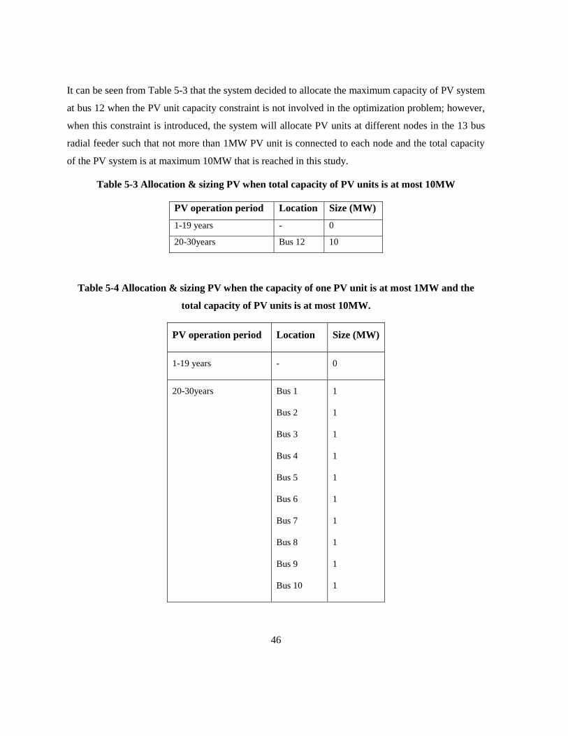
46
It can be seen from Table 5-3 that the system decided to allocate the maximum capacity of PV system
at bus 12 when the PV unit capacity constraint is not involved in the optimization problem; however,
when this constraint is introduced, the system will allocate PV units at different nodes in the 13 bus
radial feeder such that not more than 1MW PV unit is connected to each node and the total capacity
of the PV system is at maximum 10MW that is reached in this study.
Table 5-3 Allocation & sizing PV when total capacity of PV units is at most 10MW
PV operation period Location Size (MW)
1-19 years - 0
20-30years Bus 12 10
Table 5-4 Allocation & sizing PV when the capacity of one PV unit is at most 1MW and the
total capacity of PV units is at most 10MW.
PV operation period Location Size (MW)
1-19 years - 0
20-30years Bus 1
Bus 2
Bus 3
Bus 4
Bus 5
Bus 6
Bus 7
Bus 8
Bus 9
Bus 10
1
1
1
1
1
1
1
1
1
1
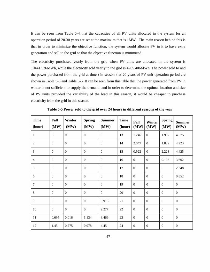
47
It can be seen from Table 5-4 that the capacities of all PV units allocated in the system for an
operation period of 20-30 years are set at the maximum that is 1MW. The main reason behind this is
that in order to minimize the objective function, the system would allocate PV in it to have extra
generation and sell to the grid so that the objective function is minimized.
The electricity purchased yearly from the grid when PV units are allocated in the system is
10441.526MWh, while the electricity sold yearly to the grid is 4265.406MWh. The power sold to and
the power purchased from the grid at time t in season s at 20 years of PV unit operation period are
shown in Table 5-5 and Table 5-6. It can be seen from this table that the power generated from PV in
winter is not sufficient to supply the demand, and in order to determine the optimal location and size
of PV units provided the variability of the load in this season, it would be cheaper to purchase
electricity from the grid in this season.
Table 5-5 Power sold to the grid over 24 hours in different seasons of the year
Time Fall Winter Spring Summer Time Fall Winter
Spring Summer
(hour) (MW) (MW) (MW) (MW) (hour) (MW) (MW) (MW) (MW)
1 0 0 0 0 13 1.246 0 1.987 4.575
2 0 0 0 0 14 2.047 0 1.829 4.923
3 0 0 0 0 15 0.922 0 2.228 4.425
4 0 0 0 0 16 0 0 0.103 3.602
5 0 0 0 0 17 0 0 0 2.348
6 0 0 0 0 18 0 0 0 0.852
7 0 0 0 0 19 0 0 0 0
8 0 0 0 0 20 0 0 0 0
9 0 0 0 0.915 21 0 0 0 0
10 0 0 0 2.277 22 0 0 0 0
11 0.695 0.016 1.134 3.466 23 0 0 0 0
12 1.45 0.275 0.978 4.45 24 0 0 0 0

48
Table 5-6 Power purchased from the grid at time t in season s in typical days of the year
Time
(hour)
Fall
(MW)
Winter
(MW)
Spring
(MW)
Summer
(MW)
Time
(hour)
Fall
(MW)
Winter
(MW)
Spring
(MW)
Summer
(MW)
1 1.461 1.276 1.96 1.195 13 0 0.15 0 0
2 1.391 1.235 1.894 1.156 14 0 0.033 0 0
3 1.368 1.193 1.829 1.118 15 0 0.626 0 0
4 1.368 1.214 1.829 1.137 16 0.016 1.278 0 0
5 1.391 1.337 1.894 1.253 17 1.27 1.659 0.615 0
6 1.716 1.481 2.09 1.387 18 2.13 1.938 1.83 0
7 1.994 1.749 2.407 1.366 19 2.226 2.016 2.816 0.651
8 2.135 1.955 2.306 0.472 20 2.11 1.975 3.005 1.661
9 1.411 1.871 2.355 0 21 1.925 1.852 3.037 1.734
10 0.362 1.008 0.833 0 22 1.693 1.646 2.841 1.542
11 0 0 0 0 23 1.461 1.44 2.352 1.349
12 0 0 0 0 24 1.554 1.296 2.09 1.214
5.3.3 Capital Cost Reduction over Years under Demand-Supply Balance without
Feeder Power Flow Representation
Since the capital cost of PV units is expected to reduce over year, the question arises: what would
happen if the set price at which the utility is purchasing electricity from the system is set to be fixed at
$420/MWh. Table 5-7 presents the simulation results obtained by reducing the PV capital cost. It can
be seen that as the PV capital cost decreases, the operation period at which PV units are allocated in
the system to supply its demand and then to sell extra generation to the grid decreases. The model
presented could be a good tool, for utilities, to modify the PV selling price as PV capital cost
decreases.
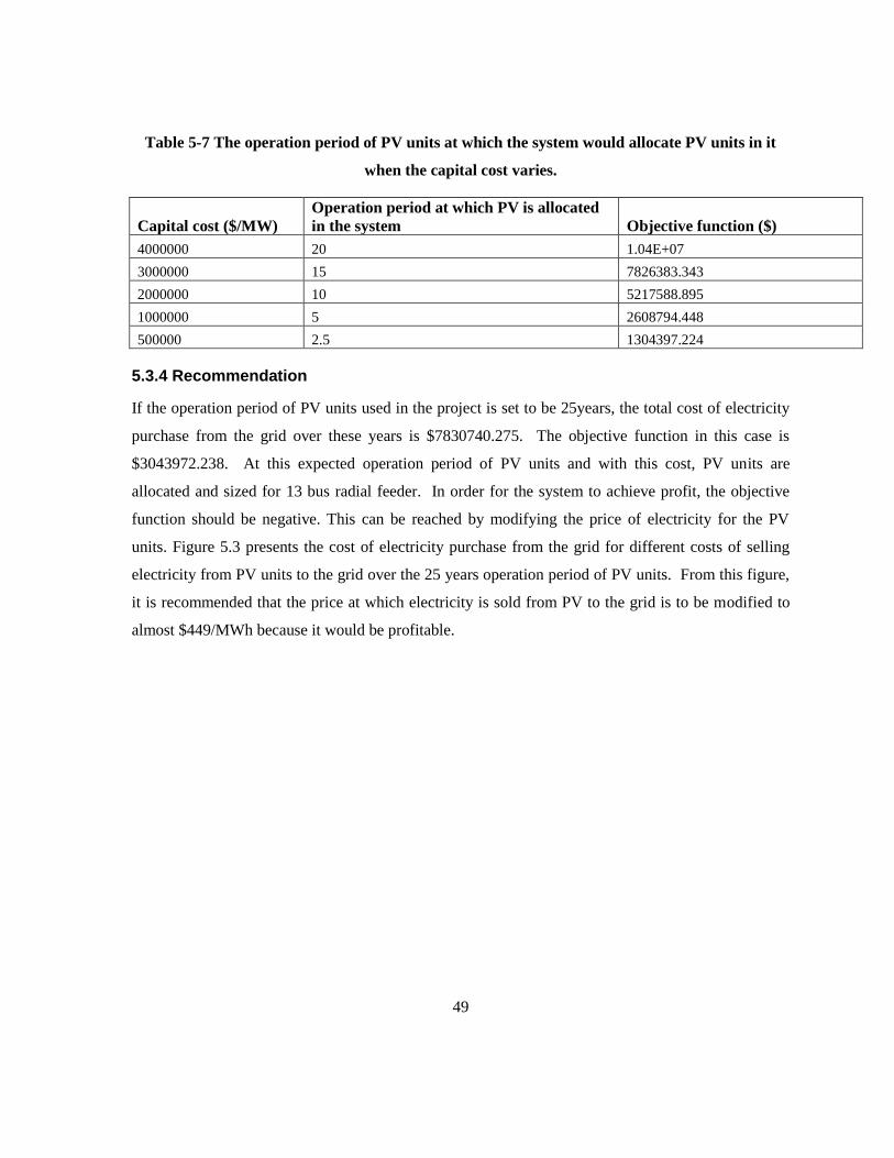
49
Table 5-7 The operation period of PV units at which the system would allocate PV units in it
when the capital cost varies.
Capital cost ($/MW)
Operation period at which PV is allocated
in the system Objective function ($)
4000000 20 1.04E+07
3000000 15 7826383.343
2000000 10 5217588.895
1000000 5 2608794.448
500000 2.5 1304397.224
5.3.4 Recommendation
If the operation period of PV units used in the project is set to be 25years, the total cost of electricity
purchase from the grid over these years is $7830740.275. The objective function in this case is
$3043972.238. At this expected operation period of PV units and with this cost, PV units are
allocated and sized for 13 bus radial feeder. In order for the system to achieve profit, the objective
function should be negative. This can be reached by modifying the price of electricity for the PV
units. Figure 5.3 presents the cost of electricity purchase from the grid for different costs of selling
electricity from PV units to the grid over the 25 years operation period of PV units. From this figure,
it is recommended that the price at which electricity is sold from PV to the grid is to be modified to
almost $449/MWh because it would be profitable.

50
Figure 5-3 Study on variation on the price of electricity sold from PV to the grid.
In this work, two terms are defined. The first term is the location price and the second term is the
selling price. The location price is the set PV electricity selling price at which the system will decide
to allocate PV units based on the optimization problem without achieving any profit. The selling price
is the price at which the objective function will become negative and the system will achieve profit.
At this price, the PV units already exist in the system. These terms and the corresponding objective
functions are determined for different PV units’ operation period as shown in Table 5-8 considering
the capital cost to be fixed and it is to be recovered over these years.
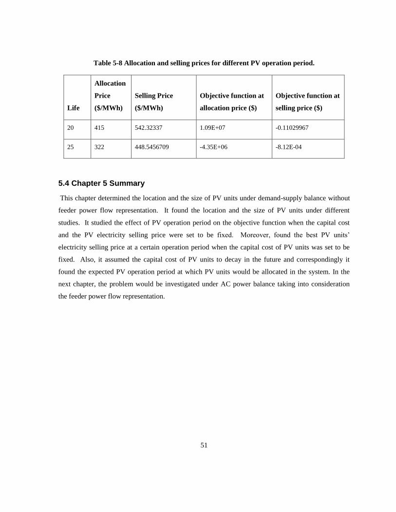
51
Table 5-8 Allocation and selling prices for different PV operation period.
Life
Allocation
Price
($/MWh)
Selling Price
($/MWh)
Objective function at
allocation price ($)
Objective function at
selling price ($)
20 415 542.32337 1.09E+07 -0.11029967
25 322 448.5456709 -4.35E+06 -8.12E-04
5.4 Chapter 5 Summary
This chapter determined the location and the size of PV units under demand-supply balance without
feeder power flow representation. It found the location and the size of PV units under different
studies. It studied the effect of PV operation period on the objective function when the capital cost
and the PV electricity selling price were set to be fixed. Moreover, found the best PV units’
electricity selling price at a certain operation period when the capital cost of PV units was set to be
fixed. Also, it assumed the capital cost of PV units to decay in the future and correspondingly it
found the expected PV operation period at which PV units would be allocated in the system. In the
next chapter, the problem would be investigated under AC power balance taking into consideration
the feeder power flow representation.

52
Chapter 6
Optimal Sizing & Location of PV Units under AC Power Balance
with Feeder Power Flow Representation
Real power systems are operated under AC power balance. The main objective of this section is to
optimally allocate and size PV units while considering the optimal AC power balance. The objective
of the optimal power balance is to minimize the total cost of electricity generation by optimally
allocating and sizing PV units to increase the power generated from them in order to satisfy the
demand and selling extra generation to the grid. In this section, the problem formulation is provided
and the results are analyzed investigating the effect of PV operation period on the objective.
Furthermore, it looks for the best PV electricity selling price under which the PV will be allocated in
the 13 bus radial feeder system. Since the capital cost of PV units is expected to drop over the years
and assuming that the utility is fixing the price at which it purchases electricity generated from PV
units, the PV operation period at which the system will decide to allocate them in it and the PV
operation period at which the system will be able to achieve profit are determined.
6.1 Problem Formulation
The objective function and constraints for the optimal allocation and sizing of PV units for 13 radial
feeder that is provided in the following subsections:
6.1.1 Objective Function
The objective function is to minimize the total cost of electricity generation as shown below:
M
i s t s t
ststst PsexbsbasexDxlifPPbPebasexDxlifiCCCt1
4
1
24
1
4
1
24
1
,,,)(cosmin
(6-1)
Where
Cost : total cost of electricity generation from the substation located at bus 13 in case of 13 bus
feeder.
CC: capital cost of PV per MW approximated to be 4X10⁶ as in section 4.6.
i: bus number (integer: i=1,…..,13.) for 13 bus system.

53
M: bus number 1 in case of 13 bus feeder.
C(i): capacity of PV Unit in MW allocated at bus i.
base: since the power balance is run to be in per unit system, the power is multiplied back by the base
unit that is 5000KVA such that the output of multiplication is in MW.
D: number of days in a season considering the year to be made of 365 days.
life: PV unit operation period.
s: seasons of the year (fall, winter, spring and summer).
t: hours of the day that is an integer number (t=1,….24).
bPt,s:price of electricity purchased from the market at time t in season s. This price is considered to be
fixed in the demand-supply balance case study; while it is set to be fixed to in the AC power balance
case study for simplicity.
PPt,s: power purchased from the grid at time t in season s to meet the hourly demands of the system in
measured in per unit and it is a free variable.
bs: price of electricity generated from PV units and sold back to the grid.
Pst,s: power sold from PV units to the grid at time t in season s measured in per unit and it is a free
variable.
6.1.2 Constraints
The optimization problem is subject to two classes of constraints that are the equality constraints and
the inequality constraints.
1. Equality constraints
These constraints include the parameters of power balance constraints, system losses, power
transmitted from substation to bus 1 in the 13 bus system, energy purchased from grid and energy
sold from PV units to the grid.
Power balance Parameters constraints:
0,, stMi (6-2)
04.1,, stMiV (6-3)

54
The upper and lower levels on the voltage at different busses at different times in different seasons are
inequality constraints but they are set as equality constraints as programmed in GAMS software as in
the following:
05.1)(,, upperV sti (6-4)
8.0)(,, lowerV sti (6-5)
The main reason behind setting the lower limit on the voltage to 0.8, that is a low voltage value not
preferable in practice, is to relax the constraint to avoid infeasibility. This would lead certain nodes in
the 13 bus feeder to experience a low voltage at certain instances of time. The location of PV units
might be at these nodes that might be considered a problem. A reason behind the voltage drop at
certain nodes, to which a PV unit is connected with the setting of the lower limit on the voltage to be
0.8, is that the IEEE standards do not allow PV system to generate reactive power that can be a
solution to the problem faced under this case. Other factors for experiencing low voltage at certain
nodes in the system with the set lower limit on the voltage are the load factor and the capacity factor
of the PV units. Moreover, the nodes experiencing low voltages at certain instances of time are the
end of the line nodes. This problem can be solved by integrating capacitors or voltage regulators to
the nodes with low voltage.
Total system losses constraint:
losses=
M
j
stistjstjstistjstiji
M
its
VVVVG1
,,,,,,,,,,2
,,2
),(
1
24
1
4
1
))(cos2(5.0
(6-6) [74]
Active AC load flow constraint (modified from the original load flow equation [76] to
include the load flow at time t in season s and to include the power generated from PV unit):
M
j
stistjjijistjstististsti YVVdemandbaseiCaP1
,,,,),(),(,,,,,,,,, )(cos)/)((
(6-7)
The voltages at different nodes play a role in determining the location of the PV unit in the system as
the capacity of the PV unit at a certain node is a part of the active AC load flow constraint. Moreover,
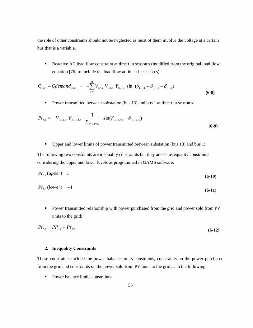
55
the role of other constraints should not be neglected as most of them involve the voltage at a certain
bus that is a variable.
Reactive AC load flow constraint at time t in season s (modified from the original load flow
equation [76] to include the load flow at time t in season s):
M
j
stistjjijistjstististi YVVQdemandQ1
,,,,),(),(,,,,,,,, )(sin
(6-8)
Power transmitted between substation (bus 13) and bus 1 at time t in season s:
)sin(1
,,1,,13
13,1
,,13,,1, stjsti
ji
stjstistX
VVPt
(6-9)
Upper and lower limits of power transmitted between substation (bus 13) and bus 1:
The following two constraints are inequality constraints but they are set as equality constraints
considering the upper and lower levels as programmed in GAMS software:
1)(, upperPt st (6-10)
1)(, lowerPt st (6-11)
Power transmitted relationship with power purchased from the grid and power sold from PV
units to the grid:
ststst PsPPPt ,,, (6-12)
2. Inequality Constraints
These constraints include the power balance limits constraints, constraints on the power purchased
from the grid and constraints on the power sold from PV units to the grid as in the following:
Power balance limits constraints:
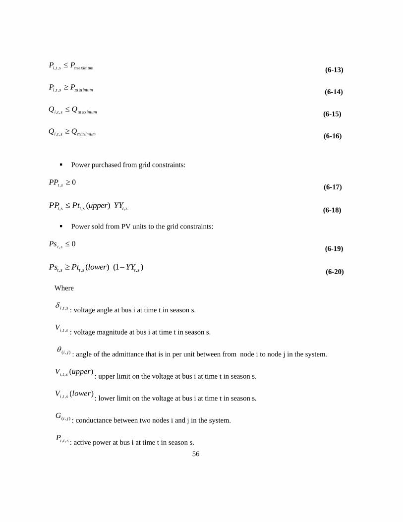
56
imumsti PP max,, (6-13)
imumsti PP min,, (6-14)
imumsti QQ max,, (6-15)
imumsti QQ min,, (6-16)
Power purchased from grid constraints:
0, stPP (6-17)
ststst YYupperPtPP ,,, )( (6-18)
Power sold from PV units to the grid constraints:
0, stPs (6-19)
)1()( ,,, ststst YYlowerPtPs (6-20)
Where
sti ,,: voltage angle at bus i at time t in season s.
stiV ,, : voltage magnitude at bus i at time t in season s.
),( ji: angle of the admittance that is in per unit between from node i to node j in the system.
)(,, upperV sti : upper limit on the voltage at bus i at time t in season s.
)(,, lowerV sti : lower limit on the voltage at bus i at time t in season s.
),( jiG: conductance between two nodes i and j in the system.
stiP ,, : active power at bus i at time t in season s.
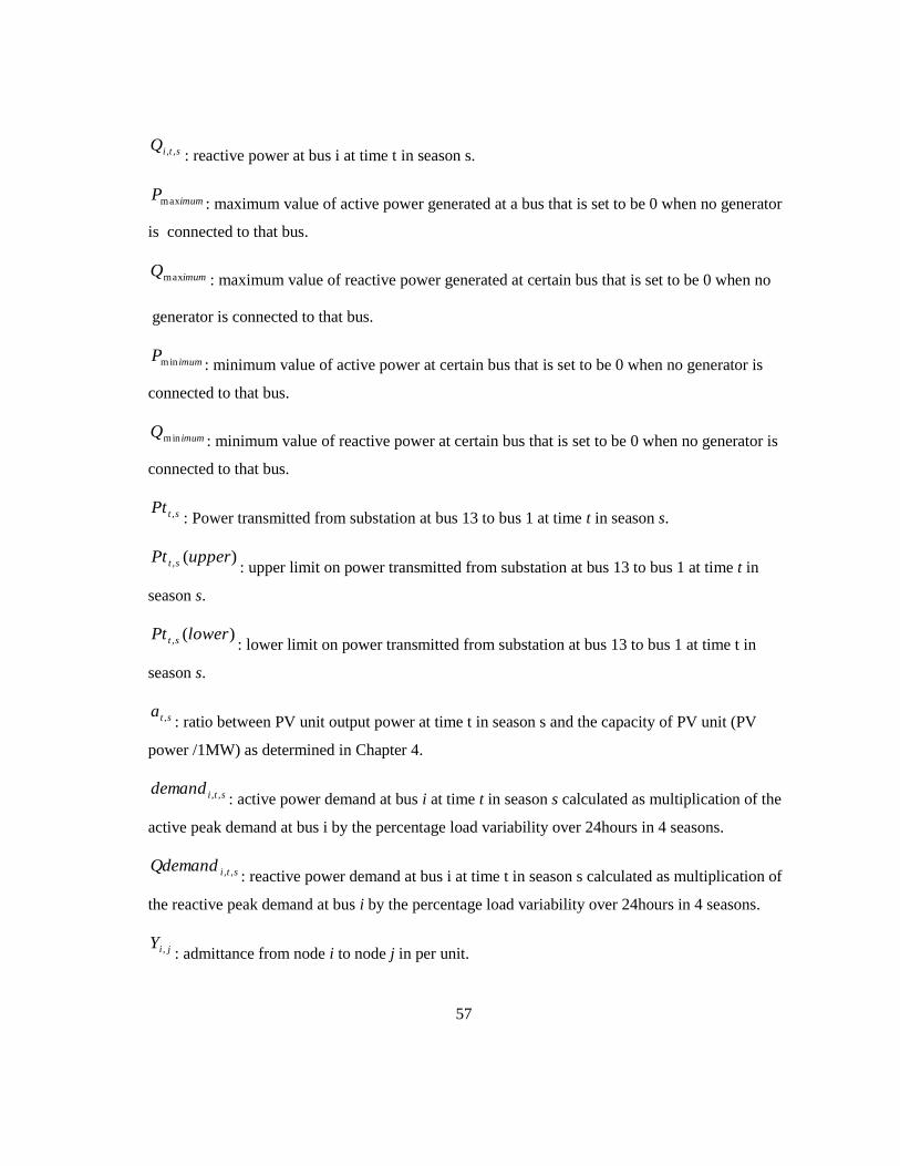
57
stiQ ,, : reactive power at bus i at time t in season s.
imumPmax : maximum value of active power generated at a bus that is set to be 0 when no generator
is connected to that bus.
imumQmax : maximum value of reactive power generated at certain bus that is set to be 0 when no
generator is connected to that bus.
imumPmin : minimum value of active power at certain bus that is set to be 0 when no generator is
connected to that bus.
imumQmin : minimum value of reactive power at certain bus that is set to be 0 when no generator is
connected to that bus.
stPt , : Power transmitted from substation at bus 13 to bus 1 at time t in season s.
)(, upperPt st : upper limit on power transmitted from substation at bus 13 to bus 1 at time t in
season s.
)(, lowerPt st : lower limit on power transmitted from substation at bus 13 to bus 1 at time t in
season s.
sta , : ratio between PV unit output power at time t in season s and the capacity of PV unit (PV
power /1MW) as determined in Chapter 4.
stidemand ,, : active power demand at bus i at time t in season s calculated as multiplication of the
active peak demand at bus i by the percentage load variability over 24hours in 4 seasons.
stiQdemand ,, : reactive power demand at bus i at time t in season s calculated as multiplication of
the reactive peak demand at bus i by the percentage load variability over 24hours in 4 seasons.
jiY , : admittance from node i to node j in per unit.

58
stYY , : binary variable (0 or 1) at time t in season s based on which either the power would be
purchased from the grid or sold from PV units to the grid at time t in season s.
6.2 Systems Parameters
Since AC power balance is considered, the system line data and loads (spot loads) in PU for the 13
radial bus feeder is presented in Table 6-1 and Table 6-2:
Table 6-1 Line data for the 13bus radial feeder.
From To R (PU) X(PU) Charging Length of the line (feet)
1 4 0.0369 0.1147 0 2000
2 3 0.0123 0.0197 0 300
3 4 0.0205 0.0328 0 500
4 5 0.0205 0.0328 0 500
4 9 0.0369 0.1147 0 2000
8 9 0.0130 0.0066 0 300
7 8 0.0130 0.0066 0 300
9 10 0.0216 0.0111 0 500
9 12 0.0185 0.0573 0 1000
8 11 0.0345 0.0177 0 800
1 13 0 0.0800 0 Transformer (0)
6 5 0.0011 0.0020 0 Transformer (0)
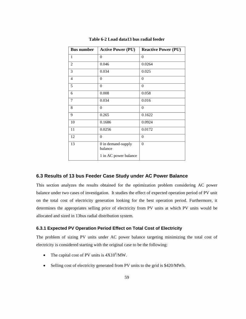
59
Table 6-2 Load data13 bus radial feeder
Bus number Active Power (PU) Reactive Power (PU)
1 0 0
2 0.046 0.0264
3 0.034 0.025
4 0 0
5 0 0
6 0.008 0.058
7 0.034 0.016
8 0 0
9 0.265 0.1622
10 0.1686 0.0924
11 0.0256 0.0172
12 0 0
13 0 in demand-supply
balance
1 in AC power balance
0
6.3 Results of 13 bus Feeder Case Study under AC Power Balance
This section analyzes the results obtained for the optimization problem considering AC power
balance under two cases of investigation. It studies the effect of expected operation period of PV unit
on the total cost of electricity generation looking for the best operation period. Furthermore, it
determines the appropriates selling price of electricity from PV units at which PV units would be
allocated and sized in 13bus radial distribution system.
6.3.1 Expected PV Operation Period Effect on Total Cost of Electricity
The problem of sizing PV units under AC power balance targeting minimizing the total cost of
electricity is considered starting with the original case to be the following:
The capital cost of PV units is 4X10⁶/MW.
Selling cost of electricity generated from PV units to the grid is $420/MWh.

60
PV units’ operation period is set to 10 years.
Targeting the objective, the results for this case were as the following:
There were no PV units allocated in the system under the set operation period.
The total cost of electricity was $5.52X10⁶ for the 10 years of operation.
The energy transmitted from the grid to the system is the energy purchased from the grid and
it is 1.812285X10⁴MWh yearly; while this case does not include any selling to the grid as
there was no PV in the system.
If the operation period of PV is modified while fixing the capital cost and the set PV electricity
selling price, the objective function would be increasing linearly until PV units are allocated in the
system and that would take place around 33 years of PV operation period which does not take place
in practice as PV operation period is expected to reach 25 years [77] as shown in Figure 6-1. This is
represented by the point after which the curve starts decaying. This is due to the fact that the system
will not be able to recover its capital cost over the expected PV operation period with the set PV
electricity selling price considering AC power losses. The power purchased at time t in season s at 10
years of PV operation period is shown in Table 6-3.
Figure 6-1: Objective function with respect to PV operation period

61
Table 6-3 Power purchased in per unit (PU) from grid when PV operation period is 10
Time
Hour
Fall
(PU)
Winter
(PU)
Spring
(PU)
Summer
(PU)
Time
Hour
Fall
(PU)
Winter
(PU)
Spring
(PU)
Summer
(PU) 1 0.299605 0.260692 0.406087 0.243769 13 0.459054 0.391707 0.701203 0.365892
2 0.28495 0.252087 0.391988 0.235737 14 0.448901 0.38285 0.701203 0.357648
3 0.280075 0.243497 0.377938 0.227717 15 0.453974 0.374012 0.677952 0.349419
4 0.280075 0.24779 0.377938 0.231726 16 0.479444 0.38285 0.670254 0.357648
5 0.28495 0.273628 0.391988 0.255842 17 0.48456 0.391707 0.670254 0.365892
6 0.353741 0.303948 0.434435 0.284126 18 0.48456 0.409478 0.647305 0.382429
7 0.413579 0.36079 0.520803 0.337105 19 0.464141 0.418393 0.639702 0.390722
8 0.459054 0.405028 0.602015 0.378289 20 0.438776 0.409478 0.639702 0.382429
9 0.464141 0.422858 0.66258 0.394875 21 0.398538 0.38285 0.647305 0.357648
10 0.464141 0.427329 0.693426 0.399032 22 0.348792 0.338842 0.602015 0.316656
11 0.459054 0.422858 0.701203 0.394875 23 0.299605 0.295265 0.491778 0.276028
12 0.459054 0.396142 0.693426 0.37002 24 0.319216 0.265001 0.434435 0.24779
The power transmitted at time t in season s at 33years of PV operation period is presented in Table 6-
4. The positive values correspond to the power purchase from the grid to supply the system; while the
negative values represent the power sold to the grid from the system at time t in season s due to extra
generation from PV units.
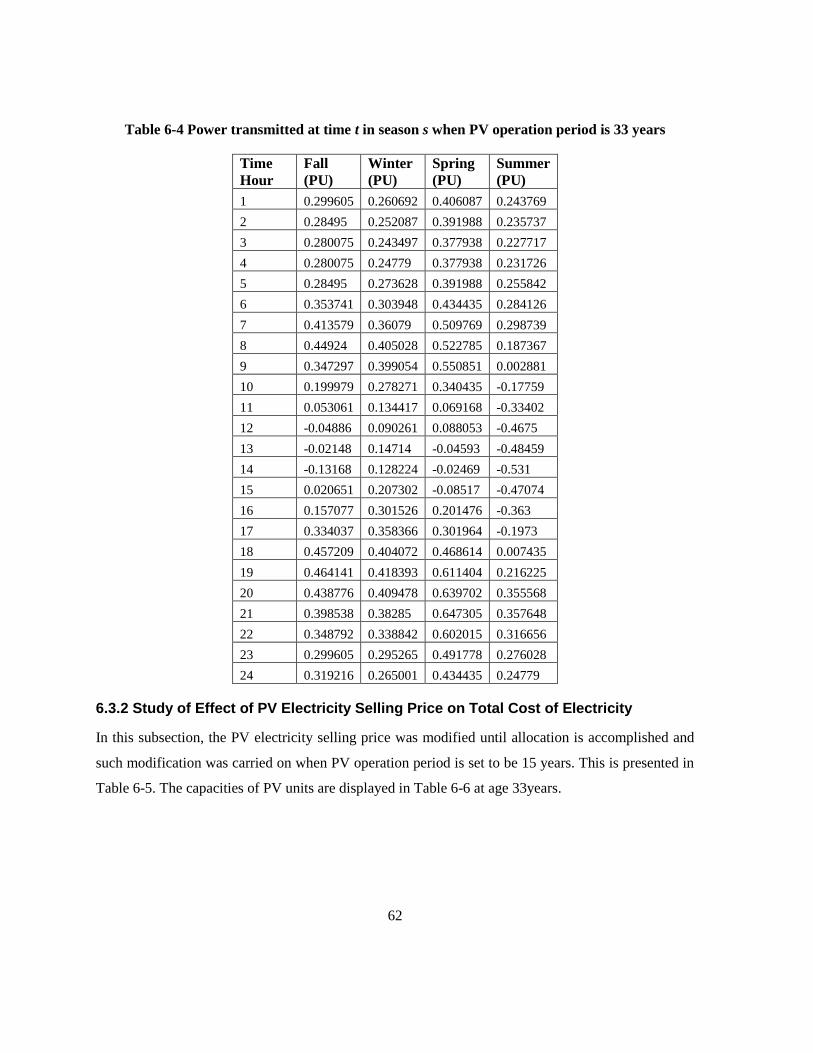
62
Table 6-4 Power transmitted at time t in season s when PV operation period is 33 years
Time
Hour
Fall
(PU)
Winter
(PU)
Spring
(PU)
Summer
(PU)
1 0.299605 0.260692 0.406087 0.243769
2 0.28495 0.252087 0.391988 0.235737
3 0.280075 0.243497 0.377938 0.227717
4 0.280075 0.24779 0.377938 0.231726
5 0.28495 0.273628 0.391988 0.255842
6 0.353741 0.303948 0.434435 0.284126
7 0.413579 0.36079 0.509769 0.298739
8 0.44924 0.405028 0.522785 0.187367
9 0.347297 0.399054 0.550851 0.002881
10 0.199979 0.278271 0.340435 -0.17759
11 0.053061 0.134417 0.069168 -0.33402
12 -0.04886 0.090261 0.088053 -0.4675
13 -0.02148 0.14714 -0.04593 -0.48459
14 -0.13168 0.128224 -0.02469 -0.531
15 0.020651 0.207302 -0.08517 -0.47074
16 0.157077 0.301526 0.201476 -0.363
17 0.334037 0.358366 0.301964 -0.1973
18 0.457209 0.404072 0.468614 0.007435
19 0.464141 0.418393 0.611404 0.216225
20 0.438776 0.409478 0.639702 0.355568
21 0.398538 0.38285 0.647305 0.357648
22 0.348792 0.338842 0.602015 0.316656
23 0.299605 0.295265 0.491778 0.276028
24 0.319216 0.265001 0.434435 0.24779
6.3.2 Study of Effect of PV Electricity Selling Price on Total Cost of Electricity
In this subsection, the PV electricity selling price was modified until allocation is accomplished and
such modification was carried on when PV operation period is set to be 15 years. This is presented in
Table 6-5. The capacities of PV units are displayed in Table 6-6 at age 33years.
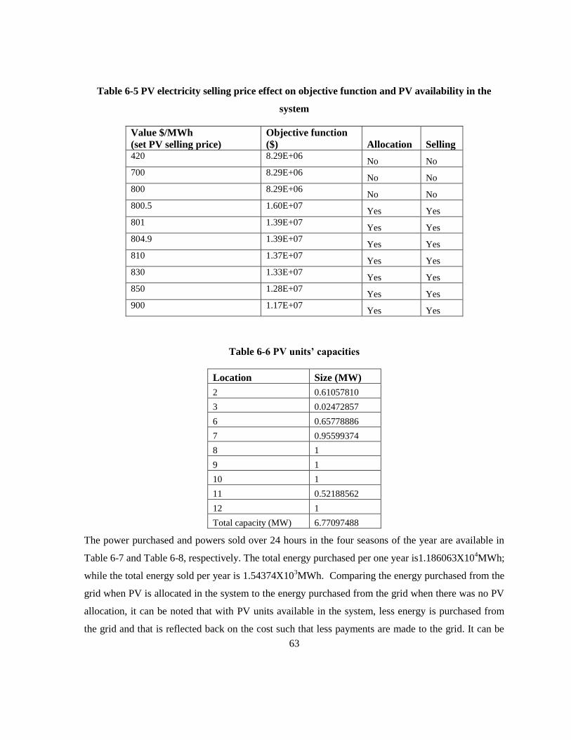
63
Table 6-5 PV electricity selling price effect on objective function and PV availability in the
system
Value $/MWh
(set PV selling price)
Objective function
($) Allocation Selling 420 8.29E+06
No No
700 8.29E+06 No No
800 8.29E+06 No No
800.5 1.60E+07 Yes Yes
801 1.39E+07 Yes Yes
804.9 1.39E+07 Yes Yes
810 1.37E+07 Yes Yes
830 1.33E+07 Yes Yes
850 1.28E+07 Yes Yes
900 1.17E+07 Yes Yes
Table 6-6PVunits’capacities
Location Size (MW)
2 0.61057810
3 0.02472857
6 0.65778886
7 0.95599374
8 1
9 1
10 1
11 0.52188562
12 1
Total capacity (MW) 6.77097488
The power purchased and powers sold over 24 hours in the four seasons of the year are available in
Table 6-7 and Table 6-8, respectively. The total energy purchased per one year is1.186063X104MWh;
while the total energy sold per year is 1.54374X10³MWh. Comparing the energy purchased from the
grid when PV is allocated in the system to the energy purchased from the grid when there was no PV
allocation, it can be noted that with PV units available in the system, less energy is purchased from
the grid and that is reflected back on the cost such that less payments are made to the grid. It can be
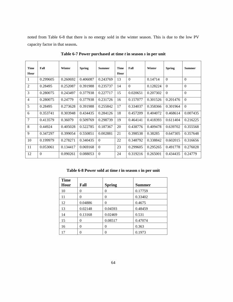
64
noted from Table 6-8 that there is no energy sold in the winter season. This is due to the low PV
capacity factor in that season.
Table 6-7 Power purchased at time t in season s in per unit
Time
Hour
Fall
Winter
Spring
Summer
Time
Hour
Fall
Winter
Spring
Summer
1 0.299605 0.260692 0.406087 0.243769 13 0 0.14714 0 0
2 0.28495 0.252087 0.391988 0.235737 14 0 0.128224 0 0
3 0.280075 0.243497 0.377938 0.227717 15 0.020651 0.207302 0 0
4 0.280075 0.24779 0.377938 0.231726 16 0.157077 0.301526 0.201476 0
5 0.28495 0.273628 0.391988 0.255842 17 0.334037 0.358366 0.301964 0
6 0.353741 0.303948 0.434435 0.284126 18 0.457209 0.404072 0.468614 0.007435
7 0.413579 0.36079 0.509769 0.298739 19 0.464141 0.418393 0.611404 0.216225
8 0.44924 0.405028 0.522785 0.187367 20 0.438776 0.409478 0.639702 0.355568
9 0.347297 0.399054 0.550851 0.002881 21 0.398538 0.38285 0.647305 0.357648
10 0.199979 0.278271 0.340435 0 22 0.348792 0.338842 0.602015 0.316656
11 0.053061 0.134417 0.069168 0 23 0.299605 0.295265 0.491778 0.276028
12 0 0.090261 0.088053 0 24 0.319216 0.265001 0.434435 0.24779
Table 6-8 Power sold at time t in season s in per unit
Time
Hour Fall Spring Summer
10 0 0 0.17759
11 0 0 0.33402
12 0.04886 0 0.4675
13 0.02148 0.04593 0.48459
14 0.13168 0.02469 0.531
15 0 0.08517 0.47074
16 0 0 0.363
17 0 0 0.1973
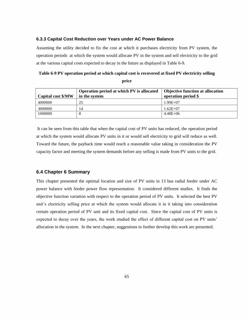
65
6.3.3 Capital Cost Reduction over Years under AC Power Balance
Assuming the utility decided to fix the cost at which it purchases electricity from PV system, the
operation periods at which the system would allocate PV in the system and sell electricity to the grid
at the various capital costs expected to decay in the future as displayed in Table 6-9.
Table 6-9 PV operation period at which capital cost is recovered at fixed PV electricity selling
price
Capital cost $/MW
Operation period at which PV is allocated
in the system
Objective function at allocation
operation period $
4000000 25 1.99E+07
3000000 14 1.62E+07
1000000 8 4.48E+06
It can be seen from this table that when the capital cost of PV units has reduced, the operation period
at which the system would allocate PV units in it or would sell electricity to grid will reduce as well.
Toward the future, the payback time would reach a reasonable value taking in consideration the PV
capacity factor and meeting the system demands before any selling is made from PV units to the grid.
6.4 Chapter 6 Summary
This chapter presented the optimal location and size of PV units in 13 bus radial feeder under AC
power balance with feeder power flow representation. It considered different studies. It finds the
objective function variation with respect to the operation period of PV units. It selected the best PV
unit’s electricity selling price at which the system would allocate it in it taking into consideration
certain operation period of PV unit and its fixed capital cost. Since the capital cost of PV units is
expected to decay over the years, the work studied the effect of different capital cost on PV units’
allocation in the system. In the next chapter, suggestions to further develop this work are presented.

66
Chapter 7
Conclusion & Future Work
In conclusion, the problem of optimal PV sizing and allocation in 13bus system has been considered.
The problem was carried out under both demand-supply balance and AC power balance. The
proposed work sets the basic optimization model suggested to be used for any distribution system
taking into consideration the PV capacity factor and the capability of the system in supplying its loads
first and then selling extra generated power to the grid. The optimization problem is formulated to
minimize the total cost of electricity in the system involving the capital cost of PV units. The work
differs from other previous works in that it determines the payback time of the PV units considering a
more realistic case that involves the variation in the daily solar radiation reflected back into the
system as a PV capacity factor rather than considering the full rating of the PV units. Moreover, the
payback time is different from previous studies as it considers the supplement of the system demands
from the units as a major objective before selling to the grid.
It has been found out that at fixed capital cost of PV units and at fixed PV electricity selling price to
the grid (set by the utility), the total cost of electricity of the system that involves the capital cost of
PV units would keep increasing over years until it reaches a certain age at which the cost would flip
and starts decreasing. This would represent the point after which the system would find it optimal to
allocate PV units such that the total cost of electricity of the system is reduced. Then the study goes
for fixing the operation period of PV units and their capital costs, and determines the prices at which
the system would be able to allocate PV units in the system and the prices at which it would achieve
profit.. In addition, the operation period of PV units at which payback time is found to decrease as the
capital cost of PV units is decreasing (if the utility decides to fix the price at which it purchases PV
electricity from the system), is determined. Since the world is moving toward renewable clean
energy, the utility would gain the advantage of meeting safe environment standards, and the customer
would be willing to achieve profit.
This work can be further extended by taking into consideration the discount rate of the market price.
It can also be applied on the original IEEE 13 bus radial feeder without any modifications such that
all the capacitors and the regulator are involved without the assumption of all the lines to be three

67
phase lines considering a different optimization simulation tool that can be used to solve non convex
problems.
In the future, the approach can be applied on larger distribution systems. It can involve more classes
of renewable energy sources such as wind or combinations of both PV and wind technologies.
68
Bibliography
[1] A. Chambers, ―Distributed generation: a nontechnical guide," PennWell, Tulsa, OK, USA, 2001.
[2] IEA, ―Distributed generation in liberalized electricity markets,‖ Paris, 2002 Page: 128.
[3] T. Ackerman, G. Andersson, L. Soder, ―Distributed generation: a definition,‖. Electric Power
Systems Research, Volume 57, Number 3, 20 April 2001 Page(s). 195-204.
[4] CIRED, ―Dispersed generation, preliminary report of CIRED working group No 4‖, Nice, June
1999.
[5] N. Jenkins, R. Allan, P. Crossley, D. Kirschen and G. Strbac, ’Embedded Generation’,
The Institution of Electrical Engineers, London, United Kingdom, 2000.
[6] European Commission Research,‖Key advantages of distributed energy resources,‖.Available
online at: http://ec.europa.eu/research/energy/nn/nn_rt/nn_rt_dg/article_1159_en.htm
[7]Union Gas, a spectra energy company, ―Distributed generation,‖. Available at:
http://www.uniongas.com/business/gastechnology/productsservices/distributedgen/index.asp
[8]H. Willis, W. Scott,‖Distributed power generation, planning and evaluation,‖ Marcel Dekker Inc,
2000.
[9] History of electricity. Page 42. Available at:
http://www.need.org/needpdf/infobook_activities/IntInfo/Elec3I.pdf
[10] U.S. Department of Energy, ―The potential benefits of distributed generation and the rate-related
issues that may impede its expansion. A study pursuant to section 1817 of the Energy Policy
Act of 2005,‖ 2007 Page(s) 1-188.
[11]L. Lamarre,‖The vision of Distributed Generation,‖.EPRI Journal, Vol 3, 1993 Page(s)7-17.
[12] G. Pepermans, J. Driesen, D Haeseldnockx, W. Dhaseseleer, R. Belmans, ―Distribution
generation: definition, benefits and issues,‖ Energy Policy, Vol 33, 2005 Pages 787-798.
[13] P. Vaessan, D. Thielens, ―Distributed generation: policy and incentives on distributed generation.
69
Leonardo Energy, Kema Consulting, May 2007. Available at:
http://www.leonardo-energy.org/webfm_send/156
[14] W. Elkhattam, Power delivery system planning implementing distributed generation,‖ PHD
thesis, University of Waterloo, 2004.
[15] R. Graaf and J. Enslin ,―Profitable, plug and play dispersed generation: the future?‖. Available
at: http://www.leonardo-energy.org/webfm_send/188
[16] C. Feinsten, P. Morris, and S. Chapel,‖Capacity planning under uncertainty: developing local
area strategies for integrating distributed resources,‖ The Energy Journal, Vol 18, 1997 Page(s)
85-110.
[17] J. Frayer, N. Uludere, ―What is worth? applications of real options theory to the valuation of
generation assests,‖, The Electricity Journal, Vol. 13, Issue. 8, 2000 Page(s)40-50.
[18] K. Davidson,‖Distributed generation and CHP for federal facilities, snapshot of DG & CHP
technologies: advantages, disadvantages, costs and benefits,‖ May 2003. Available at:
http://www1.eere.energy.gov/femp/pdfs/derchp_kdavidson.pdf
[19] M. Bollen, ―What is power quality?,‖ Electric Power Systems Research, Vol 66, Issue 1, July
2003, Page(s) 5-14.
[20] Rob van Grwent, KEMA Nederland BV,―Distribution generation and renewable,‖ Power quality
and utilization guide, Copper development association, November 2006. Available at:
http://www.leonardo-energy.org/webfm_send/116.
[21] J. Bluestein,‖Environmental benefits of distributed generation. Energy and Environmental
Analysis, Inc, December 2010. Available at:
http://www.raponline.org/docs/EEA_Bluestein_EnvironmentalBenefitsOfDistributedGeneration_2
000_12_18.pdf
[22] Energy efficiency & distributed generation, green central akransas, Green agenda programs.

70
Available online at:
http://sites.google.com/site/greencentralarkansas/green-agenda-programs/energy-eff--dist-gen
[23] M. Albadi, E. El-Saadany, ―The role of distributed generation in restructured power systems,‖
IEEE PES North America Power Symposium (NAPS08), Calgary, Canada, September 28-30,
2008.
[24] National renewable energy laboratory, ―DG power quality, protection and reliability case
studies report,‖August 2003. Available at:
http://www.localpower.org/documents/reporto_nrel_powerquality.pdf
[25] P. Dondi,D. Bayoumi, C.Haderli, D. Julian, M. Suter, ―Network integration of distributed
power generation,‖ Journal of Power Sources, Vol. 106, 2002 Page(s)1-9.
[26] SECO fact sheet NO.24, Renewable Energy, the infinite power of Texas, ―Estimating size and
cost,‖ Page(s)1-4.
[27] Masdar City, Abu Dhabi and United Arab Emirates, 2009. Available online at:
http://www.masdarcity.ae/en/index.aspx
[28] http://en.wikipedia.org/wiki/File:Available_Energy-4.png
[29] Emap Limited, ―Masdar brings Advance Solar Technologies to Abu Dhabi,‖ 2007.
Available online at: http://www.ameinfo.com/109358.html
[30] D. Lenardic,‖ A walk though time,‖ 2008. Available online at:
http://www.pvresources.com/en/history.php
[31] Renewable Energy World, ―Photovoltaics systems, technology fundamentals,‖ 2004. Available
online at: http://www.volkerquaschning.de/articles/fundamentals3/index_e.html
[32] Solar Energy Systems. A Renewable Energy Technologies Company, 2006. Available online at:
http://www.cogeneration.net/monocrystalline_silicon.htm
[33] SUNCARRY Products for Solar,‖Solar cells,‖ 2007. Available at:

71
http://www.suncarry.com/solceller.html
[34] Renewable energy world.com, ―Multicrystalline silicon solar cells to become mainstream,‖
November 2006. Available online at:
http://www.renewableenergyaccess.com/rea/news/story?id=46637
[35] F. Vignola,‖Solar Electricity Arrays‖. Available online at:
http://solardat.uoregon.edu/download/Lessons/PVLessonPlan2SolarElectricArrays
[36] N. Dalimin,‖Renewable energy update: Malaysia,‖.Renewable Energy, Vol 6, 1994 Page(s) 435-
439.
[37] M.Jaafar, K. Hwee , K. Northayti, ―Greener energy solutions for a sustainable future: issues and
challenges for Malaysia,‖Energy policy, volume 31, 2003 Page(s)1061-1072.
[38] W. Ajan, S. Shahnawaz, B. Ahmad, T. Faridah, B. Asuhaimi, ―On the policy of photovoltaic and
diesel generation mix for an off grid sit: east Malaysian perspective,‖Solar Energy, Vol 74, 2003
Page(s) 453-457.
[39] B. Borowy, Z. Salameh, ― Optimum photovoltaic array size for a hybrid wind PV system,‖.IEEE
Transaction on Energy Conversion, Vol 9, issue 3, 1994 Page(s) 482-488.
[40]B. Browny, Z. Salameh,.‖Methodology for optimally sizing the combination of a battery bank
and PV array in a wind PV hybrid system,‖ IEEE Transaction on Energy Conversion , Vol 11,
issue 2, 1996 Page(s) 367-375.
[41] V. Lughi, A. Pavan, S. Quaia, G. Sulligoi, ―Economical analysis and innovative solutions for
grid connected PV plants,‖ International Symposium on Power Electronics, Electrical Drives,
Automation and Motion, 2008 Page(s) 211-216.
[42] R.Carbone,‖Grid connected photovoltaic systems with energy storage,‖ IEEE, International
Conference on Clean Electrical Power, Vol 9, issue 11, 2009 Page(s)760-767.
[43] Honsberg, Bowden. Available online at:
72
http://pvcdrom.pveducation.org/SUNLIGHT/RADDATA.HTM
[44] A. Prasad, E. Natarajan, ―Optimization of integrated photovoltaic-wind power generation
systems with battery storage,‖ Energy, Vol 31, 2005 Page(s) 1943-1954.
[45] M. Sedighizaadeh, A. Rezazadeh,"Using genetic algorithm for distributed generation allocation
to reduce losses and improve voltage profile,‖World Academy of Science, Engineering and
Technology Vol 37, 2008 Page(s) 251-256.
[46] J. Razak, K. Sopian, Y. Ali, M. Alghoul, A. Zaharim, I Ahmad. ―Optimization of pV-wind-
hydro-diesel hybrid system by minimizing excess capacity,‖.European Journal of Scientific
Research, Vol 25,issue 4, 2009 Page(s) 663-671.
[47] P. Siano, G. Harrison , A. Piccolo, A. Wallace. ―Strategic placement of distributed generation
capacity,‖ International Conference on Electricity Distribution. May 2007 Page(s) 1-4.
[48] W. Elkhatam,K. Bhattacharya, Y. Hegazy, M. Salama,‖Optimal investment planning for
distributed generation in a competitive electricity market,‖ IEEE Transacion in Power System,
Vol 19, issue 3, August, 2004 Page(s)1674-1684.
[49] A. Mediana, J. Hernandez, F. Jurado, ―Optimal placement and sizing procedure for PV systems
on radial distribution feeders,‖. IEEE International Conference on Power System Technology
2006.
[50] W. Krueasuk, W. Ongsakul,‖Optimal placement of distributed generation using particle swarm
optimization,‖Page(s)1-6. Available at:
http://www.itee.uq.edu.au/~aupec/aupec06/htdocs/content/pdf/163.pdf
[51] M. Gandomkar, M. Vakilian, M. Ehsan, ―A Genetic based tabu search algorithm for optimal DG
allocation in distribution networks,‖Electric power components and systems, Vol 33, issue 12,
December 2005 Page(s)1351-1362.
[52] K. Nara, Y. Hayashi, B. Deng, K. Ikeda, T Ashizawa, ―Optimal allocation of dispersed
73
generators for loss minimization‖,Electrical Engineering in Japan, Vol 136, No2,
2001,Page(s)1-8.
[53] R. Sing, S. Goswami, ―Optimal allocation of distributed generation in distributed network with
voltage and frequency dependent loads,‖ IEEE Region 10 Colloquium and the Third ICIIS,
Kharagpur, INDIA December 8-10, 2008 Page(s)1-5.
[54] M. Gandomkar, M. Vakilian, M. Ehsan,‖ A combination of genetic algorithm and simulated
annealing for optimal DG allocation in distribution networks,‖ Pages 1-4. Available at:
https://dspace.ist.utl.pt/bitstream/2295/311640/1/OptimizationDistributedGeneration_GASA.pdf
[55] A. Devi, B. Subramanyam, ―sizing of DG unit operated at optimal power factor to reduce losses
in radial distribution. A case study,‖ Journal of Theoretical and Applied Information
Technology,Page(s)973-980.
[56] S. Anantasate, C. Chokpanyasuwan, W. Pattaraprakor, P. Bhasaputra,‖ Multi-objectives optimal
placement of distributed generation using bee colony optimization,‖ GMSARN International
Conference on Sustainable Development: Issues and Prospects for the GMS, 12-14
Novemebr2008 Page(s)1-4.
[57] Ziari, Iman, Ledwich, Gerard, wishart, Michael, Gosh, Arindam,‖Optimal allocation and sizing
of DGs in a distribution system using PSO‖ Proceedings for the 3rd Smart Systems Postgraduate
Student Conference, 16 October 2009 Page(s) 60-64.
[58] M Ahmadigorji, A. Abbaspour, A Rajabi-Ghahnavieh, M. Fotuhi, ―Optimal DG placement in
distribution systems using cost worth analysis,‖ World Academy of Science, Engineering and
Technology 49 2009 Page(s)746-753.
[59] G. Harrison, A. Piccolo, ‖Distribution generation capacity evaluation using combined genetic
algorithm and OPF,‖ International Journal of Emerging Electric Power systems,‖ Vol 8, Issue 2,
Article 7, 2007 Page(s)1-13.
74
[60] R Singh, S Goswami,‖A genetic algorithm based approach for optimal allocation of distribution
generations in power systems for voltage sensitive loads,‖ ARPN Journal of Engineering and
Applied Sciences, Vol 4, Issue 2, April 2009 Page(s)78-87.
[61] C. Bankier, S. Gale. ―Energy payback time of roof mounted photovoltaic cells,‖ Energy Bulletin,
June 2006. Available online at: http://energybulletin.net/node/17219
[62] Morgan Solar Inc. ―New Ontario feed in tariff rates for solar energy‖. Available online at:
http://www.morgansolar.com/blog/2009/03/13/new-ontario-feed-in-tariff-rates-for-solar-energy/
[63] K. Bhattacharya, M.H.J. Bollen and J.E. Daalder, Operation of restructured power systems,
Kluwer Academic Publishers, 2001.
[64] GAMS. Available online at: www.gams.com.
[65] Ieso, Weekly market report December 30-januuary 5. Available online at:
http://www.docstoc.com/docs/29356189/Weekly-Market-Report-December-30_-2009---January-
5_-2010
[66] Ontario Power Authoority. 2009. Available online at: http://www.powerauthority.on.ca/sop/
[67] Affordable Solar Group, LLC.,‖Solar panels,‖ 2010. Available online at:
http://www.affordable-solar.com/solar.panels.htm
[68] W. Omran.Performance analysis of grid connected photovoltaic systems.PHD thesis.
University of Waterloo, 2010.
[69] M. Ropp, M. Begovic, A. Rohatgi, ―Determination of the curvature derating factor for the
Georgia Tech Aquati Center photovoltaic array,‖ Proceedings of the 26th IEEE Photovoltaic
Specialists Conference, 1997, Page(s)1297-1300.
[70] Solar Radiation Research Laboratory (BMS). Available online at:
http://www.nrel.gov/midc/srrl_bms
[71] BP Solar Global. PV manual. Available at:
75
http://www.bp.com/genericcountryjump.do?categoryId=9070&contentId=7038143
[72] Distribution test feeders. Available online at:
http://ewh.ieee.org/soc/pes/dsacom/testfeeders/index.html
[73] H. Wills, Power Distribution Planning Reference Book. Transformer portion of a substation.
CPC Press. 2004.
[74] Y. Atwa. Distribtion system planning and reliability assessment under high DG penetration.
PHD thesis. University of Waterloo, 2010.
[75] Y. Atwa, E, El-Saadany,‖Optimal allocation of ESS in distribution systems with a high
penetration of wind energy‖, IEEE Transaction on Power Systems, 2010.
[76] H, Saadat, Power System Analysis, McGraw Hill International editions.
[77] BP Solar, ―BP Solar Pty Ltd Capability Statement. (Commercial and Utility Projects),‖
Available online at:
http://www.bp.com/liveassets/bp_internet/solar/bp_solar_australia/STAGING/local_assets/downloads
_pdfs/b/BPS_Capabilities_Statement.pdf .