simulation and analysis of the lorenz...

Institut für Theoretische PhysikDr. Claus Heussinger / Dr. Joerg Malindretos

Simulation and Analysis of theLorenz System

Nonlinear Dynamics and Chaos

Term paper by

Tobias Wegener� [email protected]

Computergestütztes Wissenschaftliches Rechnen IISoSe 2013

Contents 2

Contents

1 Introduction 3

2 Theory 32.1 Lorenz Equations . . . . . . . . . . . . . . . . . . . . . . . . . . . 32.2 Phase Space, Trajectory and Attractors . . . . . . . . . . . . . . 32.3 Deterministic Chaos . . . . . . . . . . . . . . . . . . . . . . . . . 3

3 Task Formulation 43.1 Writing the Program . . . . . . . . . . . . . . . . . . . . . . . . . 43.2 Presentation and Interpretation of the Results . . . . . . . . . . . 4

4 Idea and Structure of the Program 4

5 Interpretation of the Results 55.1 The Lorenz Attractor . . . . . . . . . . . . . . . . . . . . . . . . 55.2 Variation of the Parameter r . . . . . . . . . . . . . . . . . . . . 65.3 Sensitivity on the Initial Conditions . . . . . . . . . . . . . . . . 8

References 10

Source Code 11

2 Theory 3

1 IntroductionThe Lorenz system is a coupled system of three nonlinear differential equationsthat were derived first by Ed Lorenz in 1963. He intended to find a model that isable to describe the behavior of convection currents. Because of the complexityof this issue drastic simplifications were required. The analysis of this problemleads to several aspects of chaos theory.

2 Theory

2.1 Lorenz EquationsThe equations found by Lorenz can be written as follows:

dxdt = 10 (y − x)

dydt = −xz + rx− y

dzdt = xy − 8

3z

Here r is a parameter that is linked to the Rayleigh number. In simplifiedterms the x value is related to the convection velocity, y to the temperaturedifference between the increasing and the decreasing flow and z to a nonlinearimpact on the temperature gradient [John Argyris, 2010, S. 479 f.]. It is remark-able that the equations are symmetric in x and y since they remain the same ifx and y were replaced by −x and −y.

2.2 Phase Space, Trajectory and AttractorsThe state of the above system at the time t can be illustrated by a single pointin space. The point then has the components x, y and z and the space is calledphase space. Over time the state of the system changes which correspondsto a movement of the point in the phase space along a curve that is calledtrajectory [Meschede, 2010, S. 215]. When t tends to infinity, the trajectorymight approach a so-called attractor. That can be a geometric object like asimple set of points, a curve or a manifold. However, sometimes this attractorconsists of a more complicated set that cannot be described by classical geometrybecause its Hausdorff dimension is not an integer. Those objects are thereforcalled fractals. If this applies to the attractor, it is called a strange attractor[Strogatz, 2001, S. 317 ff.].

2.3 Deterministic ChaosDeterministic Chaos is characterized by the fact that long term predictionsare impossible even though the next state of the system is uniquely defined by thecurrent one. That requires a nonlinear system and sensitive dependence onthe initial conditions. This means that minimal changes in these conditionswill cause the trajectories to drift apart exponentially. But even though thetrajectories will diverge very fast, they can still approach the same attractor incase it is a strange one. Then the maximum distance is limited to the diameterof the attractor and eventually saturation occurs [Meschede, 2010, S. 240 f].

4 Idea and Structure of the Program 4

3 Task Formulation

3.1 Writing the ProgramFirst a program has to be written that integrates the differential equations byusing the Runge-Kutta 4th order method. It should enable the user to enter theinitial conditions as well as the simulation parameters via the command line.Furthermore, it should naturally be able to execute the simulation and write theresults to a file.When this works, the program should be extended that way that two Lorenz

system objects with different initial conditions can be created and compared.Therefor a routine should be written that computes the distance between thesesystems as a function of the elapsed time.

3.2 Presentation and Interpretation of the ResultsWhen the program runs properly, the results should be visualized by plottingthe data. It is suggested to plot the phase space to receive an impression of theshape of the trajectory as well as to plot the time dependency of the componentsfor more accurate considerations. Furthermore, it should be ascertained howsensitive the system reacts on small changes in the initial conditions. Thereforthe distance of two different trajectories should be plotted against the time fordecreasing initial distances. Ultimately, one should find appropriate ways ofpresentation of the remarkable results and interpret them as far as it is possible.

4 Idea and Structure of the ProgramFirst I reflected about the required features of the program and how to implementthese best.I decided to create a class called LorenzSystem to bunch all information and

methods that characterize such a system. These are for example the initialconditions (x0, y0 and z0), the simulation parameters (r, increment h and numberof steps n) and the way of how x, y and z are related (function to compute theLorenz equations). Furthermore, a few public functions (to initialize the system,get the values of the private members and of course to simulate the system) wereneeded.To integrate the Lorenz equations I used the Runge-Kutta 4th order method

which works as follows:

xi+1 = xi + h

6 (k1 + 2k2 + 2k3 + k4)

k1 = F (ti, xi)

k2 = F (ti + h

2 , xi + k1h

2 )

k3 = F (ti + h

2 , xi + k2h

2 )

k4 = F (ti + h, xi + k3)

where xi is the current position, xi+1 the position after one more time in-crement and k1 - k4 are estimators for the average slope in this interval. Thefunction F represents the derivative of x with respect to t. The current state of a

5 Interpretation of the Results 5

system must be given to be able to apply this method. The slope of the functionbetween the positions xi and the xi+1 is estimated by four different values thatwill finally be averaged (weighted). The product of this value and the incrementh added to the value of xi should then be an appropriate estimation for xi+1.[Yang, 2000, S. 197]On top of the first class I created a second one called LorenzPair that owns

among others two objects of the type LorenzSystem. It should cluster thosemethods that are required to compare the trajectories of these systems. First Ihad to decide which initial positions should be chosen for them. I did not want topredetermine the initial positions arbitrarily because I think for numerical studiesit is beneficial to generate initial values randomly unless there are restrictions.So I wrote a function that sets the initial position of a LorenzSystem object torandom values (though in a limited interval). In contrast to that I defined rto be 28 by default as that seems to be a particularly suitable value (for thedistance analysis).A consequence of the random choice of the initial positions was that the halving

of the distance was slightly more difficult. I decided to realize that by holdingthe position of one system constant while the other system would be placed inthe center of the previous initial positions.I do not want to go into more details at this place because they are described

fairly extensively in the source code which is attached to this document.

5 Interpretation of the ResultsFirst I want to clarify the following: The results I found do not need to be validin general. It must be considered that it is impossible to verify an assumptionfor all possible values and combinations so maybe it was pure chance to findsome correlations and regularities. But with an appropriate number of tests theprobability (that the founded results are valid) should be fairly reasonable.

5.1 The Lorenz Attractor

-20

0

20

-20 0 20

y

x

-20

0

20

0 20 40

y

z

0

20

40

-20 0 20

z

x

-20 0 20x

-200

20y

02040

z

Figure 1: Multi-sided view of a Lorenz system trajectory with the initial positionx0 = y0 = z0 = 1 and the parameter r = 28. The trajectory approachesan object that is reminiscent of butterfly wings or a twisted eight.


As the program was finished, I simulated a Lorenz system exemplarily for theinitial position x0 = y0 = z0 = 1 and set the parameter r to 28 as suggested. Toillustrate the shape of the computed values I decided to plot the trajectory in thephase space as a 3D plot. In doing so I received a spatially limited object thatlooks more or less regular and resembles a pair of butterfly wings or a twistedeight (see fig. 1).

010203040

0 10000 20000 30000 40000

z

t

-20-10

01020

y

-20-10

01020

x

x0 = 1y0 = 1z0 = 1

r = 28

initial conditions:

parameter:

Figure 2: Time dependency of x, y and z. After an initial transient the x andy components oscillate irregular alternating around a positive and anegative value whereas the z component oscillates always around zero.

Then I plotted x, y and z against the elapsed time as presented in fig. 2. Bythis, the long term behavior of each component can be analyzed more accuratelyIt becomes clear that all of them behave irregularly concerning the time: Afteran initial transient the x and y components start to oscillate alternating arounda positive and a negative value (of similar/equal modulus). The shift of theoscillation from the positive to the negative range and vice versa seems to befairly irregular. The same applies to the amplitude. The z component behavesin a comparable way even though it always oscillates around zero.

5.2 Variation of the Parameter r

Then I wanted to find out how a variation of the parameter r affects the trajectoryshape. First I set r to some negative numbers. The result was that the trajectorycrashed more or less straight into the origin no matter which initial conditions Ichose. So that might be a fix point for a certain r range.

-4-20246

-1 0 1 2 3 4 5 6r

x∞ = y∞z∞

Figure 3: Fix point positions (x∞, y∞, z∞) as a function of r. For r < 1 there isonly one fix point (the origin). If r becomes greater than one, the fixpoint divides into two ones that move apart for rising r. The z valueincreases linearly whereas the x and y values seem to be connectedwith r by some quadratic relationship.


Subsequently I set r to small positive numbers to delimitate the extent of thatrange. I recognized that the behavior changed for values greater than one: Thefix point started to move apart from the origin with increasing r. On top of thatthere appeared to be a second fix point for the same value of r which could behit by modifying the initial position. The places of these fix points turned outto be symmetric: They are on the same z-level but have a reversed sign in the xand y component. But that makes absolutely sense since the Lorenz equationsare symmetric in x and y (see sec. 2).

-10 0 10 -100 10012

r = −42

-20 0 20 -200 2002040

r = 28

-10 0 10 -100100

1020

r = 15

-30 0 30 -600 600100

r = 100

initial conditions:x0 = 6y0 = −7z0 = 3

xy

z

Figure 4: Shape of the attractor depending on the choice of r: For small r (< 1)the trajectory crashes quite fast into the origin. If r is chosen littlebigger, it edges its way towards one of two fix points depending on theinitial position. For still bigger values of r (roughly> 24) the trajectoryapproaches a strange attractor whereas its form can still vary for somer ranges. The attractors are indicated by the yellow/orange color.

For values of r laying roughly in the interval from 15 to 24 I found that theconvergence of the trajectory’s course becomes more slowly. First the trajectoryseems to remain on a closed curve like an ellipse. But then it behaves according toone of two different patterns depending on the initial position: It eventually startsto form either a spiral-shaped curve approaching the center of the ellipse (whichis a fix point) or one that tends outwards. In the second case the trajectorywill break away from the ellipse after some orbits and start to rotate around anopposite one. That means that the trajectory will approach the Lorenz attractor.When r increases in the stated interval, those trajectories with initial positions

close to the origin will approach fairly long one of the fix points. In contrast tothis, those trajectories which were quite fast off the origin at the beginningalready start to approach the Lorenz attractor for smaller values of r.If r is big enough (roughly > 24), almost all initial conditions seem to lead to

the same strange attractor and one receives objects similar to the one in fig. 1.Finally I set r to some values between 24 and 200 and received a strange

attractor most often even though there were some more or less small intervals inwhich I came across periodic (non chaotic) results (e.g. for r = 100 in fig. 4).


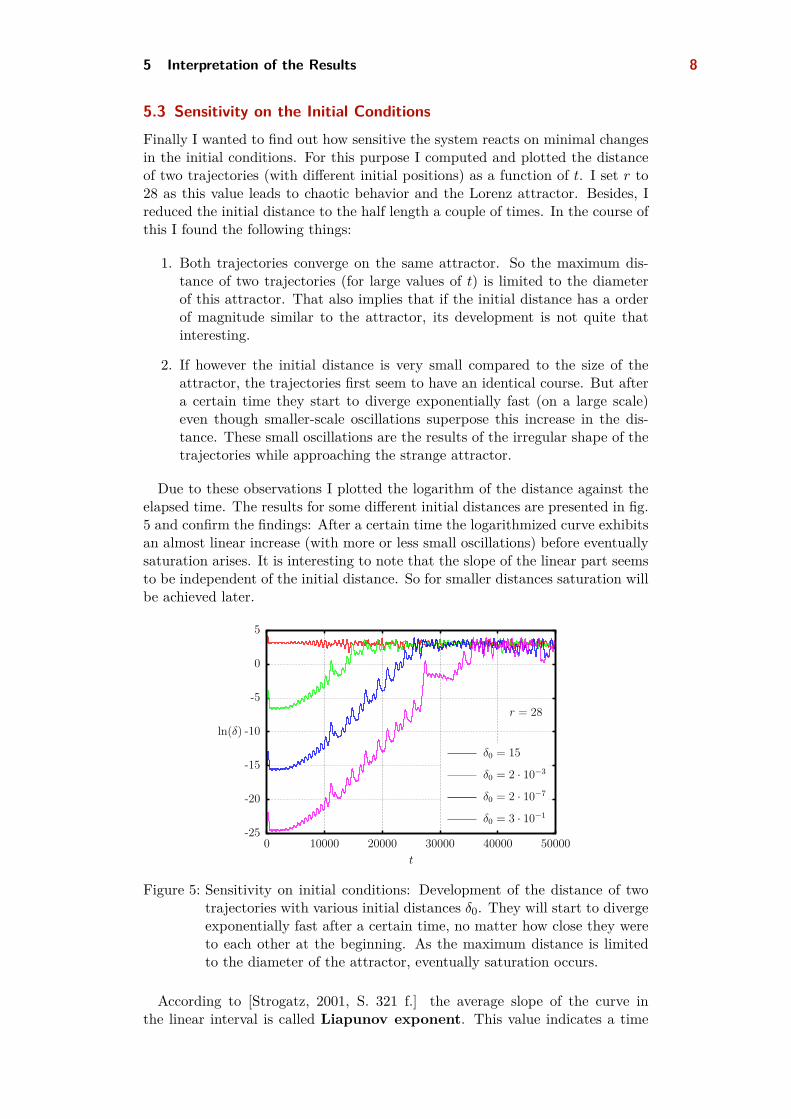
5.3 Sensitivity on the Initial ConditionsFinally I wanted to find out how sensitive the system reacts on minimal changesin the initial conditions. For this purpose I computed and plotted the distanceof two trajectories (with different initial positions) as a function of t. I set r to28 as this value leads to chaotic behavior and the Lorenz attractor. Besides, Ireduced the initial distance to the half length a couple of times. In the course ofthis I found the following things:

1. Both trajectories converge on the same attractor. So the maximum dis-tance of two trajectories (for large values of t) is limited to the diameterof this attractor. That also implies that if the initial distance has a orderof magnitude similar to the attractor, its development is not quite thatinteresting.

2. If however the initial distance is very small compared to the size of theattractor, the trajectories first seem to have an identical course. But aftera certain time they start to diverge exponentially fast (on a large scale)even though smaller-scale oscillations superpose this increase in the dis-tance. These small oscillations are the results of the irregular shape of thetrajectories while approaching the strange attractor.

Due to these observations I plotted the logarithm of the distance against theelapsed time. The results for some different initial distances are presented in fig.5 and confirm the findings: After a certain time the logarithmized curve exhibitsan almost linear increase (with more or less small oscillations) before eventuallysaturation arises. It is interesting to note that the slope of the linear part seemsto be independent of the initial distance. So for smaller distances saturation willbe achieved later.

-25

-20

-15

-10

-5

0

5

0 10000 20000 30000 40000 50000

ln(δ)

t

r = 28

δ0 = 15

δ0 = 2 · 10−3

δ0 = 2 · 10−7

δ0 = 3 · 10−1

Figure 5: Sensitivity on initial conditions: Development of the distance of twotrajectories with various initial distances δ0. They will start to divergeexponentially fast after a certain time, no matter how close they wereto each other at the beginning. As the maximum distance is limitedto the diameter of the attractor, eventually saturation occurs.

According to [Strogatz, 2001, S. 321 f.] the average slope of the curve inthe linear interval is called Liapunov exponent. This value indicates a time


horizon beyond which prediction breaks down. In real studies it is impossibleto determine the initial conditions exactly, so for chaotic systems one cannotpredict future states precisely. If the time t becomes big enough, the predictedbehavior will differ completely from the real behavior.So the system reacts extremely sensitive on small changes in the initial con-

ditions. For a better illustration of this I created one more plot (see fig. 6).Therefor I simulated the Lorenz system for a couple of initial positions that werefairly close to each other (average distance of around 10−3). Then I plotted thedistribution of the the resulting trajectory positions for several values of t. Itbecomes clear that they first remain close to each other but after some timediverge exponentially fast so that they are scattered over the whole attractor fort > 30000.

-20 0 20 -200 2002040

t = 0

-20 0 20 -200 2002040

t = 17000

-20 0 20 -200 2002040

t = 20000

-20 0 20 -200 2002040

t = 36000

initial conditions:x0 = 1y0 = 1z0 = 1

xy

z

Figure 6: Divergence of trajectories with small initial distance. A red point in-dicates the position of one trajectory in the phase spase at the statedtime t. Although the initial distances were very small (around 10−3)the states in the phase space quickly spread on the whole attractorwhich is indicated by the green color.

References 10

ReferencesMaria Haase Rudolf Friedrich John Argyris, Gunter Faust. Die Erforschung des

Chaos. Springer, 2 edition, 2010.

Dieter Meschede. Gerthsen Physik. Springer-Verlag Berlin Heidelberg, 24 edition,2010.

Steven H. Strogatz. Nonlinear Dynamics and Chaos. Perseus Books Group,2001.

Daoqi Yang. C++ And Object-Oriented Numeric Computing for Scientists andEngineers. Springer, 2000.

simulation and analysis of the lorenz...

Documents