shock tube design and the kinematics of the hybrid iii
TRANSCRIPT
SHOCK TUBE DESIGN AND THE KINEMATICS OF THE
HYBRID III DUMMY HEAD UNDER SHOCK WAVES OF
BLAST
A Thesis Submitted to the Graduate Faculty
Of the North Dakota State University
Of Agriculture and Applied Science
By
Ka-Ho Derek Leung
In Partial Fulfillment of the Requirements For the Degree of
MASTER OF SCIENCE
Major Department: Mechanical Engineering
April 2012
Fargo, North Dakota

ii
North Dakota State University Graduate School Title
Shock Tube Design and the Kinematics of the Hybrid III Dummy Head under
Shock Waves of Blast By
Ka-Ho Derek Leung
The Supervisory Committee certifies that this disquisition complies with North Dakota State University’s regulations and meets the accepted standards for the degree of
MASTER OF SCIENCE
SUPERVISORY COMMITTEE:
Dr. Ghodrat Karami
Chair
Dr. Mariusz Ziejewski
Dr. Fardad Azarmi
Dr. Benton Duncan
Approved:
April 2012
Dr. Alan Kallmeyer
Department Chair
iii
ABSTRACT
Traumatic brain injury (TBI) is one of the most common injuries to soldiers in
warfare today. A TBI occurs when the human brain is damaged by a sudden force
coming from the environment. Blasts created by improvised explosive devices
(IEDs) can cause damage to other human body parts including lungs, bowels, and
any other air-containing organs. In this study, a blast shock tube was constructed
for use with a Hybrid III dummy head model for mimicking the blasting scenario to
obtain mechanical behavior data from when the generated compressed air is
released from the blast shock tube. The acceleration based on the standoff
distance of the Hybrid III head could be found. A simple model was established for
finite element (FE) analysis. The results showed that the closer the dummy head
was to the shock tube opening and the higher the pressure pulse being used and
more.

iv
ACKNOWLEDGEMENTS
I would like to thank my advisors, Dr. Ghodrat Karami and Dr. Mariusz
Ziejewski, for supporting and guiding me through my Master’s Degree program. I
would also like to thank Dr. Fardad Azarmi and Dr. Benton Duncan for serving as
the Supervisory Committee Members for my research, Dr. Majura Selekwa for his
support on the data acquisition system setup and a special thanks to my
colleagues for their help, support, and recommendations leading to the completion
of this research.
The research was supported financially by the U.S. Army; therefore I would
also like to thank the United States Army for financially supporting the research,
and the Mechanical Engineering Department, North Dakota State University for
providing me with financial support during the time that I was in the Master’s
Degree program. Finally, I want to thank my family and my friends for encouraging
me, and lifting me up every time I had any type of difficulties.

v
TABLE OF CONTENTS
ABSTRACT ............................................................................................................. iii
ACKNOWLEDGEMENTS .......................................................................................iv
LIST OF TABLES ................................................................................................... vii
LIST OF FIGURES ................................................................................................ viii
CHAPTER 1. INTRODUCTION AND RESEARCH OBJECTIVES ......................... 1
1.1. Explosive Materials .................................................................................... 2
1.2. Blast Injuries Classification ........................................................................ 3
1.3. Blast Conditions ......................................................................................... 5
1.4. Traumatic Brain Injury ................................................................................ 9
1.5 Research Objectives ................................................................................ 10
CHAPTER 2. A REVIEW OF BLAST SIMULATION BY SHOCK TUBE AND NUMERICAL COMPUTATION .............................................................................. 11
2.1. Blast Simulation Experiments .................................................................. 11
2.2. Finite Element Analysis Simulations ........................................................ 14
CHAPTER 3. DESIGN AND ELEMENTS OF THE SHOCK TUBE AND EXPERIMENTAL PROCEDURE ........................................................................... 27
3.1. Experimental Setup .................................................................................. 27
3.1.1. Air Compressor ................................................................................... 27
3.1.2. Driver Section ..................................................................................... 28
3.1.3. Solenoid-Controlled Pneumatic-Actuated Butterfly Valve ................... 29
3.1.4. Testing Sections ................................................................................. 30
3.1.5. Data Acquisition .................................................................................. 31
3.2. Dummy Head/Neck .................................................................................. 32
3.3. High Speed Camera/Computer/Motion Studio ......................................... 33

vi
3.4. Experimental Procedure ........................................................................... 34
CHAPTER 4. EXPERIMENTAL RESULTS AND DISCUSSIONS ........................ 36
4.1. Tracking Results ...................................................................................... 38
4.2. Accelerometers Results ........................................................................... 50
CHAPTER 5. FINITE ELEMENT ANALYSIS OF THE SHOCK TUBE FLOW ...... 55
5.1. LS-DYNA FE Software ............................................................................. 55
5.1.1. Preliminary Shock Tube Model ........................................................ 55
5.1.2. Condition Setups .............................................................................. 56
5.1.3. Numerical Results on the Preliminary Model ................................... 57
5.1.4. Validation of existing model using FEM ........................................... 59
5.1.5. Validation Results ............................................................................ 60
5.1.6. Modified Model for the Blast Shock Tube......................................... 62
5.1.7. Results on the New Model ............................................................... 62
5.2. Computational Fluid Dynamics (ANSYS – CFX) ...................................... 68
5.2.1. Air Flow Model ................................................................................. 68
5.2.2. Boundary Conditions for the Air Flow Model .................................... 70
5.2.3. Pressure Distribution inside the Shock Tube ................................... 71
CHAPTER 6. CONCLUSIONS ............................................................................. 77
CHAPTER 7. RECOMMENDATIONS FOR FUTURE STUDIES ......................... 81
REFERENCES CITED .......................................................................................... 83

vii
LIST OF TABLES
Table Page
1-1: Mechanisms of Blast Injury (WebRef2, 2012). ............................................. 4
1-2: Correlation between damage and overpressure (Kinney and Graham, 1985). ................................................................................... 5
4-1: Maximum velocities of the dummy head based on three tests on each scenario. ..................................................................................................... 47
4-2: Maximum accelerations of the dummy head based on three tests on each scenario...................................................................... 48
4-3: Average maximum acceleration of the dummy head in x-direction. ........................................................................................... 52
4-4: Average maximum acceleration of the dummy head in y-direction (filtered). ............................................................................. 52
5-1: Maximum accelerations on different spots of the head model. .................. 59
5-2: Maximum velocities from the modified shock tube model and head. ................................................................................................ 63
5-3: Maximum velocities due to different pressure pulses on various spots of the head model. .................................................................. 64
5-4: Maximum pressure based on different pressure pulses on different spots of the head model. .................................................... 67

viii
LIST OF FIGURES
Figure Page
1-1: A classic Pressure vs. Time curve at a point at the scene (Brooks et al., 1997). ......................................................................... 7
1-2: The relationship between peak overpressure and standoff distance when 10 kg of TNT is being used (Brooks et al., 1997). ................................................................................................ 8
2-1: Pressure distributions at different locations in the shock tube (Segars et al., 2008). ...................................................................... 12
2-2: Results based on different situations (Leonardi et al., 2011). .................... 14
2-3: The 2D model of shock tube for the sandwich panel experiment (Tan et al., 2010). ............................................................................ 16
2-4: Comparison between FEA results and ConWeb (Tan et al., 2010). .............................................................................................. 16
2-5: Different views on panel's deformation due to the blast as a) side view b) front view of the sandwich (Tan et al., 2010). .............. 17
2-6: Meshed model consists of explosive, air, and rolled homogeneous armor plate (Chafi et al., 2009). ............................... 18
2-7: Comparison between the experiment result (Boyer, 1960) and the numerical result (Chafi et al., 2009). ......................................... 19
2-8: Pressure distribution based on distance from explosion while different amounts of TNT are being used (Chafi et al., 2009). .............................................................................................. 20
2-9: Different views of the head model showing different parts of the human head (Chafi et al., 2010)...................................................... 21
2-10: Pressure distribution of the model at different time (Chafi et al., 2010). ........................................................................................... 23
2-11: Average ICP over time when three different amounts of high explosives are being used (Chafi et al., 2010). ............................. 23
ix
2-12: The head and neck model for the simulation with the use of springs and dampers (Dirisala et al., 2011). ................................. 24
2-13: Pressure distribution over time on the head model when different damping coefficients are used while a) is using an elastic neck and b) is using a viscoelastic neck. The experimental results are from Nahum et al. in 1977 (Dirisala et al., 2011). .................................................................... 25
3-1: An overall look at the experimental setup. ................................................. 27
3-2: The air storage section (driver section) and the two stands holding the shock tube. ................................................................... 28
3-3: The actual Hybrid III 50th Percentile Male Crash Test Dummy Head/Neck.32
3-4: The Hybrid III Dummy Head with the reference point from the camera view. ................................................................................... 33
4-1: The velocity plot with different pressure pulses being used over time. ................................................................................................ 37
4-2: Rippling of the rubber face during testing at different time. ........................ 38
4-3: Acceleration over time plot with three different pressure pulses when the reference point on the dummy head is 5 inches away from the shock tube opening. ................................................ 39
4-4: Acceleration over time plot with only 50 and 75 psi pressure pulses. ............................................................................................ 40
4-5: Velocity curves over time based on different placements of the head while 50 psi pressure pulse was used. ................................... 41
4-6: Velocity curves based on different placements of the dummy head over time when pressure pulse is set to be 75 psi. ................ 42
4-7: Velocity curves based on different placements of the dummy head over time with 100 psi pressure pulse being used. ................ 43
4-8: Moving average trend lines with 4 periods for acceleration curves over time when 50 psi pressure pulse while the head is placed at 3 different locations (reference point is 5, 7.5, 10 inches away from the shock tube opening). .................... 44

x
4-9: Acceleration curves based on different placements of the dummy head with 75 psi pressure pulse being used. ..................... 45
4-10: Acceleration curves based on different placements of the dummy head when 100 psi pressure pulse is used. ...................... 46
4-11: Maximum velocity of the dummy head based on different standoff distance (placement). ...................................................... 49
4-12: Maximum acceleration of the dummy head based on different standoff distance. ........................................................................................ 49
4-13: Moving average trend lines with 200 periods for accelerations curves with 50 psi pressure pulse is used when the reference point on the dummy head is 5 inches away from the shock tube opening. ........................................................ 50
4-14: Acceleration curves with 50 psi pressure pulse used while the dummy head was set 10 inches away from the shock tube opening. ................................................................................ 51
4-15: Maximum acceleration of the dummy head based on standoff distance in x-direction. ........................................................................................ 53
4-16: Maximum acceleration of the dummy head based on standoff distance in y-direction. ........................................................................................ 54
5-1: Preliminary shock tube model in LS-DYNA. ............................................... 56
5-2: a) Initial stage of the model, b) valve is turned 90 degrees. ....................... 57
5-3: Flow velocity with 100 psi pressure pulse. ................................................. 57
5-4: Acceleration of the head model when it is placed 5 inches away from the shock tube opening while 100 psi pressure pulse is used. .................................................................................. 58
5-5: Shock Tube by J. M. Varas et al. ............................................................... 59
5-6: Experimental results from Varas' shock tube (2011). ................................. 60
5-7: Pressure plot based on different areas of the head model. ........................ 61
5-8: Modified shock tube model for simulation. ................................................. 62
xi
5-9: Velocity distribution of the head model based on different pressure pulses (50, 75, and 100 psi) when the middle point of the head is 5 inches away from the shock tube opening. .......................................................................................... 63
5-10: Acceleration plot with 50 psi pressure pulse with 5 inches head placement. ..................................................................................... 64
5-11: Acceleration based on pressure pulses on different spots of the head. ....................................................................................... 65
5-12: Pressure plot with 50 psi pressure pulse on different places of the head model. ............................................................................ 66
5-13: Pressure on front area of the head with different pressure pulses. ........................................................................................... 66
5-14: Maximum pressure on different spots of the dummy head based on different pressure pulses being used. ............................ 68
5-15: Shock tube model used for CFX simulation. ............................................ 69
5-16: Shock tube model along with conditions applied. ..................................... 70
5-17: Pressure distributions at t = a) 0, b) 3, c) 6, d) 9, e) 12, f) 15, g) 18, h) 20 ms. ................................................................................. 73
5-18: Pressure vs. Time plot at 5 different spots in the system. ........................ 74
5-19: Velocity vs. Time plot at five different spots in the system. ...................... 76

1
CHAPTER 1. INTRODUCTION AND RESEARCH
OBJECTIVES
In the field of combat, high pressure blasts created by improvised
explosive devices (IEDs) are always a threat and are the major cause of
traumatic brain injuries (TBIs). Therefore traumatic brain injuries caused by IEDs
are called ‘signature wounds’ of any wars today (Magnuson, 2010).
TBI is one of the most common injuries happening to soldiers today, and
research on diagnosing TBIs is one of the major components for determining
treatments for them, as well as means for preventing them. TBI occurs when a
human brain is hit by a sudden force, acceleration, or deceleration coming from
the environment. Acceleration is the most important engineering parameter that
leads to brain injury, as it shows the change of velocity depending on time. As a
result, the severity of the brain injury is characterized based on the acceleration
of the human head, while the acceleration is determined by the combination of
three linear acceleration components and three angular acceleration components
(Ziejewski et al., 2007).
According to the Department of Veterans Affairs in 2007, there were about
1800 troops with TBIs. Neurologists have estimated that roughly 30 percent of
the troops that are at risk to TBI may also be at high risk to get any type of
neurological disorder after four months or longer of combat, due to the blast
conditions coming from the explosives (Glasser, 2007).
2
It is estimated that 19.5% of all U.S. troops have symptoms related to
blast induced traumatic brain injury (bTBI), which is possibly the cause of the
neurological disorders like migraine headaches, insomnia, or dizziness (Helmick
et al., 2006, Tanielian & Jaycox, 2008, Anderson, 2008, Cifu et al., 2009)
1.1. Explosive Materials
Explosives are one of the most common weapons used in warfare today.
They are extremely dangerous due to their explosions and blast radius. A
description of the mechanism of the explosive is that it is simply the energy of
motion. For example, the explosive consisting of trinitrotoluene (TNT), with
proper handlers, is an object that has chemical potential energy. When the TNT
is detonated, the potential energy is turned into kinetic energy and motion is
created. At the same time, blast is formed when the motion of air starts. Other
than the blast, thermal energy is created due to the blast, which involves a high
velocity change of the air. Such a process is considered to be exothermic, which
is an energy releasing reaction from the system. Most of the time, this process is
in the form of heat, light, or sound (WebRef3, 2012).
The explosives are classified as low-order and high-order. The low-order
explosives create explosions that are supposedly slower than Mach 1, which is
the speed of sound. The low-order explosives produce a subsonic wave, and the
high-order explosives produce a supersonic wave, which is an over-
pressurization wave that the low-order explosives would never have (WebRef3,
2012).
3
In the battle field, military purposed explosives are all high-order
explosives, while the terrorists would use high-order explosives, low-order
explosives, or the combination of both (WebRef3, 2012).
1.2. Blast Injuries Classification
Blast injuries can be classified into the four major mechanisms of primary,
secondary, tertiary, and quaternary. The blast injuries classifications are based
on the anatomical and physiological changes from the body being impacted by
any external forces (WebRef2, 2012).
Primary blast injuries are caused by the impact of the shock wave to our
human bodies. In other words, the injuries are caused when human body is
being hit by the blast that changes the atmospheric pressure of any medium
(Ziejewski et al., 2007), and may occur without any visible external signs. These
Injuries mostly occur in specific organs that contain air, such as lungs and
bowels. Other than those organs, it is believed that the shock wave can also
damage the human brain (Brooks et al., 1997).
Secondary blast injuries are caused by the impact of fragments and any
objects within the bombing device that are accelerated by the blast. Injuries in
this classification can be categorized as penetrating or non-penetrating,
depending on the injuries (Brooks et al., 1997).
Tertiary blast injuries are caused by the sudden acceleration of the human
body by the blast which then hits the ground or any rigid objects leading to any
tearing of body parts or tissue (Brooks et al., 1997). The fourth type of blast
injuries mechanism is the quaternary, which are related to burns due to the

4
explosion, the combustion of the environment, or any dangerous gas that is not
related to any of the other three classifications of blast injuries (Brooks et al.,
1997). The following is a table of mechanisms for the blast injury.
Category Characteristics Body Part Affected
Types of Injuries
Primary Unique to HE, results from the impact of the over-pressurization wave with body surfaces.
Gas filled structures are most susceptible – lungs, GI tract, and middle ear.
Blast lung (pulmonary barotraumas) TM rupture and middle ear damage Abdominal hemorrhage and perforation – Globe (eye) rupture – Concussion (TBI without physical signs of head injury)
Secondary Results from flying debris and bomb fragments.
Any body part may be affected.
Penetrating ballistic (fragmentation) or blunt injuries Eye penetration (can be occult)
Tertiary Results from individuals being thrown by the blast wind.
Any body part may be affected.
Fracture and traumatic amputation Closed and open brain injury
Quater nary All explosion-related injuries, illnesses, or diseases not due to primary, secondary, or tertiary mechanisms. Includes exacerbation or complications of existing conditions.
Any body part may be affected.
Burns (flash, partial, and full thickness) Crush injuries Closed and open brain injury Asthma, COPD, or other breathing problems from dust, smoke, or toxic fumes Angina Hyperglycemia, hypertension
Table 1-1: Mechanisms of Blast Injury (WebRef2, 2012).

5
Based on the level of pressure of the blast, it causes different kinds
damage to the human body. The following is a brief table showing the damage
caused by different levels of blast overpressure (Kinney and Graham, 1985).
Type of damage Overpressure (psi)
Personnel knocked down ~1-1.5
Eardrum rupture ~5-15
Lung damage ~29-75
Lethality ~100-220
Table 1-2: Correlation between damage and overpressure (Kinney and Graham,
1985).
1.3. Blast Conditions
A blast can be created by using several methods. One method would be
to create an explosive, and another common method would be to construct a
shock tube, which involves the work of compressed gas. In the battlefield,
blasts are found mostly by the detonation of the explosive materials. The
strength of the blast caused by the explosive materials depending on two major
elements. One of the two elements is the explosive charge weight, which is
measured based on the identical amount of TNT. The other element is the
standoff distance between the explosive and the object that is receiving the blast
that is created by the explosive (Ziejewski et al., 2007).
A shock tube would be a better or safer way to create shock waves versus
making an explosive, which would be more dangerous. There are two main
sections of a shock tube: 1) the driver section and 2) the driven section. The

6
high pressure gas is usually stored in the driver section of the shock tube while
the driven section usually contains low pressure gas, or ambient environment.
The two sections are separated by a component, which can be a rupture disk or
a butterfly valve that can be opened quickly, depending on the preference.
As the separating component is gone or opened quickly, the high pressure
gas in the driver section flows into the driven section. Such operation finally
creates the blast condition as the gas in the driver section is going into the driven
section with an extremely high velocity. The high pressure gas ends up having
the same pressure as the low pressure gas after a short period of time.
The driven section can sometimes be called the chamber section,
because there is usually a test chamber in the section. Testing devices can be
placed in the chamber section so data can be obtained by performing the test.
Some examples of these testing devices would be any load cells,
accelerometers, air velocity transducers, pressure sensors or any other devices.
After the explosion occurs, a high pressure is formed in an extremely short
period of time. After that, the high pressure generated from the explosion travels
outward as a wave with an extremely high velocity. The high pressure was then
lowered quickly due to the surrounding condition, and finally returned back to its
normal condition. This was the process of the shock wave, as shown as Figure
1-1 (Brooks et al., 1997).
7
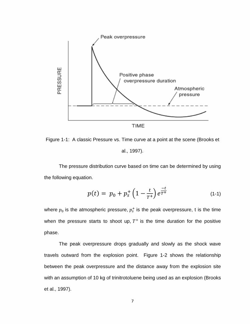
Figure 1-1: A classic Pressure vs. Time curve at a point at the scene (Brooks et
al., 1997).
The pressure distribution curve based on time can be determined by using
the following equation.
���� � �� � � �1 ���� �
���� (1-1)
where �� is the atmospheric pressure, � is the peak overpressure, t is the time
when the pressure starts to shoot up, � is the time duration for the positive
phase.
The peak overpressure drops gradually and slowly as the shock wave
travels outward from the explosion point. Figure 1-2 shows the relationship
between the peak overpressure and the distance away from the explosion site
with an assumption of 10 kg of trinitrotoluene being used as an explosion (Brooks
et al., 1997).

8
Described as a danger to the human body, a powerful explosive would
generate blast waves of high pressure at a velocity of about 1600 ft/s from the
explosive and with a radius of a few hundred yards. The blast wave has two
different parts that cause damage to the human body: 1) the wave that causes
the positive phase overpressure, 2) after the first wave, as the air or any medium
is being forced hard, the vacuum space is created. The vacuum space is then
filled up with air and this causes high pressure again, which represents the
negative phase of overpressure. These sudden changes of pressure are leading
to the neurological injury, as traumatic brain injury would be part of (Glasser,
2007).
Figure 1-2: The relationship between peak overpressure and standoff distance
when 10 kg of TNT is being used (Brooks et al., 1997).
9
1.4. Traumatic Brain Injury
This study is related to TBIs caused by primary blasts. Recently, there
has been an increasing amount of research on TBIs as they are still a major
concern for the U.S. Army branches. A TBI occurs when a blast wave hits a
human head, causing a sudden acceleration of the head, leading to the brain
responding separately to the sudden environment as the skull and the brain have
different material properties. Brain tissues are first compressed then impacted
against the skull and the brain tissues expand/compress over and over again
inside the skull, and such movement causes void and destruction to the brain
tissues (Ziejewski et al., 2007).
According to the National Institute of Neurological Disorders and Stroke
(NINDS), a person with a mild Traumatic Brain Injury (mTBI) may remain
conscious, or lose consciousness for a few seconds to minutes. Besides losing
consciousness, other symptoms of mTBI include confusion, dizziness, and
blurred vision. When a person has a moderate, or severe TBI, he/she may
experience the same symptoms as a mTBI, but also seizures, loss of
coordination, agitation and more (WebRef4, 2012). Besides injuring human
heads, TBIs also have a negative impact on the economy. In just the year 2000,
TBIs cost the U.S. national economy about 60 billion dollars (Finkelstein and
Corso et al., 2006), while the National Centers for Disease Control and
Prevention (CDC) estimated a cost of about 76.5 billion dollars in 2000 which
included the direct medical costs and the indirect costs such as lost of
productivity in 2000.

10
1.5 Research Objectives
The objective of this research was to determine the motion of the Hybrid III
Dummy Head when it is hit by the pressure pulse generated by the blast shock
tube. This research is divided into three major parts.
The first part of the research was the construction of a blast shock tube
and the stands along with a rail system for the dummy head. The shock tube was
used to simulate the blast similar to the blast condition created by the explosions
of explosive materials. The assembling of stands and rail system for the dummy
head was for the purpose of allowing the dummy head to slide through in a uni-
direction when being hit by the pressure pulse generated by the blast shock tube.
The second part of the work was to measure the linear velocity and
acceleration of the Hybrid III Dummy Head when it was subjected to various
pressure pulses generated by the shock tube. The measurement of the velocity
and acceleration of the dummy head was to determine the damage that the
dummy head might experience, as a TBI is caused by the sudden acceleration of
a human head.
The third part of this research was to determine the relationships between
the linear velocity, acceleration of the head model and the pressure pulse using
finite element (FE) analysis, as well as the relationship between the pressure
pulse and the standoff distance. The FE analysis approach helped in
understanding the mechanism of the blast on the head model that was similar to
the experiments. The use of FE analysis software could have also helped
determine the reaction of the air flowing inside the chamber section of the shock
tube.

11
CHAPTER 2. A REVIEW OF BLAST SIMULATION BY
SHOCK TUBE AND NUMERICAL COMPUTATION
This chapter describes some past studies that are related to this research.
Some of the studies are about the construction of the shock tube, while others
involve the reactions that have occurred in rat brains under a blast, or how the
pressure has changed in a specific area inside the shock tube over a period of
time. Other than experimental research, numerical research has also been
conducted by using head models for simulating the reactions to the human head.
These studies had some reasonable results and are therefore useful references
for other researchers.
2.1. Blast Simulation Experiments
The shock tube constructed by Ronald Segars and Marina Carboni at the
U.S. Army Natick Soldier Research Development and Engineering Center
(NSRDEC) showed important data on the differences when assorted test
materials were used (Segars et al., 2008). The testing materials for their
research include three different types of foams, Kevlar ® fabric, and aluminum
foil while all had different material properties. The shock tube was made of
stainless steel pipe with an inner diameter of 6.72 cm and an outer diameter of
7.28 cm, respectively. The driver section of the tube was 30.5 cm long while the
driven section was exactly 183 cm long. For each section of both, there were
two stainless steel flanges attached to each end. The yield strength of the used
tube was about 4000 psi, which was close to the pressure that the tube could

12
hold. There was also a total of five sensor taps used on the shock tube, for
finding the changes of the pressure at different spots inside the shock tube.
Placing multiple pressure sensors at different sections in the shock tube give out
different pressure distributions of the flow. Figure 2-1 shows a set of plots with
data obtained from the four pressure taps, P1 is for the flow in the tube wall by
the diaphragm, P2 is in the tube wall by the endplate, P3 measures the reflected
pressure at the endplate, and P4 measures the reflected pressure at the
recessed sensor.
Figure 2-1: Pressure distributions at different locations in the shock tube (Segars
et al., 2008).
13
A shock tube made by Leonardi et al. (2011) was used at Wayne State
University (WSU) to study the increases of intracranial pressure (ICP) due to
shockwaves. The shock waves were generated by using helium as the driven
gas, the shock tube had a total length of 272 inches, which included the 30
inches driver section and the 242 inches long driven section. To verify the
accuracy of the results in the case of using the in vivo method, 25 male Sprague-
Dawley rats were used in the experiment while guided cannula was placed inside
the rats’ skulls. The rats were then placed in a soft hold inside the shock tube so
they would face the shockwaves once the test is run. Unlike the other shock
tubes, the one at WSU had a transparent pipe at one end of the metal pipe. The
purpose of the transparent pipe was to make the full process of the experiment
visible, by human vision. By using a high speed camera, the researchers did not
have to stand by the opening of the shock tube. Similar to the other shock tube
experiments, this shock tube helped obtain the data of ICP over a short period of
time. There was a possibility that the ICP could change due to how the cannula
was sealed, Leonardi et al. (2011) tried different scenarios when the cannula was
unsealed, partially sealed, or fully sealed. Figure 2-2 shows the difference
between the different situations.
The results show that the incident shockwave overpressure had the lowest
peak overpressure while the totally sealed cannula had the highest peak
overpressure. Overall, the pressure was the highest when the cannula was
partially sealed. Negative pressure occurred for all the cases when the time got
to roughly 18.5 ms.

14
Figure 2-2: Results based on different situations (Leonardi et al., 2011).
2.2. Finite Element Analysis Simulations
FE analysis is a powerful tool for studying air blast and TBIs. Yet the
accuracy of the results from these simulations is highly dependent on the
accuracy of the model (Chafi et al., 2010). This includes material properties for
different parts of the model, geometry of the model, and conditions related to the
situation of the scene. Finite element analysis (FEA) can be used to analyze the
stress and displacement of the head model by using LS-DYNA. It can also help
in determining the reaction of the air flow, the air flow velocity, or the stagnation
pressure by using computational fluid dynamics (CFD).
A simple blast model usually involves the use of Arbitrary Lagrangian
Eulerian (ALE) elements for the explosive/TNT charger and the surrounding
environment/air while the detonation of the TNT is defined by using the Jones-
15
Wilkins-Lee (JWL) equation of state (EOS). The parameters for that specific
equation were estimated by Dobratz in 1985.
� � � �1 ����� ����� � � �1 �
���� ����� � ��� (2)
� !"! (3)
where p is the pressure, #� is the initial density of TNT, # is the density of the
detonation gas, A, B, R1, R2, ω are the parameters for the JWL equation, and E
represents the internal energy of the detonation.
A recent research on shockwave hitting on a sandwich panel by using the
finite element method (FEM) was done by Tan et al. (2010). The objective of
their research was to determine the performances of sandwich circular panels
when different materials are used under the condition of blasting. The
performances of the sandwiches were compared to performances found by using
the monolithic solid circular plates. Finding that the results of the peak
transmitted overpressure, deflection of the panels, and the acceleration of the
sandwiches were less than the results for the monolithic solid plates. The
research showed that the performance of the materials on the shock tube
blasting condition was based on the material property, configuration, and mass
distribution. Figure 2-3 shows a cross-sectional sketch of a shock tube for the
sandwich panel experiment (Tan et al., 2010).
16
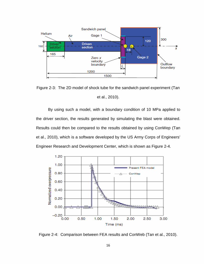
Figure 2-3: The 2D model of shock tube for the sandwich panel experiment (Tan
et al., 2010).
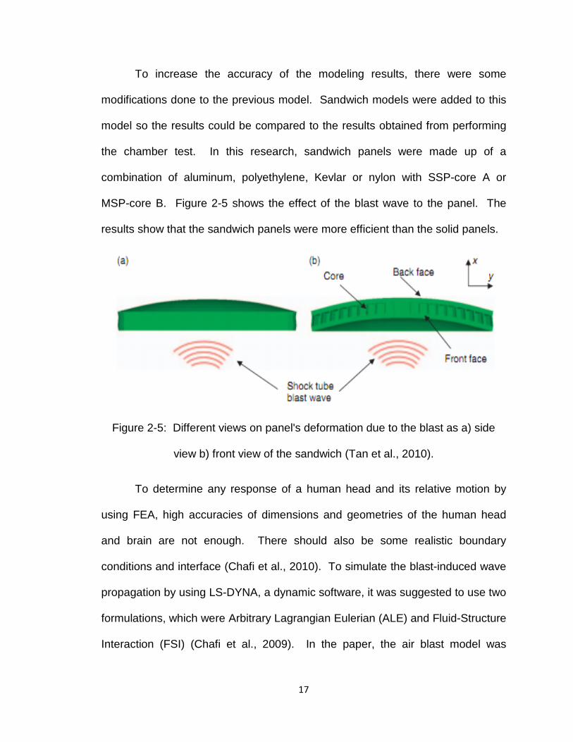
By using such a model, with a boundary condition of 10 MPa applied to
the driver section, the results generated by simulating the blast were obtained.
Results could then be compared to the results obtained by using ConWep (Tan
et al., 2010), which is a software developed by the US Army Corps of Engineers’
Engineer Research and Development Center, which is shown as Figure 2-4.
Figure 2-4: Comparison between FEA results and ConWeb (Tan et al., 2010).
17
To increase the accuracy of the modeling results, there were some
modifications done to the previous model. Sandwich models were added to this
model so the results could be compared to the results obtained from performing
the chamber test. In this research, sandwich panels were made up of a
combination of aluminum, polyethylene, Kevlar or nylon with SSP-core A or
MSP-core B. Figure 2-5 shows the effect of the blast wave to the panel. The
results show that the sandwich panels were more efficient than the solid panels.
Figure 2-5: Different views on panel's deformation due to the blast as a) side
view b) front view of the sandwich (Tan et al., 2010).
To determine any response of a human head and its relative motion by
using FEA, high accuracies of dimensions and geometries of the human head
and brain are not enough. There should also be some realistic boundary
conditions and interface (Chafi et al., 2010). To simulate the blast-induced wave
propagation by using LS-DYNA, a dynamic software, it was suggested to use two
formulations, which were Arbitrary Lagrangian Eulerian (ALE) and Fluid-Structure
Interaction (FSI) (Chafi et al., 2009). In the paper, the air blast model was

18
simulated by using multi-material ALE formulation as the ALE formulation. It was
also determined the effects from an actual explosive, because each element of
the model is to contain more than two different materials. FSI was to be
simulated for the interaction of some moving or fixed mesh using an ALE
formulation while the Lagrangian formulation was used for a deformable
structure. The air blast simulations were conducted by using LS-DYNA with the
usage of Eulerian Multi-Material, ALE formulations for the Navier-Stokes
equations and the Jones-Wilkins-Lee equation for the results of the explosion. In
the paper, the explosives used for simulations were C-4 and TNT and were
simulated in an open space so that it could simulate a battlefield scene. The
model is shown as Figure 2-6. The results for the simulation when C-4
explosives were used are plotted and compared to an experimental result
obtained by Boyer (1960). The plot shows that the results were comparable and
errors of the arrival time and peak pressure could be neglected.
Figure 2-6: Meshed model consists of explosive, air, and rolled homogeneous
armor plate (Chafi et al., 2009).
19
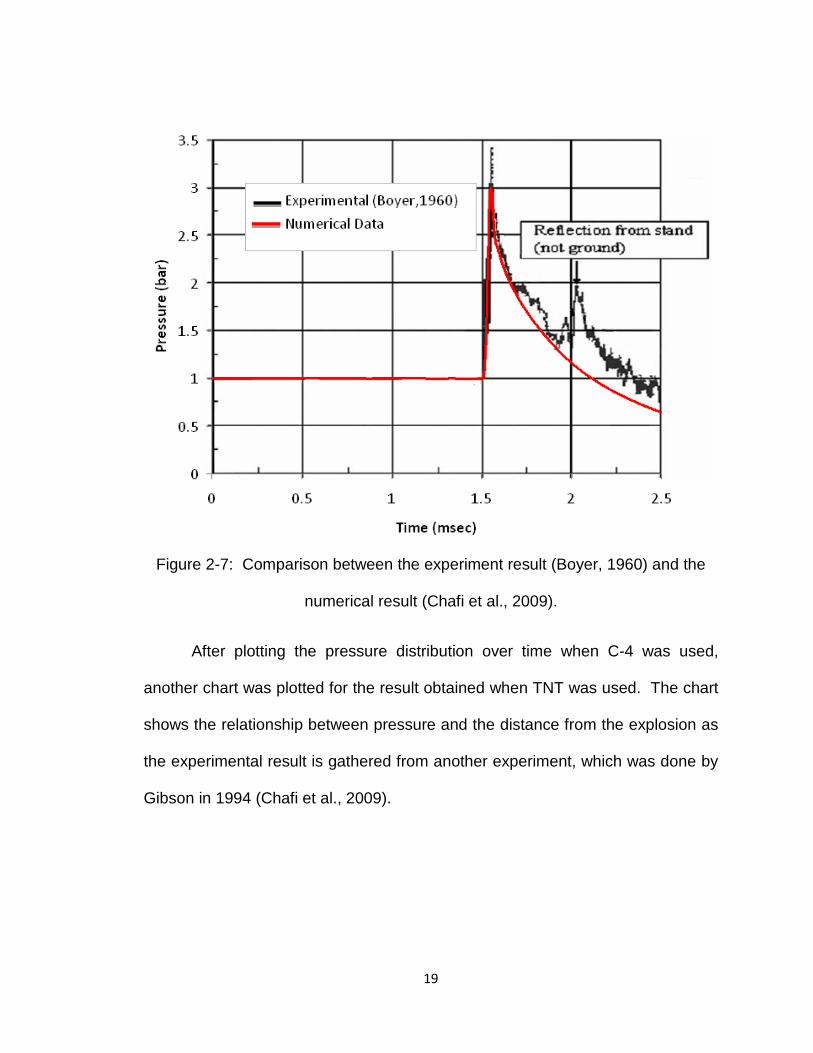
Figure 2-7: Comparison between the experiment result (Boyer, 1960) and the
numerical result (Chafi et al., 2009).
After plotting the pressure distribution over time when C-4 was used,
another chart was plotted for the result obtained when TNT was used. The chart
shows the relationship between pressure and the distance from the explosion as
the experimental result is gathered from another experiment, which was done by
Gibson in 1994 (Chafi et al., 2009).

20
Figure 2-8: Pressure distribution based on distance from explosion while
different amounts of TNT are being used (Chafi et al., 2009).
The results show that as the distance from the explosion became greater,
the pressure got lower. The errors between the experimental results (Gibson,
1994) and the numerical results (Chafi et al., 2009) less than 10% when 0.5, 1,
1.5, 2 pounds of TNT explosives were being used. This indicated that the cases
were in good agreements.
One research study was to assess the brain dynamic response when
being hit by blast pressure waves with the use of FEA. The 3-dimensional (3-D)
FE model was based on a highly detailed structure of a human head, which
included the human brain, falx and tentorium, dura mater, cerebrospinal fluid
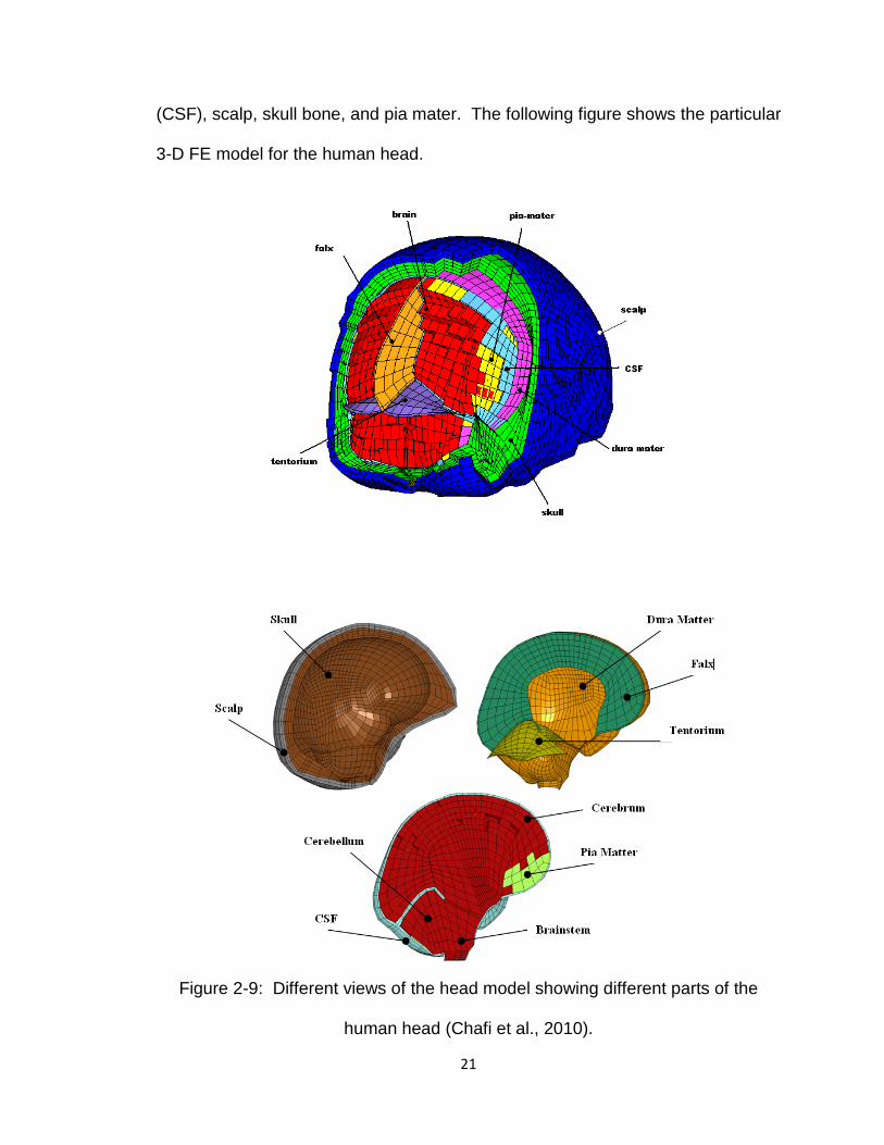
21
(CSF), scalp, skull bone, and pia mater. The following figure shows the particular
3-D FE model for the human head.
Figure 2-9: Different views of the head model showing different parts of the
human head (Chafi et al., 2010).
22
In a paper by Chafi (2010), the CSF was normally clear fluid that acted as
a cushion as it help protecting the brain and spine from injury and was modeled
with solid elements along with fluid-like property. The interface between the dura
and tentorium and the falx was defined to have a contact of tied node-to-surface
as these particular parts are physically attached to each other in human head. In
addition, the interface between the brain and membrane was modeled to have a
tied contact algorithm as loads could be transferred in both compression and
tension (Chafi et al., 2010). After modeling of the head, it used in the air-blast
simulation using the multi-material formulation used in the previous paper (Chafi
et al., 2009). In that case, the detonation was based on the explosion of high
explosives (HEs).
From the simulation, ICPs, maximum shear strains, and maximum shear
stresses were found through the time when the head human was hit by the blast
and the shock waves. The simulation was conducted several times which
included different amounts of the same explosive material. As expected, when
the amount of explosive material used, the higher the pressure, shear stresses,
and shear strain that occurred to the head model. The results showed that the
response happened to the head and lasted for about five miloseconds for such
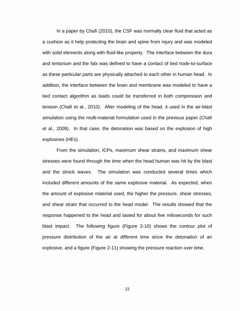
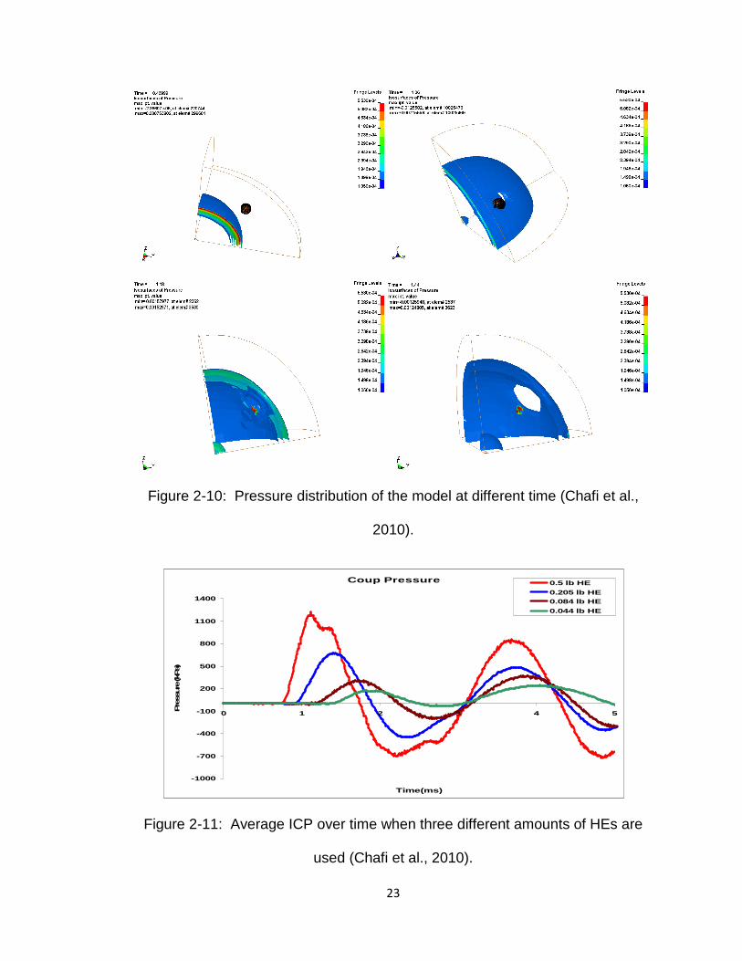
blast impact. The following figure (Figure 2-10) shows the contour plot of
pressure distribution of the air at different time since the detonation of an
explosive, and a figure (Figure 2-11) showing the pressure reaction over time.
23
Figure 2-10: Pressure distribution of the model at different time (Chafi et al.,
2010).
Figure 2-11: Average ICP over time when three different amounts of HEs are
used (Chafi et al., 2010).
Coup Pressure
-1000
-700
-400
-100
200
500
800
1100
1400
0 1 2 3 4 5
Time(ms)
Press
ure (kPa)
0.5 lb HE
0.205 lb HE0.084 lb HE
0.044 lb HE

24
In the work of Dirisala et al. (2011), an FE head model that cosisted of
almost all the parts of a human head was used. The geometry of the FE human
head model was based on magnetic resonance imaging (MRI) data with a total of
28,816 nodes and 19,589 8-node brick elements along with 5344 4-node shell
elements. The neck was created by using viscoelastic material by using discrete
elements while different damping coefficients were used to determine the
differences between each case. One end of the neck was assumed to be
connected to the head model while the other end was constrained. The specific
model is shown below. For the interfaces between the membranes in the head
model, node-to-surface and surface-to-surface tied based contact was used for
the simulations. The CSF was once again modeled to have some fluid-like
properties. The CSF and membranes used tied contact (Dirisala et al., 2011).
Figure 2-12: The head and neck model for the simulation with the use of springs
and dampers (Dirisala et al., 2011).
25
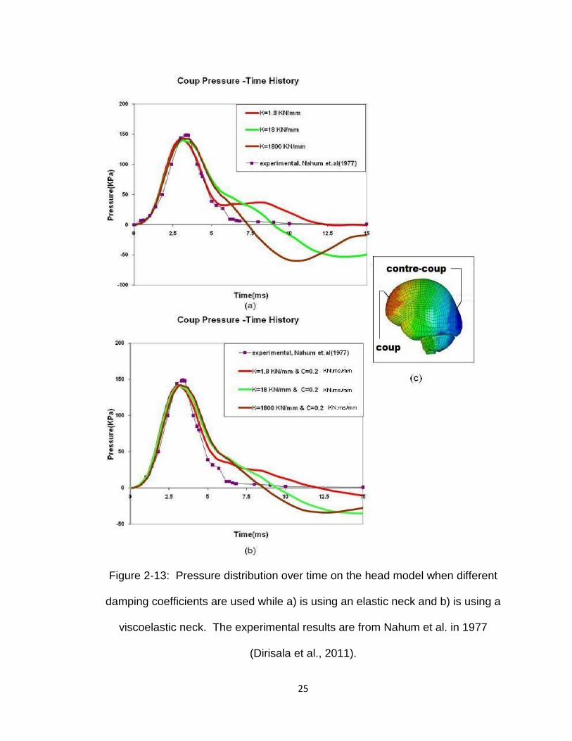
Figure 2-13: Pressure distribution over time on the head model when different
damping coefficients are used while a) is using an elastic neck and b) is using a
viscoelastic neck. The experimental results are from Nahum et al. in 1977
(Dirisala et al., 2011).
26
The results of the simulations show that the beginning stages of the
movement of the head are not much different from each other, but at the later
stages of the movement, the results showed that the intensity of the brain
response would be based on the neck damping coefficients. This meant that the
intensity of the brain response was going down when the damping coefficient of
the neck model was going up after the beginning stage of the movement of the
head (Dirisala et al., 2011).
27
CHAPTER 3. DESIGN AND ELEMENTS OF THE SHOCK
TUBE AND EXPERIMENTAL PROCEDURE
This chapter will describe the overall procedures for the experiment
presented in this paper, descriptions of the instruments used and the methods
used for acquiring the data.
3.1. Experimental Setup
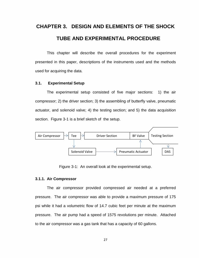
The experimental setup consisted of five major sections: 1) the air
compressor; 2) the driver section; 3) the assembling of butterfly valve, pneumatic
actuator, and solenoid valve; 4) the testing section; and 5) the data acquisition
section. Figure 3-1 is a brief sketch of the setup.
Figure 3-1: An overall look at the experimental setup.
3.1.1. Air Compressor
The air compressor provided compressed air needed at a preferred
pressure. The air compressor was able to provide a maximum pressure of 175
psi while it had a volumetric flow of 14.7 cubic feet per minute at the maximum
pressure. The air pump had a speed of 1575 revolutions per minute. Attached
to the air compressor was a gas tank that has a capacity of 60 gallons.
Testing Section Air Compressor Tee
Solenoid Valve Pneumatic Actuator
Driver Section BF Valve
DAS

28
3.1.2. Driver Section
In this section, compressed air was being transferred from the air
compressor. The pipe has an inner diameter of 8” while the thickness of the pipe
was 3/8”. One end of the tube was closed by welding a slab made of steel while
the other end was closed when the butterfly valve operated by the air
compressor. The air in this section supposedly compressed down to 170 psi,
which is about 11.568 atm. The steel pipe had minimum yield strength of 250
MPa, meaning that the internal pressure created by running the compressed air
into the steel pipe was safe. The driver pipe is shown below as Figure 3-2.
Figure 3-2: The air storage section (driver section) and the two stands holding
the shock tube.
29
The total length of the steel pipe between the closed end and the butterfly
valve was 289.5 inches. When adding the weight of the flanges, the total weight
of this section was then about 971 pounds. To lift the weight of this pipe of the
shock tube, there were two steel stands made and bolted to the flanges, which
were welded to the outer surface of the pipe. The frames were made by using
two inches by two inches square tubing, with a thickness of a quarter inch, and
angles that were welded to the frames so anchor bolts could go through the
angles and be bolted to the concrete floor.
3.1.3. Solenoid-Controlled Pneumatic-Actuated Butt erfly Valve
As described in Section 3.1, the valve assembling involved the assembling
of a butterfly valve, a pneumatic actuator, and a solenoid valve.
The high performance butterfly valve had the standard wafer pattern
meaning that there were only two holes that could be used for bolting the valve to
the flanges. The butterfly valve and the steel flanges all had the same 300 lbs
rating so they could handle a higher pressure and the valve size was 8 inches so
it matched the size of the pipe and the flanges. As the operating speed of the
butterfly valve was the priority of this experiment, a pneumatic actuator is chosen
instead of an electric actuator. An electric actuator would be more convenient,
but the fastest electric actuator for this size still needs about 10 seconds to
operate. A pneumatic actuator was the choice, therefore, as it could make the
butterfly valve open within a second. The selected pneumatic actuator was a
spring return type, meaning that when the actuator was filled with air, the butterfly
30
valve would begin to turn. When the valve was turned 90 degrees and closed,
the valve could spring back open by pressing a button.
Although a pneumatic actuator was a good choice and it did what it
needed to do, it did have some limitations during operations. The two major
limitations were the pressure range and the other is the temperature range. The
pressure range was between 40 and 120 psi, meaning that the experiment would
be fine when the operating pressure was not higher than 120 psi and not lower
than 40 psi when the operating temperature was between -4 and 176 degrees F.
The solenoid valve is an electro-mechanical valve that is mostly used for
experiments that involve air or fluids. The main purpose of the valve is to control
the air flow, which comes from the air compressor. By using the solenoid valve,
the compressed air used to operate the pneumatic actuator and the butterfly
valve can be released and the butterfly valve can then spring back to its original
position at high speed. The solenoid valve is designed to mount directly to the
pneumatic actuator so they can operate together. The solenoid valve has a flow
coefficient of 1.4. Similar to the pneumatic actuator, there are some limitations
for operating the solenoid valve. The operating temperature is between 20 and
125 degrees F, while the operating pressure is between 5 and 115 psi.
3.1.4. Testing Sections
This section was previously designed to have a removable cross-sectional
area chamber pipe larger than the driver pipe. When the chamber pipe was
used, the Hybrid III Dummy Head was constrained by four collars so that there
would be no movement on the base of the dummy head. The chamber pipe had
31
a length of 6 feet, an inner diameter of 15 inches and an outer diameter of 16
inches. One end of the chamber pipe was welded to the flow widener, and the
other end was open. There was also a hole with a diameter of 8 inches midway
through and at the bottom side of the pipe. The purpose of the hole was to allow
the dummy head to go through the hole and be placed inside the chamber.
When the testing chamber pipe was not attached to the stand, the
movement/reaction of the dummy head could be determined when the dummy
head was being hit by the pressure pulse and slides through the rail system.
The testing section had a length of 110 inches, and it had an estimated
weight of 600 lbs, including the flanges used to bolt the pipes together. To
withstand the weight, another stand with similar design to the stands was made
to hold the pressurized air storage pipe is made.
3.1.5. Data Acquisition
A data acquisition system was used to obtain useful data from any sensor
so that the data could be transferred to a computer. In this experiment, SCC-68
made by the National Instruments was the input/output connector block used.
Connected to the connector block by using wires, it helped connect the circuit
board to the power supply, and to the load cell sensor. The other side of the
connector block was connected to the circuit and to a computer by using a
specific cable and a card device.
To get the acceleration results, two accelerometers were used. Both
accelerometers were attached to a wood block, which was mounted to the load
cell by using bolts and nuts. The two accelerometers were used to measure the

32
accelerations of the dummy head in two different directions. One was the
direction of the head sliding through the rail, which was assumed to be x-
direction. The other accelerometer measured the acceleration of the dummy
head in its left/right direction, which assumed to be y-direction.
3.2. Dummy Head/Neck
The dummy head/neck used in the experiment was the Hybrid III 50th
Percentile Male Crash Test Dummy Head/Neck, and it was made by
Humanetics. The dummy itself is model used popularly in many different types of
crash tests and regulated by USA Code of Federal Regulations.
The skull and skull cap of the head model made of cast aluminum, while
the removable skin of the head made of vinyl (type of plastic). The neck
consisted of rubber and aluminum while there was a center cable inside the
neck, so that the model was able to have an accurate reaction due to any sudden
change of environment. Figure 3-3 shows the side view of the dummy
head/neck.
Figure 3-3: The actual Hybrid III 50th Percentile Male Crash Test Dummy
Head/Neck.

33
3.3. High Speed Camera/Computer/Motion Studio
Some of the experimental results were obtained by using the tracking
function from a high speed camera and Motion Studio software, which installed
into a computer. When the test was performed, the frames were captured by the
high speed camera and then transferred to the computer. The Motion Studio
software was able to analyze the work and useful data could then be obtained.
The camera was set 140 inches away from the center point of the shock tube
opening. To use the tracking function of the high speed camera, a reference
point was needed, and was selected to be the center of gravity point of the
dummy head as shown in Figure 3-4.
Figure 3-4: The Hybrid III Dummy Head with the reference point from the
camera view.
Reference Point

34
The Motion Studio software was to track the reference point while the
dummy head was hit by the blast and sliding through the rails. The test gave the
values of displacement, velocity, and acceleration in both the x and y directions.
3.4. Experimental Procedure
With there being many subsections for this experiment, the entire
procedure was somewhat complex. Before turning on the air compressor, the
hoses needed to be connected to the pipe, and the solenoid valve, and the air
compressor needed to be tight. The next step was to assure that the valve of the
air tank and one of the valves at the tee (In this case, the solenoid valve) were
open. Finally, the air compressor needed to be turned on so it could start
pumping air into the solenoid valve through the hose.
The maximum operating pressure was about 115 psi, and air was pumped
into the solenoid valve until the air pressure reached a preferred pressure that
was less than 115 psi. As the air pressure was increased, the butterfly valve
started turning, until it finally was at its closed position.
The next step was to close the opened valve and open the closed valve at
the tee so that the air could start getting pumped into the compressed air storage
section pipe. The air pressure inside the storage pipe was increased to about
100 psi, and could be checked by looking at the pressure gauge at the end of the
pipe. When the pressure got up to 100 psi, the air compressor could be turned
off and all the preparations were complete. The test was then ready to proceed.
With everything ready, the test began by pressing the red button on the
solenoid valve. Before running the test, the dummy head needed to be secured

35
correctly and ear plugs were needed as it was anticipated that the blast created
by using the shock tube would be extremely loud. By pressing the button, the air
controlling the pneumatic actuator and the butterfly valve were released and the
butterfly valve returned to its original opened position. By the time the butterfly
valve was opened, within less than a second, the compressed air inside the
driver pipe flowed through the valve and the air flowed into the chamber pipe.
Part of the air hit the dummy head, some air circulated inside the chamber pipe,
and the rest exited at the open end of the chamber pipe.

36
CHAPTER 4. EXPERIMENTAL RESULTS AND
DISCUSSIONS
There was a total of 27 tests performed and used for this research. The
first parameter to be considered was the bending movement of the dummy
head/neck that led to a change of the expected results. When the head/neck
bending backward, the change of the velocity was supposed to be slightly
increased so that the slope of the velocity curve was a little steeper than when
the head/neck was not bent. After the bending of the head/neck, it then bounced
back to the original position, which caused the dropping of the velocity or the
dropping of the change of the velocity. After the short period of time of bending
of the head/neck, the velocity curve starts going back up once again until the
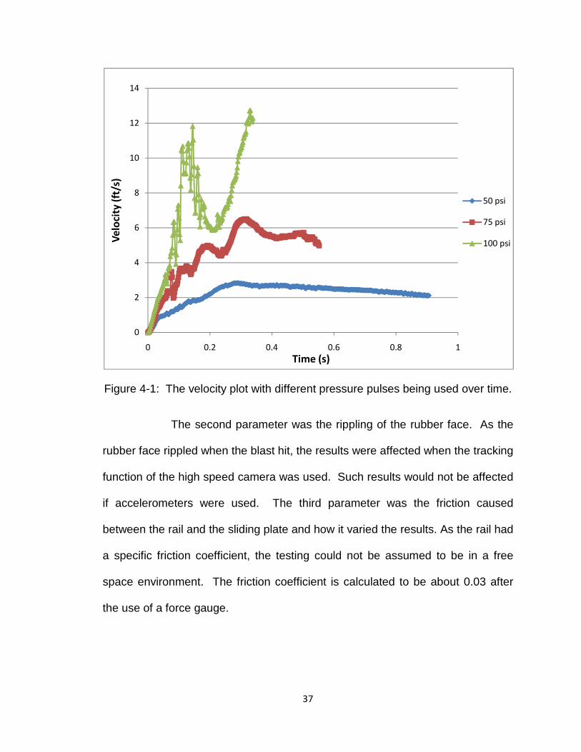
friction of the rail is slowed down the movement of the head/neck. Figure 4-1
shows the difference of velocity between different pressure pulses over a period
of time, while the reference point of the head/neck is set five inches away from
the shock tube opening. The velocity would be most affected when a higher
pressure pulse is used for testing. The higher the pressure pulse, the larger the
angle of the neck would be bent, plus the curve for lower pressure pulse would
be smoother than the curves for higher pressure pulses.
37
Figure 4-1: The velocity plot with different pressure pulses being used over time.
The second parameter was the rippling of the rubber face. As the
rubber face rippled when the blast hit, the results were affected when the tracking
function of the high speed camera was used. Such results would not be affected
if accelerometers were used. The third parameter was the friction caused
between the rail and the sliding plate and how it varied the results. As the rail had
a specific friction coefficient, the testing could not be assumed to be in a free
space environment. The friction coefficient is calculated to be about 0.03 after
the use of a force gauge.
0
2
4
6
8
10
12
14
0 0.2 0.4 0.6 0.8 1
Ve
loci
ty (
ft/s
)
Time (s)
50 psi
75 psi
100 psi

38
Figure 4-2: Rippling of the rubber face during testing at different time.
4.1. Tracking Results
The following plots (Figure 4-3) show the difference on linear acceleration
when different pressure pulses are used. The results are based on the data
obtained by using the high speed camera, with a unit of g that represented the
gravitational acceleration.

39
Figure 4-3: Acceleration over time plot with three different pressure pulses when
the reference point on the dummy head is 5 inches away from the shock tube
opening.
Figure 4-3 shows that the acceleration with a 100 psi pressure pulse had a
much higher magnitude than the other two curves, which were based on 50 psi
and 75 psi pressure pulses being used for testing. When the acceleration curve
for the 100 psi pressure taken away, there was not much change in acceleration
between the two cases as shown Figure 4-5.
-80
-60
-40
-20
0
20
40
60
80
100
0 0.05 0.1 0.15 0.2 0.25
Acc
ele
rati
on
(g
)
Time (s)
50 psi
75 psi
100 psi

40
Figure 4-4: Acceleration over time plot with only 50 and 75 psi pressure pulses.
The time plot shows that even without the acceleration curve of the 100
psi pressure pulse, the maximum acceleration based on the 75 psi pressure
pulse was about three times larger than the maximum acceleration based on the
50 psi pressure pulse tests.
Other than finding the difference in the velocity and the acceleration based
on different pressure pulses, more testing was done as the head/neck’s
placement varied. Figure 4-5 shows the effect of the placement of the head/neck
on the velocity.
-8
-6
-4
-2
0
2
4
6
8
0 0.05 0.1 0.15 0.2 0.25Acc
ele
rati
on
(g
)
Time (s)
50 psi
75 psi

41
Figure 4-5: Velocity curves over time based on different placements of the head
while 50 psi pressure pulse was used.
The plot above shows the difference between three placements of the
head/neck away from the shock tube opening, and the results shown in the plot
are based on 50 psi pressure blasts. As expected, the closer the head/neck to
the shock tube opening, the higher velocity values. In addition, as the shock
wave was not strong enough, the effect caused by the bending movement of the
head/neck was not as much. Figure 4-6 is the plot for the velocity curves over
time when the pressure pulse was set to be 75 psi.
0
0.5
1
1.5
2
2.5
3
0 0.2 0.4 0.6 0.8 1
Ve
loci
ty (
ft/s
)
Time (s)
5 inches
7.5 inches
10 inches

42
Figure 4-6: Velocity curves based on different placements of the dummy head
over time when pressure pulse was set to be 75 psi.
The curves show the instability of the velocity caused by the bending of
the head/neck, the rippling of the rubber face, and the friction of the rail that was
mentioned earlier. The plot also shows that no matter how the results were
affected, the trend was showing that the closer the head/neck to the shock tube
opening, the higher the overall velocity.
Figure 4-7 shows the velocity curves over time when the pressure pulse
was set to be 100 psi. In this case, the results also show the instability of the
velocity caused by the same factors, but that there was no significant difference
between the three scenarios. Overall, the two curves representing the head/neck
being placed 5 and 7.5 inches away from the shock tube opening were almost
the same, while the result for the curve that was set at 10 inches was a little
smaller than the other two curves.
0
1
2
3
4
5
6
7
0 0.1 0.2 0.3 0.4 0.5 0.6 0.7
Ve
loci
ty (
ft/s
)
Time (s)
5 inches
7.5 inches
10 inches
43
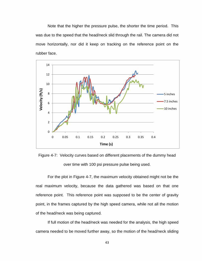
Note that the higher the pressure pulse, the shorter the time period. This
was due to the speed that the head/neck slid through the rail. The camera did not
move horizontally, nor did it keep on tracking on the reference point on the
rubber face.
Figure 4-7: Velocity curves based on different placements of the dummy head
over time with 100 psi pressure pulse being used.
For the plot in Figure 4-7, the maximum velocity obtained might not be the
real maximum velocity, because the data gathered was based on that one
reference point. This reference point was supposed to be the center of gravity
point, in the frames captured by the high speed camera, while not all the motion
of the head/neck was being captured.
If full motion of the head/neck was needed for the analysis, the high speed
camera needed to be moved further away, so the motion of the head/neck sliding
0
2
4
6
8
10
12
14
0 0.05 0.1 0.15 0.2 0.25 0.3 0.35 0.4
Ve
loci
ty (
ft/s
)
Time (s)
5 inches
7.5 inches
10 inches

44
through the rail could be taken with a new set of distance calibration. The
problem that the camera could not be moved any further as the tripod mounted to
the camera was already placed against the wall.
The plots in Figure 4.8 show the acceleration reaction over time with
different placements of the head/neck. The results shown are based on 50 psi
pressure pulses.
Figure 4-8: Moving average trend lines with 4 periods for acceleration curves
over time when 50 psi pressure pulse while the head is placed at 3 different
locations (reference point is 5, 7.5, 10 inches away from the shock tube opening).
In the plot above, there are two periods of time that have larger
magnitudes in acceleration, which are between 0 and 0.4 second and between
0.8 second and 1.2 second. They seem to have the same trends as the ones
-2
-1.5
-1
-0.5
0
0.5
1
1.5
2
0 0.2 0.4 0.6 0.8 1 1.2 1.4Acc
ele
rati
on
(g
)
Time (s)
4 per. Mov. Avg.
(5 inches)
4 per. Mov. Avg.
(7.5 inches)
4 per. Mov. Avg.
(10 inches)

45
between velocity and time. The closer the head/neck was to the shock tube
opening, the higher the maximum acceleration.
As the maximum acceleration should have occurred when the shock blast
hit the dummy head/neck, the acceleration at the beginning of the testing should
be taken into account for data analyzing, while the second half of the curves
could be neglected as the results there were supposed to be minimal. The plot in
Figure 4-9 is due to the unwanted vibrations and the second wave of blast hitting
the head.
The following plots (Figures 4-9 & 4-10) show the difference between
different placements of the head/neck after the second half of the curves got cut
off, while 75 psi and 100 psi pressure pulses were used for testing.
Figure 4-9: Acceleration curves based on different placements of the dummy
head with 75 psi pressure pulse being used.
-80
-60
-40
-20
0
20
40
60
0 0.05 0.1 0.15 0.2 0.25 0.3
Acc
ele
rati
on
(g
)
Time (s)
5 inches
7.5 inches
10 inches

46
Looked smoother and neater than in Figure 4-8, although the curves were
not based on the average of the three tests on each placement, the curves show
that the further the head/neck to the shock tube opening, the lower the maximum
acceleration.
Figure 4-10: Acceleration curves based on different placements of the dummy
head when 100 psi pressure pulse is used.
Figure 4-10 shows how the acceleration reacts under a 100 psi pressure
pulse. The curves are not as smooth as the ones before that, but the range for
the acceleration was increased as the setup pressure pulse was higher.
Using the tracking function from the high speed camera and the Motion
Studio software, the maximum velocity and acceleration could be determined.
As expected, the velocity started at zero and increased rapidly as the pressure
pulse hit the head/neck. Next it started slowing down from the medium and in
-80
-60
-40
-20
0
20
40
60
80
100
0 0.05 0.1 0.15 0.2 0.25 0.3
Acc
ele
rati
on
(g
)
Time (s)
5 inches
7.5 inches
10 inches

47
this case the air and the friction between the rails and the ball bearings bolted to
the sliding plate and the head stand. The maximum velocities for different
pressure pulses and distances are listed in Table 4-1.
5 inches 7.5 inches 10 inches
50 psi 2.839 ft/s 2.667 ft/s 2.397 ft/s
75 psi 6.504 ft/s 5.834 ft/s 5.535 ft/s
100 psi 12.744 ft/s 11.834 ft/s 10.890 ft/s
Table 4-1: Maximum velocities of the dummy head based on three tests on each
scenario.
It is shown here that the closer the head/neck to the shock tube opening,
the higher the maximum velocity. Although when the pressure pulse was set to
be higher, even the placement of the head/neck was placed further, and the
maximum velocity was still higher than the one with a lower pressure pulse and
shorter distance between the head/neck and the shock tube opening. Table 4-1
shows that the higher the pressure pulse was set for the testing, the greater the
difference on the maximum velocity between different placements of the
head/neck and the difference between the 5 and 10 inches cases.
Other than finding the maximum velocities of the dummy head, the
maximum accelerations on different cases could be found by using Excel. Table
4-2 shows the maximum accelerations obtained by using tracking.
48
5 inches 7.5 inches 10 inches
50 psi 3.296 g 2.668 g 2.529 g
75 psi 23.240 g 18.083 g 16.356 g
100 psi 72.820 g 58.852 g 42.324 g
Table 4-2: Maximum accelerations of the dummy head based on three tests on
each scenario.
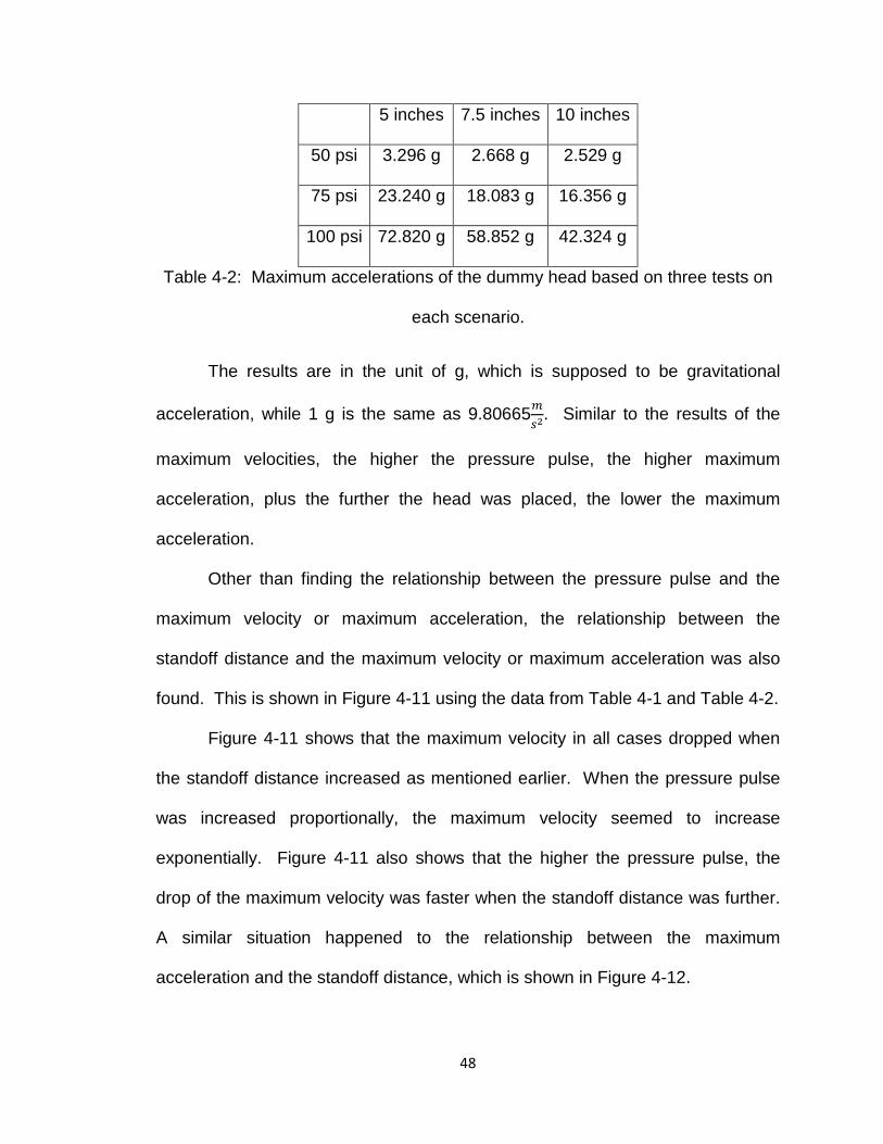
The results are in the unit of g, which is supposed to be gravitational
acceleration, while 1 g is the same as 9.80665$�. Similar to the results of the
maximum velocities, the higher the pressure pulse, the higher maximum
acceleration, plus the further the head was placed, the lower the maximum
acceleration.
Other than finding the relationship between the pressure pulse and the
maximum velocity or maximum acceleration, the relationship between the
standoff distance and the maximum velocity or maximum acceleration was also
found. This is shown in Figure 4-11 using the data from Table 4-1 and Table 4-2.
Figure 4-11 shows that the maximum velocity in all cases dropped when
the standoff distance increased as mentioned earlier. When the pressure pulse
was increased proportionally, the maximum velocity seemed to increase
exponentially. Figure 4-11 also shows that the higher the pressure pulse, the
drop of the maximum velocity was faster when the standoff distance was further.
A similar situation happened to the relationship between the maximum
acceleration and the standoff distance, which is shown in Figure 4-12.

49
Figure 4-11: Maximum velocity of the dummy head based on different standoff
distance (placement).
Figure 4-12: Maximum acceleration of the dummy head based on different
standoff distance.
0
2
4
6
8
10
12
14
4 5 6 7 8 9 10 11
Ma
xim
um
Ve
loci
ty (
ft/s
)
Standoff Distance (inches)
50 psi
75 psi
100 psi
0
10
20
30
40
50
60
70
80
4 5 6 7 8 9 10 11
Ma
xim
um
Acc
ele
rati
on
(g)
Standoff Distance (inches)
50 psi
75 psi
100 psi

50
4.2. Accelerometers Results
To get the results from using the accelerometers, an additional person
was needed for assistance. One person operated the butterfly valve and the
Motion Studio software on a computer while the other person communicated and
cooperated so he/she would be able to receive data from the accelerometers by
using LabVIEW on another computer. The following plot in Figure 4-13 is the
result obtained from one of 27 experiments performed.
Figure 4-13: Moving average trend lines with 200 periods for accelerations
curves with 50 psi pressure pulse is used when the reference point on the
dummy head is 5 inches away from the shock tube opening.
Figure 4-13 shows that when the blast hit the dummy head, there was a
jump in acceleration, in both x and y directions. The accelerations remained
-30
-20
-10
0
10
20
30
40
50
60
2 2.5 3 3.5
Acc
ele
rati
on
(g
)
Time (s)
200 per. Mov. Avg. (x)
200 per. Mov. Avg. (y1)
200 per. Mov. Avg. (y2)

51
constant for about 0.2 seconds then began to increase again. The curves finally
went back down to about 0 g within time duration of 1.5 seconds. The curves
also showed a lot of ups and downs (instability) especially after reaching the
maximum accelerations. That was due to the vibrations/movements of the
dummy head, or the friction between the bearings and the rails. The plot in
Figure 4-14 shows that the acceleration in the x-direction was usually higher than
the one in the y-direction, as the dummy head was hit in the x-direction. Note
that y1 is the acceleration curve representing an unfiltered result while y2 is the
filtered result for the acceleration in the y-direction.
Figure 4-14: Acceleration curves with 50 psi pressure pulse used while the
dummy head was set 10 inches away from the shock tube opening.
-30
-20
-10
0
10
20
30
40
50
60
1.5 1.7 1.9 2.1 2.3 2.5
Acc
ele
rati
on
(g
)
Time (s)
x
y1
y2

52
Figure 4-14 shows the acceleration curves a bit different than the one
shown earlier. Similar to the previous plot (Figure 4-13), the acceleration curves
on this plot also jumped at the beginning of the test and a constant acceleration
phase. Once again the curve started dropping down to about 0 g 0.6 seconds
after the release of the compressed air. As mentioned earlier, there was a total
of 27 performances conducted for this paper and after receiving all of the data by
using accelerometers and some modifications on the data, the maximum
accelerations in x-direction and y-direction were found, and they are all listed in
Table 4-3 and 4-4 with the results in the unit of g.
5 inches 7.5 inches 10 inches
50 psi 48.39 32.06 38.28
75 psi 50.89 25.72 19.07
100 psi 59.14 32.34 37.34
Table 4-3: Average maximum acceleration of the dummy head in x-direction.
5 inches 7.5 inches 10 inches
50 psi 58.46 21.67 30.44
75 psi 48.22 17.26 14.49
100 psi 145.88 48.69 21.42
Table 4-4: Average maximum acceleration of the dummy head in y-direction
(filtered).
The tables show a trend that when the placement of the dummy head was
set to be the same, the testing pressure pulse and the acceleration increased.
When the testing pressure pulse was set to be the same, the further the dummy

53
head was placed away from the shock tube opening and the lower the
acceleration. There were some exceptions in some cases, which were due to
some errors in the setup or the instability/accuracy of the devices.
After getting all the maximum values of maximum acceleration, they were
used to plot the maximum acceleration based on different standoff distances.
Figures 4-15 and 4-16 show the relationship between standoff distance and
maximum acceleration in both x-direction and y-direction by using
accelerometers.
Figure 4-15: Maximum acceleration of the dummy head based on standoff
distance in x-direction.
0
10
20
30
40
50
60
70
4 5 6 7 8 9 10 11
Acc
ele
rati
on
(g
)
Standoff Distance (inches)
50 psi
75 psi
100 psi
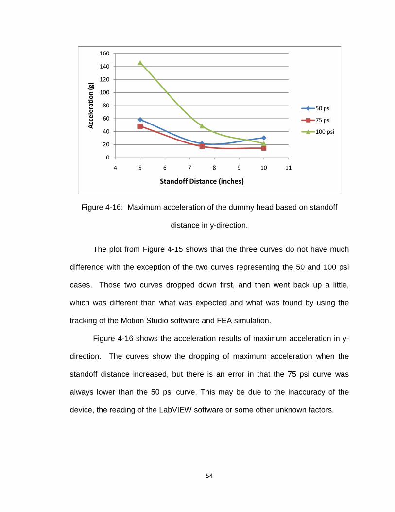
54
Figure 4-16: Maximum acceleration of the dummy head based on standoff
distance in y-direction.
The plot from Figure 4-15 shows that the three curves do not have much
difference with the exception of the two curves representing the 50 and 100 psi
cases. Those two curves dropped down first, and then went back up a little,
which was different than what was expected and what was found by using the
tracking of the Motion Studio software and FEA simulation.
Figure 4-16 shows the acceleration results of maximum acceleration in y-
direction. The curves show the dropping of maximum acceleration when the
standoff distance increased, but there is an error in that the 75 psi curve was
always lower than the 50 psi curve. This may be due to the inaccuracy of the
device, the reading of the LabVIEW software or some other unknown factors.
0
20
40
60
80
100
120
140
160
4 5 6 7 8 9 10 11
Acc
ele
rati
on
(g
)
Standoff Distance (inches)
50 psi
75 psi
100 psi

55
CHAPTER 5. FINITE ELEMENT ANALYSIS OF THE
SHOCK TUBE FLOW
This chapter is to describe the procedures for the FEA including the
descriptions, assumptions, and boundary conditions of the model that is being
used. Then results from this specific analysis are also shown.
5.1. LS-DYNA FE Software
LS-DYNA is used to simulate the motion/reaction of the Hybrid III dummy
head under shock wave of blast. LS-DYNA is mostly used for transient dynamic
FEA on more complex or real life problems, especially in the automobile and the
aerospace industries. This software helps in finding a wide variety of results
depending on what is wanted, such as the animation of the pressure, velocity
distributions of the result, pressure, velocity, acceleration, displacement, or
energy plots over a period of time on either a single node or a single element.
5.1.1. Preliminary Shock Tube Model
The model is made by using modeling software HyperMesh of the Atlair
Engineering Company. In HyperMesh, the geometries and meshing of the model
are done before being exported to LS-PrePost, where conditions would be done
at. Figure 5-1 shows what the model looks like.

56
Figure 5-1: Preliminary shock tube model in LS-DYNA.
The model has a total of four parts, which include the air inside the driver
section pipe, which has a color of light blue; the air with ambient condition, which
has a red color; the butterfly valve, which has a green color, and the head model
which is a yellow color. The center point of the head was set at 5, 7.5, and 10
inches away from the shock tube opening.
5.1.2. Condition Setups
There were a few conditions applied to the model. First of all, different
energies were applied to both air parts of the model, representing the 100 psi
and 14.7 psi pressures for the two air domains. A rigid body assumption was
then applied to the valve while the valve was constrained in all directions except
for the y-direction, so that the valve would turn along the y-axis, as shown as
Figure 5-2. The ‘Lagrange In Solid’ constrain was selected for the head model
as the head was in the air domain. Finally, all the outer surfaces were

57
constrained as it was assumed that they were in the inner surfaces of the shock
tube, meaning that there would be no placement, velocity, nor acceleration
changes.
Figure 5-2: a) Initial stage of the model, b) valve is turned 90 degrees.
5.1.3. Numerical Results on the Preliminary Model
After the simulation was complete, the results from the simulation could be
shown. Figure 5-3 shows the velocity curves for the results obtained by the
simulations.
Figure 5-3: Flow velocity with 100 psi pressure pulse.
-5
0
5
10
15
20
25
0 20 40 60 80 100 120
Ve
loci
ty (
ft/s
)
Time (ms)
5 inches
7.5 inches
10 inches

58
The plot in Figure 5-3 shows that when the head model was placed 5
inches away from the shock tube opening, the velocity of the head model began
to increase at roughly 20 ms after the release of the compressed air. The
maximum velocity of the head eventually increased to 19.2 ft/s. The other two
curves, representing the cases when the head model was placed 7.5 and 10
inches away from the shock tube opening, were relatively small compared to the
5 inch curve. Although the plot shows that when the head model was placed
closer to the shock tube opening, the higher the maximum velocity that it would
get.
Figure 5-4 is a plot showing the acceleration curves representing three
different areas on the surface of the head model when it was placed 5 inches
away from the shock tube opening and the three areas included the front, side,
and back of the head model.
Figure 5-4: Acceleration of the head model when it was placed 5 inches away
from the shock tube opening while 100 psi pressure pulse was used.
-800
-600
-400
-200
0
200
400
600
800
1000
0 20 40 60 80 100 120
Acc
ele
rati
on
(g
)
Time (ms)
Front
Side
Back

59
The plot shows that the frontal area of the head model had the highest
magnitude of acceleration (higher than the side and back of the head), while the
maximum acceleration on the frontal area topped at 818 g. The maximum values
are listed in Table 5-1.
Front Side Back
5 inches 818.08 g 137.71 g 180.56 g
7.5 inches 1.80 g 2.43 g 1.61 g
10 inches 5.78 g 1.44 g 0.89 g
Table 5-1: Maximum accelerations on different spots of the head model.
As shown, the values obtained from the 5 inches case were much larger
than those from the 7.5 and 10 inches cases. Such big differences could be due
to many factors, such as the energy loss due to the distance between the center
point of the head model and the shock tube opening, and the use of the valve
model while it took about 0.5 second to finish the 90 degree turn. To verify the
use of the valve, a research with experimental results by Varas et al was used.
5.1.4. Validation of existing model using FEM
In a research paper by Varas et al. published in 2011, a square tubing
shock tube (Figure 5-5) was used.
Figure 5-5: Shock Tube by J. M. Varas et al.
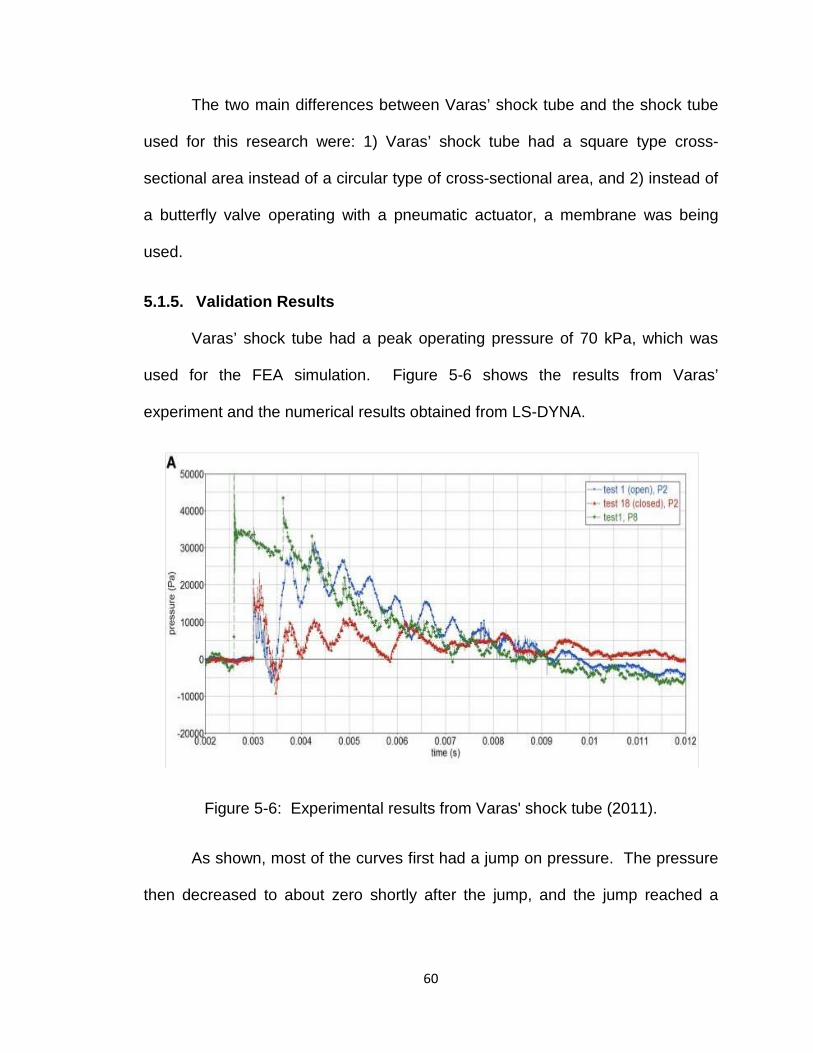
60
The two main differences between Varas’ shock tube and the shock tube
used for this research were: 1) Varas’ shock tube had a square type cross-
sectional area instead of a circular type of cross-sectional area, and 2) instead of
a butterfly valve operating with a pneumatic actuator, a membrane was being
used.
5.1.5. Validation Results
Varas’ shock tube had a peak operating pressure of 70 kPa, which was
used for the FEA simulation. Figure 5-6 shows the results from Varas’
experiment and the numerical results obtained from LS-DYNA.
Figure 5-6: Experimental results from Varas' shock tube (2011).
As shown, most of the curves first had a jump on pressure. The pressure
then decreased to about zero shortly after the jump, and the jump reached a

61
maximum pressure of about 34000 Pa. The plot in Figure 5-7 shows that the
positive phase of pressure had a duration time of about 7 ms.
Figure 5-7: Pressure plot based on different areas of the head model.
As shown in Figure 5-7, all of the pressure curves jumped up at about 20
ms, and had a positive phase duration of between 20 and 40 ms. For the curve of
frontal area of the head model, the pressure jumped up and topped at about 38
kPa. The pressure on the side area of the head model topped at about 32 kPa.
Both were very close to the experimental results obtained by Varas. The main
difference was the positive phase time duration. Such a difference would be due
to many factors, such as the accuracy of the FE model, the geometry of the
whole shock tube, and the model (synbone and gelatin were used for the
experimental work and steel was used for the FE model) of the ball.
-20
-10
0
10
20
30
40
50
0 20 40 60 80 100 120
Pre
ssu
re (
kP
a)
Time (ms)
Front
Side
Back

62
5.1.6. Modified Model for the Blast Shock Tube
The new model was similar to the previous one used, but the valve was
removed. The previous model involved the placement change (5, 7.5, and 10
inches) with one pressure (100 psi), and the new model involved one placement
(5 inches) with different pressure pulse sets (50, 75, and 100 psi). Figure 5-8
shows the meshed model with only three separate parts for the simulation.
Figure 5-8: Modified shock tube model for simulation.
5.1.7. Results on the New Model
After some changes on boundary conditions, the problem could be solved.
Figure 5-9 is the velocity plot for this new shock tube model.

63
Figure 5-9: Velocity distribution of the head model based on different pressure
pulses (50, 75, and 100 psi) when the middle point of the head was 5 inches
away from the shock tube opening.
As expected, the 100 psi curve had the highest values among all three
cases, then 75 psi had the next highest, and finally the 50 psi curve had the
lowest values. This indicates that the higher the pressure pulse, the greater the
movement of the head model, or any test object used for the blast. The maximum
velocities are listed in Table 5-2.
Maximum Velocity
50 psi 18.92 ft/s
75 psi 26.51 ft/s
100 psi 32.74 ft/s
Table 5-2: Maximum velocities from the modified shock tube model and head.
-5
0
5
10
15
20
25
30
35
0 20 40 60 80
Ve
loci
ty (
ft/s
)
Time (ms)
50 psi
75 psi
100 psi

64
Other than the velocity plot, the acceleration plot could also be found by
using the software, and Figure 5-10 is an acceleration plot for a specific case.
Figure 5-10: Acceleration plot with 50 psi pressure pulse with 5 inches head
placement.
The results were similar to the results from when the valve was involved
as the frontal area of the head model had the highest magnitude of acceleration
rather than the side and back of the head model. The maximum accelerations
for the three different cases are listed in Table 5-3.
Front Side Back
50 psi 525.59 g 86.16 g 114.53 g
75 psi 1181.13 g 115.11 g 196.43 g
100 psi 2541.28 g 137.78 g 234.37 g
Table 5-3: Maximum velocities due to different pressure pulses on various spots
of the head model.
-700
-500
-300
-100
100
300
500
0 20 40 60 80 100
Acc
ele
rati
on
(g
)
Time (ms)
Front
Side
Back

65
The acceleration on the frontal area of the head model had a significant
increase from the case of 50 psi to the case of 100 psi, which had a difference of
about 2000 g. The differences on the side and back of the head model were
relatively small compared to the result for the frontal area case, meaning that the
acceleration on the frontal area of the head was affected the most when the
pressure pulse was changed. Such affect is plotted in Figure 5-11.
Figure 5-11: Acceleration based on pressure pulses on different spots of the
head.
Other than the velocity and acceleration plots, pressure plots were also
made. Pressure distribution on the head played a big role in this research. The
plot in Figure 5-12 shows the pressure responses on different spots of the head
model and the plot in Figure 5-13 shows the pressure difference on the front area
of the head model with different pressure pulses.
0
500
1000
1500
2000
2500
3000
40 60 80 100
Acc
lera
tio
n (
g)
Pressure Pulse (psi)
Front
Side
Back

66
Figure 5-12: Pressure plot with 50 psi pressure pulse on different places of the
head model.
Figure 5-13: Pressure on front area of the head with different pressure pulses.
Similar to the acceleration results, the acceleration on the frontal area of
the head model had the greatest values among the three areas, but the pressure
-5
0
5
10
15
20
25
30
0 20 40 60 80 100
Pre
ssu
re (
ksi
)
Time (ms)
Front
Side
Back
-20
-10
0
10
20
30
40
50
60
70
0 20 40 60 80 100 120
Pre
ssu
re (
ksi
)
Time (ms)
50 psi
75 psi
100 psi
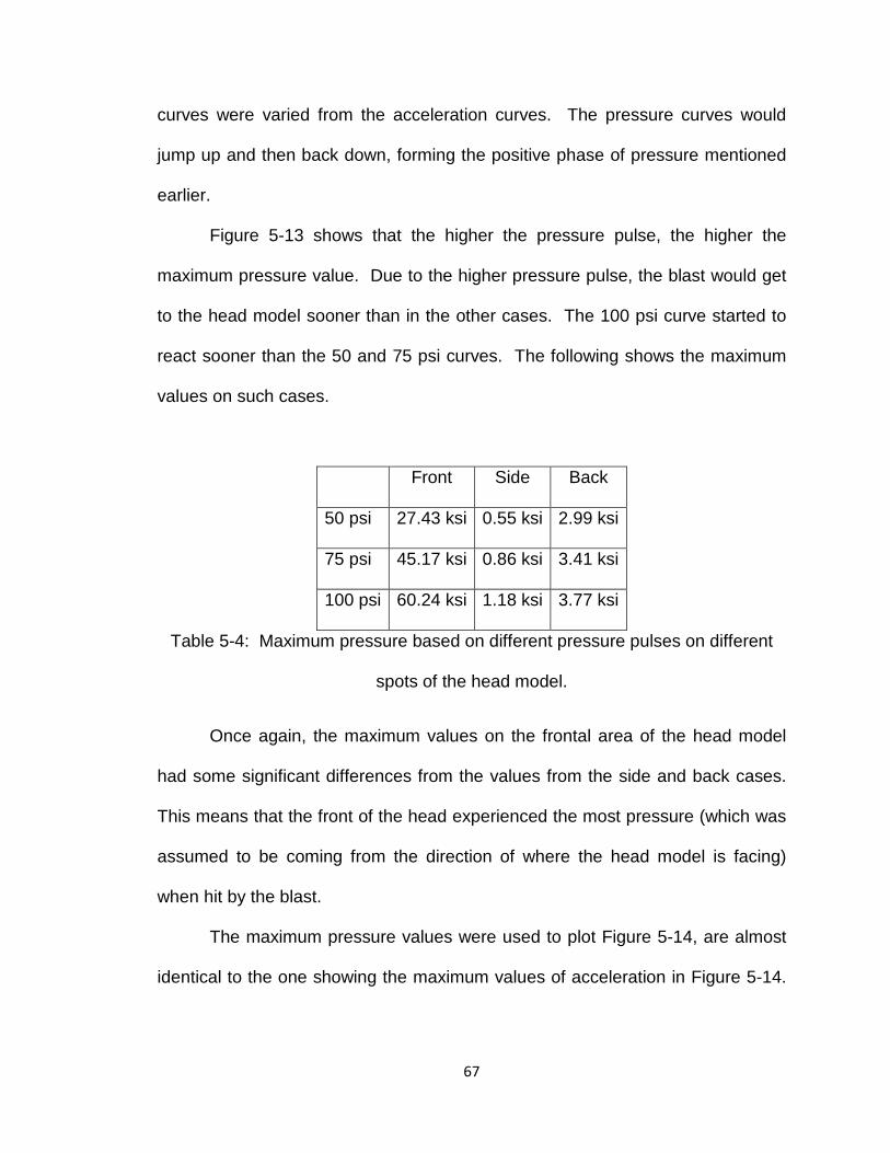
67
curves were varied from the acceleration curves. The pressure curves would
jump up and then back down, forming the positive phase of pressure mentioned
earlier.
Figure 5-13 shows that the higher the pressure pulse, the higher the
maximum pressure value. Due to the higher pressure pulse, the blast would get
to the head model sooner than in the other cases. The 100 psi curve started to
react sooner than the 50 and 75 psi curves. The following shows the maximum
values on such cases.
Front Side Back
50 psi 27.43 ksi 0.55 ksi 2.99 ksi
75 psi 45.17 ksi 0.86 ksi 3.41 ksi
100 psi 60.24 ksi 1.18 ksi 3.77 ksi
Table 5-4: Maximum pressure based on different pressure pulses on different
spots of the head model.
Once again, the maximum values on the frontal area of the head model
had some significant differences from the values from the side and back cases.
This means that the front of the head experienced the most pressure (which was
assumed to be coming from the direction of where the head model is facing)
when hit by the blast.
The maximum pressure values were used to plot Figure 5-14, are almost
identical to the one showing the maximum values of acceleration in Figure 5-14.

68
This means that the front surface of the head was affected the most by the
change of the pressure pulse.
Figure 5-14: Maximum pressure on different spots of the dummy head based on
different pressure pulses being used.
5.2. Computational Fluid Dynamics (ANSYS – CFX)
To understand the air flow’s reaction over a period of time after the blast
was initiated, ANSYS-CFX was used. ANSYS-CFX is a high-performance
software that helps solve fluid dynamic problems.
5.2.1. Air Flow Model
The air flow model was first created by using the classic ANSYS program,
due to the familiarity of the software and the model was then imported into
ANSYS-CFX. Once ANSYS-CFX was used, all the meshing, conditions applying,
0
10
20
30
40
50
60
70
40 50 60 70 80 90 100 110
Pre
ssu
re (
ksi
)
Pressure Pulse (psi)
Front
Side
Back
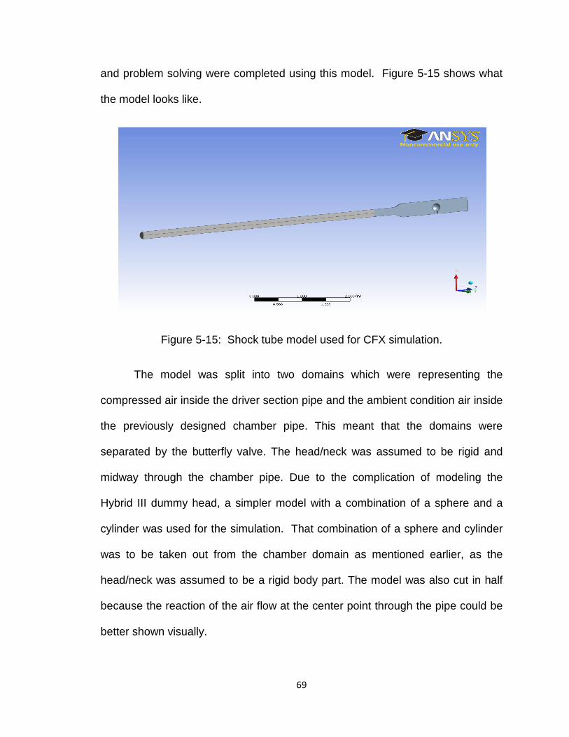
69
and problem solving were completed using this model. Figure 5-15 shows what
the model looks like.
Figure 5-15: Shock tube model used for CFX simulation.
The model was split into two domains which were representing the
compressed air inside the driver section pipe and the ambient condition air inside
the previously designed chamber pipe. This meant that the domains were
separated by the butterfly valve. The head/neck was assumed to be rigid and
midway through the chamber pipe. Due to the complication of modeling the
Hybrid III dummy head, a simpler model with a combination of a sphere and a
cylinder was used for the simulation. That combination of a sphere and cylinder
was to be taken out from the chamber domain as mentioned earlier, as the
head/neck was assumed to be a rigid body part. The model was also cut in half
because the reaction of the air flow at the center point through the pipe could be
better shown visually.
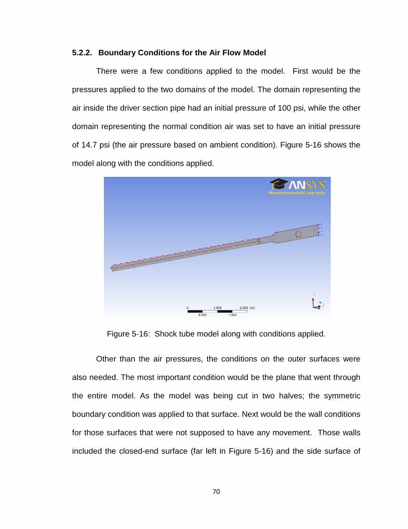
70
5.2.2. Boundary Conditions for the Air Flow Model
There were a few conditions applied to the model. First would be the
pressures applied to the two domains of the model. The domain representing the
air inside the driver section pipe had an initial pressure of 100 psi, while the other
domain representing the normal condition air was set to have an initial pressure
of 14.7 psi (the air pressure based on ambient condition). Figure 5-16 shows the
model along with the conditions applied.
Figure 5-16: Shock tube model along with conditions applied.
Other than the air pressures, the conditions on the outer surfaces were
also needed. The most important condition would be the plane that went through
the entire model. As the model was being cut in two halves; the symmetric
boundary condition was applied to that surface. Next would be the wall conditions
for those surfaces that were not supposed to have any movement. Those walls
included the closed-end surface (far left in Figure 5-16) and the side surface of
71
the driver section pipe, the side surface of the chamber pipe, and the surfaces
involving the head/neck geometry.
The other end of the chamber air, the side away from the closed-end of
the driver section air had an opening boundary condition (far right in Figure 5-16),
as that would allow the pressure blast to leave when it got to the end of the air
domain instead of bouncing back inside the chamber. As the wall was supposed
to be a steel surface, a sand grain roughness of 0.0018 inches was assumed into
the simulation setup. Other than that, the interface between the two domains was
set to have the default condition. The termination time was to be 20 ms. Finally,
the last condition that needed to be applied was the initial condition. In this case,
the two air domains were to be set to have initial velocities of zeroes in all three
directions because before the air started to move through the shock tube, the air
inside the driver section pipe and the chamber pipe were supposed to be stable.
5.2.3. Pressure Distribution inside the Shock Tube
After all the geometry modeling, meshing and conditions applying were
complete, the simulation could begin. The transient type simulation usually took a
lot longer than running a regular static analysis simulation. That may have been
due to the calculation on every single element of the model over a period of time
with a specific time step. The plots in Figure 5-17 show the pressure distribution
of the air inside the chamber pipe.
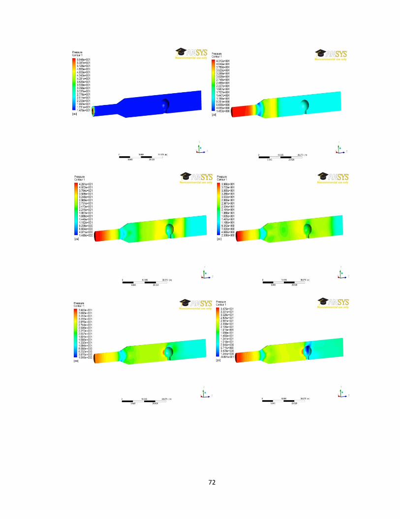
72
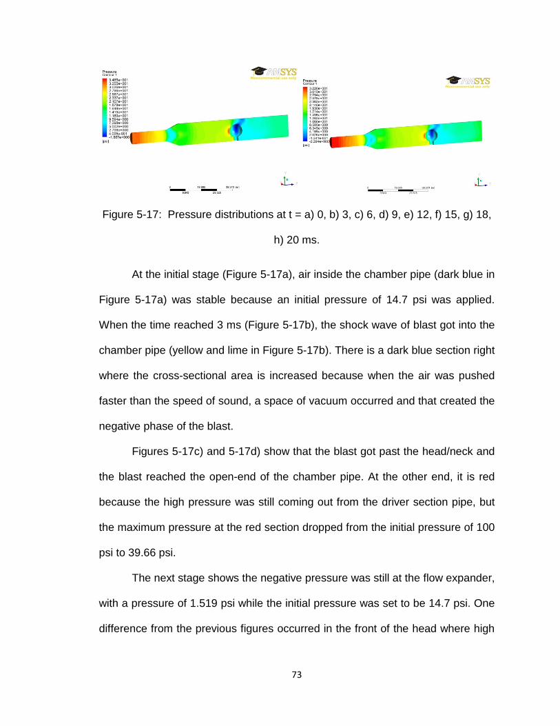
73
Figure 5-17: Pressure distributions at t = a) 0, b) 3, c) 6, d) 9, e) 12, f) 15, g) 18,
h) 20 ms.
At the initial stage (Figure 5-17a), air inside the chamber pipe (dark blue in
Figure 5-17a) was stable because an initial pressure of 14.7 psi was applied.
When the time reached 3 ms (Figure 5-17b), the shock wave of blast got into the
chamber pipe (yellow and lime in Figure 5-17b). There is a dark blue section right
where the cross-sectional area is increased because when the air was pushed
faster than the speed of sound, a space of vacuum occurred and that created the
negative phase of the blast.
Figures 5-17c) and 5-17d) show that the blast got past the head/neck and
the blast reached the open-end of the chamber pipe. At the other end, it is red
because the high pressure was still coming out from the driver section pipe, but
the maximum pressure at the red section dropped from the initial pressure of 100
psi to 39.66 psi.
The next stage shows the negative pressure was still at the flow expander,
with a pressure of 1.519 psi while the initial pressure was set to be 14.7 psi. One
difference from the previous figures occurred in the front of the head where high

74
pressure was created with a pressure of 39.22 psi, as the high speed flow was
being slowed down by the head.
The next three plots (Figures 5-17 e f g) are extremely similar in that the
maximum pressure occurred where the compressed air was being released or in
front of the head. The minimum pressure section was moved from the flow
expander to somewhere behind the head, and it was getting lower over time. In
Figure 5-17e, the minimum pressure dropped to -0.989 psi, and in Figure 5-17g,
it kept going down to -2.294 psi. Other than the pressure distribution animation,
pressure or velocity at any point in the system can also be shown. The following
plots (Figure 5-18) show the velocity and pressure curves at a few specific points
in the system so different reactions can be seen.
Figure 5-18: Pressure vs. Time plot at 5 different spots in the system.
The first point selected for the plot was one foot away from the butterfly
valve at the center point of the circular flow. As shown, the pressure increased to
0
5
10
15
20
25
30
35
40
45
50
0 0.005 0.01 0.015 0.02
Pre
ssu
re (
psi
)
Time (s)
1 ft
2.5 fts
Front of head
Behind head
Oblique Shock
75
roughly 47 psi from 14.7 psi in 1.1 ms, due to the rapid air flow going through the
point. Then the pressure decreased slowly as the compressed air coming out
from the driver section pipe was getting less pressure, it decreased to 29.43 psi
at t=20ms, but, in time, will likely return to ambient pressure.
The second point selected was 2.5 feet away from the butterfly valve. The
curve shows that there was a pressure jump at about t=2.5 ms. The pressure
then dropped below 14.7 psi, meaning that the negative pressure was created
due to the high speed of air flow.
The other three points selected were at the front of the head, behind the
head, and at the end of the flow expander. In the case of in front of the head, the
pressure simply increased when the blast reached the front of the head. The
pressure then decreased some but increased again as the second wave of blast
approached.
Figure 5-19 shows the velocity plot at different points in the system over a
time period of 20 ms, which is the same as the ones selected for the previous
plot. The first one was one foot away from the butterfly valve and the curve
shows a jump of velocity at about 1 ms and then it went up slowly. The curve
went up slowly because the point was so close to the valve, keeping the air flow
stable enough to have such distribution. The point that was 2.5 feet away from
the valve had a velocity distribution that is shown as the red curve. It first went up
due to the blast, and then the curve continued to go up rapidly until it got to about
1200 ft/s and then the velocity remained at that range 5 ms after the blast began.
The second increase of velocity on the second point was supposed to be due to

76
the Prandtl-Meyer expansion fan process, meaning that when the air flow was
having a speed over the speed of sound and reaching to an increase of the
cross-sectional area of the testing pipe, the velocity of the air flow would
increase.
Figure 5-19: Velocity vs. time plot at five different spots in the system.
The velocity curves for the other three points were relatively small
compared to the other two points mentioned earlier. This was due to the flow
hitting on the head and the flow being limited by the oblique shock. The air flow
in the chamber pipe had a maximum velocity of roughly 1900 ft/s (about Mach
1.7) at where the cross-sectional area started getting larger. This was also due to
the Prandtl-Meyer expansion fan process.
-200
0
200
400
600
800
1000
1200
1400
1600
0 0.005 0.01 0.015 0.02
Ve
loci
ty (
ft/s
)
Time (s)
1 ft
2.5 ft
Front of Head
Behind Head
Oblique Shock

77
CHAPTER 6. CONCLUSIONS
In this thesis, experimental and numerical approaches were used to
determine the linear velocity, acceleration, and pressure of the Hybrid III dummy
head when it is hit by shock waves from a blast. For the experimental approach,
a blast shock tube was built for the laboratory settings. For the numerical
approach, a simple elastic FE head/neck model was used for the dynamic
simulation. The relationships between the pressure pulse and the linear
acceleration/velocity and the standoff distance were found.
The following are some conclusions made based on the results obtained
from the experiments:
1. When the operating pressure pulse is increased proportionally, the
maximum velocity and acceleration of the head/neck increase
exponentially when sliding through the rails.
2. As the operating pressure pulse is set to be higher, the instability on the
velocity curves increases. When 50 psi pressure pulse is used, the
velocity curve is more linear than the ones for the 50 and100 psi pressure
pulses; and that would be due to the bending movement of the head/neck,
rippling of the rubber face, and the friction caused by the rails.
3. When the dummy head is placed at a specific standoff distance, it shows
that when the operating pressure pulse gets higher, the difference
between the maximum velocity values gets larger.
78
4. Similar to the results for the maximum velocities, it shows that when the
operating pressure pulse gets higher, the difference between the
maximum acceleration values also gets larger.
5. From the results obtained by using accelerometers, it is shown that the
accelerations would go down when lowering the setup pressure pulse, or
when placing the dummy head further away from the shock tube opening,
but with some unexpected results at the same time. The unexpected
results could be due to the inaccuracy of accelerometers setup, the
inaccuracy of the accelerometers readings, the instability of the air flow,
noise, or the vibrations of the dummy head caused by the blast.
In another part of the research, a simple elastic model was used for FEA
focusing on the air flow and the dummy head. This is mainly based on the
reactions of the head/neck model.
1. When the FE model has a valve involved, it shows that when the
head/neck model is placed 5 inches away from the shock tube opening,
the velocity of the head/neck is much higher than the ones when the head
model is placed 7.5 and 10 inches away from the shock tube opening.
That would be due to the instability of the flow caused by the turning valve.
2. As the model including the valve had some unexpected results, a few
more simulations were done with the same model, but with the valve part
removed. In this case, the results are showed two facts: 1) when the head
is set to be at the same placement for all the simulations, the higher the
pressure pulse is set, the higher the velocity, acceleration, and pressure is

79
on the head model, and 2) the frontal area of the head model is always
having the highest pressure among the three different spots of the head
model including the frontal, side, and back surfaces of the head model.
The last part of the research is also involved the FEA, but it is
concentrated on the air flow inside the pre-designed testing chamber instead of
on the velocity and acceleration of the Hybrid III dummy head.
The following are some conclusions made based on the results obtained from the
analyses:
1. Two different pressures were applied to the two air domains in the model.
One had a pressure of 100 psi while the other has a pressure of 14.7 psi.
Although there was only an interface separating the two domains, the
maximum pressure of the air inside the chamber pipe increased instantly
to roughly 56.5 psi.
2. Within the 20 ms time period of simulation, the value of maximum
pressure dropped slowly, and the place of the maximum pressure kept
changing between the butterfly valve and the front of the head.
3. The maximum velocity of the air flow occurred at the flow expander, as the
direction of the air flow became more unidirectional before the air went to
the flow expander section. The air flow in the same section had a higher
velocity than the other sections of the chamber pipe as well. This was due
to the Prandtl-Meyer expansion fan process. Assuming the speed of
sound is 1126 ft/s, the maximum velocity of the flow there was found to be
80
roughly 1622 ft/s, which turned out to have a Mach number of 1.44,
meaning that the air flow reached the level of supersonic.
4. Negative pressure (lower than 14.7 psi) happened at two spots when the
compressed air flowed through the chamber. One was at the beginning of
the flow expander and the other was at the backside of the head. The
negative pressure happened because of the high speed of the air flow but
it does not last for long.

81
CHAPTER 7. RECOMMENDATIONS FOR FUTURE
STUDIES
The following are some recommendations for the research in the future:
1. The chamber pipe was extremely heavy and it would be more convenient
if it had been lighter. The unused chamber pipe, along with the flow
expander weighed a few hundred pounds, and it was, therefore, very
difficult to move; it was also connected to a stand had to be moved up and
down. It would be possible to find a six feet long acrylic chamber pipe with
a thickness of half an inch. Once the transparent chamber pipe was used
for the experimental setup, the reaction of the Hybrid III dummy head
could be captured by a high speed camera which would be easier and
safer.
2. There was an extremely small leakage of pressure coming out from the
butterfly valve. Results would be more accurate if the leakage problem
was repaired. The shock tube designed for this research used a
pneumatic actuator along with a solenoid and a butterfly valve. The minor
loss of pressure from the butterfly valve may have affected the
experimental results and the results could perhaps be improved if the
butterfly valve was replaced by using a diaphragm.
3. More components such as more pressure sensors or flow velocity
transducers at different spots inside the chamber pipe could be added to
82
the laboratory settings. This would help with understanding the pressure
and velocity distributions of the air flow for the specific shock tube.
4. There may have been more errors due to the size and turning time (it took
about 0.5 seconds when no compressed air was inside the driver section
pipe) of the butterfly valve, as it may have caused a significant loss of
pressure. The design of the shock tube may need to be changed to use a
membrane instead of the butterfly valve.
5. For the FEA part of the research, a more accurate model is needed. The
FE model of the Hybrid III dummy head includes the rubber and metal part
of the head and neck, meaning that the head/neck model would have
different mechanical properties. Having a ballistic helmet model would
help in understanding the usage/effect of a ballistic helmet and could be
beneficial in understanding the entire blast model.
83
REFERENCES CITED
Anderson, R.J. (2008). Shell Shock: An Old Injury with New Weapons. Molecular Interventions, 8, 204-218.
Boyer, D.W. (1960). An experimental study of the explosion generated by a pressurized sphere. Journal of Fluid Mechanics, 9. 401-29. Brooks, A. J., Clasper, J., Midwinter, M. J., Hodgetts, T. J., & Mahoney, P. F., Ryan’s Ballistic Trauma: A Practical Guide, New York: Springer, 1997. Print. CFX. (2012). Computer Software. Canonsburg, PA: ANSYS. Chafi, M.S., Dirisala, V., Karami, G., & Ziejewski, M. (2010). A FE parametric study of the dynamic response of the human brain with different CSF constitutive properties. Bio-Medical Materials and Engineering. DOI 10.3233/BME-2010-0619. Chafi, M.S., Karami, G., & Ziejewski, M., (2010). Biomechanical Assessment of Brain Dynamic Responses Due to Blast Pressure Waves. Annals of Biomedical Engineering, 38. 490-504. Chafi, M.S., Karami, G., & Ziejewski, M. (2009). Numerical analysis of blast-induced wave propagation using FSI and ALE multi-material formulations. International Journal of Impact Engineering, 36. 1269-1275. Helmick et al. (2006). Defense and Veterans Brain Injury Center Working Group on the Acute Management of Mild Traumatic Brain Injury (mTBI) in Military Operational Settings. Clicical Practice Guideline and Recommendations. Washington, DC: Defense and Veterans Brain Injury Center. Cifu et al. (2009). Defense and Veterans Brain Injury Center Consensus Conference. Acute Management of Concussion/mild Traumatic Brain Injury (mTBI) in the Deployed Setting. Washington, DC: Defense and Veterans Brain Injury Center. Dirisala, V., Karami, G., & Ziejewski, M. (2011). Effects of neck damping properties on brain response underimpact loading. International Journal for Numerical Methods in Biomedical Engineering. DOI: 10.1002/cnm. 1480.
Dobratz, B.M., & Crawford, P.C. (1985). LLNL Explosives Handbook, Properties of Chemical Explosives and Explosives Stimulants; UCRL-52997; Lawrence Livermore Laboratory: Livermore CA.

84
Finkelstein, E., Corso, P., & Miller, T. (2006). The Incidence and Economic Burden of Injuries in the United States. New York (NY): Oxford University Press. Gibson, P. (1994). Blast overpressure and survivability calculations for various sizes of explosive charges. Technical Report. Army Natick Research Development and Engineering Center MA.
Glasser, R.J. (2007, April). A Shock Wave of Brain Injuries. Retrieved from http://dva.state.wi.us/Docs/TBI/A_ShockWave_of_Brain_Injuries.pdf
HyperMesh Computer Software. Troy, MI: Altair Engineering. (2012).
Karami, G., Grundman, N., Abolfathi, N., Naik, A., & Ziejewski, M. (2009). A micromechanical hyperelastic modeling of brain white matter under large deformation. Journal of the Mechanical Behavior of Biomedical Materials, 2. 243-254. Kinney, G.F., Graham, K.K. (1985). Explosive Shocks in Air. Springer-Verlag New York Inc., New York.
LabView (Version 8.6) Computer Softwar]. Austin, TX: National Instruments. (2012).
Leonardi, A. D. C., Bir, C. A., Ritzel, D. V., & VandeVord, P. J. (2011, January). Intracranial Pressure Increases during Exposure to a Shock Wave. Journal of Neurotrauma, 28, 85-94.
LS-DYNA (Version 971) Computer Software. Livermore, CA: Livermore Software Technology Corporation. (2012). Magnuson, S. (2010). Scientists Hope Bomb Blast Research Can Lead to Better Helmets. National Defense, 95. Management of Concussion/mTBI Working Group. (2009). VA/DoD Clinical Practice Guideline for Management of Concussion/mild Traumatic Brain Injury: VA/DoD Evidence Based Practice. Washington, DC: Department of Veterans Affairs. Nahum, A.M., Smith, R., & Ward, C.C. (1977). Intracranial pressure dynamics during head impact. Proceedings of the 21st Stapp Car Crash Conference, 339-366。

85
Segars. R. A., & Carboni, M. G. (2008). A Shock Tube for Downselecting Material Concepts for Blast Protection Part I: Description of the Shock Tube and a Comparison of Flush Mounted and Recess Mounted Pressure Sensors. U.S. Army Natick Soldier Research, Development and Engineering Center. Sharma, S., & Zhang, L. (2011). Prediction Of Intracranial Responses from Blast Induced Neurotrauma using a Validated Finite Element Model of Human Head. Tan, P., Lee, B., & Tsangalis, C. (2010). Finite element analysis of sandwich panels subjected to shock tube blast loadings. Journal of Sandwich Structures and Materials OnlineFirst, 1-16. Tanielian, T., Jaycox, L. H. (EDS.) (2008). Invisible Wounds of War: Psychological and Cognitive Injuries, their Consequences, and Services to Assist Recovery. Santa Monica, CA: RAND Center for Military Health Policy Research. Varas, J. M., Philippens, M., Meijer, S. R., van den Berg, A. C., Sibma, P. C., van Bree, J. L. M. J., & de Vries, D. V. W. M. (2012). Physics of IED Blast Shock Tube Simulations for mTBI Research. Frontiers in Neurology. V.2. WebRef1: Brain Injuries and Mass Casualty Events. (2005). Retrieved from http://emergency.cdc.gov/masscasualties/braininjuriespro.asp WebRef2: Explosions and Blast Injuries: A Primer for Clinicians. (2012). Retrieved from http://emergency.cdc.gov/masscasualties/braininjuriespro.asp
WebRef3: Explosives. (2011). Retrieved from http://www.globalsecurity.org/military/systems/munitions/explosives.htm WebRef4: Traumatic Brain Injury. (2012). Retrieved from www.ninds.nih.gov/disorders/tbi/tbi.htm Ziejewski, M., Karami, G., & Akhatov, I. (2007). Selected Biomechanical Issues of Brain Injury Caused by Blasts. Brain Injury/professional, vol. 4 issue 1.