session 7 bivariate data and analysis - learner · pdf filesession 7 bivariate data and...

Data Analysis, Statistics, and Probability - 189 - Session 7

Session 7

Bivariate Data and Analysis

Key Terms for This Session

Previously Introduced• mean • standard deviation

New in This Session• association • bivariate analysis • contingency table

• co-variation • least squares line • line of best fit

• quadrants • scatter plot • sum of squared errors

IntroductionIn previous sessions, you provided answers to statistical problems by collecting and analyzing data on one vari-able. This kind of data analysis is known as univariate analysis. It is designed to draw out potential patterns in thevariation in order to provide better answers to statistical questions. In your exploration of univariate analysis, youinvestigated several approaches to organizing data in graphs and tables, and you explored various numericalsummary measures for describing characteristics of a distribution.

In this session, you will study statistical problems by collecting and analyzing data on two variables. This kind ofdata analysis, known as bivariate analysis, explores the concept of association between two variables. Associationis based on how two variables simultaneously change together—the notion of co-variation.

Learning ObjectivesThe goal of this lesson is to understand the concepts of association and co-variation between two quantitativevariables. In your investigation, you will do the following:

• Graph bivariate data in a scatter plot

• Divide the points in a scatter plot into four quadrants

• Summarize bivariate data in a contingency table

• Model linear relationships

• Explore the least squares line

Session 7 - 190 - Data Analysis, Statistics, and Probability

A Bivariate Data QuestionHave you ever wondered whether tall people have longer arms than short people? We’ll explore this question bycollecting data on two variables—height and arm length (measured from left fingertip to right fingertip).

Ask a question:

One way to ask this question is, “Is there a positive association between height and arm span?”

Through this question, we are seeking to establish an association between height and arm span. A positiveassociation between two variables exists when an increase in one variable generally produces an increase inthe other. For example, the association between a student’s grades and the number of hours per week thatstudent spends studying is generally a positive association. A negative association, in contrast, exists when anincrease in one variable generally produces a decrease in the other. For example, the association between thenumber of doctors in a country and the percentage of the population that dies before adulthood is generallya negative one.

There are many other ways to ask this same question about height and arm span. Here are two, which we willconcentrate on in Part A:

• Do people with above-average arm spans tend to have above-average heights?

• Do people with below-average arm spans tend to have below-average heights?

Collect appropriate data:

In Session 1, measurements (in centimeters) were given for the heights and arm spans of 24 people. Here arethe collected data, sorted by increasing order by arm span:

This is bivariate data, since two measurements are given for each person.

Problem A1. The data given above are sorted by arm span. Are they also sorted by height? If not exactly, are theygenerally sorted by height, and, if so, in which direction? Does this suggest any type of association betweenheight and arm span?

Part A: Scatter Plots (45 minutes)

Person # Arm Span Height Person # Arm Span Height

1 156 162 13 177 173

2 157 160 14 177 176

3 159 162 15 178 178

4 160 155 16 184 180

5 161 160 17 188 188

6 161 162 18 188 187

7 162 170 19 188 182

8 165 166 20 188 181

9 170 170 22 188 192

10 170 167 23 194 193

11 173 185 23 196 184

12 173 176 24 200 186


Problem A2.

a. Measure the arm span (fingertip to fingertip) and height (without shoes) to the nearest centimeter for sixpeople, including yourself.

b. Does the information you collected generally support or reject the observation you made in Problem A1?

c. Identify the person in the table whose arm span and height are closest to your own arm span and height.

Building a Scatter PlotAnalyze the data:

We will now begin our analysis of the bivariate data and explore the co-variation in the arm span and heightdata. Here again are the collected arm spans and heights for 24 people, sorted in increasing order by arm span:

Bivariate data analysis employs a special “X-Y”coordinate plot of the data that allows you to visualize the simul-taneous changes taking place in two variables. This type of plot is called a scatter plot. [See Note 1]

For our data, we will assign the X and Y variables as follows:

X = Arm Span

Y = Height

To see how this works, let’s examine the 10th person in the data table. Here are the measurements for Person 10:

X = Arm Span = 170 and Y = Height = 167

Part A, cont’d.

Note 1. The scatter plot, an essential component in this session, provides a graphical representation for bivariate data and for studying therelationship between two variables. Throughout this session, you will consider the connection between the graphical representations of con-cepts and numerical summary measures.

Remember that each person in the data is represented by the coordinate pair (X, Y), or one point in the scatter plot.


1 156 162 13 177 173

2 157 160 14 177 176

3 159 162 15 178 178

4 160 155 16 184 180

5 161 160 17 188 188

6 161 162 18 188 187

7 162 170 19 188 182

8 165 166 20 188 181

9 170 170 22 188 192

10 170 167 23 194 193

11 173 185 23 196 184

12 173 176 24 200 186


Person 10 is represented by the coordinate pair (170, 167) and is represented in the scatter plot as this point:

Let’s add two more points to the scatter plot, corresponding to Persons 2 and 23:

Problem A3. Judging from the scatter plot, does there appear to be a positive association between arm span andheight? That is, does an increase in arm span generally lead to an increase in height?

Part A, cont’d.

Here is the completed scatter plot for all 24 people:

Person # Arm Span Height

2 157 160

23 196 184


The scatter plot illustrates the general nature of the association between arm span and height. Reading from leftto right on the horizontal scale, you can observe that narrow arm spans tend to be associated with people whoare shorter, and wider arm spans tend to be associated with people who are taller—that is, there appears to be anoverall positive association between arm span and height.

A Further QuestionNow that we have established that there is a positive association between arm span and height, a new questionemerges: How strong is the association between arm span and height? Here again is the data for the 24 people:

In order to answer this question, let’s note the mean arm span and height for these 24 adults:

Mean arm span = 175.5 cm

Mean height = 174.8 cm

Problem A4.

a. Is your arm span and height above the average of these 24 adults?

b. How many of the 24 people have above-average arm spans?

c. How many of the 24 people have above-average heights?

d. It is possible to divide the 24 people into four categories: above-average arm span and above-averageheight; above-average arm span and below-average height; below-average arm span and above-averageheight; and below-average arm span and below-average height. How many of the 24 people fall into eachof these categories?

Part A, cont’d.

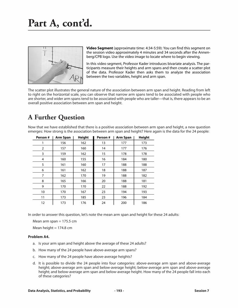
Video Segment (approximate time: 4:34-5:59): You can find this segment onthe session video approximately 4 minutes and 34 seconds after the Annen-berg/CPB logo. Use the video image to locate where to begin viewing.

In this video segment, Professor Kader introduces bivariate analysis. The par-ticipants measure their heights and arm spans and then create a scatter plotof the data. Professor Kader then asks them to analyze the associationbetween the two variables, height and arm span.


1 156 162 13 177 173

2 157 160 14 177 176

3 159 162 15 178 178

4 160 155 16 184 180

5 161 160 17 188 188

6 161 162 18 188 187

7 162 170 19 188 182

8 165 166 20 188 181

9 170 170 22 188 192

10 170 167 23 194 193

11 173 185 23 196 184

12 173 176 24 200 186


Problem A5.

a. Where would your arm span and height appear on thescatter plot?

b. Can you identify a person with an above-average armspan and height?

c. Can you identify a person with a below-average arm spanand an above-average height?

d. Can you identify a person with a below-average arm spanand height?

e. Can you identify a person with an above-average armspan and a below-average height?

Problem A6. Adding a vertical line to the scatter plot that intersects the arm span (X) axis at the mean, 175.5 cm,separates the points into two groups:

a. Note that there are 12 arm spans above the mean and 12below. Will this always happen? Why or why not?

b. What is true about anyone whose point in the scatter plotappears to the right of this line? What is true aboutanyone whose point appears to the left of this line?

Problem A7. Adding a horizontal line to the scatter plot that intersects the height (Y) at the mean, 174.8 cm, alsoseparates the points into two groups:

What is true about anyone whose scatter plot point appearsabove this line? How many such points are there?

Part A, cont’d.


Problem A8. Plot your own measurements andthose of the other subjects you measured onto thescatter plot in problem A5 and calculate the newmeans.

QuadrantsWith bivariate data, there are four possible categories of data pairs. Accordingly, each person in the table can beplaced into one of four categories:

a. People with above-average arm spans and heights are noted with *.

b. People with below-average arm spans and above-average heights are noted with #.

c. People with below-average arm spans and heights are noted with +.

d. People with above-average arm spans and below-average heights are noted with x.

Part A, cont’d.

Try It Online! www.learner.org

This problem can be explored online as an InteractiveActivity. Go to the Data Analysis, Statistics, and ProbabilityWeb site at www.learner.org/learningmath and find Session 7, Part A, Problem A8.

Arm Span Height

156+ 162

157+ 160

159+ 162

160+ 155

161+ 160

161+ 162

162+ 170

165+ 166

170+ 170

170+ 167

173# 185

173# 176

177x 173

177* 176

178* 178

184* 180

188* 188

188* 187

188* 182

188* 181

188* 192

194* 193

196* 184

200* 186


We can represent these categories similarly on the scatter plot:

a. Points for people with above-average arm spans and heights are in light gray.

b. Points for people with below-average arm spans and above-average heights are in bold black.

c. Points for people with below-average arm spans and heights are shown with stars.

d. Points for people with above-average arm spans and below-average heights are outlined.

Adding both the vertical line at the mean arm span (175.5 cm) and the horizontal line at the mean height (174.8 cm) separates the points in the scatter plot into four groups, known as quadrants:

Problem A9. Use this scatter plot to answer the following:

a. Describe the heights and arm spans of people in Quadrant I.

b. Describe the heights and arm spans of people in Quadrant II.

c. Describe the heights and arm spans of people in Quadrant III.

d. Describe the heights and arm spans of people in Quadrant IV.

Problem A10.

a. Based on the scatter plot, do most people with above-average arm spans also have above-average heights?

b. Based on the scatter plot, do most people with below-average arm spans also have below-average heights?

Part A, cont’d.


Making a Contingency TableIn Part A, you examined bivariate data—data on two variables—graphed on a scatter plot. Another useful repre-sentation of bivariate data is a contingency table, which indicates how many data points are in each quadrant.

Take another look at the scatter plot from Part A, with the quadrants indicated.

Recall that:

• Quadrant I has points that correspond to people with above-average arm spans and heights.

• Quadrant II has points that correspond to people with below-average arm spans and above-averageheights.

• Quadrant III has points that correspond to people with below-average arm spans and heights.

• Quadrant IV has points that correspond to people with above-average arm spans and below-averageheights.

The following diagram summarizes this information:

If you count the number of points in each quadranton the scatter plot, you get the following summary,which is called a contingency table:

Part B: Contingency Tables (20 minutes)


Problem B1. Use the counts in this contingency table to answer the following:

a. Do most people with below-average arm spans also have below-average heights?

b. Do most people with above-average arm spans also have above-average heights?

c. What do these answers suggest?

The column proportions and percentages are also useful in summarizing these data:

Column proportions: Column percentages:

Note that there are 12 people with below-average arm spans. Most of them (10/12, or 83.3%) are also belowaverage in height. Also, there are 12 people with above-average arm spans. Most of them (11/12, or 91.7%) arealso above average in height.

Note that the proportions and percentages are counted for the groups of arm spans only. The proportion 2/12 inthe upper left corner of the table means that two out of 12 people with below-average arm spans also haveabove-average heights.

It is important to note that the proportions across each row may not add up to 1. When we look at column pro-portions, we divide the values in the contingency table by the total number of values in the column, rather thanin the row. In this example, there are 13 values in the first row, but there are 12 values in the column; therefore,we’re looking at proportions of 12 rather than 13.

Percentages are equivalent to proportions but can be more descriptive for interpreting some results.

Since 91.7% of the people with above-average arm spans are also above average in height, and 83.3% of thepeople with below-average arm spans are also below average in height, this indicates a strong positive associa-tion between arm span and height. Note that in this study, we’re using the word “strong” in a subjective way; wehave not defined a specific cut-off point for a “strong” versus a “not strong” association.

Part B, cont’d.


Problem B2. Use the counts in the contingency table (repeated below) to answer the following:

a. Do most people with below-average heights also have below-average arm spans?

b. Do most people with above-average heights also have above-average arm spans?

Problem B3. Perform the calculations to find the totals for the row proportions and row percentages for this data.Note that there are 13 people whose heights are above average and 11 whose heights are below average; this willhave an effect on the proportions and percentages you calculate. Do you find a strong positive associationbetween height and arm span?

Row proportions: Row percentages:

[See Tip B3, page 222]

Part B, cont’d.


How Square Can You Be?In Parts A and B, you confirmed that there is a strong positive association between height and arm span. In PartC, we will investigate this association further. [See Note 2]

The illustration below suggests that a person’s arm span should be the same as her or his height—in which casea person could be considered a “square.” Is this correct?

Ask a question:

Do most people have heights and arm spans that are approximately the same? That is, are most people “square”?

Part C: Modeling Linear Relationships (35 minutes)

Note 2. The investigations in Part B demonstrated an association between height and arm span. In Part C, you will investigate the nature ofthis relationship. This provides an introduction to the underlying concepts of modeling linear relationships, a topic investigated in more detailin Part D.

Take time to think through the graphical representation of “Height - Arm Span.” How does this relate to the vertical distance from any pointto the line Height = Arm Span?


Problem C1. Why is this not the same as establishing an association between height and arm span?

Collect appropriate data:

We’ll use the same set of measurements for 24 people:

Problem C2.

Analyze the data:

Compare the measurements for the six heights and arm spans you collected, including your own. How manypeople are “squares”—i.e., their arm spans and heights are the same? For how many people are these meas-urements approximately the same?

To measure the differences between height and arm span, let’s look at the numerical differences between thetwo. In these problems, we will use “Height - Arm Span” as the measure of the difference between height andarm span.

Problem C3. Consider the difference:

Height - Arm Span

a. If you know only that this difference is positive, what does it tell you about a person? What does it not tellyou?

b. If you know that this difference is negative, what does it tell you? What does it not tell you?

c. If you know that this difference is 0, what does it tell you?

Part C, cont’d.


1 156 162 13 177 173

2 157 160 14 177 176

3 159 162 15 178 178

4 160 155 16 184 180

5 161 160 17 188 188

6 161 162 18 188 187

7 162 170 19 188 182

8 165 166 20 188 181

9 170 170 22 188 192

10 170 167 23 194 193

11 173 185 23 196 184

12 173 176 24 200 186


Analyzing the DifferencesHere again is the data table for the 24 people we have been studying—but it now includes a column to show thedifference between height and arm span for each person:

Problem C4. Let’s consider five of the people we have studied: Persons 1, 6, 9, 14, and 19. Use the table to deter-mine the following:

a. Which of the five people have heights that are greater than their arm spans?

b. Which of the five people have heights that are less than their arm spans?

c. Which of the five has the greatest difference between height and arm span?

d. Which of the five has the smallest difference between height and arm span?

Part C, cont’d.

Person # Arm Span Height Height - Arm Span

1 156 162 6

2 157 160 3

3 159 162 3

4 160 155 -5

5 161 160 -1

6 161 162 1

7 162 170 8

8 165 166 1

9 170 170 0

10 170 167 -3

11 173 185 12

12 173 176 3

13 177 173 -4

14 177 176 -1

15 178 178 0

16 184 180 -4

17 188 188 0

18 188 187 -1

19 188 182 -6

20 188 181 -7

21 188 192 4

22 194 193 -1

23 196 184 -12

24 200 186 -14


Problem C5. Use the table to determine the following:

a. How many of the 24 people have heights that are greater than their arm spans?

b. How many of the 24 people have heights that are less than their arm spans?

c. How many of the 24 people have heights that are equal to their arm spans?

d. Which six people are the closest to being square without being perfectly square?

e. Which five are the farthest from being square?

Problem C6.

a. How many of the 24 people have heights and arm spans that differ by more than 6 cm?

b. How many people have heights and arm spans that differ by less than 3 cm?

Using a Scatter PlotA scatter plot is also useful in investigating the natureof the relationship between height and arm span. Hereis the scatter plot of the 24 heights and arm spans:

Consider these people from the data table:

The scatter plot at right shows the five points for these peopletogether with a graph of the line Height = Arm Span. We drawsuch lines to explore potential models for describing the rela-tionship between two variables, such as height and arm span:

Part C, cont’d.

Person # Arm Span Height Height - Arm Span

1 156 162 6

6 161 162 1

9 170 170 0

14 177 176 -1

19 188 182 -6


Problem C7.

a. Why is the point for Person 1 above the line Height = Arm Span?

b. Why is the point for Person 9 on the line Height = Arm Span?

c. Why is the point for Person 19 below the line Height = Arm Span?

d. Why is it helpful to draw the line where Height = Arm Span? How might this line help us analyze differences?

Problem C8. The points for Person 1 and Person 6 are both above the line. Why is the point for Person 1 fartheraway from the line?

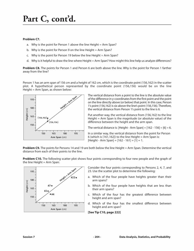
Person 1 has an arm span of 156 cm and a height of 162 cm, which is the coordinate point (156,162) in the scatterplot. A hypothetical person represented by the coordinate point (156,156) would be on the line Height = Arm Span, as shown below:

The vertical distance from a point to the line is the absolute valueof the difference in y-coordinates from the first point and the pointon the line directly above (or below) that point. In this case, Person1’s point (156,162) is six above the line’s point (156,156). Therefore,the vertical distance from Person 1’s point to the line is 6.

Put another way, the vertical distance from (156,162) to the lineHeight = Arm Span is the magnitude (or absolute value) of thedifference between the height and the arm span.

The vertical distance is: |Height - Arm Span| = |162 - 156| = |6| = 6.

In a similar way, the vertical distance from the point for Person6 (which is [161,162]) to the line Height = Arm Span is:|Height - Arm Span| = |162 - 161| = |1| = 1.

Problem C9. The points for Persons 14 and 19 are both below the line Height = Arm Span. Determine the verticaldistance from each of their points to the line.

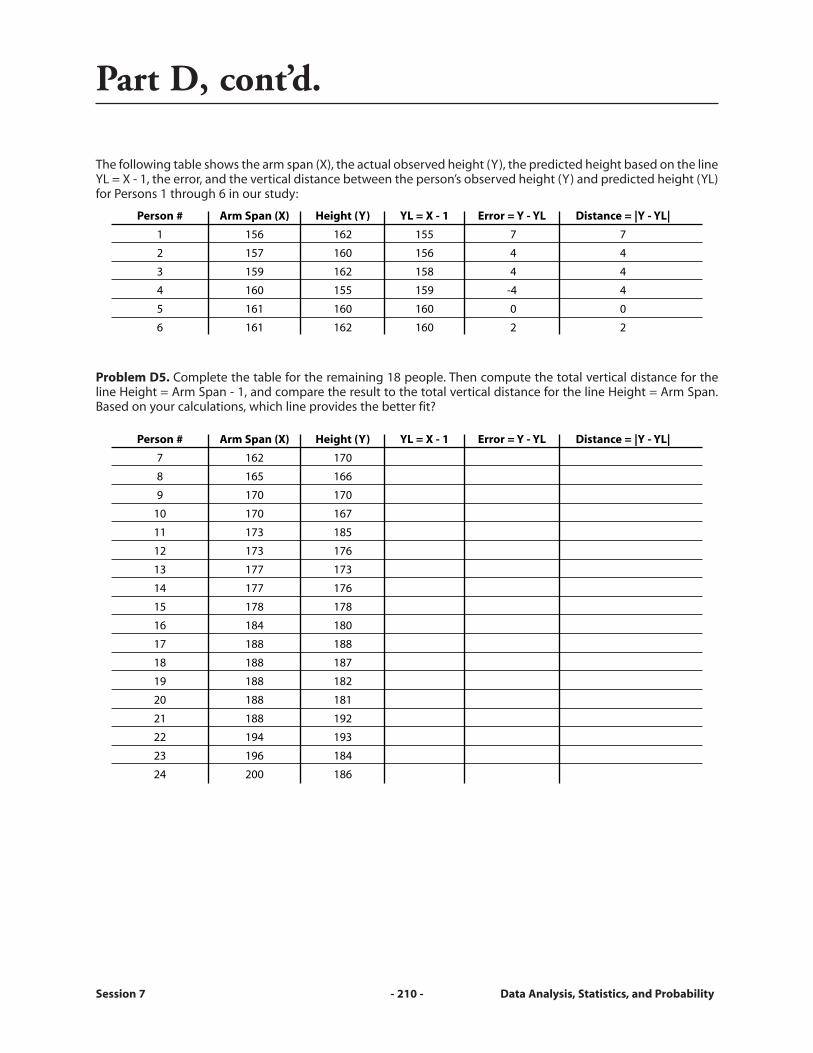
Problem C10. The following scatter plot shows four points corresponding to four new people and the graph ofthe line Height = Arm Span:

Consider the four points corresponding to Persons 2, 4, 7, and23. Use the scatter plot to determine the following:

a. Which of the four people have heights greater than theirarm spans?

b. Which of the four people have heights that are less thantheir arm spans?

c. Which of the four has the greatest difference betweenheight and arm span?

d. Which of the four has the smallest difference betweenheight and arm span?

[See Tip C10, page 222]

Part C, cont’d.


Problem C11. Here is the scatter plot of all 24 people and the graph of the line Height = Arm Span:

Use the scatter plot to help you answer these questions.

a. How many of the 24 people have heights greater than their arm spans?

b. How many of the 24 people have heights less than their arm spans?

c. How many of the 24 people have heights equal to their arm spans?

d. Which three points represent the greatest differences between height and arm span?

e. Other than the points that fall on the line Height = Arm Span, which six points represent the smallest dif-ferences between height and arm span?

Part C, cont’d.

Video Segment (approximate time: 9:00-10:23): You can find this segmenton the session video approximately 9 minutes and 0 seconds after theAnnenberg/CPB logo. Use the video image to locate where to begin viewing.

In this video segment, Professor Kader draws the line Y = X on the class’sscatter plot and asks participants to consider points in relation to this line.


Trend LinesIn Parts A and B, you confirmed that there is a strong positive association between height and arm span—shortpeople tend to have short arms, and tall people tend to have long arms. In Part C, you investigated the nature ofthe relationship between height and arm span by graphing the line Height = Arm Span on a scatter plot of col-lected data. In Part D, using the same data you’ve been working with, you will investigate the use of other lines aspotential models for describing the relationship between height and arm span, and you will explore various cri-teria for selecting the best line.

Again, here is the scatter plot of the 24 people’s data:

Problem D1. Describe the trend in the data points—in other words, how would you describe the general posi-tioning of the points in the scatter plot? What does this trend tell you about the relationship between height andarm span?

Problem D2. Now let’s take another look at the scatter plot with the line Height = Arm Span graphed:

a. Does this line generally provide an accurate description of the trend in the scatter plot?

b. Do you think there might be a better line for describing this trend?

Part D: Fitting Lines to Data (60 minutes)


Problem D3. Let’s consider two other lines for describing the relationship between Height and Arm Span:

• Height = Arm Span + 1

• Height = Arm Span - 1

The following scatter plot includes the graphs of all three lines:

Based on a visual inspec-tion, which of these threelines does the best job ofdescribing the trend in thedata points? Explain whyyou chose this line.

Error

You should have decided in Problem D3 that two of the three lines are better candidates for describing the trendin the data points. The line Height = Arm Span has nine points that are above the line, three that are on the line,and 12 that are below the line. The line Height = Arm Span - 1 has 12 points that are above the line, four that areon the line, and eight that are below the line.

So which of these lines is “better” at describing the relationship? While personal judgement is useful, statisticiansprefer to use more objective methods. To develop criteria for identifying the “better” line, we’ll use a conceptdeveloped in Part C: the vertical distance from a point to a line.

Part D, cont’d.


Person 11, whose arm span is 173 cm and whose height is 185 cm, is represented by the point (173,185) in thescatter plot. If you were to use the line to predict person 11’s height based on his or her arm span, the predictedvalues would be represented by the point (173,173), which lies on the line Height = Arm Span. The scatter plotthus far looks like this:

The difference between the actual observed height (Y) and the corresponding hypothetical, predicted height (onthe line) is called the error. If we use YL (Y on the line) to designate the Y coordinate that represents the predictedheight, then we calculate the error as follows:

Error = Y - YL

In other words, Error = Actual Observed Height - Predicted Height (on the line).

Finally, the vertical distance between an actual height and a hypothetical, predicted height can be expressed as:

Distance = |Y - YL| = |Error|

Let’s see how this works for the line Height = Arm Span (i.e., YL = X).

The following table shows the arm span (X), the actual observed height (Y), the predicted height based on the lineHeight = Arm Span (i.e., YL = X), the error, and the vertical distance between the person’s observed height (Y) andpredicted height (YL) for Persons 1 through 6 in our study:

Part D, cont’d.

Person # Arm Span (X) Height (Y) YL = X Error = Y - YL Distance = |Y - YL|

1 156 162 156 6 6

2 157 160 157 3 3

3 159 162 159 3 3

4 160 155 160 -5 5

5 161 160 161 -1 1

6 161 162 161 1 1


Problem D4. Complete this table for the remaining 18 people.

Here are some observations about this table:

• A point above the line is indicated by a positive value of (Y - YL); this is called a positive error.

• A point below the line is indicated by a negative value of (Y - YL); this is called a negative error.

• A point is on the line when (Y - YL) equals 0, and there is no error.

• The vertical distance from a point to the line YL = X is the absolute value of the error. The smaller this dis-tance is, the closer the actual data point is, vertically, to the line.

One measure of how well a particular line describes the trend in bivariate data is the total of the vertical distances.When comparing two lines, the line with the smaller total of the vertical distances is the “better” line in terms ofhow well it describes the linear relationship between the two variables. For the line Height = Arm Span (i.e., YL = X), this is the sum of the sixth column in the previous two tables combined, which is 100.

But perhaps people aren’t really “square.” Might a better prediction be that height is one centimeter shorter thanarm span? Let’s see how well the line Height = Arm Span - 1 (i.e., YL = X - 1) describes the trend.

Part D, cont’d.

Person # Arm Span (X) Height (Y) YL = X Error =Y - YL Distance =|Y - YL|

7 162 170

8 165 166

9 170 170

10 170 167

11 173 185

12 173 176

13 177 173

14 177 176

15 178 178

16 184 180

17 188 188

18 188 187

19 188 182

20 188 181

21 188 192

22 194 193

23 196 184

24 200 186


The following table shows the arm span (X), the actual observed height (Y), the predicted height based on the lineYL = X - 1, the error, and the vertical distance between the person’s observed height (Y) and predicted height (YL)for Persons 1 through 6 in our study:

Problem D5. Complete the table for the remaining 18 people. Then compute the total vertical distance for theline Height = Arm Span - 1, and compare the result to the total vertical distance for the line Height = Arm Span.Based on your calculations, which line provides the better fit?

Part D, cont’d.

Person # Arm Span (X) Height (Y) YL = X - 1 Error = Y - YL Distance = |Y - YL|

7 162 170

8 165 166

9 170 170

10 170 167

11 173 185

12 173 176

13 177 173

14 177 176

15 178 178

16 184 180

17 188 188

18 188 187

19 188 182

20 188 181

21 188 192

22 194 193

23 196 184

24 200 186


1 156 162 155 7 7

2 157 160 156 4 4

3 159 162 158 4 4

4 160 155 159 -4 4

5 161 160 160 0 0

6 161 162 160 2 2


The SSEAnother way to see how close an individual’s data point is to a line is to square the error. This is similar to how youcalculated the variance in Session 5, where you squared the distances from the mean. Like the absolute value,each squared error produces a positive number. Again, for each individual point, the smaller the squared error, thecloser the actual data point is to the line. Here are the squared errors for Persons 1 through 12:

Problem D6. Complete the table to find the squared error for the remaining 12 people.

Part D, cont’d.

Person # Arm Span (X) Height (Y) YL = X Error = Y - YL (Error)2 = (Y - YL)2

1 156 162 156 6 36

2 157 160 157 3 9

3 159 162 159 3 9

4 160 155 160 -5 25

5 161 160 161 -1 1

6 161 162 161 1 1

7 162 170 162 8 64

8 165 166 165 1 1

9 170 170 170 0 0

10 170 167 170 -3 9

11 173 185 173 12 144

12 173 176 173 3 9


13 177 173

14 177 176

15 178 178

16 184 180

17 188 188

18 188 187

19 188 182

20 188 181

21 188 192

22 194 193

23 196 184

24 200 186


Another measure of how well a particular line describes the relationship in bivariate data is the total of thesquared errors. When comparing two lines, the line with the smaller total of the squared errors is the “better” linein terms of how well it describes the linear relationship between the two variables. For the line Height = Arm Span,this is the sum of the sixth column in the previous two tables, which is 784.

This quantity, the sum of squared errors (SSE), is what statisticians prefer to use when comparing different linesfor potential fit. If you could consider all possible lines, then the one with the smallest SSE is called the leastsquares line; it may also be referred to as the line of best fit.

Before we determine the SSE for the line Height = Arm Span - 1 (i.e., YL = X - 1), let’s take a look at Person 1 andthe line YL = X - 1:


1 156 162 155 7 49

Person 1’s squared error can be represented on the graph as a square with a side whose length is |Y - YL|:

The following is the scatter plot for the data and a graph of the line YL = X - 1.

Note once again that a point above the line is indicated by a positive error, a point below the line is indicated bya negative error; and a point is on the line when the error is 0.

Part D, cont’d.


The following table shows the arm span (X), the observed height (Y), the predicted height based on the lineHeight = Arm Span - 1 (i.e., YL = X - 1), the error, and the vertical distance between the person’s observed height(Y) and predicted height (YL) for Persons 1 through 6 in our study:

Problem D7. Complete the table below for the remaining 18 people. Then compute the sum of the squared errorsfor the line Height = Arm Span - 1, and compare the result to the sum of squared errors for the line Height = ArmSpan. Based on your calculations, which line provides a better fit?

Part D, cont’d.

Person # Arm Span (X) Height (Y) YL = X - 1 Error = Y - YL (Error)2 = (Y - YL)2

1 156 162 155 7 49

2 157 160 156 4 16

3 159 162 158 4 16

4 160 155 159 -4 16

5 161 160 160 0 0

6 161 162 160 2 4


7 162 170

8 165 166

9 170 170

10 170 167

11 173 185

12 173 176

13 177 173

14 177 176

15 178 178

16 184 180

17 188 188

18 188 187

19 188 182

20 188 181

21 188 192

22 194 193

23 196 184

24 200 186


More LinesCan we do better? Recall that for the 24 people in this study, the mean arm span is 175.5 cm and the mean heightis 174.8 cm. Note that the mean arm span is .7 cm longer than the mean height. This suggests that we might trythe line Height = Arm Span - .7 to describe the trend in our bivariate data. Let’s see how this line compares withthe previous models.

Here is the scatter plot of the data and a graph of the line YL = X - .7:

Part D, cont’d.

Video Segment (approximate time 16:44-18:01): You can find this segmenton the session video approximately 16 minutes and 44 seconds after theAnnenberg/CPB logo. Use the video image to locate where to begin viewing.

In this video segment, Professor Kader introduces two rules: the sum of errorsand the sum of squared errors. He explains that these are used to evaluatehow well any given line fits a data set and how well each line can predict thevalue of one variable when the value of the other variable is known.


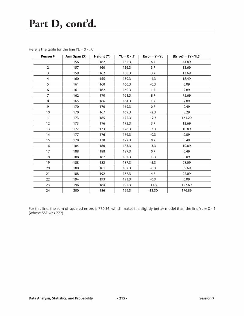
Here is the table for the line YL = X - .7:

For this line, the sum of squared errors is 770.56, which makes it a slightly better model than the line YL = X - 1(whose SSE was 772).

Part D, cont’d.

Person # Arm Span (X) Height (Y) YL = X - .7 Error = Y - YL (Error)2 = (Y - YL)2

1 156 162 155.3 6.7 44.89

2 157 160 156.3 3.7 13.69

3 159 162 158.3 3.7 13.69

4 160 155 159.3 -4.3 18.49

5 161 160 160.3 -0.3 0.09

6 161 162 160.3 1.7 2.89

7 162 170 161.3 8.7 75.69

8 165 166 164.3 1.7 2.89

9 170 170 169.3 0.7 0.49

10 170 167 169.3 -2.3 5.29

11 173 185 172.3 12.7 161.29

12 173 176 172.3 3.7 13.69

13 177 173 176.3 -3.3 10.89

14 177 176 176.3 -0.3 0.09

15 178 178 177.3 0.7 0.49

16 184 180 183.3 -3.3 10.89

17 188 188 187.3 0.7 0.49

18 188 187 187.3 -0.3 0.09

19 188 182 187.3 -5.3 28.09

20 188 181 187.3 -6.3 39.69

21 188 192 187.3 4.7 22.09

22 194 193 193.3 -0.3 0.09

23 196 184 195.3 -11.3 127.69

24 200 186 199.3 -13.30 176.89


Problem D8. Here are the three lines we’ve considered, plus two new ones:

YL = X SSE = 784

YL = X + 1 SSE = 844

YL = X - 1 SSE = 772

YL = X - 2 SSE = 808

YL = X - .7 SSE = 770.56

a. Judging on the basis of the SSE, which is the best line? Which is the worst?

b. What other ways could we change the line equation in an attempt to further reduce the SSE?

c. Is it possible to reduce the SSE to 0? Why or why not?

We have examined several lines that have yielded different SSEs. The lines, however, had one thing in common:They all had a slope of 1, so they were all parallel. Keep in mind that the slope of a line is often described as theratio of rise to run. The formula for slope is: slope = (change in Y) / (change in X). Now, let’s investigate a line witha different slope to describe the trend in the data.

One such line, with slope 0.75, passes through (164, 164) and (188, 182) and near many of the other data points;its equation is YL = 0.75X + 41. Let’s compare this line to line YL = X - .7, which is the best fit we have found so far.

Note that these two lines are not parallel since they have different slopes.

Here is the scatter plot of the 24 people and the graph of the lines YL = .75X + 41 and YL = X - .7:

Part D, cont’d.


Here is the table to find the SSE for the line YL = .75X + 41:

The SSE for the line YL = .75X + 41 is 616.8 (as compared to 770.56). So this new line, with its different slope, turnsout to be a better fit for the data set. [See Note 3]

Part D, cont’d.

Note 3. Fathom Dynamic Statistics Software, used by the participants, is helpful in creating graphical representations of data. If you try theproblems in Part D using Fathom Software, you will be able to test various slopes and intercepts. For more information on Fathom, go to theKey Curriculum Press Web site at www.keypress.com/fathom/.

Person # Arm Span (X) Height (Y) YL = .75X + 41 Error = Y - YL (Error)2 = (Y - YL)2

1 156 162 158 4 16

2 157 160 158.75 1.25 1.5625

3 159 162 160.25 1.75 3.0625

4 160 155 161 -6 36

5 161 160 161.75 -1.75 3.0625

6 161 162 161.75 0.25 0.0625

7 162 170 162.5 7.5 56.25

8 165 166 164.75 1.25 1.5625

9 170 170 168.5 1.5 2.25

10 170 167 168.5 -1.5 2.25

11 173 185 170.75 14.25 203.0625

12 173 176 170.75 5.25 27.5625

13 177 173 173.75 -0.75 0.5625

14 177 176 173.75 2.25 5.0625

15 178 178 174.5 3.5 12.25

16 184 180 179 1 1

17 188 188 182 6 36

18 188 187 182 5 25

19 188 182 182 0 0

20 188 181 182 -1 1

21 188 192 182 10 100

22 194 193 186.5 6.5 42.25

23 196 184 188 -4 16

24 200 186 191 -5 25


SummaryIn this session, we saw how the SSE can be used as cri-teria to determine which line best fits a set of datapoints. The best fit is the line with the smallest SSE. Thisline is referred to as the least squares line because, for agiven set of data points, it is the line that minimizes thesum of the squared errors. In the Interactive Activity onthe course Web site (see box at right), you can see howthese squares can be represented graphically. The leastsquares line is the line that minimizes the total area of allthe squares formed when the vertical distance from thedata points to the line is used as the side lengths of thesquares. [See Note 4]

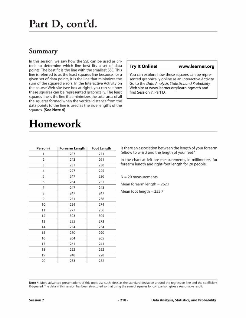
Is there an association between the length of your forearm(elbow to wrist) and the length of your feet?

In the chart at left are measurements, in millimeters, forforearm length and right-foot length for 20 people:

N = 20 measurements

Mean forearm length = 262.1

Mean foot length = 255.7

Part D, cont’d.

Note 4. More advanced presentations of this topic use such ideas as the standard deviation around the regression line and the coefficient R-Squared. The data in this session has been structured so that using the sum of squares for comparison gives a reasonable result.

Try It Online! www.learner.org

You can explore how these squares can be repre-sented graphically online as an Interactive Activity.Go to the Data Analysis, Statistics, and ProbabilityWeb site at www.learner.org/learningmath andfind Session 7, Part D.

Person # Forearm Length Foot Length

1 287 271

2 243 261

3 237 230

4 227 225

5 247 236

6 264 252

7 247 243

8 247 247

9 251 238

10 254 274

11 277 256

12 303 305

13 285 273

14 254 234

15 280 290

16 264 265

17 261 241

18 292 292

19 248 228

20 253 252

Homework


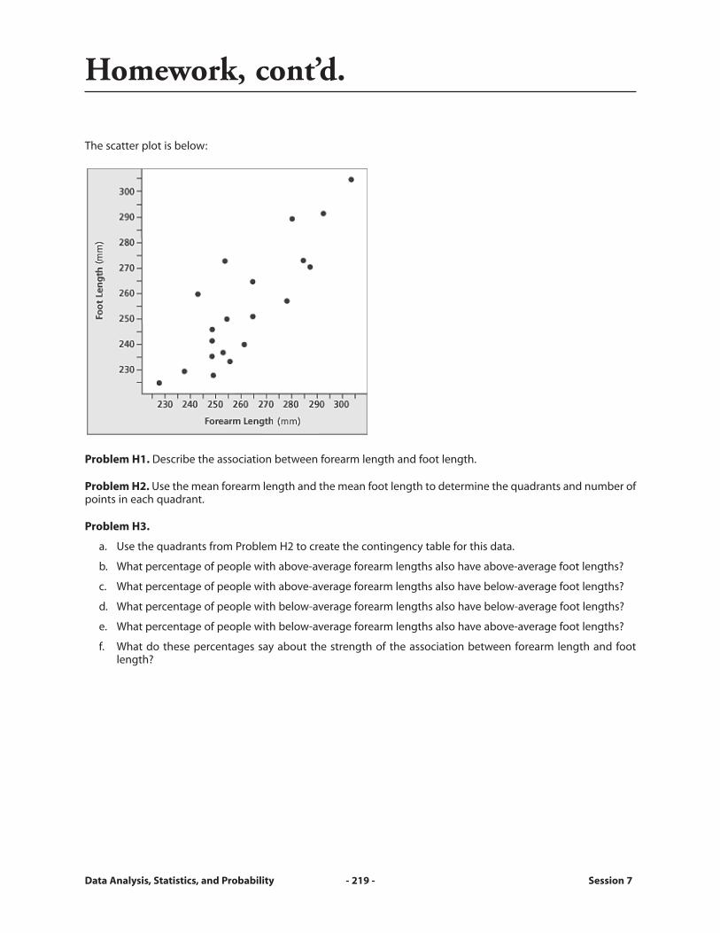
The scatter plot is below:

Problem H1. Describe the association between forearm length and foot length.

Problem H2. Use the mean forearm length and the mean foot length to determine the quadrants and number ofpoints in each quadrant.

Problem H3.

a. Use the quadrants from Problem H2 to create the contingency table for this data.

b. What percentage of people with above-average forearm lengths also have above-average foot lengths?

c. What percentage of people with above-average forearm lengths also have below-average foot lengths?

d. What percentage of people with below-average forearm lengths also have below-average foot lengths?

e. What percentage of people with below-average forearm lengths also have above-average foot lengths?

f. What do these percentages say about the strength of the association between forearm length and footlength?

Homework, cont’d.


Problem H4. Consider the line Foot Length = Forearm Length (i.e., YL = X).

a. Complete the table below.

b. Determine the SSE for this data.

Homework, cont’d.

Person # Forearm Length (X) Foot Length (Y) YL = X Error = Y - YL (Error)2 = (Y - YL)2

1 287 271

2 243 261

3 237 230

4 227 225

5 247 236

6 264 252

7 247 243

8 247 247

9 251 238

10 254 274

11 277 256

12 303 305

13 285 273

14 254 234

15 280 290

16 264 265

17 261 241

18 292 292

19 248 228

20 253 252


Problem H5. Consider the line Foot Length = Forearm Length + 4 (i.e., YL = X + 4).

a. Complete the table below.

b. Determine the SSE for this data.

Problem H6. Compare the SSE in Problem H4 with the SSE in Problem H5. Which line provides a “better” fit?Explain.

Homework, cont’d.

Person # Forearm Length (X) Foot Length (Y) YL = X + 4 Error = Y - YL (Error)2 = (Y - YL)2

1 287 271

2 243 261

3 237 230

4 227 225

5 247 236

6 264 252

7 247 243

8 247 247

9 251 238

10 254 274

11 277 256

12 303 305

13 285 273

14 254 234

15 280 290

16 264 265

17 261 241

18 292 292

19 248 228

20 253 252

Session 7: Tips - 222 - Data Analysis, Statistics, and Probability

Part B: Contingency TablesTip B3. The proportions in the “Above Average” row will be out of 13. Once you find the proportions, use them tofind the percentages.

Part C: Modeling Linear RelationshipsTip C10. Answer questions (c) and (d) by comparing those points to the line Height = Arm Span.

Tips

Data Analysis, Statistics, and Probability - 223 - Session 7: Solutions

Part A: Scatter Plots

Problem A1. No, the data are not sorted by height; for example, the first three heights are 162 cm, 160 cm, and162 cm. However, the data generally appear to be listed in increasing order. The wider we find a person’s arm spanto be, the greater we might expect that person’s height to be, although clearly there is some variation to this rule.The fact that height generally appears in increasing order suggests a positive association between height and armspan.

Problem A2.

a. Answers will vary.

b. Answers will vary, but generally the recorded information should sustain the observation that there is apositive association between height and arm span.

c. Answers will vary.

Problem A3. Yes, there appears to be a positive association. In general, the points in the graph move up and tothe right. There are exceptions to this, but typically, an increase in arm span leads to an increase in height.

Problem A4.

a. Answers will vary.

b. Twelve of the 24 people have above-average arm spans.

c. Thirteen of the 24 people have above-average heights.

d. Eleven people have above-average arm spans and heights. One person has an above-average arm span buta below-average height. Two people have below-average arm spans but above-average heights. Tenpeople have below-average arm spans and heights.

Problem A5. Answers will vary.

Solutions

Session 7: Solutions - 224 - Data Analysis, Statistics, and Probability

Problem A6.

a. No, this will not always happen, because we are considering the mean and not the median. The mean is notnecessarily the median of the data; for example, when considering the heights for this group, we see that13 people are above the mean and 11 are below it.

b. Anyone whose point is to the right of this line has an above-average arm span. In contrast, anyone whosepoint is to the left of the line has a below-average arm span.

Problem A7. Anyone whose point appears above this line has an above-average height. There are 13 such points.

Problem A8. Answers will vary.

Problem A9.

a. People in Quadrant I have above-average arm spans and heights.

b. People in Quadrant II have below-average arm spans and above-average heights.

c. People in Quadrant III have below-average arm spans and heights.

d. People in Quadrant IV have above-average arm spans and below-average heights.

Problem A10.

a. Yes, most people who have above-average arm spans also have above-average heights. By counting thepoints, we can see that 11 of the 12 people with above-average arm spans also have above-average heights.

b. Yes, most people who have below-average arm spans also have below-average heights. By counting thepoints, we can see that 10 of the 12 people with below-average arm spans also have below-averageheights.

Part B: Contingency Tables

Problem B1.

a. Yes. Of the 12 people with below-average arm spans, 10 have below-average heights.

b. Yes. Of the 12 people with above-average arm spans, 11 have above-average heights.

c. These answers suggest a positive association between arm span and height.

Problem B2.

a. Yes. Of the 11 people with below-average heights, 10 have below-average arm spans.

b. Yes. Of the 13 people with above-average heights, 11 have above-average arm spans.

Solutions, cont’d.


Problem B3. Here are the completed tables:

Row proportions:

Row percentages:

Since 90.9% of the people with below-average heights also have below-average arm spans, and 84.6% of thepeople with above-average heights also have above-average arm spans, this again indicates a strong positiveassociation between height and arm span.

Part C: Modeling Linear Relationships

Problem C1. Even though we have established an association, we have not established a description of the natureof the relationship between height and arm span. This question seeks to investigate a specific relationshipbetween arm span and height. Put another way, there are many positive associations (e.g., the associationbetween years of job experience and salary), but the relationship between the variables is not that they are thesame (i.e., “square”).

Problem C2. Answers will vary, but you should generally find the heights and arm spans to be approximately thesame.



Problem C3.

a. It tells you that this person’s height is greater than his or her arm span, and that this person is not “square.”It does not tell you the person’s exact height or arm span.

b. It tells you that this person’s height is less than his or her arm span, and that this person is not “square.”Again, it does not tell you this person’s exact height or arm span.

c. It tells you that this person’s height and arm span are equal, and that this person is “square.”

Problem C4.

a. Two of the five people, Persons 1 and 6, have heights that are greater than their arm spans.

b. Two of the five people, Persons 14 and 19, have heights that are less than their arm spans.

c. Person 19 has the largest difference, 6 cm.

d. Person 9 has the smallest difference, 0 cm. Person 9 is “square.”

Problem C5.

a. Nine people have heights that are greater than their arm spans.

b. Twelve people have heights that are less than their arm spans.

c. Three people have heights that are equal to their arm spans.

d. Persons 5, 6, 8, 14, 18, and 22—the six people with the smallest non-zero difference (±1) in their heights andarm spans—come the closest to being a square without actually being a square.

e. Persons 24, 23, 11, 7, and 20—the people with the greatest difference (positive or negative) between theirheights and arm spans—are the most “non-square.”

Problem C6.

a. Five people have heights and arm spans that differ by more than 6 cm.

b. Nine people have heights and arm spans that differ by less than 3 cm.

Problem C7.

a. Person 1’s height is greater than his or her arm span, so the coordinates of that point will be above the lineHeight = Arm Span.

b. Person 9’s height is equal to his or her arm span, so the coordinates of that point will be on the line Height= Arm Span.

c. Person 19’s height is less than his or her arm span, so the coordinates of that point will be below the lineHeight = Arm Span.

d. Any point on the line Height = Arm Span represents a person who is “square.” Any points that are not onthis line would indicate that a person’s height is either greater or less than that person’s arm span.

Problem C8. Since the difference between height and arm span is greater for Person 1 than it is for Person 6, thepoint for Person 1 should be farther from the line Height = Arm Span than the point for Person 6.

Problem C9. The vertical distance for Person 14 is 1 (|176 - 177| = |-1| = 1). The vertical distance for Person 19 is 6(|182 - 188| = |-6| = 6). In each case the calculation is performed as |Height – Arm Span|.



Problem C10.

a. The points for Persons 2 and 7 are above the line; therefore, their heights are greater than their arm spans.

b. The points for Persons 4 and 23 are below the line; therefore, their heights are less than their arm spans.

c. The point for Person 23 is the farthest from the line, vertically; therefore, Person 23 has the greatest differ-ence between height and arm span.

d. The point for Person 2 is closest to the line, vertically; therefore, Person 2 has the smallest differencebetween height and arm span.

Problem C11.

a. Nine points are above the line, so nine people have heights that are greater than their arm spans.

b. Twelve points are below the line, so 12 people have heights that are less than their arm spans.

c. Three points are on the line, so three people have heights that are equal to their arm spans.

d. The points that are farthest from the line represent people who have the greatest differences betweenheights and arm spans. (These are the points for Persons 11, 23, and 24.)

e. The six points that are closest to the line represent the smallest differences between heights and arm spans.(These are the points for Persons 5, 6, 8, 14, 18, and 22.)

Part D: Fitting Lines to Data

Problem D1. Overall, there is an upward trend; that is, the points generally go up and to the right. This corre-sponds to the positive association between height and arm span.

Problem D2.

a. The line does a reasonably good job. Some points are above the line, some are below it, and some are onthe line, but all are generally pretty close.

b. It looks like it may be possible for another line to be, overall, “closer” to these points.

Problem D3. Answers will vary. The lines Height = Arm Span and Height = Arm Span - 1 each seem to do a goodjob of dividing the points fairly evenly above and below the line, and matching the overall trend of data. It is dif-ficult to distinguish between them without a more mathematical test. Each is clearly better than Height = ArmSpan + 1, which lies above a majority of the points.




Problem D4. Here is the completed table:


For the model YL = X - 1, the total vertical distance is 7 + 4 + … + 13 = 100. Surprisingly, according to this measureof fit, the two lines are equally good. This suggests that another measure of best fit may be useful.

Person # Arm Span (X) Height (Y) YL = X Error = Y - YL Distance = |Y - YL|

7 162 170 162 8 8

8 165 166 165 1 1

9 170 170 170 0 0

10 170 167 170 -3 3

11 173 185 173 12 12

12 173 176 173 3 3

13 177 173 177 -4 4

14 177 176 177 -1 1

15 178 178 178 0 0

16 184 180 184 -4 4

17 188 188 188 0 0

18 188 187 188 -1 1

19 188 182 188 -6 6

20 188 181 188 -7 7

21 188 192 188 4 4

22 194 193 194 -1 1

23 196 184 196 -12 12

24 200 186 200 -14 14


7 162 170 161 9 9

8 165 166 164 2 2

9 170 170 169 1 1

10 170 167 169 -2 2

11 173 185 172 13 13

12 173 176 172 4 4

13 177 173 176 -3 3

14 177 176 176 0 0

15 178 178 177 1 1

16 184 180 183 -3 3

17 188 188 187 1 1

18 188 187 187 0 0

19 188 182 187 -5 5

20 188 181 187 -6 6

21 188 192 187 5 5

22 194 193 193 0 0

23 196 184 195 -11 11

24 200 186 199 -13 13




The sum of squared errors (SSE) is 49 + 16 + … + 169 = 772. Since this is less than the sum of squared errors forthe line Height = Arm Span (which was 784), the line Height = Arm Span - 1 is a slightly better fit.



13 177 173 177 -4 16

14 177 176 177 -1 1

15 178 178 178 0 0

16 184 180 184 -4 16

17 188 188 188 0 0

18 188 187 188 -1 1

19 188 182 188 -6 36

20 188 181 188 -7 49

21 188 192 188 4 16

22 194 193 194 -1 1

23 196 184 196 -12 144

24 200 186 200 -14 196


7 162 170 161 9 81

8 165 166 164 2 4

9 170 170 169 1 1

10 170 167 169 -2 4

11 173 185 172 13 169

12 173 176 172 4 16

13 177 173 176 -3 9

14 177 176 176 0 0

15 178 178 177 1 1

16 184 180 183 -3 9

17 188 188 187 1 1

18 188 187 187 0 0

19 188 182 187 -5 25

20 188 181 187 -6 36

21 188 192 187 5 25

22 194 193 193 0 0

23 196 184 195 -11 121

24 200 186 199 -13 169


Problem D8.

a. The best model is YL = X - .7 because it has the smallest SSE. The worst model is YL = X + 1 because it hasthe largest SSE.

b. As all of these lines have the same slope, if we changed the slope, we might find ways to reduce the SSE.

c. No, we cannot reduce the SSE to 0 unless all the data points lie on a straight line, which these 24 pointsclearly do not do.

Homework

Problem H1. Overall, there is a positive association between forearm length and foot length. On the graph, thepoints generally go up and to the right.

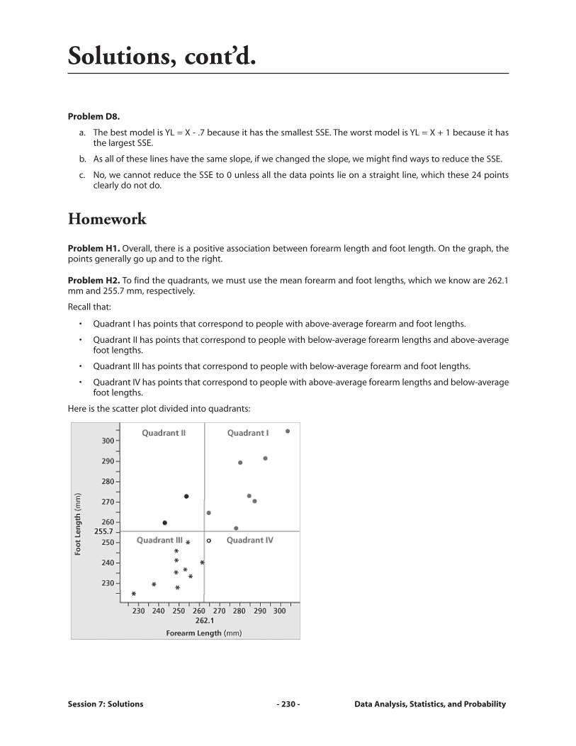
Problem H2. To find the quadrants, we must use the mean forearm and foot lengths, which we know are 262.1mm and 255.7 mm, respectively.

Recall that:

• Quadrant I has points that correspond to people with above-average forearm and foot lengths.

• Quadrant II has points that correspond to people with below-average forearm lengths and above-averagefoot lengths.

• Quadrant III has points that correspond to people with below-average forearm and foot lengths.

• Quadrant IV has points that correspond to people with above-average forearm lengths and below-averagefoot lengths.

Here is the scatter plot divided into quadrants:



Problem H2, cont’d.

This table shows which quadrant each point is in:

Problem H3.

a. The contingency table is at left.

b. Of the eight people with above-average forearm lengths,87.5% (7/8) also have above-average foot lengths.

c. Of the eight people with above-average forearm lengths,only 12.5% (1/8) have below-average foot lengths.

d. Of the 12 people with below-average forearm lengths,83.3% (10/12) also have below-average foot lengths.

e. Of the 11 people with below-average forearm lengths,only 16.7% (2/12) have above-average foot lengths.

f. These percentages say that there is a fairly strong (morethan 80%) positive association between forearm lengthand foot length.


Forearm Foot Length QuadrantLength

287 271 I

243 261 II

237 230 III

227 225 III

247 236 III

264 252 IV

247 243 III

247 247 III

251 238 III

254 274 II

277 256 I

303 305 I

285 273 I

254 234 III

280 290 I

264 265 I

261 241 III

292 292 I

248 228 III

253 252 III


Problem H4.

a. Here is the completed table:

b. The SSE, (256 + 324 + … + 400 + 1), is 3,374.


Person # Forearm Length (X) Foot Length (Y) YL = X Error = Y - YL (Error)2 = (Y - YL)2

1 287 271 287 -16 256

2 243 261 243 18 324

3 237 230 237 -7 49

4 227 225 227 -2 4

5 247 236 247 -11 121

6 264 252 264 -12 144

7 247 243 247 -4 16

8 247 247 247 0 0

9 251 238 251 -13 169

10 254 274 254 20 400

11 277 256 277 -21 441

12 303 305 303 2 4

13 285 273 285 -12 144

14 254 234 254 -20 400

15 280 290 280 10 100

16 264 265 264 1 1

17 261 241 261 -20 400

18 292 292 292 0 0

19 248 228 248 -20 400

20 253 252 253 -1 1


Problem H5.

a. Here is the completed table:

b. The SSE, (400 + 196 + … + 576 + 25), is 4,558.

Problem H6. The first SSE issmaller, which means that the lineFoot Length = Forearm Length is abetter fit to the data than the lineFoot Length = Forearm Length + 4.On the right is an illustration ofthese two lines on top of the dataset:

As you can see from the graph, the line Foot Length= Forearm Length is a closer representation of thedata than the line Foot Length = Forearm Length + 4.


Person # Forearm Length (X) Foot Length (Y) YL = X + 4 Error = Y - YL (Error)2 = (Y - YL)2

1 287 271 291 -20 400

2 243 261 247 14 196

3 237 230 241 -11 121

4 227 225 231 -6 36

5 247 236 251 -15 225

6 264 252 268 -16 256

7 247 243 251 -8 64

8 247 247 251 -4 16

9 251 238 255 -17 289

10 254 274 258 16 256

11 277 256 281 -25 625

12 303 305 307 -2 4

13 285 273 289 -16 256

14 254 234 258 -24 576

15 280 290 284 6 36

16 264 265 268 -3 9

17 261 241 265 -24 576

18 292 292 296 -4 16

19 248 228 252 -24 576

20 253 252 257 -5 25


Notes

session 7 bivariate data and analysis - learner · pdf filesession 7 bivariate data and...

Documents