seminar02 mpe

8/13/2019 Seminar02 MPE

http://slidepdf.com/reader/full/seminar02-mpe 1/7

2. Seminar Energy Methods, FEM Class of 2013

Topic Potential of Internal Energy 24.10.2013

A c c e s s

1 Principal of Minimum of Potential Energy (MPE)

postulation:

Π = Πi + Πe → min (1)

Πi ... internal potential energy stored in the body/system

Πe ... potential energy due to external loads, e.g., body forces, traction forces, etc.

problem definition: find Πi dependent on the deformations and rotations in the elastic body(simplification: static problem, elastic body)

dwi

d

Πi =

V

widV (2)

wi ... volume specific strain energy density

wi =

εx

0

σxdεx +

εy

0

σydεy +

εz

0

σzdεz +

γ xy

0

τ xydγ xy +

γ yz

0

τ yzdγ yz +

γ xz

0

τ xzdγ xz (3)

dwi = σ : dε

with σ =

σx τ xy τ xz

τ yx σy τ yz

τ zx τ zy σz

and ε =

εx1

2γ xy

1

2γ xz

1

2γ yx εy

1

2γ yz

1

2γ zx

1

2γ zy εz

Solution steps

1. chose specific stress condition (e.g. plane stress, plane strain)

2. set stress-strain relationship (e.g. Hooke’s law)

3. set strain-displacement relationship (e.g. truss, beam, linear Bernoulli)

4. find displacement field over the body which leads to minimum potential of the total systemunder consideration of boundary conditions

1



Minimisation (Extremum) Principal

δ Π = δ (Πi + Πe) = 0 (4)

variation: δ (.) = ∂ (.)

∂u · δu with displacement field u

• exact fulfilment of extremum conditions leads to Eulerian differential equations ≡ stronglocal form of equilibrium conditions

• approximate fulfilment of extremum conditions leads to weak form (Ritz-method)

yN (x) = ϕ0 (x) +ni=1

ai · ϕi (x) (5)

yN (x) ... approximation/ansatz-function for displacement

ϕ0 (x) ... function for particular solution u = 0 at ∂ B (boundary)

ϕi (x) ... homogeneous solution function for u = 0 at ∂ B

ai ... unknowns

• requirements:

– yN needs to fulfil kinematic boundary conditions (displacement boundary conditions)

– yN does’nt necessarily satisfy natural boundary conditions (traction boundary condi-tions)

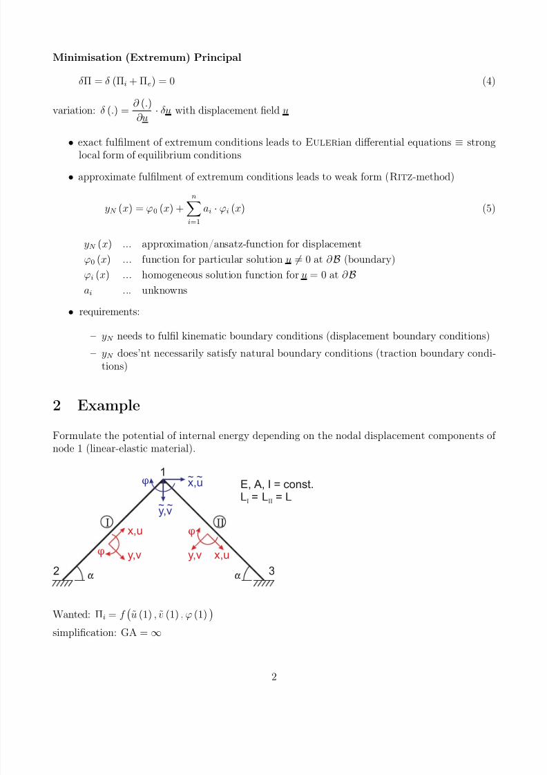
2 Example

Formulate the potential of internal energy depending on the nodal displacement components of node 1 (linear-elastic material).

x,u

y,v

1

2 3

I II

~

x,u

y,v x,uy,v

~ ~

~E, A, I = const.L = L = L

I II

Wanted: Πi = f

u (1) , v (1) , ϕ (1)

simplification: GA = ∞

2



3 Solution

Wanted: internal potential energy for a planar Bernoulli-Beam in form of Πi = f

u (1) , v (1) , ϕ (1)

.

specific stress state (solution step 1)

σx = 0 σy = σz = 0

τ xz = τ xy = 0 (no torsion)τ yz = 0 (no shearing)

stress-strain relationship (solution step 2)

σx = E · εx (6)

internal potential for each beam (in local coordinates):

Πi =

V

εx0

σxd εxd V = E

V

εx0

εxd εxd V = 1

2E

V

ε2xd V (7)

strain-displacement relationship (solution step 3)strains in linear regime (small strains):

εx = d u

d x (8)

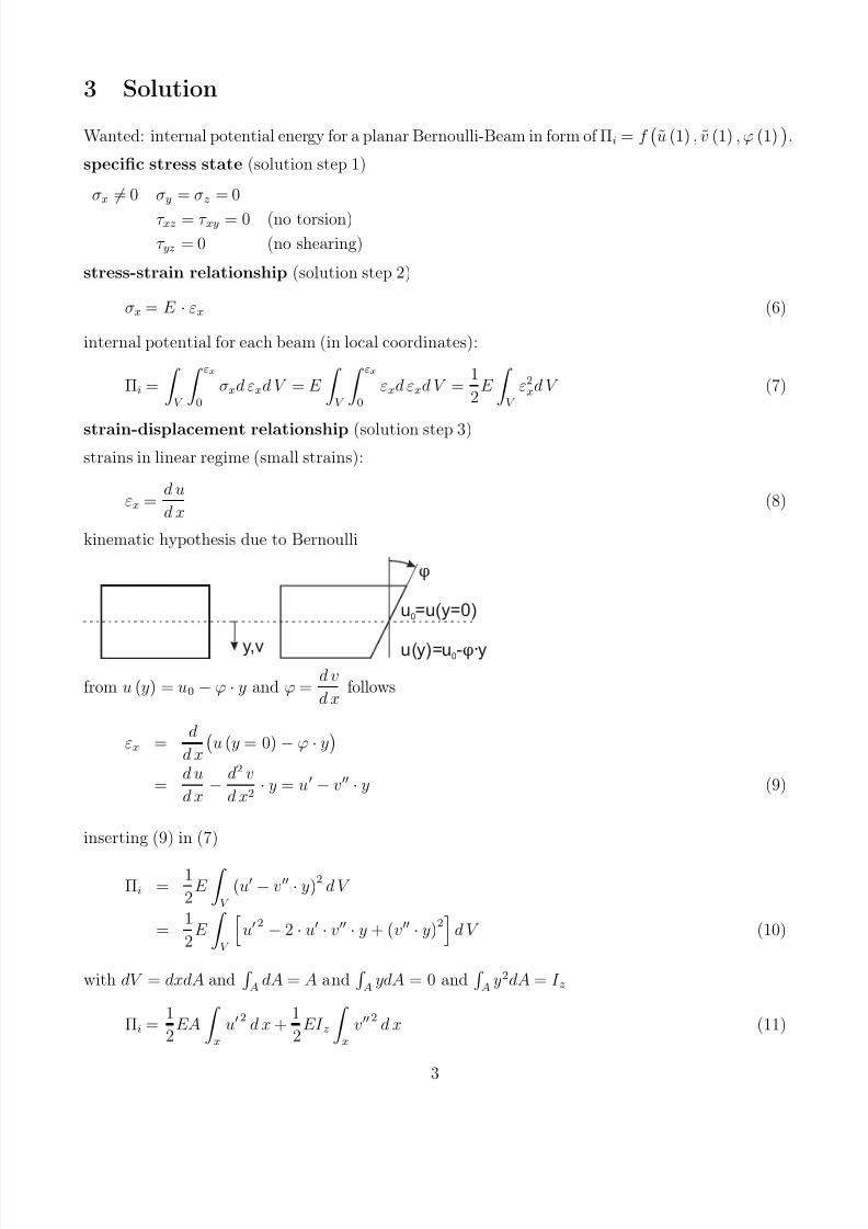
kinematic hypothesis due to Bernoulli

y,v

u =u(y=0)0

u(y)=u - y0

from u (y) = u0 − ϕ · y and ϕ = d v

d x follows

εx = d

d x

u (y = 0)− ϕ · y

=

d u

d x −

d2 v

d x2 · y = u − v · y (9)

inserting (9) in (7)

Πi = 1

2E

V

(u − v · y)2

d V

= 1

2E

V

u 2 − 2 · u · v · y + (v · y)

2

d V (10)

with dV = dxdA and A

dA = A and A

ydA = 0 and A

y2dA = I z

Πi = 1

2EA

x

u 2 d x + 1

2EI z

x

v 2 d x (11)

3



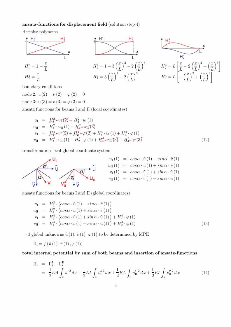
ansatz-functions for displacement field (solution step 4)

Hermite-polynoms

x

1

L

2

1H H

2

2

x

1H

4

3

4

1 H

L

x

H

4

4

4

2

H

L

H 21

= 1− x

L H 4

1 = 1− 3

x

L

2

+ 2x

L

3

H 42

= L

x

L − 2

x

L

2

+x

L

H 22

= x

L H 4

3 = 3

x

L

2

− 2x

L

3

H 44

= L

−x

L

2

+x

L

3

boundary conditions

node 2: u (2) = v (2) = ϕ (2) = 0

node 3: u (3) = v (3) = ϕ (3) = 0

ansatz functions for beams I and II (local coordinates)

uI =

H 21 · uI (2) + H 2

2 · uI (1)

uII = H 21 · uII (1) +

H 22 · uII (3)

vI =

H 41 · vI (2) +

H 42 · ϕ (2) + H 4

3 · vI (1) + H 4

4 · ϕ (1)

vII = H 41 · vII (1) + H 4

2 · ϕ (1) +

H 43 · vII (3) +

H 44 · ϕ (3) (12)

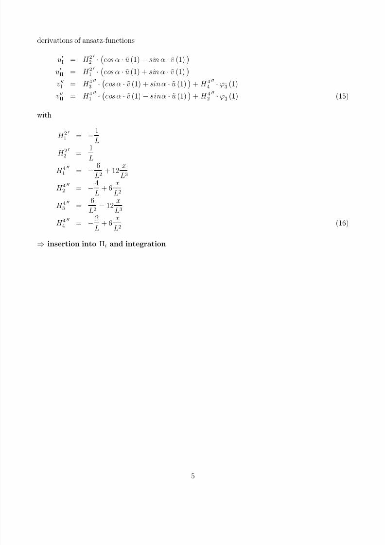
transformation local-global coordinate system

uI

uII

~u

~v

vI

~u

~v

vII

uI (1) = cosα · u (1)− sinα · v (1)

uII (1) = cosα · u (1) + sin α · v (1)

vI (1) = cosα · v (1) + sin α · u (1)vII (1) = cosα · v (1)− sin α · u (1)

ansatz functions for beams I and II (global coordinates)

uI = H 22 ·

cosα · u (1)− sinα · v (1)

uII = H 21 ·

cosα · u (1) + sin α · v (1)

vI = H 43 ·

cosα · v (1) + sin α · u (1)

+ H 44 · ϕ (1)

vII = H 41 · cosα · v (1)− sinα · u (1) + H 4

2 · ϕ (1) (13)

⇒ 3 global unknowns u (1), v (1), ϕ (1) to be determined by MPE

Πi = f (u (1) , v (1) , ϕ (1))

total internal potential by sum of both beams and insertion of ansatz-functions

Πi = ΠI

i + ΠII

i

= 1

2EA

x

u

I

2d x +

1

2EI

x

v

I

2d x +

1

2EA

x

u

II

2d x +

1

2EI

x

v

II

2d x (14)

4



derivations of ansatz-functions

u

I = H 2

2

·

cos α · u (1)− sin α · v (1)

u

II = H 2

1

·

cos α · u (1) + sin α · v (1)

v

I = H 4

3

·

cos α · v (1) + sin α · u (1)

+ H 4

4

· ϕ3 (1)

v

II = H 4

1

· cos α · v (1)− sinα · u (1) + H 4

2

· ϕ3 (1) (15)

with

H 21

= −1

L

H 22

= 1

L

H 41

= − 6

L2 + 12

x

L3

H

4

2

= −

4

L + 6

x

L2

H 43

= 6

L2 − 12

x

L3

H 44

= −2

L + 6

x

L2 (16)

⇒ insertion into Πi and integration

5



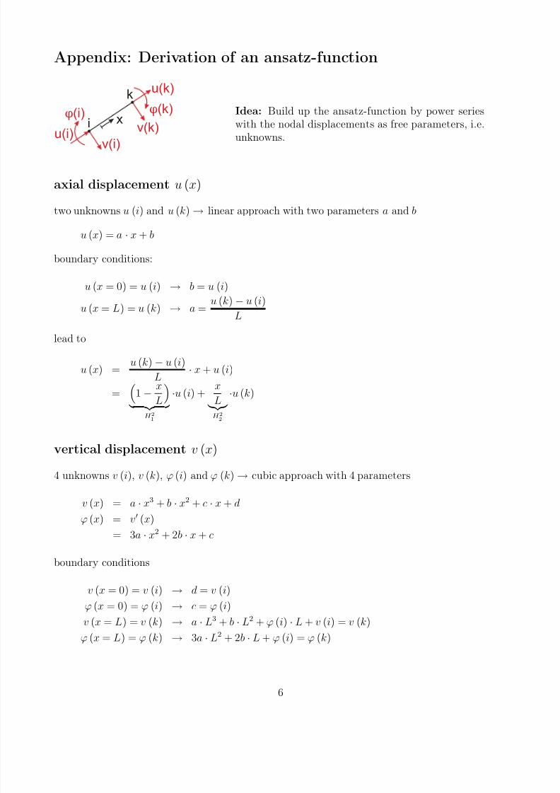
Appendix: Derivation of an ansatz-function

i

k

u(i)

u(k)

v(k)

v(i)

x(i) (k) Idea: Build up the ansatz-function by power serieswith the nodal displacements as free parameters, i.e.

unknowns.

axial displacement u (x)

two unknowns u (i) and u (k) → linear approach with two parameters a and b

u (x) = a · x + b

boundary conditions:

u (x = 0) = u (i) → b = u (i)

u (x = L) = u (k) → a = u (k)− u (i)

L

lead to

u (x) = u (k)− u (i)

L · x + u (i)

=

1− x

L

H

2

1

·u (i) + x

L

H 2

2

·u (k)

vertical displacement v (x)

4 unknowns v (i), v (k), ϕ (i) and ϕ (k) → cubic approach with 4 parameters

v (x) = a · x3 + b · x2 + c · x + d

ϕ (x) = v (x)

= 3a · x2 + 2b · x + c

boundary conditions

v (x = 0) = v (i) → d = v (i)

ϕ (x = 0) = ϕ (i) → c = ϕ (i)

v (x = L) = v (k) → a · L3 + b · L2 + ϕ (i) · L + v (i) = v (k)

ϕ (x = L) = ϕ (k) → 3a · L2 + 2b · L + ϕ (i) = ϕ (k)

6



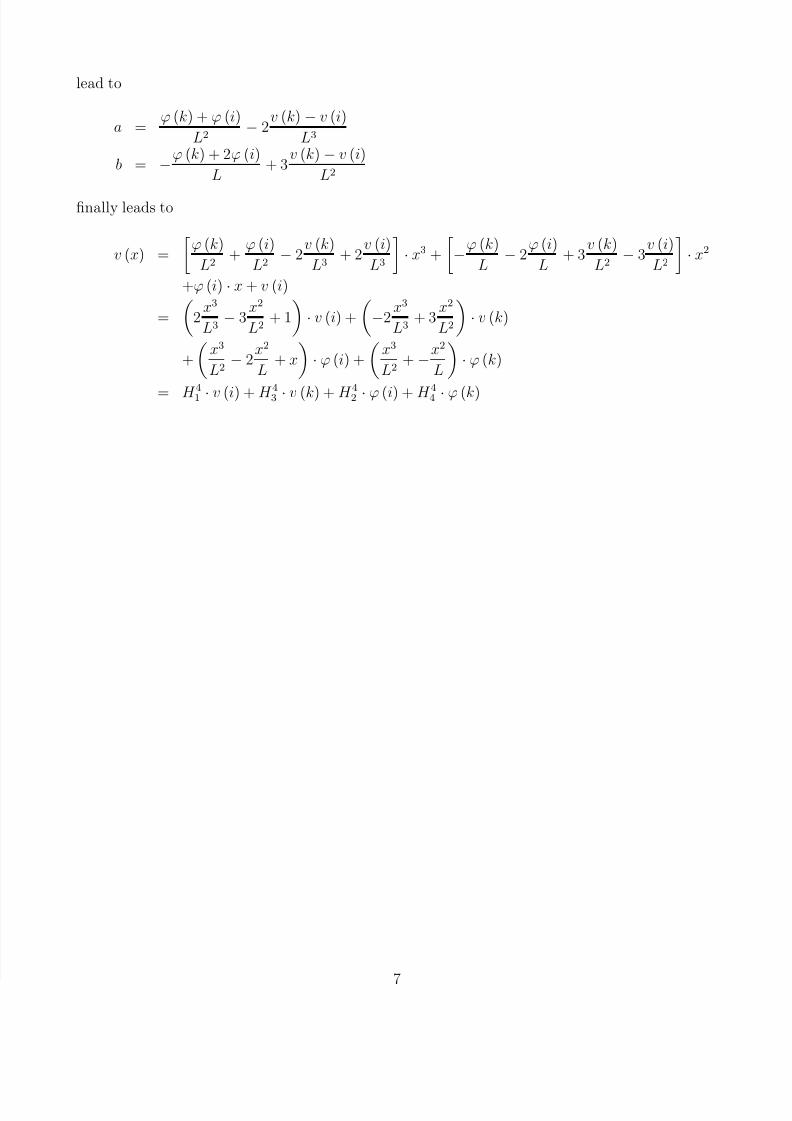
lead to

a = ϕ (k) + ϕ (i)

L2 − 2

v (k) − v (i)

L3

b = −ϕ (k) + 2ϕ (i)

L + 3

v (k)− v (i)

L2

finally leads to

v (x) =

ϕ (k)

L2 +

ϕ (i)

L2 − 2

v (k)

L3 + 2

v (i)

L3

· x3 +

−

ϕ (k)

L − 2

ϕ (i)

L + 3

v (k)

L2 − 3

v (i)

L2

· x2

+ϕ (i) · x + v (i)

=

2

x3

L3 − 3

x2

L2 + 1

· v (i) +

−2

x3

L3 + 3

x2

L2

· v (k)

+

x3

L2 − 2

x2

L + x

· ϕ (i) +

x3

L2 +−

x2

L

· ϕ (k)

= H 4

1 · v (i) + H 4

3 · v (k) + H 4

2 · ϕ (i) + H 4

4 · ϕ (k)

7

seminar02 mpe

Documents