scenario analysis of future pension incomes - gov.uk · scenario analysis of future pension incomes...
TRANSCRIPT
Scenario analysis of future pension incomes
August 2014

Scenario analysis of future pension incomes
Contacts
Contact points for further information:
Press enquiries should be directed to the Department for Work and Pensions press office:
Media Enquiries: 0203 267 5129
Out of hours: 0203 267 5144
Website: https://www.gov.uk/
Follow us on Twitter: www.twitter.com/dwppressoffice
Other enquiries about these statistics should be directed to:
Richard Brookes ([email protected])
ISBN 978-1-78425-302-8
Scenario analysis of future pension incomes
Contents
Executive Summary.................................................................................................... 3
The baseline ............................................................................................................... 6
Updating our estimate of undersaving .................................................................... 6
Investigating factors that can influence undersavers – the “what if” analyses .......... 13
What if employment among people aged 50 and over were higher? .................... 14
What if opt out rates for automatic enrolment were different?............................... 25
What if contribution rates were higher than 8 per cent?........................................ 32
What is the impact of up-rating the new State Pension by earnings? ................... 38
What if the full rate of the New State pension were higher?.................................. 45
Annex A: Selecting the Fuller Working Lives cohort for the employment “what if” analysis .................................................................................................................... 51
Annex B: In-depth focus on contribution rates to Defined Contribution pension schemes ................................................................................................................... 52
Mixed contribution rates ........................................................................................ 58
Annex C: In-depth focus on up-rating of the new State Pension .............................. 62
How reliant are individuals on their State Pension income?.................................. 62
Where do the 1.8 million new undersavers come from? ....................................... 70
Annex D (technical): Methodology and models used to analyse future retirement incomes .................................................................................................................... 72
Annex E: Summary charts of the impact of the “what if” analyses............................ 78

Scenario analysis of future pension incomes
Executive Summary This document builds on work we presented in September 2013 to further explore the factors that impact adequacy of income in retirement.
In September 2013 we introduced a method for assessing the adequacy of people’s retirement incomes, using a replacement rate (a measure of pension income as a percentage of income between age 50 and State Pension age) and target rates derived in the Pensions Commission report of 2004.
This work showed that almost half of adults below State Pension age were not saving enough for their retirement – the key reasons being:
• Not having a full work history, and so having less than full entitlement to the State Pension, and reduced capacity for private pension saving. This was more typical of people in lower income groups;
• Not contributing to private pensions while in work, which was more typical of people in the middle income groups;
• Not contributing enough to private pensions to generate a large enough retirement income, which was more typical of people in the higher income groups.
The September 2013 report also identified the impact that the new “Single Tier” State Pension (now called the “new State Pension”) and automatic enrolment reforms would have on pension adequacy – reducing the number of undersavers by around 1 million, with automatic enrolment practically eliminating the problem of not saving while in work.
The benefits from the new State Pension and automatic enrolment will make noticeable improvements to the pension adequacy of most of the current working-age population. These reforms will provide adequate pensions for many people on lower incomes, providing that they are eligible for a full State Pension.
With the reforms in place, around 92 per cent of undersavers are on the right track to secure an adequate income in retirement, being either “mild” or “moderate” undersavers – some of whom need only a few extra pounds per week in retirement to achieve adequacy. There are still many who need to take positive action to ensure that they have adequate pensions in retirement. This is particularly the case for moderate and high earners.
3

Scenario analysis of future pension incomes
Having a fuller work history and increasing pension contributions can have a substantial impact on the amount of income a person has in retirement. A full work history helps people maintain their standard of living in retirement by ensuring continued contributions and by protecting financial wealth. Increasing pension contributions beyond the automatic enrolment default level is especially important for those on moderate and high income to achieve an adequate pension.
Following on from this work, we have continued to investigate the impact that certain levers can have in a new State Pension and automatic enrolment world on pension adequacy. How do opt out rates from automatic enrolment, employment levels in pre-retirement years, contribution rates, up-rating and the starting value of the new State Pension impact on undersaving?
Figure 1: Overall impact on the percentage of people thought to be undersaving for retirement under each of our policy lever analyses
36%
38%
40%
42%
44%
46%
48%
50%
Perc
enta
ge u
nder
savi
ng
Employment: fuller working lives cohort Opt-out ratesContribution rates New State Pension upratingNew State Pension start rate
Earnings up-rating
Baseline for FWL cohort
40% opt out Moderate uplift Substantial uplift
Triple-lock up-rating
£148.40
10% opt out 15% opt out 8% contributions
£149.10
12% contributions £154.20
15% contributions
The effect of these levers on undersaving is broadly:
• Having a fuller working life between the age of 50 and State Pension age can markedly reduce the risk of undersaving. Additional years contributing to Defined Contribution schemes provide higher pension incomes particularly for medium to high earners. Unlike pension choices that take time to mature (such as opting in to workplace pensions, or increasing contribution rates) having a fuller working life can have a more immediate impact on undersavers;
4

Scenario analysis of future pension incomes
• Replacing the Triple-Lock up-rating guarantee on the State Pension with a simple earnings up-rating would lead to a large increase in the number of undersavers. Over time, the difference between the Triple Lock and earnings growth means that this is particularly an issue for people reaching State Pension age in the 2040’s and beyond;
• Increased opt out rates cause higher levels of undersaving, especially over the long-term future as automatic enrolment matures;
• Those in the middle incomes groups can see huge improvements to their pension adequacy by increasing contribution rates. For those at the very top of the earnings distribution before retirement, private pensions saving at a rate higher than 15 per cent would be needed to achieve an adequate retirement income;
• Each increase in the starting value of the new State Pension by £1 leads to around a 110,000 reduction in the numbers of undersavers, up to a value of £154.20 per week. Undersaver numbers in the middle income groups see the largest reductions;
5

Scenario analysis of future pension incomes
The baseline
Updating our estimate of undersaving
1. In September 2013 the Department for Work and Pensions published the “Framework for the analysis of future pension incomes”, introducing the Department’s methodology for looking at whether people are adequately saving for their retirements, and making an initial estimate of the level of undersaving in the population.
• Around 12.2 million adults below State Pension age were found to be not saving enough for their retirement;
• The introduction of the new State Pension and automatic enrolment into workplace pensions schemes are key factors – without which around an additional 1 million people would be considered undersavers.
2. The undersavers measure that we use takes the ratio of average pension income (average over all years in retirement) to average earnings between age 50 and State Pension age to produce a replacement rate, which is compared with target replacement rates calculated in the Pensions Commission report of 2004.
3. Looking at replacement rates in this way allows us to judge the financial transition a person may experience when moving into retirement. Using the Pensions Commission targets allows us to determine if the transition will allow a person to continue a similar standard of living, or whether they have under-saved for retirement.
4. Further details of the way we construct the undersavers measure can be found in the technical annex.
5. Since the original publication, we have made a number of improvements to the way we model our measure of undersaving; around employment among older workers, occupational pension scheme charges and opt out behaviours under automatic enrolment.
• The way we determine likelihood of employment for older workers has been improved. By using finer alignment among workers aged 50 and over we are able to give a closer reflection of trends;
• We have improved the distribution of scheme charges for private pensions, and introduced a 0.75 per cent charge cap to our modelling;
• We have adopted a lower opt out rate from automatic enrolment following evidence collected from the initial stages of roll out, and improved the modelling of pension choices in Pensim2 following opt out.
6

Scenario analysis of future pension incomes
6. We continue to use the Department’s Pensim2 dynamic micro-simulation model to look at earnings between 50 and State Pension age, and pension incomes from state and private pensions and non-pensions wealth to define each person’s replacement rate. We also retain the five income-related replacement rate targets first set out in the Pensions Commission report of 2004, which we use to categorise individuals according to their average earnings between age 50 and State Pension age.
7. The changes outlined in paragraph 5 provide an estimate of around 11.9 million adults below State Pension age not saving enough to provide an adequate retirement income. The majority of the change from the previous estimate comes from the improved modelling of employment among the over fifties.
8. We can see in Table 1 and Figure 2 below that undersaving is a particular issue for individuals in the middle to higher income groups:
Table 1: Undersavers by Pensions Commission income band
Pensions Commission income band
Number of undersavers
As proportion of Pensions Commission band
As proportion of all undersavers
Band 1 (under £12,300) 0.2m 7% 1%
Band 2 (£12,300 to £22,700) 1.9m 23% 16%
Band 3 (£22,700 to £32,500) 4.2m 52% 35%
Band 4 (£32,500 to £52,000) 4.6m 62% 38%
Band 5 (Over £52,000) 1.1m 67% 10%
Total 11.9m 43% 100%
Note: Tables throughout this publication are rounded to the nearest 100 thousand and the nearest whole percentage point.
7

Scenario analysis of future pension incomes
Figure 2: Undersavers by Pensions Commission income band
0
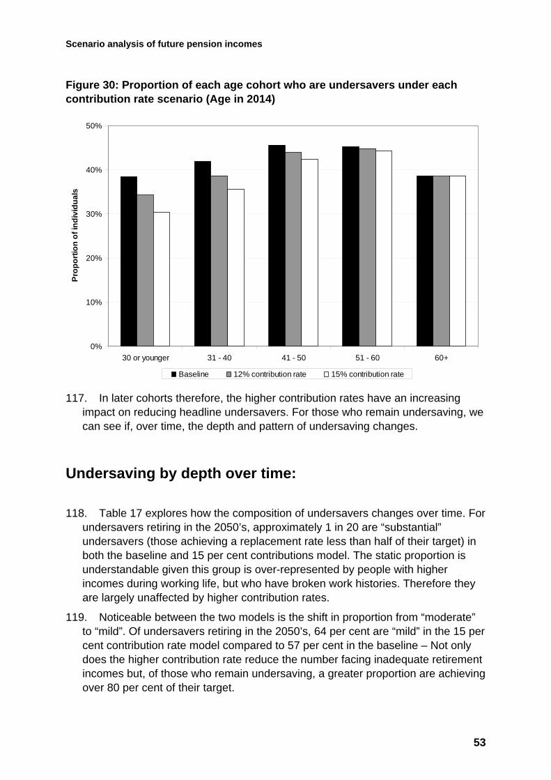
500
1,000
1,500
2,000
2,500
3,000
3,500
4,000
4,500
5,000
Pensions CommissionBand 1
Pensions CommissionBand 2
Pensions CommissionBand 3
Pensions CommissionBand 4
Pensions CommissionBand 5
Num
ber o
f ind
ivid
uals
(tho
usan
ds)
9. A new development in our measurement of undersaving is the concept of depth of
undersaving – while the headline measure focuses solely on achievement of the Pensions Commission targets, the depth measure allows us to look undersavers in terms of how far they are from achieving their target.
10. In Table 2 below, we see the numbers of undersavers in three groups: “substantial undersavers” who achieve less than 50 per cent of their replacement rate target; “modest undersavers” who achieve between 50 and 80 per cent of their target, and “mild undersavers” who achieve over 80 per cent of their target (though as they are still undersavers, they do not reach 100 per cent of their target). Around half of undersavers are in the “mild” group, and only 8 per cent fall into the “substantial undersaving” group.
8

Scenario analysis of future pension incomes
Table 2: Depth of undersaving
Depth of undersaving Number of undersavers
As proportion of all undersavers
Substantial undersaver
(less than 50% of target achieved) 1.0m 8%
Modest undersaver
(50% to 80% of target achieved) 5.1m 43%
Mild undersaver
(over 80% of target achieved) 5.8m 49%
Total 11.9m 100%
11. Figure 3 below shows the broad distribution of the percentage of target replacement rate achieved for both undersavers and adequate savers. Within all three of the depth of undersaving groups we can see that there is a positive skew – undersavers of each type are more likely to be at the top of their group than at the bottom.
12. Looking at both undersavers and adequate savers, we can see that the distribution is almost centred on the 100 per cent target achievement – achieving adequacy but not “over saving” is the generic behaviour that we see.
Figure 3: Distribution of proportion of target replacement rate achieved
0
500
1,000
1,500
2,000
2,500
3,000
3,500
0 - 0
.1
0.1
- 0.2
0.2
- 0.3
0.3
- 0.4
0.4
- 0.5
0.5
- 0.6
0.6
- 0.7
0.7
- 0.8
0.8
- 0.9
0.9
- 1
1 - 1
.1
1.1
- 1.2
1.2
- 1.3
1.3
- 1.4
1.4
- 1.5
1.5
- 1.6
1.6
- 1.7
1.7
- 1.8
1.8
- 1.9
1.9
- 2
2 - 2
.1
2.1
- 2.2
2.2
- 2.3
2.3
- 2.4
2.4
- 2.5
2.5
- 2.6
2.6
- 2.7
2.7
- 2.8
2.8
- 2.9
2.9
- 3
Proportion of target replacement rate achieved
Num
ber o
f ind
ivid
uals
(tho
usan
ds)
Substantial undersavers Moderate undersavers Mild undersavers Adequate savers
9

Scenario analysis of future pension incomes
13. Another angle that we have been investigating, which is particularly useful when looking at the effects of our “what if” analyses, is the impact on different cohorts defined by the year in which they reach State Pension age.
14. Table 3 below shows the undersavers in each decade cohort (2020’s, 2030’s, 2040’s and 2050’s). The patterns that we see here are linked to the introduction of both automatic enrolment in 2012 and the new State Pension in 2016.
15. The initial roll-out of the new State Pension from 2016 brings a small improvement in undersaving, due to the arrangements that have been put in place to prevent individuals losing out during the transition from the current to the new systems. Over time these transitional protections begin to reduce in magnitude as the balance of entitlement to state pensions moves away from the current system to the new system.
16. The introduction of automatic enrolment in 2012 means that more people are saving into workplace pension schemes. The impact on undersaving is seen from around the mid 2030’s, once people have accrued a sufficiently large pension pot to generate a substantial income stream in retirement.
Table 3: Undersavers by State Pension age decade cohort 2020’s to 2050’s
Cohort decade Number of undersavers
As percentage of cohort
As percentage of all undersavers
2020’s 2.7m 45% 22%
2030’s 3.4m 46% 29%
2040’s 2.5m 43% 21%
2050’s 2.5m 39% 21%
17. Looking more broadly than the undersavers figures, there are two key factors that drive a person’s income in retirement: the years they have spent in work (because this provides entitlement to state pensions and facilitates private pension saving) and the years spent contributing to private pensions (more years leads to a greater private pension pot at retirement).
18. Figure 4 below shows the distribution of years between 22 to State Pension age spent in work for both undersavers and adequate savers. We can see that although both undersavers and adequate savers are skewed to the right, this is stronger among adequate savers – the extra time they spend in work helps provide an adequate retirement income.
10

Scenario analysis of future pension incomes
Figure 4: Distribution of years between 22 and State Pension age spent in work by undersavers and adequate savers
0
1,000
2,000
3,000
4,000
5,000
6,000
7,000
Zero Under10%
10% to20%
20% to30%
30% to40%
40% to50%
50% to60%
60% to70%
70% to80%
80% to90%
Over 90%
Percentage of working age spent in work
Num
ber o
f ind
ivid
uals
(tho
usan
ds)
Undersavers Adequate savers 19. Figure 5 below shows the distribution of the number of working years contributing
to a private pension scheme for undersavers and adequate savers. The distribution for adequate savers is more strongly skewed to the right than the undersavers distribution, which peaks in the 80 to 90 per cent contributing group.
11

Scenario analysis of future pension incomes
Figure 5: Distribution of working years spent contributing to private pensions by undersavers and adequate savers
0
500
1,000
1,500
2,000
2,500
3,000
3,500
4,000
Zero Under10%
10% to20%
20% to30%
30% to40%
40% to50%
50% to60%
60% to70%
70% to80%
80% to90%
Over 90%
Percentage of working years individual contributes to private pension
Num
ber o
f ind
ivid
uals
(tho
usan
ds)
Undersavers Adequate savers 20. Our measure of income in retirement takes state and private pensions and a
measure of non-pensions wealth, adjusts for prices, and takes an average over the number of years spent in retirement (see technical annex for more details). We can see the average measure of annual pension income for undersavers and adequate savers across the five Pensions Commission income bands in Table 4:
Table 4: Average (median) of annual pension income measure (2014 earnings terms)
Pensions Commission income band
All individuals Undersavers Adequate savers
Band 1 (under £12,300) £12,600 £6,500 £13,000
Band 2 (£12,300 to £22,700) £14,900 £10,800 £16,100
Band 3 (£22,700 to £32,500) £17,500 £14,500 £21,600
Band 4 (£32,500 to £52,000) £20,800 £17,800 £28,300
Band 5 (Over £52,000) £25,900 £22,100 £38,800
All Bands £17,200 £15,300 £19,200
12

Scenario analysis of future pension incomes
Investigating factors that can influence undersavers – the “what if” analyses
The baseline discussed in the previous chapter uses the Department’s Pensim2 dynamic micro-simulation model to look at the earnings people receive during the latter part of their working lives, and the pension incomes that they receive throughout their retirement.
This modelling process uses a wide array of assumptions, for example around labour market participation, pensions savings choices, and the rules that define state pension incomes. The baseline assumptions allow us to provide a picture of how the world may look “as is”, but altering these assumptions allows us to look at how the world “may be”.
We have undertaken a series of analyses to investigate how our estimate of the number of undersavers changes under alternate assumptions. These “what ifs” analyses cover five questions:
• What if there were an increase in the level of labour market participation among people aged 50 and over?
• What if opt out rates from automatic enrolment were different?
• What if people paying into Defined Contribution schemes contributed more?
• What if the new State Pension (when it is introduced in 2016) were up-rated by earnings growth rather than the triple lock?
• What if the full starting value of the new State Pension were higher?
Over the next few chapters, we will present the high-level results from modelling each of these questions. We will address findings such as the number of undersavers, which part of the income distribution is affected, how the depth of undersaving changes, and what impacts each has on future cohorts of pensioners.
Two of the “what ifs” are examined in greater detail in annexes to the main research paper. These “what ifs” cause the largest changes in the level of undersaving: the level of contributions that are made into Defined Contribution pension schemes, and the up-rating regime used to yearly revalue the new State Pension when it arrives in 2016.
13

Scenario analysis of future pension incomes
What if employment among people aged 50 and over were higher?
Description of the scenario area:
21. Being in work is a vital part of private pensions saving. Access to workplace pension schemes allows individuals to benefit from not only their own contributions, but also any contribution from their employer and the tax relief that pension saving brings. Since the introduction of automatic enrolment in 2012, the coverage of workplace pensions has increased, further cementing the link between employment and pension saving.
22. Our baseline assumption uses alignment factors derived from the Office for Budgetary Responsibility’s cohort employment model. Separate factors are applied to those aged 50 to 54 and those aged 55 to State Pension age.
23. Our “what if” looks at two alternative assumptions, built around the notion of raising the employment rate in particular age groups to “close the gap” with the immediately younger age group:
• A “modest” rise in employment – the employment rate for people aged 55 to State Pension age is raised to close the gap with those aged 50 to 54 by half and the rate for people aged 50 to 54 is then raised to close the gap with those aged 41 to 49 by half;
• A “substantial” rise in employment – the rates for both 50 to 54 and 55 to State Pension age groups are raised to equal the rate among those aged 41 to 49 (essentially a scenario in which there is no drop-off in employment between age 49 and State Pension age).
24. We assume that there is sufficient labour market demand to accommodate this increase in employment among older workers, and consequently no reduction in employment across other age groups. We do not aim to qualify the causes of the rise in employment modelled, rather look at the adequacy response to such changes.
Key direct impacts:
25. The key impact of the employment scenarios is clearly the amount of time an individual spends in work, which has an impact on both the 50 to State Pension age income and retirement income parts of the replacement rate calculation.
14

Scenario analysis of future pension incomes
26. Figure 6 below shows the impact on the distribution of years of between age 22 and State Pension age spent in work. We can clearly see the shift to the right of the distribution under the higher employment assumptions. The additional years in work mean that individuals can both accrue more state pension entitlement and increase the size of any private pension entitlement (provided that they remain enrolled in a pension scheme and do not draw down that pension income before retirement).
Figure 6: Distribution of years between age 22 and State Pension age spent in work under each scenario (percentage of all individuals)
0%
10%
20%
30%
40%
50%
60%
Zero Under10%
10% to20%
20% to30%
30% to40%
40% to50%
50% to60%
60% to70%
70% to80%
80% to90%
Over 90%
Proportion of working age spent in work
Perc
enta
ge o
f all
indi
vidu
als
Baseline Modest uplift Substantial uplift
27. Not all individuals experience additional years in work under the two employment scenarios – while the likelihood of being in work after the age of 50 is increased the model does not compel individuals to spend more time in work. To better explore the adequacy impact of a fuller working life, we restrict the analysis in the remainder of this “what if” chapter to those individuals who have some working years between 50 and State Pension age in the baseline and who have more working years under the two employment scenarios. The details of this subgroup can be found in annex A.
Headline changes:
28. Looking at those individuals with fuller working lives as set out in annex A, Figure 7 shows the additional years in work between 50 and State Pension age as a result of the alternate employment scenarios. In the “modest” scenario 8 million
15

Scenario analysis of future pension incomes
individuals see between 1 to 5 years of additional work. The “substantial” uplift generates greater shifts; 1 million individuals see an increase of 11 to 15 years additional work between 50 and State Pension age.
Figure 7: Additional Years in work between 50 and State Pension age relative to the baseline
0
1,000
2,000
3,000
4,000
5,000
6,000
7,000
8,000
9,000
1 to 5 years 6 to 10 years 11 to 15 years Above 15 years
Additional years in work between 50-SPa
Num
ber o
f ind
ivid
uals
(tho
usan
ds)
Modest Uplift Substantial uplift
29. With additional years in work, individuals are in a better position to build private pensions. Figure 8 shows the distribution of years saving to a pension between 50 and State Pension age. We can see that additional years in work translate into additional years contributing to a pension.
16

Scenario analysis of future pension incomes
Figure 8: Years contributing to a pension between 50 and State Pension age
0
500
1,000
1,500
2,000
2,500
3,000
3,500
zero 1 to 2 years 3 to 4 years 5 to 6 years 7 to 8 years 9 to 10years
11 to 12years
13 to 14years
Above 14years
Years pension saving between 50 and State Pension age
Num
ber o
f ind
ivid
uals
(tho
usan
ds)
Baseline Modest uplift Substantial uplift
30. Changes in years spent in work and saving in private pensions affect the levels of the income measures in our replacement rate calculation. Figure 9 shows the distribution of the working life income measure amongst the fuller working lives subgroup. We can see how the “substantial” uplift shifts the distribution to the right – additional years in work leads to higher average incomes between age 50 and State Pension age.
17

Scenario analysis of future pension incomes
Figure 9: Distribution of 50 to State Pension age income measure (2014 earnings terms)
0
200
400
600
800
1,000
1,200
1,400
1,600
1,800
2,000
Under£5,000
£5,000 to£10,000
£10,000to
£15,000
£15,000to
£20,000
£20,000to
£25,000
£25,000to
£30,000
£30,000to
£35,000
£35,000to
£40,000
£40,000to
£45,000
£45,000to
£50,000
Over£50,000
Working age income measure (50 to State Pension age average annual earnings)
Num
ber o
f ind
ivid
uals
(tho
usan
ds)
Baseline Substantial uplift
31. In terms of undersaving, a higher working life income requires a related increase in pension income in order for an individual to maintain their replacement rate, and larger still to bring undersavers into adequacy.
32. Figure 10 shows the distribution of the retirement income measure in our replacement rate calculation. Similar to the working life income, the retirement income distribution shifts to the right.
18

Scenario analysis of future pension incomes
Figure 10: Distribution of retirement income measure (2014 earnings terms)
0
500
1,000
1,500
2,000
2,500
3,000
3,500
Under£5,000
£5,000 to£10,000
£10,000to
£15,000
£15,000to
£20,000
£20,000to
£25,000
£25,000to
£30,000
£30,000to
£35,000
£35,000to
£40,000
£40,000to
£45,000
£45,000to
£50,000
Over£50,000
Retirement income measure
Num
ber o
f ind
ivid
uals
(tho
usan
ds)
Baseline Substantial uplift 33. Figure 11 confirms this link by showing the median change in individuals’ pension
pot totals from the baseline scenario across Defined Contribution workplace pension schemes and personal pension schemes.
34. Looking at the secondary (right-hand side) axis, you can see the positive correlation between additional years in work and additional private pension provision.
35. Higher retirement incomes are being driven by increased years in work and more years contributing which, in turn, allow for larger private pension pots to be built-up.
19

Scenario analysis of future pension incomes
Figure 11: Average increase in total pension pot funds relative to the baseline
0
1,000
2,000
3,000
4,000
5,000
6,000
7,000
8,000
9,000
10,000
1 to 5 years 6 to 10 years 11 to 15 years Above 15 years
Additional years in work between 50 and State Pension age
Num
ber o
f ind
ivid
uals
(tho
usan
ds)
£0
£4,000
£8,000
£12,000
£16,000
£20,000
Med
ian
chan
ge in
tota
l pen
sion
s po
t
Modest Uplift Substantial uplift Modest - potsize Substantial - potsize Note: There is only a very small number of individuals in the “above 15 years” group under the modest uplift scenario, as such the estimate of increase in pot funds for these individuals is subject to a higher degree of uncertainty.
36. Table 5 below shows the high-level number and percentage of people thought to be undersaving for retirement amongst the fuller working lives subgroup. Working and contributing for additional years has reduced the proportion of this group projected to experience inadequate retirement incomes by 3 percentage points.
Table 5: Total level of undersaving
Scenario Population Number of undersavers
Change from baseline (individuals)
Undersaver proportion of population
Baseline 10.1m 4.6m - 46%
Modest uplift 10.1m 4.4m -250k 43%
Substantial uplift 10.1m 4.3m -320k 43%
20
Scenario analysis of future pension incomes
Undersaving by income band:
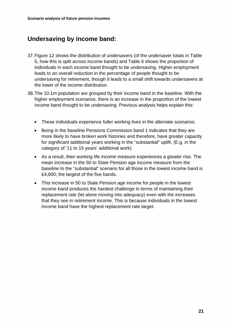
37. Figure 12 shows the distribution of undersavers (of the undersaver totals in Table 5, how this is split across income bands) and Table 6 shows the proportion of individuals in each income band thought to be undersaving. Higher employment leads to an overall reduction in the percentage of people thought to be undersaving for retirement, though it leads to a small shift towards undersavers at the lower of the income distribution.
38. The 10.1m population are grouped by their income band in the baseline. With the higher employment scenarios, there is an increase in the proportion of the lowest income band thought to be undersaving. Previous analysis helps explain this:
• These individuals experience fuller working lives in the alternate scenarios.
• Being in the baseline Pensions Commission band 1 indicates that they are more likely to have broken work histories and therefore, have greater capacity for significant additional years working in the “substantial” uplift. (E.g. in the category of ‘11 to 15 years’ additional work)
• As a result, their working life income measure experiences a greater rise. The mean increase in the 50 to State Pension age income measure from the baseline to the “substantial” scenario for all those in the lowest income band is £4,600; the largest of the five bands.
• This increase in 50 to State Pension age income for people in the lowest income band produces the hardest challenge in terms of maintaining their replacement rate (let alone moving into adequacy) even with the increases that they see in retirement income. This is because individuals in the lowest income band have the highest replacement rate target.
21

Scenario analysis of future pension incomes
Figure 12: Distribution of undersavers across Pensions Commission income bands
0
200
400
600
800
1,000
1,200
1,400
1,600
1,800
Pensions Commission Band1
Pensions Commission Band2
Pensions Commission Band3
Pensions Commission Band4
Pensions Commission Band5
Num
ber o
f und
ersa
vers
(tho
usan
ds)
Baseline Modest uplift Substantial uplift
Table 6: Percentage of each Pensions Commission income band undersaving
Scenario Band 1 (under £12,300)
Band 2 (£12,300 to £22,700)
Band 3 (£22,700 to £32,500)
Band 4 (£32,500 to £52,000)
Band 5 (over £52,000)
Baseline 7% 25% 57% 69% 74%
Modest uplift 16% 25% 50% 65% 70%
Substantial uplift
17% 25% 49% 63% 68%
Undersavers by depth of undersaving:
39. Figure 13 below shows the percentage of undersavers in each “depth of undersaving” group. We can see that not only do the higher employment scenarios reduce headline undersavers (Table 6) but of those remaining undersavers, a higher proportion are closer to their target. For instance, in the “substantial” uplift 53 per cent of the 4.3m undersavers are “mild” compared to 48 per cent of the 4.6m in the baseline.
22

Scenario analysis of future pension incomes
Figure 13: Undersavers by depth of undersaving group
0%
10%
20%
30%
40%
50%
60%
Under 50% - substantial undersaver 50% to 80% - moderate undersaver 80% to 100% - mild undersaverDepth of undersaving group (percentage of target replacement rate achieved)
Perc
enta
ge o
f tot
al u
nder
save
rs in
eac
h de
pth
grou
p
Baseline Modest uplift Substantial uplift
Cohort impacts:
40. Figure 14 below shows the proportion of undersavers in four cohorts defined by the decade in which individuals reach State Pension age. We can see how, among our fuller working lives subgroup, the higher employment scenarios have an impact across all cohorts. Unlike actions affecting an individual’s private pension saving (increasing participation or increasing contributions) or actions that influence the value of the State Pension, changes in employment can have a more immediate impact; indeed the 2020’s cohort sees the largest reduction in undersaver proportions.
23

Scenario analysis of future pension incomes
Figure 14: Proportion of undersavers by State Pension age decade cohort
0%
10%
20%
30%
40%
50%
2020's 2030's 2040's 2050's
Decade individual reaches State Pension age
Perc
enta
ge o
f eac
h co
hort
who
are
und
ersa
vers
Baseline Modest uplift Substantial uplift
41. In summary, alternate assumptions around the employment rate for people aged 50 and over have the following effects:
• An improvement in work history, providing a general rise in both 50 to State Pension age and pension incomes;
• A reduction in the level of undersaving – including a reduction in the undersaving amongst the earliest cohorts to reach State Pension age;
• A slight increase in the level of undersaving at the lower end of the income distribution because increased 50 to State Pension age income makes it harder to achieve adequacy.
24

Scenario analysis of future pension incomes
What if opt out rates for automatic enrolment were different?
Description of the scenario area:
42. From October 2012 the programme of automatic enrolment began to roll out, starting with the largest employers, with all employers subject to the new duties from 2018. Employers are required to automatically enrol eligible workers into a qualifying workplace pension scheme. Workers will be eligible provided they are aged at least 22 and under State Pension age, and earn over the equivalent of £10,000 per year in 2014/15 terms. Individuals have the right to opt out.
43. Within Pensim2, our baseline assumption is a 15 per cent opt out rate for workplace pension schemes. The original programme assumption was for an opt out rate of around 30 per cent, which was based on survey data collected prior to the onset of automatic enrolment about individuals intentions to remain within a pension scheme1. Recent DWP research among larger employers has found that opt out rates were much lower than our earlier assumption2. The opt out assumption was revised to an average of 15 per cent for the life of the programme to reflect these new findings3.
44. Our “what if” looks at two alternative scenarios:
• Opt out rate of 40 per cent – a substantial reduction in participation;
• Opt out rate of 10 per cent – a small increase in participation for workplace pension schemes, leading to more and larger private pensions in the future.
45. Changes in participation in workplace pension saving will have an impact on the net take-home pay of individuals while in work, the cost of contributions for employers and the tax revenues to the Exchequer. These impacts are not quantified as part of this analysis.
1 Bourne T, Shaw A, and Butt S, 2010, Individuals’ attitudes and likely reactions to the workplace pension reforms 2009: Report of a quantitative survey. DWP Research Report No 669. 2 https://www.gov.uk/government/publications/employers-pension-provision-survey-2013-preliminary-findings 3 DWP 11 April 2014 https://www.gov.uk/government/news/pensions-savings-9-million-newly-saving-or-saving-more-says-pensions-minister
25

Scenario analysis of future pension incomes
Key direct impacts:
46. Making changes to the opt out rate will primarily affect those individuals who are in work and whose earnings are sufficient to bring them over the earnings threshold for automatic enrolment. The key change will be in the number of years each individual contributes to a workplace pension scheme.
47. Figure 15 below shows the distribution of the number of working years contributing to a workplace pension scheme for all individuals across different opt out scenarios. With a lower opt out rate, the distribution is more strongly skewed to the right. Relative to the baseline, the 40 per cent opt out model sees nearly 2 million fewer individuals spending over 80 per cent of their working lives contributing.
Figure 15: Change in number of years contributing to workplace pension schemes under each scenario (all individuals)
0
1000
2000
3000
4000
5000
6000
7000
Zero Under10%
10% to20%
20% to30%
30% to40%
40% to50%
50% to60%
60% to70%
70% to80%
80% to90%
Over90%
Percentage of working years individual contributes to private pension
Num
ber o
f ind
ivid
uals
(000
's)
Baseline 10% opt out 40% opt out
Headline changes:
48. Table 7 below shows the high-level number and percentage of people thought to be undersaving for retirement. Under the 10 per cent opt out rate scenario, there
26

Scenario analysis of future pension incomes
is only a small (and negligible) reduction in the number of undersavers of 40 thousand. Owing to the fact that 10 per cent opt out is the smaller of the two deviations from the baseline scenario.
Table 7: Total level of undersaving
Scenario Number of undersavers
As proportion of all individuals
Change from baseline (number)
Baseline 11.9m 43% -
10% opt out 11.9m 43% <50k
40% opt out 12.2m 44% +300k
Undersaving by income band:
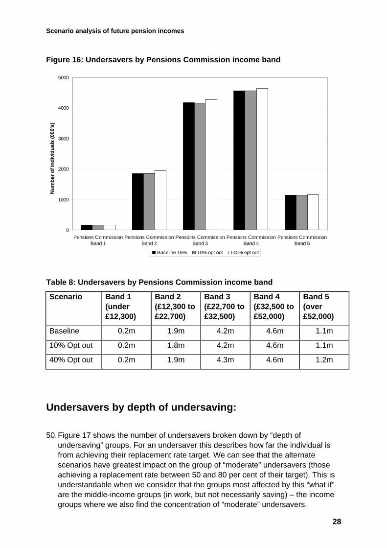
49. Figure 16 and Table 8 below show the impact of the scenarios on the five Pensions Commission income bands. Changes in opt out rate have the following high-level impacts:
• Middle earners see the greatest change in undersaving – they are in stable work and have earnings that bring them into automatic enrolment;
• Low earners are largely unaffected – longer periods out of the labour market mean that they have less opportunity to contribute to workplace pensions;
• High earners typically have good participation in workplace pensions and are less affected by aggregate opt out assumptions.
27
Scenario analysis of future pension incomes
Figure 16: Undersavers by Pensions Commission income band
0
1000
2000
3000
4000
5000
Pensions CommissionBand 1
Pensions CommissionBand 2
Pensions CommissionBand 3
Pensions CommissionBand 4
Pensions CommissionBand 5
Num
ber o
f ind
ivid
uals
(000
's)
Baseline 15% 10% opt out 40% opt out
Table 8: Undersavers by Pensions Commission income band
Scenario Band 1 (under £12,300)
Band 2 (£12,300 to £22,700)
Band 3 (£22,700 to £32,500)
Band 4 (£32,500 to £52,000)
Band 5 (over £52,000)
Baseline 0.2m 1.9m 4.2m 4.6m 1.1m
10% Opt out 0.2m 1.8m 4.2m 4.6m 1.1m
40% Opt out 0.2m 1.9m 4.3m 4.6m 1.2m
Undersavers by depth of undersaving:
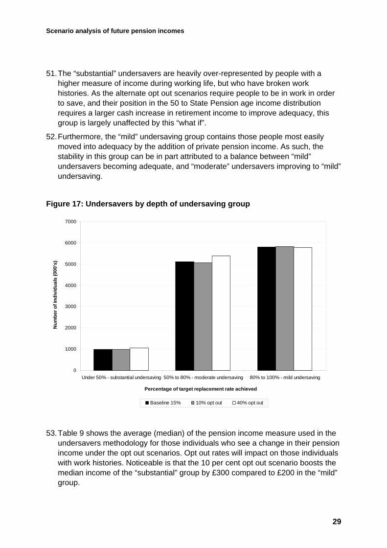
50. Figure 17 shows the number of undersavers broken down by “depth of undersaving” groups. For an undersaver this describes how far the individual is from achieving their replacement rate target. We can see that the alternate scenarios have greatest impact on the group of “moderate” undersavers (those achieving a replacement rate between 50 and 80 per cent of their target). This is understandable when we consider that the groups most affected by this “what if” are the middle-income groups (in work, but not necessarily saving) – the income groups where we also find the concentration of “moderate” undersavers.
28
Scenario analysis of future pension incomes
51. The “substantial” undersavers are heavily over-represented by people with a higher measure of income during working life, but who have broken work histories. As the alternate opt out scenarios require people to be in work in order to save, and their position in the 50 to State Pension age income distribution requires a larger cash increase in retirement income to improve adequacy, this group is largely unaffected by this “what if”.
52. Furthermore, the “mild” undersaving group contains those people most easily moved into adequacy by the addition of private pension income. As such, the stability in this group can be in part attributed to a balance between “mild” undersavers becoming adequate, and “moderate” undersavers improving to “mild” undersaving.
Figure 17: Undersavers by depth of undersaving group
0
1000
2000
3000
4000
5000
6000
7000
Under 50% - substantial undersaving 50% to 80% - moderate undersaving 80% to 100% - mild undersaving
Num
ber o
f ind
ivid
uals
(000
's)
Percentage of target replacement rate achieved
Baseline 15% 10% opt out 40% opt out
53. Table 9 shows the average (median) of the pension income measure used in the undersavers methodology for those individuals who see a change in their pension income under the opt out scenarios. Opt out rates will impact on those individuals with work histories. Noticeable is that the 10 per cent opt out scenario boosts the median income of the “substantial” group by £300 compared to £200 in the “mild” group.
29

Scenario analysis of future pension incomes
• The ”mild” undersaver group has a larger composition of individuals with substantial work and contribution histories in the baseline, therefore they’re already saving.
• “Substantial” undersavers are more likely to be individuals with broken work histories, or people with work histories but who did not contribute. Therefore, the lower opt out rate has the direct impact of modelling some of the baseline non-savers as savers.
Table 9: Average (median) annual pension income by depth of undersaving group for those individuals who see a change in pension income under each opt out scenario (2014 earnings terms)
Scenario Average (median) pension income of undersavers
Among “substantial” undersavers (under 50% target achieved)
Among “moderate” undersavers (50% - 80% target achieved)
Among “mild” undersavers (80% - 100% target achieved)
Baseline (those affected by 10% scenario)
£16,300 £11,200 £15,300 £17,700
10% opt out (those affected)
£16,600 £11,500 £15,500 £17,900
Baseline (those affected by 40% scenario)
£16,200 £11,200 £14,900 £17,500
40% opt out (those affected)
£15,800 £10,900 £14,600 £17,100
Cohort impacts:
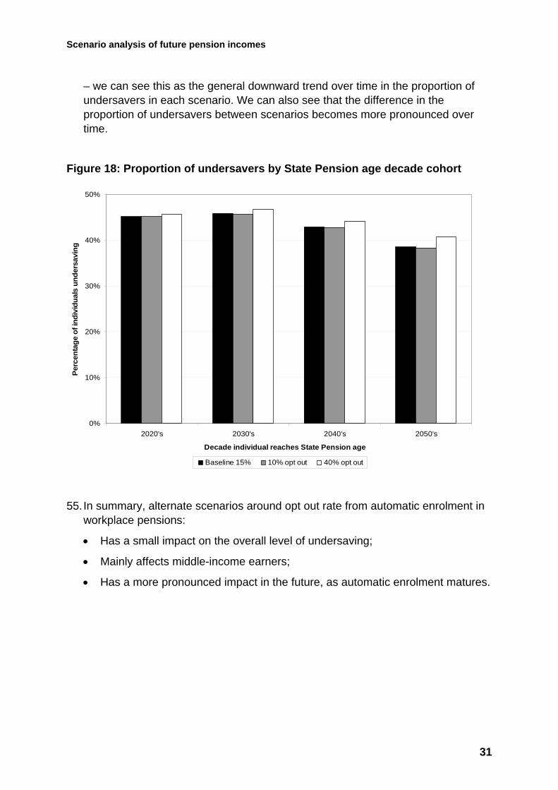
54. Figure 18 below shows the proportion of undersavers in four cohorts defined by the decade in which individuals reach State Pension age. Automatic enrolment was introduced in 2012, and as such individuals reaching State Pension age further into the future are more likely to be affected by these scenarios (they will have spent a greater proportion of their working lives under automatic enrolment)
30
Scenario analysis of future pension incomes
– we can see this as the general downward trend over time in the proportion of undersavers in each scenario. We can also see that the difference in the proportion of undersavers between scenarios becomes more pronounced over time.
Figure 18: Proportion of undersavers by State Pension age decade cohort
0%
10%
20%
30%
40%
50%
2020's 2030's 2040's 2050's
Decade individual reaches State Pension age
Perc
enta
ge o
f ind
ivid
uals
und
ersa
ving
Baseline 15% 10% opt out 40% opt out
55. In summary, alternate scenarios around opt out rate from automatic enrolment in workplace pensions:
• Has a small impact on the overall level of undersaving;
• Mainly affects middle-income earners;
• Has a more pronounced impact in the future, as automatic enrolment matures.
31
Scenario analysis of future pension incomes
What if contribution rates were higher than 8 per cent?
Description of the scenario area:
56. From October 2012 the programme of automatic enrolment began to roll out, starting with the largest employers. A statutory minimum contribution rate of 8 per cent of qualifying earnings4 (with a minimum of 3 per cent from the employer) is being steadily implemented alongside the roll-out. Applying this statutory minimum to contributions to Defined Contribution schemes (both “traditional” and new low-cost schemes) forms our baseline assumption. This 8 per cent contribution is a minimum, and our modelling allows for situations where individuals and employers choose to contribute at a higher rate.
57. Our “what if” looks at two alternative assumptions, both increasing contributions to Defined Contribution pension schemes:
• Individuals and employers choose to contribute at least 12 per cent combined;
• Individuals and employers choose to contribute at least 15 per cent combined.
58. Increasing the level of contributions to private pension schemes will have an impact on the net take-home pay of individuals while working, the cost of contributions for employers and the tax revenues to the Exchequer. These effects are not quantified as part of this analysis.
Key direct impacts:
59. The key direct impact that we will see is in the size of Defined Contribution pension pots. The number of people with these pots will not change, as our “what if” looks at contribution rate rather than participation.
60. Figure 19 below shows the distribution of pot size at retirement between 2014 and 2060 (in 2014 earnings terms). We can see that the alternative assumptions reduce the proportion of smallest pots while increasing the proportion of larger pots. Larger pots are more common in future years, as the impact of automatic enrolment gathers momentum.
4 Qualifying earnings are earnings between £5,772 and £41,865 per year in 2014/15
32

Scenario analysis of future pension incomes
Figure 19: Distribution of size of Defined Contribution pension pot at point of claim (percentage of all pots)
0%
10%
20%
30%
40%
50%
60%
70%0
to £
5k
£5k
to £
10k
£10k
to 1
5k
£15k
to £
20k
£20k
to £
25k
£25k
to £
30k
£30k
to 4
0k
£40k
to £
50k
£50k
to £
60k
£60k
+
Perc
enta
ge o
f DC
pot
s
Baseline 12% contribution rate 15% contribution rate
Headline changes:
61. Table 10 below shows the number and percentage of people thought to be undersaving for retirement.
Table 10: Total level of undersaving under each contribution rate scenario
Scenario Number of undersavers
As proportion of all individuals
Change from baseline (number)
Baseline 8% Contribution Rate 11.9m 43% -
12% Contribution Rate 11.3m 41% -600k
15% Contribution Rate 10.8m 39% -1.1m
33
Scenario analysis of future pension incomes
Undersaving by income band:
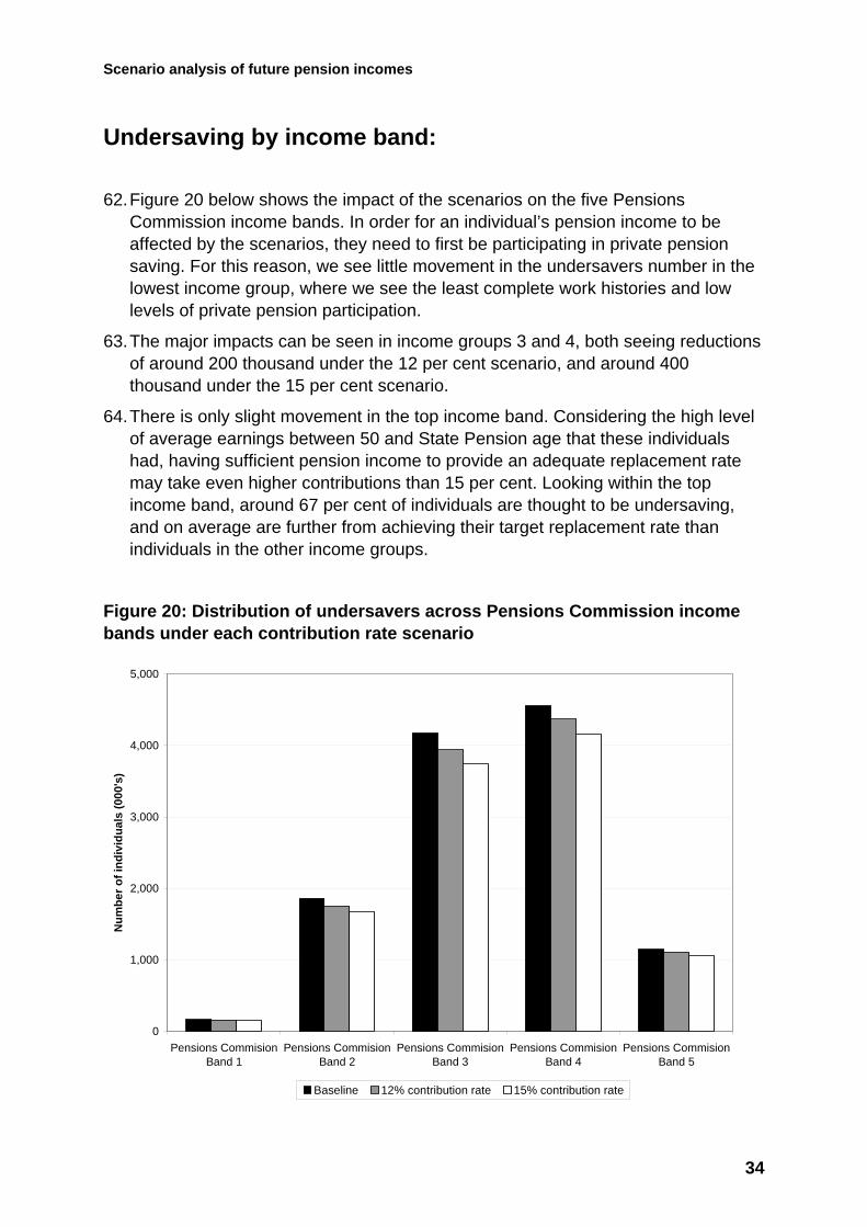
62. Figure 20 below shows the impact of the scenarios on the five Pensions Commission income bands. In order for an individual’s pension income to be affected by the scenarios, they need to first be participating in private pension saving. For this reason, we see little movement in the undersavers number in the lowest income group, where we see the least complete work histories and low levels of private pension participation.
63. The major impacts can be seen in income groups 3 and 4, both seeing reductions of around 200 thousand under the 12 per cent scenario, and around 400 thousand under the 15 per cent scenario.
64. There is only slight movement in the top income band. Considering the high level of average earnings between 50 and State Pension age that these individuals had, having sufficient pension income to provide an adequate replacement rate may take even higher contributions than 15 per cent. Looking within the top income band, around 67 per cent of individuals are thought to be undersaving, and on average are further from achieving their target replacement rate than individuals in the other income groups.
Figure 20: Distribution of undersavers across Pensions Commission income bands under each contribution rate scenario
0
1,000
2,000
3,000
4,000
5,000
Pensions CommisionBand 1
Pensions CommisionBand 2
Pensions CommisionBand 3
Pensions CommisionBand 4
Pensions CommisionBand 5
Num
ber o
f ind
ivid
uals
(000
's)
Baseline 12% contribution rate 15% contribution rate
34
Scenario analysis of future pension incomes
Undersavers by depth of undersaving:
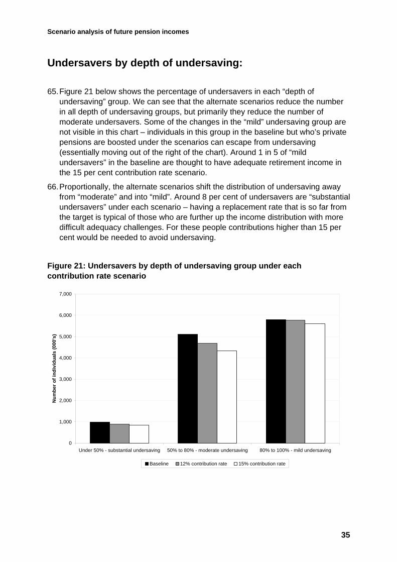
65. Figure 21 below shows the percentage of undersavers in each “depth of undersaving” group. We can see that the alternate scenarios reduce the number in all depth of undersaving groups, but primarily they reduce the number of moderate undersavers. Some of the changes in the “mild” undersaving group are not visible in this chart – individuals in this group in the baseline but who’s private pensions are boosted under the scenarios can escape from undersaving (essentially moving out of the right of the chart). Around 1 in 5 of “mild undersavers” in the baseline are thought to have adequate retirement income in the 15 per cent contribution rate scenario.
66. Proportionally, the alternate scenarios shift the distribution of undersaving away from “moderate” and into “mild”. Around 8 per cent of undersavers are “substantial undersavers” under each scenario – having a replacement rate that is so far from the target is typical of those who are further up the income distribution with more difficult adequacy challenges. For these people contributions higher than 15 per cent would be needed to avoid undersaving.
Figure 21: Undersavers by depth of undersaving group under each contribution rate scenario
0
1,000
2,000
3,000
4,000
5,000
6,000
7,000
Under 50% - substantial undersaving 50% to 80% - moderate undersaving 80% to 100% - mild undersaving
Num
ber o
f ind
ivid
uals
(000
's)
Baseline 12% contribution rate 15% contribution rate
35

Scenario analysis of future pension incomes
67. Table 11 shows the average (median) of the pension income measure used in the undersavers methodology for those people affected by the alternate contribution rate scenarios. More noticeable in the 15 per cent contribution rate scenario is the larger impact on “mild” undersavers in comparison to the “substantial” group.
• The ”mild” undersaver group has a larger composition of individuals with substantial contribution histories in the baseline. The higher contribution rate therefore has the direct impact of increasing the amount they save each year.
• “Substantial” undersavers are more likely to be individuals with broken work histories, or people with work histories but who did not contribute. The impact is understandably muted as a larger proportion of this group are not in work and not saving; so do not benefit from higher contribution rates.
Table 11: Average (median) annual pension income by depth of undersaving group under each contribution rate scenario (2014 earnings terms)
Scenario Average (median) pension income of undersavers
Among “substantial” undersavers (under 50% target achieved)
Among “moderate” undersavers (50% - 80% target achieved)
Among “mild” undersavers (80% - 100% target achieved)
Baseline (those affected by 12% scenario)
£15,800 £11,000 £14,700 £17,400
12% Contribution rate (those affected)
£16,300 £11,300 £15,200 £17,800
Baseline (those affected by 15% scenario)
£15,800 £10,800 £14,700 £17,300
15% Contribution rate (those affected)
£16,600 £11,400 £15,500 £18,200
36
Scenario analysis of future pension incomes
Cohort impacts:
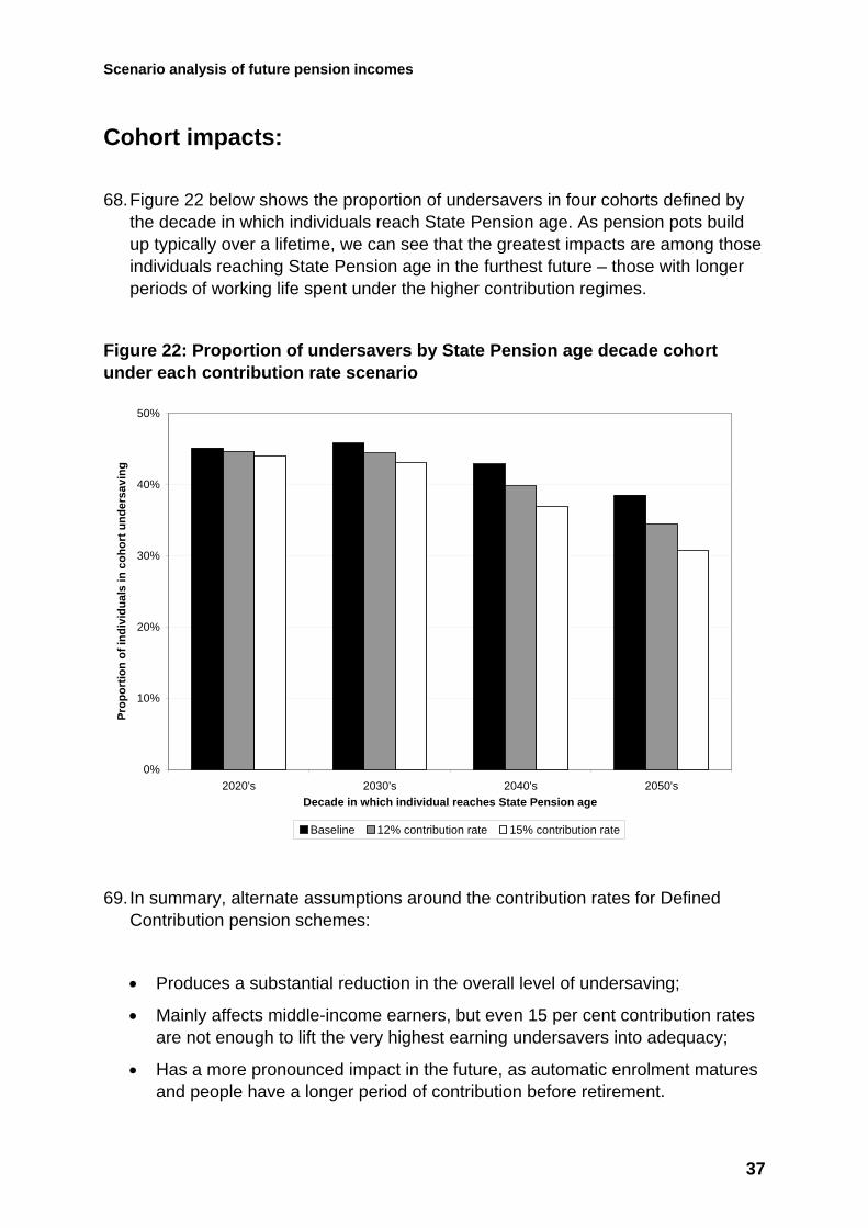
68. Figure 22 below shows the proportion of undersavers in four cohorts defined by the decade in which individuals reach State Pension age. As pension pots build up typically over a lifetime, we can see that the greatest impacts are among those individuals reaching State Pension age in the furthest future – those with longer periods of working life spent under the higher contribution regimes.
Figure 22: Proportion of undersavers by State Pension age decade cohort under each contribution rate scenario
0%
10%
20%
30%
40%
50%
2020's 2030's 2040's 2050'sDecade in which individual reaches State Pension age
Prop
ortio
n of
indi
vidu
als
in c
ohor
t und
ersa
ving
Baseline 12% contribution rate 15% contribution rate
69. In summary, alternate assumptions around the contribution rates for Defined Contribution pension schemes:
• Produces a substantial reduction in the overall level of undersaving;
• Mainly affects middle-income earners, but even 15 per cent contribution rates are not enough to lift the very highest earning undersavers into adequacy;
• Has a more pronounced impact in the future, as automatic enrolment matures and people have a longer period of contribution before retirement.
37

Scenario analysis of future pension incomes
What is the impact of up-rating the new State Pension by earnings?
Description of the scenario area:
70. In line with the Office for Budget Responsibility’s long-term assumptions, our modelling assumes that the New State pension will be indefinitely up-rated by the triple-lock mechanism which takes the highest of prices, earnings or 2.5 per cent. This is consistent with the Department’s recent publications: “Framework for the analysis of future pension income” and “The single-tier pension: a simple foundation for saving”.
71. Our “what if” looks at the alternative assumption of revaluing the new State Pension each year by the Average Earnings Index (AEI).
72. This publication focuses on the impact of policy on the adequacy of retirement income. Changing the up-rating mechanism is likely to have cost implications although these are not considered here5.
73. The impact of changing up-rating assumptions is dependent on forecasts for prices and earnings. Medium term projections are taken from the Office for Budget Responsibility’s (OBR) estimates for Budget 2014.
74. From 2019, the long term projections commence assuming growth of AEI at 4.45 per cent and growth in prices (using Consumer Prices Index) at 2 per cent. These assumptions are consistent with the Fiscal Sustainability Report 2014.
75. The new State Pension is up-rated in the baseline by the highest of AEI, CPI and 2.5 per cent up to 2018. From 2019, it is up-rated by 4.75 per cent making the assumption that overall AEI will be higher than CPI although a small adjustment upwards is made for a number of times this will not be the case.
76. For the earnings scenario, the new State Pension is up-rated by AEI from implementation in 2016.
Key direct impacts:
77. Making up-rating changes to the new State Pension primarily impacts those who retire further into the future as:
5 Assessment of the potential costs of the new State Pension under alternate starting rate and up-rating assumptions can be found in the Pensions Act 2014 Impact Assessments. https://www.gov.uk/government/publications/pensions-act-2014-impact-assessments-may-2014
38

Scenario analysis of future pension incomes
• more pensioners gain qualifying years under the new system; and
• the difference between the full value of the new State Pension up-rated by triple lock and earnings increases into the future. This is displayed in Figure 23 below.
Figure 23: Weekly full value (cash terms) of the new State Pension up-rated by triple lock and earnings
£0
£200
£400
£600
£800
£1,000
£1,200
£1,400
2016
2018
2020
2022
2024
2026
2028
2030
2032
2034
2036
2038
2040
2042
2044
2046
2048
2050
2052
2054
2056
2058
2060
Full
valu
e of
New
Sta
te p
ensi
on (c
ash
term
s)
Baseline - triple lock Average earnings index
78. By 2060, the value of the full new State Pension with triple lock up-rating is over 12 per cent higher than the earnings up-rating scenario.
39
Scenario analysis of future pension incomes
Headline changes:
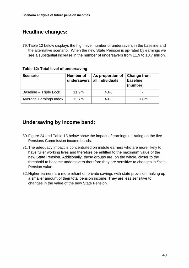
79. Table 12 below displays the high level number of undersavers in the baseline and the alternative scenario. When the new State Pension is up-rated by earnings we see a substantial increase in the number of undersavers from 11.9 to 13.7 million.
Table 12: Total level of undersaving
Scenario Number of undersavers
As proportion of all individuals
Change from baseline (number)
Baseline – Triple Lock 11.9m 43% -
Average Earnings Index 13.7m 49% +1.8m
Undersaving by income band:
80. Figure 24 and Table 13 below show the impact of earnings up-rating on the five Pensions Commission income bands.
81. The adequacy impact is concentrated on middle earners who are more likely to have fuller working lives and therefore be entitled to the maximum value of the new State Pension. Additionally, these groups are, on the whole, closer to the threshold to become undersavers therefore they are sensitive to changes in State Pension value.
82. Higher earners are more reliant on private savings with state provision making up a smaller amount of their total pension income. They are less sensitive to changes in the value of the new State Pension.
40

Scenario analysis of future pension incomes
Figure 24: Undersavers by Pensions Commission income band
0
1,000
2,000
3,000
4,000
5,000
6,000
Pensions CommissionBand 1
Pensions CommissionBand 2
Pensions CommissionBand 3
Pensions CommissionBand 4
Pensions CommissionBand 5
Num
ber o
f ind
ivid
uals
(tho
usan
ds)
Baseline - Triple lock Average Earnings Index
Table 13: Undersavers by Pensions Commission income band
Band 1 (under £12,300)
Band 2 (£12,300 to £22,700)
Band 3 (£22,700 to £32,500)
Band 4 (£32,500 to £52,000)
Band 5 (over £52,000)
Baseline – Triple Lock 0.2m 1.9m 4.2m 4.6m 1.1m
Average Earnings Index
0.2m 2.5m 4.9m 5.0m 1.2m
Undersavers by depth of undersaving:
83. Figure 25 below shows the number of undersavers broken down by “depth of undersaving” groups.
84. There is only a small impact on the total number substantially undersaving. This group is largely higher earners with less complete work histories. The cash increases that need to be made to pension income to improve adequacy, and the
41

Scenario analysis of future pension incomes
lower entitlement to State Pension from their broken work histories means that switching to up-rating by earnings has a muted effect.
85. There is a significant increase in individuals who are mild undersavers which is logical as low and middle earners who are just achieving their replacement rate are likely to join this group.
86. No individual moves down two depth of undersaving groups. Around three quarters of individuals who become moderate undersavers from mild undersaving are from middle income bands (3 and 4).
Figure 25: Undersavers by depth of undersaving group
0
1,000
2,000
3,000
4,000
5,000
6,000
7,000
Under 50% - substantial undersaving 50% to 80% - moderate undersaving 80% to 100% - mild undersaving
Num
ber o
f ind
ivid
uals
(tho
usan
ds)
Baseline - triple lock Average earnings index
87. Table 14 shows the average (median) of the pension income measure used in the undersavers methodology. Of those who will not hit their target replacement rate, up-rating the new State Pension by earnings causes a fall in annual pension income of around £800.
88. The median income among substantial undersavers does not change due to few people joining this group.
42

Scenario analysis of future pension incomes
Table 14: Average (median) annual pension income by depth of undersaving group (2014 earnings terms)
Average (median) pension income of undersavers
Among “substantial” undersavers
Among “moderate” undersavers
Among “mild” undersavers
Baseline – Triple Lock £15,300 £9,600 £14,300 £17,100
Average Earnings Index
£14,500 £9,600 £13,900 £16,300
Cohort impacts:
89. Figure 26 below shows the proportion of undersavers in four cohorts defined by the decade in which individuals reach State Pension age.
90. There is only a small difference in the percentage of undersavers retiring in the 2020s cohort. With earnings up-rating 44 per cent of those retiring during these years are undersavers where as with triple lock it is 42 per cent.
91. Of those retiring in the 2050s, around 40 per cent are undersaving with triple lock compared to around 50 per cent with earnings up-rating.
43

Scenario analysis of future pension incomes
Figure 26: Proportion of undersavers by State Pension age decade cohort
0%
10%
20%
30%
40%
50%
60%
2020's 2030's 2040's 2050's
Per
cent
age
of in
divi
dual
s un
ders
avin
g
Baseline - triple lock Average earnings index
92. In summary, up-rating the new State Pension by earnings instead of triple lock:
• causes a significant increase in the number of undersavers;
• mainly affects middle-income earners; and
• has the biggest impact on those retiring further in to the future.
44
Scenario analysis of future pension incomes
What if the full rate of the New State pension were higher?
Description of the scenario area:
93. The new State Pension will be introduced in 2016. As it is available to all eligible individuals and is given at a flat rate, irrespective of income (but dependent on the number of qualifying years a person has accrued), it is an interesting area to investigate as a “what if”.
94. The ”what if” will allow us to understand where increases to the state pension will have the most impact on undersaving, and how the Triple Lock up-rating combines with different starting rates to reduce the number of undersavers in the future.
95. The baseline scenario for the new State Pension starting rate is:
• £148.40 per week, or £7,716.80 per year in 2014 prices.
• In PenSim2 the value of the new State Pension is up rated by the long-term average Triple-Lock guarantee, which is 4.75 per cent.
96. Our “what if” looks at three alternative starting rates:
• A small increase of 70p per week, to £149.10, £7,753.20 per year;
• A starting rate of £150.10, or £7,805.20 per year; and,
• A larger increase to £154.20 per week, or £8,018.40 per year.
97. Similarly to our State Pension up-rating ”what if” we are focusing on the impact of policy on the adequacy of retirement income. Changing the starting rate of the new State Pension will have cost implications and these are not considered as part of this investigation.
45

Scenario analysis of future pension incomes
Key direct impacts:
98. As the new State Pension is a fixed amount per year, we can expect that changes to this factor will have limited impact on those with high pension incomes as the State Pension comprises a smaller proportion of their total income.
99. The triple-lock up-rating of the new State Pension will have a larger impact on higher initial starting rates. We can expect that the impact on undersaver numbers will be greater in later years for larger starting rates.
Headline changes:
100. There are around 11.9m undersavers in our baseline model. As we increase the value of the starting rate we observe a reduction in the number of undersavers. From 11.8m for a start rate of £149.10, to 11.3m for the largest starting rate we test, £154.20 per week.
Table 15: Total level of undersaving under each starting rate scenario
Scenario Number of undersavers
As proportion of all individuals
Change from baseline (number)
Baseline: Start Rate = £148.40 11.9m 43%
Start Rate = £149.10 11.8m 43% -100k
Start Rate = £150.10 11.7m 42% -200k
Start Rate = £154.20 11.3m 41% -650k
101. The relationship between the starting rate and number of undersavers is strongly linear between our Baseline and the highest start rate, £154.20. Each increase of £1 in the starting rate equates to around 111,000 fewer undersavers up to the year 2059.
46

Scenario analysis of future pension incomes
Undersaving by income band:
102. Table 16 shows the impacts of the different starting rate scenarios on the number of undersavers in our five income bands. As we would expect, increases to the State Pension income consistently reduce the number of undersavers in the system.
Table 16: Number of undersavers in each Pensions Commission income band under each starting rate scenario
Starting Rate scenario
Band 1
(under £12,300)
Band 2 (£12,300 to £22,700)
Band 3
(£22,700 to £32,500)
Band 4
(£32,500 to £52,000)
Band 5
(over £52,000)
Baseline: Start Rate = £148.40 0.2m 1.9m 4.2m 4.6m 1.1m
Start Rate = £149.10 0.2m 1.8m 4.1m 4.5m 1.1m
Start Rate = £150.10 0.2m 1.8m 4.1m 4.5m 1.1m
Start Rate = £154.20 0.1m 1.7m 3.9m 4.4m 1.1m
103. Figure 27 shows us the impact that changing the starting rate has on undersavers across the five income bands, compared to the baseline scenario.
104. The increase in the starting rate has a more potent affect on the number of undersavers in the middle income groups. With a £154.20 starting rate there are 250,000 fewer undersavers in the ‘Middle’ income group than we see in the baseline scenario, compared to only around 20,000 in the lowest and highest income groups.
47

Scenario analysis of future pension incomes
Figure 27: The number of undersavers by income band under each starting rate scenario
0
500
1000
1500
2000
2500
3000
3500
4000
4500
5000
PensionCommission Band 1
PensionCommission Band 2
PensionCommission Band 3
PensionCommission Band 4
PensionCommission Band 5
Num
ber o
f und
ersa
vers
(tho
usan
ds)
Baseline £149.10 scenario £150.10 scenario £154.20 scenario
105. The focus of the impact on the middle income groups stems from two factors:
• These are the largest groups by population; and,
• These groups have the peak of their undersaving depth distribution close to the “undersaver-adequate threshold”, making it easy to achieve threshold gains.
106. The lowest income group has most individuals well above the “adequate threshold”, and the highest income band has its peak in the “moderate undersaver” region. This is in comparison to the middle income group, which has the most individuals just below the “undersaver-adequate threshold”, thereby making it very easy to “push” many individuals over into adequacy.
Undersavers by depth of undersaving:
107. Figure 28 shows the number of undersavers in the undersaver depth bands. The largest impact is seen in the “moderate undersaver” group.
108. We observe little impact in the “substantial undersaver” group. As this depth band is dominated by those on higher incomes it is understandable that relatively small increases to their pension income will not cause notable movement for
48

Scenario analysis of future pension incomes
these individuals who require larger cash increases in pension income to improve their adequacy. Individuals in this depth band also have less complete work histories which in turn leads to reduced eligibility for State Pension, further muting the impact of this “what if”.
109. Likewise, we see a fairly stable population in the “mild undersaver” group. The stability for this group is explained by the similar in- and out-flow rates of individuals from the “moderate” and to the “adequate” groups. These flows are similar because the numbers of individuals that are able to step-up and out of their baseline group are similar.
Figure 28: The number of undersavers in each depth band under each starting rate scenario
0
1000
2000
3000
4000
5000
6000
7000
Under 50% - substantialundersaving
50% to 80% - moderateundersaving
80% to 100% - mild undersaving
Num
ber o
f und
ersa
vers
(tho
usan
ds)
Baseline £149.10 scenario £150.10 scenario £154.20 scenario
110. We see lots of movement out of the “moderate” group because of the difference between the number of individuals that move into and out of this group. The “substantial” undersaver group is quite immobile, while those in the higher end of the “moderate” group are more easily able to improve their undersaving position through an increase to their state pension.
111. These factors combine to produce a positive impact on the situation of undersavers in the pension system. These increases to the new State Pension starting rate can lead to many individuals becoming adequate, as well as many more improving their pension income and therefore position as an undersaver.
49

Scenario analysis of future pension incomes
Cohort impacts:
112. We can expect an increase in the starting rate to have a positive impact on the number of undersavers in the future because of the increase from the triple-lock guarantee. The higher the state pension is initially, the more rapidly it will grow and help reduce undersaver numbers.
Figure 29: The proportion of undersavers by the decade they reach State Pension age under each starting rate scenario
0%
5%
10%
15%
20%
25%
30%
35%
40%
45%
50%
2020's 2030's 2040's 2050's
Perc
enta
ge o
f ind
ivid
uals
und
ersa
ving
Baseline £149.10 scenario £150.10 scenario £154.20 scenario
113. We can see that this is the case in Figure 29, where starting rates above the Baseline give improvements to the number of undersavers compared to the Baseline for all decades.
114. In summary, the new State Pension provides the basis of the pension system. Increasing the starting rate would reduce the number of undersavers across all income groups, particularly those in the middle income groups.
50

Scenario analysis of future pension incomes
Annex A: Selecting the Fuller Working Lives cohort for the employment “what if” analysis The following diagram explains how we select the Fuller Working Lives cohort from the analysis, on which the employment “what if” analysis centres:
27.5m have all the required information across the three scenarios; baseline, modest and substantial. (Because they are each 'full runs' - some people appear in the baseline population but not in the uplift populations)
24.1m experience no decline in years worked between 50-SPa in either of the employment scenarios:
• 8.4m see no change in either the modest or substantial uplifts.
• 5.6m see an increase in one of the scenarios but no change in the other - inconsistent impacts.
• 10.1m consistently experience an increase in years worked in both alternative scenarios - the group we focus on.
3.4m experience a decline in the number of years worked between 50-SPa relative to the baseline in either one or both of the uplift scenarios:
• Over 85% of this group see a fall in one scenario but not in the other - not ideal to focus on these people with inconsistent impacts.
• Leaving only 460k individuals who consistently see a fall from their baseline years worked in both uplift scenarios.
27.8m baseline population above the GC threshold
51

Scenario analysis of future pension incomes
Annex B: In-depth focus on contribution rates to Defined Contribution pension schemes
This chapter will take a more in-depth look at the contribution rate ”what if”. It will focus on:
• The cohort impact in more detail through analysing the depth of undersaving and pattern of undersaving across time.
• The link between higher contribution rates and the numbers facing inadequate retirement incomes.
• A ‘mixed’ model in which contribution rates are staggered with Pensions Commission Income bands.
Cohort impact in more detail:
115. The earlier chapter on contribution rates showed how, over time, the difference in the proportion of undersavers between the scenarios widened – for those reaching State Pension age in the 2050’s, 31 per cent are projected to be inadequate in the 15 per cent contribution rate model compared to 39 per cent in the baseline. For the 2020’s cohort, the proportions in the two models differ by only 1 percentage point.
116. Another way to look at this is to group the adequacy population by their age in 2014. Figure 30 below shows how the younger cohorts (those retiring later) experience a greater improvement under higher contribution rates as they spend a larger proportion of their working lives under automatic enrolment.
52
Scenario analysis of future pension incomes
Figure 30: Proportion of each age cohort who are undersavers under each contribution rate scenario (Age in 2014)
0%
10%
20%
30%
40%
50%
30 or younger 31 - 40 41 - 50 51 - 60 60+
Prop
ortio
n of
indi
vidu
als
Baseline 12% contribution rate 15% contribution rate
117. In later cohorts therefore, the higher contribution rates have an increasing impact on reducing headline undersavers. For those who remain undersaving, we can see if, over time, the depth and pattern of undersaving changes.
Undersaving by depth over time:
118. Table 17 explores how the composition of undersavers changes over time. For undersavers retiring in the 2050’s, approximately 1 in 20 are “substantial” undersavers (those achieving a replacement rate less than half of their target) in both the baseline and 15 per cent contributions model. The static proportion is understandable given this group is over-represented by people with higher incomes during working life, but who have broken work histories. Therefore they are largely unaffected by higher contribution rates.
119. Noticeable between the two models is the shift in proportion from “moderate” to “mild”. Of undersavers retiring in the 2050’s, 64 per cent are “mild” in the 15 per cent contribution rate model compared to 57 per cent in the baseline – Not only does the higher contribution rate reduce the number facing inadequate retirement incomes but, of those who remain undersaving, a greater proportion are achieving over 80 per cent of their target.
53

Scenario analysis of future pension incomes
Table 17: Depth of undersaving over time, baseline and 15 per cent contribution rate scenarios
Decade SPA cohort
Number of undersavers
Proportion "substantial"
Proportion "moderate"
Proportion "mild"
Baseline - 8% contribution rate
2020's 2.7m 13% 46% 41%
2030's 3.4m 8% 45% 47%
2040's 2.5m 5% 41% 54%
2050's 2.5m 5% 38% 57%
15% contribution rate
2020's 2.6m 12% 46% 41%
2030's 3.2m 7% 42% 51%
2040's 2.1m 4% 37% 58%
2050's 2.0m 4% 32% 64%
Undersaving by income band over time:
120. Figure 20 showed how higher contribution rates have a greater impact on the middle Pensions Commission income bands. Figure 31 below shows that this is consistent over time. Whilst the scale of impact is larger in later cohorts, it is still the case that individuals in income bands 2, 3 and 4 see the majority of replacement rate improvements.
54

Scenario analysis of future pension incomes
Figure 31: Individuals made adequate in the 15 per cent contribution rate model grouped by Pensions Commission income band and State Pension age decade cohort.
0
40
80
120
160
200
240
2020's 2030's 2040's 2050's
Indi
vidu
als
mad
e ad
equa
te (t
hous
ands
)
PC Band 1 PC Band 2 PC Band 3 PC Band 4 PC Band 5
Note: The 12 per cent contribution rate model shows the same pattern.
121. As a consequence, Table 18 shows how higher contribution rates do little to change the pattern of undersaving relative to the baseline.
• In each scenario approximately 1-2 per cent of total undersavers come from the lowest income band and around 10 per cent from the highest. There is a slight proportional shift in undersaver prevalence over time from Pensions Commission band 2 towards band 4, but this is seen in both the baseline and alternate scenarios.
55

Scenario analysis of future pension incomes
Table 18: Pattern of undersaving over time
Decade SPA cohort
Number of undersavers
% PC Band 1 (Under £12,300)
% PC Band 2 (£12,300 to £22,700)
% PC Band 3 (£22,700 to £32,500)
% PC Band 4 (£32,500 to £52,000)
% PC Band 5 (Over £52,000)
Baseline - 8% contribution rate
2020's 2.7m 2% 18% 35% 34% 11%
2030's 3.4m 1% 16% 35% 38% 10%
2040's 2.5m 1% 14% 35% 42% 9%
2050's 2.5m 1% 13% 36% 40% 10%
15% contribution rate
2020's 2.6m 2% 18% 35% 35% 11%
2030's 3.2m 1% 16% 34% 38% 10%
2040's 2.1m 1% 13% 34% 43% 9%
2050's 2.0m 1% 13% 35% 41% 10%
Contribution rates and headline undersavers:
122. Increases in contributions mean replacement rate improvements for more people. For those with DC contribution histories, Figure 32 shows the average contribution rate in the baseline scenario.
123. As the contribution rate rises (and therefore moves to the right on the x-axis), the numbers impacted grows. For example, at 12 per cent all those to the left of the dotted line are affected.
124. Increasing contributions from 8 to 12 per cent would impact around two-fifths of the adequacy population. Moving from 8 to 15 per cent would impact over three-fifths of the population.
56

Scenario analysis of future pension incomes
Figure 32: Average occupational DC contribution rates amongst those with DC contribution histories
0%
10%
20%
30%
LESS THEN 2%
BETWEEN 2% AND 4%
BETWEEN 4% AND 6%
BETWEEN 6% AND 8%
BETWEEN 8% AND 10
%
BETWEEN 10% AND 12
%
BETWEEN 12% AND 15
%
OVER 15%
Average contribution rate
Pro
porti
on o
f ind
ivid
uals
125. Figure 33 below shows how this growing impact of higher contribution rates
translates into headline undersaver reductions.
57

Scenario analysis of future pension incomes
Figure 33: Headline undersaver numbers under different combined contribution rates
8,000
9,000
10,000
11,000
12,000
13,000
Baseline - 8% 10% 12% 15% 18% 20%
Contribution Rate
Num
ber o
f ind
ivid
uals
(tho
usan
ds)
Mixed contribution rates The three initial scenarios (8 (baseline), 12 and 15 per cent) model variations in the contribution rates for Defined Contribution pension schemes. In each case, the rate universally applies to all members. We have seen however that individuals at the lower end of the earnings distribution are well provided for by the State Pension, and it is higher earners who can gain more by contributing at a higher rate. Indeed, higher contribution rates for lower earners could be detrimental, diverting day-to-day living funds into pension saving. In this “mixed” contribution analysis we look at what would happen if the contribution rates varied across Pensions Commission income bands.
58
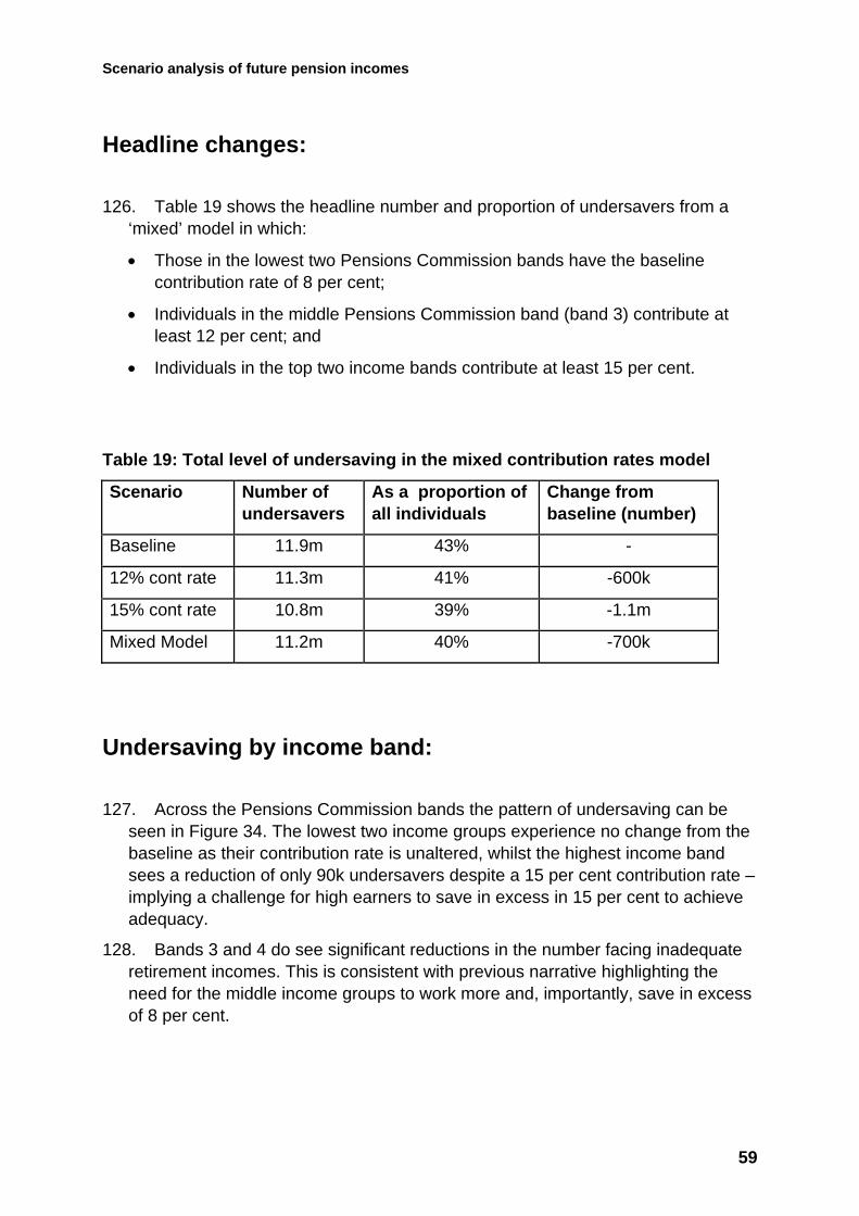
Scenario analysis of future pension incomes
Headline changes:
126. Table 19 shows the headline number and proportion of undersavers from a ‘mixed’ model in which:
• Those in the lowest two Pensions Commission bands have the baseline contribution rate of 8 per cent;
• Individuals in the middle Pensions Commission band (band 3) contribute at least 12 per cent; and
• Individuals in the top two income bands contribute at least 15 per cent.
Table 19: Total level of undersaving in the mixed contribution rates model
Scenario Number of undersavers
As a proportion of all individuals
Change from baseline (number)
Baseline 11.9m 43% -
12% cont rate 11.3m 41% -600k
15% cont rate 10.8m 39% -1.1m
Mixed Model 11.2m 40% -700k
Undersaving by income band:
127. Across the Pensions Commission bands the pattern of undersaving can be seen in Figure 34. The lowest two income groups experience no change from the baseline as their contribution rate is unaltered, whilst the highest income band sees a reduction of only 90k undersavers despite a 15 per cent contribution rate – implying a challenge for high earners to save in excess in 15 per cent to achieve adequacy.
128. Bands 3 and 4 do see significant reductions in the number facing inadequate retirement incomes. This is consistent with previous narrative highlighting the need for the middle income groups to work more and, importantly, save in excess of 8 per cent.
59

Scenario analysis of future pension incomes
Figure 34: Undersavers by Pensions Commission income band in the mixed contribution rate model
0
1,000
2,000
3,000
4,000
5,000
PensionsCommission Band 1
PensionsCommission Band 2
PensionsCommission Band 3
PensionsCommission Band 4
PensionsCommission Band 5
Num
ber o
f ind
ivid
uals
(tho
usan
ds)
Baseline 8% Mixed Model
Undersavers by depth of undersaving:
129. Figure 35 breaks the undersaver number down by “depth of undersaving” groups with ‘depth’ referring to how far the individual is from achieving their target replacement rate.
130. Noticeable is that the ‘mixed’ model has the greatest impact on the “moderate” undersavers. This is the same pattern seen in both the 12 and 15 per cent scenarios.
131. “Substantial” undersavers are disproportionately represented by higher earners with broken work histories; therefore higher contribution rates do not get to the crux of the issue.
132. The “moderate” undersaver group is largely populated by middle income individuals – individuals for whom the adequacy challenge revolves around working for more years and contributing at a slightly higher rate. Higher contribution rates, be it 12 or 15 per cent in our mixed model, therefore directly helps to boost adequacy.
60
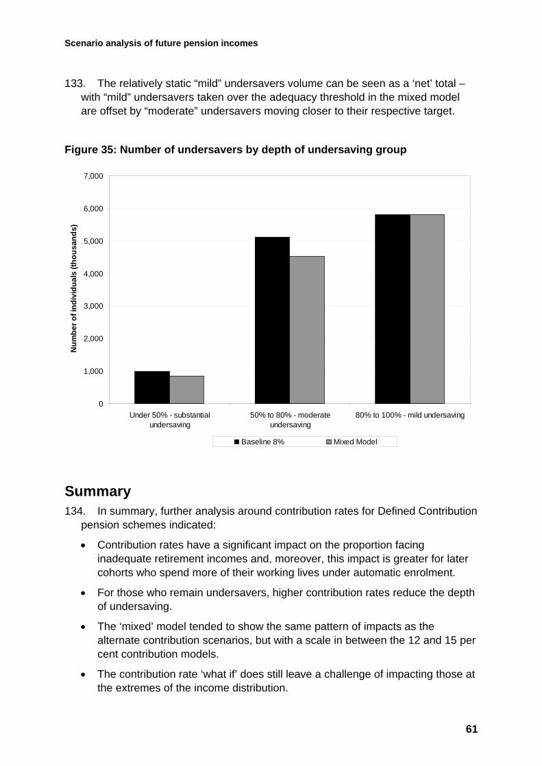
Scenario analysis of future pension incomes
61
133. The relatively static “mild” undersavers volume can be seen as a ‘net’ total – with “mild” undersavers taken over the adequacy threshold in the mixed model are offset by “moderate” undersavers moving closer to their respective target.
Figure 35: Number of undersavers by depth of undersaving group
0
1,000
2,000
3,000
4,000
5,000
6,000
7,000
Under 50% - substantialundersaving
50% to 80% - moderateundersaving
80% to 100% - mild undersaving
Num
ber o
f ind
ivid
uals
(tho
usan
ds)
Baseline 8% Mixed Model
Summary 134. In summary, further analysis around contribution rates for Defined Contribution
pension schemes indicated:
• Contribution rates have a significant impact on the proportion facing inadequate retirement incomes and, moreover, this impact is greater for later cohorts who spend more of their working lives under automatic enrolment.
• For those who remain undersavers, higher contribution rates reduce the depth of undersaving.
• The ‘mixed’ model tended to show the same pattern of impacts as the alternate contribution scenarios, but with a scale in between the 12 and 15 per cent contribution models.
• The contribution rate ‘what if’ does still leave a challenge of impacting those at the extremes of the income distribution.

Scenario analysis of future pension incomes
Annex C: In-depth focus on up-rating of the new State Pension
This chapter will look in more detail at how retirement income adequacy is affected by up-rating the new State Pension by growth in average earnings, focussing on:
• how dependent individuals are on the State Pension;
• which income groups are affected by changes in up-rating; and
• the dynamic impacts on the depth of undersaving.
Headline undersavers increase by 1.8 million from 11.9 to 13.7 mainly due to the fact that the change has an impact on the majority of individuals in our measure. It has a marked impact across the income distribution although no single Pensions Commission income band is severely affected in isolation.
Our findings are supported by the Pensions Policy Institute’s recent publication on retirement income adequacy which found that increasing the new State Pension by the highest of earnings, prices and 2.5 per cent is a significant factor in preventing undersaving6.
How reliant are individuals on their State Pension income?
135. Individuals who are heavily reliant on the State Pension are adversely affected by lowering its value.
136. The new State Pension, set above the basic level of means-tested support, will provide a foundation for saving for moderate to high earners who are more likely to have private pension provision. In addition, higher earners are more likely to contribute at a higher rate to Defined Contribution (DC) schemes and have fuller work histories.
137. For lower earners (those in Pensions Commission band 1) the full new State Pension amount is likely to ensure adequacy.
138. In Figure 36 we look at the State Pension component of our measure of pension age income used in the replacement rate calculations (the average income over all years spent in retirement equivalised for household size). The chart suggests that
6 PPI, What level of pension contribution is needed to obtain an adequate retirement income?
62

Scenario analysis of future pension incomes
on average, between now and 2060, the majority of pension income for low to middle earners is provided by the State Pension. In contrast, individuals in the two highest income bands have, on average, around half their income provided by the State.
Figure 36: State Pension as a proportion of total pension income by Pensions Commission income band
78%
71%
63%
55%
45%
78%
70%
62%
53%
43%
0%
10%
20%
30%
40%
50%
60%
70%
80%
90%
Pensions CommissionBand 1
Pensions CommissionBand 2
Pensions CommissionBand 3
Pensions CommissionBand 4
Pensions CommissionBand 5
Per
cent
age
of to
tal p
ensi
on in
com
e
Baseline - triple lock Average earnings index
139. Across all income bands, income from the State as a proportion of total pension income falls by around 1 percentage point when switching to earnings up-rating. In Figure 36 there is only a small difference as we are looking from now until 2060.
140. The impact of up-rating the new State Pension by earnings on adequacy will become more obvious from the 2040s onwards as the difference, in comparison to up-rating by triple lock, increases.
141. In Figure 37 we look at the State Pension component of our measure of pension age income split by the decade in which individuals reach State Pension age. For the 2020’s cohort the median State Pension component falls by around £500 when up-rated by earnings. By 2060, there is a difference in of around £1,600.
63

Scenario analysis of future pension incomes
Figure 37: Median annual State Pension income by SPa decade cohort (2014 earnings terms)
£0
£2,000
£4,000
£6,000
£8,000
£10,000
£12,000
£14,000
2020's 2030's 2040's 2050's
Ann
ual S
tate
pen
sion
inco
me
Baseline - triple lock Average earnings index
142. The larger difference in State Pension value in the future means that those who are 30 and younger in 2014 will be at an increased risk of undersaving. Figure 38 shows around half of this age cohort are undersaving in retirement when up-rating the new State Pension by earnings.
64
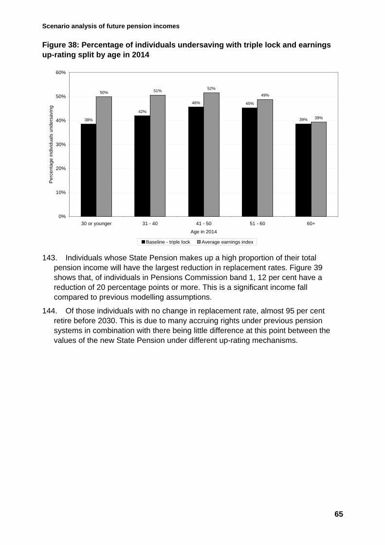
Scenario analysis of future pension incomes
Figure 38: Percentage of individuals undersaving with triple lock and earnings up-rating split by age in 2014
38%
42%
46% 45%
39%
50% 51% 52%49%
39%
0%
10%
20%
30%
40%
50%
60%
30 or younger 31 - 40 41 - 50 51 - 60 60+
Age in 2014
Per
cent
age
indi
vidu
als
unde
rsav
ing
Baseline - triple lock Average earnings index 143. Individuals whose State Pension makes up a high proportion of their total
pension income will have the largest reduction in replacement rates. Figure 39 shows that, of individuals in Pensions Commission band 1, 12 per cent have a reduction of 20 percentage points or more. This is a significant income fall compared to previous modelling assumptions.
144. Of those individuals with no change in replacement rate, almost 95 per cent retire before 2030. This is due to many accruing rights under previous pension systems in combination with there being little difference at this point between the values of the new State Pension under different up-rating mechanisms.
65

Scenario analysis of future pension incomes
Figure 39: Reduction in replacement rate when up-rating the new State Pension by earnings split by Pensions Commission income band
0%
10%
20%
30%
40%
50%
60%
70%
80%
90%
100%
Pensions CommissionBand 1
Pensions CommissionBand 2
Pensions CommissionBand 3
Pensions CommissionBand 4
Pensions CommissionBand 5
Perc
enta
ge o
f ind
ivid
uals
in g
roup
No difference -10pp -20pp Over 20pp
145. Up-rating by earnings has an impact across the income distribution. Of individuals in Pensions Commission band 5, around 90 per cent will have a reduction in their replacement rate of up to 10 percentage points although the actual reduction is much lower with a median value of 2 percentage points.
146. Although many individuals in Pensions Commission band 1 have a substantial fall in their replacement rate, with the median decrease being 13 percentage points, there is little change in the overall number of undersavers in this group. This is due to the majority of individuals having good adequacy outcomes.
147. Over 60 per cent of those in Pensions Commission band 1 obtain over 150 per cent of their target replacement rate. Up-rating the new State Pension by earnings does not cause a large number of these individuals to be classed as having inadequate retirement income.
148. However, those who will rely heavily on the new State Pension will have a drop in their retirement income when comparing the two scenarios. An individual born in 2000, earning £12,300 (Pensions Commission band 1) in constant terms working from age 25 to 65 who reaches SPa in 2068 will have £26 a week less State Pension income on average in 2014 earnings terms.
149. This individual is also enrolled into a workplace pension contributing at the minimum level which is used to buy a level annuity at retirement and provides a portion of their total pension income.
150. Despite the fall in income they remain adequate with a 14 percentage point decrease in actual replacement rate from 105 per cent to 91 per cent.
66

Scenario analysis of future pension incomes
Table 20: Adequate low earner with full working history
Average weekly State Pension
Total State Pension
Actual replacement rate
Baseline – Triple Lock £167 £243,000 105%
Average Earnings Index £141 £176,400 91%
Difference -£26 -£66,600 -14pp
151. The baseline distribution of adequacy, shown in Figure 40, shows why the lowest income band is not significantly affected in terms of the headline undersaver number. There is, however, a shift towards the left in Figure 41 (earnings up-rating) as many individuals move closer to their target replacement rate.
152. The key issue in reducing undersaving in band 1 is ensuring individuals build the 35 qualifying years needed for the full new State Pension. Increasing the generosity of up-rating or value will have little impact on adequacy outcomes as individuals in this group are more likely to have broken work histories.
Figure 40: The distribution of undersaver depth in Pensions Commission band 1 with triple lock up-rating
0
50
100
150
200
250
0 - 0
.1
0.1
- 0.2
0.2
- 0.3
0.3
- 0.4
0.4
- 0.5
0.5
- 0.6
0.6
- 0.7
0.7
- 0.8
0.8
- 0.9
0.9
- 1
1 - 1
.1
1.1
- 1.2
1.2
- 1.3
1.3
- 1.4
1.4
- 1.5
1.5
- 1.6
1.6
- 1.7
1.7
- 1.8
1.8
- 1.9
1.9
- 2
2 - 2
.1
2.1
- 2.2
2.2
- 2.3
2.3
- 2.4
2.4
- 2.5
2.5
- 2.6
2.6
- 2.7
2.7
- 2.8
2.8
- 2.9
2.9
- 3
Mor
e th
an 3
Depth
Num
ber o
f und
ersa
vers
(tho
usan
ds)
Substantial undersavers Moderate undersavers Mild undersavers Adequate savers
67

Scenario analysis of future pension incomes
Figure 41: The distribution of undersaver depth in Pensions Commission band 1 with earnings up-rating
0
50
100
150
200
2500
- 0.1
0.1
- 0.2
0.2
- 0.3
0.3
- 0.4
0.4
- 0.5
0.5
- 0.6
0.6
- 0.7
0.7
- 0.8
0.8
- 0.9
0.9
- 1
1 - 1
.1
1.1
- 1.2
1.2
- 1.3
1.3
- 1.4
1.4
- 1.5
1.5
- 1.6
1.6
- 1.7
1.7
- 1.8
1.8
- 1.9
1.9
- 2
2 - 2
.1
2.1
- 2.2
2.2
- 2.3
2.3
- 2.4
2.4
- 2.5
2.5
- 2.6
2.6
- 2.7
2.7
- 2.8
2.8
- 2.9
2.9
- 3
Mor
e th
an 3
Depth
Num
ber o
f und
ersa
vers
(tho
usan
ds)
Substantial undersavers Moderate undersavers Mild undersavers Adequate savers
153. Individuals in Pensions Commission band 3 are, overall, not as adequate in retirement. In addition, they still rely on the State pension to provide a significant amount of their retirement income. This means the removal of triple lock up-rating has a marked impact on adequacy for individuals in this income band. The situation is similar in the other Pensions Commission income bands.
68

Scenario analysis of future pension incomes
Figure 42: The distribution of undersaver depth in Pensions Commission band 3 with triple lock up-rating
0
200
400
600
800
1,000
1,200
1,4000
- 0.1
0.1
- 0.2
0.2
- 0.3
0.3
- 0.4
0.4
- 0.5
0.5
- 0.6
0.6
- 0.7
0.7
- 0.8
0.8
- 0.9
0.9
- 1
1 - 1
.1
1.1
- 1.2
1.2
- 1.3
1.3
- 1.4
1.4
- 1.5
1.5
- 1.6
1.6
- 1.7
1.7
- 1.8
1.8
- 1.9
1.9
- 2
2 - 2
.1
2.1
- 2.2
2.2
- 2.3
2.3
- 2.4
2.4
- 2.5
2.5
- 2.6
2.6
- 2.7
2.7
- 2.8
2.8
- 2.9
2.9
- 3
Mor
e th
an 3
Depth
Num
ber o
f ind
ivid
uals
(tho
usan
ds)
Substantial undersavers Moderate undersavers Mild undersavers Adequate savers Figure 43: The distribution of undersaver depth in Pensions Commission band 3 with earnings up-rating
0
200
400
600
800
1,000
1,200
1,400
0 - 0
.1
0.1
- 0.2
0.2
- 0.3
0.3
- 0.4
0.4
- 0.5
0.5
- 0.6
0.6
- 0.7
0.7
- 0.8
0.8
- 0.9
0.9
- 1
1 - 1
.1
1.1
- 1.2
1.2
- 1.3
1.3
- 1.4
1.4
- 1.5
1.5
- 1.6
1.6
- 1.7
1.7
- 1.8
1.8
- 1.9
1.9
- 2
2 - 2
.1
2.1
- 2.2
2.2
- 2.3
2.3
- 2.4
2.4
- 2.5
2.5
- 2.6
2.6
- 2.7
2.7
- 2.8
2.8
- 2.9
2.9
- 3
Mor
e th
an 3
Depth
Num
ber o
f ind
ivid
uals
(tho
usan
ds)
Substantial undersavers Moderate undersavers Mild undersavers Adequate savers
69

Scenario analysis of future pension incomes
Where do the 1.8 million new undersavers come from?
154. As stated in the first part of this chapter, the 1.8 million new undersavers are not primarily located at the bottom of the income distribution as may be inferred when looking at reliance on State income. This is due the group’s good adequacy outcomes.
155. Very few of the new undersavers are from Pensions Commission band 5, as individuals with higher earnings before State Pension age require increased private pension income and other savings to maintain or attain adequacy – the State pension is of less importance for higher earners.
156. Figure 44 shows that around 94 per cent of the new undersavers (around 1.7 million of the 1.8 million) come from Pensions Commission bands 2, 3 and 4.
Figure 44: Proportion of total new undersavers split by Pensions Commission income bands
0%
5%
10%
15%
20%
25%
30%
35%
40%
Pensions CommissionBand 1
Pensions CommissionBand 2
Pensions CommissionBand 3
Pensions CommissionBand 4
Pensions CommissionBand 5
Perc
enta
ge o
f new
und
ersa
vers
157. In terms of undersaving depth, no individual moves down more than one
undersaving group.
158. All individuals who were adequate in the baseline and become undersavers are classed as ‘mild’. Figure 45 shows there are 1.5 million new ‘moderate’ undersavers who move from being classed as ‘mildly’ undersaving. A much smaller group of individuals (around 300 thousand) move to ‘substantial’ undersaving.
70
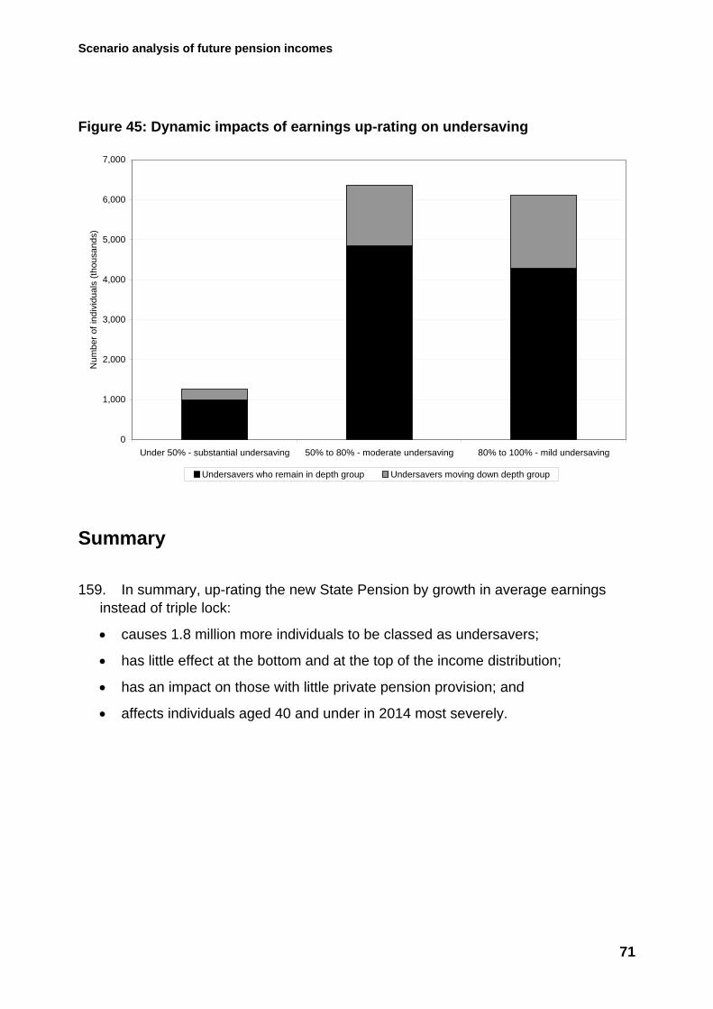
Scenario analysis of future pension incomes
Figure 45: Dynamic impacts of earnings up-rating on undersaving
0
1,000
2,000
3,000
4,000
5,000
6,000
7,000
Under 50% - substantial undersaving 50% to 80% - moderate undersaving 80% to 100% - mild undersaving
Num
ber o
f ind
ivid
uals
(tho
usan
ds)
Undersavers who remain in depth group Undersavers moving down depth group
Summary
159. In summary, up-rating the new State Pension by growth in average earnings instead of triple lock:
• causes 1.8 million more individuals to be classed as undersavers;
• has little effect at the bottom and at the top of the income distribution;
• has an impact on those with little private pension provision; and
• affects individuals aged 40 and under in 2014 most severely.
71

Scenario analysis of future pension incomes
Annex D (technical): Methodology and models used to analyse future retirement incomes Introduction This annex describes the methodology used to estimate the number of people facing inadequate retirement incomes (or ‘undersavers’). It includes the main assumptions used, the methodological choices, and a brief description of the modelling tools.
DWP Approach 160. The analysis used in this document assessed the adequacy of retirement
incomes by modelling replacement rates for simulated individuals. This allows the assessment of policy changes that will have impacts several decades in the future.
161. Replacement rates measure income in retirement as a percentage of income in work.
162. In the approach used, pre-retirement income is calculated as the average of positive earnings from age 50 until State Pension age. Key points about the definition are:
• Income is put in constant earnings terms before averaging over 50-State Pension age.
• Income is gross of tax, and of pension contributions.
• Only income from earnings is included – income from benefits, tax credits, and pensions received before State Pension age are excluded. The methodology is effectively looking at whether pension income will replace earnings.
• Only years with positive earnings are included. So someone who stops work at 55 will have the same average pre-retirement income as someone earning the same amount who continues to work up to State Pension age.
• Individuals who have no positive years of earnings between 50 and State Pension age are excluded from the analysis.
• Individuals whose average 50 to State Pension age income is below Guarantee Credit level are also excluded from the analysis – these individuals see their in-work income replaced by Pension Credit.
163. The exclusions detailed in the previous point mean that our analysis is concentrated on a population of 27.8 million people.7
7 When in our analysis we conclude that with ‘the proportion of undersavers in the baseline is around 43 per cent’, we are comparing the number of inadequate savers to this figure of 27.8 million people. This number is not equal to the total number of people aged 22 to State Pension age, the number of people in
72

Scenario analysis of future pension incomes
164. Retirement income is the income from State Pension age onwards averaged over the whole of retirement. Key points include:
• Income is in constant price terms before averaging over whole of retirement;
• Income is gross of tax;
• Income includes state and private pension income;
• Income from means tested benefits such as Pension Credit and disability benefits is excluded (although see the below section on Housing Adjustment on housing benefit);
• While financial wealth is not modelled directly, an amount is imputed and then annuitised based on Wealth and Assets Survey data;
• Only retirement income received after State Pension age is considered for the analysis.
165. For couples:
• Average pre-retirement income is calculated separately for both members, summed, then equivalised; and
• Retirement income is equivalised on a year-by-year basis, and then averaged across retirement for the members of the couple separately. This means that the members of a couple can have different replacement rates as they have different lengths of retirement.
166. The individual’s replacement rate is then compared to a benchmark to determine whether it is adequate. The benchmarks from the 2004 Pensions Commission report are used, with the income thresholds which they apply to adjusted for earnings growth. The Pensions Commission benchmarks were based on pre and post retirement income patterns, together with survey evidence of people’s expected and desired retirement income.
employment, or the workforce. The main differences are that the 27.8 million includes people currently out of work, and it excludes immigrants and people with average earnings below the Guaranteed Credit level (particularly those with no positive earnings) between 50 and State Pension age.
73

Scenario analysis of future pension incomes
Income equivalisation is a technique that recognises these economies of scale, and adjusts a couple’s income accordingly. For example, in the analysis without housing costs, each individual in a couple is assigned an income equal to 67 per cent of the whole couple’s income. When housing costs are subtracted, each individual in a couple is assigned an income equal to 58 per cent of the whole couple’s income.
In both cases, the total income assigned to the couple exceeds 100 per cent of the actual nominal income, reflecting the fact that when in a couple, each pound ‘goes further’ due to economies of scale.
Income equivalisation
When two adults live together in a couple, they usually benefit from economies of scale in their normal living costs. For example, it is expected that two adults will pay a rent or mortgage that is less than twice as much what each of them would pay if living separately. The same applies to other normal living costs (transport, utilities, etc).
Model used 167. The analysis used in this publication uses one key tool:
• Pensim2: a dynamic micro-simulation model based on a sample of synthetic individuals, reflecting the characteristics of the British population. It produces results which describe the population as a whole or subgroups, including overall numbers facing inadequate incomes.
168. A key issue is that this model does not reflect behavioural impacts of policy changes; for example, it does not reflect simplicity of the new State Pension increasing levels of saving. It is also limited in the interactions between different forms of saving that are modelled; for example, labour market and savings behaviour of couples is not interrelated, and the model does not reflect interaction between home ownership, pension saving and other financial saving.
Pensim2 169. Pensim2 starts from a set of base data representative of the GB household
population in 2006. This includes detailed information on the characteristics of individuals and their employment and pension histories to date. For each subsequent year, for each individual, sets of equations are used to model the probability of certain events occurring based on estimates from current data. The calculated probabilities are then used within the model to determine what happens to each individual in a given year up to 2100.
170. The individual labour market and pension histories generated by the model are used to calculate estimates of pensioner incomes in each year of the simulation.
74
Scenario analysis of future pension incomes
171. This analysis has run Pensim2 as a closed model - the size of the population is only changed via births and deaths from the base population; there is no immigration or emigration.
172. Alignment processes are in place to ensure that the outcomes of particular parts of the simulation are consistent with those suggested by other sources. For example, ensuring that the number of individuals who die in the simulation in any given year is consistent with the number forecast by ONS. The Pensim2 simulation ensures the numbers of deaths are the same as expected by ONS data. Pensim2 uses external alignment for a number of variables in the simulation, including mortality and fertility rates, the employment rate, and growth in average earnings.
Housing Adjustment 173. Within Pensim2 analysis, an adjustment is made to reflect the different costs
faced by owner occupiers and renters.
174. The Pensim2 model estimates the individual’s (or couple’s) tenure type and their income level. Using information from the Family Resources Survey for the same income band and tenure type, housing costs net of housing benefits are deducted from income in working life and retirement.
175. The Pensions Commission benchmarks replacement rates are adjusted to reflect the impact of different housing costs between working life and retirement. Using the Family Resources Survey (FRS), for each earnings band average housing costs (net of housing benefits) are deducted during working life and retirement and the replacement rate is adjusted accordingly in order to obtain an ‘after housing costs’ set of target replacement rates, which are used for the aggregate analysis.
176. Effectively, this means that those who rent during retirement will be required to reach a higher replacement rate than someone with equivalent income who is an owner occupier, as the renter will need to meet higher housing costs.
Key assumptions 177. The analysis is shaped by methodological choices and the capacity of the
modelling tools. This section presents key assumptions.
Economic assumptions 178. Assumptions about inflation, earnings growth and the labour market are
consistent with medium and long term assumptions from the Office for Budget Responsibility. Estimates look at the simulated labour market and pensions outcomes for people in Great Britain aged between 22 and State Pension age in 2013.
75
Scenario analysis of future pension incomes
Automatic enrolment opt out 179. With the introduction of automatic enrolment in 2012, it is assumed employers
enrol eligible workers into a qualifying workplace pension scheme. Workers will be eligible provided they are at least 22 and under State Pension age, and earn over the equivalent of £10,000 per year in 2014/15 terms. In an update to the baseline, we assume an opt out rate of 15 per cent.
180. The ‘Framework for the analysis of future pension incomes’ document outlined the intention to continually review this Pensim2 assumption. Recent DWP research among larger employers has found that opt out rates were much lower than our earlier assumption. The opt out assumption was revised to an average of 15 per cent for the life of the programme to reflect these new findings.
Private Pension contributions 181. The proportion of pensioners with Defined Benefit (DB) pension declines as
private sector DB schemes closed to new entrants from 2018. The modelling assumes all private sector workers who join an occupational pension scheme go into DC type schemes from 2018.
182. For DC pension schemes the contribution rates are decided on a probability distribution. The employer contribution rate ranges between 0 and 15 per cent, depending on the contracted out status of the scheme. Schemes that are contracted out tend to have a higher contribution rate. The employer contribution rate then feeds into deciding the employee contribution rate, which range between 0 and 10 per cent. Higher employee contributions tend to be correlated with higher employer contributions. Following the introduction of automatic enrolment, employer contribution rates are between 3 and 15 per cent and employee contribution rates are between 5 and 10 per cent.
Fund Growth 183. Defined Contribution schemes have an assumed range of investment fund
growth from RPI + 2.2 per cent to RPI + 3.5 per cent.
Pension Charges 184. Another update to the baseline revolves around Annual Management Charges.
When modelling aggregates, Annual Management Charges in DC schemes are assumed to be distributed between 0.2 per cent and 1.5 per cent; these values are assigned randomly to each scheme. From 2015 onwards there is a 0.75 per cent charge cap.
Annuities 185. It is assumed that 94 per cent of annuities purchased are flat rate, the remaining
6 per cent are linked to the RPI. We assume 36 per cent of married or cohabiting individuals buy a joint annuity. The annuity rate an individual receives depends on the type of annuity they purchase, their sex, their age and the year the annuity is taken. It is assumed that as life expectancy increases, annuity rates decrease.
76
Scenario analysis of future pension incomes
Modelling note 186. All of the ‘what if’ models, except in the employment chapter, are load runs of the
baseline Pensim2 population. This means that individuals across the different scenarios are directly comparable and differ only in the policy parameter change. For instance, the populations in the baseline, 12 per cent contribution rate model and 15 per cent contribution rate model are identical; the only difference being the rate at which these individuals contribute. This allows us to analyse things such as income changes at an individual level.
187. The employment ‘what if’ requires a full simulation starting from the Pensim2 base data. Due to stochastic variation in the Pensim2 model, the simulated population in the employment results will have different labour market histories and demographic characteristics from the baseline population. Consequently, analysis is performed at the aggregate level.
77

Scenario analysis of future pension incomes
78
Annex E: Summary charts of the impact of the “what if” analyses
In this section we present summary charts, each covering all of the “what if” analyses, for different subgroups of individuals.
The baseline assumptions that are altered in the analyses are as follows:
• Employment rates for people aged 50 and over are aligned to the OBR cohort employment model consistent with the Fiscal Sustainability Report 2014;
• Opt out from automatic enrolment is 15 per cent for all Defined Contribution schemes;
• Contribution rate to Defined Contribution schemes is at least 8 per cent (combined employer and individual contributions);
• The new State Pension will be revalued each year by the Triple Lock (the highest of earnings growth, prices growth and 2.5 per cent);
• The new State Pension starting value is £148.40 per week;
The alternate scenarios are:
• Two employment scenarios: a modest increase and a substantial increase in employment for individuals aged 50 or over. Charts show separately the impact across the whole population and for the Fuller Working Lives cohort;
• Two opt out scenarios: 10 per cent (a lower opt out than the baseline) and 40 per cent (a higher opt out than the baseline);
• Two contribution rate scenarios: 12 per cent and 15 per cent (combined employer and individual contributions);
• One up-rating scenario: simple earnings up-rating of the new State Pension;
• Two starting value scenarios: £149.10 and £154.20 starting rate for the new State Pension;
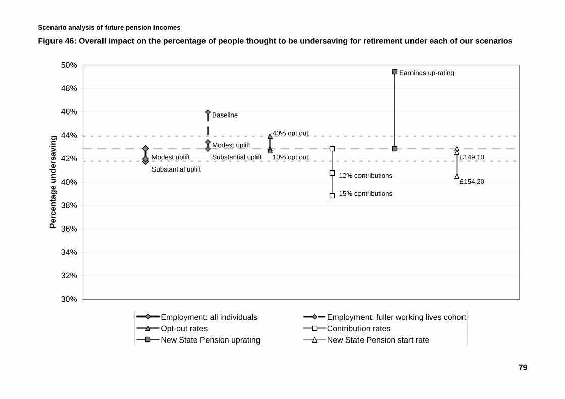
Scenario analysis of future pension incomes
79
Figure 46: Overall impact on the percentage of people thought to be undersaving for retirement under each of our scenarios
30%
32%
34%
36%
38%
40%
42%
44%
46%
48%
50%Pe
rcen
tage
und
ersa
ving
Employment: all individuals Employment: fuller working lives cohortOpt-out rates Contribution ratesNew State Pension uprating New State Pension start rate
£154.20
£149.1010% opt out
40% opt out
15% contributions
12% contributions
Baseline
Substantial uplift
Modest uplift
Substantial uplift
Modest uplift
Earnings up-rating
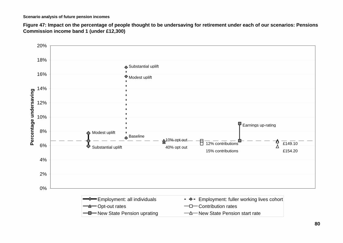
Scenario analysis of future pension incomes
80
Figure 47: Impact on the percentage of people thought to be undersaving for retirement under each of our scenarios: Pensions Commission income band 1 (under £12,300)
0%
2%
4%
6%
8%
10%
12%
14%
16%
18%
20%
Perc
enta
ge u
nder
savi
ng
Employment: all individuals Employment: fuller working lives cohortOpt-out rates Contribution ratesNew State Pension uprating New State Pension start rate
£154.20
£149.1010% opt out
40% opt out15% contributions
12% contributions
Earnings up-rating
Baseline
Substantial uplift
Modest uplift
Substantial uplift
Modest uplift

Scenario analysis of future pension incomes
81
Figure 48: Impact on the percentage of people thought to be undersaving for retirement under each of our scenarios: Pensions Commission income band 2 (£12,300 to £22,700)
15%
20%
25%
30%
35%
Perc
enta
ge u
nder
savi
ng
Employment: all individuals Employment: fuller working lives cohortOpt-out rates Contribution ratesNew State Pension uprating New State Pension start rate
£154.20
£149.10
Earnings up-rating
15% contributions
12% contributions10% opt out
40% opt out
Modest upliftSubstantial uplift
Baseline
Substantial uplift
Modest uplift

Scenario analysis of future pension incomes
82
Figure 49: Impact on the percentage of people thought to be undersaving for retirement under each of our scenarios: Pensions Commission income band 3 (£22,700 to £32,500)
45%
50%
55%
60%
65%
Perc
enta
ge u
nder
savi
ng
Employment: all individuals Employment: fuller working lives cohortOpt-out rates Contribution ratesNew State Pension uprating New State Pension start rate
40% opt out10% opt out
£154.20
£149.10
Earnings up-rating
15% contributions
12% contributions
Baseline
Substantial uplift
Modest upliftSubstantial uplift
Modest uplift

Scenario analysis of future pension incomes
83
Figure 50: Impact on the percentage of people thought to be undersaving for retirement under each of our scenarios: Pensions Commission income band 4 (£32,500 to £52,000)
50%
55%
60%
65%
70%
Perc
enta
ge u
nder
savi
ng
Employment: all individuals Employment: fuller working lives cohortOpt-out rates Contribution ratesNew State Pension uprating New State Pension start rate
10% opt out
£154.20
£149.10
Earnings up-rating
15% contributions
12% contributions
40% opt out
Baseline
Modest uplift
Substantial upliftModest uplift
Substantial uplift

Scenario analysis of future pension incomes
84
Figure 51: Impact on the percentage of people thought to be undersaving for retirement under each of our scenarios: Pensions Commission income band 5 (over £52,000)
55%
60%
65%
70%
75%
Perc
enta
ge u
nder
savi
ng
Employment: all individuals Employment: fuller working lives cohortOpt-out rates Contribution ratesNew State Pension uprating New State Pension start rate
£154.20
£149.10
Earnings up-rating
15% contributions
12% contributions
10% opt out
40% opt out
Baseline
Substantial uplift
Modest uplift
Substantial uplift
Modest uplift

Scenario analysis of future pension incomes
85
Figure 52: Impact on the percentage of people thought to be “substantial” undersavers (less than 50 per cent of target replacement rate achieved) under each of our scenarios
0%
2%
4%
6%
8%
10%
Perc
enta
ge u
nder
savi
ng
Employment: all individuals Employment: fuller working lives cohortOpt-out rates Contribution ratesNew State Pension uprating New State Pension start rate
£154.20
£149.10
Earnings up-rating
15% contributions
12% contributions10% opt out
40% opt outBaseline
Substantial uplift
Modest upliftSubstantial uplift
Modest uplift

Scenario analysis of future pension incomes
86
Figure 53: Impact on the percentage of people thought to be “moderate” undersavers (achieving between 50 and 80 per cent of their target replacement rate) under each of our scenarios
10%
15%
20%
25%
30%
Perc
enta
ge u
nder
savi
ng
Employment: all individuals Employment: fuller working lives cohortOpt-out rates Contribution ratesNew State Pension uprating New State Pension start rate
£154.20
£149.10
Earnings up-rating
15% contributions
12% contributions
10% opt out
40% opt outBaseline
Substantial uplift
Modest upliftModest upliftSubstantial uplift

Scenario analysis of future pension incomes
87
Figure 54: Impact on the percentage of people thought to be “mild” undersavers (achieving between 80 and 100 per cent of their target replacement rate) under each of our scenarios
18%
19%
20%
21%
22%
23%
Perc
enta
ge u
nder
savi
ng
Employment: all individuals Employment: fuller working lives cohortOpt-out rates Contribution ratesNew State Pension uprating New State Pension start rate
£154.20
£149.10
Earnings up-rating
15% contributions
12% contributions40% opt out
10% opt out
Baseline
Substantial uplift
Modest uplift
Substantial uplift
Modest uplift

Scenario analysis of future pension incomes
88
Figure 55: Impact on the percentage of people thought to be undersaving for retirement under each of our scenarios among those reaching State Pension age in the 2020’s
35%
40%
45%
50%
55%
Perc
enta
ge u
nder
savi
ng
Employment: all individuals Employment: fuller working lives cohortOpt-out rates Contribution ratesNew State Pension uprating New State Pension start rate
£154.20
£149.10
Earnings up-rating
15% contributions
12% contributions10% opt out
40% opt out
Baseline
Substantial uplift
Modest upliftModest upliftSubstantial uplift

Scenario analysis of future pension incomes
89
Figure 56: Impact on the percentage of people thought to be undersaving for retirement under each of our scenarios among those reaching State Pension age in the 2030’s
35%
40%
45%
50%
55%
Perc
enta
ge u
nder
savi
ng
Employment: all individuals Employment: fuller working lives cohortOpt-out rates Contribution ratesNew State Pension uprating New State Pension start rate
£154.20
£149.10
Earnings up-rating
15% contributions
12% contributions10% opt out
40% opt out
Baseline
Substantial uplift
Modest uplift
Substantial uplift
Modest uplift

Scenario analysis of future pension incomes
90
Figure 57: Impact on the percentage of people thought to be undersaving for retirement under each of our scenarios among those reaching State Pension age in the 2040’s
35%
40%
45%
50%
55%
Perc
enta
ge u
nder
savi
ng
Employment: all individuals Employment: fuller working lives cohortOpt-out rates Contribution ratesNew State Pension uprating New State Pension start rate
£154.20
£149.10
Earnings up-rating
15% contributions
12% contributions
10% opt out
40% opt out
Baseline
Substantial uplift
Modest uplift
Modest upliftSubstantial uplift

Scenario analysis of future pension incomes
Figure 58: Impact on the percentage of people thought to be undersaving for retirement under each of our scenarios among those reaching State Pension age in the 2050’s
30%
35%
40%
45%
50%
Perc
enta
ge u
nder
savi
ng
Employment: all individuals Employment: fuller working lives cohortOpt-out rates Contribution ratesNew State Pension uprating New State Pension start rate
£154.20
£149.10
Earnings up-rating
15% contributions
12% contributions
10% opt out
40% opt out
Baseline
Substantial uplift
Modest uplift
Modest upliftSubstantial uplift
91