sap predictive analytics: the comprehensive guide · pdf filereading sample this sample...

Reading SampleThis sample chapter demonstrates how to create a clustering model in SAP Predictive Analytics, how to understand its output, and how to apply it to new data. It also provides some information on the concepts behind supervised and unsupervised clustering along with a short description of the mathematical process used to create clusters.

Chabert, Forster, Tessier, Vezzosi

SAP Predictive Analytics: The Comprehensive Guide491 Pages, 2018, $79.95 ISBN 978-1-4932-1592-8

www.sap-press.com/4491

First-hand knowledge.

“Automated Predictive Clustering Models”

Contents

Index

The Authors

https://www.sap-press.com/sap-predictive-analytics_4491/authors/?utm_source=AWS&utm_medium=readingsample&utm_campaign=Browse%20the%20Book&utm_content=1592

271

11

Chapter 11

Automated Predictive Clustering Models

Clustering automatically creates segments of your customers, prod-

ucts, or other business entities. Helping you better understand your

environment, clustering allows you to concentrate and target actions

to a few groups of entities rather than working individually with each

entity.

Clustering is a predictive analytics approach that creates groups of records from your

dataset (called clusters or segments) based on their mathematical closeness. Two

records in the same cluster are more “mathematically similar” than two records in

different clusters, and this similarity is measured by the values of their attributes.

SAP Predictive Analytics provides an automated module for clustering in the Auto-

mated Analytics interface. The module takes care of various tasks for defining and

generating a clustering model and lets you concentrate on higher-value tasks, such as

finding other data to improve the model or brainstorming ideas on how the model

can benefit your business.

The use of clustering can be of a great help when you want to better understand your

business or take appropriate actions to improve the business. The fundamental idea

is that any of your business subjects (your products, customers, employees, depart-

ments, etc.) can be submitted to a clustering analysis, which creates groups that can

then be analyzed as a whole. Practically, you’ll reduce the scope of your analysis from

a lot of individual data points to a just few groups of data points showing similar

characteristics.

Ideally, data points in the same cluster behave similarly and thus should have the

same reaction when you interact with them.

The most typical use for clustering is to create customer groups for marketing cam-

paigns or to enrich a dataset, which is then fed into a classification or regression algo-

rithm. You can take all of your customers and have them grouped into a few clusters.

11 Automated Predictive Clustering Models

272

After analyzing the typical profile of customers in a cluster, you can create a targeted

marketing campaign for that profile.

This approach lets you balance the benefit from creating a personalized campaign

against the cost of conducting a specific campaign for each of your customers.

Other typical uses relate to identifying groups of customers who might churn or

employees who want to leave the company. Internet of Things (IoT) scenarios may

involve identifying which among thousands of input sources, like sensors, have sim-

ilar behaviors.

In this chapter, you’ll learn how to create a clustering model, how to understand its

output, and how to apply it to new data. We’ll also provide some information on the

concepts behind supervised and unsupervised clustering and provide a short

description of the mathematical process used to create clusters.

11.1 The Clustering Approach of Automated Analytics

Automated Analytics has a specific module dedicated to clustering under the

Modeler component. The module simplifies the workflow as much as possible; time-

consuming activities that don’t necessarily improve the model’s quality are auto-

matically taken into account by the tool. Thus, you can concentrate on higher-value

activities. As with the other components in Automated Analytics, a secondary goal is

to speed up the process of defining and creating clustering models to decrease the

cost of predictive modeling and to enable the mass creation of more models. How-

ever, the Automated Analytics approach doesn’t compromise on the final accuracy of

the generated model.

You’ll be able to set various properties of the algorithm that creates the model using

a wizard-like interface, but the bulk of the work will be done for you automatically

without compromising on model quality.

The mathematical approach is described in Section 11.4, but for data scientists, we’ll

just mention that, behind the scenes, the clustering module manages a centroid

method based on the K-Means algorithm.

In Automated Analytics, clustering can be either supervised or unsupervised. When

unsupervised, the clustering analysis puts together data points that are considered

similar with regard to all of their attributes. When supervised, the clusters are

adjusted to provide a distribution that explains their influence on the target variable.

This information is obtained by organizing the input values in groups with a similar

273

11.2 Creating a Clustering Model

11

influence on the target variable. The target can be either a continuous or a nominal

variable, with only two values. As a result, you can interpret the results as though a

regression or classification model. In general, we recommend using supervised clus-

tering because the output better answers your business question and also because

you can reuse the output as an input for a classification model.

Finally, Automated Analytics provides an option defining clusters using SQL state-

ments. This option reduces the mathematical exactitude of the output but allows for

exporting the model into your database for easy processing.


In this section, we’ll explain how to create a clustering model using a sample dataset.

The detailed step-by-step process will help you understand how to use the tool, how

to interpret the output of the model, and how to export your model into an applica-

tion or into a database to be executed on new data.

To illustrate, we’ll use a simple public dataset that can be found at https://archive.ics.

uci.edu/ml/datasets/Wholesale+customers and which is extracted from Abreu, N. (2011).

Analise do perfil do cliente Recheio e desenvolvimento de um sistema promocional.

Mestrado em Marketing, ISCTE-IUL, Lisbon.

The dataset file can also be downloaded from SAP PRESS at www.sap-press.com/4491.

In our example, we’ll suppose that the dataset file, called Wholesale customers

data.csv, is saved in the C:\Predictive directory of the computer running Automated

Analytics on SAP Predictive Analytics desktop.

The Wholesale Customers Dataset

The sample file comes from a study for clustering from the Instituto Universitário de

Lisboa, Portugal, and consists of data about the expenses of customers of a whole-

sale distributor.

The dataset contains 6 continuous integer fields showing the annual expenses of a

customer in different areas (fresh produce, milk, groceries, frozen products, deter-

gents and paper, and, finally, delicatessen).

The Channel nominal field shows if the purchase took place via a retail channel (value 1)

or from a hotel or restaurant (value 2).

The Region nominal field shows if the sale took place in Lisbon (value 1), in Oporto

(value 2), or somewhere else (value 3).


274

To create a clustering model, you’ll perform the following actions:

1. Launch the clustering module and import the data.

2. Analyze the dataset content.

3. Choose the variables to use when defining the model and determine the number

of clusters to generate.

4. Generate the model and analyze the cluster profiles.

5. Apply the model to a dataset.

6. Export the model to an external application for productization.

Our example is an unsupervised clustering model, but in subsequent sections, we’ll

explain the differences between supervised and unsupervised clustering.

In each step, we’ll also provide a description of optional or advanced functionalities

that you can take into account but that won’t be used in our example.

It’s time for you to play with the tool—let’s get started!

11.2.1 Starting the Clustering Module and Importing the Data

After launching Automated Analytics, start the clustering module by clicking on the

Create a Clustering Model entry on the main Modeler page.

On the Select a Data Source page, shown in Figure 11.1, you can use the Browse but-

tons to find the dataset file saved in the C:\Predictive directory.

Figure 11.1 Selecting a Data Source

275


11

After selecting the directory and the file, you can leave the default settings to start

creating your clustering model; however, before going ahead, we’d like to first

explore the various settings available on this page. By changing these settings, you

can import various kinds of datasets and use them in different ways.

The Use File or a Database Table radio button lets you select files from your local

machine or tables from a database. You can control the type of source from the Data

Type dropdown list (where you can select text files, Excel files, SAS or SPSS files, or

database table types). When selecting the Data Base data type, the Browse buttons

will display a list of available ODBC database connections, ask for a username and

password, and let you select a database table.

The Use Data Manager option lets you select an analytical record and a time-stamped

population defined in a database source. How to define these artifacts in the Data

Manager is discussed in Chapter 14.

The wrench icon lets you change the default settings when reading the file. Click

on the icon to open the Settings page, as shown in Figure 11.2.

Figure 11.2 The Import Settings Page


276

You can find detailed information on this page by clicking on the Get Help for this

Panel button or pressing (F1), but the most typical changes that you’ll do here

include the following:

� In the File Settings section:

– Defining a field separator rather than use the default

– Changing the date input format to adapt to the dataset file

� In the Header Line section:

– Setting how many rows at the beginning of a dataset must be skipped so that

the data is read only from the first useful row

Be aware that this page is the first place to try and change settings if you encounter

problems when importing files. For example, when you have date fields listed as text,

separate fields may appear merged, incorrect entries may appear at the beginning of

a dataset, or field names and content may be detected incorrectly.

When you have made the appropriate changes, click the OK button to return to the

Select a Data Source page.

On this page (Figure 11.1), press the loop button to open the Sample Data View

page where you can explore the dataset’s content. By default, the view opens on the

Data tab and presents the first 100 records, as shown in Figure 11.3.

Figure 11.3 The Data Preview Page

277


11

You can show more (or fewer) records by changing the First Row Index and Last Row

Index values in the interface and hitting the refresh button . You can also easily

order by column values by clicking on the column title.

The Statistics tab is useful for more insights into the dataset’s content and to under-

stand if the dataset contains useful data or problematic values.

After selecting the Statistics tab and clicking on the Compute Statistics button, you’ll

have a choice between computing statistics over the entire dataset or only partially.

Then, you’ll see the Variables page, which shows a list of detected fields, their types,

and the number of missing values for each field. More interestingly, in the Category

Frequency tab, shown in Figure 11.4, you can see how variables are distributed across

values.

Figure 11.4 The Category Frequency Tab Showing the Distribution of a Continuous Variable

Nominal variables are displayed with the frequency of each value; continuous vari-

ables are grouped in 20 bins of equal frequency: the larger the bin interval, the lower

frequency for each element inside the bin.


278

Finally, the Continuous Variables tab (Figure 11.5) shows some useful information on

variables with continuous values.

Figure 11.5 Statistics of Continuous Variables

You can see the maximum, minimum, and mean values of and the standard devia-

tion for each variable. All the information in the Statistics tab helps you understand

the quality of the dataset and to check that the data is suitable for the analysis you

want to run.

Click on the Close button to go back to the Select Data Source window (Figure 11.1).

Now, click on the Cutting Strategy… button to select a different cutting strategy than

the default Random Without Test. Information about choosing a cutting strategy can

be found in Chapter 6.

For our example, you don’t have to change any options; you’ll just keep the defaults.

Click on the Next button of the Select a Data Source screen shown in Figure 11.1. You

have now successfully imported the dataset. In the next step, you’ll analyze the data

analyzed by the tool.

279


11

11.2.2 Analyzing the Dataset’s Content

After you have selected a data source, the Data Description page, shown in Figure 11.6,

opens. Click on the Analyze button at the top, and the tool will detect the necessary

information about the dataset fields.

Figure 11.6 The Data Description Page (after Clicking the Analyze Button)

This page shows you the information detected by the tool within the dataset and lets

you modify this information if the automated detection is incorrect or if you want to

personalize how data will be interpreted. This page is important because this infor-

mation controls how variables will be encoded for the model. Good encoding is nec-

essary for the quality and correctness of the resulting model.

In the main table displayed on this page, you can check the information assigned to

each variable and change it when necessary by double-clicking on the cell you want

to modify. The definition of each column is described in Table 11.1.


280

At the top of the page, three tabs give you a better control on how the dataset is

described, as follows:

� The Main tab (Figure 11.6) lets you automatically analyze the dataset by clicking on

the Analyze button. The most important elements on this tab are as follows:

– The Save Description button lets you save the actual description of the dataset

in a file or in a database table. The opposite, the Load Description button, opens

Column Description

Index This column is just a numerical index to give an ID number to each variable.

Name This column displays the name of the variable as found in the dataset.

Storage This column displays the type of the variable (Number, Integer, String, Date,

Datetime, or Angle). You can change this value by double-clicking on the

table cell.

Value This column displays the content type of the variable (Continuous, Nominal,

Ordinal, or Textual). The value type defines the way that the variable is

encoded for the model. For more information, see Chapter 6. You can change

this value by double-clicking on the table cell.

Key This column shows whether the variable is a primary key of the dataset

(value 1) or a secondary key (value 2). Variables that are not keys have a value

of 0. You can change this value by double-clicking on the table cell.

Order This column shows whether the variable has an order (value 1) and can be

used in an Order By clause. You can change this value by double-clicking on

the table cell.

Missing Provides the value to be used when the variable is null. By default, the tool

will use the KxMissing label, but you can enter a text to override the default.

Group This column displays the group to which a variable belongs, if any. You can

put multiple variables in the same group if, together, they provide a single

piece of information. Variables in the same group are not crossed when

working with models of order 2 or bigger. You can manually set the group

information by double-clicking in the cell and providing a group name.

Description This column provides a text description of the variable.

Structure This button opens the Structure definition page where you can override the

automated encoding of the variables.

Table 11.1 Description Columns in the Dataset

281


11

a description that was previously saved and applies the description to the data-

set. Usually, a description is made for a dataset and applied to the same dataset

when loaded again.

– The Save in Variable Pool button lets you save the description of a single vari-

able or of all the variables. The information in the variable pool is then automat-

ically applied across different datasets each time a variable with the name

found in the variable pool is encountered. This technique can be used to share

definitions across datasets. The Remove from Variable Pool button takes away

the description of the selected variable from the pool.

– Finally, the View Data button opens the Sample Data View page, which we dis-

cussed in Section 11.2.1. Clicking on the Properties button simply resumes the

variable description already displayed in the table but in a nicer format.

� The Edition tab, shown in Figure 11.7, gives you control over the Storage, Value,

Missing, and Group columns of the description by clicking the respective buttons.

Three important buttons on this tab are as follows:

Figure 11.7 The Edition Tab of the Data Description Page

– The Translate categories button lets you provide a translation of the values of

a variable. You can associate to each value a text in different languages. This

information is useful when doing a textual analysis of the information where

you want to make sure that different words are associated to the same concept

in different languages.

– The Composite Variables button lets you associate two values as the latitude

and longitude of a single position variable. The two source variables must be of

storage Angle. When associated, the two variables will always be used together.

With the same button, you can also force some variables to be crossed together

when creating a predictive model.

– The Set Group button lets you add multiple variables to the same group.


282

� The last tab, the Structures tab, is shown in Figure 11.8. This tab gives the same con-

trol that you have when double-clicking on the Structure column in the main

table. A structure can be used to override the automated encoding of the variable

provided by the tool.

Figure 11.8 The Structures Tab of the Data Description Page

You can define a new structure for a variable clicking on the New Structure button.

For nominal variables, you can define how the various values of the variable

(named Categories in the interface) must be grouped together. For ordinal and

continuous variables, you can define the number of intervals (the Band Count) and

the content of each interval to be used for the encoding. When editing a structure,

you can also open the Advanced tab, as shown in Figure 11.9. Here, you have the fol-

lowing two options:

Figure 11.9 The Advanced Tab in the Structure Definition Interface

– Selecting the Enable the target based optimal grouping performed by K2C

checkbox tells the tool take into account both the structure you defined and the

structure automatically generated. The tool will determine the best structure

for the model.

– Selecting the Uses Natural Encoding checkbox tells the tool to also use variables

directly without any encoding based on the target.

283


11

As shown in Figure 11.8, the From Statistics, From Variable, and From Model but-

tons automatically fill in the structure using information already available in the

statistical distribution, in the variable pool, or in another model. You can override

the content after loading it.

Going back in the main Data Description page (Figure 11.6), notice the button and the

Add Filter in Dataset checkbox. If you select the checkbox, you’ll be asked on the next

page to define a filter on the dataset itself. You could, as for our example, limit the

analysis to a single value of the Channel field or for a single Region. The filter here is

useful when using Predictive Factory because you can tell the application to auto-

matically change the value of this filter and hence automatically produce multiple

models, one for each value chosen. This workflow is described in more detail in Chap-

ter 9. For the time being, do not set any filter. For our example, you don’t have to

modify any default values after clicking the Analyze button. Click Next to go to the

page for selecting the variables to be used to build the model.

11.2.3 Choosing the Variables and Setting the Model Properties

In this step, you’ll provide a list of variables to consider and, optionally, change the

main parameters for how the model is defined. On the Selecting Variables page

shown in Figure 11.10, you’ll set which variables the model should use.

Figure 11.10 The Selecting Variables Page


284

To move a variable from one group to another, click on its name and use the right or

left arrow buttons. Variables can be placed into one of four groups, as described in

Table 11.2.

For our example, you’ll use the default content of the page when you open it. In other

words, the Target Variables group will remain empty and an unsupervised clustering

will be performed.

Click Next at the bottom of the page, and the Summary of Modeling Parameters page

will open (Figure 11.11). On this page, you’ll find the following options:

� At the top of the page, the Model Name and Description fields let you enter a name

and information you want to share about the model. The read-only section with

the blue background quickly summarizes some of the previous choices you made.

Group Description

Explanatory Variables Selected The variables you place in this group describe and explain

your model. For clustering, place all variables that you

want to consider as dimensions for your analysis of this

group.

Target Variables The variables you place in this group will be used as

targets for supervised clustering. Each variable creates a

different model. No variables in this panel means that the

tool will use unsupervised clustering.

Weight Variables The variables you place in this group provide different

weights to the record where they belong. For example, a

value of “3” for a weight variable of a record means the

tool will count the record three times when generating

the model. You can use this variable to skew the model

definition using the records you consider more important.

Excluded Variables The variables you place in this group will not be consid-

ered for the model. These variables are usually indexes or

IDs or variables that are highly correlated to other vari-

ables in the explanatory group. Two highly correlated

variables don’t carry additional information and can even

decrease the quality of the model.

Table 11.2 The Roles of Variables in the Model

285


11

� The Find the best number of clusters in this range fields lets you choose the mini-

mum and maximum number of clusters to be considered by the tool. Putting the

same number in both boxes actually provides a fixed value. The values set in these

fields are only requests because the final result may contain fewer clusters than

you requested (more clusters might be unstable). Also, an additional cluster than

what you requested may appear: This cluster contains all items that could not be

logically placed in the other clusters.

� The Calculate SQL Expressions checkbox is very important: When not selected, the

tool defines the best possible clusters using the mathematical approach described

in Section 11.4. When the checkbox is selected, the tool adjusts the clusters so that

they can be expressed using SQL sentences. The mathematical accuracy of the

cluster might be reduced, but you’ll be able to export the model into a database to

apply the model to new data.

Figure 11.11 The Summary of Model Parameters Page


286

� The Autosave button lets you define the location where the model will be saved

automatically (usually the model is saved after it is generated, but the autosave

option can be useful if the model is taking a long time to generate). Once gener-

ated, the model will be automatically saved at the location you specify.

� Clicking on the Advanced button opens the Specific Parameters of the Model page

where you can override some important parameters. You must be careful on this

page because changing parameters might not enhance the quality of the model

and might increase its generation time. You can decide whether you want to

obtain a detailed description of the influence of the variables on the model by

selecting the Calculate Cross Statistics box. If you are conducting a supervised

clustering, you can define the desired value of the target variable by setting it in

the Target Key column. By default, this value is the least frequent value in the data-

set. The Distance dropdown menu lets you override the definition of distance

between two records in the cluster definition according to the settings described

in Table 11.3.

Finally, the Encoding Strategy lets you choose whether you’ll use the default

encoding of variables; if you want to force an Unsupervised encoding, even during

supervised clustering; or if you want to force a Uniform encoding where all vari-

ables are distributed at regular interval (i.e., between −1 and +1).

For our example, do not change any advanced settings.

Set the number of clusters between 3 and 5 on the main page (Figure 11.11) and keep

the Calculate SQL Expressions checkbox selected, then click on the Generate button

to start the model definition process.

Setting Description

System Determined This setting keeps allows uses the best distance methodology auto-

matically determined by the tool after the dataset is read.

City Block This setting defines distance as the sum of the absolute differences

of the coordinates of the points.

Euclidean This setting returns the square root of the sum of the square differ-

ences of the coordinates.

Chessboard Also known as “Manhattan style,” this setting uses the maximum

value of the absolute difference of the coordinates.

Table 11.3 Various Distance Definitions Available for Clustering

287


11

11.2.4 Generating the Model and Analyzing the Cluster Profiles

After clicking the Generate button, a new page will open showing some logs of the

ongoing calculations. The information is displayed and refreshed quickly, and you

probably won’t be able to read it. Don’t worry, if something goes wrong, you’ll be

notified. If all goes well, a detailed log of the performed actions will open in the sub-

sequent page, the Training the Model page, which shows by default the Model Over-

view (shown in Figure 11.12).

Figure 11.12 The Model Overview after Generation

You can choose the style of report to display with the Report Type dropdown menu at

the top of the page. The Model Overview style is shown by default, and we recom-

mend using it. The Executive Report style is useful for a detailed summary of the

model, but you’ll find the same information and more in a better interface afterwards.


288

From this overview, notice that you have 440 records in the dataset and that 8.25% of

them have not been assigned to any cluster. (This value is quite high but should be

expected if you had selected the Calculate SQL Expressions checkbox, which tends to

build clusters that are less able to include all available records while keeping the SQL

sentence readable.)

Also notice that 14.19% of records were overlapping, meaning they appear in more

than one cluster. The generation of the SQL takes this overlap into account, and the

final version of the model will ensure that a record appears only in one cluster. Know-

ing the number of overlapping records can help you understand if the generated

clusters are different (no overlaps) or similar (many overlaps).

Finally, notice that, in the end, only 3 clusters were generated. At similar quality, the

tool generates the minimum number of clusters requested so as to simplify the

debriefing and usage of the model.

Click Next to enter in the debriefing and model application interface called the Using

the Model page, as shown in Figure 11.13.

Figure 11.13 Main Interface to Debrief and Apply the Model after Generation

From this page, you can display the model information to better understand how the

model was built, apply the model on new data, and save and export the model into a

database so that the model can be executed in an external application.

289


11

Your first task is to understand what kind of content has been put in each cluster.

Click on the Cluster Profiles link, and the relevant debriefing page will open, as shown

in Figure 11.14.

Figure 11.14 The Cluster Profiles Page

The top table shows a list of all clusters and the percentages they represent. In our

example, Cluster 1 contains 28.57% of the records of the dataset.

When you click on a cluster line on the table, you’ll see at the bottom a bar chart rep-

resenting how that cluster population is distributed by variable. By default, the dis-

play shows the variables with the highest variation for each cluster (in this case, the

Frozen variable for Cluster 1).


290

In the graph, the red bars represent how the total population of the dataset is distrib-

uted over the various values or intervals of the variable. The blue bars show how the

population of the selected cluster is distributed on the same variables. If a blue bar is

higher than the red bar, the cluster population has, in terms of percentage, more

records for that value than the total population. If the red bar is higher than the blue

bar, then the cluster population is underrepresented for that value.

In Figure 11.14, notice that Cluster 1 contains many records with low Frozen values

and no records with high values, while the global population overall is equally dis-

tributed over the same variable. In other words, customers in Cluster 1 spend less on

frozen food than the global average population.

Clicking on another cluster on the table changes the display on the bottom, always

showing the variable that changes the most for that cluster.

You can see how the same variable is distributed across various clusters by checking

the Freeze Variable checkbox and then changing the cluster selection.

Looking at this representation, you can easily see the different profiles of each clus-

ter. One useful approach is to build a qualitative matrix to help you visualize all the

cluster profiles in a single place, which is possible when you have a limited number of

clusters and a limited number of variables.

Using our sample, you can build a matrix, as in Table 11.4, where low and high mean

that the cluster presents a low or high level of expenses in the specific area, while

homogeneous means that a strong bias does not exist.

Cluster 1 Cluster 2 Cluster 3

Frozen Low High Mid-Low

Delicatessen Low Homogeneous Mid-High

Fresh Mid-Low Mid-High Homogeneous

Grocery Mid-Low Mid-Low High

Milk Homogeneous Mid-Low High

Detergent/Paper Homogeneous Mid-Low High

Channel Homogeneous Retail Hotel/Restaurant

Region Homogeneous Homogeneous Homogeneous

Table 11.4 A Qualitative Matrix Showing the Profile of Each Cluster

291


11

From this table, you could decide to run a marketing campaign that divides your cus-

tomers in two groups. For Cluster 2, you can run a campaign to propose more fresh

and frozen food to retail customers; for Cluster 3, a campaign for groceries, milk, and

detergents to hotels and restaurants. The profile of Cluster 1 is a lot less diversified

and seems to have, in general, a low impact on purchases. Thus, you might want not

to spend money on specific marketing campaigns for that group, or you might run a

generic campaign. You can also see that Region is not a discriminatory variable:

Homogeneous across all clusters, this variable is not really important for your seg-

mentation.

You can also have a graphical representation of the cluster profiles by selecting the

Cluster Summary link on the Using the Model page (Figure 11.13).

The Cluster Summary page (Figure 11.15) compares all the clusters over 3 measures

that you can select using the X axis , Y axis , and Size buttons at the top.

Figure 11.15 The Cluster Summary Page


292

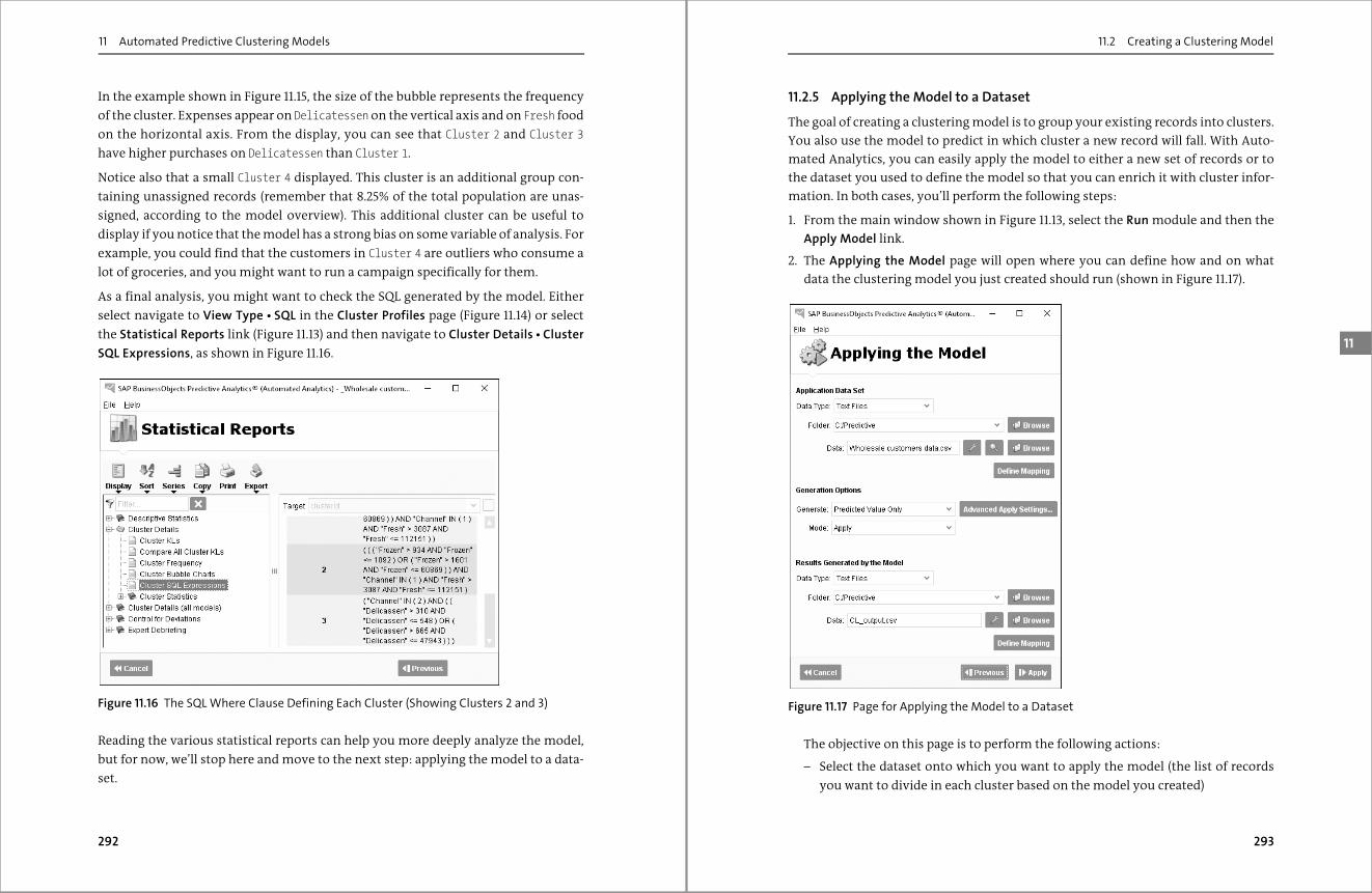
In the example shown in Figure 11.15, the size of the bubble represents the frequency

of the cluster. Expenses appear on Delicatessen on the vertical axis and on Fresh food

on the horizontal axis. From the display, you can see that Cluster 2 and Cluster 3

have higher purchases on Delicatessen than Cluster 1.

Notice also that a small Cluster 4 displayed. This cluster is an additional group con-

taining unassigned records (remember that 8.25% of the total population are unas-

signed, according to the model overview). This additional cluster can be useful to

display if you notice that the model has a strong bias on some variable of analysis. For

example, you could find that the customers in Cluster 4 are outliers who consume a

lot of groceries, and you might want to run a campaign specifically for them.

As a final analysis, you might want to check the SQL generated by the model. Either

select navigate to View Type � SQL in the Cluster Profiles page (Figure 11.14) or select

the Statistical Reports link (Figure 11.13) and then navigate to Cluster Details � Cluster

SQL Expressions, as shown in Figure 11.16.

Figure 11.16 The SQL Where Clause Defining Each Cluster (Showing Clusters 2 and 3)

Reading the various statistical reports can help you more deeply analyze the model,

but for now, we’ll stop here and move to the next step: applying the model to a data-

set.

293


11

11.2.5 Applying the Model to a Dataset

The goal of creating a clustering model is to group your existing records into clusters.

You also use the model to predict in which cluster a new record will fall. With Auto-

mated Analytics, you can easily apply the model to either a new set of records or to

the dataset you used to define the model so that you can enrich it with cluster infor-

mation. In both cases, you’ll perform the following steps:

1. From the main window shown in Figure 11.13, select the Run module and then the

Apply Model link.

2. The Applying the Model page will open where you can define how and on what

data the clustering model you just created should run (shown in Figure 11.17).

Figure 11.17 Page for Applying the Model to a Dataset

The objective on this page is to perform the following actions:

– Select the dataset onto which you want to apply the model (the list of records

you want to divide in each cluster based on the model you created)


294

– Define the format of the output you want to obtain

– Choose where to save the output information

3. Select your dataset in the top section called Application Data Set. The same func-

tionality for selecting a data source was discussed earlier in Section 11.2.1. An addi-

tional button, Define Mappings, lets you specify the corresponding fields between

the application dataset and the fields you used to create the model if the field

names differ.

4. In the Generation Options section, choose the format of the output. In the Gener-

ate dropdown menu, choose from four output templates or to define a custom

formatting. The possible options are listed in Table 11.5.

Option Description

Predicted Value Only The output contains two columns only: the ID of the record

in the dataset and the name of the cluster where it has

been assigned.

Cluster ID Disjunctive coding The output contains a column with the ID of the record

and a column for each cluster. In each cluster column, the

value is 1 if the record is in the cluster and 0 if not.

Cluster ID Disjunctive Coding

(+ Copy Data Set)

This option results in the same output as above but addi-

tionally includes the complete record information (the ID,

the cluster disjunctive columns, and a column for each vari-

able of the dataset). This output is well formed and can be

used as an input for a classification or regression analysis.

Cluster ID Target Mean This option is available only for supervised clustering. This

option includes an additional output column that shows

the target mean of the cluster on the target variable (thus

measuring how “close” the cluster is to the target vari-

able). This information can be useful on its own as well as

an input for further classification analysis.

Advanced Apply Setting Clicking the Advanced Apply Settings… button lets you

control the output in detail. For example, you can add, for

each cluster and record, statistical information on the

probability of belonging to the cluster, the distance from

the centroid, and other information.

Table 11.5 Clustering Output Options

295


11

The disjunctive options, specifically with the copied dataset, can be quite useful to

feed the clustering output into a classification model: By running a classification,

you’ll gain a better understanding of the content of each cluster.

5. From the Mode dropdown menu, decide if you really want to generate an output

(select Apply) or if you just want to update the statistics information visible in the

model statistics set of documents (select Update Only Statistics).

6. Finally, in the Results Generated by Model section of Figure 11.17, you can define

where to save the generated output. This section has the same functionality of the

top section where you select the input dataset.

For our example, select the Wholesale customers data.csv as the application dataset,

leave the Predicted Value only output option, and add the name of a new file to create

in the resulting output (you can use any name, but we called ours CL_output.csv in

Figure 11.17).

Click on the Next button to create the output file, which you can read by clicking on

the View Output button on the following page.

Now, you’ve seen how to apply the model onto a dataset using the Automated Ana-

lytics interface, but most of the time, you’ll need to apply the model directly onto

data in a database or within a workflow of an external application. For these cases,

you’ll export the model as we discuss in the next section.

11.2.6 Saving and Exporting the Model

To reuse the model after generation, you’ll need to save the model by going to the

Save/Export module on the main Using the Model page (Figure 11.13) and clicking the

Save Model link. A new page will open, giving you the choice of saving the model as a

file or in a database. The model can now be reopened in Automated Analytics and

also in Predictive Factory. You can use Predictive Factory to automatically schedule

the refreshing or the application of the model. If you added a filter, as we did in Sec-

tion 11.2.2, you can then tell Predictive Factory how to replace the filter to generate

multiple models.

If you want to export the model into an external application, select the Generate

Source Code link in the Save/Export module. The Generating Code page will appear

(as shown in Figure 11.18).


296

Figure 11.18 The Generating Code Page to Export the Model to Other Applications

Using this screen, you can generate code or a function that requires as input the vari-

ables used for the model generation and that returns as output the cluster into which

the input fits. You can use this code, for example, in an application that takes values

for a customer to obtain the group into which a customer is categorized. Using this

interface, you’ll select the type of code you need for your application (typically the

development language of your application) and the name of the text file where you

want the code to be generated, as follows:

� The Target to be used dropdown list is enabled only when you run a supervised

clustering model. This list lets you choose the target variable for generating scores

and estimates.

� The Code type dropdown list lets you choose the language of the code to be gen-

erated. Many different languages are available, from generic SQL, to database-

specific SQL, to JAVA, C, and C++, and even code for SAS applications.

� In the Output section, you’ll name the text file where you want the code to be gen-

erated. You also have the option of displaying the code when finished.

297

11.3 Supervised and Unsupervised Clustering

11

After your choices have been made, click on the Generate button, and the code will be

written. Depending on the code option chosen, you might be prompted to provide

the $Dataset and $Key values (respectively, the dataset table that contains the data

onto which you want to apply the clustering model and the column in the table that

represents the IDs of the records).

After the file is generated, you can open it, copy the code, and paste it into your appli-

cation. Minimal adjustments might be required to integrate the generated code cor-

rectly with your previously existing code.

Play with the various code types to see some examples of outputs. In Figure 11.18, we

used settings to generate a file containing SQL code optimized for SAP HANA.

You’ve now created the model, applied it to new data, and even exported it into

another application. In the remaining sections of this chapter, you’ll learn more

about supervised clustering and the clustering module’s mathematical approach.

11.3 Supervised and Unsupervised Clustering

The example shown so far demonstrated unsupervised clustering: In the Selecting

the Variables page (Figure 11.10), you didn’t enter a target variable. If you had selected

a target variable (or more than one), then a supervised clustering would have been

performed.

With supervised clustering, all the explanatory variables are encoded to provide bet-

ter explanations of the target variable, using the same target mean-based encoding

found in classification and regression models. Moreover, the target variable was not

used to define the cluster when you generate the SQL code. As a result, you obtain a

model that tries not only to define groups of records but also tries to create groups

that explain the value of the target variable or have a distribution that provides a bet-

ter view on how a cluster relates to the target. This technique can be tailored to

answer specific business questions and is a clustering methodology well suited for

operational use.

In our example, you might want to do a supervised clustering using Channel as the

target variable. Perhaps you want to create better marketing campaigns for retail cus-

tomers or hotel and restaurant customers. To run the test, just go back to the page

shown in Figure 11.10, add the Channel variable as a target key, and then rebuild the

model using the same settings (e.g., same number of clusters between 3 and 5).


298

Now, when you look at the model overview, notice the sections related to the target

key, as shown in Figure 11.19.

Figure 11.19 Model Overview with Additional Information for Supervised Clustering

The good predictive power of 0.87 (87%) shows that the chosen clusters are actually

providing a quite accurate prediction of the target channel.

Looking at the cluster profiles (an example is shown in Figure 11.20), notice that Clus-

ter 4 and 5 are quite interesting for your task.

Figure 11.20 Cluster Profiles in Supervised Clustering

299

11.4 The Data Science behind Automated Clustering Models

11

Cluster 4 and 5 have the most records. The population of Cluster 4 consists mainly of

retail customers (channel is 1), while the population of Cluster 5 consists of hotels and

restaurants (channel is 2). Looking at the other variables, notice that Cluster 4 mem-

bers have low expenses on Milk, Paper, and Groceries—exactly the opposite of

members of Cluster 5. This kind of information might lead you to build specific, cus-

tomized marketing campaigns just for the members of those two clusters. With

supervised clustering, the tool generates all the statistical information related to the

category’s significance.

11.4 The Data Science behind Automated Clustering Models

Automated Analytics uses a K-Means algorithm based on centroids to calculate the

clusters.

The process is iterative:

1. At the beginning, a number of random points are generated (one point for each

cluster you want); these points are called centroids.

2. Then, clusters are created by the points in the dataset that are closer to each cen-

troid, based on the definition of distance you chose (as discussed in Section 11.2.3).

3. Then, for each cluster, the algorithm calculates the center as the point that mini-

mizes the sum of distances from each point.

4. The centroid is then assigned to the newly calculated center. If the old centroid and

the new center coincide, you have a stable solution and the process ends. If instead

the centroid and the new center don’t match, the iteration starts again from step 2.

In Automated Analytics, you have the option of asking for the generated SQL code to

define the clusters. If this option is enabled, an additional step occurs after the clus-

ters are defined where the clusters are adjusted slightly so that they can be expressed

with an SQL where clause, which is usually less expressive than a mathematical func-

tion. These adjustments might cause some points to go outside a cluster (and these

points are considered unassigned records), and some points might fall into two dif-

ferent clusters. In this case, the algorithm automatically modifies the SQL where

clause to avoid having points in multiple clusters.


300

11.5 Summary

In this chapter, we discussed what is clustering and how to successfully define a clus-

tering model with Automated Analytics in SAP Predictive Analytics. You learned

about most of the options for customizing the model to best fit your needs, and

you’ve seen the difference between unsupervised and supervised clustering (the rec-

ommended option).

In the next chapter, we’ll keep working with Automated Analytics and learn how to

build a Social Network Analysis model.

7

Contents

Preface ..................................................................................................................................................... 17

PART I Getting Started

1 An Introduction to Predictive Analytics 23

1.1 The Importance of Predictive Analysis ....................................................................... 24

1.2 Predictive Analysis: Prescriptive and Exploratory ................................................ 26

1.2.1 The Fundamental Idea ........................................................................................ 26

1.2.2 Prescriptive Analytics .......................................................................................... 28

1.2.3 Exploratory Analytics .......................................................................................... 29

1.2.4 Prescriptive vs. Exploratory Analytics ............................................................ 30

1.3 Preparing for a Successful Predictive Analysis Project ....................................... 32

1.3.1 Stakeholders ........................................................................................................... 32

1.3.2 Business Case: Objectives and Benefits ........................................................ 34

1.3.3 Requirements ........................................................................................................ 35

1.3.4 Execution and Lifecycle Management .......................................................... 36

1.4 Industry Use Cases .............................................................................................................. 37

1.5 Summary ................................................................................................................................. 39

2 What Is SAP Predictive Analytics? 41

2.1 Building Predictive Models with SAP Predictive Analytics ............................... 41

2.2 Automated Analytics and Expert Analytics ............................................................. 42

2.3 Mass Production of Predictive Models with the Predictive Factory ............. 43

2.3.1 Result Production ................................................................................................. 43

2.3.2 Model Control ........................................................................................................ 43

Contents

8

2.3.3 Model Retraining ................................................................................................. 44

2.3.4 Mass Production of Predictive Models ......................................................... 45

2.4 Data Preparation ................................................................................................................. 45

2.5 Additional SAP Predictive Analytics Capabilities .................................................. 47

2.6 Summary ................................................................................................................................. 48

3 Installing SAP Predictive Analytics 49

3.1 Recommended Deployments ........................................................................................ 50

3.2 Installing the SAP Predictive Analytics Server ....................................................... 51

3.2.1 Downloading the SAP Predictive Analytics Server ................................... 51

3.2.2 System Requirements ........................................................................................ 52

3.2.3 Installing the SAP Predictive Analytics Server ............................................ 53

3.2.4 Post-Installation Steps ....................................................................................... 54

3.3 Installing the SAP Predictive Analytics Client ........................................................ 57

3.3.1 Downloading the SAP Predictive Analytics Client ..................................... 58


3.3.3 Installation Steps ................................................................................................. 59

3.3.4 Checking the Installation .................................................................................. 60

3.3.5 Starting the Client on Linux Operating Systems ....................................... 60

3.4 Installing the Predictive Factory ................................................................................... 61

3.4.1 Downloading the Predictive Factory ............................................................. 61




3.5 Installing SAP Predictive Analytics Desktop ........................................................... 71




3.6 SAP HANA Installation Steps ......................................................................................... 74

3.7 Summary ................................................................................................................................. 75

9

Contents

4 Planning a Predictive Analytics Project 77

4.1 Introduction to the CRISP-DM Methodology .......................................................... 78

4.2 Running a Project ................................................................................................................ 81

4.2.1 Business Understanding .................................................................................... 81

4.2.2 Data Understanding ............................................................................................ 85

4.2.3 Data Preparation .................................................................................................. 87

4.2.4 Modeling ................................................................................................................. 93

4.2.5 Evaluation ............................................................................................................... 96

4.2.6 Deployment ............................................................................................................ 97

4.3 Summary ................................................................................................................................. 100

PART II The Predictive Factory

5 Predictive Factory 103

5.1 Predictive Factory: End-to-End Modeling ................................................................. 103

5.2 Creating a Project ................................................................................................................ 105

5.3 External Executables .......................................................................................................... 107

5.4 Variable Statistics ................................................................................................................ 110

5.5 Summary ................................................................................................................................. 110

6 Automated Predictive Classification Models 111

6.1 Introducing Classification Models .............................................................................. 112

6.1.1 The Classification Technique ............................................................................ 112

6.1.2 Step-by-Step Classification Example ............................................................. 114

6.2 Creating an Automated Classification Model ......................................................... 115

6.2.1 Prerequisites ........................................................................................................... 115

6.2.2 Creating the Data Connections and the Project ........................................ 116

6.2.3 Creating the Model .............................................................................................. 117

Contents

10

6.3 Understanding and Improving an Automated Classification Model ........... 123

6.3.1 Understanding an Automated Classification Model ............................... 123

6.3.2 Improving an Automated Classification Model ......................................... 135

6.4 Applying an Automated Classification Model ....................................................... 139

6.4.1 Prerequisites .......................................................................................................... 139

6.4.2 Applying a Classification Model ...................................................................... 143

6.5 The Data Science behind Automated Predictive Classification Models ..... 149

6.5.1 Foundations of Automated Analytics ........................................................... 150

6.5.2 Automated Data Preparation .......................................................................... 160

6.5.3 Automated Data Encoding ............................................................................... 164

6.6 Summary ................................................................................................................................. 172

7 Automated Predictive Regression Models 173

7.1 Introducing Regression Models .................................................................................... 173

7.2 Creating an Automated Regression Model ............................................................. 174

7.3 Understanding and Improving an Automated Regression Model ................ 179

7.3.1 Understanding an Automated Regression Model .................................... 179

7.3.2 Improving an Automated Regression Model .............................................. 183

7.4 Applying an Automated Regression Model ............................................................ 184

7.4.1 Safely Applying an Automated Regression Model .................................... 184

7.4.2 Applying an Automated Regression Model ................................................ 186

7.5 Summary ................................................................................................................................. 191

8 Automated Predictive Time Series Forecasting Models 193

8.1 Creating and Understanding Time Series Forecast Models ............................. 194

8.1.1 Creating and Training Models ......................................................................... 195

8.1.2 Understanding Models ...................................................................................... 202

11

Contents

8.1.3 Saving Time Series Forecasts ............................................................................ 206

8.1.4 Increasing Model Accuracy ................................................................................ 210

8.2 Mass Producing Time Series Forecasts ....................................................................... 214

8.3 Productizing the Forecast Model .................................................................................. 221

8.4 The Data Science behind Automated Time Series Forecasting Models ...... 227

8.4.1 Data Split ................................................................................................................. 227

8.4.2 De-trending ............................................................................................................ 228

8.4.3 De-cycling ................................................................................................................ 229

8.4.4 Fluctuations ............................................................................................................ 230

8.4.5 Smoothing .............................................................................................................. 230

8.4.6 Model Quality ........................................................................................................ 230

8.5 Summary ................................................................................................................................. 231

9 Massive Predictive Analytics 233

9.1 Deploying Predictive Models in Batch Mode .......................................................... 234

9.1.1 Deploying Times Series Forecasting Models ............................................... 234

9.1.2 Deploying Classification/Regression Models .............................................. 237

9.2 Model Quality and Deviation ........................................................................................ 241

9.2.1 Model Deviation Test Task Parameters ........................................................ 242

9.2.2 Model Deviation Test Task Outputs .............................................................. 242

9.3 Automatically Retraining Models ............................................................................... 244

9.3.1 Defining a Model Retraining Task .................................................................. 244

9.3.2 Model Retraining Task Outputs ....................................................................... 247

9.4 Scheduling and Combining Massive Tasks .............................................................. 250

9.4.1 Scheduling Tasks Independently ..................................................................... 251

9.4.2 Event-Based Scheduling ..................................................................................... 253

9.5 Deploying Expert Analytics Models ............................................................................ 253

9.6 Summary ................................................................................................................................. 256

Contents

12

PART III Automated Analytics

10 Automated Analytics User Interface 259

10.1 When to Use Automated Analytics ............................................................................. 259

10.2 Navigating the User Interface ....................................................................................... 260

10.3 Exploring the Automated Analytics Modules ........................................................ 264

10.3.1 Data Manager ....................................................................................................... 264

10.3.2 Data Modeler ......................................................................................................... 265

10.3.3 Toolkit ...................................................................................................................... 266

10.4 Summary ................................................................................................................................. 269

11 Automated Predictive Clustering Models 271

11.1 The Clustering Approach of Automated Analytics ............................................... 272

11.2 Creating a Clustering Model .......................................................................................... 273

11.2.1 Starting the Clustering Module and Importing the Data ....................... 274

11.2.2 Analyzing the Dataset’s Content .................................................................... 279

11.2.3 Choosing the Variables and Setting the Model Properties .................... 283

11.2.4 Generating the Model and Analyzing the Cluster Profiles .................... 287

11.2.5 Applying the Model to a Dataset .................................................................... 293

11.2.6 Saving and Exporting the Model .................................................................... 295

11.3 Supervised and Unsupervised Clustering ................................................................. 297

11.4 The Data Science behind Automated Clustering Models .................................. 299

11.5 Summary ................................................................................................................................. 300

12 Social Network Analysis 301

12.1 Terminology of Social Network Analysis .................................................................. 302

12.2 Automated Functionalities of Social Network Analysis .................................... 303

12.2.1 Node Pairing .......................................................................................................... 304

12.2.2 Communities and Roles Detection ................................................................ 304

13

Contents

12.2.3 Social Graph Comparison .................................................................................. 305

12.2.4 Bipartite Graphs Derivation and Recommendations ............................... 305

12.2.5 Proximity ................................................................................................................. 305

12.2.6 Path Analysis .......................................................................................................... 306

12.3 Creating a Social Network Analysis Model .............................................................. 306

12.3.1 Starting the Module and Importing the Dataset ....................................... 308

12.3.2 Defining the Graph Model to Build ................................................................ 310

12.3.3 Adding More Graphs ........................................................................................... 314

12.3.4 Setting Community, Mega-hub, and Node Pairing Detection .............. 315

12.3.5 Providing Descriptions of Nodes ..................................................................... 320

12.4 Navigating and Understanding the Social Network Analysis Output ......... 323

12.4.1 Understanding Model Quality from the Model Overview ...................... 323

12.4.2 Navigating into the Social Network ............................................................... 328

12.4.3 Applying the Model ............................................................................................. 336

12.5 Colocation and Path Analysis Overview .................................................................... 340

12.5.1 Colocation Analysis .............................................................................................. 340

12.5.2 Frequent Path Analysis ....................................................................................... 344

12.6 Conclusion .............................................................................................................................. 346

13 Automated Predictive Recommendation Models 347

13.1 Introduction ........................................................................................................................... 348

13.1.1 Basic Concepts ....................................................................................................... 348

13.1.2 Datasets ................................................................................................................... 349

13.1.3 Recommended Approaches .............................................................................. 351

13.2 Using the Social Network Analysis Module ............................................................. 353


13.2.2 Understanding the Model ................................................................................. 358


13.3 Using the Recommendation Module .......................................................................... 368


13.3.2 Understanding the Model ................................................................................. 369


13.4 Using the Automated Predictive Library .................................................................. 374

13.5 Summary ................................................................................................................................. 375

Contents

14

14 Advanced Data Preparation Techniques with the Data Manager 377

14.1 Data Preparation for SAP Predictive Analytics ...................................................... 377

14.2 Building Datasets for SAP Predictive Analytics .................................................... 379

14.2.1 Datasets .................................................................................................................. 379

14.2.2 Methodology ......................................................................................................... 380

14.3 Creating a Dataset using the Data Manager .......................................................... 381

14.3.1 Creating Data Manager Objects ..................................................................... 383

14.3.2 Merging Tables ..................................................................................................... 391

14.3.3 Defining Temporal Aggregates ....................................................................... 394

14.3.4 Using the Formula Editor .................................................................................. 398

14.4 Additional Functionalities ............................................................................................... 400

14.4.1 Visibility and Value .............................................................................................. 400

14.4.2 Domains .................................................................................................................. 401

14.4.3 Documentation .................................................................................................... 402

14.4.4 Data Preview and Statistics .............................................................................. 403

14.4.5 Generated SQL ...................................................................................................... 406

14.4.6 Prompts ................................................................................................................... 406

14.5 Using Data Manager Objects in the Modeling Phase ......................................... 408

14.6 Managing Metadata .......................................................................................................... 408

14.7 SQL Settings ........................................................................................................................... 411

14.8 Summary ................................................................................................................................. 412

PART IV Advanced Workflows

15 Expert Analytics 415

15.1 When to Use Expert Analytics ....................................................................................... 415

15.2 Navigating the Expert Analytics Interface ............................................................... 416

15.3 Understanding a Typical Project Workflow ............................................................ 417

15.3.1 Selecting Data Source ......................................................................................... 418

15.3.2 Data Explorations ................................................................................................ 420

15

Contents

15.3.3 Graphical Components ....................................................................................... 422

15.3.4 Applying a Trained Model .................................................................................. 424

15.3.5 Productionize ......................................................................................................... 425

15.4 Creating an Expert Analytics Predictive Model ...................................................... 427

15.4.1 Load Data into SAP HANA .................................................................................. 428

15.4.2 Create a Predictive Model .................................................................................. 430

15.4.3 Model Deployment .............................................................................................. 436

15.5 Exploring the Available Algorithms ............................................................................ 438

15.5.1 Connected to SAP HANA .................................................................................... 438

15.5.2 Other Connectivity Types .................................................................................. 440

15.6 Extending Functionality with R ..................................................................................... 442

15.6.1 Developing in an R Editor ................................................................................... 442

15.6.2 Developing an R Function .................................................................................. 444

15.6.3 Creating an R Extension ..................................................................................... 445

15.7 Summary ................................................................................................................................. 448

16 Integration into SAP and Third-Party Applications 451

16.1 Exporting Models as Third-Party Code ...................................................................... 451

16.2 In-Database Integration ................................................................................................... 455

16.3 Scripting ................................................................................................................................... 456

16.3.1 Getting Started ...................................................................................................... 456

16.3.2 KxShell Script ......................................................................................................... 458

16.3.3 Executing Scripts .................................................................................................. 464

16.3.4 APIs ............................................................................................................................ 465

16.4 Summary ................................................................................................................................. 465

17 Hints, Tips, and Best Practices 467

17.1 Improving Predictive Model Quality ........................................................................... 467

17.1.1 Data Quality ........................................................................................................... 467

17.1.2 Data Description ................................................................................................... 468

Contents

16

17.1.3 Adding Predictors ................................................................................................. 468

17.1.4 Composite Variables ........................................................................................... 469

17.1.5 Adding Rows of Data .......................................................................................... 474

17.1.6 Reducing the Historical Period ........................................................................ 474

17.1.7 Uniform Target Encoding .................................................................................. 475

17.1.8 Segmented Modeling ......................................................................................... 475

17.1.9 Changing the Modeling Approach ................................................................. 475

17.2 Additional Resources ......................................................................................................... 476

17.2.1 SAP Community and Newsletter .................................................................... 476

17.2.2 Product Documentation and Product Availability Matrix ...................... 476

17.2.3 Tutorials and Webinars ...................................................................................... 477

17.2.4 SAP Notes ................................................................................................................ 478

17.3 Summary ................................................................................................................................. 478

18 Conclusion 479

18.1 Lessons Learned ................................................................................................................... 479

18.2 The Future of SAP Predictive Analytics ...................................................................... 479

18.3 Next Steps .............................................................................................................................. 480

The Authors ........................................................................................................................................... 481

Index ........................................................................................................................................................ 483

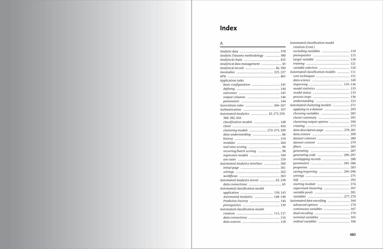
483

Index

A

Analytic data ........................................................... 378

Analytic Datasets methodology ..................... 380

Analytical chain ..................................................... 425

Analytical data management .............................. 45

Analytical record ............................................ 46, 390

Anomalies ...................................................... 225, 227

APIs ............................................................................. 465

Application tasks

basic configuration ......................................... 145

defining ................................................................ 144

outcomes ............................................................. 145

output columns ................................................ 146

parameters ......................................................... 144

Association rules ......................................... 266–267

Authentication ...................................................... 107

Automated Analytics ........................ 42, 173, 259,

368, 382, 416

classification models ...................................... 148

client ...................................................................... 456

clustering models .......................... 272–273, 299

data understanding ........................................... 86

history ................................................................... 150

modules ............................................................... 264

real-time scoring ................................................. 98

recurring/batch scoring ................................... 98

regression models ............................................ 184

use cases .............................................................. 259

Automated Analytics interface ....................... 260

initial page .......................................................... 261

settings ................................................................. 262

workflows ............................................................ 263

Automated Analytics server ...................... 65, 238

data connections ................................................. 65

Automated classification model

application ................................................ 139, 143

Automated Analytics ........................... 148–149

Predictive Factory ............................................ 144

prerequisites ....................................................... 139


creation ...................................................... 115, 117

data connections .............................................. 116

data sources ....................................................... 118


creation (Cont.)

excluding variables ......................................... 119

prerequisites ...................................................... 115

target variable .................................................. 118

training ................................................................ 121

variable selection ............................................. 120

Automated classification models .................. 111

core techniques ................................................. 151

data science ....................................................... 149

improving ................................................. 135–136

model statistics ................................................. 133

model status ...................................................... 133

process steps ...................................................... 136

understanding .................................................. 123

Automated clustering models ........................ 271

applying to a dataset ..................................... 293

choosing variables .......................................... 283

cluster summary .............................................. 291

clustering output options ............................. 294

creating ................................................................ 273

data description page ........................... 279, 281

data science ....................................................... 299

dataset columns ............................................... 280

dataset content ................................................ 279

filters ..................................................................... 283

generating .......................................................... 287

generating code ...................................... 296–297

overlapping records ........................................ 288

parameters ............................................... 285–286

properties ............................................................ 283

saving/exporting ................................... 295–296

settings ................................................................. 275

SQL ......................................................................... 292

starting module ................................................ 274

supervised clustering ...................................... 297

variable pools .................................................... 281

variables ..................................................... 277, 279

Automated data encoding ................................ 164

advanced options ............................................ 170

continuous variables ...................................... 167

dual encoding .................................................... 170

nominal variables ............................................ 165

ordinal variables .............................................. 166

Index

484

Automated data preparation ........................... 160

Automated engine ............................................... 152

Automated model creation ................................. 45

Automated Predictive Library ........ 74, 347, 374,

418, 451

functions ............................................................. 374

Automated Recommendation models ........ 347

Automated regression models ....................... 173

applying ..................................................... 184, 186

Automated Analytics ..................................... 190

creating ....................................................... 174, 176

dataset statistics .............................................. 182

datasets ............................................................... 174

improving ........................................................... 183

model statistics ................................................ 183

model status ...................................................... 182

parameters ......................................................... 177

performance indicators ................................ 183

predicted versus actual curve ..................... 180


understanding .................................................. 179

uniform target encoding .............................. 475

variable contributions ................................... 181

variable metadata ........................................... 178

Automated server ................................................ 252

Autoregressive approach .................................. 230

B

Batch production ..................................................... 45

Best practices ......................................................... 467

Best-sellers ..................................................... 349, 370

Binning ..................................................................... 164

Bipartite graphs ........................... 47, 305, 354, 359

creation ................................................................ 355

Bottlenecks ................................................................ 82

Business question ................................................ 382

Business representatives ............................... 32, 79

project requirements ......................................... 35

Business understanding phase ................... 79, 81

banking use case .......................................... 82–83

insurance use case .............................................. 85

management sponsers ..................................... 84

manufacturing use case .................................. 84

C

Centroids .................................................................. 299

Chi-squared tests ............................................ 44, 243

Classification models ...... 94, 111–112, 174, 452

applying ............................................................... 113

deployment ......................................................... 237

example ................................................................ 114

probability code ................................................ 453

Classification technique ..................................... 112

learning phase ................................................... 113

Cleaning policy ....................................................... 240

Cluster profiles ................................... 287, 289, 292

qualitative matrix ............................................ 290

supervised clustering ...................................... 298

Clustering ................................................................. 271

automated approach ...................................... 272

supervised ............................................................ 272

unsupervised ...................................................... 272

Clustering models .......................................... 95, 473

Colocation analysis .............................................. 340

colocations .......................................................... 344

geographical algorithm ................................. 343

parameters .......................................................... 342

time interval ....................................................... 343

Communities .......................................................... 302

community tree ................................................ 335

detecting .................................................... 316–317

identifiers ............................................................. 365

information ........................................................ 326

visualization ....................................................... 361

Composite variables ........................ 469, 471–472

polynomial degree ........................................... 473

predictions as predictors ............................... 473

Confidence ..................................................... 349, 373

Consistency ............................................................. 154

Contact graph ......................................................... 312

fields ............................................................. 312–313

Continuous variables ...................... 120, 277–278

Control ....................................................................... 104

Convergence speed .............................................. 154

CRISP-DM methodology ................. 23, 41, 77, 81

Cutting strategy ..................................................... 162

Cycles ......................................................................... 203

Cyclical patterns .................................................... 229

485

Index

D

Data analysts ...................................................... 33, 79

modeling phase ................................................... 94


Data Manager ...... 45, 47, 88, 106, 238, 246, 260,

264, 377, 464


create entity ....................................................... 384

create objects ..................................................... 383

deriving predictors .......................................... 469

edit time-stamped population ................... 386

improving predictive power ........................ 138

objects ................................................................... 408

transactional data ...................................... 89–90

Data manipulation ..................................... 378, 392

Data preparation ............................................ 45, 377

Data preparation phase .................................. 79, 87

data quality ........................................................... 92

database views ..................................................... 88

dates ......................................................................... 92

dynamic time concept ...................................... 90

reusing content .................................................... 92

SAP HANA .............................................................. 88

transactional data .............................................. 88

Data preview ........................................................... 403

Data quality ............................................................. 467

Data scientists ........................................................... 33

Data sets ................................................................... 267

Data sources ............................................................ 238

Data split .................................................................. 227

Data transfer .................................................... 47, 267

Data understanding phase ............................ 79, 85

Data Viewer ............................................................. 267

Data visualization .................................................... 48

Database schema .................................................. 392

Datasets .................................................................... 379

building ................................................................ 379

creation ................................................................ 381

Debriefing tables ................................................... 371

De-cycling ................................................................ 229

Density ...................................................................... 325

Deployment phase ........................................... 80, 97

Derived graphs ............................................. 354, 357

Descriptive statistics .............................................. 48

Detected curve .................................... 128–129, 158

De-trending ............................................................. 228

extra predictables ............................................ 228

Deviation probability ......................................... 142

Deviations ...................................................... 140, 241

prediction confidence .................................... 143

understanding .................................................. 142

Distinct values .......................................................... 48

Documentation ..................................................... 402

Domains ................................................................... 401

Dynamic time concept .......................................... 91

E

Encoding towards the target ............................ 467

Entity ........................................................... 46, 90, 381

Error matrix ............................................................ 129

metrics .................................................................. 130

Evaluation phase .............................................. 80, 96

predictive models ................................................ 96

Event log aggregation ......................................... 264

Event-based scheduling ..................................... 253

Excluded variables ............................................... 284

Expert Analytics ..................... 42, 95–96, 260, 415

automated approach ..................................... 415

data explorations ............................................ 420

data preparation ............................................. 422

data sources .............................................. 418, 420


data writer .......................................................... 423

graphical components ................................... 422

model deployment .......................................... 253

models .................................................................. 423

open-source language R ............................... 442

optimizations .................................................... 423


project workflow .............................................. 417

SAP Lumira ......................................................... 421

using R algorithms ............................................. 73

when to use ........................................................ 415

Expert Analytics algorithms ................... 422, 438

connected to SAP HANA ............................... 438

other connectivity types ............................... 440

Expert Analytics extended functionality ... 442

R Editor ................................................................ 442

R extensions ............................................. 445–447

R function ........................................................... 444

Index

486

Expert Analytics interface

executing node chains ................................... 417

navigating .......................................................... 416

Expert Analytics predictive models

analytical chain ................................................ 433

column mapping ............................................. 435

creating ....................................................... 427, 430

data exploration .............................................. 431

dataset columns ............................................... 428

loading data ...................................................... 428

model deployment .......................................... 436

model performance ........................................ 434

partition node ................................................... 432

Explanatory variables ......................................... 284

Exploratory analytics ............................... 27, 29–30

business case ........................................................ 35

Exporting models ................................................. 451

External executables ........................................... 107

External task ........................................................... 108

Extra predictables ...................................... 210–211

cycles ..................................................................... 229

MAPE .................................................................... 212

missing values .................................................. 211

F

Filtered line count ................................................ 325

Filters ................................................................ 386, 399

Flat files .................................................................... 196

Fluctuations ................................................... 195, 203

time series forecasts ....................................... 230

Forecasts ......................................................... 210, 218

Formula Editor ...................................................... 398

Frequent path analysis .............................. 340, 344

Future target period ............................................... 90

G

Gain charts ..................................................... 149, 190

Generalization capacity control ..................... 155

Graph comparison ............................................... 335

Graph theory ............................................................. 47

Graphical workbench .......................................... 416

Graphs ....................................................................... 348

I

Industry use cases ................................................... 37

automotive or high tech .................................. 39

banks and financial institutions .................. 38

consumer goods .................................................. 38

retail ........................................................................ 38

Telecom .................................................................. 37

Integration ............................................................... 451

in-database ......................................................... 455

Intra-community members ............................. 363

IT experts .................................................................... 79

IT team ......................................................................... 33


J

Joins .............................................................................. 46

K

Keycode ..................................................................... 263

K-Means algorithm ............................................... 299

KXEN .......................................................................... 150

KxScript ..................................................................... 475

KxShell engine ....................................................... 464

KxShell Script ......................................... 98, 107, 458

L

Linear in extra predictables .............................. 228

Linear regression ................................................... 174

Linear trend ............................................................. 204

Link analysis .............................................................. 47

Links ................................................................. 302, 348

directed ................................................................. 302

undirected ........................................................... 302

weight ................................................................... 302

Lorenz Curve ........................................................... 133

Louvain algorithm ................................................ 316

M

Machine-to-machine solutions ......................... 29

MAPE value .......................................... 202, 230–231

Massive predictive analytics ............................ 233

487

Index

Massive tasks

scheduling ........................................................... 250

Mega-hubs ..................................................... 303, 317

detecting .............................................................. 317

Merging tables ....................................................... 391

Metadata .................................................................. 408

Metadata repository ............................................ 238

Missing values ....................................................... 161

Model accuracy ...................................................... 210

Model building ......................................................... 43

Model control ............................................................ 43

Model deviation ....................................................... 44

Model deviation test task .................................. 242

creating ................................................................ 140

outputs ................................................................. 242

results ................................................................... 142

running ................................................................ 141

Model maintenance ................................................ 99

Model quality ......................................................... 241

Model repository .................................................. 234

Model retraining .................................. 44, 104, 244

maximum global performance loss ......... 247

outputs ................................................................. 247

parameters ......................................................... 245

tasks ...................................................................... 244

Model settings ....................................................... 464

Model training ...................................... 42, 369, 464

Model training delegation ................................ 261

Modeling phase ................................................. 80, 93

Automated Analytics ........................................ 94

machine learning functionalities ................. 94

Predictive Factory ............................................... 93

Modeling server .......................................... 106, 116

Modularity ............................................................... 326

Multicollinearity ................................................... 161

N

Nearest neighbors graph ................................... 312

Node display ........................................ 328, 359, 371

Node pairing ................................................. 304, 335

SNA model ................................................ 318–319

Nodes ............................................................... 302, 348

attributes ............................................................. 303

degree ................................................................... 302

neighbors ............................................................. 302

Nodes (Cont.)

partition node ................................................... 422

roles ....................................................................... 303

social pressure ................................................... 302

source node ........................................................ 302

target .................................................................... 302

Nominal variables ....................................... 120, 277

Number of records ............................................... 162

O

ODBC ......................................................................... 378

Optimized groups ......................................... 48, 268

Ordinal variable .................................................... 120

Outliers ..................................................................... 162

Output columns .................................................... 188

Output table ........................................................... 240

Overfitting ............................................................... 152

P

Parameter trees ..................................................... 456

Past target period .................................................... 91

Path analysis ........................................................... 306

Performance curves ............................................ 132

Piecewise continuous encoding ..................... 168

Polynomial degree ............................................... 473

Prediction confidence ............ 124, 136, 243, 435

improving ........................................................... 137

regression models ................................... 180, 184

Predictive Analysis Library (PAL) ..... 43, 75, 418

Predictive analytics projects ........................ 32, 78

business case ........................................................ 34

execution and lifecycle management ........ 36

planning ................................................................. 77

requirements ........................................................ 35

running a project ................................................ 81

stakeholders .......................................................... 32

Predictive Factory ................... 37, 43–44, 49, 103,

173, 199, 203, 237, 254, 260

authentication ..................................................... 68

automated regression models .................... 176

automated server ............................................... 63

classification models ............................. 115, 123

clustering models ............................................. 295

communication ................................................... 68

Index

488

Predictive Factory (Cont.)

defining users ....................................................... 68

downloading ........................................................ 61

end-to-end modeling ...................................... 103

external commands ........................................... 71

in-app help ............................................................ 70

installing ......................................................... 61–62

license ...................................................................... 63

model maintenance ........................................... 99

post-installation ................................................. 63

project .................................................................. 105

recurring/batch scoring ................................... 98

restarting ............................................................... 71

SAP HANA server ................................................ 66

system requirements ......................................... 61

Predictive Modeling Markup Language

(PMML) ................................................................ 426

Predictive models ................................... 26, 41, 112

adding data rows ............................................. 474

adding predictors ............................................ 468

batch mode ........................................................ 234

data description ............................................... 468

improving quality ............................................ 467

mass production ................................................. 45

modeling process ................................................ 93

segmented modeling ...................................... 475

Predictive pipeline ............................................... 254

Predictive power ..................... 123–124, 136, 243,

349, 435, 468

improving ................................................. 137–138

indicating ............................................................ 159

regression models ................................... 180, 184

Prescriptive analytics ...................................... 25, 28

decision factors ................................................... 31

model ....................................................................... 28

Probability calculation ....................................... 454

Product Availability Matrix (PAM) ....... 453, 476

Product documentation .................................... 476

Profit simulation ........................................ 131–132

Project creation ..................................................... 105

Project lead ................................................................ 33

Prompts .................................................................... 406

Proximity graph ................................................... 312

R

R environment ....................................................... 442

R extension .................................................... 445, 448

R logic ......................................................................... 448

R server ............................................................... 75, 418

R syntax .................................................................... 444

Real-time scoring .................................................... 98

Recommendation models ......... 47, 95, 363, 371

approaches .......................................................... 351

details .................................................................... 358

SNA ......................................................................... 353

Recommendation module ................................ 368

create model ....................................................... 368

Recommended products .................................... 366

Recurring cycles ..................................................... 195

Recurring forecasts ............................................... 222

active schedule .................................................. 225

monitoring .......................................................... 226

schedule interval ............................................... 224

Recurring/batch scoring ...................................... 98

Reference date .......................................................... 46

Regression models ..................... 95, 173–174, 184

deployment ......................................................... 237

Relationships .......................................................... 360

Reports ...................................................................... 243

abnormally connected nodes ...................... 328

communities size distribution .................... 328

nodes degree distribution ............................. 328

nodes with highest degree ............................ 328

Residuals ......................................................... 195, 210

Result production ................................................. 104

Ridge regressions .................................................. 157

RStudio Desktop .................................................... 442

S

SAP Analytics Cloud ............................................... 30

SAP Community for SAP Predictive

Analytics .............................................................. 476

SAP Data Services .................................................. 468

SAP HANA server ............................................ 66, 234

setting up ............................................................... 67

SAP HANA smart data streaming ................... 453

SAP HANA Studio .................................................. 438

SAP HANA views .................................................... 238

489

Index

SAP JVM ....................................................................... 59

SAP Lumira .......................................................... 30, 48

SAP Notes ................................................................. 478

SAP Predictive Analytics ............... 26–27, 41, 301

additional resources ....................................... 476


benefits .................................................................... 29

composite variables ........................................ 469


deployment phase .............................................. 97

expert analytics models ................................... 50

exploratory analytics ........................................ 30

goals ...................................................................... 149

installing ................................................................. 49

recommended deployments ........................... 50

regression models ............................................ 174

scripting ............................................................... 456

SAP Predictive Analytics client ................ 49, 259

checking installation ......................................... 60

downloading ......................................................... 58

installing .......................................................... 57, 59

Linux ........................................................................ 60


SAP Predictive Analytics desktop ............ 49, 259

installing ......................................................... 71–72

post-installation .................................................. 73


SAP Predictive Analytics license ........................ 55

Linux installation ............................................... 56

Windows installation ........................................ 55

SAP Predictive Analytics server ......................... 49

downloading ......................................................... 51

installing .......................................................... 51, 53

Linux ........................................................................ 54

Microsoft Windows ............................................ 53

post-installation .................................................. 54

post-installation steps ...................................... 56

SAP Support Portal .................................................. 50

SAP’s App Center ................................................... 442

Scheduling ..................................................... 236, 251

Score calculation ................................................... 454

Scorecards ................................................................ 453

Seasons ..................................................................... 229

Segmented modeling .......................................... 139

Sensitivity curve ................................................... 132

Sequence analysis ................................................. 264

industry use case ................................................. 38

Simple model indicators ................................... 158

Snapshot datasets ................................................ 379

Social graph ............................................................. 302

Social model ........................................................... 365

Social Network Analysis ....................... 47, 95, 353

adding graphs ................................................... 314

automated functionality .............................. 303

bipartite graphs derivation ......................... 305

communities and roles detection .............. 304

creating ...................................................... 306–307

defining graphs ...................................... 310–312

describing nodes .............................................. 320

descriptive attributes ..................................... 321

identifiers conversion ..................................... 320

importing dataset ................................. 308–309

modeling parameters ..................................... 322

naming conventions ............................ 338–339

node pairing ....................................................... 304

path analysis ..................................................... 306

Proximity module ............................................ 305

Recommendations module .......................... 305

social graph comparison .............................. 305

terminology ....................................................... 302

Social Network Analysis output ..................... 323

analyzing communities ................................ 334

application dataset ......................................... 337

applying the model ......................................... 336

commands ................................................ 331–332

customizing nodes .......................................... 332

dataset output location ................................ 339

generation optins ............................................ 337

generation options .......................................... 337

graphs ................................................................... 325

model overview ...................................... 323–324

navigating .......................................................... 328

node navigation ............................................... 329

organizing nodes ............................................. 333

reports .................................................................. 327

SQL code ................................ 46, 373, 378, 406, 452

SQL settings ............................................................ 411

SQL syntax .................................................................. 98

Standard encoding ............................................... 166

Standardization encoding ................................ 168

Statistical Learning Theory ............................... 154

variables .............................................................. 160

Index

490

Stored procedure in SAP HANA ...................... 426

Stratified sampling .............................................. 388

Structural risk minimization (SRM) ..... 152, 155

benefits ................................................................ 160

Supervised clustering ......................................... 297

Support ..................................................................... 349

T

Target mean ............................................................ 165

Target mean encoding ....................................... 166

Target periods ........................................................... 91

Target statistics ..................................................... 128

Target variable ................................................ 90, 284


Targeted clustering .............................................. 473

Temporal aggregates ........................................... 394

period settings .................................................. 395

Text analysis ........................................................... 264

Textual variable .................................................... 120

Third-party code ................................................... 451

Third-party vendors ............................................ 465

Time interval .......................................................... 236

Time series .............................................................. 193

Time series datasets ............................................ 380

Time series forecasting mass production

applying models ............................................... 221

MAPEs .................................................................. 217

metadata ............................................................ 216

settings ................................................................. 216

trained model .................................................... 217

warnings ............................................................. 220

Time series forecasting models ............... 95, 193

accuracy .............................................................. 210


creating ................................................................ 195

creating a project ............................................. 197

data connection ............................................... 197

data science ....................................................... 227

dates ...................................................................... 200

deployment task .............................................. 235

extra predictables ............................................ 211

forecasted values .................................... 204, 209

history .................................................................. 202

importing ............................................................ 234

Time series forecasting models (Cont.)

improved forecasts .......................................... 213

missing values ................................................... 196

model report ....................................................... 203

outliers .................................................................. 204

output columns ................................................. 209

productizing ....................................................... 221

reducing history ................................................ 474

SAP HANA table ................................................ 208

saving .................................................................... 206

trained model .................................................... 202

understanding ................................................... 202

use case ................................................................. 194

variable types ..................................................... 200

Time-stamp ............................................................. 379

Time-stamped population ............... 46, 381, 386

complex ................................................................ 389

Toolkit module ....................................................... 266

options .................................................................. 267

Trained model ........................................................ 424

Training dataset ....................................................... 43

Transaction datasets ............................................ 380

Transactional relationships .............................. 301

Transactions graph ........................... 312, 354, 356

Trend over time ..................................................... 195

Trends ........................................................................ 203

Triple exponential smoothing ......................... 230

U

Underfitting ............................................................ 152

Union ............................................................... 389, 474

V

Validation curve .................................................... 180

Vapnik’s principles ............................................... 156

Vapnik-Chervonenkis theory ........................... 153

Variable contributions .............................. 125, 181

Variable statistics .................................................. 110

Variable structures ............................................... 171

VC dimension ............................................... 154–155

Predictive Factory and Automated

Analytics ......................................................... 157

Visibility .................................................................... 400

491

Index

W

Weight ....................................................................... 348

Weight variables .................................................... 284

Wildcards ................................................................. 399

Windows Active Directory (Kerberos) ............. 68

Wizard curve ........................................................... 180

Working directory ................................................ 107

First-hand knowledge.

We hope you have enjoyed this reading sample. You may recommend or pass it on to others, but only in its entirety, including all pages. This reading sample and all its parts are protected by copyright law. All usage and exploitation rights are reserved by the author and the publisher.

Antoine Chabert is a product manager for SAP Predictive Analytics. He joined SAP in 2007 as a product owner for SAP BusinessObjects, where he work was dedicated to the semantic layer.

Andreas Forster is a member of SAP‘s Global Center of Excellence for Analytics, based in Switzerland. In his current role, he focuses on scaling the SAP Predictive Analytics organization through enablement, business development, and strategic deal support.

Laurent Tessier is a predictive analytics expert at the Global Center of Excellence for SAP Predictive Analytics. His work encompasses all phases of the sales cycle, from posi-tioning presentations and discovery workshops to scoping and project execution.

Antoine Chabert, Andreas Forster, Laurent Tessier, Pierpaolo Vezzosi

SAP Predictive Analytics: The Comprehensive Guide491 Pages, 2018, $79.95 ISBN 978-1-4932-1592-8

www.sap-press.com/4491

Pierpaolo Vezzosi is director of product management in the SAP Analytics organization. He is currently working on analytics on big data, semantics, Web Intelligence and SAP Leonardo.

https://www.sap-press.com/sap-predictive-analytics_4491/authors/?utm_source=AWS&utm_medium=readingsample&utm_campaign=Browse%20the%20Book&utm_content=1592

sap predictive analytics: the comprehensive guide · pdf filereading sample this sample...

Documents