r/v mirai cruise report mr12-03 · 2014-09-29 · at first, engine trouble during this cruise...

R/V Mirai Cruise Report MR12-03

July 17, 2012 – August 29, 2012

Tropical Ocean Climate Study (TOCS)

Japan Agency for Marine-Earth Science and Technology (JAMSTEC)

Table of contents

1. Cruise name and code 1-1 2. Introduction and observation summary 2-1

2.1 Introduction 2-1 2.2 Overview 2-2 2.3 Observation summary 2-2 2.4 Observed oceanic and atmospheric conditions 2-4

3. Period, ports of call, cruise log and cruise track 3-1 3.1 Period 3-1 3.2 Ports of call 3-1 3.3 Cruise log 3-1 3.4 Cruise track 3-14

4. Chief scientist 4-1 5. Participants list 5-1

5.1 R/V MIRAI scientists and technical staffs 5-1 5.2 R/V MIRAI crew members 5-2

6. General observations 6-1

6.1 Meteorological measurements 6-1 6.1.1 Surface meteorological observations 6-1 6.1.2 Ceilometer 6-10

6.2 CTD/XCTD 6-14 6.2.1 CTD 6-14 6.2.2 XCTD 6-31

6.3 Water sampling 6-36 6.3.1 Salinity 6-36

6.4 Continuous monitoring of surface seawater 6-41 6.4.1 Temperature, salinity and dissolved oxygen 6-41 6.5 Underway pCO2 6-45 6.6 Shipboard ADCP 6-47 6.7 Underway geophysics 6-51

6.7.1 Sea surface gravity 6-51 6.7.2 Sea surface magnetic field 6-53 6.7.3 Swath bathymetry 6-55

7. Special observations 7-1

7.1 TRITON buoys 7-1 7.1.1 Operation of the TRITON buoys 7-1 7.1.2 Inter-comparison between shipboard CTD and TRITON 7-7

transmitted data 7.1.3 Performance test of pCO2 sensor 7-11

7.2 Subsurface ADCP moorings 7-13

7.3 Current profile observations using a high frequency lowered 7-21 acoustic Doppler current profiler

7.4 Observation of ocean turbulence 7-27 7.5 Argo floats 7-33 7.5.1 Profiling floats for JAMSTEC Argo Project 7-33

7.5.2 ARGO float mission off Papua New Guinea 7-35 7.6 Global Drifter Program – SVP Drifting Buoys 7-38 7.7 Radiosonde observation for the validation of GOSAT and ship-borne 7-40

sky radiometer products 7.8 Validation of GOSAT products over sea using a ship-borne compact 7-44

system for measuring atmospheric trace gas column densities 7.9 Lidar observations of clouds and aerosol 7-47 7.10 Aerosol optical characteristics measured by Shipborne 7-49

Sky radiometer 7.11 Continuous measurement of the water stable isotopes 7-50

over the Ocean 7.12 Rock sampling using a dredge 7-55

Note:

This cruise report is a preliminary documentation as of the end of the cruise. It

may not be revised even if new findings and others are derived from observation

results after publication. It may also be changed without notice. Data on the cruise

report may be raw or not processed. Please ask the chief scientist for the latest

information before using this report. Users of data or results of this cruise are

requested to submit their results to Data Integration and Analysis Group (DIAG),

JAMSTEC (e-mail: [email protected]).

1-1

1. Cruise name and code

Tropical Ocean Climate Study

MR12-03

Ship: R/V Mirai

Captain: Yasushi Ishioka

2-1

2. Introduction and observation summary

2.1 Introduction The purpose of this cruise is to observe ocean and atmosphere in the western tropical Pacific

Ocean for better understanding of climate variability involving the ENSO (El Nino/Southern

Oscillation) phenomena. Particularly, warm water pool (WWP) in the western tropical Pacific is

characterized by the highest sea surface temperature in the world, and plays a major role in driving

global atmospheric circulation. Zonal migration of the WWP is associated with El Nino and La Nina

which cause drastic climate changes in the world such as 1997-98 El Nino and 1999 La Nina.

However, this atmospheric and oceanic system is so complicated that we still do not have enough

knowledge about it.

In order to understand the mechanism of the atmospheric and oceanic system, its high quality

data for long period is needed. Considering this background, we developed the TRITON (TRIangle

Trans-Ocean buoy Network) buoys and have deployed them in the western equatorial Pacific and

eastern Indian Ocean since 1998 cooperating with USA, Indonesia, and India. The major mission of

this cruise is to maintain the network of TRITON buoys along 147E and 156E lines in the western

equatorial Pacific.

During this cruise, we observe the low-latitude western boundary currents in the South Pacific

contributing to the SPICE (Southwest Pacific Ocean Circulation and Climate Experiment) project,

which was endorsed by CLIVAR in 2008. We conduct observations in the area of north of New

Ireland of Papua New Guinea because we focus the New Ireland Coastal Undercurrent (NICU),

where observation data is very limited. For this purpose, two subsurface Acoustic Doppler Current

Profiler (ADCP) buoys are deployed and one Argo float is launched near the northern coast of New

Ireland. Additionally, XCTD and shipboard ADCP observations are conducted in the Papua New

Guinea EEZ/territorial water.

We have been observed ocean fine structure in order to understand ocean mixing effect on

tropical ocean climate since MR07-07 leg 1 collaborating with International Pacific Research Center

(IPRC) of USA. For this purpose, we conducted CTD observations with a Lowered ADCP (LADCP)

and ocean turbulence observations along 147E and 156E lines.

During this cruise, 20 surface drifters, which were prepared by Atlantic Oceanographic and

Atmospheric Laboratory (AOML) of National Oceanic and Atmospheric Administration (NOAA),

are deployed for contribution to the global observational network along 156E between 5S and 14N.

Radiosonde observations were conducted in the Kuroshio Extension region and Tropical region

for understanding air-sea interaction in the Kuroshio Extension, and getting support data for CO2

measurement.

North of Papua New Guinea is also interesting area in geophysics. Particularly, the Early

Cretaceous Ontong Java Plateau and neighboring ocean basin flood basalts in the western Pacific

constitute the most voluminous Large Igneous Province on the Earth. For further better

2-2

understanding of mechanism of generation of Ontong Java Pleatau, bottom igneous rocks and

sediments on the ocean bottom are sampled using a dredge near the Nuugurigia Island (4-16S,

157-23E) during this cruise.

Except for above, automatic continuous oceanic, meteorological and geophysical observations

are also conducted along ship track during this cruise as usual. In particular, a cesium magnetometer

is towed in the Lyra Basin (Between 147E and 156E) and near the dredge points.

2.2 Overview

1) Ship

R/V Mirai

Captain Yasushi Ishioka

2) Cruise code

MR12-03

3) Project name

Tropical Ocean Climate Study (TOCS)

4) Undertaking institution

Japan: Japan Agency for Marine-Earth Science and Technology (JAMSTEC)

2-15, Natsushima-cho, Yokosuka, 237-0061, Japan

5) Chief scientist

Chief Scientist (Japan)

Yuji Kashino, Japan Agency for Marine-Earth Science and Technology (JAMSTEC)

6) Period

July 17, 2012 (Sekinehama, Japan) – August 29, 2012 (Sekinehama, Japan)

7) Research participants

Seven scientists, one engineer, and twenty marine technicians from Japanese

Institutes/University/Companies

. 2.3 Observation summary TRITON buoy recovery and re-installation: 9 moorings were deployed and

9 moorings were recovered.

Subsurface ADCP moorings: 3 moorings were deployed and

2-3

2 moorings were recovered

CTD (Conductivity, Temperature and Depth) and water sampling: 43 casts

XCTD: 36 casts

Ocean turbulence observation 78 casts

Launch of Argo floats 2 floats

Launch of surface drifters 20 drifters

Radiosonde 45 casts

Rain and surface water sampling for isotope analysis

37 casts for rain and 43 casts for surface water

Current measurements by shipboard ADCP: continuous

Sea surface temperature, salinity, and dissolved oxygen,

measurements by intake method: continuous

CO2 measurement continuous

Surface meteorology: continuous

Water vapor observation: continuous

Underway geophysics observations continuous

Towing a cesium magnetometer and sub-bottom profiler observations continuous, 3 times

Rock sampling using a dredge 6 times

At first, engine trouble during this cruise should be noted; one of four engines of R/V Mirai did

not work from 25 July to 21 August. and cruise speed reduced to 11 knot during this period. Because

of this trouble, we should save ship time and canceled four casts of CTD/ocean turbulence

observations between 2.5N and 4N along 147E. Except for these cancel, we conducted all planed

observations. Engine was repaired on 21 August.

We recovered and re-installed nine TRITON buoys along 147E and 156E lines during this

cruise. Among of them, TRTION buoy #4 started drifting on 28 may 2012, and its float and

underwater sensors until 150m depth were recovered by Korean Research Vessel, R/V Onnuri, on 28

June. We found underwater parts of this buoy below 175m on 11 August using acoustic instrument,

and recover them on 12 August. Unfortunately, we found that the ADCP installed at the depth of

175m was lost. We did not find severe damages of buoys except for the TRITON buoy #4.

We also successfully recovered and deployed subsurface ADCP buoys. However, data from the

ADCPs could not be downloaded. Battery of the ADCP was exhausted when they were recovered

because mooring period was extended to 1.5 years although parameters of ADCP were for one-year

mooring. From this cruise, we changed ADCP parameters for 1.5-years mooring (the number of

pings of ADCP per unit time was reduced).

During this cruise, we conducted shallow CTD casts with a LADCP until 500m or 800m depth

and ocean turbulence observation using a Microstructure Profiler (MSP), Turbo-Map L, along 147E

and 156 lines. Additionally, we conduct following special observations using CTD/LADCP and

2-4

MSP for better understanding of ocean fine structure and its time variability:

(a) Observations with meridional interval of 15 nautical miles between 2N and equator along

156E. Each station consists of a CTD/LADCP cast to 500m depth followed by 3 MSP casts. .

(b) A 24-hour station at the equator, 156E with a CTD/LADCP cast every 3hrs with 3 MSP casts in between.

We deployed two Argo floats during this cruise. One was aimed to construct the global ocean

dataset under Japan Argo Project. The other was deployed for measuring temperature/salinity

profiles in the NICU region. Unfortunately, data communication from the latter float was stopped

after sending data of only one profile. We need to check its reason after this cruise.

As shown in 2.1, we carried out rock sampling using a dredge from 6 August to 8 August.

During this period, towing of dredge was carried out 6 times around 4-16S, 157-23E on the flanks of

the three sea mount. Although fuse wire of the dredge was cut two times, rocks and dredge were

successfully recovered.

All automatic continuous meteorological, oceanographic and geophysical observations were

carried out well.

Thus, we conducted all planed observations on schedule in this cruise except for cancel of four

CTD/LADCP and MSP casts along 147E in spite of the engine trouble of R/V Mirai.

2.4 Observed oceanic and atmospheric conditions In 2012 boreal summer, atmosphere and ocean in the tropical Pacific was under the normal

condition. Japan Meteorological Agency suggested possibility of occurrence of El Nino after this

summer. Because of this condition, sea surface temperature (SST) anomaly was higher than 1 degree

in the whole equatorial Pacific, and westerly wind was observed west of 156E (Figure. 2-1).

During this cruise, sea state was good and suitable for buoy maintenance work in spite of many

rainy/cloudy days, which were associating with weak Maddan Julian Oscillation. Surface salinity

was low because of this condition (Figure 2-2).

2-5

Figure 2-1. Maps of sea surface temperature and winds (upper panel), and their anomaly (lower panel)

obtained from TAO/TRITON buoy array on 5 August 2012. (http://www.pmel.noaa.gov/tao/jsdisplay/)

Figure 2-2. Temperature, salinity and potential density sections along 156E line.

3-1

3. Period, ports of call, cruise log and cruise track 3.1 Period

17th July 2012 – 29th August 2012

3.2 Ports of call Sekinehama, Japan (Departure: 17th July 2012) Sekinehama, Japan (Arrival: 29th August 2012)

3.3 Cruise Log

SMT UTC Event Jul. 17th (Tue.) 2012

08:50 23:50 (-1day) Departure of Sekinehama [Ship Mean Time (SMT)=UTC+9h] 10:30 01:30 Safety guidance 11:00 02:00 Surface sea water sampling start 13:15 04:15 Emergency drill 15:00 06:00 Observation Meeting 16:45 07:45 Konpira ceremony

Jul. 18th (Wed.) 2012 05:34 20:34 Radiosonde observation (#1) 11:34 02:34 Radiosonde observation (#2) 17:31 08:31 Radiosonde observation (#3) 23:31 14:31 Radiosonde observation (#4)

Jul. 19th (Thu.) 2012 05:31 20:31 Radiosonde observation (#5)

Jul. 20th (Fri.) 2012 12:00 03:00 Radiosonde observation (#6) 12:07 – 12:30 03:07 – 03:30 CO2 Observation (#1)

Jul. 21st (Sat.) 2012 23:10 14:10 Radiosonde observation (#7)

Jul. 23rd (Mon.) 2012 12:10 03:10 Radiosonde observation (#8) 12:11 – 12:40 03:11 – 03:40 CO2 observation (#2)

Jul. 24th (Tue.) 2012 22:00 13:00 Time adjustment +1h (SMT=UTC+10h)

Jul. 25th (Wed.) 2012 00:25 14:25 Radiosonde observation (#9) 10:00 00:00 Arrival at St. 1 (TR#7; 05-00N, 147-00E)

3-2

SMT UTC Event 12:42 02:42 Radiosonde observation (#10) 12:42 – 13:12 02:42 – 03:12 CO2 observation (#3) 13:06 –15:46 03:06 – 15:46 Deployment of TRITON buoy TR#7 (#1) (Fixed Position: 04-57.8151N, 147-01.6231E) 16:49 06:49 XCTD observation X-01 (#1) 18:03 – 18:41 08:03 – 08:41 CTD dC01M01 (800m) 18:44 – 19:17 08:44 – 09:17 MSP observation (#1) 19:17 – 19:47 09:17 – 09:47 MSP observation (#2)

Jul. 26th (Thu.) 2012 07:57 – 11:20 21:57 – 01:20 Recovery of TRITON buoy TR#7 (#1) 11:24 01:24 Departure of St. 1 14:42 04:42 Arrival at St. 2 (04-30N, 147-00E) 14:45 – 15:13 04:45 – 05:13 CTD dC02M01 (500m) 15:17 – 15:54 05:17 – 05:54 MSP observation (#3) 15:54 05:54 Departure of St. 2 18:42 08:42 XCTD observation X-02 (#2) 21:21 11:21 XCTD observation X-03 (#3)

Jul. 27th (Fri.) 2012 00:03 14:03 XCTD observation X-04 (#4) 02:40 16:40 XCTD observation X-05 (#5) 05:18 19:18 Arrival at St. 3 (TR#8; 02-00N, 147-00E) 05:30 – 06:11 19:30 – 20:11 CTD dC03M01 (800m; near the TR#8 Recovery point) 06:16 – 06:54 20:16 – 20:54 MSP observation (#4) 08:04 – 11:35 22:04 – 01:35 Recovery of TRITON buoy TR#8 (#2) 11:36 01:36 Departure of St. 3 14:42 04:42 Arrival at St. 4 (01-30N, 147-00E) 14:45 – 15:13 04:45 – 05:13 CTD dC04M01 (500m) 15:17 – 15:55 05:17 – 05:55 MSP observation (#5) 16:00 06:00 Departure of St. 4 18:36 08:36 Arrival at St. 5 (01-00N, 147-00E) 18:40 – 19:09 08:40 – 09:09 CTD dC05M01 (500m) 19:15 – 19:54 09:15 – 09:54 MSP observation (#6) 20:00 10:00 Departure of St. 5

Jul. 28th (Sat.) 2012 00:05 14:25 Radiosonde observation (#11) 04:48 18:48 Arrival at St. 3 (TR#8; 02-00N, 147-00E) 05:07 – 05:30 19:07 – 19:30 Figure-8 turn for Three-components magnetometer calibration

(02-04.9N, 146-59.6E, #1)

3-3

SMT UTC Event 08:06 –11:00 22:06 – 01:00 Deployment of TRITON buoy TR#8 (#2) (Fixed Position: 02-04.4521N, 146-57.1186E) 12:40 02:40 Radiosonde observation (#12) 13:35 03:35 XCTD observation X-06 (#6) 13:36 03:36 Departure of St. 3

Jul. 29th (Sun.) 2012 05:12 19:12 Arrival at St. 7 (TR#9; EQ, 147-00E) 08:05 –10:29 22:05 – 00:29 Deployment of TRITON buoy TR#9 (#3) (Fixed Position: 00-03.5409N, 147-00.6787E) 11:18 01:18 XCTD observation X-07 (#7) 12:59 – 14:53 02:59 – 04:53 Recovery of ADCP buoy (#1) 16:12 06:12 Departure of St. 7 18:30 08:30 Arrival at St. 6 (00-30N, 147-00E) 18:35 – 19:06 08:35 – 09:06 CTD dC06M01 (500m) 19:10 – 19:45 09:10 – 09:45 MSP observation (#7) 19:48 09:48 Departure of St. 6

Jul. 30th (Mon.) 2012 02:00 16:00 Arrival at St. 7 (TR#9; EQ, 147-00E) 05:14 – 05:58 19:14 – 19:58 CTD dC07M01 (1000m; near the TR#9 Recovery point) 06:04 – 06:38 20:04 – 20:38 MSP observation (#8) 07:57 – 11:06 21:57 – 01:06 Recovery of TRITON buoy TR#9 (#3) 11:38 01:38 Departure of St. 7 11:23 01:23 Start of Cesium magnetometer observation (#1) 13:02 03:02 Suspend of Cesium magnetometer observation 13:44 03:44 Re-start of Cesium magnetometer observation

Jul. 31st (Tue.) 2012 00:25 14:25 Radiosonde observation (#13) 12:40 02:25 Radiosonde observation (#14) 12:40 – 13:10 02:40 – 03:10 CO2 observation (#4) 22:00 12:00 Time adjustment +1h (SMT=UTC+11h)

Aug. 1st (Wed.) 2012 05:56 18:56 End of Cesium magnetometer observation (#1) 09:11 22:11 XCTD observation X-08 (#8) 11:05 00:05 XCTD observation X-09 (#9) 11:48 00:48 Arrival at St. ADCP#1 (02-38.1S, 153-20.1E) 12:58 – 14:16 01:58 – 03:16 Deployment of ADCP buoy (#1) (Fixed Position: 02-38.1725S, 153-21.0438E) 14:54 03:54 Departure of St. ADCP#1 15:36 04:36 Arrival at St.8 (02-43.2S, 153-16.65E)

3-4

SMT UTC Event 15:40 – 16:24 04:40 – 05:24 CTD dC08M01 (1000m) 16:29 05:29 Deployment of Argo float (#1) 16:30 05:30 Departure of St. 8 17:04 06:04 XCTD observation X-10 (#10) 18:48 07:48 XCTD observation X-11 (#11) 20:43 09:43 XCTD observation X-12 (#12) 22:38 11:38 XCTD observation X-13 (#13)

Aug. 2nd (Thu.) 2012 04:12 17:12 Arrival at St. ADCP#2 (2-48.3S, 153-13.2E) 07:57 – 09:21 20:57 – 22:21 Deployment of ADCP buoy (#2) (Fixed Position: 02-48.3474S, 153-13.1757E) 10:00 23:00 Departure of St. ADCP#2 13:11 02:11 Radiosonde observation (#15) 13:11 – 13:41 02:11 – 02:41 CO2 observation (#5) 16:03 05:03 XCTD observation X-14 (#14) 18:08 07:07 XCTD observation X-15 (#15) 20:18 09:18 XCTD observation X-16 (#16) 22:25 11:25 XCTD observation X-17 (#17)

Aug. 3rd (Fri.) 2012 00:18 13:18 XCTD observation X-18 (#18) 01:25 14:25 Radiosonde observation (#16) 02:19 15:19 XCTD observation X-19 (#19) 04:14 17:14 XCTD observation X-20 (#20) 06:00 19:00 XCTD observation X-21 (#21) 07:45 20:45 XCTD observation X-22 (#22) 09:27 22:27 XCTD observation X-23 (#23) 18:12 07:12 Arrival at St. 12 (03-30S, 156-00E) 18:17 – 18:52 07:17 – 07:52 CTD dC12M01 (500m) 18:56 – 19:32 07:56 – 08:32 MSP observation (#9) 19:36 08:36 Departure of St. 12

Aug. 4th (Sat.) 2012 05:18 18:18 Arrival at St. 9 (TR#6; 05-00S, 156-00E) 05:28 – 05:53 18:28 – 18:18 Figure-8 turn for Three-components magnetometer calibration

(05-01.6S, 156-01.0E, #2) 08:04 – 09:38 22:04 – 23:38 Deployment of TRITON buoy TR#6 (#4) (Fixed Position: 05-02.0108S, 156-01.5378E) 13:01 – 13:43 02:01 – 02:43 CTD dC09M01 (800m) 13:47 – 14:23 02:47 – 02:23 MSP observation (#10) 14:24 03:24 Departure of St. 9

3-5

SMT UTC Event 17:36 06:36 Arrival at St. 10 (04-30S, 156-00E) 17:39 – 18:07 06:39 – 07:07 CTD dC10M01 (500m) 18:10 – 18:46 07:10 – 07:46 MSP observation (#11) 18:48 07:48 Departure of St. 10 21:36 10:36 Arrival at St. 9 (TR#6; 05-00S, 156-00E) 21:37 10:37 XCTD observation X-24 (#24)

Aug. 5th (Sun.) 2012 07:56 – 10:26 20:56 – 00:26 Recovery of TRITON buoy TR#6 (#4) 10:33 00:33 Deployment of Drifter buoy (#1) 10:36 00:36 Departure of St. 9 13:12 02:12 Radiosonde observation (#17) 16:12 05:12 Arrival at St. 11 (04-00S, 156-00E) 16:17 – 16:49 05:17 – 05:49 CTD dC11M01 (500m) 16:49 – 17:25 05:49 – 06:25 MSP observation (#12) 17:28 06:28 Deployment of Drifter buoy (#2) 17:28 06:28 Start of OTJ site survey (MBES and Sub-bottom profiler) 17:30 06:30 Departure of St. 11 21:42 10:42 XCTD observation X-D1 (#25)

Aug. 6th (Mon.) 2012 01:25 14:25 Radiosonde observation (#18) 03:03 16:03 XCTD observation X-D2 (#26) 06:19 19:19 End of OTJ site survey (MBES and Sub-bottom profiler) 06:42 19:42 Arrival at St. Dredge (04-16S, 157-24E) 08:00 – 10:27 21:00 – 23:27 Dredge (#1) 12:54 – 15:22 01:54 – 04:22 Dredge (#2) 15:43 04:43 Start of Cesium magnetometer observation (#2) 15:54 04:54 Departure of St. Dredge 15:54 04:54 Start of OTJ site survey (MBES and Sub-bottom profiler) 19:04 08:04 XCTD observation X-D3 (#27)

Aug. 7th (Tue.) 2012 06:28 19:28 End of Cesium magnetometer observation (#2) 06:29 19:29 End of OTJ site survey (MBES and Sub-bottom profiler) 06:42 19:42 Arrival at St. Dredge 07:57 – 10:20 20:57 – 23:20 Dredge (#3) 12:54 – 15:32 01:54 – 04:32 Dredge (#4) 15:51 04:51 Start of Cesium magnetometer observation (#3) 15:54 04:54 Departure of St. Dredge 16:06 – 16:52 05:06 – 05:52 Figure-8 turn for Three-components magnetometer calibration

(04-16.0S, 157-26.3E, #3)

3-6

SMT UTC Event 16:56 05:56 Start of OTJ site survey (MBES and Sub-bottom profiler)

Aug. 8th (Wed.) 2012 02:10 15:10 Radiosonde observation (#19) 06:29 19:29 End of OTJ site survey (MBES and Sub-bottom profiler) 06:30 19:30 End of Cesium magnetometer observation (#3) 07:00 20:00 Arrival at St. Dredge 07:56 – 10:27 20:56 – 23:27 Dredge (#5) 12:22 – 15:31 01:22 – 04:31 Dredge (#6) 13:10 02:10 Radiosonde observation (#20) 13:10 – 13:40 02:10 – 02:40 CO2 observation (#6) 15:36 04:36 Departure of St. Dredge 15:53 04:53 Start of OTJ site survey (MBES and Sub-bottom profiler)

Aug. 9th (Thu.) 2012 01:25 14:25 Radiosonde observation (#21) 05:30 18:30 Arrival at St. 15 (TR#9; 02-00S, 156-00E) End of OTJ site survey (MBES and Sub-bottom profiler) 05:35 – 06:18 18:35 – 19:18 CTD dC15M01 (800m) 06:21 – 06:59 19:21 – 19:59 MSP observation (#13) 07:57 – 10:36 20:57 – 00:36 Recovery of TRITON buoy TR#5 (#5) 10:42 23:42 Departure of St. 15 13:24 02:24 Arrival at St. 14 (02-30S, 156-00E) 13:28 – 13:56 02:28 – 02:56 CTD dC14M01 (500m) 14:02 – 14:36 03:02 – 03:36 MSP observation (#14) 14:36 03:36 Departure of St. 14 17:24 06:24 Arrival at St. 13 (03-00S, 156-00E) 17:26 – 17:55 06:26 – 06:55 CTD dC13M01 (500m) 17:58 – 18:33 06:58 – 07:33 MSP observation (#15) 18:50 – 19:22 07:50 – 08:22 MSP observation (#16) 19:25 08:25 Deployment of Drifter buoy (#3) 19:30 08:30 Departure of St. 14

Aug. 10th (Fri.) 2012 06:12 19:12 Arrival at St. 15 (TR#9; 02-00S, 156-00E) 08:05 – 10:04 21:05 – 23:04 Deployment of TRITON buoy TR#5 (#5) (Fixed Position: 02-01.0319S, 155-57.5176E) 12:25 01:25 Deployment of Drifter buoy (#3) 12:26 01:26 XCTD observation X-25 (#28) 12:30 01:30 Departure of St. 15 14:09 03:09 Radiosonde observation (#22) 15:24 04:24 Arrival at St. 16 (01-30S, 156-00E)

3-7

SMT UTC Event 15:25 – 15:56 04:25 – 04:56 CTD dC16M01 (500m) 16:01 – 16:35 05:01 – 05:35 MSP observation (#17) 16:36 05:36 Departure of St. 16 19:30 08:30 Arrival at St. 17 (01-00S, 156-00E) 19:32 – 20:02 08:32 – 09:02 CTD dC17M01 (500m) 20:05 – 20:42 09:05 – 09:42 MSP observation (#18) 20:51 09:51 Deployment of Drifter buoy (#3) 20:54 09:54 Departure of St. 17

Aug. 11th (Sat.) 2012 00:50 13:50 Radiosonde observation (#23) 05:30 18:30 Arrival at St. 19 (TR#4; EQ, 156-00E) 08:05 – 09:49 21:05 – 22:49 Deployment of TRITON buoy TR#4 (#6) (Fixed Position: 00-00.9741N, 156-02.4995E) 10:21 23:21 XCTD observation X-26 (#29) 11:10 00:10 Radiosonde observation (#24) 12:53 – 14:10 01:53 – 03:10 Recovery of ADCP buoy (#2) 13:10 02:10 Radiosonde observation (#25) 15:11 04:11 Radiosonde observation (#26) 15:38 – 16:01 04:38 – 05:01 Search for TRITON buoy TR#4 & SSBL Calibration (Fixed Position: 00-01.0636S, 155-57.3603E) 17:58 – 18:24 06:58 – 07:24 Figure-8 turn for Three-components magnetometer calibration

(00-03.2S, 155-58.6E, #4) Aug. 12th (Sun.) 2012

08:02 – 10:00 21:02 – 23:00 Recovery of TRITON buoy TR#4 (#6) 12:54 – 13:49 01:54 – 02:49 Deployment of ADCP buoy (#3) (Fixed Position: 00-02.2110S, 156-07.9543E) 14:10 03:10 Radiosonde observation (#27) 14:12 03:12 Departure of St. 19 17:18 06:18 Arrival at St. 18 (00-30S, 156-00E) 17:23 – 17:54 06:23 – 06:54 CTD dC18M01 (500m) 17:57 – 18:37 06:57 – 07:37 MSP observation (#19) 18:42 07:42 Departure of St. 18

Aug. 13th (Mon.) 2012 01:00 14:00 Arrival at St. 19 (TR#4; EQ, 156-00E) 02:30 15:30 Radiosonde observation (#28) 05:58 – 06:30 18:58 – 19:30 CTD dC19M01 (500m) 06:33 – 07:09 19:33 – 20:09 MSP observation (#20) 07:11 – 07:45 20:11 – 20:45 MSP observation (#21) 07:47 – 08:24 20:47 – 21:24 MSP observation (#22)

3-8

SMT UTC Event 08:58 – 09:27 21:58 – 22:27 CTD dC19M02 (500m) 09:31 – 10:05 22:31 – 23:05 MSP observation (#23) 10:06 – 10:38 23:06 – 23:38 MSP observation (#24) 10:39 – 11:16 23:39 – 00:16 MSP observation (#25) 11:56 – 12:23 00:56 – 01:23 CTD dC19M03 (500m) 12:26 – 13:03 01:26 – 02:03 MSP observation (#26) 13:05 – 13:37 02:05 – 02:37 MSP observation (#27) 13:40 – 14:25 02:40 – 03:25 MSP observation (#28) 14:56 – 15:23 03:56 – 04:23 CTD dC19M04 (500m) 15:27 – 16:04 04:27 – 05:04 MSP observation (#29) 16:06 – 16:41 05:06 – 05:41 MSP observation (#30) 16:42 – 17:20 05:42 – 06:20 MSP observation (#31) 17:56 – 18:26 06:56 – 07:26 CTD dC19M05 (500m) 18:30 – 19:03 07:30 – 08:03 MSP observation (#32) 19:04 – 19:34 08:04 – 08:34 MSP observation (#33) 19:35 – 20:09 08:35 – 09:09 MSP observation (#34) 20:56 – 21:25 09:56 – 10:25 CTD dC19M06 (500m) 21:29 – 22:04 10:29 – 11:04 MSP observation (#35) 22:05 – 22:37 11:05 – 11:37 MSP observation (#36) 22:38 – 23:15 11:38 – 12:15 MSP observation (#37) 23:55 – 00:24 12:55 – 13:24 CTD dC19M07 (500m)

Aug. 14th (Tue.) 2012 00:28 – 01:00 13:28 – 14:00 MSP observation (#38) 00:50 13:50 Radiosonde observation (#29) 01:01 – 01:31 14:01 – 14:31 MSP observation (#39) 01:32 – 02:08 14:32 – 15:08 MSP observation (#40) 02:55 – 03:23 15:55 – 16:23 CTD dC19M08 (500m) 03:27 – 03:57 16:27 – 16:57 MSP observation (#41) 03:58 – 04:30 16:58 – 17:30 MSP observation (#42) 04:31 – 05:06 17:31 – 18:06 MSP observation (#43) 05:55 – 06:26 18:55 – 19:26 CTD dC19M09 (500m) 06:30 – 07:06 19:30 – 20:06 MSP observation (#44) 07:07 – 07:40 20:07 – 20:40 MSP observation (#45) 07:41 – 08:19 20:41 – 21:19 MSP observation (#46) 08:22 21:22 Deployment of Drifter buoy (#6) 08:24 21:24 Departure of St. 19 09:48 22:48 Arrival at St. 20 (00-15N, 156-00E) 09:50 – 10:19 22:50 – 23:19 CTD dC20M01 (500m) 10:23 – 10:56 23:23 – 23:56 MSP observation (#47)

3-9

SMT UTC Event 10:57 – 11:30 23:57 – 00:30 MSP observation (#48) 11:31 – 12:09 00:31 – 01:09 MSP observation (#49) 12:12 01:12 Departure of St. 20 13:10 02:10 Radiosonde observation (#30) 13:10 – 13:40 02:10 – 03:40 CO2 observation (#7) 13:36 02:36 Arrival at St. 21 (00-30N, 156-00E) 13:40 – 14:07 02:40 – 03:07 CTD dC21M01 (500m) 14:11 – 14:42 03:11 – 03:42 MSP observation (#50) 14:43 – 15:13 03:43 – 04:13 MSP observation (#51) 15:13 – 15:45 04:13 – 04:45 MSP observation (#52) 15:47 – 16:21 04:47 – 05:21 MSP observation (#53) 16:24 05:24 Departure of St. 21 17:42 06:42 Arrival at St. 22 (00-45N, 156-00E) 17:45 – 18:16 06:45 – 07:16 CTD dC22M01 (500m) 18:19 – 18:49 07:19 – 07:49 MSP observation (#54) 18:50 – 19:18 07:50 – 08:18 MSP observation (#55) 19:19 – 19:51 08:19 – 08:51 MSP observation (#56) 19:54 08:54 Departure of St. 22 21:12 10:12 Arrival at St. 23 (01-00N, 156-00E) 21:13 – 21:45 10:13 – 10:45 CTD dC23M01 (500m) 21:49 – 22:19 10:49 – 11:19 MSP observation (#57) 22:20 – 22:50 11:20 – 11:50 MSP observation (#58) 22:51 – 23:23 11:51 – 12:23 MSP observation (#59) 23:26 12:26 Deployment of Drifter buoy (#7) 23:30 12:30 Departure of St. 23

Aug. 15th (Wed.) 2012 00:36 13:36 Arrival at St. 24 (01-15N, 156-00E) 00:40 – 01:07 13:40 – 14:07 CTD dC24M01 (500m) 01:10 – 01:40 14:10 – 14:40 MSP observation (#60) 01:25 14:25 Radiosonde observation (#31) 01:41 – 02:09 14:41 – 15:09 MSP observation (#61) 02:10 – 02:42 15:10 – 15:42 MSP observation (#62) 02:48 15:48 Departure of St. 24 04:06 17:06 Arrival at St. 25 (01-30N, 156-00E) 04:08 – 04:39 17:08 – 17:39 CTD dC25M01 (500m) 04:43 – 05:14 17:43 – 18:14 MSP observation (#63) 05:15 – 05:44 18:15 – 18:44 MSP observation (#64) 05:45 – 06:17 18:45 – 19:17 MSP observation (#65) 06:18 19:18 Departure of St. 25

3-10

SMT UTC Event 07:30 20:30 Arrival at St. 26 (01-45N, 156-00E) 07:35 – 08:05 20:35 – 21:05 CTD dC26M01 (500m) 08:10 – 08:45 21:10 – 21:45 MSP observation (#66) 08:46 – 09:22 21:46 – 22:22 MSP observation (#67) 09:23 – 09:59 22:23 – 22:59 MSP observation (#68) 10:00 23:00 Departure of St. 26 11:00 00:00 Arrival at St. 27 (TR#3; 02-00N, 156-00E) 11:04 – 11:44 00:04 – 00:44 CTD dC27M01 (800m) 11:47 – 12:19 00:47 – 01:19 MSP observation (#69) 12:20 – 12:50 01:20 – 01:50 MSP observation (#70) 12:51 – 13:24 01:51 – 02:24 MSP observation (#71) 13:24 02:24 Departure of St. 27 16:06 05:06 Arrival at St. 28 (02-30N, 156-00E) 16:11 – 16:41 05:11 – 05:41 CTD dC28M01 (500m) 16:44 – 17:23 05:44 – 06:23 MSP observation (#72) 17:24 06:24 Departure of St. 28 23:30 12:30 Arrival at St. 27 (TR#3; 02-00N, 156-00E)

Aug. 16th (Thu.) 2012 08:03 – 09:55 21:03 – 22:55 Deployment of TRITON buoy TR#3 (#7) (Fixed Position: 02-02.2565N, 156-01.2636E) 12:28 01:28 XCTD observation X-27 (#30) 12:30 01:30 Departure of St. 27 17:18 06:18 Arrival at St. 29 (03-00N, 156-00E) 17:24 – 17:56 06:24 – 06:56 CTD dC29M01 (500m) 18:00 – 18:33 07:00 – 07:33 MSP observation (#73) 18:37 07:37 Deployment of Drifter buoy (#8) 18:42 07:42 Departure of St. 29

Aug. 17th (Fri.) 2012 00:51 13:51 Radiosonde observation (#32) 05:30 18:30 Arrival at St. St. 27 (TR#3; 02-00N, 156-00E) 07:56 – 10:48 20:56 – 23:48 Recovery of TRITON buoy TR#3 (#7) 10:50 23:50 Deployment of Drifter buoy (#9) 10:54 23:54 Departure of St. 27 13:11 02:11 Radiosonde observation (#33) 18:42 07:42 Arrival at St. 30 (03-30N, 156-00E) 18:45 – 19:14 07:45 – 08:14 CTD dC30M01 (500m) 19:18 – 19:54 08:18 – 08:54 MSP observation (#74) 19:54 08:54 Departure of St. 30

3-11

SMT UTC Event Aug. 18th (Sat.) 2012

04:12 17:12 Arrival at St. St. 33 (TR#2; 05-00N, 156-00E) 05:26 – 06:05 18:26 – 19:05 CTD dC33M01 (800m) 06:09 – 06:47 19:09 – 19:47 MSP observation (#375) 07:57 – 11:42 20:57 – 00:42 Recovery of TRITON buoy TR#2 (#8) 11:42 00:42 Departure of St. 33 14:42 03:42 Arrival at St. St. 32 (04-30N, 156-00E) 14:45 – 15:15 03:45 – 04:14 CTD dC32M01 (500m) 15:19 – 15:53 04:19 – 04:53 MSP observation (#76) 15:54 04:54 Departure of St. 32 18:36 07:36 Arrival at St. St. 31 (04-00N, 156-00E) 18:42 – 19:15 03:45 – 04:14 CTD dC31M01 (500m) 19:18 – 19:53 08:18 – 08:53 MSP observation (#77) 19:55 08:55 Deployment of Drifter buoy (#10) 20:00 09:00 Departure of St. 31

Aug. 19th (Sun.) 2012 05:30 18:30 Arrival at St. St. 33 (TR#2; 05-00N, 156-00E) 08:04 – 10:27 21:04 – 23:27 Deployment of TRITON buoy TR#2 (#8) (Fixed Position: 05-01.2108N, 155-58.0056E) 12:22 01:22 Deployment of Drifter buoy (#11) 12:23 01:23 XCTD observation X-28 (#31) 12:24 01:24 Departure of St. 33 14:10 03:10 Radiosonde observation (#34) 15:10 04:10 XCTD observation X-29 (#32) 17:55 06:55 Deployment of Drifter buoy (#12) 17:56 06:56 XCTD observation X-30 (#33) 20:34 09:34 XCTD observation X-31 (#34) 23:08 12:08 Deployment of Drifter buoy (#13) 23:09 12:09 XCTD observation X-32 (#35)

Aug. 20th (Mon.) 2012 00:55 13:55 Radiosonde observation (#35) 01:52 14:52 XCTD observation X-33 (#36) 04:30 17:30 Arrival at St. St. 34 (TR#1; 08-00N, 156-00E) 05:30 – 06:10 18:30 – 19:10 CTD dC34M01 (800m) 05:40 18:40 XCTD observation X-34 (#37) 05:51 18:51 XCTD observation X-35 (#38) 06:13 – 06:48 19:13 – 19:48 MSP observation (#78) 07:57 – 11:25 20:57 – 00:25 Recovery of TRITON buoy TR#1 (#9) 13:10 02:10 Radiosonde observation (#36)

3-12

SMT UTC Event 13:10 – 13:40 02:10 – 02:40 CO2 observation (#8) 13:40 – 14:17 02:40 – 03:17 Figure-8 turn for Three-components magnetometer calibration

(07-57.3N, 155-59.9E, #5) Aug. 21st (Tue.) 2012

08:03 – 10:27 21:03 – 23:27 Deployment of TRITON buoy TR#1 (#9) (Fixed Position: 07-58.0164N, 156-01.9061E) 12:38 01:38 Deployment of Drifter buoy (#14) 12:39 01:39 XCTD observation X-36 (#39) 12:42 01:42 Departure of St. 34 18:30 07:30 Deployment of Drifter buoy (#15) 23:32 12:32 Deployment of Drifter buoy (#16)

Aug. 22nd (Wed.) 2012 04:35 17:35 Deployment of Drifter buoy (#17) 09:36 22:36 Arrival at St. St. 35 (12-00N, 154-18E) 09:41 – 10:52 22:41 – 23:52 CTD dC35M01 (2000m) 10:56 23:56 Deployment of ARGO float (#2) 10:57 23:57 Deployment of Drifter buoy (#18) 11:00 00:00 Departure of St. 358 15:57 04:58 Deployment of Drifter buoy (#19) 21:00 10:00 Deployment of Drifter buoy (#20)

Aug. 23rd (Thu.) 2012 00:57 13:57 Radiosonde observation (#37) 05:30 18:30 Arrival at Freefall point (15-12N, 152-46E) 06:02 – 09:37 19:02 – 22:37 CTD winch cable Freefall 09:42 22:42 Departure of Freefall point

Aug. 24th (Fri.) 2012 01:31 14:31 Radiosonde observation (#38) 13:35 02:35 Radiosonde observation (#39) 22:00 11:00 Time adjustment -1h (SMT=UTC+10h)

Aug. 25th (Sat.) 2012 13:05 03:05 Radiosonde observation (#40) 13:05 – 13:35 03:05 – 03:35 CO2 observation (#9)

Aug. 27th (Mon.) 2012 00:31 14:31 Radiosonde observation (#41) 06:30 18:30 Radiosonde observation (#42) 12:30 02:30 Radiosonde observation (#43) 18:30 08:30 Radiosonde observation (#44) 22:00 12:00 Time adjustment -1h (SMT=UTC+9h) 23:30 14:30 Radiosonde observation (#45)

3-13

SMT UTC Event Aug. 28th (Tue.) 2012

13:01 04:01 Surface sea water sampling stop Dec. 29th (Wed.) 2012

09:10 00:10 Arrival of Sekinehama

3-14

3.4 Cruise track

Fig 3-4-1. MR12-03 Cruise track and noon positions

4-1

4. Chief scientist

Chief Scientist

Yuji Kashino

Senior Research Scientist

Research Institute for Global Change (RIGC),

Japan Agency for Marine-Earth Science and Technology (JAMSTEC)

2-15, Natsushima-cho, Yokosuka, 237-0061, Japan

Tel: +81-468-67-9459, FAX: +81-468-67-9255

e-mail: [email protected]

5-1

5. Participants list

5.1 R/V MIRAI scientist and technical staff Name Affiliation Occupation

Yuji Kashino JAMSTEC Chief Scientist

Takuya Hasegawa JAMSTEC Scientist

Takeshi Hanyu JAMSTEC Scientist

Kenji Shimizu JAMSTEC Scientist

Maria Luisa Tejada JAMSTEC Scientist

Shuji Kawakami JAXA Engineer

Miho Ishizu IPRC, University of Hawaii Scientist

Makoto Nakamura University of Chiba Scientist

Tomohide Noguchi Marine Works Japan Ltd. Technical Staff

Hiroshi Matunaga Marine Works Japan Ltd. Technical Staff

Hiroki Ushiromura Marine Works Japan Ltd. Technical Staff

Akira Watanabe Marine Works Japan Ltd. Technical Staff

Shungo Oshitani Marine Works Japan Ltd. Technical Staff

Tamami Ueno Marine Works Japan Ltd. Technical Staff

Rei Ito Marine Works Japan Ltd. Technical Staff

Tetsuharu Iino Marine Works Japan Ltd. Technical Staff

Minoru Kamata Marine Works Japan Ltd. Technical Staff

Hatsumi Aoyama Marine Works Japan Ltd. Technical Staff

Shoko Tatamisashi Marine Works Japan Ltd. Technical Staff

Yohei Taketomo Marine Works Japan Ltd. Technical Staff

Yuki Miyajima Marine Works Japan Ltd. Technical Staff

Tetsuya Nagahama Marine Works Japan Ltd. Technical Staff

Masaki Yamada Marine Works Japan Ltd. Technical Staff

Kazuma Takahashi Marine Works Japan Ltd. Technical Staff

Shihomi Saito Marine Works Japan Ltd. Technical Staff

Wataru Tokunaga Global Ocean Development Inc. Technical Staff

Harumi Ota Global Ocean Development Inc. Technical Staff

Koichi Inagaki Global Ocean Development Inc. Technical Staff

JAMSTEC: Japan Agency for Marine-Earth Science and Technology

JAXA: Japan Aerospace Exploration Agency

IPRC: International Pacific Research Center

5-2

5.2 R/V MIRAI crew member Name Rank or rating

Yasushi Ishioka Master

Takeshi Isohi Chief Officer

Hajime Matsuo 1st Officer

Yoshiharu Tsutsumi Jr. 1st Officer

Haruka Wakui 2nd Officer

Hiroki Kobayashi 3rd Officer

Yoichi Furukawa Chief Engineer

Hiroyuki Tohken 1st Engineer

Toshio Kiuchi 2nd Engineer

Koji Manako 3rd Engineer

Ryo Oyama Technical Officer

Yosuke Kuwahara Boatswain

Tsuyoshi Sato Able Seaman

Takeharu Aisaka Able Seaman

Tsuyoshi Monzawa Able Seaman

Masashige Okada Able Seaman

Hideyuki Okubo Ordinary Seaman

Masaya Tanikawa Ordinary Seaman

Shohei Uehara Ordinary Seaman

Kazunari Mitsunaga Ordinary Seaman

Akiya Chishima Ordinary Seaman

Tetsuya Sakamoto Ordinary Seaman

5-3

Name Rank or rating

Yoshihiro Sugimoto No.1 Oiler

Nobuo Boshita Oiler

Kazumi Yamashita Oiler

Shintaro Abe Ordinary Oiler

Keisuke Yoshida Ordinary Oiler

Hiromi Ikuta Ordinary Oiler

Hitoshi Ota Chief Steward

Ryotaro Baba Cook

Masao Hosoya Cook

Michihiro Mori Cook

Shigenori Yamaguchi Cook

Shohei Maruyama Steward

6-1

6. General observations 6.1 Meteorological measurements 6.1.1 Surface meteorological observations

Yuji Kashino (JAMSTEC) : Principal Investigator Wataru Tokunaga (Global Ocean Development Inc., GODI) Harumi Ota (GODI) Koichi Inagaki (GODI) Ryo Ohyama (MIRAI Crew)

(1) Objectives

Surface meteorological parameters are observed as a basic dataset of the meteorology. These parameters bring us the information about the temporal variation of the meteorological condition surrounding the ship.

(2) Methods

Surface meteorological parameters were observed throughout the MR12-03 cruise. During this cruise, we used two systems for the observation.

i. MIRAI Surface Meteorological observation (SMet) system ii. Shipboard Oceanographic and Atmospheric Radiation (SOAR) system

i. MIRAI Surface Meteorological observation (SMet) system

Instruments of SMet system are listed in Table.6.1.1-1 and measured parameters are listed in Table.6.1.1-2. Data were collected and processed by KOAC-7800 weather data processor made by Koshin-Denki, Japan. The data set consists of 6-second averaged data.

ii. Shipboard Oceanographic and Atmospheric Radiation (SOAR) measurement system

SOAR system designed by BNL (Brookhaven National Laboratory, USA) consists of major three parts.

a) Portable Radiation Package (PRP) designed by BNL – short and long wave downward radiation.

b) Zeno Meteorological (Zeno/Met) system designed by BNL – wind, air temperature, relative humidity, pressure, and rainfall measurement.

c) Scientific Computer System (SCS) developed by NOAA (National Oceanic and Atmospheric Administration, USA) – centralized data acquisition and logging of all data sets.

SCS recorded PRP data every 6 seconds, while Zeno/Met data every 10 seconds. Instruments and their locations are listed in Table.6.1.1-3 and measured parameters are listed in Table.6.1.1-4.

For the quality control as post processing, we checked the following sensors, before and after

the cruise. i. Young Rain gauge (SMet and SOAR)

Inspect of the linearity of output value from the rain gauge sensor to change Input value

6-2

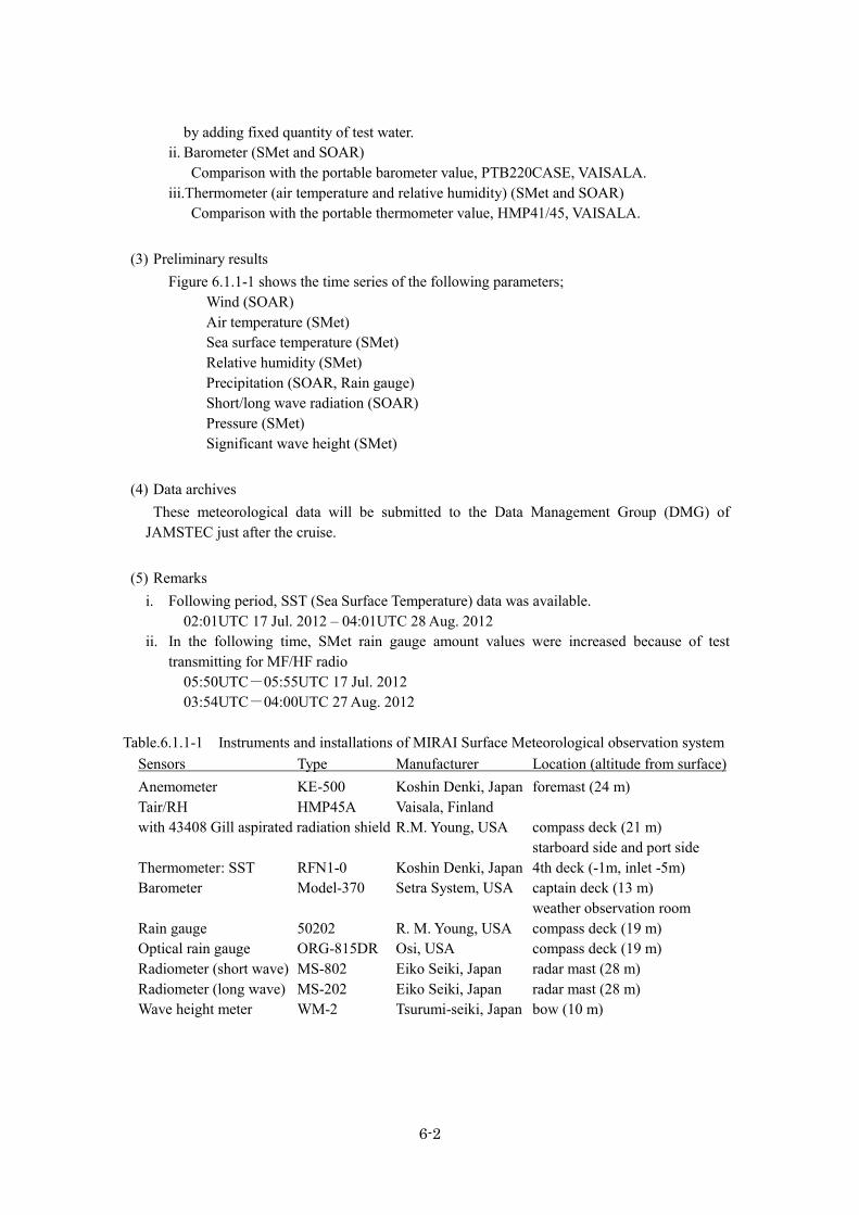
by adding fixed quantity of test water. ii. Barometer (SMet and SOAR)

Comparison with the portable barometer value, PTB220CASE, VAISALA. iii.Thermometer (air temperature and relative humidity) (SMet and SOAR)

Comparison with the portable thermometer value, HMP41/45, VAISALA. (3) Preliminary results

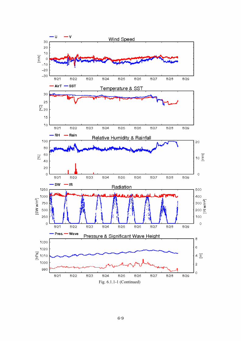
Figure 6.1.1-1 shows the time series of the following parameters; Wind (SOAR) Air temperature (SMet) Sea surface temperature (SMet) Relative humidity (SMet) Precipitation (SOAR, Rain gauge) Short/long wave radiation (SOAR) Pressure (SMet) Significant wave height (SMet)

(4) Data archives

These meteorological data will be submitted to the Data Management Group (DMG) of JAMSTEC just after the cruise.

(5) Remarks

i. Following period, SST (Sea Surface Temperature) data was available. 02:01UTC 17 Jul. 2012 – 04:01UTC 28 Aug. 2012

ii. In the following time, SMet rain gauge amount values were increased because of test transmitting for MF/HF radio

05:50UTC－05:55UTC 17 Jul. 2012 03:54UTC－04:00UTC 27 Aug. 2012

Table.6.1.1-1 Instruments and installations of MIRAI Surface Meteorological observation system

Sensors Type Manufacturer Location (altitude from surface) Anemometer KE-500 Koshin Denki, Japan foremast (24 m) Tair/RH HMP45A Vaisala, Finland with 43408 Gill aspirated radiation shield R.M. Young, USA compass deck (21 m) starboard side and port side Thermometer: SST RFN1-0 Koshin Denki, Japan 4th deck (-1m, inlet -5m) Barometer Model-370 Setra System, USA captain deck (13 m) weather observation room Rain gauge 50202 R. M. Young, USA compass deck (19 m) Optical rain gauge ORG-815DR Osi, USA compass deck (19 m) Radiometer (short wave) MS-802 Eiko Seiki, Japan radar mast (28 m) Radiometer (long wave) MS-202 Eiko Seiki, Japan radar mast (28 m) Wave height meter WM-2 Tsurumi-seiki, Japan bow (10 m)

6-3

Table.6.1.1-2 Parameters of MIRAI Surface Meteorological observation system Parameter Units Remarks 1 Latitude degree 2 Longitude degree 3 Ship’s speed knot MIRAI log, DS-30 Furuno 4 Ship’s heading degree MIRAI gyro, TG-6000, Tokimec 5 Relative wind speed m/s 6sec./10min. averaged 6 Relative wind direction degree 6sec./10min. averaged 7 True wind speed m/s 6sec./10min. averaged 8 True wind direction degree 6sec./10min. averaged 9 Barometric pressure hPa adjusted to sea surface level

6sec. averaged 10 Air temperature (starboard side) degC 6sec. averaged 11 Air temperature (port side) degC 6sec. averaged 12 Dewpoint temperature (starboard side) degC 6sec. averaged 13 Dewpoint temperature (port side) degC 6sec. averaged 14 Relative humidity (starboard side) % 6sec. averaged 15 Relative humidity (port side) % 6sec. averaged 16 Sea surface temperature degC 6sec. averaged 17 Rain rate (optical rain gauge) mm/hr hourly accumulation 18 Rain rate (capacitive rain gauge) mm/hr hourly accumulation 19 Down welling shortwave radiation W/m2 6sec. averaged 20 Down welling infra-red radiation W/m2 6sec. averaged 21 Significant wave height (bow) m hourly 22 Significant wave height (aft) m hourly 23 Significant wave period (bow) second hourly 24 Significant wave period (aft) second hourly

Table.6.1.1-3 Instruments and installation locations of SOAR system

Sensors (Zeno/Met) Type Manufacturer Location (altitude from surface) Anemometer 05106 R.M. Young, USA foremast (25 m) Tair/RH HMP45A Vaisala, Finland with 43408 Gill aspirated radiation shield R.M. Young, USA foremast (23 m) Barometer 61202V R.M. Young, USA with 61002 Gill pressure port R.M. Young, USA foremast (23 m) Rain gauge 50202 R.M. Young, USA foremast (24 m) Optical rain gauge ORG-815DA Osi, USA foremast (24 m) Sensors (PRP) Type Manufacturer Location (altitude from surface) Radiometer (short wave) PSP Epply Labs, USA foremast (25 m) Radiometer (long wave) PIR Epply Labs, USA foremast (25 m) Fast rotating shadowband radiometer Yankee, USA foremast (25 m)

Table.6.1.1-4 Parameters of SOAR system

6-4

Parameter Units Remarks 1 Latitude degree 2 Longitude degree 3 SOG knot 4 COG degree 5 Relative wind speed m/s 6 Relative wind direction degree 7 Barometric pressure hPa 8 Air temperature degC 9 Relative humidity %

10 Rain rate (optical rain gauge) mm/hr 11 Precipitation (capacitive rain gauge) mm reset at 50 mm 12 Down welling shortwave radiation W/m2 13 Down welling infra-red radiation W/m2 14 Defuse irradiance W/m2

6-5

Fig.6.1.1-1 Time series of surface meteorological parameters during the MR12-03 cruise

6-6

Fig. 6.1.1-1 (Continued)

6-7


6-8


6-9


6-10

6.1.2 Ceilometer Yuji Kashino (JAMSTEC) : Principal Investigator Wataru Tokunaga (Global Ocean Development Inc., GODI) Harumi Ota (GODI) Koichi Inagaki (GODI) Ryo Ohyama (MIRAI Crew)

(1) Objectives

The information of cloud base height and the liquid water amount around cloud base is important to understand the process on formation of the cloud. As one of the methods to measure them, the ceilometer observation was carried out.

(2) Parameters 1. Cloud base height [m]. 2. Backscatter profile, sensitivity and range normalized at 30 m resolution. 3. Estimated cloud amount [oktas] and height [m]; Sky Condition Algorithm.

(3) Methods

We measured cloud base height and backscatter profile using ceilometer (CT-25K, VAISALA, Finland) throughout the MR12-03 cruise.

Major parameters for the measurement configuration are as follows;

Laser source: Indium Gallium Arsenide (InGaAs) Diode Transmitting wavelength: 905±5 mm at 25 degC Transmitting average power: 8.9 mW Repetition rate: 5.57 kHz Detector: Silicon avalanche photodiode (APD) Responsibility at 905 nm: 65 A/W Measurement range: 0 ~ 7.5 km Resolution: 50 ft in full range Sampling rate: 60 sec Sky Condition 0, 1, 3, 5, 7, 8 oktas (9: Vertical Visibility) (0: Sky Clear, 1:Few, 3:Scattered, 5-7: Broken, 8: Overcast)

On the archive dataset, cloud base height and backscatter profile are recorded with the resolution of 30 m (100 ft).

(4) Preliminary results

Fig.6.1.2-1 shows the time series of the lowest, second and third cloud base height during the cruise.

(5) Data archives

The raw data obtained during this cruise will be submitted to the Data Management Group

6-11

(DMG) in JAMSTEC.

(7) Remarks 1. Window cleaning;

23:20UTC 16 Jul. 2012, 04:52UTC 23 Jul. 2012, 03:49UTC 25 Jul. 2012, 21:10UTC 28 Jul. 2012, 03:03UTC 31 Jul. 2012, 03:01UTC 02 Aug. 2012 02:30UTC 11 Aug. 2012, 01:37UTC 17 Aug. 2012, 03:59UTC 24 Aug. 2012 2. Following period, data acquisition was suspended because of PC trouble. 00:00UTC 22 Jul. 2012 - 00:22UTC 23 Jul. 2012

6-12

Fig. 6.1.2-1 Lowest, 2nd and 3rd cloud base height during the MR12-03 cruise

6-13


6-14

6.2 CTD/XCTD 6.2.1 CTD (1) Personnel

Yuji Kashino (JAMSTEC): Principal investigator Shungo Oshitani (MWJ): Operation leader Hiroshi Matsunaga (MWJ) Tomohide Noguchi (MWJ) Tamami Ueno (MWJ) Rei Ito (MWJ) Minoru Kamata (MWJ) Shoko Tatamisashi (MWJ) Hatsumi Aoyama (MWJ)

(2) Objective

Investigation of oceanic structure and water sampling. (3) Parameters

Temperature (Primary and Secondary) Conductivity (Primary and Secondary) Pressure Dissolved Oxygen (Primary only)

(4) Instruments and Methods

CTD/Carousel Water Sampling System, which is a 36-position Carousel water sampler (CWS) with Sea-Bird Electronics, Inc. CTD (SBE9plus), was used during this cruise. 12-litter Niskin Bottles were used for sampling seawater. The sensors attached on the CTD were temperature (Primary and Secondary), conductivity (Primary and Secondary), and pressure and dissolved oxygen (Primary). Salinity was calculated by measured values of pressure, conductivity and temperature. The CTD/CWS was deployed from starboard on working deck.

The CTD raw data were acquired on real time using the Seasave-Win32 (ver.7.21h) provided by Sea-Bird Electronics, Inc. and stored on the hard disk of the personal computer. Seawater was sampled during the up cast by sending fire commands from the personal computer. We usually stop for 30 seconds to stabilize then fire.

43 casts of CTD measurements were conducted (Table 6.2.1-1). Data processing procedures and used utilities of SBE Data Processing-Win32 (ver.7.18d) and

SEASOFT were as follows:

(The process in order) DATCNV: Convert the binary raw data to engineering unit data. DATCNV also extracts

bottle information where scans were marked with the bottle confirm bit during acquisition. The duration was set to 3.0 seconds, and the offset was set to 0.0

6-15

seconds.

BOTTLESUM: Create a summary of the bottle data. The data were averaged over 3.0 seconds.

ALIGNCTD: Convert the time-sequence of sensor outputs into the pressure sequence to

ensure that all calculations were made using measurements from the same parcel of water. Dissolved oxygen data are systematically delayed with respect to depth mainly because of the long time constant of the dissolved oxygen sensor and of an additional delay from the transit time of water in the pumped pluming line. This delay was compensated by 6 seconds advancing dissolved oxygen sensor output (dissolved oxygen voltage) relative to the temperature data.

WILDEDIT: Mark extreme outliers in the data files. The first pass of WILDEDIT obtained an

accurate estimate of the true standard deviation of the data. The data were read in blocks of 1000 scans. Data greater than 10 standard deviations were flagged. The second pass computed a standard deviation over the same 1000 scans excluding the flagged values. Values greater than 20 standard deviations were marked bad. This process was applied to pressure, depth, temperature, conductivity dissolved oxygen voltage and decent rate.

CELLTM: Remove conductivity cell thermal mass effects from the measured conductivity.

Typical values used were thermal anomaly amplitude alpha = 0.03 and the time constant 1/beta = 7.0.

FILTER: Perform a low pass filter on pressure with a time constant of 0.15 second. In order to

produce zero phase lag (no time shift) the filter runs forward first then backward

SECTIONU (original module of SECTION): Select a time span of data based on scan number in order to reduce a file size. The minimum number was set to be the starting time when the CTD package was beneath the sea-surface after activation of the pump. The maximum number of was set to be the end time when the package came up from the surface.

LOOPEDIT: Mark scans where the CTD was moving less than the minimum velocity of 0.0 m/s

(traveling backwards due to ship roll). DERIVE: Compute dissolved oxygen (SBE43). BINAVG: Average the data into 1-dbar pressure bins.

6-16

DERIVE: Compute salinity, potential temperature, and sigma-theta. SPLIT: Separate the data from an input .cnv file into down cast and up cast files. Configuration file: MR1203A.con Specifications of the sensors are listed below.

CTD: SBE911plus CTD system Under water unit:

SBE9plus S/N 09P38273-0786 (Sea-Bird Electronics, Inc.)

Pressure sensor: Digiquartz pressure sensor (S/N 94766) Calibrated Date: 30 Jun. 2012

Temperature sensors: Primary: SBE03-04/F (S/N 031464, Sea-Bird Electronics, Inc.)

Calibrated Date: 15 Dec. 2011 Secondary: SBE03Plus (S/N 03P2730, Sea-Bird Electronics, Inc.)

Calibrated Date: 18 Apr. 2012 Conductivity sensors:

Primary: SBE04-04/0 (S/N 041203, Sea-Bird Electronics, Inc.) Calibrated Date: 18 Apr. 2012

Secondary: SBE04-04/0 (S/N 041172, Sea-Bird Electronics, Inc.) Calibrated Date: 18 Apr. 2012

Dissolved Oxygen sensors: Primary: SBE43 (S/N 43330, Sea-Bird Electronics, Inc.)

Calibrated Date: 01 May. 2012 Carousel water sampler:

SBE32 (S/N 3221746-0278, Sea-Bird Electronics, Inc.)

Deck unit: SBE11plus (S/N 11P7030-0272, Sea-Bird Electronics, Inc.) (5) Preliminary Results

During this cruise, 43casts of CTD observation were carried out. Date, time and locations of the CTD casts are listed in Table 6.2.1-1.

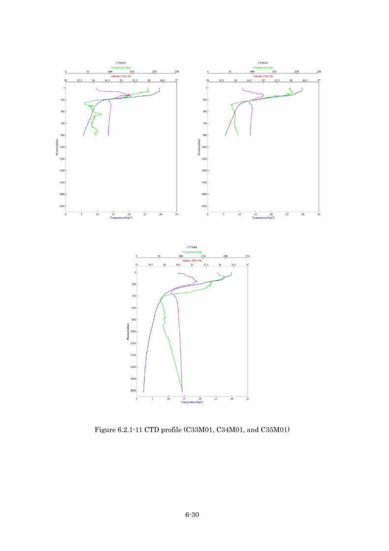
Vertical profile (down cast) of primary temperature, salinity and dissolved oxygen with pressure are shown in Figure 6.2.1-1 - 6.2.1-11

In the down cast of Stn.C21 (filename: C21M01) and Stn.C31 (filename: C31M01), spike was observed in the dissolved oxygen sensor. (6) Data archive

All raw and processed data files were copied onto HD provided by Data Management Office (DMO); JAMSTEC will be opened to public via “R/V MIRAI Data Web Page” in the JAMSTEC home page.

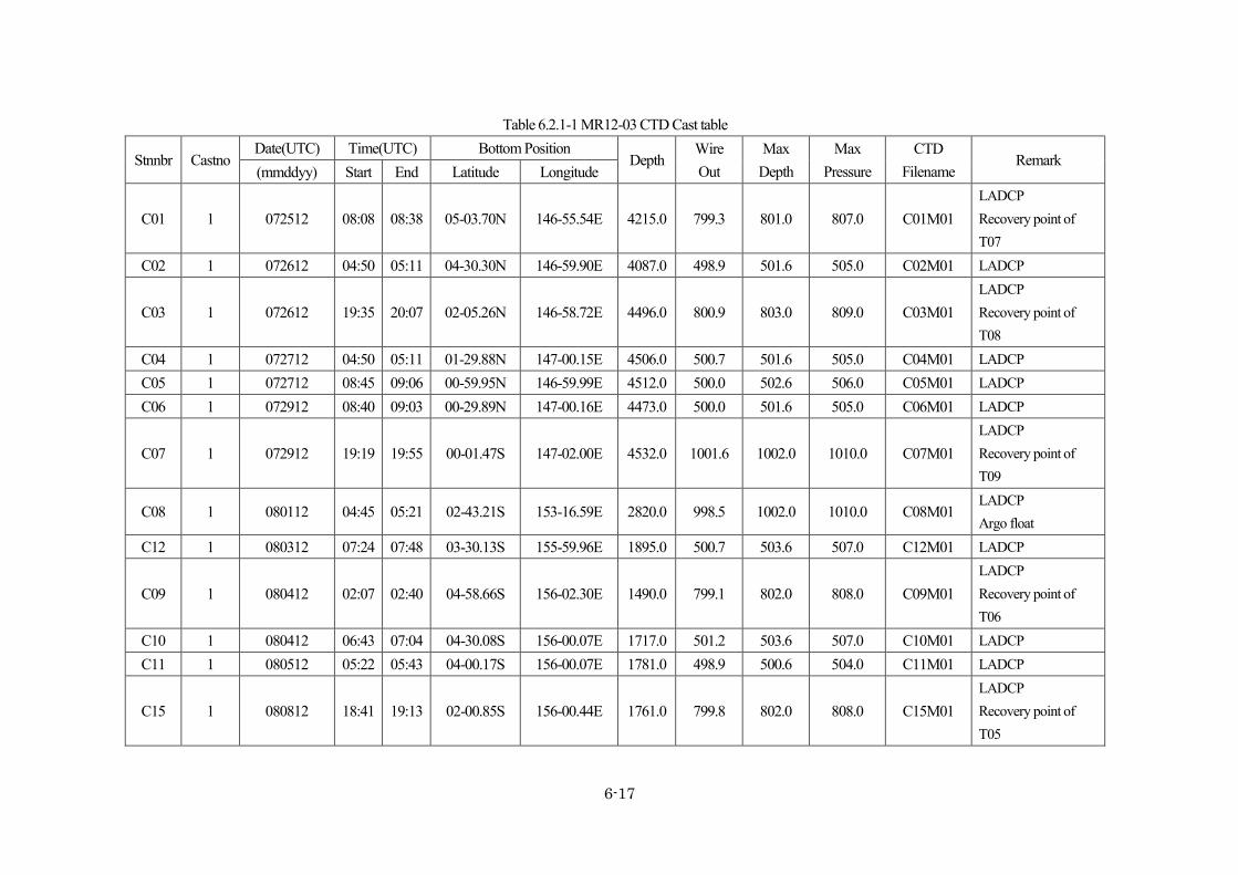
6-17

Table 6.2.1-1 MR12-03 CTD Cast table

Stnnbr Castno Date(UTC) Time(UTC) Bottom Position

Depth Wire Out

Max Depth

Max Pressure

CTD Filename

Remark (mmddyy) Start End Latitude Longitude

C01 1 072512 08:08 08:38 05-03.70N 146-55.54E 4215.0 799.3 801.0 807.0 C01M01 LADCP Recovery point of T07

C02 1 072612 04:50 05:11 04-30.30N 146-59.90E 4087.0 498.9 501.6 505.0 C02M01 LADCP


C04 1 072712 04:50 05:11 01-29.88N 147-00.15E 4506.0 500.7 501.6 505.0 C04M01 LADCP C05 1 072712 08:45 09:06 00-59.95N 146-59.99E 4512.0 500.0 502.6 506.0 C05M01 LADCP

C06 1 072912 08:40 09:03 00-29.89N 147-00.16E 4473.0 500.0 501.6 505.0 C06M01 LADCP

C07 1 072912 19:19 19:55 00-01.47S 147-02.00E 4532.0 1001.6 1002.0 1010.0 C07M01 LADCP Recovery point of T09

C08 1 080112 04:45 05:21 02-43.21S 153-16.59E 2820.0 998.5 1002.0 1010.0 C08M01 LADCP Argo float

C12 1 080312 07:24 07:48 03-30.13S 155-59.96E 1895.0 500.7 503.6 507.0 C12M01 LADCP


C10 1 080412 06:43 07:04 04-30.08S 156-00.07E 1717.0 501.2 503.6 507.0 C10M01 LADCP C11 1 080512 05:22 05:43 04-00.17S 156-00.07E 1781.0 498.9 500.6 504.0 C11M01 LADCP


6-18



C18 1 081212 06:29 06:51 00-30.15S 156-00.09E 1953.0 499.2 501.6 505.0 C18M01 LADCP

C19 1 081212 19:03 19:27 00-00.00S 155-59.97E 1953.0 499.6 500.6 504.0 C19M01 LADCP C19 2 081212 22:03 22:25 00-00.11N 156-00.59E 1954.0 499.6 501.6 505.0 C19M02 LADCP


C19 5 081312 07:01 07:23 00-00.00N 155-59.96E 1953.0 500.0 500.6 504.0 C19M05 LADCP C19 6 081312 10:01 10:23 00-00.15S 155-59.80E 1950.0 500.7 502.6 506.0 C19M06 LADCP

C19 7 081312 13:00 13:21 00-00.12N 155-59.38E 1952.0 502.3 501.6 505.0 C19M07 LADCP



C22 1 081412 06:50 07:13 00-45.14N 156-00.14E 2152.0 502.5 502.6 506.0 C22M01 LADCP




C28 1 081512 05:16 05:38 02-30.05N 156-00.10E 2676.0 498.9 501.6 505.0 C28M01 LADCP

C29 1 081612 06:29 06:52 02-59.94N 156-00.06E 2875.0 500.5 502.7 506.0 C29M01 LADCP

6-19

C30 1 081712 07:49 08:11 03-30.12N 156-00.05E 3251.0 499.8 501.6 505.0 C30M01 LADCP




C35 1 082112 22:46 23:49 12-00.04N 154-18.05E 5923.0 2002.0 2001.8 2023.0 C35M01

6-20

Figure 6.2.1-1 CTD profile (C01M01, C02M01, C03M01 and C04M01)

6-21


6-22


6-23


6-24


6-25


6-26


6-27


6-28


6-29


6-30

Figure 6.2.1-11 CTD profile (C33M01, C34M01, and C35M01)

6-31

6.2.2 XCTD (1) Personnel

Yuji Kashino (JAMSTEC): Principal Investigator Takuya Hasegawa (JAMSTEC) Wataru Tokunaga (Global Ocean Development Inc.: GODI) Harumi Ota (GODI) Koichi Inagaki (GODI) Ryo Ohyama (MIRAI Crew)

(2) Objectives

Investigation of oceanic structure. (3) Parameters

According to the manufacturer’s nominal specifications, the range and accuracy of parameters measured by the XCTD (eXpendable Conductivity, Temperature & Depth profiler) are as follows;

Parameter Range Accuracy Conductivity 0 ~ 60 [mS/cm] +/- 0.03 [mS/cm] Temperature -2 ~ 35 [deg-C] +/- 0.02 [deg-C] Depth 0 ~ 1000 [m] 5 [m] or 2 [%] (either of them is major)

(4) Methods

We observed the vertical profiles of the sea water temperature and salinity measured by XCTD-1 manufactured by Tsurumi-Seiki Co.. The signal was converted by MK-150N, Tsurumi-Seiki Co. and was recorded by AL12 software (Ver.1.1.4) provided by Tsurumi-Seiki Co.. We launched 36 probes (X01-X36) by an automatic launcher. The summary of XCTD observations and launching log were shown in Table 6.2.2. SST (Sea Surface Temperature) and SSS (Sea Surface Salinity) in the table were got from TSG (ThermoSalinoGraph) at launching.


Position map of XCTD observations was shown in Fig. 6.2.2-1. Vertical section of temperature and salinity were shown in Fig.6.2.2-2 and Fig.6.2.2-3.

(6) Data archive

These data obtained in this cruise will be submitted to the Data Management Group (DMG) of JAMSTEC, and will be opened to the public via “R/V MIRAI Data Web Page” in JAMSTEC home page.

6-32

Table 6.2.2 Summary of XCTD observation and launching log

Station No.

Date (UTC)

Time (UTC) Latitude Longitude Depth

[m] SST

[deg-C] SSS

[PSU] Probe S/N

X01 2012/07/25 06:51 04-58.00N 147-00.70E 4290 29.578 34.178 12057601

X02 2012/07/26 08:41 03-59.96N 147-00.01E 4668 29.473 34.148 12057604

X03 2012/07/26 11:21 03-29.98N 146-59.98E 4281 29.503 34.148 12057605

X04 2012/07/26 14:03 03-00.00N 146-59.97E 4428 29.199 33.866 12057603

X05 2012/07/26 16:40 02-30.00N 146-59.93E 4423 29.338 34.040 12057602

X06 2012/07/28 03:35 02-04.35N 146-56.82E 4490 29.384 34.151 12057606

X07 2012/07/29 01:18 00-03.21N 147-02.00E 4479 29.091 33.831 12057607

X08 2012/07/31 22:11 02-14.02S 153-38.01E 3830 29.021 34.677 12057609

X09 2012/08/01 00:05 02-30.02S 153-25.99E 4507 29.153 34.725 12057608

X10 2012/08/01 06:03 02-48.31S 153-13.21E 3473 29.451 34.615 12057612

X11 2012/08/01 07:48 03-03.00S 153-01.03E 2337 29.236 34.825 12057611

X12 2012/08/01 09:43 03-20.00S 152-49.02E 2266 29.198 34.823 12057610

X13 2012/08/01 11:37 03-35.97S 152-37.00E 1065 29.222 34.820 12057613

X14 2012/08/02 05:03 03-50.24S 152-56.01E 2412 29.502 34.855 12057614

X15 2012/08/02 07：08 04-05.28S 153-15.02E 2638 29.271 34.811 12057618

X16 2012/0802 09：17 04-19.92S 153-34.00E 3532 28.575 34.591 12057617

X17 2012/08/02 11：25 04-34.31S 153-53.01E 3817 29.002 34.753 12057621

X18 2012/08/02 13：18 04-47.44S 154-09.00E 2931 29.043 34.777 12057622

X19 2012/08/02 15：19 04-59.88S 154-25.00E 1052 29.299 34.696 12057615

X20 2012/08/02 17：13 04-57.97S 154-44.01E 2343 29.160 34.695 12057616

X21 2012/08/02 19：00 05-00.00S 155-03.00E 3298 29.511 34.588 12057619

X22 2012/08/02 20：45 05-00.00S 155-22.00E 3013 29.410 34.726 12057620

X23 2012/08/02 22：27 05-00.00S 155-41.00E 2053 29.195 34.673 12057623

X24 2012/08/04 10：37 05-01.93S 156-02.49E 1509 29.429 34.697 12057624

X25 2012/08/10 01：26 02-01.02S 155-57.96E 1758 29.223 34.646 12036649

X26 2012/08/10 23：21 00-00.22N 156-03.29E 1950 19.129 33.825 12036650

X27 2012/08/16 01：28 02-02.23N 156-00.74E 2579 29.147 34.003 12057627

X28 2012/08/19 01：23 05-01.06N 155-58.54E 3607 29.694 34.152 12057628

X29 2012/08/19 04：09 05-30.00N 156-00.00E 3737 29.869 34.051 12057630

X30 2012/08/19 06：55 06-00.15N 156-00.00E 4150 29.979 34.092 12057629

X31 2012/08/19 09：34 06-29.97N 156-00.03E 4413 29.877 34.087 12057631

X32 2012/08/19 12：08 07-00.20N 156-00.00E 4435 29.739 34.085 12057632

X33 2012/08/19 14：52 07-30.00N 155-59.99E 4396 29.802 34.088 12057635

X34 2012/08/19 18：19 07-58.60N 156-00.75E 4838 29.722 34.241 12057634

X35 2012/08/19 18：51 07-58.61N 156-00.75E 4839 29.716 34.241 12057633

X36 2012/08/21 01：39 07-57.89N 156-02.62E 4830 29.951 34.199 12057636

6-33

Fig. 6.2.2-1 Position map of XCTD observations.

6-34

Fig. 6.2.2-2 Vertical section of temperature (upper) and salinity (lower) along 147E(X01 to X07)

6-35

Fig. 6.2.2-3 Vertical section of temperature (upper) and salinity (lower) along 156E(X24 to X36)

6-36

6.3 Water sampling 6.3.1 Salinity (1) Personnel Yuji Kashino (JAMSTEC) : Principal Investigator Tamami Ueno (MWJ) : Technical Staff (Operation Leader) Hiroki Ushiromura （MWJ） : Technical Staff (2) Objective To measure bottle salinity obtained by CTD casts and The Continuous Sea Surface Water Monitoring System (TSG). (3) Method a. Salinity Sample Collection

Seawater samples were collected with 12 liter Niskin-X bottles and TSG. The salinity sample bottle of the 250ml brown glass with screw cap was used collecting the sample seawater. Each bottle was rinsed three times with the sample seawater, and was filled with sample seawater to the bottle shoulder. In this cruise, each bottle sealed with a plastic insert cap and a screw cap because we took into consideration the possibility of storage for about two weeks. These caps were rinsed three times with the sample seawater before its use. Each bottle was stored for more than 12 hours in the laboratory before the salinity measurement. The kind and number of samples taken are shown as follows；

Table 6.3.1-1 Kind and number of samples Kind of Samples Number of Samples Samples for CTD 86 Samples for TSG 41

Total 127 b. Instruments and Method

The salinity measurement was carried out on R/V MIRAI during the cruise of MR12-03 using the salinometer (Model 8400B “AUTOSAL”； Guildline Instruments Ltd.: S/N 62556) with an additional peristaltic-type intake pump (Ocean Scientific International, Ltd.). A pair of precision digital thermometers (Model 9540； Guildline Instruments Ltd.) were used. One thermometer monitored the ambient temperature and the other monitored the bath temperature of the salinometer. The specifications of the AUTOSAL salinometer and thermometer are shown as follows；

Salinometer (Model 8400B “AUTOSAL”； Guildline Instruments Ltd.) Measurement Range ： 0.005 to 42 (PSU) Accuracy ： Better than ±0.002 (PSU) over 24 hours

without re-standardization Maximum Resolution ： Better than ±0.0002 (PSU) at 35 (PSU)

6-37

Thermometer (Model 9540； Guildline Instruments Ltd.) Measurement Range ： -40 to +180 deg C

Resolution ： 0.001 Limits of error ±deg C ： 0.01 (24 hours @ 23 deg C ±1 deg C) Repeatability ： ±2 least significant digits

The measurement system was almost the same as Aoyama et al. (2002). The salinometer was operated in the air-conditioned ship's laboratory at a bath temperature of 24 deg C. The ambient temperature varied from approximately 22 deg C to 25 deg C, while the bath temperature was very stable and varied within +/- 0.002 deg C on rare occasion. The measurement for each sample was done with a double conductivity ratio and defined as the median of 31 readings of the salinometer. Data collection was started 10 seconds after filling the cell with the sample and it took about 15 seconds to collect 31 readings by a personal computer. Data were taken for the sixth and seventh filling of the cell. In the case of the difference between the double conductivity ratio of these two fillings being smaller than 0.00002, the average value of the double conductivity ratio was used to calculate the bottle salinity with the algorithm for the practical salinity scale, 1978 (UNESCO, 1981). If the difference was greater than or equal to 0.00003, an eighth filling of the cell was done. In the case of the difference between the double conductivity ratio of these two fillings being smaller than 0.00002, the average value of the double conductivity ratio was used to calculate the bottle salinity. In the case of the double conductivity ratio of eighth filling did not satisfy the criteria, we measured a ninth filling of the cell and calculated the bottle salinity. The measurement was conducted in about 5 hours per day and the cell was cleaned with soap after the measurement of the day.

(4) Preliminary Results a. Standard Seawater

Standardization control of the salinometer was set to 696 at 26th July. But soon the value of SSW was off the point. So standardization control of the salinometer was set again to 693 at 28th July. After the day, the value of STANDBY was 24+5200~5201 and that of ZERO was 0.0-0001~0000.

In this cruise, the conductivity ratio of IAPSO Standard Seawater batch P154 was 0.99990 (the double conductivity ratio was 1.99980) and was used as the standard for salinity.

The specifications of SSW used in this cruise are shown as follows； Batch ： P154 Conductivity Ratio ： 0.99990 Salinity ： 34.996 Use By ： 20th October 2014

6-38

Fig.6.3.1 shows the double conductivity ratio of the Standard Seawater. Figure (a) shows before correction. The average of the double conductivity ratio was 1.99986 and the standard deviation was 0.00003, which is equivalent to 0.0006 in salinity. Figure (b) shows after correction. The average of the double conductivity ratio was 1.99980 and the standard deviation was 0.00001, which is equivalent to 0.0002 in salinity.

Fig. 6.3.1(a) Time series of double conductivity ratio for the Standard Seawater (before correction)

Fig.6.3.1(b) Time series of double conductivity ratio for the Standard Seawater (after correction)

6-39

b. Sub-Standard Seawater Sub-standard seawater was made from deep-sea water filtered by a pore size of 0.45 micrometer and stored in a 20 liter container made of polyethylene and stirred for at least 24 hours before measuring. It was measured about every 6 samples in order to check for the possible sudden drifts of the salinometer.

c. Replicate Samples

We estimated the precision of this method using 43 pairs of replicate samples taken from the same Niskin bottle. Fig.6.3.2 shows the histogram of the absolute difference between each pair of the replicate samples. The average and the standard deviation of absolute difference among 43 pairs of replicate samples were 0.0003 and 0.0003 in salinity, respectively.

Fig.6.3.2 The histogram of the double conductivity ratio for the absolute difference of replicate samples

6-40

5) Data archive These raw datasets will be submitted to JAMSTEC Data Management Office (DMO). (6) Reference ・Aoyama, M. T. Joyce, T. Kawano and Y. Takatsuki : Standard seawater comparison up to P129.

Deep-Sea Research, I, Vol. 49, 1103～1114, 2002 ・UNESCO : Tenth report of the Joint Panel on Oceanographic Tables and Standards.

UNESCO Tech. Papers in Mar. Sci., 36, 25 pp., 1981

6-41

6.4 Continuous monitoring of surface seawater 6.4.1 Temperature, salinity, dissolved oxygen

1. Personnel

Yuji Kashino (JAMSTEC): Principal Investigator Shoko Tatamisashi (MWJ)

2. Objective

Our purpose is to obtain salinity, temperature and dissolved oxygen data continuously in near-sea

surface water.

3. Instruments and Methods

The Continuous Sea Surface Water Monitoring System (Marine Works Japan Co. Ltd.) has four

sensors and automatically measures salinity, temperature and dissolved oxygen in near-sea surface

water every one minute. This system is located in the “sea surface monitoring laboratory” and

connected to shipboard LAN-system. Measured data, time, and location of the ship were stored in a

data management PC. The near-surface water was continuously pumped up to the laboratory from

about 5 m water depth and flowed into the system through a vinyl-chloride pipe. The flow rate of

the surface seawater was adjusted to be 3 dm3 min-1. Specifications of the each sensor in this

system are listed below.

a. Instruments

Software

Seamoni-kun Ver.1.20

Sensors

Specifications of the each sensor in this system are listed below.

Temperature and Conductivity sensor

Model: SBE-45, SEA-BIRD ELECTRONICS, INC.

Serial number: 4552788-0264

Measurement range: Temperature -5 to +35 oC

Conductivity 0 to 7 S m-1

Initial accuracy: Temperature 0.002 oC

Conductivity 0.0003 S m-1

6-42

Typical stability (per month): Temperature 0.0002 oC


Resolution: Temperatures 0.0001 oC


Bottom of ship thermometer

Model: SBE 38, SEA-BIRD ELECTRONICS, INC.

Serial number: 3852788-0457

Measurement range: -5 to +35 oC

Initial accuracy: ±0.001 oC

Typical stability (per 6 month): 0.001 oC

Resolution: 0.00025 oC

Dissolved oxygen sensor

Model: OPTODE 3835, AANDERAA Instruments.

Serial number: 1233

Measuring range: 0 - 500 µmol dm-3

Resolution: <1 µmol dm-3

Accuracy: <8 µmol dm-3 or 5% whichever is greater

Settling time: <25 s

4. Measurements

Periods of measurement, maintenance, and problems during MR12-03 are listed in Table 6.4.1-1.

Table 6.4.1-1 Events list of the surface seawater monitoring during MR12-03

System Date

[UTC]

System Time

[UTC]

Events Remarks

2012/07/17 2:35 Start up a system.

Check the logging data.

2012/07/17 3:00 All of the measurements started and

data was available.

2012/08/28 04:00 All the measurements stopped.

6-43

5. Preliminary Result

We took the surface water samples to compare sensor data with bottle data of salinity. The

results are shown in Fig.6.4.1-1. All the salinity samples were analyzed by the Guideline 8400B

“AUTOSAL”. Preliminary data of temperature, salinity, and dissolved oxygen at sea surface are

shown in Fig.6.4.1-2.

6. Data archive

These data obtained in this cruise will be submitted to the Data Management Office (DMO) of

JAMSTEC, and will be opened to the public via “R/V Mirai Data Web Page” in JAMSTEC home

page.

Fig.6.4.1-1 Correlation of salinity between sensor data and bottle data.

6-44

(a) Temperature

(b) Salinity

(c) Dissolved oxygen

Fig.6.4.1-2 Spatial and temporal distribution of (a) temperature (b) salinity (c) dissolved oxygen in

MR12-03 cruise.

6-45

6.5 Underway pCO2

Shuji KAWAKAMI (JAXA): Principal Investigator Yoshiyuki NAKANO (JAMSTEC MIO) Hatsumi AOYAMA(MWJ): Operation Leader Minoru KAMATA(MWJ) (1) Objectives

Concentrations of CO2 in the atmosphere are increasing at a rate of 1.5 ppmv yr–1 owing to human activities such as burning of fossil fuels, deforestation, and cement production. Oceanic CO2 concentration is also considered to be increased with the atmospheric CO2 increase, however, its variation is widely different by time and locations. Underway pCO2 observation is indispensable to know the pCO2 distribution, and it leads to elucidate the mechanism of oceanic pCO2 variation. We here report the underway pCO2 measurements performed during MR12-03 cruise. (2) Methods, Apparatus and Performance Oceanic and atmospheric CO2 concentrations were measured during the cruise using an automated system equipped with a non-dispersive infrared gas analyzer (NDIR; LI-7000, Li-Cor). Measurements were done every about one and a half hour, and 4 standard gases, atmospheric air, and the CO2 equilibrated air with sea surface water were analyzed subsequently in this hour. The concentrations of the CO2 standard gases were 300.08, 349.96, 399.98 and 450.23 ppmv. Atmospheric air taken from the bow of the ship (approx.30 m above the sea level) was introduced into the NDIR by passing through a electrical cooling unit, a mass flow controller which controls the air flow rate of 0.5 L min-1, a membrane dryer (MD-110-72P, perma pure llc.) and chemical desiccant (Mg(ClO4)2). The CO2 equilibrated air was the air with its CO2 concentration was equivalent to the sea surface water. Seawater was taken from an intake placed at the approximately 4.5 m below the sea surface and introduced into the equilibrator at the flow rate of 4 - 5 L min-1 by a pump. The equilibrated air was circulated in a closed loop by a pump at flow rate of 0.6 - 0.8 L min-1 through two cooling units, a membrane dryer, the chemical desiccant, and the NDIR. (3) Preliminary results

Cruise track during pCO2 observation is shown in Figure 6.5-1. Temporal variations of both oceanic and atmospheric CO2 concentration (xCO2) are shown in Fig. 6.5-2. (4) Data Archive Data obtained in this cruise will be submitted to the Data Management Office (DMO) of JAMSTEC, and will be opened to the public via “R/V Mirai Data Web Page” in JAMSTEC home page. (5) Reference Dickson, A. G., Sabine, C. L. & Christian, J. R. (2007), Guide to best practices for ocean CO2 measurements; PICES Special Publication 3, 199pp.

6-46

Figure 6.5-1 Observation map

Figure 6.5-1 Temporal variations of oceanic and atmospheric CO2 concentration (xCO2). Blue dots represent oceanic xCO2 variation and green atmospheric xCO2. SST variation (red) is also shown.

6-47

6.6 Shipboard ADCP (1) Personnel

Yuji Kashino (JAMSTEC): Principal Investigator Wataru Tokunaga (Global Ocean Development Inc., GODI) Harumi Ota (GODI) Koichi Inagaki (GODI) Ryo Ohyama (MIRAI Crew)

(2) Objective

To obtain continuous measurement of the current profile along the ship’s track. (3) Methods

Upper ocean current measurements were made in MR12-03 cruise, using the hull-mounted Acoustic Doppler Current Profiler (ADCP) system. For most of its operation the instrument was configured for water-tracking mode. Bottom-tracking mode, interleaved bottom-ping with water-ping, was made to get the calibration data for evaluating transducer misalignment angle. The system consists of following components;

1) R/V MIRAI has installed the Ocean Surveyor for vessel-mount (acoustic frequency

76.8 kHz; Teledyne RD Instruments). It has a phased-array transducer with single ceramic assembly and creates 4 acoustic beams electronically. We mounted the transducer head rotated to a ship-relative angle of 45 degrees azimuth from the keel

2) For heading source, we use ship’s gyro compass (Tokimec, Japan), continuously providing heading to the ADCP system directory. Additionally, we have Inertial Navigation System (INS) which provide high-precision heading, attitude information, pitch and roll, are stored in “.N2R” data files with a time stamp.

3) DGPS system (Trimble SPS751 & StarFixXP) providing position fixes. 4) We used VmDas version 1.4.6 (TRD Instruments) for data acquisition. 5) To synchronize time stamp of ping with GPS time, the clock of the logging computer is

adjusted to GPS time every 1 minute 6) We have placed ethylene glycol into the fresh water to prevent freezing in the sea chest. 7) The sound speed at the transducer does affect the vertical bin mapping and vertical

velocity measurement, is calculated from temperature, salinity (constant value; 35.0 psu) and depth (6.5 m; transducer depth) by equation in Medwin (1975).

Data was configured for 16 m intervals starting 16 m below the surface. Every ping was

recorded as raw ensemble data (.ENR). Also, 60 seconds and 300 seconds averaged data were recorded as short term average (.STA) and long term average (.LTA) data, respectively. Major parameters for the measurement (Direct Command) are shown in Table 6.6-1.

6-48


Fig.6.6-1 shows the surface current vector along the ship’s track. (5) Data archive

These data obtained in this cruise will be submitted to the Data Management Group (DMG) of JAMSTEC, and will be opened to the public via JAMSTEC home page.

Table 6.6-1 Major parameters

Bottom-Track Commands BP = 001 Pings per Ensemble (almost less than 1300m depth) 23:32UTC 16 July to 18:06UTC 17 July, 2012 18:56UTC 27 August to 00:11UTC 29 August, 2012

Environmental Sensor Commands EA = +04500 Heading Alignment (1/100 deg) EB = +00000 Heading Bias (1/100 deg) ED = 00065 Transducer Depth (0 - 65535 dm) EF = +001 Pitch/Roll Divisor/Multiplier (pos/neg) [1/99 - 99] EH = 00000 Heading (1/100 deg) ES = 35 Salinity (0-40 pp thousand) EX = 00000 Coord Transform (Xform:Type; Tilts; 3Bm; Map) EZ = 10200010 Sensor Source (C; D; H; P; R; S; T; U) C (1): Sound velocity calculates using ED, ES, ET (temp.) D (0): Manual ED H (2): External synchro P (0), R (0): Manual EP, ER (0 degree) S (0): Manual ES T (1): Internal transducer sensor U (0): Manual EU

Timing Commands TE = 00:00:02.00 Time per Ensemble (hrs:min:sec.sec/100) TP = 00:02.00 Time per Ping (min:sec.sec/100)

Water-Track Commands WA = 255 False Target Threshold (Max) (0-255 count) WB = 1 Mode 1 Bandwidth Control (0=Wid, 1=Med, 2=Nar) WC = 120 Low Correlation Threshold (0-255) WD = 111 100 000 Data Out (V; C; A; PG; St; Vsum; Vsum^2;#G;P0) WE = 1000 Error Velocity Threshold (0-5000 mm/s)

6-49

WF = 0800 Blank After Transmit (cm) WG = 001 Percent Good Minimum (0-100%) WI = 0 Clip Data Past Bottom (0 = OFF, 1 = ON) WJ = 1 Rcvr Gain Select (0 = Low, 1 = High) WM = 1 Profiling Mode (1-8) WN = 40 Number of depth cells (1-128) WP = 00001 Pings per Ensemble (0-16384) WS = 1600 Depth Cell Size (cm) WT = 000 Transmit Length (cm) [0 = Bin Length] WV = 0390 Mode 1 Ambiguity Velocity (cm/s radial)

6-50

Fig 6.6-1. Surface current vector along the ship’s track. (TRITON area)

6-51

6.7 Underway geophysics Personnel Takeshi Hanyu (JAMSTEC) : Principal Investigator Takeshi Matsumoto (University of the Ryukyus) : Principal Investigator (Not on-board) Masao Nakanishi (Chiba University) : Principal Investigator (Not on-board) Wataru Tokunaga (Global Ocean Development Inc., GODI) Harumi Ota (GODI) Koichi Inagaki (GODI) Ryo Ohyama (MIRAI Crew)

6.7.1. Sea surface gravity (1) Introduction

The local gravity is an important parameter in geophysics and geodesy. We collected gravity data at the sea surface.

(2) Parameters

Relative Gravity [CU: Counter Unit] [mGal] = (coef1: 0.9946) * [CU]

(3) Data Acquisition

We measured relative gravity using LaCoste and Romberg air-sea gravity meter S-116 (Micro-g LaCoste, LLC) during the MR12-03 cruise from 17th July 2012 to 29th August 2012.

To convert the relative gravity to absolute one, we measured gravity, using portable gravity meter (Scintrex gravity meter CG-5), at Sekinehama as the reference point.

(4) Preliminary Results

Absolute gravity shown in Tabel 6.7.1-1 (5) Data Archives

Surface gravity data obtained during this cruise will be submitted to the Data Management Group (DMG) in JAMSTEC, and will be archived there.

Table 6.7.1-1

No Date UTC Port Absolute Gravity [mGal]

Sea Level [cm]

Draft [cm]

Gravity at Sensor *1 [mGal]

L&R*2 Gravity [mGal]

#1 July/16 21:50 Sekinehama 980,371.93 316 669 980,372.21 12,614.68 #2 Aug/12 03:33 Sekinehama 980,371.94 243 633 980,372.91 12,610.65

6-52

*1: Gravity at Sensor = Absolute Gravity + Sea Level*0.3086/100 + (Draft-530)/100*0.2222 *2: LaCoste and Romberg air-sea gravity meter S-116

6-53

6.7.2 Sea surface magnetic field 1) Three-component magnetometer (1) Introduction

Measurement of magnetic force on the sea is required for the geophysical investigations of marine magnetic anomaly caused by magnetization in upper crustal structure. We measured geomagnetic field using a three-component magnetometer during the MR12-03 cruise from 17th July 2012 to 29th August 2012.

(2) Principle of ship-board geomagnetic vector measurement

The relation between a magnetic-field vector observed on-board, Hob, (in the ship's fixed coordinate system) and the geomagnetic field vector, F, (in the Earth's fixed coordinate system) is expressed as:

Hob = A R P Y F + Hp (a)

where R, P and Y are the matrices of rotation due to roll, pitch and heading of a ship, respectively. A is a 3 x 3 matrix which represents magnetic susceptibility of the ship, and Hp is a magnetic field vector produced by a permanent magnetic moment of the ship's body. Rearrangement of Eq. (a) makes

R Hob + Hbp = R P Y F (b)

where R = A-1, and Hbp = -R Hp. The magnetic field, F, can be obtained by measuring R, P, Y and Hob, if R and Hbp are known. Twelve constants in R and Hbp can be determined by measuring variation of Hob with R, P and Y at a place where the geomagnetic field, F, is known.

(3) Instruments on R/V MIRAI

A shipboard three-component magnetometer system (Tierra Tecnica SFG1214) is equipped on-board R/V MIRAI. Three-axes flux-gate sensors with ring-cored coils are fixed on the fore mast. Outputs from the sensors are digitized by a 20-bit A/D converter (1 nT/LSB), and sampled at 8 times per second. Ship's heading, pitch, and roll are measured by the Inertial Navigation System (INS) for controlling attitude of a Doppler radar. Ship's position (GPS) and speed data are taken from LAN every second.

(4) Data Archives

These data obtained in this cruise will be submitted to the Data Management Group (DMG) of JAMSTEC.

(5) Remarks

1) For calibration of the ship’s magnetic effect, we made a “figure-eight” turn (a pair of clockwise and anti-clockwise rotation). This calibration was carried out as below.

6-54

27th Jul. 2012, 19:07 – 19:30UTC around at 02-05N, 146-57E 03rd Aug. 2012, 18:28 – 18:53UTC around at 05-02S, 156-01E 07th Aug. 2012, 05:06 – 05:52UTC around at 04-16S, 157-26E 11th Aug. 2012, 06:58 – 07:24UTC around at 00-03S, 155-59E 20th Aug. 2012, 02:40 – 03:17UTC around at 07-57S, 156-00E

2) Cesium magnetometer (1) Introduction

Measurement of total magnetic force on the sea is required for the geophysical investigations of marine magnetic anomaly caused by magnetization in upper crustal structure.

(2) Data Period and Sensor Rotation

30 Jul. 2012, 01:32 – 30 Jul. 2012, 03:02UTC Rotation = 0 degrees 30 Jul. 2012, 03:44 – 31 Jul. 2012, 18:34UTC Rotation = 45 degrees 06 Aug. 2012, 04:43 – 06 Aug. 2012, 19:29UTC Rotation = 0 degrees 07 Aug. 2012, 04:48 – 07 Aug. 2012, 19:29UTC Rotation = 0 degrees

(3) Specification

We measured total geomagnetic field using a cesium marine magnetometer (Geometrics Inc., G-882) and recorded by G-882 data logger (Clovertech Co., Ver.1.0.0). The G-882 magnetometer uses an optically pumped Cesium-vapor atomic resonance system. The sensor fish towed 500 m behind the vessel to minimize the effects of the ship's magnetic field. Table 6.7.2-1 shows system configuration of MIRAI cesium magnetometer system.

Table 6.7.2-1 System configuration of MIRAI cesium magnetometer.

Dynamic operating range: 20,000 to 100,000 nT Absolute accuracy: <±2 nT throughout range Setting: Cycle rate; 0.1 sec Sensitivity; 0.001265 nT at a 0.1 second cycle rate Sampling rate; 1 sec

(4) Data Archive

Total magnetic force data obtained during this cruise was submitted to the Data Management Group (DMG) of JAMSTEC, and archived there.

6-55

6.7.3. Swath Bathymetry 1) Multi beam echo sounding system (1) Introduction

R/V MIRAI is equipped with a Multi narrow Beam Echo Sounding system (MBES), SEABEAM 3012 Upgrade Model (L3 Communications ELAC Nautik). The objective of MBES is collecting continuous bathymetric data along ship’s track to make a contribution to geological and geophysical investigations and global datasets.


The “SEABEAM 3012 Upgrade Model” on R/V MIRAI was used for bathymetry mapping during the MR12-03 cruise from 17th July 2012 to 29th August 2012.

To get accurate sound velocity of water column for ray-path correction of acoustic multibeam, we used Surface Sound Velocimeter (SSV) data to get the sea surface (6.62m) sound velocity, and the deeper depth sound velocity profiles were calculated by temperature and salinity profiles from CTD, XCTD and Argo float data by the equation in Del Grosso (1974) during the cruise.

Table 6.7.3-1 shows system configuration and performance of SEABEAM 3012 system.

Table 6.7.3-1 SEABEAM 3012 System configuration and performance Frequency: 12 kHz Transmit beam width: 1.6 degree Transmit power: 20 kW Transmit pulse length: 2 to 20 msec. Receive beam width: 1.8 degree Depth range: 100 to 11,000 m Beam spacing: 0.5 degree athwart ship Swath width: 150 degree (max) 120 degree to 4,500 m 100 degree to 6,000 m 90 degree to 11,000 m Depth accuracy: Within < 0.5% of depth or +/-1m, whichever is greater, over the entire swath. (Nadir beam has greater accuracy; typically within < 0.2% of depth or +/-1m, whichever is

greater) (3) Preliminary Results

The results will be published after primary processing. For the operations of dredge in this cruise, underway geophysical data were used to explore detailed bathymetry and structure of the seafloor near the dredge sites. Objectives and preliminary results for the underway geophysical survey related with dredges are referred to Section 7.12.

6-56

(4) Data Archives

Bathymetric data obtained during this cruise will be submitted to the Data Management Group (DMG) in JAMSTEC, and will be archived there.

2) Sub-bottom profiler (1) Introduction

R/V MIRAI is equipped with a Sub-bottom Profiler (SBP), Bathy2010 (SyQwest). The objective of SBP is collecting sub-bottom data along ship’s track.


Bathy2010 on R/V MIRAI was used for sub-bottom mapping during the following periods. 29 Jul. 2012, 22:41UTC – 31 Jul. 2012, 19:34UTC 05 Aug. 2012, 06:28UTC – 08 Aug. 2012 18:30UTC

Table 6.6.3-2 shows system configuration and performance of Bathy2010 system.

Table 6.6.3-2 Bathy2010 System configuration and performance Frequency: 3.5 kHz Transmit beam width: 23 degree Transmit pulse length: 0.5 to 50 msec Strata resolution: Up to 8 cm with 300+ Meters of bottom penetration; bottom

type dependant Depth resolution: 0.1 Feet, 0.1 Meters Depth accuracy: ±10 cm to 100 m, ± .3% to 6,000 m

(3) Data Archives

Sub-bottom data obtained during this cruise will be submitted to the Data Management Group (DMG) in JAMSTEC, and will be archived there.

7-1

7 Special Observations 7.1 TRITON buoys 7.1.1 Operation of TRITON buoys (1) Personnel

Yuji Kashino (JAMSTEC): Principal Investigator Akira Watanabe (MWJ): Operation Leader Hiroshi Matsunaga (MWJ): Technical Staff Tomohide Noguchi (MWJ): Technical Staff Hiroki Ushiromura (MWJ): Technical Staff Shungo Oshitani (MWJ): Technical Staff Tamami Ueno (MWJ): Technical Staff Rei Ito (MWJ): Technical Staff Tetsuya Nagahama (MWJ): Technical Staff Masaki Yamada (MWJ): Technical Staff Tetsuharu Iino (MWJ): Technical Staff Yohei Taketomo (MWJ): Technical Staff Yuki Miyajima (MWJ): Technical Staff Minoru Kamata (MWJ): Technical Staff Shoko Tatamisashi (MWJ): Technical Staff Hatsumi Aoyama (MWJ): Technical Staff Kazuma Takahashi (MWJ): Technical Staff Shihomi Saito (MWJ): Technical Staff

(2) Objectives The large-scale air-sea interaction over the warmest sea surface temperature region in the western

tropical Pacific Ocean called warm pool that affects the global atmosphere and causes El Nino phenomena. The formation mechanism of the warm pool and the air-sea interaction over the warm pool have not been well understood. Therefore, long term data sets of temperature, salinity, currents and meteorological elements have been required at fixed locations. The TRITON program aims to obtain the basic data to improve the predictions of El Nino and variations of Asia-Australian Monsoon system.

TRITON buoy array is integrated with the existing TAO(Tropical Atmosphere Ocean) array, which is presently operated by the Pacific Marine Environmental Laboratory/National Oceanic and Atmospheric Administration of the United States. TRITON is a component of international research program of CLIVAR (Climate Variability and Predictability), which is a major component of World Climate Research Program sponsored by the World Meteorological Organization, the International Council of Scientific Unions, and the Intergovernmental Oceanographic Commission of UNESCO. TRITON will also contribute to the development of GOOS (Global Ocean Observing System) and GCOS (Global Climate Observing System).

Nine TRITON buoys have been successfully recovered and deployed during this R/V MIRAI cruise (MR12-03).

(3) Measured parameters

Meteorological parameters: wind speed, direction, atmospheric pressure, air temperature, relative humidity, radiation, precipitation.

7-2

Oceanic parameters: water temperature and conductivity at 1.5m, 25m, 50m, 75m, 100m, 125m, 150m, 200m, 300m, 500m 750m, depth at 300m and 750m, currents at 10m.

(4) Instrument

1) CTD and CT SBE-37 IM MicroCAT

A/D cycles to average : 4 Sampling interval : 600sec Measurement range, Temperature : -5～+33 deg-C Measurement range, Conductivity : 0～+7 S/m Measurement range, Pressure : 0～full scale range

2) CRN(Current meter) SonTek Argonaut ADCM

Sensor frequency : 1500kHz Sampling interval : 1200sec Average interval : 120sec

3) Meteorological sensors Precipitation

R.M.YOUNG COMPANY MODEL50202/50203 Atmospheric pressure

PAROPSCIENTIFIC.Inc. DIGIQUARTZ FLOATING BAROMETER 6000SERIES Relative humidity/air temperature,Shortwave radiation, Wind speed/direction

Woods Hole Institution ASIMET Sampling interval : 60sec

Data analysis : 600sec averaged (5) Locations of TRITON buoys deployment

Nominal location 8N, 156E ID number at JAMSTEC 01014 Number on surface float T02 ARGOS PTT number 28154 ARGOS backup PTT number 11592 Deployed date 21 Aug. 2012 Exact location 07°58.02N, 156°01.91E Depth 4,846 m

Nominal location 5N, 156E ID number at JAMSTEC 02014 Number on surface float T03 ARGOS PTT number 27275 ARGOS backup PTT number 24235 Deployed date 18 Aug. 2012 Exact location 05°01.21Ｎ, 155°58.01Ｅ Depth 3,605 m Nominal location 2N, 156E

7-3

ID number at JAMSTEC 03015 Number on surface float T09 ARGOS PTT number 30841 ARGOS backup PTT number 29698 Deployed date 15 Aug. 2012 Exact location 02°02.26N, 156°01.26Ｅ Depth 2,573 m Nominal location EQ, 156E ID number at JAMSTEC 04015 Number on surface float T10 ARGOS PTT number 29759 ARGOS backup PTT number 24715 Deployed date 10 Aug. 2012 Exact location 00°00.97N, 156°02.50Ｅ Depth 1,953 m Nominal location 2S, 156E ID number at JAMSTEC 05013 Number on surface float T11 ARGOS PTT number 32293 ARGOS backup PTT number 29708 Deployed date 09 Aug. 2012 Exact location 02°01.03S, 155°57.52Ｅ Depth 1,749 m Nominal location 5S, 156E ID number at JAMSTEC 06013 Number on surface float T17 ARGOS PTT number 29767 ARGOS backup PTT number 29738 Deployed date 03 Aug. 2012 Exact location 05°02.01S, 156°01.54Ｅ Depth 1,523m

Nominal location 5N, 147E ID number at JAMSTEC 07013 Number on surface float T18 ARGOS PTT number 29719 ARGOS backup PTT number 24230 Deployed date 25 Jul. 2012 Exact location 04°57.82N, 147°01.62Ｅ Depth 4,293 m Nominal location 2N, 147E ID number at JAMSTEC 08012 Number on surface float T19

7-4

ARGOS PTT number 28157 ARGOS backup PTT number 24240 Deployed date 28 Jul. 2012 Exact location 02°04.45N, 146°57.12Ｅ

Depth 4,491m

Nominal location EQ, 147E ID number at JAMSTEC 09013 Number on surface float T22 ARGOS PTT number 28320 ARGOS backup PTT number 24229 Deployed date 29 Jul. 2012 Exact location 00°03.54N, 147°00.68Ｅ Depth 4,473 m

(6) TRITON recovered

Nominal location 8N, 156E ID number at JAMSTEC 01013 Number on surface float T01 ARGOS PTT number 29765 ARGOS backup PTT number 24242 Deployed date 04 Dec. 2010 Recovered date 19 Aug. 2012 Exact location 07°57.95N, 156°02.09E Depth 4,842 m

Nominal location 5N, 156E ID number at JAMSTEC 02013 Number on surface float T04 ARGOS PTT number 27388 ARGOS backup PTT number 29692 Deployed date 06 Dec. 2010 Recovered date 17 Aug. 2012 Exact location 05°01.29Ｎ, 155°57.77Ｅ Depth 3,601 m Nominal location 2N, 156E ID number at JAMSTEC 03014 Number on surface float T07 ARGOS PTT number 27389 ARGOS backup PTT number 29694 Deployed date 08 Dec. 2010 Recovered date 16 Aug. 2012 Exact location 01°57.17N, 156°00.00Ｅ Depth 2,563 m Nominal location EQ, 156E

7-5

ID number at JAMSTEC 04014 Number on surface float T05 ARGOS PTT number 27401 ARGOS backup PTT number 29697 Deployed date 10 Dec. 2010 Recovered date 11 Aug. 2012 Exact location 00°01.02S, 155°57.35Ｅ Depth 1,940 m Nominal location 2S, 156E ID number at JAMSTEC 05012 Number on surface float T06 ARGOS PTT number 27399 ARGOS backup PTT number 29710 Deployed date 14 Dec. 2010 Recovered date 08 Aug. 2012 Exact location 01°58.97S, 156°01.84Ｅ Depth 1,752 m Nominal location 5S, 156E ID number at JAMSTEC 06012 Number on surface float T08 ARGOS PTT number 27394 ARGOS backup PTT number 24243 Deployed date 16 Dec. 2010 Recovered date 04 Aug. 2012 Exact location 04°58.03S, 156°01.00Ｅ Depth 1,508m

Nominal location 5N, 147E ID number at JAMSTEC 07012 Number on surface float T15 ARGOS PTT number 29638 ARGOS backup PTT number 24244 Deployed date 26 Dec. 2010 Recovered date 25 Jul. 2012 Exact location 05°02.53N, 146°56.82Ｅ Depth 4,257 m Nominal location 2N, 147E ID number at JAMSTEC 08011 Number on surface float T16 ARGOS PTT number 29855 ARGOS backup PTT number 24245 Deployed date 24 Dec. 2010 Recovered date 26 Jul. 2012 Exact location 02°04.47N, 146°57.02Ｅ

7-6

Depth 4,491 m

Nominal location EQ, 147E ID number at JAMSTEC 09012 Number on surface float T20 ARGOS PTT number 29639 ARGOS backup PTT number 29696 Deployed date 21 Dec. 2010 Recovered date 29 Jul. 2012 Exact location 00°01.48S, 146°59.98Ｅ Depth 4,550 m *: Dates are UTC and represent anchor drop times for deployments and release time for recoveries, respectively.

(6) Details of deployed We had deployed nine TRITON buoys, described them details in the list.

Deployment TRITON buoys

Observation No. Location Details

01013 8N156E Deploy with full spec and 1 optional unit. JES10-CTIM : 750m

02013 5N156E Deploy with full spec.

03014 2N156E Deploy with full spec and 1 optional unit. SBE37 (CT) : 175m

04014 EQ156E Deploy with full spec and 2 optional sensors. Security camera : with TRITON top buoy SBE37 (CT) : 175m

05012 2S156E Deploy with full spec.

06012 5S156E Deploy with full spec.

07012 5N147E Deploy with full spec.

08011 2N147E Deploy with full spec and 1 optional unit. SBE37 (CT) : 175m

09012 EQ147E Deploy with full spec.

(7) Data archive

Hourly averaged data are transmitted through ARGOS satellite data transmission system in almost real time. The real time data are provided to meteorological organizations via Global Telecommunication System and utilized for daily weather forecast. The data will be also distributed world wide through Internet from JAMSTEC and PMEL home pages. All data will be archived at JAMSTEC Mutsu Institute.

TRITON Homepage : http://www.jamstec.go.jp/jamstec/triton

7-7

7.1.2 Inter-comparison between shipboard CTD and TRITON transmitted data (1) Personnel

Yuji Kashino (JAMSTEC): Principal Investigator Akira Watanabe (MWJ): Technical Staff Shungo Oshitani (MWJ): Technical Staff

(2) Objectives

TRITON CTD data validation. (3) Measured parameters

･Temperature ･Conductivity ･Pressure (4) Methods TRITON buoy underwater sensors are equipped along a wire cable of the buoy below sea surface. We used the same CTD (SBE 9/11Plus) system with general CTD observation (See section 6.2.1) on R/V MIRAI for this intercomparison. We conducted 1 CTD cast at each TRITON buoy site before recovery, conducted 1 XCTD cast at each TRITON buoy site after deployment. The cast was performed immediately after the deployment and before recovery. R/V MIRAI was kept the distance from the TRITON buoy within 2 nm.

TRITON buoy data was sampled every 1 hour except for transmission to the ship. We compared CTD observation by R/V MIRAI data with TRITON buoy data using the 1 hour averaged value.

As our temperature sensors are expected to be more stable than conductivity sensors, conductivity data and salinity data are selected at the same value of temperature data. Then, we calculate difference of salinity from conductivity between the shipboard CTD data on R/V MIRAI and the TRITON buoy data for each recovery of buoys.

Compared site

Observation No. Latitude Longitude Condition 01013 8N 156E Before Recover 02013 5N 156E Before Recover 03014 2N 156E Before Recover 04014 EQ 156E Before Recover 05012 2S 156E Before Recover 06012 5S 156E Before Recover 07012 5N 147E Before Recover 08011 2N 147E Before Recover 09012 EQ 147E Before Recover

(5) Results

Most of temperature, conductivity and salinity data from TRITON buoy showed good agreement with CTD cast data in T-S diagrams. See the Figures 7.1.2-1.

To evaluate the performance of the conductivity sensors on TRITON buoy, the data from had deployed buoy and shipboard CTD data at the same location were analyzed.

The estimation was calculated as recovered buoy data minus shipboard CTD (9Plus) data.

7-8

The salinity differences are from -0.8288 to 0.3072 for all depths. Below 300db, salinity differences are from -0.0664 to 0.0940 (See the Figures 7.1.2-2(a)). The average of salinity differences was 0.0316 with standard deviation of 0.1313.

The estimation of time-drift was calculated as recovered buoy data minus deployed buoy data. The salinity changes for 1 year are from –0.8227 to 0.3091, for all depths. Below 300db, salinity changes for 1 year are from -0.0659 to 0.1055 (See the figures 7.1.2-2(b)). The average of salinity differences was 0.0334 with standard deviation of 0.1313.

(6) Data archive All raw and processed CTD data files were copied on 3.5 inch magnetic optical disks and submitted to JAMSTEC TOCS group of the Ocean Observation and Research Department. All original data will be stored at JAMSTEC Mutsu brunch. (See section 7.1)

7-11

7.1.3 Performance test of pCO2 sensor

Shuichi Watanabe and Yoshiyuki Nakano (JAMSTEC) (1) Objective

A lot of observations to obtain the fate of CO2 in the atmosphere which is related with long term climate change have been carried in the world. However, the sea surface pCO2 observations on ships of opportunity and research vessels concentrated in the North Atlantic and North Pacific. To obtain the spatial and temporal variation of surface pCO2 in the whole ocean, new simplified automated pCO2 measurement system is needed.

We have been developing newly small and simple in situ system for pCO2 measurement using spectrophotometric technique. In this cruise, we aim at testing the new pCO2 sensor and recovering prototype pCO2 sensor deployed by MR10-07 cruse in the open sea. The new pCO2 sensor is attached with TRITON buoy and start mooring (2ºN, 156ºE) for about one year.

(2) Method The pCO2 sensor for the measurement of pCO2 is based on the optical absorbance of the pH indicator solution. The CO2 in the surrounding seawater equilibrates with the pH indicator solution across gas permeable membranes, and the resulting change in optical absorbance, representing the change of pH, is detected by the photo multiplier detector. We calculated the pH in the pH indicator solution from the absorbance ratios. In this cruise I decided to use AF Teflon tube (amorphous fluoropolymer, AF Teflon, AF-2400) as an equilibrium membrane because this material is well suited to pCO2 measurements due to its high gas permeability. This measuring system was constructed from LED light source, optical fiber, CCD detector, micro pump, and downsized PC. The new simple system is attached in aluminum drifting buoy with satellite communication system, which size is about 300 mm diameter and 500 mm length and weight is about 15 kg (Fig. 7.1.3-1). A Li-ion battery is occupied about one third of the drifting buoy. This system also has a lead-acid battery with two 5W solar panels. The solar panel unit is attached with the middle of TRITON buoy tower and connected with pCO2 sensor by cable. In the laboratory experiment, we obtained high response time (less than 10 minutes) and precision within 3 µatm.


We succeeded in recovering the pCO2 sensor with TRITON buoy at 2ºN, 156ºE. We obtained long term (about one year) pCO2 data from the prototype pCO2 sensor every three days via satellite system. We are checking the obtained pCO2 data from the sensor.

(4) Data Archive All data will be submitted to JAMSTEC Data Management Office (DMO) and is currently under its control.

7-12

Reference DOE (1994), Handbook of methods for the analysis of the various parameters of the carbon dioxide system in sea water; version 2, A. G. Dickson & C. Goyet, Eds., ORNS/CDIAC-74 Nakano, Y., H. Kimoto, S. Watanabe, K. Harada and Y. W. Watanabe (2006): Simultaneous Vertical Measurements of In situ pH and CO2 in the Sea Using Spectrophotometric Profilers. J. Oceanogra., 62, 71-81. Yao, W. and R. H. Byrne (2001): Spectrophotometric determination of freshwater pH using bromocresol purple and phenol red, Environ. Sci. Technol., 35, 1197-1201.

Fig. 7.1.3-1 Side view of pCO2 sensor.

7-13

7.2 Subsurface ADCP moorings

(1) Personnel

Yuji Kashino (JAMSTEC): Principal Investigator

Takuya Hasegawa (JAMSTEC): Scientist

Tomohide Noguchi (MWJ): Operation leader

Tetsuharu Iino (MWJ): Technical staff

Hiroki Ushiromura (MWJ): Technical staff

Syoko Tatamisashi (MWJ): Technical staff

Syungo Oshitani (MWJ): Technical staff

Hatsumi Aoyama (MWJ): Technical staff

Rei Ito (MWJ): Technical staff

(2) Objectives

The purpose of this ADCP observation is to get knowledge of physical process underlying

the dynamics of oceanic circulation in the western equatorial Pacific Ocean. We have been

observing subsurface currents using ADCP moorings along the equator. In this cruise

(MR12-03), we recovered two subsurface ADCP moorings at Eq-147E and Eq-156E. And we

deployed three subsurface ADCP moorings at Eq-147E, 2.6S-153E and 2.8S-153E.

Deployment of the ADCP mooring at 2.6S-153E and 2.8S-153E (off PNG) is new one.

Components of this mooring are depicted in Figure 7.2-1 and Figure 7.2-2.

(3) Parameters

・Current profiles

・Echo intensity

・Pressure, Temperature and Conductivity

(4) Methods

Two instruments are mounted at the top float of the mooring. One is ADCP (Acoustic

Doppler Current Profiler) to observe upper-ocean currents from subsurface down to around

300m depths. The second instrument mounted below the float is CTD, which observes pressure,

temperature and salinity for correction of sound speed and depth variability. Additionally, there

are ADCP and CTD at intermediate part mooring rope. Details of the instruments and their

parameters are as follows:

1) ADCP

Broadband ADCP 150 kHz (Teledyne RD Instruments, Inc.)

7-14

Distance to first bin : 8 m

Pings per ensemble : 16 (Only Eq-156E is 10 pings.)

Time per ping : 2.00 seconds

Number of depth cells : 40

Bin length : 8.00 m

Sampling Interval : 3600 seconds

Recovered ADCP

・ Serial Number : 1220 (Mooring No.101222-00147E)


Deployed ADCP


・ Serial Number : 1152 (Mooring No.120801-2.6S153E)

Work horse ADCP 75 kHz (Teledyne RD Instruments, Inc.)

Distance to first bin : 7.04 m

Pings per ensemble : 27

Time per ping : 6.66 seconds

Number of depth cells : 60

Bin length : 8.00 m


Deployed ADCP




2) CTD

SBE-16 (Sea Bird Electronics Inc.)


Recovered CTD



Deployed CTD

・ Serial Number : 1282 (Mooring No. 120812-00156E)



7-15



3) Other instrument

(a) Acoustic Releaser (BENTHOS,Inc.)

Recovered Acoustic Releaser





Deployed Acoustic Releaser







(b) Transponder (BENTHOS,Inc.)

Recovered Transponder



Deployed Transponder



(5) Deployment

Deployments of the ADCP mooring at Eq-156E and 2.8S-153E were planned to mount the

ADCP at about 340m depths. Deployment of the ADCP mooring at 2.6S-153E was planned to

mount the ADCP at about 260m depths. During the deployment, we monitored the depth of

the acoustic releaser after dropped the anchor.

The position of the mooring No. 101212-00156E

Date: 12 Aug. 2012 Lat: 00-02.21S Long: 156-07.95E Depth: 1,949m

7-16

The position of the mooring No. 120801-2.6S153E


The position of the mooring No. 120801-2.8S153E


(6) Recovery

We recovered two ADCP moorings. One was deployed on 22 Dec.2010 and the other was

deployed on 12 Dec. 2010 (MR10-07cruise). After the recovery, we uploaded CTD data into a

computer, and then raw data were converted into ASCII code. However, since the battery was

exhausted, ADCP recovered at Eq-147E and Eq-156E was not able to collect data. When we

returned to JAMSTEC, we tried to download data from these ADCPs, however, it was failed.

The time series of moored CTDs is shown in Figure 7.2-3 and Figure 7.2-4.

(7) Data archive

All data will be opened at the following web page:.

http://www.jamstec.go.jp/rigc/j/tcvrp/ipocvrt/adcp_data.html

7-17

Fig.7.2-1 Mooring diagram of Deploy mooring (2.6S-153E)

7-18

Fig.7.2-2 Mooring diagram of Deploy mooring (2.8S-153E)

7-19

Fig.7.2-3 Time-series of the observed pressure (top panel), temperature (middle panel) and salinity

(bottom panel) obtained from CTD at Eq-147E. The dark-blue curve indicates the raw

data, while the light-blue curve shows the filtered data from 25 hours running-mean.

(2010/12/23-2012/07/29)

Raw Data Running Mean Data （Running Mean/ 25houres)

7-20

Fig.7.2-4 Time-series of the observed pressure (top panel), temperature (middle panel) and salinity

(bottom panel) obtained from CTD at Eq-156E. The dark-blue curve indicates the raw

data, while the light-blue curve shows the filtered data from 25 hours running-mean.

(2010/12/12-2010/08/11)

Raw Data Running Mean Data （Running Mean/ 25houres)

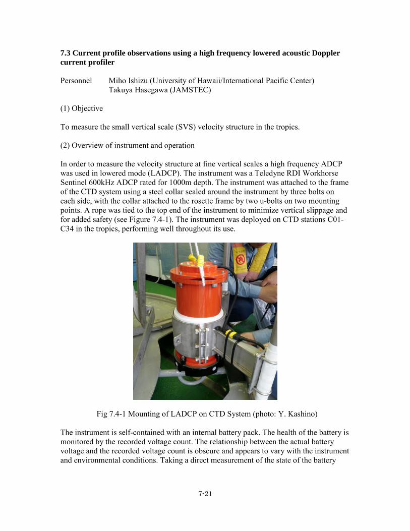
7-21

7.3 Current profile observations using a high frequency lowered acoustic Doppler current profiler Personnel Miho Ishizu (University of Hawaii/International Pacific Center) Takuya Hasegawa (JAMSTEC) (1) Objective To measure the small vertical scale (SVS) velocity structure in the tropics. (2) Overview of instrument and operation In order to measure the velocity structure at fine vertical scales a high frequency ADCP was used in lowered mode (LADCP). The instrument was a Teledyne RDI Workhorse Sentinel 600kHz ADCP rated for 1000m depth. The instrument was attached to the frame of the CTD system using a steel collar sealed around the instrument by three bolts on each side, with the collar attached to the rosette frame by two u-bolts on two mounting points. A rope was tied to the top end of the instrument to minimize vertical slippage and for added safety (see Figure 7.4-1). The instrument was deployed on CTD stations C01-C34 in the tropics, performing well throughout its use.

Fig 7.4-1 Mounting of LADCP on CTD System (photo: Y. Kashino) The instrument is self-contained with an internal battery pack. The health of the battery is monitored by the recorded voltage count. The relationship between the actual battery voltage and the recorded voltage count is obscure and appears to vary with the instrument and environmental conditions. Taking a direct measurement of the state of the battery

7-22

requires opening up the instrument. Direct measurements of the battery voltage were taken before and after the deployment and compared to the recorded voltage count: Battery Voltage (V) Voltage Count (VC) ratio (V/VC) Before 44.82 153 0.29 After 40.60 141 0.29 implying an almost constant relationship of V~=0.29VC. RDI recommends the battery be changed when V gets below 30V. (3) Setup and Parameter settings At all stations the LADCP was controlled at deploy and recover stages by a Linux PC using the python script ladcp600_mr1203.py (written by Eric Firing, University of Hawai`i). The commands sent to the instrument at setup were contained in ladcp600.cmd. The instrument was set up to have a relatively small bin depth (2m) and a fast ping rate (every 0.25 sec). The full list of commands sent to the instrument were:

CR1 # Retrieve parameter (default) TC2 # Ensemble per burst WP1 # Pings per ensemble TE 00:00:00.00 # Time per ensemble (time between data collection cycles) TP 00:00.25 # Time between pings in mm:ss WN25 # Number of Depth cells WS0200 # Depth cell size (in cms) WF0088 # Blank after transit (recommended setting for 600kHz) WB0 # Mode 1 bandwidth control (default - wide) WV250 # Ambiguity velocity (in cm/s) EZ0111101 # Sensor source (speed of sound excluded) EX00000 # Beam coordinates CF11101 # Data flow control parameters (see the RDI Workhorse "Commands and Data Output Format" document for details.) To add flexibility, the instrument could also be controlled at deploy and recover stages by the RDI software (BBTalk) installed on the JAMSTEC Windows PC with the same list of commands as above. In this cruise, we did not have the opportunity to use BBTalk. (4) Data processing An initial sampling of the data was made using the following scripts to check that the instrument was performing correctly make.plots.py integrity check plot pressure, temperature, voltage and current counts

7-23

plot velocity from all 4 beams The principal onboard data processing was performed using the Lamont Doherty Earth Observatory (LDEO, Columbia University) LADCP software package version IX_6beta (available at ftp://ftp/ldeo.columbia.edu/pub/ant/LADCP). The package is based on a number of matlab scripts. The package performs an inverse of the LADCP data, incorporating CTD (for depth) and GPS data, to provide a vertical profile of the horizontal components of velocity, U and V (eastward and northward, respectively), that is a best fit to specified constraints. The down- and up-casts are solved separately, as well as the full cast inverse. The package also calculates U and V from the vertical shear of velocity. The software is run using the matlab script process_cast_mr1203.m with the configuration file set_cast_params.m. Frequent CTD data are required. Files of 1 second averaged CTD data were prepared for each station. Accurate time keeping is also required, particularly between the CTD and GPS data. To ensure this, the CTD data records also included the GPS position. The LDEO software allows the ship’s ADCP data (SADCP) to be included in the inverse calculation. The SADCP data were not included in this case so as to provide an independent check on the functioning of the LADCP. On-station SADCP velocity profiles were produced by averaging the five-minute averaged profiles (mr1203002_000000.LTA and mr1203003_000000.LTA produced using VmDAS) over the period of the CTD/LADCP cast. Care was taken to ensure the average did not contain any spurious data from periods when the ship was maneuvering. (5) Preliminary results

An example of the on-board processed data is presented in Figure 7.3-2 and 7.3-3 compares the full cast inverse, up- and down-cast inverse, and the shear solutions for the zonal (U) and meridional (V) components of the velocity vector with the corresponding SADCP profile for Station C02M01. The LADCP velocity has been fitted to the mean and linear shear of the SADCP velocity. There is a very good correspondence between the general structure of all velocity profiles. While the large vertical scale flow is in a good agreement with the SADCP data (gray line), the LADCP solutions show a lot of smaller scale structure, not resolved by the SADCP. Especially noticeable in Figure 7.3-2 are features in V between 50-300m that are barely resolved by the SADCP.

7-24

Figure 7.3-2 CTD Station C02M01: Vertical profiles of U and V calculated by a number of methods using LADCP data. Full cast inverse (u inverse), downcast only inverse (u_do), up-cast only inverse (u_up) and shear solution (u_shear). Also shown are the profiles using SADCP data (u sadcp). These small vertical scale structures are often associated with small vertical scale anomalies in salinity profiles. As an example, the down- and up-cast inverse solutions for U and V are compared with salinity over a portion of the CTD Station C02_01 profile in Figure 7.3-3. The fact that a number of the same small scale features are evident in both the down- and up- cast profiles of both U and V, confirms the ability of the instrument to measure small vertical scale features in velocity. There is a strong correspondence between the small-scale features in V and salinity and to a smaller extent between U and salinity as well (e.g., slightly above and below the 200 m depth), although the exact relationship will depend on the time evolution of the fields.

7-25

Figure 7.3-3 CTD Station C02M01: Vertical profile of the downcast (green full line) and up-cast (green dashed line) salinity overlain with downcast (red) and up-cast (blue) horizontal velocity components (zonal left panel; meridional right panel). Note the correspondence of salinity with the small vertical scale meridional velocity features. The measurements at individual stations are combined to produce latitudinal and longitudinal sections of the velocity fields. Figures 7.3-4, 7.3-5, 7.3-6 and 7.3-7 show the zonal and meridional components of the velocity vector as a function of latitude and depth at 147E and 156E correspondingly. All plots show the abundance of features with vertical scales 30 – 60 m. Smaller scale features, not evident in the plots shown, are present and resolved by the LADCP. The intensity of such features seems to be independent of latitude. Many SVS features clearly extend over several stations and/or show remarkable spatial correlation. This is particularly evident in contour plots of meridional velocity along latitudinal sections of 147E and 156E. The origin of these features is the subject of an ongoing observational and theoretical investigation. A comparison with the turbulence energy dissipation rate profiles obtained on this cruise using a microstructure profiles (MSP) suggests that these features may account for a significant fraction of the overall dissipation in the thermocline, but further analysis is necessary to quantify their role.

7-26

Figure 7.3-4. Latitudinal section of the zonal component of velocity and potential density at 147E.

Figure 7.3-5. Latitudinal section of the zonal component of velocity and potential density at 156E.

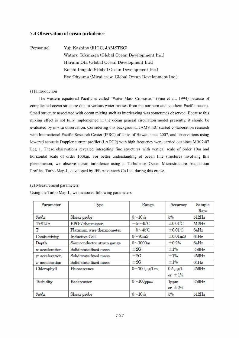
7-27

7.4 Observation of ocean turbulence

Personnel Yuji Kashino (RIGC, JAMSTEC) Wataru Tokunaga (Global Ocean Development Inc.) Harumi Ota (Global Ocean Development Inc.) Koichi Inagaki (Global Ocean Development Inc.) Ryo Ohyama (Mirai crew, Global Ocean Development Inc.) (1) Introduction

The western equatorial Pacific is called “Water Mass Crossroad” (Fine et al., 1994) because of

complicated ocean structure due to various water masses from the northern and southern Pacific oceans.

Small structure associated with ocean mixing such as interleaving was sometimes observed. Because this

mixing effect is not fully implemented in the ocean general circulation model presently, it should be

evaluated by in-situ observation. Considering this background, JAMSTEC started collaboration research

with International Pacific Research Center (IPRC) of Univ. of Hawaii since 2007, and observations using

lowered acoustic Doppler current profiler (LADCP) with high frequency were carried out since MR07-07

Leg 1. These observations revealed interesting fine structures with vertical scale of order 10m and

horizontal scale of order 100km. For better understanding of ocean fine structures involving this

phenomenon, we observe ocean turbulence using a Turbulence Ocean Microstructure Acquisition

Profiles, Turbo Map-L, developed by JFE Advantech Co Ltd. during this cruise.

(2) Measurement parameters

Using the Turbo Map-L, we measured following parameters:

7-28

We use following sensor and twin shear probes:

FP07 sensor

Cast No. 1- 15 SN:219

Cast No. 16-78 SN:220

Shear Ch1 sensor

All casts: SN:718

Shear Ch2 sensor

Cast No. 1- 2 SN:797

Cast No. 3- 8 SN:875

Cast No. 9-78 SN:876

(3) Observation stations.

No. Date Longitude Latitude Logging Time Observation

Depth[m]

File name

(.BIN) Note

Start Stop

01 2012/07/25 146-55.55E 05-03.83N 8:44 9:03 634 MR1203-1 *1 02 2012/07/25 146-55.52E 05-04.12N 9:17 9:34 581 MR1203-2

03 2012/07/26 146-59.91E 04-30.33N 5:17 5:39 725 MR1203-3

04 2012/07/26 146-59.92E 02-05.30N 20:16 20:34 541 MR1203-4

05 2012/07/27 147-00.36E 01-29.84N 5:18 5:39 565 MR1203-5

06 2012/07/27 147-00.20E 00-59.90N 9:15 9:32 545 MR1203-6

07 2012/07/29 147-00.38E 00-29.84N 9:10 9:28 524 MR1203-7

08 2012/07/29 147-02.12E 00-01.53N 20:03 20:22 613 MR1203-8

09 2012/08/03 156-00.12E 03-30.27S 7:56 8:14 574 MR1203-9

10 2012/08/04 156-02.38E 04-58.78S 2:48 3:06 628 MR1203-10

11 2012/08/04 156-00.17E 04-30.20S 7:10 7:27 556 MR1203-11

12 2012/08/05 156-00.20E 04-00.35S 5:49 6:04 528 MR1203-12

13 2012/08/08 156-00.51E 02-00.92S 19:21 19:41 632 MR1203-13

14 2012/08/09 156-00.06E 02-30.06S 3:02 3:19 585 MR1203-14

15 2012/08/09 156-00.07E 03-00.06S 6:58 7:16 581 MR1203-15 *2 16 2012/08/09 156-00.26E 03-00.15S 7:49 8:06 578 MR1203-16

17 2012/08/10 156-00.05E 01-30.28S 5:01 5:17 555 MR1203-17

18 2012/08/10 156-00.14E 01-00.18S 9:05 9:22 569 MR1203-18

19 2012/08/12 156-00.36E 00-30.28S 6:57 7:15 597 MR1203-19

20 2012/08/12 156-00.18E 00-00.03N 19:33 19:52 535 MR1203-20

21 2012/08/12 156-00.69E 00-00.21N 20:09 20:28 543 MR1203-21

22 2012/08/12 156-00.94E 00-00.42N 20:45 21:04 588 MR1203-22

23 2012/08/12 156-00.84E 00-00.09N 22:31 22:50 568 MR1203-23

7-29

24 2012/08/12 156-01.13E 00-00.22N 23:06 23:23 568 MR1203-24

25 2012/08/12 156-01.45E 00-00.34N 23:39 23:57 606 MR1203-25

26 2012/08/13 155-59.76E 00-00.09N 1:27 1:46 523 MR1203-26

27 2012/08/13 155-59.98E 00-00.24N 2:04 2:22 575 MR1203-27

28 2012/08/13 156-00.09E 00-00.39N 2:39 2:56 535 MR1203-28

29 2012/08/13 156-00.14E 00-00.28N 4:27 4:46 552 MR1203-29

30 2012/08/13 156-00.21E 00-00.55N 5:06 5:24 560 MR1203-30

31 2012/08/13 156-00.32E 00-00.63N 5:41 6:00 573 MR1203-31

32 2012/08/13 156-00.14E 00-00.00N 7:30 7:48 544 MR1203-32

33 2012/08/13 156-00.25E 00-00.03N 8:03 8:20 567 MR1203-33

34 2012/08/13 156-00.43E 00-00.12N 8:34 8:52 574 MR1203-34

35 2012/08/13 156-00.05E 00-00.12S 10:29 10:46 527 MR1203-35

36 2012/08/13 156-00.62E 00-00.06S 11:04 11:22 558 MR1203-36

37 2012/08/13 156-01.20E 00-00.02S 11:38 11:54 529 MR1203-37

38 2012/08/13 155-59.62E 00-00.17N 13:27 13:45 511 MR1203-38

39 2012/08/13 156-00.13E 00-00.26N 14:00 14:17 532 MR1203-39

40 2012/08/13 156-00.56E 00-00.32N 14:32 14:50 563 MR1203-40

41 2012/08/13 155-59.42E 00-00.21S 16:27 16:45 552 MR1203-41

42 2012/08/13 155-59.79E 00-00.11S 16:58 17:16 551 MR1203-42

43 2012/08/13 156-00.13E 00-00.02N 17:29 17:49 594 MR1203-43

44 2012/08/13 155-59.68E 00-00.18S 19:29 19:49 593 MR1203-44

45 2012/08/13 155-59.93E 00-00.06S 20:06 20:24 572 MR1203-45

46 2012/08/13 156-00.15E 00-00.07N 20:40 20:59 584 MR1203-46

47 2012/08/13 156-00.16E 00-15.07N 23:23 23:42 551 MR1203-47

48 2012/08/13 156-00.25E 00-15.13N 23:57 0:14 568 MR1203-48

49 2012/08/14 156-00.32E 00-15.18N 0:31 0:48 552 MR1203-49

50 2012/08/14 156-00.13E 00-30.12N 3:11 3:27 519 MR1203-50

51 2012/08/14 156-00.19E 00-30.28N 3:43 3:58 525 MR1203-51

52 2012/08/14 156-00.24E 00-30.39N 4:13 4:30 521 MR1203-52 *3 53 2012/08/14 156-00.29E 00-30.47N 4:46 5:03 536 MR1203-53

54 2012/08/14 156-00.22E 00-45.27N 7:19 7:36 533 MR1203-54

55 2012/08/14 156-00.22E 00-45.35N 7:49 8:05 529 MR1203-55

56 2012/08/14 156-00.23E 00-45.44N 8:18 8:36 541 MR1203-56

57 2012/08/14 156-00.24E 01-00.34N 10:49 11:05 544 MR1203-57

58 2012/08/14 156-00.47E 01-00.65N 11:19 11:35 544 MR1203-58

59 2012/08/14 156-00.70E 01-00.98N 11:51 12:05 528 MR1203-59

60 2012/08/14 156-00.13E 01-15.09N 14:10 14:27 535 MR1203-60

7-30

61 2012/08/14 156-00.32E 01-15.37N 14:40 14:57 550 MR1203-61

62 2012/08/14 156-00.55E 01-15.65N 15:09 15:25 538 MR1203-62

63 2012/08/14 156-02.80E 01-30.41N 17:43 17:59 516 MR1203-63

64 2012/08/14 156-03.00E 01-30.84N 18:14 18:30 527 MR1203-64

65 2012/08/14 156-03.17E 01-31.21N 18:44 18:59 524 MR1203-65

66 2012/08/14 156-00.35E 01-45.41N 21:10 21:29 628 MR1203-66

67 2012/08/14 156-00.44E 01-45.55N 21:45 22:03 613 MR1203-67

68 2012/08/14 156-00.52E 01-45.74N 22:22 22:41 596 MR1203-68

69 2012/08/15 156-01.67E 01-57.68N 0:47 1:07 602 MR1203-69

70 2012/08/15 156-01.70E 01-57.90N 1:20 1:37 583 MR1203-70

71 2012/08/15 156-01.74E 01-58.14N 1:50 2:07 578 MR1203-71

72 2012/08/15 156-00.23E 02-30.21N 5:44 6:01 606 MR1203-72

73 2012/08/16 156-00.16E 03-00.07N 7:00 7:17 595 MR1203-73

74 2012/08/17 156-00.15E 03-30.14N 8:17 8:36 660 MR1203-74

75 2012/08/17 155-59.33E 05-01.02N 19:09 19:27 645 MR1203-75

76 2012/08/18 156-02.79E 04-29.92N 4:19 4:37 585 MR1203-76

77 2012/08/18 156-00.09E 03-59.97N 8:19 8:36 562 MR1203-77

78 2012/08/19 156-00.71E 07-58.63N 19:13 19:31 600 MR1203-78

*1) Because we found spike noise in vertical acceleration in this cast, we carried out the second cast.

*2) Because data from FP07 sensor was bad in this cast, we carried out the second cast after FP07 sensor

was exchanged.

*3) Because we found large shear around the depths of 410m and 460m in this cast, we conducted an

additional cast.

During this cruise, we conducted following special observations for better understanding the fine

structure and its daily variability:

a) 24-hours observation at the equator, 156E (every 3 hours)

b) Observations with meridional interval of 15 nautical miles between 2N and equator along 156E

During both observations, 3 cast were carried out at each time.

7-31

(4) Operation and data processing

We operated the Turbo Map-L by a crane which is usually used for foods supply and installed in the

middle of ship. We lowered it at the starboard of R/V Mirai (Photo 7-4-1).

Photo 7-4-1. Observation using Turbo Map-L.

Measurement depth was 500m because our interest is ocean turbulence around thermocline. Descent

rate of the Turbo Map-L was 0.5 – 0.7 m s-1.

Data acquisition and processing were carried out using a PC in the Atmospheric Gas Observation

Room of R/V Mirai (Photo 7-4-2). Data processing software was TM-Tool ver 3.04D provided by JFE

Advantech Co Ltd.

Photo 7-4-2. Data acquisition and processing in the Atmospheric Gas Observation Room.

7-32

5) Results

Figure 7-4-1 shows the sections of logarithm of energy dissipation rate (epsilon) along 147E, and

156E. Compared with salinity section (Figure 2-2), there are following tendencies:

a) High epsilon was generally seen in the high salinity water exceeding 35 PSU (100-200m).

b) There is minimum layer of epsilon below 200m depth.

These results suggest that ocean mixing is active around high salinity water exceeding 35 PSU (South

Pacific Tropical Water).

Figure 7-4-1. Vertical section of logarithm of energy dissipation rate along a) and

b) 156E during MR12-03 cruise.

a)

b)

7-33

7.5 Argo floats 7.5.1 Profiling floats for JAMSTEC Argo Project (1) Personnel

Toshio Suga (JAMSTEC/RIGC): Principal Investigator (not on board) Shigeki Hosoda (JAMSTEC/RIGC): not on board Kanako Sato (JAMSTEC/RIGC): not on board Mizue Hirano (JAMSTEC/RIGC): not on board Hiroki Ushiromura (MWJ): Technical Staff (Operation Leader)

(2) Objectives

The objective of deployment is to clarify the structure and temporal/spatial variability of water masses in the North Pacific such as North Pacific Tropical Water in the subtropical North Pacific.

The profiling floats launched in this cruise measure vertical profiles of temperature and salinity automatically every ten days. As the vertical resolution of the profiles is very fine, the structure and variability of the water mass can be displayed well. Therefore, the profile data from the floats will enable us to understand the variability and the formation mechanism of the water mass.

(3) Parameters

・water temperature, salinity, and pressure (4) Methods

i. Profiling float deployment

We launched an Arvor float manufactured by nke. These floats equip an SBE41cp CTD sensor manufactured by Sea-Bird Electronics Inc.

The floats usually drift at a depth of 1000 dbar (called the parking depth), diving to a depth of 2000 dbar and rising up to the sea surface by decreasing and increasing their volume and thus changing the buoyancy in ten-day cycles. During the ascent, they measure temperature, salinity, and pressure. They stay at the sea surface for approximately nine hours, transmitting the CTD data to the land via the ARGOS system, and then return to the parking depth by decreasing volume. The status of floats and their launches are shown in Table 7.5.1-1.

7-34

Table 7.5.1-1 Status of floats and their launches Float(2000dbar)

Float Type Arvor float manufactured by nke. CTD sensor SBE41cp manufactured by Sea-Bird Electronics Inc.

Cycle 10 days (approximately 9 hours at the sea surface) ARGOS transmit interval 30 sec Target Parking Pressure 1000 dbar

Sampling layers 115 (2000,1950,1900,1850,1800,1750,1700,1650,1600,1550,1500, 1450, 1400, 1350, 1300, 1250, 1200, 1150, 1100, 1050, 1000, 980,

960, 940, 920, 900, 880, 860, 840, 820, 800, 780, 760, 740, 720, 700, 680, 660, 640, 620, 600, 580, 560, 540, 520, 500, 490, 480, 470, 460, 450, 440, 430, 420, 410, 400, 390, 380, 370, 360, 350, 340, 330, 320, 310, 300, 290, 280, 270, 260, 250, 240, 230, 220,210, 200, 195, 190, 185, 180, 175, 170, 165, 160, 155, 150, 145, 140, 135, 130, 125, 120, 115, 110, 105, 100, 95, 90, 85, 80, 75, 70, 65, 60, 55, 50, 45, 40, 35,

30, 25, 20, 15, 10, 4 or surface dbar)

Launches Float S/N

ARGOS ID

Date and Time of Reset (UTC)

Date and Time of Launch(UTC)

Location of Launch

CTD St. No.

11009 112238 2012/08/21 22:50

2012/08/21 23:56

12-00.29N 154-18.12E

C35

(5) Data archive

The real-time data are provided to meteorological organizations, research institutes, and

universities via Global Data Assembly Center (GDAC: http://www.usgodae.org/argo/argo.html, http://www.coriolis.eu.org/) and Global Telecommunication System (GTS), and utilized for analysis and forecasts of sea conditions.

Fig. 7.5.1-1. The profile of the float launched during MR12-03.

7-35

7.5.2 ARGO float mission off Papua New Guinea

(1) Personal

(a) On board

Takuya Hasegawa (JAMSTEC/RIGC: Principal Investigator for this mission)

Hiroki Ushiromura (MWJ: Chief technical staff of MR12-03 for this mission)

Rei Ito (MWJ)

Kazuma Takahashi (MWJ)

(b) Not on board

Toshio Suga (JAMSTEC/RIGC)

Shigeki Hosoda (JAMSTEC/RIGC)

Kanako Sato (JAMSTEC/RIGC)

Mizue Hirano (JAMSTEC/RIGC)

Hiroyuki Nakajima (MWJ)

Kentaro Ando (JAMSTEC/RIGC)

Takanori Horii (JAMSTEC/RIGC)

Yoshimu Kusumoto (Hydro System development Inc)

(2) Outline and objectives

One Argo float (Navigation European Marine Observer: NEMO: Fig.7.5.2-1) was

launched off Papua New Guinea (2.72S-153.27E, near subsurface-ADCP moorings

deployment points; see Fig.7.5.2-2) on 1st August 2012 (UTC) as a part of

CLIVAR-SPICE related observations during MR12-03.

The purpose of this NEMO float mission is to obtain one temperature and salinity

profile per one day in order to merge the data with current velocity observed by two

subsurface-ADCP moorings deployed at around 2.7S-153E to explore temperature and

salinity transport of the New Ireland Coastal Undercurrent (NICU), which is suggested

to be important for Pacific warm water pool changes by recent studies.

For this purpose, mission parameters of this NEMO float were highly tuned to make the

float stay near the ADCP moorings deployment points (see subsection (4)). In addition,

MTMs (Mobile Terminated Messages), which can change the mission parameters of

7-36

NEMO float after its launch via Iridium communication, can be automatically made

using mission-control-programs that were specially made for this mission at Argo float.

The MTMs to the NEMO float are automatically sent via Iridium communication server

from Argo-float data server at Yokosuka HQ of JAMSTEC using these programs at

06:00 (UTC) everyday. The contents of MTMs (e.g., parking depth) are decided by the

programs by use of information of MOMs (Mobile Originated Messages; those are

emitted from the NEMO float using Iridium communication and include information

concerning position of NEMO float, observed temperature and other data, and technical

information of the NEMO float). The MTMs can be made and sent by manual operation

in addition to the automatic operation using the mission-control-programs.

As described above, this NEMO-float mission focuses on water properties of NICU off

Papua New Guinea. After the NEMO float will go out from the NICU area, its mission

will be changed to that of standard Argo floats with 10-day observation cycle by using

MTMs.

(3) Parameters

Water temperature, salinity and pressure

(4) Methods and float information

(a) Type of the float: NEMO float, manufactured by Optimare Ltd.

(b) Serial number of the NEMO float: 222

(c) Iridium communication number (IMEI): 300234011420390

(d) Date and time of launch (UTC): 2012/08/01 05:29

(e) Location of launch: 2.72S-153.27E

(f) Main sensor: SBE41CP CTD sensor, manufactured by Sea-Bird Electonics Inc.

(g) Transmission system: Iridium communication (SBD type)

(h) Mission cycle time: 1440 minutes (nearly 30 minutes at the sea surface)

(i) Startup delay: 1380 minutes (23:00 UTC)

(j) Startup time: 480 minutes

(k) Maximum transmission time at sea surface: 60 minutes

(l) Observing layer: from surface to 650 dbar with continuous mode (1 Hz sampling)

(m) CTD pressure sample interval during descent: 10 seconds

7-37

(n) Target parking pressure: 550 dbar near launching point

(o) Ascent speed and mode: 0.10 m/s with controlled mode

(p) Descent speed and mode: 0.08 m/s with controlled mode

(q) Seg speed: 0.08 m/s

(r) CTD sample interval at parking pressure: 1440 minutes

Mission parameters related to parking depth, mission cycle time, ascent speeds,

observation layer etc. can be changed after launch by MTMs using Iridium

communication.

(5) Data archive

The real-time data are provided to meteorological organizations, research institutes,

and universities via Global Data Assembly Center (GDAC:

http://www.usgodae.org/argo/argo.html, http://www.coriolis.eu.org/) and Global

Telecommunication System (GTS), and utilized for analysis and forecasts of sea

conditions.

Fig

ure 7.5.2-1: NEMO float just after and before its launch (left and right, respectively).

Figure 7.5.2-2: Location of launch of the

NEMO float (2.72S-153.27E: shown by a

green cross mark). Current velocities for

NICU layer from high-resolution ocean

general circulation model (OFES)

simulation are also shown by black arrows

(unit in cm/s).

NICU

Papua New Guinea

7-38

7.6 Global Drifter Program – SVP Drifting Buoys (1) Personnel

Rick Lumpkin (National Oceanographic Atmospheric Administration / Global Drifter Program): Principal Investigator of GDP (not on board)

Shaun Dolk (National Oceanographic Atmospheric Administration / Global Drifter Program): (not on board)

(2) Objectives

The objective of deploying the 20 drifting buoys is to compliment the current global array of drifting buoys. The western equatorial region is of great value, as there are few deployment opportunities in this region. As a result, the data collected from these instruments will significantly affect the current dataset of historical drifters in the area.

(3) Parameters

Sea surface temperature and ocean current velocities.

(4) Methods

i. Profiling float deployment

We launched ten (10) drifting buoys manufactured by Clearwater Instruments and ten (10) drifters manufactured by Data Buoy instrumentation. These drifters are equipped with thermistor sensors to measure the temperature at the surface of the ocean. The drifters float at the surface, following upper ocean surface currents. The measured temperature and location data are sent to the Drifter Data Assembly Center via the ARGOS transmitting system for data processing and quality control procedures. The drifters are expected to transmit for 450 days, while maintaining a drogue presence for 300 days. The status of drifters and their launches are shown in Table 7.6.1.

7-39

Table 7.6.1 Status of drifters and their launches Drifter Type Surface Velocity Profiler (SVP) Type drifter Manufactured

by Clearwater and DBi. Launches

(5) Data archive

The real time data are provided via DAC Data Products, which you can access at (http://www.aoml.noaa.gov/phod/dac/meds.html). The quality controlled data are provided to oceanographic organizations, research institutes, and universities via Drifter Data Assembly Center (http://www.aoml.noaa.gov/phod/dac/dirall.html) and Global Telecommunication System (GTS), and utilized for analysis and forecasts of the ocean conditions and the climates.

7-40

7.7 Radiosonde observation for the validation of GOSAT and ship-borne sky radiometer products Shuji KAWAKAMI (JAXA EORC, PI) Kazuma AOKI (Toyama University, PI/not on board) Tadahiro HAYASAKA (Tohoku University, not on board) Yoshimi KAWAI (JAMSTEC RIGC, not on board) Wataru TOKUNAGA (GODI) Harumi OHTA (GODI) Kouichi INAGAKI (GODI) (1) Objective

We performed the radiosonde observations to obtain vertical profiles of temperature and water vapor for the validation of GOSAT and ship-borne sky radiometer products, and to investigate atmospheric and cloud structure responding to the ocean temperature front of the Kuroshio Extension.

(2) Parameters

According to the manufacturer, the range and accuracy of parameters measured by the radiosonde sensor (RS92-SGP) are as follows;

Parameter Range Accuracy Pressure 3~1080 hPa +/- 1 hPa (1080-100 hPa), +/- 0.6 hPa (100-3 hPa) Temperature -90~60 °C +/- 0.5 °C Humidity 0~100 % 5 %

(3) Method

Atmospheric soundings by radiosondes were performed in the western Pacific Ocean. In total, 45 soundings were carried out, but note that one sounding (RS37) stopped at only 6569 m height (Table 7.7-1, Figure 7.7-1). The main system consisted of processor (Vaisala, DigiCORA III MW31), GPS antenna (GA20), UHF antenna (RB21), ground check kit (GC25), balloon launcher (ASAP), and GPS radiosonde sensor (RS92-SGP).


Precipitable water calculated from the sounding data is shown in Figures 7.7-2. Note that it was derived from the surface to the middle troposphere for RS37. The Kuroshio Extension region became quite humid after the Baiu season, and the precipitable water in this region was close to that in the tropics.

(5) Data archive

Raw data were recorded in ASCII format every 2 seconds during ascent. These raw data were submitted to the Data Management Group of JAMSTEC just after the cruise.

7-41

Table 7.7-1. Radiosonde launch log. Sounding

No. Launching Maximum Duration

(sec) Date (UT) Lon Lat Altitude hPa RS01 2012/07/17 20:34:43 37.846 142.758 20287 55.3 5224 RS02 2012/07/18 02:34:34 36.729 143.036 22700 37.9 6424 RS03 2012/07/18 08:31:16 35.748 143.257 21902 42.8 4542 RS04 2012/07/18 14:30:34 34.707 143.517 23008 35.7 5484 RS05 2012/07/18 20:30:27 33.603 143.765 22953 35.9 5352 RS06 2012/07/20 03:01:03 27.621 144.896 23035 35.1 5208 RS07 2012/07/21 14:10:15 20.871 146.088 21777 42.3 5492 RS08 2012/07/23 03:10:24 13.640 146.665 24690 26.3 5942 RS09 2012/07/24 14:25:36 6.791 146.794 23021 34.1 5646 RS10 2012/07/25 02:41:49 4.972 146.971 22927 34.6 5068 RS11 2012/07/27 14:25:21 1.535 146.974 20365 52.3 6474 RS12 2012/07/28 02:40:44 2.084 146.964 23337 32.3 5244 RS13 2012/07/30 14:24:47 -0.100 149.160 17370 86.8 2916 RS14 2012/07/31 02:40:06 -0.209 150.538 21303 44.8 5392 RS15 2012/08/02 02:11:17 -3.273 153.069 24271 27.9 6380 RS16 2012/08/02 14:25:24 -4.868 154.249 22476 37.0 5712 RS17 2012/08/05 02:12:18 -4.584 156.001 23578 31.2 6312 RS18 2012/08/05 14:25:09 -4.265 157.004 20772 49.0 6284 RS19 2012/08/07 15:10:10 -4.784 157.589 22198 38.9 5384 RS20 2012/08/08 02:10:05 -4.275 157.394 24896 25.2 6310 RS21 2012/08/08 14:25:22 -2.716 156.444 23409 31.9 6012 RS22 2012/08/10 03:09:46 -1.786 155.979 23495 31.4 5950 RS23 2012/08/10 13:50:17 -0.593 156.017 22632 36.1 6082 RS24 2012/08/11 00:10:13 -0.019 156.095 22934 34.5 5372 RS25 2012/08/11 02:09:43 -0.040 156.141 23132 33.3 5538 RS26 2012/08/11 04:11:15 -0.046 156.063 19712 58.4 4626 RS27 2012/08/12 03:10:13 -0.037 156.133 20040 55.1 5432 RS28 2012/08/12 15:30:49 -0.001 155.976 21245 45.2 5108 RS29 2012/08/13 13:50:04 0.003 155.992 22607 36.3 5514 RS30 2012/08/14 02:09:59 0.361 156.003 24429 27.1 6360 RS31 2012/08/14 14:26:35 1.250 156.001 22148 38.9 5128 RS32 2012/08/16 13:51:17 2.410 156.083 23308 32.5 6092 RS33 2012/08/17 02:11:42 2.379 156.018 23909 29.5 5512 RS34 2012/08/19 03:10:14 5.254 155.992 24060 29.0 6026 RS35 2012/08/19 13:55:14 7.262 155.999 22979 34.3 5814 RS36 2012/08/20 02:10:51 7.970 156.022 21334 44.7 5228 RS37 2012/08/22 13:57:27 14.583 153.183 6569 457.2 1308 RS38 2012/08/23 14:31:27 18.185 151.593 23319 32.9 5910 RS39 2012/08/24 02:35:24 20.524 150.663 22418 38.0 5486

7-42

RS40 2012/08/25 03:04:56 25.431 148.658 20283 54.2 5288 RS41 2012/08/26 14:31:01 32.652 145.552 22658 37.5 5696 RS42 2012/08/26 20:29:51 33.812 145.029 23827 31.4 6184 RS43 2012/08/27 02:30:09 34.914 144.525 23758 31.7 5920 RS44 2012/08/27 08:30:08 36.080 143.994 24003 30.8 6298 RS45 2012/08/27 14:30:17 37.251 143.437 22434 39.3 5546

Figure 7.7-1. Positions of the GPS radiosonde (dots).

7-43

Figure 7.7-2. Precipitable water for (upper) each sounding number and (lower) latitude.

7-44

7.8 Validation of GOSAT products over sea using a ship-borne compact system for measuring atmospheric trace gas column densities Shuji KAWAKAMI (JAXA EORC) Hirofumi OHYAMA (JAXA SAPC) (1) Objective Greenhouse gases Observing SATellite (GOSAT) was launched on 23 January 2009 in order to monitor the global distributions of atmospheric greenhouse gas concentrations: column-averaged dry-air mole fractions of carbon dioxide (CO2) and methane (CH4). A network of ground-based high-resolution Fourier transform spectrometers provides essential validation data for GOSAT. Vertical CO2 profiles obtained during ascents and descents of commercial airliners equipped with the in-situ CO2 measuring instrument are also used for the GOSAT validation. Because such validation data are obtained mainly over land, there are very few data available for the validation of the over-sea GOSAT products. The objectives of our research are to acquire the validation data over sea using an automated compact instrument and to compare the acquired data with the over-sea GOSAT products. (2) Description of instruments deployed The column-averaged dry-air mole fractions of CO2 and CH4 can be estimated from absorption by atmospheric CO2 and CH4 that is observed in a solar spectrum. An optical spectrum analyzer (OSA, Yokogawa M&I co., AQ6370) was used for measuring the solar absorption spectra in the near-infrared spectral region. A solar tracker (PREDE co., ltd.) and a small telescope (Figure 7.8-1) collected the sunlight into the optical fiber that was connected to the OSA. The solar tracker searches the sun every one minute until the sunlight with a defined intensity is detected. The measurements of the solar spectra were performed during solar zenith angles of <80°. In addition, radiosonde observations, which were collocated with the GOSAT overpass time (both daytime and nighttime), were made to obtain vertical profiles of atmospheric temperature and humidity. (3) Analysis method

The CO2 absorption spectrum at the 1.6 µm band measured with the OSA is shown in Figure 2. The absorption spectrum can be simulated based on radiative transfer theory using assumed atmospheric profiles of pressure, temperature, and trace gas concentrations. The column abundance of CO2 (CH4) was retrieved by adjusting the assumed CO2 (CH4) profile to

Figure 7.8-1. Solar tracker and telescope. The sunlight collected into optical fiber was introduced into the OSA that was installed in an observation room in the MIRAI.

7-45

minimize the differences between the measured and simulated spectra. Figure 3 shows an example of spectral fit performed for the spectral region with the CO2 absorption lines. The column-averaged dry-air mole fraction of CO2 (CH4) was obtained by taking the ratio of the CO2 (CH4) column to the dry-air column.


The observations were made from July 17 to August 29 continuously in daytime including while the ship was at the Sekinehama sea-port (Table 7.8-1 and Figure 7.8-1). Radiosonde data were obtained at the GOSAT overpass in daytime (Table 7.8-1).

Figure 7.8-2. 1.6 µm CO2 absorption spectrum measured with the OSA.

Figure 7.8-3. Spectral fit performed for the 6297–6382 cm−1 region using an OSA spectrum. Open diamonds denote the measured spectrum, and the solid line denotes the spectrum calculated from the retrieval result. The residual between the measured and calculated spectra is also shown.

7-46

Date Time(JST)Time(JST)

Latitude(degN)

Longitude(degE)

2012/07/17 7:25-18:002012/07/18 7:02-10:152012/07/19 7:24-17:522012/07/20 6:34-18:00 12:00 27.621 144.8962012/07/21 5:02-17:092012/07/22 5:42-10:032012/07/23 7:02-16:34 12:10 13.640 146.6652012/07/24 5:44-17:002012/07/25 10:36-15:24 11:55 4.972 146.9712012/07/26 6:13-11:292012/07/27 5:51-13:022012/07/28 -- 11:40 2.084 146.9642012/07/29 --2012/07/30 9:55-17:582012/07/31 8:03-16:29 11:40 -3.273 153.0692012/08/01 5:45-16:512012/08/02 5:18-16:55 11:10 -3.273 153.0692012/08/03 6:14-16:302012/08/04 5:18-16:412012/08/05 5:22-12:52 11:10 -4.584 156.0012012/08/06 5:22-13:532012/08/07 5:24-16:512012/08/08 5:23-16:05 11:10 -4.275 157.3942012/08/09 6:56-16:112012/08/10 5:12-12:522012/08/11 5:06-16:00 11:10 -0.040 156.1412012/08/12 6:05-13:482012/08/13 5:41-11:482012/08/14 5:24-16:01 11:10 0.361 156.0032012/08/15 5:26-15:482012/08/16 --2012/08/17 5:27-16:05 11:10 2.379 156.0182012/08/18 5:08-16:042012/08/19 5:18-16:022012/08/20 5:21-16:41 11:10 5.254 155.9922012/08/21 6:31-15:512012/08/22 5:19-12:002012/08/23 6:49-14:312012/08/24 5:25-16:34 11:35 20.524 150.6632012/08/25 5:25-16:59 12:05 25.431 148.6582012/08/26 5:34-16:592012/08/27 5:34-15:242012/08/28 5:57-17:412012/08/29 6:17-10:19

Radiosonde at the GOSAToverpass in daytime

CO2 observations

-10

0

10

20

30

40

50

140 145 150 155 160

Locations of CO2 observations

Latitu

de

Longitude Table 7.8-1. Period of CO2 observations and Radiosonde Figure 7.8-1. Locations of CO2 observations (5) Data archive The column-averaged dry-air mole fractions of CO2 and CH4 retrieved from the OSA spectra will be submitted to JAMSTEC Data Integration and Analyses Group (DIAG).

7-47

7.9 Lidar observations of clouds and aerosols Nobuo SUGIMOTO (NIES) Ichiro MATSUI (NIES) Atsushi SHIMIZU (NIES) Tomoaki NISHIZAWA (NIES) Hajime OKAMOTO (Kyusyu university)

(Lidar operation was supported by Global Ocean Development Inc. (GODI).) (1) Objectives

Objectives of the observations in this cruise is to study distribution and optical characteristics of ice/water clouds and marine aerosols using a two-wavelength polarization Mie lidar. (2) Description of instruments deployed

Vertical profiles of aerosols and clouds are measured with a two-wavelength polarization Mie lidar. The lidar employs a Nd:YAG laser as a light source which generates the fundamental output at 1064nm and the second harmonic at 532nm. Transmitted laser energy is typically 30mJ per pulse at both of 1064 and 532nm. The pulse repetition rate is 10Hz. The receiver telescope has a diameter of 20 cm. The receiver has three detection channels to receive the lidar signals at 1064 nm and the parallel and perpendicular polarization components at 532nm. An analog-mode avalanche photo diode (APD) is used as a detector for 1064nm, and photomultiplier tubes (PMTs) are used for 532 nm. The detected signals are recorded with a transient recorder and stored on a hard disk with a computer. The lidar system was installed in a container which has a glass window on the roof, and the lidar was operated continuously regardless of weather. Every 10 minutes vertical profiles of four channels (532 parallel, 532 perpendicular, 1064, 532 near range) are recorded. (3) Preliminary results

The two wavelength polarization Mie lidar worked well and succeeded in getting the lidar data during the observation period from July 17 to Aug. 29, 2012.

Examples of the measured data are depicted in Fig. 7.9-1. The figures indicates that the lidar can detect aerosols in the planetary boundary layer (PBL) formed below 1km, water clouds formed at the top of the PBL, ice clouds in the upper layer. It should be noted that the lidar could detect ice clouds (cirrus) up to very high altitude of 16km since optical and microphysical properties and distributions of cirrus are key parameters for evaluating climate change. The figure also depicts that the lidar signals in the PBL are larger on Aug. 7 than on Aug. 6 and Aug. 8, implying that the aerosol concentration and/or their optical properties changes. The measured depolarization ratios in the three days are low, indicating that the spherical aerosols (e.g., sulfate, nitrate, organic carbon, and sea-salt particles) are rich. Combined analysis of the spectral ratio of lidar signals, surface wind speed, relative humidity and observation area data are effective in order to understand this phenomena better.

7-48

Figure 7.9-1: Time-height sections of backscatter intensities at 532nm and 1064nm and total depolarization ratios at 532nm measured from Aug. 6 to Aug. 8, 2012. (4) Data archive - Raw data temporal resolution 10min / vertical resolution 6 m data period (UTC): July. 17, 2012 – Aug. 29, 2012 lidar signal at 532 nm, lidar signal at 1064 nm, depolarization ratio at 532 nm - Processed data (plan) cloud base height, apparent cloud top height, phase of clouds (ice/water), cloud fraction boundary layer height (aerosol layer upper boundary height), backscatter coefficient of aerosols, particle depolarization ratio of aerosols * Data policy and Citation Contact NIES lidar team (nsugimot/i-matsui/shimizua/[email protected]) to utilize lidar data for productive use.

7-49

7.10 Aerosol optical characteristics measured by Shipborne Sky radiometer

Kazuma Aoki (University of Toyama) Principal Investigator / not onboard Tadahiro Hayasaka (Tohoku University) Co-worker / not onboard

(1) Objective

Objective of the observations in this aerosol is to study distribution and optical characteristics of marine aerosols by using a ship-borne sky radiometer (POM-01 MKII: PREDE Co. Ltd., Japan). Furthermore, collections of the data for calibration and validation to the remote sensing data were performed simultaneously.

(2) Methods and Instruments

Sky radiometer is measuring the direct solar irradiance and the solar aureole radiance distribution, has seven interference filters (0.34, 0.4, 0.5, 0.675, 0.87, 0.94, and 1.02 µm). Analysis of these data is performed by SKYRAD.pack version 4.2 developed by Nakajima et al. 1996. @ Measured parameters

- Aerosol optical thickness at five wavelengths (400, 500, 675, 870 and 1020 nm) - Ångström exponent - Single scattering albedo at five wavelengths - Size distribution of volume (0.01 µm – 20 µm)

# GPS provides the position with longitude and latitude and heading direction of the vessel, and azimuth and elevation angle of sun. Horizon sensor provides rolling and pitching angles.


This study is not onboard. Data obtained in this cruise will be analyzed at University of Toyama. (4) Data archives

Measurements of aerosol optical data are not archived so soon and developed, examined, arranged and finally provided as available data after certain duration. All data will archived at University of Toyama (K.Aoki, SKYNET/SKY: http://skyrad.sci.u-toyama.ac.jp/) after the quality check and submitted to JAMSTEC.

7-50

7.11 Continuous measurement of the water stable isotopes over the Ocean (1) Personnel Yasushi Fujiyoshi (Hokkaido Univ./JAMSTEC) Principal Investigator（not on-board） Naoyuki Kurita (JAMSTEC)

Operator Wataru Tokunaga, Harumi Ota, Kouichi Inagaki (Global Ocean Development Inc.: GODI) Ryo Ohyama (MIRAI Crew)

(2) Objective It is well known that the variability of stable water isotopes (HDO and H2

18O) reflects the integrated history of water mass exchange that occurs during transportation from the upstream region. Thus, water isotope tracer is recognized as the powerful tool to study of the hydrological cycles in the marine atmosphere. However, oceanic region is one of sparse region of the isotope data, it is necessary to fill the data to identify the moisture sources by using the isotope tracer. In this study, to fill this sparse observation area, intense water isotopes observation was conducted along the cruise track of MR12-03. (3) Method

Following observation was carried out throughout this cruise. - Atmospheric moisture sampling:

Water vapor isotopes in ambient air was continuously measured using the laser instrument based on off-axis integrated cavity output spectroscopy, manufactured by Los Gatos Research, Inc. (LGR) (Water Vapor Iso- tope Analyzer, WVIA) coupled with an accessory device for the vaporization of a liquid water standard (Water Vapor Isotope Standard Source, WVISS). The WVISS is programmable from the WVIA and thus this coupled system is capable of automatically conducting a calibration routine at specific intervals.

Air intake was attached at the middle level (20m above the sea level) of the mast at the compass deck and a sampling tube (20 m length of Nylon tubing (Junron A), 8mm O.D.) was connected from air intake to a 3-way valve attached to the WVISS. A 1.0 μm filter with PTFE membrane was placed where the tube enters the air intake. Air was drawn via the pump at a flow rate of 3 l min-1 to the laboratory and then a part of air was sacked via the WVIA external pump at a flow rate of 0.5 l min−1. Every 25 min, the 3-way valve automatically switched from ambient/outdoor inlet to WVISS standard air, whereupon standard air with a H2O concentration of 12 000 ppm was introduced to the WVIA for 5 min. After finishing the reference gas measurement, the valve switches back and ambient air sampling is resumed. Raw data from the analyzer is stored on the internal hard disk, and is transferred via ethernet cable. Calibration is undertaken as a post-processing step using the external computer system.

- Rainwater sampling

Rainwater samples gathered in rain/snow collector were collected just after precipitation events have ended. The collected sample was then transferred into glass bottle (6ml) immediately after the measurement of precipitation amount.

- Surface seawater sampling

7-51

Seawater sample taken by the pump from 4m depths were collected in glass bottle (6ml) around the noon at the local time.

(4) Water samples for isotope analysis

Sampling of rainfall for isotope analysis is summarized in Table 7.11-1 (38 samples). Described rainfall amount is calculated from the collected amount of precipitation. Sampling of surface seawater taken by pump from 4m depths is summarized in Table 7.11-2 (43 samples).

(5) Data archive

The isotopic data of water vapor can obtain from the laser based water vapor isotope analyzer on board. The archived raw observed data (see Figure 7.11-1) was submitted to JAMSTEC Data Integration and Analysis Group (DIAG) after the cruise immediately. As for collected water samples, isotopes (HDO, H2

18O) analysis will be done at RIGC/JAMSTEC, and then analyzed isotopes data will be submitted to JAMSTEC DIAG.

Table 7.11-1 Summary of precipitation sampling for isotope analysis.

Date Time

（UT） Lon Lat Date

Time

（UT） Lon Lat

Rain

(mm) R/S

R-01 7.16 23:50 141-14.37E 41-21.97N 7.18 05:09 143-08.39E 36-15.48E 21.6 R

R-02 7.18 05:09 143-08.39E 36-15.48E 7.21 16:29 146-10.94E 20-18.28N 62.0 R

R-03 7.21 16:29 146-10.94E 20-18.28N 7.22 00:54 146-28.63E 18-38.10N 32.0 R

R-04 7.22 01:02 146-28.83E 18-36.53N 7.22 08:03 146-39.87E 17-15.40N 36.0 R

R-05 7.22 08:09 146-39.90E 17-14.50N 7.24 21:12 147-00.86E 05-25.78N 41.0 R

R-06 7.24 21:12 147-00.86E 05-25.78N 7.26 10:37 147-00.00E 03-38.00N 168.0 R

R-07 7.26 10:37 147-00.00E 03-38.00N 7.27 12:02 146-59.35E 01-16.60N 32.0 R

R-08 7.27 12:02 146-59.35E 01-16.60N 7.27 23:51 146-57.75E 02-04.41N 60.0 R

R-09 7.27 23:53 146-57.71E 02-04.41N 7.28 10:55 146-58.69E 01-08.83N 91.5 R

R-10 7.28 10:55 146-58.69E 01-08.83N 7.29 07:23 147-00.90E 00-17.80N 82.8 R

R-11 7.29 07:25 147-00.86E 00-18.20N 7.30 21:27 150-39.42E 00-06.00S 50.0 R

R-12 7.30 21:27 150-39.42E 00-06.00S 7.31 00:08 151-11.48E 00-06.01S 28.0 R

R-13 7.31 00:08 151-11.48E 00-06.01S 7.31 03:15 151-38.03E 00-21.28S 9.0 R

R-14 7.31 03:15 151-38.03E 00-21.28S 8.2 21:51 155-34.42E 04-59.93S 20.3 R

R-15 8.2 21:51 155-34.42E 04-59.93S 8.3 14:28 156-01.45E 04-33.20S 44.0 R

R-16 8.3 14:28 156-01.45E 04-33.20S 8.5 03:03 156-00.00E 04-17.84S 15.8 R

R-17 8.5 03:25 155-59.98E 04-17.18S 8.5 20:03 157-24.68E 04-16.60S 158.0 R

R-18 8.5 20:03 157-24.68E 04-16.60S 8.6 21:37 157-23.65E 04-15.48S 32.0 R

R-19 8.6 21:37 157-23.65E 04-15.48S 8.8 21:32 155-59.36E 02-00.90S 71.0 R

R-20 8.8 08:32 155-59.36E 02-00.90S 8.9 15:51 155-58.54E 02-37.74S 92.5 R

R-21 8.9 15:51 155-58.54E 02-37.74S 8.9 21:23 155-58.19E 02-01.79S 5.8 R

R-22 8.9 21:23 155-58.19E 02-01.79S 8.10 03:42 155-59.30E 01-36.84S 10.0 R

R-23 8.10 03:42 155-59.30E 01-36.84S 8.10 19:55 156-03.78E 00-00.70N 13.8 R

R-24 8.10 19:55 156-03.78E 00-00.70N 8.11 19:38 155-57.98E 00-01.21S 105.0 R

R-25 8.11 19:38 155-57.98E 00-01.21S 8.12 02:12 156-08.49E 00-02.00S 18.9 R

7-52

R-26 8.21 02:16 156-08.36E 00-02.06S 8.12 22:07 156-00.55E 00-00.13N 100.3 R

R-27 8.12 22:13 156-00.60E 00-00.12N 8.13 06:47 155-59.81E 00-00.03N 81.8 R

R-28 8.13 06:50 155-59.83E 00-00.02N 8.16 05:02 156-00.15E 02-44.74N 55.2 R

R-29 8.16 05:02 156-00.15E 02-44.74N 8.17 20:48 155-58.18E 05-01.19N 7.7 R

R-30 8.17 20:48 155-58.18E 05-01.19N 8.18 20:02 155-56.53E 04-56.96N 10.8 R

R-31 8.18 20:06 155-56.43E 04-57.10N 8.19 00:46 155-57.53E 05-00.32N 8.3 R

R-32 8.19 00:46 155-57.53E 05-00.32N 8.19 02:40 155-59.50E 05-14.60N 22.7 R

R-33 8.19 02:47 155-59.54E 05-15.88N 8.19 08:20 156-00.04E 06-16.10N 40.5 R

R-34 8.19 08:22 156-00.04E 06-16.46N 8.19 20:50 156-01.60E 07-58.05N 115.0 R

R-35 8.19 20:50 156-01.60E 07-58.05N 8.22 19:11 152-45.96E 15-12.15N 170.0 R

R-36 8.22 19:11 152-45.96E 15-12.15N 8.23 19:35 151-11.15E 19-13.06N 18.0 R

R-37 8.23 19:35 151-11.15E 19-13.06N 8.26 08:50 146-01.90E 31-34.29N 2.5 R

R-38 8.26 08:50 146-01.90E 31-34.29N 8.28 00:22 142-25.51E 39-22.09N 0.8 R

Table 7.11-2 Summary of sea surface water sampling for isotope analysis

Sampling

No. Date Time Position

(UTC) LON LAT

O- 1 7.17 03:05 141-42.11E 41-15.96N

O- 2 7.18 03:01 143-03.51E 36-37.16N

O- 3 7.19 03:47 144-03.70E 32-06.77N

O- 4 7.20 03:34 144-54.24E 27-30.44N

O- 5 7.21 03:02 145-42.31E 23-02.44N

O- 6 7.22 03:02 146-32.71E 18-21.81N

O- 7 7.23 03:00 146-39.85E 13-36.17N

O- 8 7.24 03:04 146-28.74E 08-51.58N

O- 9 7.25 02:00 146-57.48E 04-58.24N

O- 10 7.26 02:06 146-55.30E 04-56.42N

O- 11 7.27 02:01 147-00.97E 02-00.18N

O- 12 7.28 02:03 146-57.86E 02-04.97N

O- 13 7.29 02:01 147-04.86E 00-00.02N

O- 14 7.30 02:00 146-58.79E 00-05.74S

O- 15 7.31 02:01 151-31.00E 00-10.72S

O- 16 8.1 01:01 153-21.05E 02-36.35S

O- 17 8.2 01:01 153-06.94E 03-08.81S

O- 18 8.3 01:03 155-47.00E 04-32.04S

O- 19 8.4 01:00 156-02.25E 05-00.16S

O- 20 8.5 01:02 155-59.89E 04-42.23S

O- 21 8.6 01:03 157-24.03E 04-16.20S

O- 22 8.7 01:00 157-22.58E 04-16.06S

O- 23 8.8 01:00 157-23.68E 04-16.58S

7-53

O- 24 8.9 01:02 155-59.90E 02-15.16S

O- 25 8.10 01:01 155-57.84E 02-01.50S

O- 26 8.11 01:00 156-08.27E 00-02.49S

O- 27 8.12 01:00 156-08.92E 00-01.34S

O- 28 8.13 01:01 155-59.56E 00-00.06N

O- 29 8.14 00:59 156-00.37E 00-15.21N

O- 30 8.15 00:53 156-01.68E 01-57.73N

O- 31 8.16 00:06 156-00.94E 02-02.46N

O- 32 8.17 01:00 156-02.09E 02-13.87N

O- 33 8.18 01:02 155-56.58E 04-58.16N

O- 34 8.19 01:00 155-58.08E 05-00.52N

O- 35 8.20 01:02 156-00.23E 07-58.71N

O- 36 8.21 01:01 156-02.25E 07-57.05N

O- 37 8.22 01:03 154-13.30E 12-13.00N

O- 38 8.23 01:00 152-35.52E 15-38.99N

O- 39 8.24 01:00 150-44.89E 20-18.64N

O- 40 8.25 02:02 148-42.01E 25-19.86N

O- 41 8.26 02:02 146-38.75E 30-09.32N

O- 42 8.27 02:01 144-32.15E 34-53.32N

O- 43 8.28 03:00 142-12.20E 39-54.36N

7-54

Figure 7.11-1 Continuous time-series of δ18O, δD, H2O concentration, cavity pressure, cavity temperature, and residence time measured by the WVIA (raw data) during the MR12-02 cruise.

7-55

7.12 Rock sampling using a dredge Personnel Takeshi Hanyu (IFREE, JAMSTEC) Kenji Shimizu (IFREE, JAMSTEC) Maria L. G. Tejada (IFREE, JAMSTEC) Makoto Nakamura (Chiba University) Yohei Taketomo (Marine Works Japan Ltd.) Yuki Miyajima (Marine Works Japan Ltd.) Tetsuharu Iino (Marine Works Japan Ltd.) Wataru Tokunaga (Global Ocean Development Inc.) Harumi Ota (Global Ocean Development Inc.) Koichi Inagaki (Global Ocean Development Inc.) Ryo Ohyama (Mirai Crew) (1) Scientific Objectives

The Ontong Java Plateau (OJP) has been recognized to be one of the voluminous large igneous provinces (LIP) on Earth. Its volume is estimated to be at least 6 × 107 km3 (e.g., Kerr and Mahoney, 2007), and the main body of OJP had been formed by magma formation and eruption in relatively short time (~ 2-3 Ma). Therefore, the rate of magma emplacement at OJP exceeds any volcanisms that occur on the present Earth’s surface (mid-ocean ridges, subduction zones and intra-plate volcanoes). It has been an issue of debate if such extensive and prodigous volcanism caused severe change of the oceanic environment (e.g., Tarduno et al., 1998; Larson and Erba, 1999; Tejada et al., 2009; Erba, 2010). These are the reasons why OJP is the privileged study area of many geochemists and geophysicists. There are several hypotheses proposed for the origin of OJP, including large-scale melting of upwelling lower mantle (Richards et al., 1989; Campbell, 2007; Tejada et al., 2004), mantle melting caused by meteorite impact (Rogers, 1982; Jones et al., 2002; Ingle and Coffin, 2004; Tejada et al., 2004), and shallow mantle melting facilitated by plate breakups (Anderson et al., 1992; Anderson, 2005), or mixed with recycled crustal materials (e.g., Korenaga, 2004; 2005; Lustrino, 2005).

Since OJP sits largely under the ocean, rock sampling has been thus far restricted. Malaita and Santa Isabel are the places where part of OJP crust is exposed on the surface due to its collision with the Solomon Islands (Figure 7.12-1). Ocean drilling was also attempted at several sites in the northern part of the plateau, and basement rocks have been successfully recovered by drilling through very thick sediment cover. The major findings from these studies are that (1) the first (and presumably the largest) lava emplacement took place in relatively short

7-56

time (~1 Ma) around 120 Ma ago, (2) it is followed by relatively minor emplacement around 90 Ma ago, (3) subordinate lava eruptions took place around 60 and 30 Ma ago, and (4) geochemical compositions are homogeneous compared to other LIP and hotspot volcanoes, but three types of rocks with slightly different geochemical characterisitics have been recognized (Mahoney et al., 1993; Tejada et al., 2002; Fitton and Godard, 2004). Recent effort for rock sampling was to dredge the western side of OJP (Lyra Basin) with R/V Kairei in 2006 (Figure 7.12-1), which provides valuable geochemical data set to the research community (Shimizu et al., in preparation).

In this cruise (MR12-03), we try to sample rocks from a volcano (Nuugurigia) that stands in the heart of OJP (high plateau). This volcano has an atoll on the top. Its submarine flank is likely to be covered by thick sediments and marine deposits. However, some volcanic cones were discovered on the northeastern flank of the volcano during geophysical survey with R/V Kairei in 2010. These cones sit on a submarine ridge extending northeast from the central volcano. The surface of these cones shows strong acoustic reflection, documenting thin or nil sediment cover on them. It is expected that the rocks collected by dredges from these cones could provide new information on the eruption history, magma forming processes, and source compositions of OJP. We also conduct underway geophysical survey for bathymetry, gravity, and geomagnetics (c.f. Section 6.6) to study the structure of the submarine flank of the volcano.

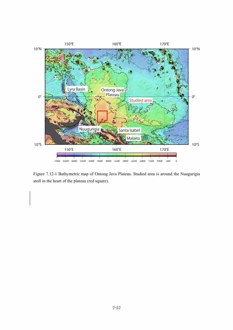
7-57

Figure 7.12-1 Bathymetric map of Ontong Java Plateau. Studied area is around the Nuugurigia atoll in the heart of the plateau (red square).

7-58

(2) Dredge system

The dredge system during MR12-03 is illustrated in Figures 7.12-2 and 7.12-3. Chief components of the system are a transponder, a lead wire, a chain, weights, a pipe dredge, fuse wires, life wires, and a chain-bag dredge (box-type or cylinder-type). The dredge assemblages were connected with a ship-board winch wire (17mm in diameter; 24.2 ton for breaking force). 1. The transponder is used to estimate the position and depth of the dredge system. It is

attached on the winch wire 50 m above its end. 2. The lead wire is 200 m long and 12 mm in diameter. The breaking force is 7.24 ton. It is

connected with the winch wire by shackles (3.15 ton) and a swivel (5 ton). 3. The chain is used to stabilize the dredge on the sea floor during operation. It is 5 m long and

19 mm in diameter. It is connected with the lead wire by shackles (3.25 ton) and a swivel (5 ton).

4. The weights keep the dredge on the sea floor during operation. A weight is 50 kg. Four weights are assembled and are connected with the chain by a fuse wire (0.25 m long and 8 mm in diameter; 3.22 ton for breaking force), a life wire covered with a hose (1.7 m long and 10 mm in diameter; 5.03 ton for breaking force), shackles (2 ton), and a swivel (1 ton).

5. The pipe dredge is connected with the chain by a fuse wire (0.25 m long and 8 mm in diameter; 3.22 ton for breaking force), a life wire covered with a hose (1.0 m long and 10 mm in diameter; 5.03 ton for breaking force), shackles (0.6 ton; 1.2 ton), and a swivel (1 ton).

6. A dredge is connected with the chain by a fuse wire (0.25 m long and 8 mm in diameter; 3.22 ton for breaking force), a life wire covered with a hose (5 m long and 10 mm in diameter; 5.03 ton for breaking force), shackles (0.6 ton; 2 ton; 3.25 ton), a swivel (3 ton), and a master ring (3.2 ton). Either box-type or cylinder-type dredges were used at each dredge site. The box-type dredge has a square jaw (60 × 45 cm) with a chain-bag and a box-type bucket. The cylinder-type dredge has a round jaw (65 cm in diameter) with tied chains behind it.

7-59

Figure 7.12-2 Dredge system with a box-type dredge.

7-60

Figure 7.12-3 Dredge system with a cylinder-type dredge.

7-61

(3) Results

Six dredges were conducted on the flanks of the three cones from August 6th to 8th, 2012. The dredge tracks were designed to haul the dredge on steep slopes from the bottom of the cones. The dredge tracks are shown in Figure 7.12-4. The position and depth of the dredge sites are summarized in Table 7.12-1. D1 (2012/8/6) The slope where the dredge was conducted is between two submarine ridges extending east and south on the largest cone. The dredge started at the bottom (1480 m deep) and ended halfway up of the cone. The box-type dredge was used. We had some strong bites during the dredge, although a few samples were recovered.

Recovered samples were pieces of Fe-Mn oxides and a lithic fragment. This fragment is a highly vesiculated and oxidized scoria. The maximum thickness of Fe‒Mn oxides is 5 mm. Some sands with small pieces of Fe‒Mn oxides were recovered in the pipe dredge.

D2 (2012/8/6) The dredge was conducted on the eastern slope north of the submarine ridge extending east on the largest cone. The dredge started at the bottom (1484 m deep) and ended halfway up of the cone. The box-type dredge was used. We had some strong bites during the dredge, although a few samples were recovered again.

Recovered samples were a pillow fragment and pieces of Fe-Mn oxides. The pillow fragment is an olivine-phyric basalt with moderate visicularity. Olivines are strongly altered. The recovered sample has ~10 mm thick altered glassy margin. Mn-coat is ~5 mm thick. Some sands were also recovered in the pipe dredge.

D3 (2012/8/7) The dredge was conducted on the southeastern slope of the north cone. The dredge started at the bottom (1481 m deep) and ended close to the top of the cone. The box-type dredge was used. We had some strong bites during the dredge, although a few samples were recovered, as always.

Recovered sample was Fe-Mn oxides. The maximum thickness of Fe‒Mn oxides is 20 mm. A lithic fragment is included in one of Fe-Mn oxides samples. This fragment is highly altered and vesiculated. It includes altered olivines. Vesicles are filled with secondary minerals.

7-62

D4 (2012/8/7) The dredge was conducted on the eastern slope of the west cone. The dredge started at the bottom (1505 m deep) and ended close to the top of the cone. The box-type dredge was used. We had some strong bites during the dredge. Finally, the dredge was stucked and the fuse wire was cut. However, samples were recovered successfully.

Recovered samples were a pumice, a volcaniclastic rock, and some pieces of Fe‒Mn oxides. The pumice is highly vesiculated and altered. It may be exotic because it has no Mn-coat. The volcaniclastic rock includes some basaltic fragment that is highly vesiculated and altered. It is covered by thick Mn-coat (35mm).

D5 (2012/8/8) The slope where the dredge was conducted is the same as D2 on the largest cone. The dredge started at the bottom (1478 m deep) and ended close to the top of the cone. The cylinder-type dredge was used on this day. We had some strong bites during the dredge, although a few samples were recovered, as always.

Recovered samples were a pillow fragment and a chunk of Fe‒Mn oxides. The pillow fragment is an olivine-phyric basalt. Olivines are strongly altered. It is strongly vesiculated and vesicles are aligned to form some concentrated layers. Some vesicles were filled with secondary minerals. Mn-coat is 13 mm thick. The chunk of Fe‒Mn oxides is 30 mm thick. It includes hyaloclastite on its edge. Some sands were also recovered in the pipe dredge.

D6 (2012/8/8) The dredge was conducted on the southern slope of the largest cone. The dredge started at the bottom (1503 m deep) and ended close to the top of the cone. The cylinder-type dredge was used. We had some strong bites during the dredge. Finally, the dredge was stucked and the fuse wire was cut. However, samples were recovered successfully.

Recovered samples were some large pieces of Fe‒Mn oxides and a pumice. The Fe‒Mn oxides had some lithic fragments (oxidized scoria) on one side. One rock was associated with carbonates. The maximum thickness of Fe‒Mn oxide fragments is 35 mm. The pumice is highly vesiculated and altered. It may be exotic because it has only very thin Mn-coat. Some sands with small pieces of Fe‒Mn oxides were also recovered in the pipe dredge.

(4) Interpretations Recovered samples show a wide variety of rock types, including pillow basalt, scoria,

7-63

pumice, and hyaloclastite. Pumices would be exotic as they have film (or nil) of Mn-coat. However, we suggest that scoria fragments are in-situ (either from the cones or the Nuugurigia volcano) because we recovered several samples including scoria covered by thick Fe‒Mn oxides at the same dredge site (D6). Some other scoria fragments with similar texture were also recovered at other dredge sites. The presence of scoria and hyaloclastite indicates subaerial or shallow-water submarine eruption. In contrast, the cones were also formed by submarine eruption, as suggested by the emplacement of pillow lavas. The thickness of Mn‒coat on these rocks varies, ranging from 5 to 35 mm. This fact may suggest multiple eruption history, although further post-cruise study is required to explore it.

Figure 7.12-4 Bathytmetric map of the studied cones. The dredge tracks are shown by red lines

annotated by dredge number.

7-64

Table 7.12-1 Summary table for six dredges in MR12-03.

Table 7.12-2 Event log for dredges and underway geophysical survey around Nuugurigia.

7-65

(5) Remarks for topography and structure of Nuugurigia; preliminary results of underway geophysical survey Geophysical survey was conducted during the transit into/out of the dredge sites and at night time between dredges with multi narrow beam echo sounding system, sub-bottom profiler, towing cesium magnetometer, ship-board three-component magnetometer, and gravity meter (c.f. Section 6.6). The chief objectives of underway geophysical survey are (1) to confirm the topography of the cones where we dredge, (2) to explore the submarine structure of the Nuugurigia volcano on which the cones sits, and (3) to find other cones where there are possible loci of peripheral eruptions of the volcano. The survey tracks were designed to traverse the northen and western flanks of Nuugurigia (Figure 7.12-5).

We passed over the dredge sites several times to obtain precise bathymetry, acoustic reflection, and sub-bottom profiling data for the cones. We confirmed that the cones have thin or nil sediment covers on their slopes. The largest cone has a conical shape with two ridges extending east and south. The north and west cones are different from the largest cone in terms of topography; they have a characteristic elongated shape. Orientations of the north and west cones together with the ridges on the largest cone seem to be random.

During the survey on the flanks of Nuugurigia, we found several cones that are similar to the cones, where we dredged, in terms of shape and size. They also have strong acoustic reflection, suggesting thin or nil sediments on the cones, like the cones we dredged. Although the surveyed area is limited, the cones are clustered near the dredge sites. We assume that the region around dredge sites is the place of repeated peripheral eruption on a northeast-trending submarine ridge of the Nuugurigia volcano. The cones we found in this cruise would be potential sites for future dredges and dives.

The data for gravity and geomagnetics will be processed and analyzed to explore the structure of the Nuugurigia volcano after the cruise.

7-66

Figure 7.12-5 Bathymetric map around Nuugurigia. Tracks for underway geophysical survey are

shown by colored lines: red; August 5th, green; August 6th, blue; August 7th, and pink; August 8th.

Thin gray thin lines are survey tracks by previous cruises.

7-67

References

1. Anderson, D. L., 2005. Large Igneous Provinces, delamination, and fertile mantle.

Elements 1, 271-275.

2. Anderson, D. L., Zhang, Y-S., Tanimoto, T., 1992. Plume heads, continental lithosphere,

flood basalts, and tomography. In: Storey, B. C., Alabaster, T., and Pankhurst, R. J. (eds)

Magmatism and Causes of Continental Break-up. Geol. Soc. London Spec. Pub. 68,

99-124.

3. Campbell, I. H., 2007. Testing the plume theory. Chem. Geol. 241, 153-176.

4. Erba, E., Bottini, C., Weissert, H. J., and Keller, C. E., 2010. Calcareous nannoplankton

response to surface-water acidification around oceanic anoxic event 1a. Science 329,

428-432.

5. Larson, R. L. and Erba, E., 1999. Onset of the mid-Cretaceous greenhouse in the

Barremian-Aptian: igneous events and the biological, sedimentary, and geochemical

responses. Paleocean. 14, 663-678.

6. Fitton, J. G. and Godard, M., 2004. Origin and evolution of magmas on the Ontong Java

Plateau. In: Fitton, J. G., Mahoney, J. J., Wallace, P. J. and Saunders, A. D. (eds) Origin

and Evolution of the Ontong Java Plateau. Geological Society (London) Special

Publication 229, 151-178.

7. Ingle, S., Coffin, M. F., 2004. Impact origin for the greater Ontong Java Plateau? Earth

Planet. Sci. Lett. 218, 123-134.

8. Jones, A. P., Price, G. D., Price, N. J., De Carli, P. S., Clegg, R. A., 2002. Impact

induced melting and the development of large igneous provinces. Earth Planet. Sci. Lett

202, 551-561.

9. Kerr, A. C. and Mahoney, J. J., 2007. Oceanic plateaus: Problematic plumes, potential

paradigms. Chem. Geol. 241, 332-353.

7-68

10. Korenaga, J., 2004. Mantle mixing and continental breakup magmatism. Earth Planet.

Sci. Lett. 218, 463-473.

11. Korenaga, J., 2005. Why did not the Ontong Java Plateau form subaerially? Earth

Planet. Sci. Lett. 234, 385-399.

12. Lustrino, M., 2005. How the delamination and detachment of lower crust can influence

basaltic magmatism. Earth-Sci. Rev. 72, 21-38.

13. Mahoney, J. J., Storey, M., Duncan, R. A., Spencer, K. J., Pringle, M., 1993.

Geochemistry and geochronology of the Ontong Java Plateau. In: Pringle, M., Sager, W.,

Sliter, W., and Stein, S. (eds) The Mesozoic Pacific. Geology, Tectonics, and Volcanism.

AGU Geophys. Monogr. 77, 233-261.

14. Richards, M. A., Duncan, R. A., and Courtillot, V., 1989. Flood basalts and hotspot

tracks: plume heads and tails. Science 246, 103-107.

15. Rogers, G. C., 1982. Oceanic plateaus as meteorite impact signatures. Nature 299,

341-342.

16. Tarduno, J. A., Brinkman, D. B., Renne, P. R., Cottrell, R. D., Scher, H. and Castillo, P.,

1998. Evidence for extreme climatic warmth from Late Cretaceous Arctic vertebrates.

Science 282, 2241-2244.

17. Tejada, M. L. G., J. J. Mahoney, C. R. Neal, R. A. Duncan, and M. G. Petterson, 2002.

Basement geochemistry and geochronology of Central Malaita, Solomon Islands, with

implications for the origin and evolution of the Ontong Java Plateau. J. Petrol. 43,

449-484.

18. Tejada, M. L. G., J. J. Mahoney, P. R. Castillo, S. P. Ingle, H. C. Sheth, and D. Weis,

2004. Pin-pricking the elephant: Evidence on the origin of the Ontong Java Plateau

from Pb-Sr-Hf-Nd isotopic characteristics of ODP Leg 192 basalts. In: Fitton, J. G. et al.

(eds) Origin and Evolution of the Ontong Java Plateau. Geol. Soc.(London) Spe. Pub.

229, 133-150.

7-69

19. Tejada, M. L. G., Suzuki, K., Kuroda, J., Coccioni, R., Mahoney, J. J., Ohkouchi, N.,

Sakamoto, T., and Tatsumi, Y., 2009. Ontong Java Plateau eruption as a trigger for the

Early Aptian oceanic event. Geology 37, 855-858.

r/v mirai cruise report mr12-03 · 2014-09-29 · at first, engine trouble during this cruise...

Documents