Rotation Averaging and Strong Duality

Anders Eriksson1, Carl Olsson2,3, Fredrik Kahl2,3 and Tat-Jun Chin4

1School of Electrical Engineering and Computer Science, Queensland University of Technology2Department of Electrical Engineering, Chalmers University of Technology

3Centre for Mathematical Sciences, Lund University4School of Computer Science, The University of Adelaide

Abstract

In this paper we explore the role of duality principleswithin the problem of rotation averaging, a fundamentaltask in a wide range of computer vision applications. Inits conventional form, rotation averaging is stated as a min-imization over multiple rotation constraints. As these con-straints are non-convex, this problem is generally consid-ered challenging to solve globally. We show how to circum-vent this difficulty through the use of Lagrangian duality.While such an approach is well-known it is normally notguaranteed to provide a tight relaxation. Based on spectralgraph theory, we analytically prove that in many cases thereis no duality gap unless the noise levels are severe. This al-lows us to obtain certifiably global solutions to a class ofimportant non-convex problems in polynomial time.

We also propose an efficient, scalable algorithm that out-performs general purpose numerical solvers and is able tohandle the large problem instances commonly occurring instructure from motion settings. The potential of this pro-posed method is demonstrated on a number of differentproblems, consisting of both synthetic and real-world data.

1. Introduction

Rotation averaging appears as a subproblem in manyimportant applications in computer vision, robotics, sen-sor networks and related areas. Given a number of rela-tive rotation estimates between pairs of poses, the goal is tocompute absolute camera orientations with respect to somecommon coordinate system. In computer vision, for in-stance, non-sequential structure from motion systems suchas [21, 11, 22] rely on rotation averaging to initialize bundleadjustment. The overall idea is to consider as much data aspossible in each step to avoid suboptimal reconstructions.In the context of rotation averaging this amounts to using asmany camera pairs as possible.

The problem can be thought of as inference on the cam-

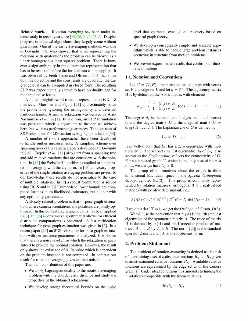
Figure 1: In many structure from motion pipelines, cam-era orientations are estimated with rotation averaging fol-lowed by recovery of camera centres (red) and 3D structure(blue). Here are three solutions corresponding to differentlocal minima of the same rotation averaging problem.

era graph. An edge (i, j) in this undirected graph representsa relative rotation measurement Rij and the objective is tofind the absolute orientation Ri for each vertex i such thatRiRij = Rj holds (approximately in the presence of noise)for all edges. The problem is generally considered difficultdue to the need to enforce non-convex rotation constraints.Indeed, both L1 and L2 formulations of rotation averagingcan have local minima, see Fig. 1. Wilson et al. [28] studiedlocal convexity of the problem and showed that instanceswith large loosely connected graphs are hard to solve withlocal, iterative optimization methods.

In contrast, our focus is on global optimality. In thispaper we show that convex relaxation methods can in factovercome the difficulties with local minima in rotation aver-aging. We utilize Lagrangian duality to handle the quadraticnon-convex rotation constraints. While such an approach isnormally not guaranteed to provide a tight relaxation wegive analytical error bounds that guarantee there will be noduality gap. For instance, it is sufficient that each angularresidual is less than 42.9◦ to ensure optimality for completecamera graphs. Additionally, we develop a scalable and ef-ficient algorithm, based on block coordinate descent, thatoutperforms standard semidefinite program (SDP) solversfor this problem.

1

arX

iv:1

705.

0136

2v2

[cs

.CV

] 2

9 N

ov 2

017

Related work. Rotation averaging has been under in-tense study in recent years, see [19, 20, 21, 2, 25, 8]. Despiteprogress in practical algorithms, they largely come withoutguarantees. One of the earliest averaging methods was dueto Govindu [15], who showed that when representing therotations with quaternions the problem can be viewed as alinear homogeneous least squares problem. There is how-ever a sign ambiguity in the quaternion representation thathas to be resolved before the formulation can be applied. Itwas observed by Fredriksson and Olsson in [14] that sinceboth the objective and the constraints are quadratic, the La-grange dual can be computed in closed form. The resultingSDP was experimentally shown to have no duality gap formoderate noise levels.

A more straightforward rotation representation is 3 × 3matrices. Martinec and Pajdla [21] approximately solvethe problem by ignoring the orthogonality and determi-nant constraints. A similar relaxation was derived by Arie-Nachimson et al. in [1]. In addition, an SDP formulationwas presented which is equivalent to the one we addresshere, but with no performance guarantees. The tightness ofSDP relaxations for 2D rotation averaging is studied in [30].

A number of robust approaches have been developedto handle outlier measurements. A sampling scheme overspanning trees of the camera graph is developed by Govinduin [16]. Enqvist et al. [11] also start from a spanning treeand add relative rotations that are consistent with the solu-tion. In [17] the Weiszfeld algorithm is applied to single ro-tation averaging with the L1 norm. In [18] convexity prop-erties of the single rotation averaging problem are given. Toour knowledge these results do not generalize to the caseof multiple rotations. In [9] a robust formulation is solvedusing IRLS and in [3] Cramer-Rao lower bounds are com-puted for maximum likelihood estimators, but neither withany optimality guarantees.

A closely related problem is that of pose graph estima-tion, where camera orientations and positions are jointly op-timized. In this context Lagrangian duality has been applied[6, 7]. In [26] a consensus algorithm that allows for efficientdistributed computations is presented. A fast verificationtechnique for pose graph estimation was given in [5]. In arecent paper [23] an SDP relaxation for pose graph estima-tion with performance guarantees is analyzed. It is shownthat there is a noise level β for which the relaxation is guar-anteed to provide the optimal solution. However, the resultonly shows the existence of β. Its value which is dependenton the problem instance is not computed. In contrast ourresult for rotation averaging gives explicit noise bounds.

The main contributions of this paper are:• We apply Lagrangian duality to the rotation averaging

problem with the chordal error distance and study theproperties of the obtained relaxations.

• We develop strong theoretical bounds on the noise

level that guarantee exact global recovery based onspectral graph theory.

• We develop a conceptually simple and scalable algo-rithm which is able to handle large problem instancesoccurring in structure from motion problems.

• We present experimental results that confirm our theo-retical findings.

1.1. Notation and Conventions

Let G = (V,E) denote an undirected graph with vertexset V and edge setE and let n = |V |. The adjacency matrixA is by definition the n× n matrix with elements

aij =

{0 (i, j) /∈ E1 (i, j) ∈ E for i, j = 1, . . . , n. (1)

The degree di is the number of edges that touch vertexi, and the degree matrix D is the diagonal matrix D =diag (d1, . . . , dn). The Laplacian LG of G is defined by

LG = D −A. (2)

It is well-known that LG has a zero eigenvalue with mul-tiplicity 1. The second smallest eigenvalue λ2 of LG, alsoknown as the Fiedler value, reflects the connectivity of G.For a connected graph G, which is the only case of interestto us, we always have λ2 > 0.

The group of all rotations about the origin in threedimensional Euclidean space is the Special OrthogonalGroup, denoted SO(3). This group is commonly repre-sented by rotation matrices, orthogonal 3 × 3 real-valuedmatrices with positive determinant, i.e.,

SO(3) ∈ {R ∈ R3×3 | RTR = I, det(R) = 1}. (3)

If we omit det(R)=1, we get the Orthogonal Group, O(3).We will use the convention that λi(A) is the i:th smallest

eigenvalue of the symmetric matrix A. The trace of matrixA is denoted by tr (A) and the Kronecker product of ma-trices A and B by A ⊗ B. The norm ‖A‖ is the standardoperator 2-norm and ‖A‖F the Frobenius norm.

2. Problem Statement

The problem of rotation averaging is defined as the taskof determining a set of n absolute rotationsR1, ..., Rn givendistinct estimated relative rotations Rij . Available relativerotations are represented by the edge set E of the cameragraph V . Under ideal conditions this amounts to finding then rotations compatible with the linear relations,

RiRij = Rj , (4)

for all (i, j) ∈ E. However, in the presence of noise, a solu-tion to (4) is not guaranteed to exist. Instead, it is typicallysolved in a least-metric sense,

minR1,...,Rn

∑(i,j)∈E

d(RiRij , Rj)p, (5)

where p ≥ 1 and d(·, ·) is a distance function.A number of distinct choices of metrics on SO(3) exist,

see Hartley et al. [19] for a comprehensive discussion. Inthis work we restrict ourselves to the chordal distance, themost commonly used metric when analyzing Lagrangianduality in rotation averaging. It has proven to be a conve-nient choice as it is quadratic in its entries leading to a par-ticularly simple derivation and form of the associated dualproblem.

The chordal distance between two rotations R and S isdefined as their Euclidean distance in the embedding space,

d(R,S) = ‖R− S‖F . (6)

It can be shown [19] that the chordal distance can also bewritten as d(R,S) = 2

√2 sin |α|2 , where α is the rotation

angle of RS−1. With the this choice of metric, the rotationaveraging problem is defined as

arg minR1,...,Rn∈SO(3)

∑(i,j)∈E

‖RiRij −Rj‖2F , (7)

which, with trace notation, can be simplified to

arg minR1,...,Rn∈SO(3)

−∑

(i,j)∈E

tr(RiRijR

Tj

), (8)

which constitutes our primal problem.It will be convenient with a compact matrix formulation.

Let

R =

0 a12R12 ... a1nR1n

a21R21 0 ... a2nR2n

.... . .

...an1Rn1 an2Rn2 ... 0

, (9)

where Rij = RTji and aij are the elements of the adjacencymatrix A of the camera graph G and let

R =[R1 R2 . . . Rn

]. (10)

We may now write the primal problem as

(P ) min −tr(RRRT

)s.t. R ∈ SO(3)n.

(11)

3. Optimality Conditions3.1. Necessary Local Optimality Conditions

We now turn to the KKT conditions of our primal prob-lem (P ). The constraint set R ∈ SO(3)n consists of two

types of constraints; the orthogonality constraints RTi Ri =I and the determinant constraints det(Ri) = 1.

Consider relaxing the rotation averaging problem by re-moving the determinant constraint,

(P ′) min −tr(RRRT

)s.t. R ∈ O(3)n.

(12)

The constraint R ∈ O(3)n still requires the Ri’s to be or-thogonal. The orthogonal matrices consist of two disjoint,non-connected sets, with determinants 1 and −1 respec-tively. Hence, any local minimizer to the problem (P ) alsohas to be a local minimizer, and therefore a KKT point, to(P ′). We note that orthogonality can be enforced by re-stricting the 3× 3 diagonal blocks of the symmetric matrixRTR to be identity matrices. If

Λ =

Λ1 0 0 . . .0 Λ2 0 . . .0 0 Λ3 . . ....

......

. . .

(13)

is a symmetric matrix then the Lagrangian can be written

L(R,Λ) = −tr(RRRT

)− tr

(Λ(I −RTR)

)= −tr

(R(Λ− R)RT

)− tr (Λ) .

(14)

Taking derivatives gives the KKT equations

(Stationarity)

(Λ∗ − R)R∗T

= 0 (15a)(Primal feasibility)

R∗ ∈ SO(3)n. (15b)

Equation (15a) states that the rows of a local minimizer R∗

will be eigenvectors of the matrix Λ∗ − R with eigenvaluezero. This allows us to compute the optimal Lagrange mul-tiplier Λ∗ from a given minimizer R∗. By (15a) we see that

Λ∗iR∗Ti =

∑j 6=i

aijRijR∗Tj ⇐⇒ Λ∗i =

∑j 6=i

aijRijR∗Tj R∗i

(16)for i = 1, . . . , n.

Lemma 3.1. For a stationary point R∗ to the primal prob-lem (P ), we can compute the corresponding Lagrangianmultiplier Λ∗ in closed form via (16).

3.2. Sufficient Global Optimality Conditions

We begin this section by deriving the Lagrange dual of(P ) which is a semidefinite program that we will use foroptimization in later sections. The dual problem is definedby

maxΛ−R�0

minR

L(R,Λ). (17)

Since the (unrestricted) optimum of minR L(R,Λ) is either−tr (Λ), when Λ− R � 0, or −∞ otherwise, we get

(D) maxΛ−R�0

−tr (Λ) . (18)

It is clear (through standard duality arguments) that (D)gives a lower bound on (P ). Furthermore, if R∗ is a sta-tionary point with corresponding Lagrangian multiplier Λ∗

that satisfies Λ∗ − R � 0 then Λ∗ is feasible in (D) and by(16), −tr (Λ∗) = −tr

(R∗RR∗T

), which shows that there

is no duality gap between (P ) and (D). Thus, the convexprogram (D) provides a way of solving the non-convex (P )when Λ∗ − R � 0.

It also follows that for the stationary point R∗ we havetr(R∗Λ∗R∗T

)= tr

(R∗RR∗T

)due to (15a). We further

note that if Λ∗ − R � 0 then by definition it is true that

xT(

Λ∗ − R)x ≥ 0, (19)

for any 3n-vector x. In particular, for any R ∈ O(3)n,

0 ≤ tr(R(Λ∗ − R)RT

)= tr (Λ∗)− tr

(RRRT

)= tr

(R∗Λ∗R∗T

)− tr

(RRRT

),

(20)which shows that −tr

(R∗RR∗T

)≤ −tr

(RRRT

)for all

R ∈ O(3)n, that is, R∗ is the global optimum.

Lemma 3.2. If a stationary point R∗ with correspondingLagrangian multiplier Λ∗ fulfills Λ∗ − R � 0 then:

1. There is no duality gap between (P ) and (D).

2. R∗ is a global minimum for (P ).

In the remainder of this paper we will study under whichconditions Λ∗ − R � 0 holds and derive an efficient imple-mentation for solving (D).

4. Main ResultIn this section, we will state our main result which gives

error bounds that guarentee that that strong duality holdsfor our primal and dual problems. From a practical point ofview, the result means that it is possible to solve a convexsemidefinite program and obtain the globally optimal solu-tion to our non-convex problem, which is quite remarkable.

4.1. Strong Duality Theorem

Returning to our initial, primal rotation averaging prob-lem (7). The goal is to find rotations Ri and Rj such thatthe sum of the residuals ‖RiRij −Rj‖2F is minimized. Forstrong duality to hold, we need to bound the residual error.

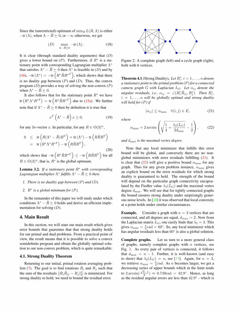
Figure 2: A complete graph (left) and a cycle graph (right),both with 6 vertices.

Theorem 4.1 (Strong Duality). LetR∗i , i = 1, . . . , n denotea stationary point to the primal problem (P ) for a connectedcamera graph G with Laplacian LG. Let αij denote theangular residuals, i.e., αij = ∠(R∗i Rij , R

∗j ). Then R∗i ,

i = 1, . . . , n will be globally optimal and strong dualitywill hold for (P ) if

|αij | ≤ αmax ∀(i, j) ∈ E, (21)

where

αmax = 2 arcsin

√1

4+λ2(LG)

2dmax− 1

2

, (22)

and dmax is the maximal vertex degree.

Note that any local minimizer that fulfills this errorbound will be global, and conversely there are no non-global minimizers with error residuals fulfilling (21). Itis clear that (22) will give a positive bound αmax for anygraph. Thus for any given problem instance, αmax givesan explicit bound on the error residuals for which strongduality is guaranteed to hold. The strength of the boundwill depend on the particular graph connectivity encapsu-lated by the Fiedler value λ2(LG) and the maximal vertexdegree dmax. We will see that for tightly connected graphsthe bound ensures strong duality under surprisingly gener-ous noise levels. In [28] it was observed that local convexityat a point holds under similar circumstances.

Example. Consider a graph with n = 3 vertices that areconnected, and all degrees are equal, dmax = 2. Now fromthe Laplacian matrix LG, one easily finds that λ2 = 3. Thisgives αmax = π

3 rad = 60◦. So, any local minimizer whichhas angular residuals less than 60◦ is also a global solution.

Complete graphs. Let us turn to a more general classof graphs, namely complete graphs with n vertices, seeFig. 2. As every pair of vertices is connected, it followsthat dmax = n − 1. Further, it is well-known (and easyto show) that λ2(LG) = n, see [13]. Again, for n = 3,we retrieve αmax = π

3 rad. As n becomes larger, we get adecreasing series of upper bounds which in the limit tendsto 2 arcsin(

√3−12 ) ≈ 0.749rad = 42.9◦. Hence, as long

as the residual angular errors are less than 42.9◦ - which is

quite generous from a practical point of view - we can com-pute the optimal solution via a convex program. Also notethat this bound holds independently of n.

Corollary 4.1. For a complete graph G with n vertices,the residual upper bound αmax = 2 arcsin(

√3−12 ) ≈

0.749rad = 42.9◦ ensures global optimality and strong du-ality for any n.

Cycle graphs. Now consider the other spectrum interms of graph connectivity, namely cycle graphs. A cy-cle graph has a single cycle, or in other words, everyvertex in the camera graph has degree two (dmax = 2)and the vertices form a closed chain (Fig. 2). From theliterature, we have that the Fiedler value λ2 = 2(1 −cos 2π

n ). Inserting into (22) and simplifying, we get αmax =

2 arcsin(√

14 + sin2(πn )− 1

2

). Again, for n = 3, we re-

trieve αmax = π3 rad. For larger values of n, the upper

bound decreases rapidly. In fact, the upper bound is quiteconservative and it is possible to show a much stronger up-per bound using a different analysis. In the appendix, weprove the following theorem.

Theorem 4.2. Let R∗i , i = 1, . . . , n denote a stationarypoint to the primal problem (P ) for a cycle graph with nvertices. Let αij denote the angular residuals, i.e., αij =

∠(R∗i Rij , R∗j ). Then, R∗i , i = 1, . . . , n will be globally

optimal and strong duality will hold for (P ) if |αij | ≤ πn for

all (i, j) ∈ E.

Requiring that the angular residuals |αij | must be lessthan π/n for the global solution may seem like a restriction,but it is actually not. To see this, note that a non-optimalsolution to the rotation averaging problem can be obtainedby choosing R1 such that the first residual α12 is zero, andthen continuing in the same fashion such that all but the lastresidual α1n in the cycle is zero. In the worst case, α1n = π.However, this is (obviously) non-optimal. A better solutionis obtained if we distribute the angular residual error evenlyso that αij = α = α1n

n (which is always possible, see The-orem 23 in [10]). In conclusion, the angular residuals |αij |of the globally optimal solution for a cycle graph is alwaysless than or equal to π

n , and conversely, if the angular resid-ual is larger than π

n for a local minimizer, then it does notcorrespond to the global solution.

In Fig. 1, we have a real example of an orbital cameramotion which is close to a cycle. It may seem hard to de-termine if the camera motion consists of one or more loopsaround the object - we give three different local minima forthis example. Still, applying formula (22) for this instancegives αmax = 8.89◦ which is typically sufficient in prac-tice to ensure that the optimal solution can be obtained bysolving a convex program. Before developing an actual al-gorithm, we shall prove our main result on strong duality.

4.2. Proof of Theorem 4.1

Recall that a sufficient condition for strong duality tohold is that Λ∗ − R � 0 (Lemma 3.2). To prove Theo-rem 4.1 we will show that this is true under the conditionsof the theorem.

To simplify the presentation we denote the residual rota-tions Eij = R∗i RijR

∗Tj and define

DR∗ =

R∗1 0 0 . . .0 R∗2 0 . . .0 0 R∗3 . . ....

......

. . .

. (23)

Then DR∗(Λ∗ − R)DTR∗ =

∑j 6=1 a1jE1j −a12E12 −a13E13 . . .

−a12ET12

∑j 6=2 a2jE2j −a23E23 . . .

−a13ET13 −a23ET23

∑j 6=3 a3jE3j . . .

......

.... . .

.(24)

Note that∑j 6=i aijEij = 1

2

∑j 6=i aij(Eij+ETij) by symme-

try of Λ∗. Since DR∗ is orthogonal, the matrix Λ∗ − R ispositive semidefinite if and only if DR∗(Λ∗ − R)DT

R∗ is.In the noise free case we note that the residual rotations

will fulfill Eij = I and therefore

DR∗(Λ∗ − R)DTR∗ = LG ⊗ I3. (25)

In the general noise case our strategy will therefore be tobound the eigenvalues of DR∗(Λ∗ − R)DT

R∗ by those ofLG for which well-known estimates exist. Thus, we willanalyze the difference and define the matrix

∆ = DR∗(Λ∗ − R)DTR∗ − LG ⊗ I3. (26)

The following results characterize the eigenvalues of ∆.

Lemma 4.1. Let ∆ij , i = 1, ..., n, j = 1, ..., n be the 3× 3sub-blocks of ∆. If λ is an eigenvalue of ∆ then

|λ| ≤n∑j=1

‖∆ij‖ for some i = 1, . . . , n. (27)

Proof. The proof is similar to that of Gerschgorin’s theorem[12]. Let ∆x = λx, with ‖x‖ = 1. Then λxi =

∑j ∆ijxj .

Now pick i such that ‖xi‖ ≥ ‖xj‖ for all j. Then

|λ| =∥∥∥∥λ xi‖xi‖

∥∥∥∥ =

∥∥∥∥∥∥n∑j=1

∆ijxj‖xi‖

∥∥∥∥∥∥ ≤n∑j=1

‖∆ij‖. (28)

Lemma 4.2. Denote αmax the largest (absolute) residualangle of all Eij and assume 0 ≤ αmax ≤ π

2 . Then

‖∆ii‖ ≤ 2di sin2(αmax

2) ∀i = 1, . . . n, (29)

where di is the degree of vertex i.

Proof. It is easy to see that by applying a change of coordi-nates Eij can be written

Eij = Vij

cos(αij) − sin(αij) 0sin(αij) cos(αij) 0

0 0 1

V Tij , (30)

and therefore

1

2(Eij + ETij) = Vij

cos(αij) 0 00 cos(αij) 00 0 1

V Tij . (31)

This gives

(cos(αij)− 1)I � 1

2(Eij + ETij)− I � 0, (32)

and since ∆ii =∑j 6=i aij

(12 (Eij + ETij)− I

)we get

di(cos(αmax)− 1)I � ∆ii � 0. (33)

Thus ‖∆ii‖ ≤ di(1− cos(αmax)) = 2di sin2(αmax

2 ).

Lemma 4.3. If 0 ≤ αmax ≤ π2 and i 6= j then

‖∆ij‖ ≤ 2aij sin(αmax

2). (34)

Proof. To estimate the off-diagonal blocks ‖∆ij‖ =aij‖I − Eij‖ we note that for a unit vector v we have√‖v − Eijv‖2 =

√‖v‖2 − 2 cos∠(v, Eijv) + ‖Eijv‖2

≤√

2(1− cos(αij)), (35)

where ∠(v, Eijv) is the angle between v and Eijv. Further-more, we will have equality if v is perpendicular to the ro-tation axis of Eij . Therefore

‖∆ij‖ = aij

√2(1− cos(αij)) ≤ 2aij sin(

αmax

2). (36)

Summarizing the results in Lemmas 4.1- 4.3 we get thatthe eigenvalues λ of ∆ fulfill

|λ(∆)| ≤ 2di sin2(αmax

2) +

∑j 6=i

2aij sin(αmax

2)

≤ 2dmax sin(αmax

2)(

1 + sin(αmax

2)),

(37)

where dmax is the maximal vertex degree. Note that thesame bound holds for all eigenvalues of ∆, in particular, theone with the largest magnitude λmax(∆).

Now returning to our goal of showing that DR∗(Λ∗ −R)DT

R∗ � 0. Let N =[I I . . .

]T. The columns of N

will be in the nullspace of DR∗(Λ∗ − R)DTR∗ . Therefore

DR∗(Λ∗ − R)DTR∗ is positive semidefinite if DR∗(Λ∗ −

R)DTR∗ + µNNT is, and hence it is enough to show that

λ1

(DR∗(Λ∗ − R)DT

R∗ + µNNT)≥ 0 (38)

for sufficiently large µ. The Laplacian LG is positivesemidefinite with smallest eigenvalue λ1 = 0 and corre-sponding eigenvector v =

(1 1 . . . 1

)T. Furthermore,

as N = v ⊗ I3, it is clear that for sufficiently large µ wehave λ1(LG⊗I3 +µNNT ) = λ1(LG+µvvT ) = λ2(LG).Since

DR∗(Λ∗ − R)DTR∗ + µNNT = LG ⊗ I3 + µNNT + ∆,

(39)we therefore get

λ1(DR∗(Λ∗ − R)DTR∗ + µNNT ) ≥ λ2(LG)− |λmax(∆)|.

(40)

If the right-hand side is positive, then so is the left-handside. Using (37) for λmax(∆) yields the following result.

Lemma 4.4. The matrix Λ∗ − R is positive semidefinite if

λ2(LG)− 2dmax sin(αmax

2)(

1 + sin(αmax

2))≥ 0. (41)

By completing squares, one obtains the equivalent con-dition (

sin(αmax

2) +

1

2

)2

≤ λ2(LG)

2dmax+

1

4, (42)

which shows Theorem 4.1.

5. Solving the Rotation Averaging ProblemThe dual problem (D) is a convex semidefinite program,

and although it is theoretically sound and provably solvablein polynomial time by interior point methods [4], in practicesuch problems quickly become intractable as the dimensionof the entering variables grow.

In this section we present a first-order method for solvingsemidefinite programs with constant block diagonals. Ourapproach solves the dual of (D) and consists of two sim-ple matrix operations only, matrix multiplication and squareroots of 3 × 3 symmetric matrices, the latter which can besolved in closed form. Consequently, these two operationspermit a simple and efficient implementation without theneed for dedicated numerical libraries.

The dual of (D) is given by

minY�0

maxΛ−tr (Λ) + tr

(Y (Λ− R)

). (43)

Let the matrix Y be partitioned as follows,

Y =

Y11 Y12 ... Y1n

Y T12 Y22 ... Y2n

......

. . ....

Y T1n ... ... Ynn

(44)

where each block Yij ∈ R3×3 for i, j = 1, . . . , n. Since Λis block-diagonal (13) it is clear that the inner maximizationis unbounded when Yii− I3×3 6= 0 and zero otherwise. Wetherefore get

(DD) minY

−tr(RY)

s.t. Yii = I3, i = 1, ..., n,Y � 0.

(45)

Since Y � 0 it is clear that

−tr (Λ) + tr (Y (Λ−R∗)) ≥ −tr (Λ) ,

for all Λ of the form (13). Therefore (DD) ≥ (D) andassuming strong duality holds (D) = (P ). Furthermoreif R∗ is the global optimum of (P ) then Y = R∗TR∗ isfeasible in (45) which shows that (DD) = (P ).

Thus, when strong duality holds, recovering a primal so-lution to (P ) is then achieved by simply reading off the firstthree rows of Y ∗ and choosing their signs to ensure positivedeterminants of the resulting rotation matrices, see supple-mentary material for further details.

5.1. Block Coordinate Descent

In this section we present a block coordinate descentmethod for solving semidefinite programs with block diag-onal constraints on the form (45). This method is a general-ization of the row-by-row algorithms derived in [27].

Consider the following semidefinite program,

minS∈R3n×3

tr(WTS

)s.t.

[I ST

S B

]� 0.

(46)

This is a subproblem that arises when attempting to solve(DD) in (45) using a block coordinate descent approach,i.e., by fixing all but one row and column of blocks in (44)and reordering as necessary. It turns out that this subprob-lem has a particularly simple, closed form solution, estab-lished by the following lemma.

Lemma 5.1. Let B be a positive semidefinite matrix. Then,the solution to (46) is given by,

S∗ = −BW[(WTBW

) 12

]†. (47)

Here † denotes the Moore–Penrose pseudoinverse.

Proof. See supplementary material.

Algorithm 1 A block coordinate descent algorithm for thesemidefinite relaxation (DD) in (45).

input: R, Y (0) � 0, t = 0.repeat

· Select an integer k ∈ [1, . . . , n],·Bk: the result of eliminating the kth row and columnfrom Y t.·Wk: the result of eliminating the kth column and allbut the kth row from R.· S∗k = −BkWk

[(WTk BkWk

) 12]†

as in (47).

· Y t =[I S∗T

k

S∗k Bk

], (succeeded by the appropriate

reordering).· t = t+ 1

until convergence

6. Experimental ResultsIn this section we present an experimental study aimed

at characterizing the performance and computational effi-ciency of the proposed algorithm compared to existing stan-dard numerical solvers.

Synthetic data. In our first set of experiments wecompared the computational efficiency of the Levenberg-Marquardt (LM) algorithm [29], a standard nonlinear opti-mization method, Algorithm 1 and that of SeDuMi [24], apublicly available software package for conic optimization.

We constructed a large number of synthetic problem in-stances of increasing size, perturbed by varying levels ofnoise. Each absolute rotation was obtained by rotationabout the z-axis by 2π/n rad and by construction, forming acycle graph. The relative rotations were perturbed by noisein the form of a random rotation about an axis sampled froma uniform distribution on the unit sphere with angles nor-mally distributed with mean 0 and variance σ. The absoluterotations were initialized (if required) in a similar fashionbut with the angles uniformly distributed over [0, 2π] rad.

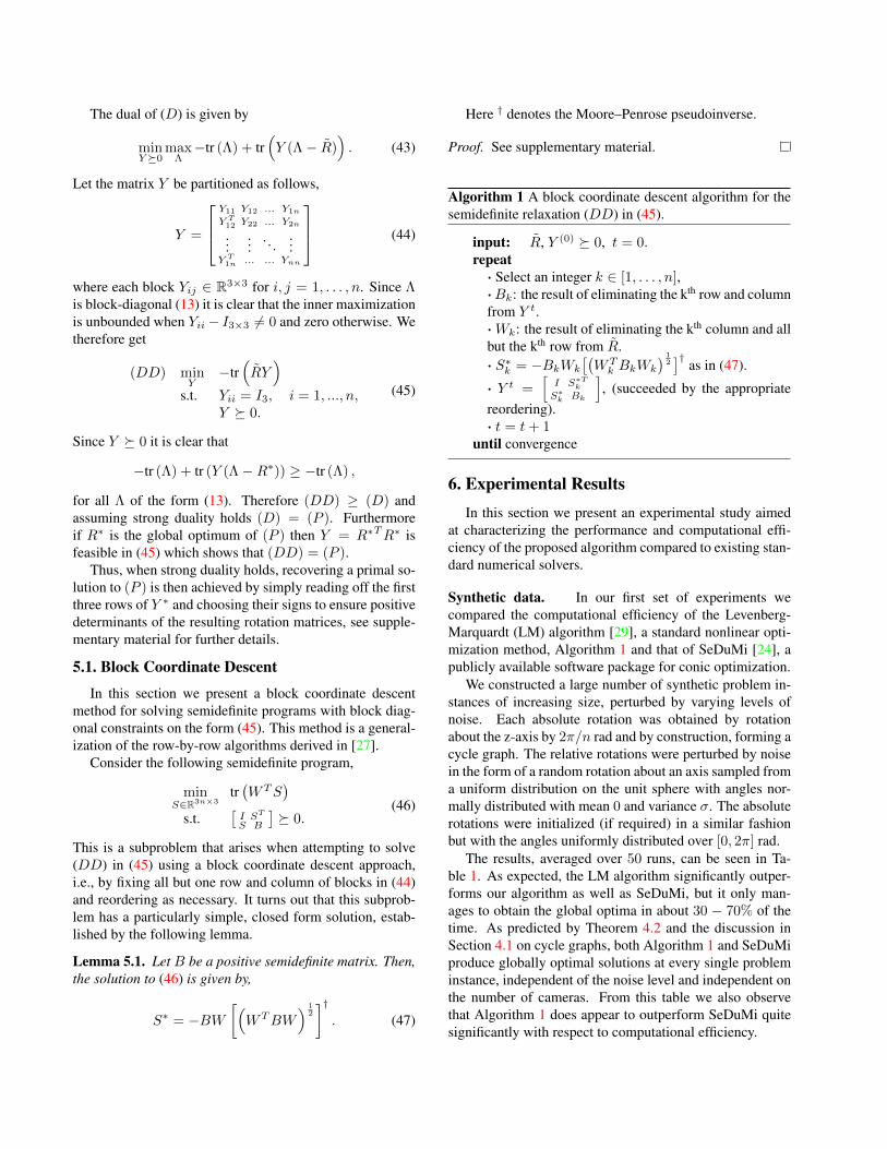
The results, averaged over 50 runs, can be seen in Ta-ble 1. As expected, the LM algorithm significantly outper-forms our algorithm as well as SeDuMi, but it only man-ages to obtain the global optima in about 30 − 70% of thetime. As predicted by Theorem 4.2 and the discussion inSection 4.1 on cycle graphs, both Algorithm 1 and SeDuMiproduce globally optimal solutions at every single probleminstance, independent of the noise level and independent onthe number of cameras. From this table we also observethat Algorithm 1 does appear to outperform SeDuMi quitesignificantly with respect to computational efficiency.

LM [29] Alg. 1 SeDuMi [24]

n σ [rad] avg.error (%) time[s] avg.error time[s] avg.error time[s]

20 0.2 1.49 (0.48) 0.012 9.34e-10 0.028 4.30e-09 0.5010.5 0.56 (0.73) 0.008 3.94e-08 0.023 3.72e-09 0.553

50 0.2 0.55 (0.50) 0.026 1.3e-09 0.17 6.85e-09 5.910.5 0.17 (0.58) 0.017 1.83e-07 0.33 2.00e-09 6.32

100 0.2 0.15 (0.55) 0.042 1.46e-07 8.89 5.31e-09 47.00.5 0.15 (0.45) 0.039 6.64e-08 7.97 7.41e-10 49.51

200 0.2 0.099 (0.40) 0.082 4.02e-08 17.01 4.15e-10 419.040.5 0.031 (0.33) 0.071 6.79e-08 29.4 6.91e-10 391.23

Table 1: Comparison of running times and resulting errors on synthetic data. Here the errors are given with respect to thelowest feasible objective function value found. The fraction of the times the global optima was reached by the LM algorithmis indicated along side the average error.

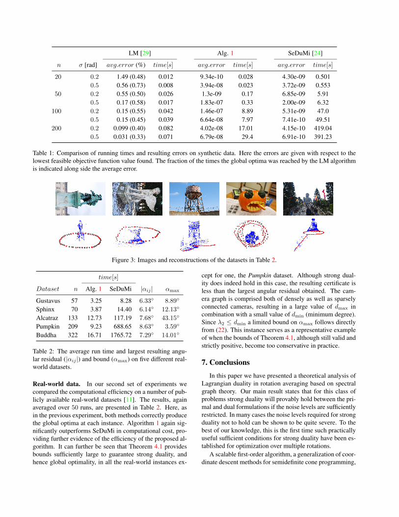
Figure 3: Images and reconstructions of the datasets in Table 2.

time[s]

Dataset n Alg. 1 SeDuMi |αij | αmax

Gustavus 57 3.25 8.28 6.33◦ 8.89◦

Sphinx 70 3.87 14.40 6.14◦ 12.13◦

Alcatraz 133 12.73 117.19 7.68◦ 43.15◦

Pumpkin 209 9.23 688.65 8.63◦ 3.59◦

Buddha 322 16.71 1765.72 7.29◦ 14.01◦

Table 2: The average run time and largest resulting angu-lar residual (|αij |) and bound (αmax) on five different real-world datasets.

Real-world data. In our second set of experiments wecompared the computational efficiency on a number of pub-licly available real-world datasets [11]. The results, againaveraged over 50 runs, are presented in Table 2. Here, asin the previous experiment, both methods correctly producethe global optima at each instance. Algorithm 1 again sig-nificantly outperforms SeDuMi in computational cost, pro-viding further evidence of the efficiency of the proposed al-gorithm. It can further be seen that Theorem 4.1 providesbounds sufficiently large to guarantee strong duality, andhence global optimality, in all the real-world instances ex-

cept for one, the Pumpkin dataset. Although strong dual-ity does indeed hold in this case, the resulting certificate isless than the largest angular residual obtained. The cam-era graph is comprised both of densely as well as sparselyconnected cameras, resulting in a large value of dmax incombination with a small value of dmin (minimum degree).Since λ2 ≤ dmin a limited bound on αmax follows directlyfrom (22). This instance serves as a representative exampleof when the bounds of Theorem 4.1, although still valid andstrictly positive, become too conservative in practice.

7. Conclusions

In this paper we have presented a theoretical analysis ofLagrangian duality in rotation averaging based on spectralgraph theory. Our main result states that for this class ofproblems strong duality will provably hold between the pri-mal and dual formulations if the noise levels are sufficientlyrestricted. In many cases the noise levels required for strongduality not to hold can be shown to be quite severe. To thebest of our knowledge, this is the first time such practicallyuseful sufficient conditions for strong duality have been es-tablished for optimization over multiple rotations.

A scalable first-order algorithm, a generalization of coor-dinate descent methods for semidefinite cone programming,

was also presented. Our empirical validation demonstratesthe potential of this proposed algorithm, significantly out-performing existing general purpose numerical solvers.

References[1] M. Arie-Nachimson, S. Z. Kovalsky, I. Kemelmacher-

Shlizerman, A. Singer, and R. Basri. Global motion esti-mation from point matches. In International Conference on3D Imaging, Modeling, Processing, Visualization and Trans-mission, 2012. 2

[2] F. Arrigoni, L. Magri, B. Rossi, P. Fragneto, and A. Fusiello.Robust absolute rotation estimation via low-rank and sparsematrix decomposition. In International Conference on 3DVision, 2014. 2

[3] N. Boumal, A. Singer, P.-A. Absil, and V. Blondel. Cramer-Rao bounds for synchronization of rotations. Informationand Inference, 3:1–39, 2014. 2

[4] S. Boyd and L. Vandenberghe. Convex Optimization. Cam-bridge University Press, 2004. 6

[5] J. Briales and J. Gonzalez-Jimenez. Fast global optimalityverification in 3D SLAM. In International Conference onIntelligent Robots and Systems, 2016. 2

[6] L. Carlone, G. C. Calafiore, C. Tommolillo, and F. Dellaert.Planar pose graph optimization: Duality, optimal solutions,and verification. IEEE Transactions on Robotics, 32(3):545–565, 2016. 2

[7] L. Carlone and F. Dellaert. Duality-based verification tech-niques for 2D SLAM. In International Conference onRobotics and Automation, 2015. 2

[8] L. Carlone, R. Tron, K. Daniilidis, and F. Dellaert. Initializa-tion techniques for 3D SLAM: A survey on rotation estima-tion and its use in pose graph optimization. In InternationalConference on Robotics and Automation, 2015. 2

[9] A. Chatterjee and V. Madhav Govindu. Efficient and robustlarge-scale rotation averaging. In International Conferenceon Computer Vision, 2013. 2

[10] O. Enqvist. Robust Algorithms for Multiple View Geometry- Outliers and Optimality. PhD thesis, Centre for Mathemat-ical Sciences, Lund University, Sweden, 2011. 5

[11] O. Enqvist, F. Kahl, and C. Olsson. Non-sequential struc-ture from motion. In International Workshop on Omnidi-rectional Vision, Camera Networks and Non-Classical Cam-eras, 2011. 1, 2, 8

[12] D. G. Feingold and R. S. Varga. Block diagonally dominantmatrices and generalizations of the Gerschgorin circle theo-rem. Pacific J. Math., 12(4):1241–1250, 1962. 5

[13] M. Fiedler. Algebraic connectivity of graphs. CzechoslovakMathematical Journal, 23(2):298–305, 1973. 4

[14] J. Fredriksson and C. Olsson. Simultaneous multiple rotationaveraging using Lagrangian duality. In Asian Conference onComputer Vision, 2012. 2

[15] V. Govindu. Combining two-view constraints for motion es-timation. In IEEE Conference on Computer Vision and Pat-tern Recognition, 2001. 2

[16] V. Govindu. Robustness in motion averaging. In EuropeanConference on Computer Vision, 2006. 2

[17] R. Hartley, K. Aftab, and J. Trumpf. L1 rotation averagingusing the Weiszfeld algorithm. In IEEE Conference on Com-puter Vision and Pattern Recognition, 2011. 2

[18] R. Hartley, J. Trumpf, and Y. Dai. Rotation averaging andweak convexity. In International Symposium on Mathemati-cal Theory of Networks and Systems, 2010. 2

[19] R. Hartley, J. Trumpf, Y. Dai, and H. Li. Rotation averaging.International Journal of Computer Vision, 103(3):267–305,2013. 2, 3

[20] F. Kahl and R. Hartley. Multiple-view geometry under theL∞-norm. IEEE Transactions on Pattern Analysis and Ma-chine Intelligence, 30(9):1603–1617, 2008. 2

[21] D. Martinec and T. Pajdla. Robust rotation and translationestimation in multiview reconstruction. In IEEE Conferenceon Computer Vision and Pattern Recognition, 2007. 1, 2

[22] P. Moulon, P. Monasse, and R. Marlet. Global fusion of rela-tive motions for robust, accurate and scalable structure frommotion. In International Conference on Computer Vision,2013. 1

[23] D. M. Rosen, L. Carlone, A. S. Bandeira, and J. J. Leonard.SE-Sync: A certifiably correct algorithm for synchronizationover the special Euclidean group. CoRR, abs/1612.07386,2016. 2

[24] J. F. Sturm. Using SeDuMi 1.02, a MATLAB toolbox foroptimization over symmetric cones. Optimization methodsand software, 11(1-4):625–653, 1999. 7, 8

[25] R. Tron, B. Afsari, and R. Vidal. Intrinsic consensus onSO(3) with almost-global convergence. In IEEE Conferenceon Decision and Control, 2012. 2

[26] R. Tron and R. Vidal. Distributed 3-D localization ofcamera sensor networks from 2-D image measurements.IEEE Transactions on Automatic Control, 59(12):3325–3340, 2014. 2

[27] Z. Wen, D. Goldfarb, S. Ma, and K. Scheinberg. Row byrow methods for semidefinite programming. Technical re-port, Columbia University, 2009. 7

[28] K. Wilson, D. Bindel, and N. Snavely. When is rotations av-eraging hard? In European Conference on Computer Vision,2016. 1, 4

[29] S. Wright and J. Nocedal. Numerical optimization. SpringerScience, 35:67–68, 1999. 7, 8

[30] Y. Zhong and N. Boumal. Near-optimal bounds for phasesynchronization. ArXiv e-prints, Mar. 2017. 2

Rotation Averaging and Strong Duality - Supplementary Material

Anders Eriksson, Carl Olsson, Fredrik Kahl and Tat-Jun Chin

Proof of Theorem 4.2

Theorem 4.2. Let R∗i , i = 1, . . . , n denote a stationarypoint to the primal problem (P ) for a cycle graph with nvertices. Let αij denote the angular residuals, i.e., αij =

∠(R∗i Rij , R∗j ). Then, R∗i , i = 1, . . . , n will be globally

optimal and strong duality will hold for (P ) if

|αij | ≤π

n∀(i, j) ∈ E.

Proof. A sufficient condition for strong duality to hold isthat Λ∗ − R � 0 (Lemma 3.2), which is equivalent toDR∗(Λ∗ − R)DT

R∗ � 0 with the same notation and ar-gument as in (23) and (24). For a cycle graph, we getDR∗(Λ∗ − R)DT

R∗ =E12 + E1n −E12 −E1n−ET12 ET12 + E23 −E23

−ET23

. . . . . .

. . . . . .−ET1n

. (48)

As this matrix is symmetric, it implies for the first diagonalblock that E12 − ET12 = ET1n − E1n. As all Eij ∈ SO(3), itfollows that E12 = ET1n = E for some rotation E ∈ SO(3).Similarly, for the second diagonal block E12 = ET23 = E andby induction, the matrix DR∗(Λ∗ − R)DT

R∗ has the follow-ing tridiagonal (Laplacian-like) structure

E+ET −E −ET−ET E+ET −E

−ET. . . . . .. . . . . . −E

−E −ET E+ET

. (49)

Note that this means that the total error is equally distributedin an optimal solution among all the residuals, in particular,αij = α for all (i, j) ∈ E, where α is the residual rotationangle of E .

Let v denote the rotation axis of E and let u and w bean orthogonal base which is orthogonal to v. Then, definethe two vectors v± = ( v±,1 v±,2 . . . v±,n )T , wherev±,i = cos( 2πi

n )u ± sin( 2πin )w for i = 1, . . . , n. Now

it is straight-forward to check that v± are eigenvectors to(49) with eigenvalues 4 sin(πn ± α) sin(πn ). The sign of the

smallest of these two eigenvalues determines the positivedefiniteness of the matrix in (49). In other words, we haveshown that if |α| ≤ π

n then DR∗(Λ∗ − R)DTR∗ � 0.

Proof of Lemma 5.1

Lemma 5.1. Let B be a positive semidefinite matrix. Then,the solution to (46) is given by,

S∗ = −BW[(WTBW

) 12

]†. (50)

Proof. From the Schur complement, we have that the 2× 2block matrix in (46) is positive semidefinite if and only if

I − STB†S � 0, (51)

(I −BB†)S = 0. (52)

Hence the problem (46) is equivalent to

minS∈R3n×3

< W,S > (53a)

s.t. I − STB†S � 0, (53b)

(I −BB†)S = 0. (53c)

The KKT conditions for (53), with Lagrangian multipliersΓ and Υ , become

W + 2B†SΓ + (I −BB†)Υ = 0, (54)

I − STB†S � 0, (55)

(I −BB†)S = 0, (56)Γ � 0, (57)

(I − STB†S)Γ = 0. (58)

Rewrite (54) and (58) as

B†SΓ = −1

2W − 1

2(I −BB†)Υ, (59)

ΓTΓ = ΓTSTB†SΓ. (60)

Since the pseudoinverse fulfills B†BB† = B†, combining(59) and (60) we obtain

Γ2 = ΓTSTB†BB†SΓ = (61)

=1

4

(W + (I −BB†)Υ

)TB(W + (I −BB†)Υ

)=

(62)

=1

4WTBW. (63)

Here the last equality follows since B(I −BB†) = 0. Thisgives

Γ =1

2

(WTBW

) 12

. (64)

Inserting (64) in (59)

B†S(WTBW

) 12

= −W − (I −BB†)Υ, (65)

(66)

multiplying with B form the left on both sides and using(56), BB†S = S, we arrive at

S(WTBW

) 12

= −BW, (67)

and consequently

S = −BW[(WTBW

) 12

]†. (68)

Finally, since

Γ =1

2

(WTBW

) 12 � 0, (69)

I − STB†S =

= I −[(WTBW

) 12

]†WTBW

[(WTBW

) 12

]†� 0,

(70)

the conditions (55) and (57) are satisfied then (50) must be afeasible and optimal solution to (53) and consequently alsoto (46).