bayesian model averaging in r - core · bayesian model averaging in r ... packages in the...
TRANSCRIPT
BAYESIAN MODEL AVERAGING IN R
SHAHRAM M. AMINI AND CHRISTOPHER F. PARMETER
Abstract. Bayesian model averaging has increasingly witnessed applications across an array ofempirical contexts. However, the dearth of available statistical software which allows one to engagein a model averaging exercise is limited. It is common for consumers of these methods to developtheir own code, which has obvious appeal. However, canned statistical software can ameliorate one’sown analysis if they are not intimately familiar with the nuances of computer coding. Moreover,many researchers would prefer user ready software to mitigate the inevitable time costs that arisewhen hard coding an econometric estimator. To that end, this paper describes the relative meritsand attractiveness of several competing packages in the statistical environment R to implement aBayesian model averaging exercise.
1. Introduction
Bayesian model averaging (BMA) is an empirical tool to deal with model uncertainty in various
milieus of applied science. In general, BMA is employed when there exist a variety of models which
may all be statistically reasonable but most likely result in different conclusions about the key
questions of interest to the researcher. As Raftery (1995, pg. 113) notes “In this situation, the
standard approach of selecting a single model and basing inference on it underestimates uncertainty
about quantities of interest because it ignores uncertainty about model form.” Typically, though
not always, BMA focuses on which regressors to include in the analysis. The allure of BMA is that
one can quickly determine models, or more specifically sets of explanatory variables, which possess
high likelihoods. By averaging across a large set of models one can determine those variables which
are relevant to the data generating process for a given set of priors used in the analysis. Each
model (a set of variables) receives a weight and the final estimates are constructed as a weighted
average of the parameter estimates from each of the models. BMA includes all of the variables
within the analysis, but shrinks the impact of certain variables towards zero through the model
weights. These weights are the key feature for estimation via BMA and will depend upon a number
of key features of the averaging exercise including the choice of prior specified.
The implementation of BMA, which was first proposed by Leamer (1978, Sections 4.4-4.6), for
linear regression models is as follows. Consider a linear regression model with a constant term, β0,
Date: May 17, 2011.Key words and phrases. Model Averaging, Zellner’s g Prior.We would like to thank James MacKinnon, Achim Zeileis, Martin Feldkircher, and Stefan Zeugner for constructiveand insightful comments.Shahram M. Amini, Department of Economics, Virginia Polytechnic Institute and State University, email:[email protected]. Christopher F. Parmeter, Corresponding Author, Department of Economics, University of Mi-ami, 305-284-4397, e-mail: [email protected].
1
2 SHAHRAM M. AMINI AND CHRISTOPHER F. PARMETER
and k potential explanatory variables x1, x2, . . . , xk,
(1) y = β0 + β1x1 + β2x2 + · · ·+ βkxk + ε.
Given the number of regressors, we will have 2k different combinations of right hand side variables
indexed by Mj for j = 1, 2, 3, . . . , 2k. Once the model space has been constructed, the posterior
distribution for any coefficient of interest, say βh, given the data D is
(2) Pr(βh|D) =∑
j:βh∈Mj
Pr(βh|Mj)Pr(Mj |D)
BMA uses each model’s posterior probability, Pr(Mj |D), as weights. The posterior model proba-
bility of Mj is the ratio of its marginal likelihood to the sum of marginal likelihoods over the entire
model space and is given by
(3) Pr(Mj |D) = Pr(D|Mj)Pr(Mj)
Pr(D)= Pr(D|Mj)
Pr(Mj)
2k∑i=1
Pr(D|Mi)Pr(Mi)
where
(4) Pr(D|Mj) =
∫Pr(D|βj ,Mj)Pr(β
j |Mj)dβj
and βj is the vector of parameters from model Mj , Pr(βj |Mj) is a prior probability distribution
assigned to the parameters of model Mj , and Pr(Mj) is the prior probability that Mj is the true
model. The estimated posterior means and standard deviations of β = (β0, β1, . . . , βk) are then
constructed as
E[β|D] =2k∑j=1
βP r(Mj |D),(5)
V [β|D] =
2k∑j=1
(V ar[β|D,Mj ] + β2)Pr(Mj |D)− E[β|D]2.(6)
For further discussions on BMA, including its limitations and implementation, we refer the reader
to the comprehensive review of Bayesian model averaging by Hoeting, Madigan, Raftery & Volinsky
(1999).
The following sections provide an overview of three currently available packages in the statistical
computing language of R (R Development Core Team 2010) that can implement a BMA empirical
exercise. The main features under the user’s control for each of the packages, including the set
of prior probabilities and model sampling algorithms as well as the plot diagnostics available to
visualize the results, are described. Several detailed examples to compare the performance of these
different packages are also provided along with functioning R code in an appendix.
To our knowledge, R is the only mainstream statistical platform which offers a suite of routines to
conduct a BMA analysis. The availability of BMA routines in other statistical software is limited.
BMA IN R 3
Neither Gauss nor Stata possess built-in packages which allow the user to implement a genuine,
linear regression BMA.1,2 Matlab, while lacking a comprehensive BMA toolbox,3 supplies users
with the core functionality of the BMS package (discussed below) via installation of the BMS toolbox
for Matlab. Fortran users have access to a ready-to-use BMA toolbox stemming from Fernandez,
Ley & Steel’s (2001b) publicly available code. And finally, while SAS provides some functionality
for implementing BMA it is incapable of handling a large-scale BMA analysis.
Beyond our review of the functionality of the three available packages, we contrast estimates and
posterior inclusion probabilities across the three packages with a mock empirical example. This is
done both with a set of covariates that allows for full enumeration of the model space as well as
requiring the implementation of a model space search mechanism which is what truly distinguishes
the three packages. The time performance of the three packages as both the sample size and the
covariate space increase is also supplied. Finally, we examine whether these packages can replicate
the results of recently published econometric research that employs BMA techniques. Overall, all
three packages share relative advantages against their peers, yet we advocate for the BMS package
given its versatility with user defined priors as well as the numerous options to customize one’s
BMA analysis.
2. Available Packages
2.1. The BMS Package. The BMS (an acronym for Bayesian Model Selection) package employs
standard Bayesian normal-conjugate linear model as the base model and “Zellner’s g prior” as
the choice of prior structures for the regression coefficients (Feldkircher & Zeugner 2009). Since
the form of the hyperparameter g is crucial in BMA analyses, the BMS package sets g equal to
the sample size, usually known as the unit information prior (UIP). BMS also provides alternative
formulations regarding the choice of g. The main function in the BMS package to implement a BMA
regression analysis is bms().
2.1.1. Model Sampling. Since enumerating all potential variable combinations becomes infeasible
quickly for a large number of covariates, the BMS package uses a Markov Chain Monte Carlo
(MCMC) samplers to gather results on the most important part of the posterior distribution when
more than 14 covariates exist. The MCMC sampler walks through the model space using the
Metropolis-Hastings algorithm4, which works as follows: Suppose that the current model at step
i is Mi with posterior model probability p(Mi|y,X). The MCMC sampler for the BMS package
1Millar (2011) has recently published a Stata module that uses the Bayesian Information Criterion (BIC)for estimating the probability that a variable is a part of the final model. This module, available athttp://fmwww.bc.edu/repec/bocode/b/bic.ado, calculates the BIC statistic for all possible combinations of theindependent variables.2Gauss users can find the code used in Sala-i-Martin, Doppelhofer & Miller (2004) to implement the BACE techniqueat http://www.nhh.no/Default.aspx?ID=3075.3Matlab’s Econometrics Toolbox comes with a function called bma g that provides very basic BMA functionality.4See Metropolis, Rosenbluth, Rosenbluth, Teller & Teller (1953), Hastings (1970), Chib & Greenberg (1995), and Liu(2008).
4 SHAHRAM M. AMINI AND CHRISTOPHER F. PARMETER
randomly draws a candidate model and then moves to this model if its marginal likelihood is supe-
rior to the marginal likelihood of the current model. In this algorithm, the number of times each
model is kept will converge to the distribution of posterior model probabilities p(Mi|y,X). The BMS
package offers two different MCMC samplers to look at models within the model space. These two
methods differ in the way they propose candidate models. The first method is called the birth-death
sampler (mcmc=bd). In this case, one of the potential regressors is randomly chosen; if the chosen
variable is already in the current model Mi, then the candidate model Mj will have the same set of
covariates as Mi but drop the chosen variable. If the chosen covariate is not contained in Mi, then
the candidate model will contain all the variables from Mi plus the chosen covariate; hence the
appearance (birth) or disappearance (death) of the chosen variable depends if it already appears
in the model. The second approach is called the reversible-jump sampler (mcmc=rev.jump). This
sampler draws a candidate model by the birth-death method with 50% probability and with 50%
probability the candidate model randomly drops one covariate with respect to Mi and randomly
adds one random variable from the potential covariates that were not included in model Mi.
The precision of any MCMC sampling mechanism depends on the number of draws the procedure
runs through. Given that the MCMC algorithms used in the BMS package may begin using models
which might not necessarily be classified as ‘good’ models, the first set of iterations do not usually
draw models with high posterior model probabilities (PMP). This indicates that the sampler will
only converge to spheres of models with the largest marginal likelihoods after some initial set of
draws (known as the burn-in) from the candidate space. Therefore, this first set of iterations will
be omitted from the computation of results. In the BMS package the argument (burn) specifies
the number of burn-ins (models omitted), and the argument (iter) the number of subsequent
iterations to be retained. The default number of burn-in draws for either MCMC sampler is 1000
and the default number of iteration draws (excluding burn-ins) 3000.
2.1.2. Model Priors. The BMS package offers considerable freedom in the choice of model prior.
One can employ the uniform model prior as the choice of prior model size (mprior="uniform"),
the Binomial model priors where the prior probability of a model is the product of inclusion and
exclusion probabilities (mprior="fixed"), the Beta-Binomial model prior (mprior="random")
that puts a hyperprior on the inclusion probabilities drawn from a Beta distribution, or a custom
model size and prior inclusion probabilities (mprior="customk"). Of the three packages currently
available in R this is the only package that allows for custom priors.
2.1.3. Alternative Zellner’s g Priors. Different mechanisms have been proposed in the literature
for specifying g priors. The options in the BMS package are as follows
(1) g="UIP"; Unit Information Prior (UIP), that corresponds to g = N , the sample size.5
(2) g="RIC"; Sets g = K2 and conforms to the risk inflation criterion.6
5See Fernandez, Ley & Steel (2001a)6See ? for more details
BMA IN R 5
(3) g="BRIC"; A mechanism that asymptotically converges to the unit information prior (g =
N) or the risk inflation criterion (g = K2). That is, the g prior is set to g = max(N,K2).7
(4) g="HQ"; Follows the Hannan-Quinn criterion asymptotically and sets g = log(N3).
(5) g="EBL"; Estimates a local empirical Bayes g-parameter.8
(6) g="hyper"; Takes the “hyper-g” prior distribution.9
2.1.4. Outputs. The main objects returned by bms() are the posterior inclusion probabilities (PIP)
and posterior means and standard deviations. In addition, a call to this function returns a list of
aggregate statistics including the number of draws, burn-ins, models visited, the top models, and
the size of the model space. It also, returns the correlation between iteration counts and analytical
PMPs for the best models10, those with the highest posterior model probabilities (PMP).
2.1.5. Plot Diagnostics. BMS package users have access to plots of the prior and posterior model
size distributions, a plot of posterior model probabilities based on the corresponding marginal
likelihoods and MCMC frequencies for the best models that visualize how well the sampler has
converged. A grid with signs and inclusion of coefficients vs. posterior model probabilities for the
best models and plots of predictive densities for conditional forecasts are also produced.
2.2. The BAS Package. The BAS package, (an acronym for Bayesian Adaptive Sampling), per-
forms BMA in linear models using stochastic or deterministic sampling without replacement from
posterior distributions (Clyde 2010). Prior distributions on coefficients are from Zellner’s g prior or
mixtures of g priors corresponding to the Zellner-Siow Cauchy Priors or the Liang hyper g priors
(see Liang et al. 2008). Other model selection criteria include AIC and BIC. The main function in
the BAS package to implement a BMA regression analysis is bas.lm().
2.2.1. Model Sampling. If the number of covariates is less than 25, the BAS package enumerates
all models, otherwise it implements three different search algorithms to find the models with the
highest posterior probability. The first algorithm is named the Bayesian Adaptive Sampling algo-
rithm11, (method="BAS"), that samples without replacement using random or deterministic sam-
pling, (random ="TRUE/FALSE"). The Bayesian Adaptive Sampling algorithm samples models from
the model space without replacement using the initial sampling probabilities, and will update the
sampling probabilities using the estimated marginal inclusion probabilities. If the explanatory vari-
ables are orthogonal, then the deterministic sampler provides a list of the top models in order of their
approximate posterior probability, and provides an effective search if the correlations of variables is
small to modest. The second algorithm is the Adaptive MCMC sampler (method="AMCMC"). This
sampling mechanism requires various parameters to be tuned appropriately for the algorithm to
7See Fernandez et al. (2001a)8See George & Foster (2000) and Liang, Paulo, Molina, Clyde & Berger (2008)9See Liang et al. (2008) and Feldkircher & Zeugner (2009)10Note that here and throughout the remainder of the document, the terminology “best models” or “best” correspondsto best as judged by the analytical likelihood.11See Clyde, Ghosh & Littman (2010)
6 SHAHRAM M. AMINI AND CHRISTOPHER F. PARMETER
converge reasonably well. The package currently handles these parameter tunings automatically by
getting the computer to update tuning parameters and other choices during the course of sampling
from the model space. The last method runs an initial MCMC to calculate marginal inclusion
probabilities and then samples without replacement as in method="BAS" (method="MCMC+BAS").
The default number of models to sample is “NULL”, meaning that a call to bas.lm() enumerates
all combinations. The user can also indicate a model to initialize the sampling by passing a binary
vector to the BAS functions (bestmodel). In default mode, sampling starts with the full model.
2.2.2. Model Priors. The family of prior distribution on the models is nearly identical to the BMS
package allowing uniform, Bernoulli or Beta-Binomial distributions as priors (modelprior="uniform",
"Bernoulli", "beta.binomial").
2.3. Alternative g Priors. To determine the prior distribution for the regression coefficients, the
user has the following choices:12
(1) g="AIC"; Akaike information criterion.
(2) g="BIC"; Bayesian information criterion.
(3) g="g-prior"; Takes g = N , the sample size, corresponding to the UIP.
(4) g="ZS-null"; Employs Zellner & Siow’s (1980) suggestion. If the two models under com-
parison are nested, the Zellner-Siow strategy is to place a flat prior on common coefficients
and a Cauchy prior on the remaining parameters. This option utilizes the null model as
the base model and compares each model with the null model.
(5) g="ZS-full"; The distinction between this method and ZS-null is the choice of base model.
ZS-full method utilizes the full model (i.e., all covariates included) as the base model and
compares all other models with the full model.
(6) g="hyper-g"; This option uses a family of priors on g that provides improved mean square
risk over ordinary maximum likelihood estimates in the normal means problem. Strawder-
man (1971) introduced this set of priors. An advantage of the hyper-g prior is that the
posterior distribution of g given a model is available in closed form.
(7) g="hyper-g-laplace"; This method is same as hyper-g and the only difference is that it
uses a Laplace approximation to calculate the priors on g. This avoids issues with modes
on the boundary and leads to improved solutions.
(8) g="EB-local"; This procedure estimates a separate g for each model. The local empirical
Bayes (EB) estimate of g is the maximum marginal likelihood estimate constrained to be
nonnegative.
(9) g="EB-global"; The global EB technique sets one common g for all models and borrows
strength from all models by estimating g from the marginal likelihood of the data, averaged
over all models.
12See a thorough review of g priors used in BAS package in Liang et al. (2008).
BMA IN R 7
2.3.1. Outputs. The main objects returned from a call to bas.lm() are posterior inclusion probabil-
ities, posterior mean and standard deviations for each coefficient, as in a call to bms(). Moreover,
bas.lm() also returns the prior inclusion probability for each variable along with the posterior
probability that each variable is non-zero.
2.3.2. Diagnostic Plots. The main plotting command in this package provides a panel of four
graphs. The first is a plot of the residuals versus fitted values using the Bayesian model aver-
aged coefficient estimates. The second is a plot of the cumulative marginal likelihoods of all the
visited models. The third is a plot of log marginal likelihood vs. model dimension and finally the
fourth plot shows the posterior marginal inclusion probabilities.
2.4. The BMA Package. The BMA package (an acronym for Bayesian model averaging), performs
BMA analysis assuming a uniform distribution on model priors and using a simple BIC (Bayesian
Information Criterion) approximation to construct the prior probabilities on the regressions coef-
ficients (Raftery, Hoeting, Volinsky, Painter & Yeung 2010). This package is built upon Raftery’s
(1995) algorithm. The main functions in the BMA package to implement a BMA regression analysis
are bicreg() and iBMA.bicreg().
2.4.1. Model Sampling. If the number of covariates is less than 30, the BMA package enumerates
all models. BMA first uses a backward elimination procedure, in which variables are eliminated one
at a time starting from the full model, to reduce the initial set of variables to 30. The package
screens the t-statistics for the estimated parameters and removes the variables for which statistics
are small. It then utilizes a specific BIC difference, according to Table 1, to compare model Mj
to Mi to find models that are more likely a part of the final set of good models. The models that
are left are said to belong to Occam’s window, a generalization of the famous Occam’s razor, or
principle of parsimony in scientific explanation. If the initial set of models in Occam’s window is
large and all models are linear, BMA uses the leaps and bounds algorithm of Furnival & Wilson Jr
(1974) to select a reduced set of good models. The user can set a number specifying the maximum
ratio for excluding models in Occam’s window (OR). The default value of this ratio is 20. The
maximum number of columns in the design matrix (maxCol), including the intercept, to be kept
defaults to 31.
[Table 1 about here.]
2.4.2. Model Priors. The BMA package is inflexible regarding model priors, assuming all models are
on equal footing a priori. The model prior is set to 1/2K where K is the total number of variables
included in the analysis.
2.4.3. Regression Coefficients Priors. Unlike the BMS and BAS packages, BMA does not employ Zell-
ner’s g priors as its choice of the prior distributions for the regression coefficients. Instead, the
package employs the BIC approximation, which corresponds fairly closely to the UIP. Specifically,
8 SHAHRAM M. AMINI AND CHRISTOPHER F. PARMETER
for any coefficient, say β1, BMA calculates the BIC for all models that include β1 and then the
posterior probability that β1 is in the model would be
(7) Pr(β1 6= 0|D) =∑
j:β1∈Mj
p(Mj |D), such that: p(Mj |D) = exp(−BICj/2)/K∑i=1
exp(−BICi/2).
2.4.4. Outputs. The call to bicreg() returns the posterior inclusion probabilities, the posterior
mean and standard deviation of each coefficient (as with bms() and bas.lm()), along with the
values for the BIC of the models selected, the posterior mean of each coefficient conditional on the
variable being included in the model, and the R2 for the models deemed to be the most important.
2.4.5. Diagnostic Plots. BMA generates a plot of the posterior distribution for each of the estimated
coefficients.
3. Comparison of the Packages
Having briefly described each of the BMS, BAS and BMA packages, we present the main function
calls available to the user in Table 2 for ease of reference. The remainder of this section culls
similarities of the key features and provides a detailed comparison of the available options for
model sampling and search, construction of model priors, call outputs and diagnostics so that the
reader is presented with enough information to judge the merits of each package.
3.1. Model Sampling. When the covariate space is small all three packages enumerate the model
space and estimate all models to conduct the averaging. However, when the sample space of
covariates is large, each of the packages engages in totally different search behavior across the
space of candidate models. Both the BAS and BMS packages use adaptive search algorithms to
determine a feasible list of models to construct the posterior distribution of model probabilities.
These gives added credibility to these packages relative to the BMA package which uses a much
simpler mechanism to adjudicate across candidate models. As we will see in our empirical examples,
when we enumerate the model space both BMS and BAS provide roughly identical results (posterior
inclusion probabilities, means and standard deviations), whereas when we resort to model sampling
the interpretations of the effects and inclusion of specific variables can be different. The BMA
package produces roughly similar estimates of posterior means and standard deviations, but deviates
substantially with respect to the inclusion probabilities.
[Table 2 about here.]
3.2. Model Priors. As one can see, BAS is comparable to BMS in alternative options for model
priors except that the BMS package offers the opportunity to construct a prior outside of the standard
options available, making it more versatile for specific applications when specification of the g-prior
is paramount.
BMA IN R 9
3.3. Alternative Zellner’s g Priors. The BAS package provides additional options, including
BIC and AIC, relative to the BMS package. Recall that the BMA package does not provide options
for coefficient priors consistent with either of the other packages.
3.4. Outputs. All three packages return the posterior probability of inclusion as well as the pos-
terior mean and standard deviations for each coefficient. However, only the BMS package provides
a suite of diagnostic information to help the user gauge if further adjustment of the BMA setup is
needed or to likely robustness of the results to various options within the model averaging exercise.
3.5. Diagnostic Plots. All three packages provide diagnostic output for the user to understand
the results of the model averaging exercise. However, both the BMS and BAS packages provide plots
of the dimensionality of the model whereas the BMA package does not.
4. Empirical Illustration
This section compares the results of a basic BMA exercise using the UScrime dataset available
in the MASS package (Venables & Ripley 2002) in R. This is a dataset on per capita crime rates
in 47 U.S. states in 1960 (see Ehrlich 1973). There are 15 potential independent variables, all
perceived to be associated with crime rates. The last two, probability of imprisonment and average
time spent in state prisons, were the predictor variables of interest in Ehrlich’s (1973) original
study, while the other 13 were control variables. This small sample will allow us to compare the
results from the three packages when we can enumerate the model space. However, as a likely
difference in the performance of the three packages, and the results gleaned from them, will depend
upon a large model space, we also consider the same dataset with 35 fictitious variables (generated
as independent standard normal random deviates) included so that each package must engage in
model sampling.
4.1. Enumeration of the Model Space. We first compare the results of performing basic BMA
with the original UScrime dataset, which is small enough to fully enumerate the model space for
all three of the separate BMA packages discussed above. Table 4 shows the probabilities that each
variable belongs to the final model (PIP). All three packages in this setup fully enumerate all 215 =
32, 768 models. Column (i) shows the PIPs calculated by the BMS package. The call to this package
uses a uniform distribution for model priors and unit information priors for the distribution of
regressions coefficients. Column (ii) presents the PIPs computed by the BAS package. Model priors
are set to have uniform distributions and the priors on the regressions coefficients come from Zellner-
Siow’s g priors. Column (iii) indicates the PIPs that the BMA package computes. The BMS and BAS
packages produce nearly identical PIPs while those of BMA are markedly different. The different
internal algorithm for calculating Bayes factors and other parameters is the main reason for this
disparity. Table 5, on the other hand, shows the posterior means and standard errors of regressors
calculated from the three packages. Similar to the posterior inclusion probabilities, the estimated
coefficients and standard errors computed by the BMS and BAS packages are literally identical but
the estimates obtained from the BMA package are relatively different from their counterparts.
10 SHAHRAM M. AMINI AND CHRISTOPHER F. PARMETER
[Table 3 about here.]
[Table 4 about here.]
4.2. Model Sampling. In this section we compare the results across the three packages when
there is a large model space and model search must be undertaken to ascertain the best models.
We create a large model space by adding 35 independent, fictitious variables obtained from a
standard-normal distribution to the original UScrime dataset (for a total of 50 covariates). Tables
6 and 7 present the results. Using the available controls for each package we tried our best to set
up the example so that the three packages are as identical as possible.
[Table 5 about here.]
Table 6 shows the PIPS. Column (i) presents the probabilities obtained from the BMS package.
This package employs the birth-death sampler using an MCMC search algorithm to find the posterior
probabilities with a burn-in of 2000 models. Its choices for model priors and the distribution of the
model coefficients are uniform distribution and unit information priors, respectively. Column (ii)
displays the results from the BAS package. We choose a uniform distribution for the model prior,
Zellner-Siow’s g prior for the distributions of the coefficients, and an adaptive MCMC method for
model sampling. Column (iii) shows the PIPs that the BMA package assigns to each variable. As
discussed earlier, the BMA package takes an entirely different model sampling approach than either
the BMS or BAS packages. It first reduces the initial set of variables using a backward elimination
algorithm and then implements the iterated BMA method for variable selection. The package calls
repeatedly to a BMA procedure, iterating through the variables in a fixed order. After each call
only those variables which have posterior probability greater than a specified threshold, controlled
through thresProbne0 in the call to iBMA.bicreg(), are kept and those variables whose posterior
probabilities do not meet the threshold are replaced with the next set of variables. The call to the
BMA package uses the BIC approximation as its choice for the distributions of model coefficients
which is roughly identical to UIPs.
[Table 6 about here.]
Table 7 shows the estimated posterior means and standard deviations of the covariates. Moreover,
how long each of the packages takes to run is shown in the last line of the table. The BMS and
BAS packages that use similar internal search algorithms for model sampling generate roughly
identical posterior means and standard deviations, and fairly identical posterior probability that
each variable is non-zero. The BMA package, the fastest of the three, however, calculates significantly
different posterior probabilities, means and standard deviations from what BMS and BAS produce.
This difference lies in the fact that the BMA package relies on a hierarchical OLS t-statistic to obtain
a handful of likely models, directly conflicting with the model sampling approaches in the BMS and
BAS packages.
4.3. Plot Diagnostics. Plotting is an important tool that helps the user to visualize the shape
of the posterior distributions of coefficients, assess the final model size, compare PIPs and look
BMA IN R 11
at model complexity. The BMS, BMA, and BAS packages all plot the marginal inclusion densities
as well as images that show inclusion and exclusion of variables within models using separate
colors. However, the BMS and BAS packages provide more graphical visualizations for the users.
The following figures are some examples of the plots that these packages provide. These figures all
correspond to the above example where we fictitiously incorporated 35 white noise covariates to
force the packages to engage in searching over the model space.
[Figure 1 about here.]
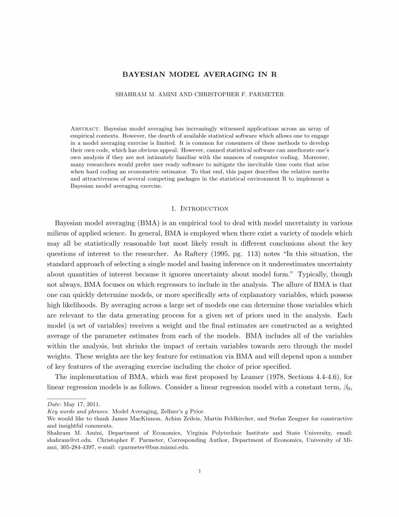
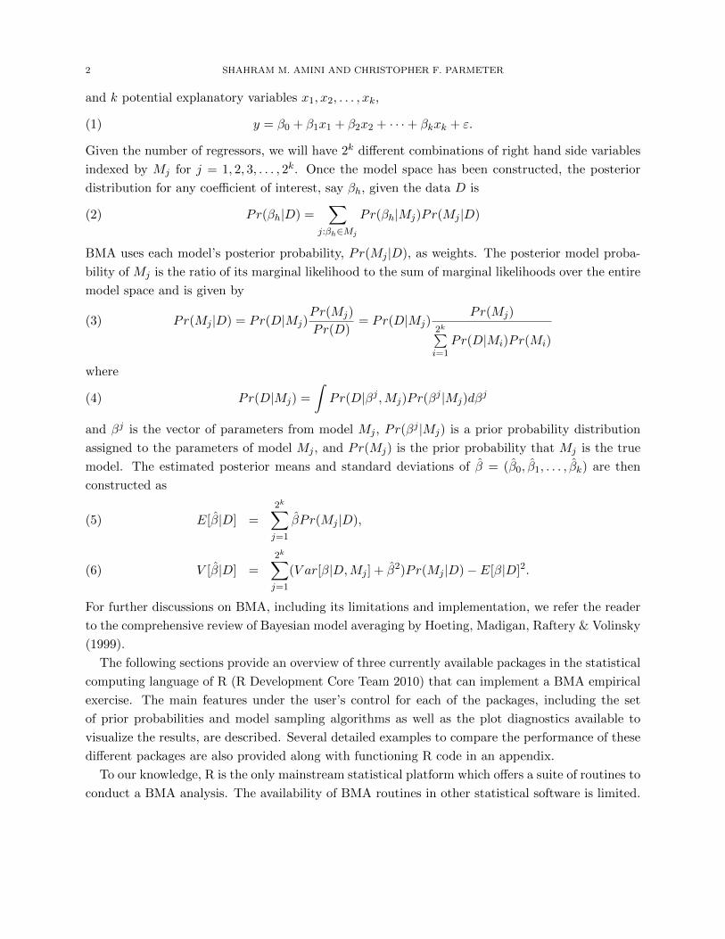
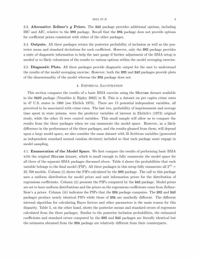
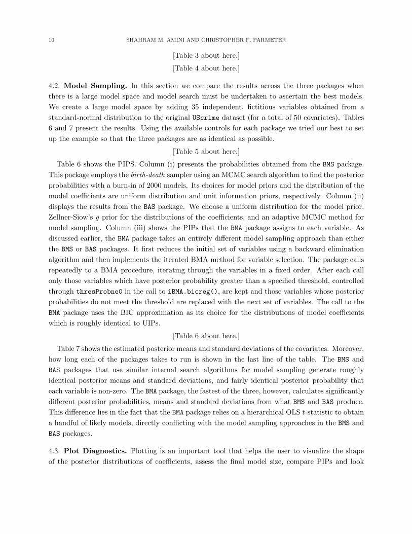
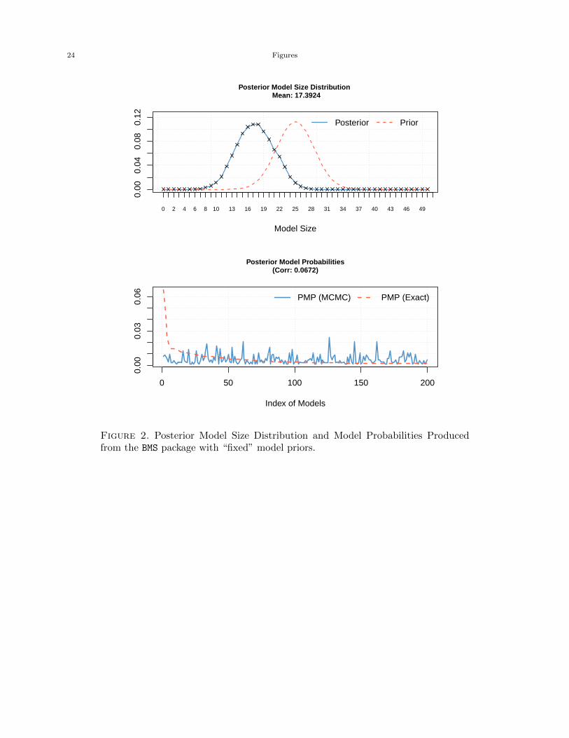
Figures 1 and 2 are combined plots provided by the BMS package. The upper plot in each figure
shows the prior and posterior distribution of model sizes and helps to illustrate to the user the
impact of the model prior assumption on the estimation results. Consistent with the research of
Ley & Steel (2009) and Eicher, Papageorgiou & Raftery (2011), who stress the importance of model
priors in applied work, the plots produced by the BMS package allow for visual clarification of choice
of model prior on posterior results. For example, the upper plot of Figure 1 assumes a uniform
distribution for the model prior whereas the upper plot of Figure 2 assumes a “fixed” common prior
inclusion probability for each regressor as an alternative to a uniform prior.13 These plots allow
the user to graphically compare across a range of model size priors to determine the impact on the
posterior distribution. In the example here it seems that the model prior (either fixed or uniform)
has little effect on the posterior distribution of model sizes.
[Figure 2 about here.]
The lower plot of both figures shows the analytical likelihood of the best 200 models and their
MCMC frequencies/draws of these models from the MCMC sampler. If the sampler has converged,
then the MCMC draws should conform to the analytical/exact likelihoods. This is expressed in
the correlation of the two lines by the correlation reported in parentheses beneath the plot’s title.
In other words, these graphs are an indicator of how well the current 200 best models encountered
by the search algorithm of the BMS package have converged. These plots are useful in determining
the search mechanisms ability to find ‘good’ models throughout the model space. If the user deems
that the best models are not acceptable then longer runs of the search algorithm or more burn-ins
may be specified to help refine the search over the model space.
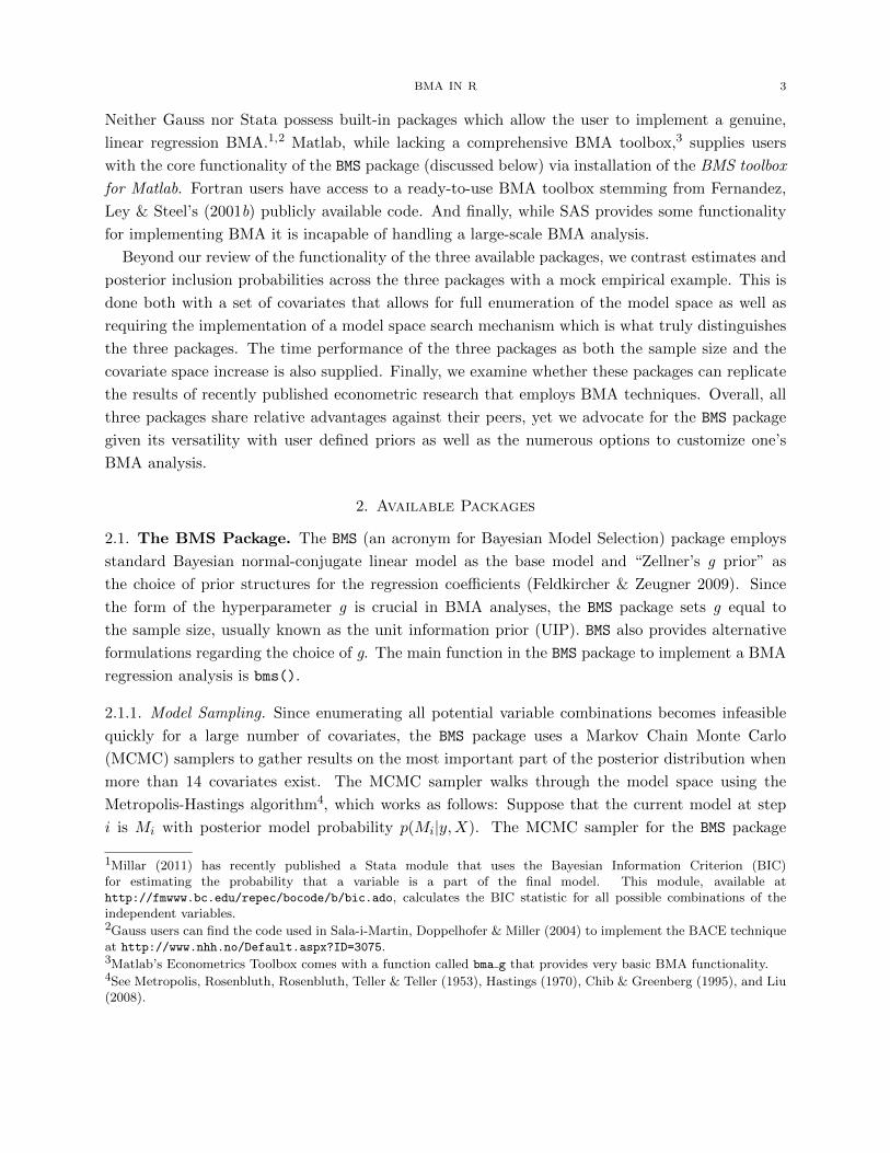
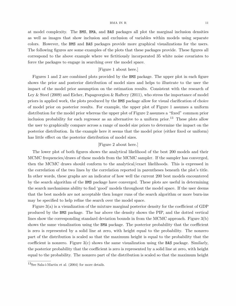
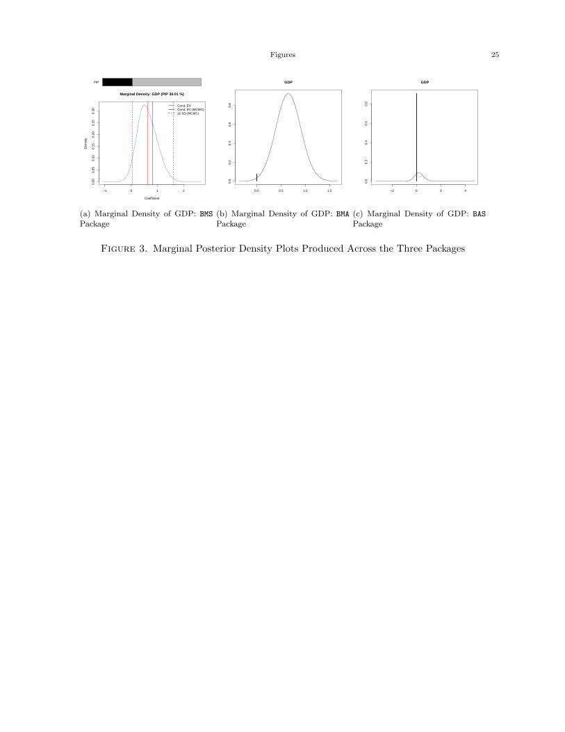
Figure 3(a) is a visualization of the mixture marginal posterior density for the coefficient of GDP
produced by the BMS package. The bar above the density shows the PIP, and the dotted vertical
lines show the corresponding standard deviation bounds in from the MCMC approach. Figure 3(b)
shows the same visualization using the BMA package. The posterior probability that the coefficient
is zero is represented by a solid line at zero, with height equal to the probability. The nonzero
part of the distribution is scaled so that the maximum height is equal to the probability that the
coefficient is nonzero. Figure 3(c) shows the same visualization using the BAS package. Similarly,
the posterior probability that the coefficient is zero is represented by a solid line at zero, with height
equal to the probability. The nonzero part of the distribution is scaled so that the maximum height
13See Sala-i-Martin et al. (2004) for more details.
12 SHAHRAM M. AMINI AND CHRISTOPHER F. PARMETER
is equal to the probability that the coefficient is nonzero. We mention here that Figure 3(b) is the
only plot produced within the BMA package.
[Figure 3 about here.]
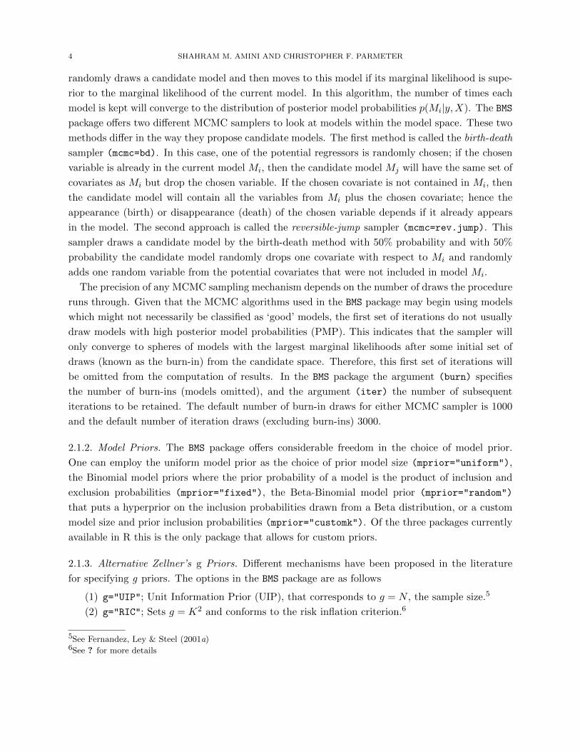
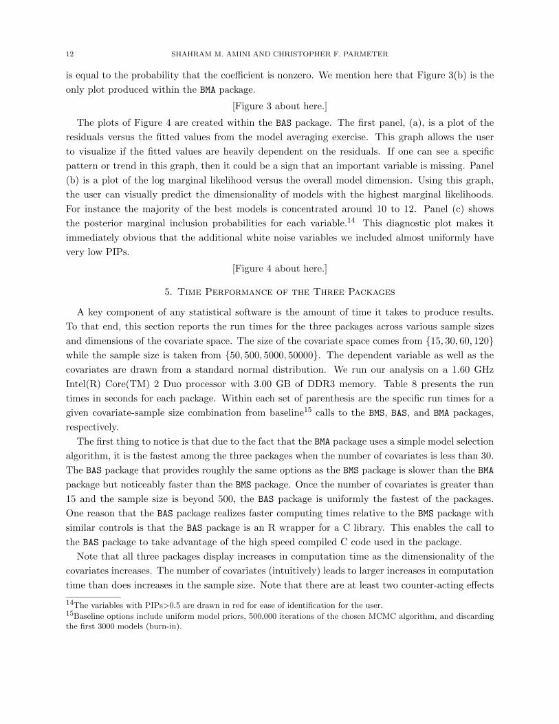
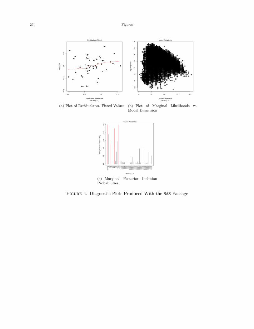
The plots of Figure 4 are created within the BAS package. The first panel, (a), is a plot of the
residuals versus the fitted values from the model averaging exercise. This graph allows the user
to visualize if the fitted values are heavily dependent on the residuals. If one can see a specific
pattern or trend in this graph, then it could be a sign that an important variable is missing. Panel
(b) is a plot of the log marginal likelihood versus the overall model dimension. Using this graph,
the user can visually predict the dimensionality of models with the highest marginal likelihoods.
For instance the majority of the best models is concentrated around 10 to 12. Panel (c) shows
the posterior marginal inclusion probabilities for each variable.14 This diagnostic plot makes it
immediately obvious that the additional white noise variables we included almost uniformly have
very low PIPs.
[Figure 4 about here.]
5. Time Performance of the Three Packages
A key component of any statistical software is the amount of time it takes to produce results.
To that end, this section reports the run times for the three packages across various sample sizes
and dimensions of the covariate space. The size of the covariate space comes from {15, 30, 60, 120}while the sample size is taken from {50, 500, 5000, 50000}. The dependent variable as well as the
covariates are drawn from a standard normal distribution. We run our analysis on a 1.60 GHz
Intel(R) Core(TM) 2 Duo processor with 3.00 GB of DDR3 memory. Table 8 presents the run
times in seconds for each package. Within each set of parenthesis are the specific run times for a
given covariate-sample size combination from baseline15 calls to the BMS, BAS, and BMA packages,
respectively.
The first thing to notice is that due to the fact that the BMA package uses a simple model selection
algorithm, it is the fastest among the three packages when the number of covariates is less than 30.
The BAS package that provides roughly the same options as the BMS package is slower than the BMA
package but noticeably faster than the BMS package. Once the number of covariates is greater than
15 and the sample size is beyond 500, the BAS package is uniformly the fastest of the packages.
One reason that the BAS package realizes faster computing times relative to the BMS package with
similar controls is that the BAS package is an R wrapper for a C library. This enables the call to
the BAS package to take advantage of the high speed compiled C code used in the package.
Note that all three packages display increases in computation time as the dimensionality of the
covariates increases. The number of covariates (intuitively) leads to larger increases in computation
time than does increases in the sample size. Note that there are at least two counter-acting effects
14The variables with PIPs>0.5 are drawn in red for ease of identification for the user.15Baseline options include uniform model priors, 500,000 iterations of the chosen MCMC algorithm, and discardingthe first 3000 models (burn-in).
BMA IN R 13
as the sample size, n, increases. A larger n puts more posterior mass on the best models. Therefore
we expect that the MCMC sampler will converge quicker. On the other hand, the larger n, the more
‘large’ models will be emphasized, which slows down the sampler. If these two effects offset each
other then we expect little change in run time over n. This is apparent in the BMS package. Notice
how the BMS package has run times which decrease for a fixed level of covariates as we increase n
while both the BAS and BMA packages actually take longer for n = 50, 000 relative to n = 5, 000.
[Table 7 about here.]
6. Replicability
In this section we examine the ability of these three packages in replicating the results of published
work research deploying BMA using handwritten code. Fernandez et al. (2001b) (FLS hereafter)
use a cross section of 72 countries along with 41 potential growth determinants for the period 1960
to 1992.16 FLS apply BMA to find the key determinants of economic growth given the numerous
plausible models that have emerged on the topic. We use the same dataset and deploy all three
BMA packages, BMS, BAS, and BMA, to attempt to replicate their results. In order to maximize
our opportunity to replicate the FLS results, we set the available options within each of the three
packages as close as possible to the specifications listed in FLS. The BMS package applies the MCMC
algorithm to search over the model space, burns the first 100,000 models and the number of iteration
draws to be sampled by its MCMC sampler is 200,000. It assigns the uniform distribution to the
model priors. Similarly, the BAS package employs MCMC method to walk through the model space,
discards the first 100,000 models, draws samples from the model space 200,000 times, and sets the
models priors to the uniform distribution. The BMA package, on the other hand, does not have
enough options to directly mimic the setup in FLS (see sections 2.4 and 3.1). Having said this, we
set the number of iteration draws used by its search algorithm to 200,000, the maximum ratio for
excluding models in Occam’s window, OR, to 20 and keep the the maximum number of columns in
the design matrix at the default of 31.
[Table 8 about here.]
Table 9 shows the PIPs for the variables of interest. We do not present posterior means or
standard deviations since FLS only reported the PIPs in the body of their paper. To eschew
making statements regarding results which FLS did not cover, we focus exclusively on the ability
of the packages to reproduce the PIPs found in FLS. Column (i) shows the published PIPs that
Fernandez et al. (2001b) have reported in their work and the remainder of table presents the PIPs
computed via the BMS, BAS, and BMA packages.
As is apparent, only the BMS package is reasonably successful at matching the reported PIPs
in FLS while the PIPs produced by the BAS package display significant differences (compare PIPs
marked by *). The BMA package also fails achieve the same PIPs of FLS.17 This most likely lies
16This dataset is taken from the larger dataset used by Sala-i-Martin (1997) for his study on robust determinants ofgrowth. The exact FLS dataset is publicly available on the Journal of Applied Econometrics online data archive.17Both BAS and BMA, however, are computationally much faster than the BMS package.
14 SHAHRAM M. AMINI AND CHRISTOPHER F. PARMETER
in the fact that the BMA package was not called using exactly the setup in FLS and the difference
in searching the model space that was described earlier. Interestingly, the PIPs returned from the
BMS package almost uniformly match FLS’ PIPs greater than 0.5. A key distinction between the
results is that both the BAS and BMA packages suggest a set of variables that belong in the final
model (PIP> 0.5) beyond those found in FLS. Specifically, the BAS package finds 13 variables with
PIPs > 0.5 beyond FLS (and one variable with PIP < 0.5 from FLS) while the BMA package finds
10 variables with PIPs > 0.5 (and one variable with PIP < 0.5 from FLS).
To further test the limits of these packages to replicate published results on BMA we attempt to
reproduce the estimates in Doppelhofer & Weeks’s (2009) research, (hereafter DW), who focused
on the use of model averaging when jointness of the covariates is considered. DW’s application
is identical to FLS, studying the determinants of economic growth. Appendix B of their paper
provides the BMA PIPs which we try to replicate using the ensemble of BMA packages. The data
used in DW comprises 88 countries and 67 candidate variables as a cross section for the period
1960 to 1996. The definition of all 67 variables used can be found in data appendix B in DW and
the dataset is publicly available on the Journal of Applied Econometrics data archive. As before
we have tried to preserve the setup in DW by setting the packages’ options as identical as possible.
[Table 9 about here.]
Table 10 displays our findings. Column (i) shows the published PIPs> 0.50 that DW report in
Appendix B of their paper. The rest of table presents the PIPs, posterior means and standard
deviations from each of the packages.18 The results indicate that the BMS package is the only
one that successfully reproduces the reported PIPs and posterior mean/standard deviation. Both
the BAS and BMA packages reasonably reproduce the posterior means/standard deviations but the
computed PIPs are significantly different from the published PIPs. For instance, the probability
that “Investment Price” belongs to the final model is roughly 77% according to DW but the BAS
packages reports this probability at nearly 7% and the BMA package reports it at exactly 100%!
The estimated coefficients are reasonably close for all packages yet there remain some anomalies.
The estimated posterior mean on Fraction of Tropical Area in the BMS package is about a third
as small as that reported from the BAS package and half the size of the reported posterior mean
from the BMA package. Moreover, both the BAS and BMA packages are suggestive that Fraction of
Tropical Area is relevant from a pure t-ratio perspective (see Masanjala & Papageorgiou 2008).
Beyond differences in several of the posterior means across the packages the standard deviations
show noticeable differences; compare the results for Investment Price where the standard deviation
from the BMS package is nearly double that from the BMA package and almost five times as large
from the reported standard deviation in the BAS package.
18DW do not report estimated posterior means or standard deviations.
BMA IN R 15
7. Conclusions
This paper has outlined the currently available BMA packages (BMS, BAS, and BMA) in the statis-
tical computing environment R. Our goal was to familiarize users with the different options that the
current versions of the packages have to offer. We highlighted how each of the packages implements
a BMA analysis as well as the options available to the user and the outputs that are returned.
To further cement the operation of these packages and to determine how similar the packages are
in practice, we presented a simple empirical example that first allowed all three packages to fully
enumerate the model space. Beyond this we enhanced our empirical example to force all three
packages to engage in search mechanisms throughout the model space. When the model space
is relatively small, we see that all three packages are successful at matching the PIPs, posterior
means, and posterior standard deviations. However, for the larger model space similarity of the
PIPs broke down considerably.
To further buttress our investigation and comparison of these packages we also compared runtimes
of generic calls to each package for a range of covariate and sample sizes. In most instances the BAS
package was the fastest, especially for large problems (both in terms of the number of covariates
and the number of observations). Additionally, we also sought to replicate two recent studies that
deployed BMA to investigate the determinants of economic growth. Both of these studies used
high level programming outside of R and as such represent the perfect opportunity to see how well
these freely available packages compare to computer code specifically tailored to the problem at
hand. Our results were striking. The BMS package almost exactly reproduced the results from both
studies while the BAS and BMA packages were not able to match the reports PIPS in either study
but were reasonably accurate at constructing the posterior means and standard deviations of our
second study (compared with the same estimates from the BMS package).
In sum, it appears that while the BMS package is invariably slower than its peers, its numerous
options and flexibility suggest that it should makes its way into the toolkit of applied researchers
seeking to use BMA in their analysis. The results from the empirical examples from published
studies suggest that while both the BMS and BAS packages offer a similar array of options, the BMS
package is capable of replicating published studies deploying BMA at the cost of slightly longer
run times. Our apparent advocacy of the BMS package does not hinge on its ability to reproduce
the results of published studies however, as this presumably just means that the original authors
used an implementation similar to that of the BMS package which the other packages were unable to
match. This in no way is an indicator of superiority. Lastly, the relative rigidity of the BMA package
to that of both BMS and BAS suggests that its use in applied work should be carefully scrutinized.
16 SHAHRAM M. AMINI AND CHRISTOPHER F. PARMETER
References
Chib, S. & Greenberg, E. (1995), ‘Understanding the Metropolis-Hastings algorithm’, American Statistician
49(4), 327–335.
Clyde, M. (2010), BAS: Bayesian Adaptive Sampling for Bayesian Model Averaging. R package version 0.92.
URL: http://CRAN.R-project.org/package=BAS
Clyde, M., Ghosh, J. & Littman, M. (2010), ‘Bayesian adaptive sampling for variable selection and model averaging’,
Journal of Computational and Graphical Statistics, to appear .
Doppelhofer, G. & Weeks, M. (2009), ‘Jointness of growth determinants’, Journal of Applied Econometrics 24(2), 209–
244.
Ehrlich, I. (1973), ‘Participation in illegitimate activities: A theoretical and empirical investigation’, The Journal of
Political Economy 81(3), 521–565.
Eicher, T. S., Papageorgiou, C. & Raftery, A. E. (2011), ‘Default priors and predictive performance in Bayesian model
averaging with application to growth determinants’, Journal of Applied Econometrics 26, 30–55.
Feldkircher, M. & Zeugner, S. (2009), Benchmark Priors Revisited: On Adaptive Shrinkage and the Supermodel
Effect in Bayesian Model Averaging, IMF Working Papers 09/202, International Monetary Fund.
URL: http://ideas.repec.org/p/imf/imfwpa/09-202.html
Fernandez, C., Ley, E. & Steel, M. (2001a), ‘Benchmark priors for Bayesian model averaging’, Journal of Econometrics
100(2), 381–427.
Fernandez, C., Ley, E. & Steel, M. (2001b), ‘Model uncertainty in cross-country growth regressions’, Journal of
Applied Econometrics 16(5), 563–576.
Furnival, G. & Wilson Jr, R. (1974), ‘Regressions by Leaps and Bounds’, Technometrics 16(4), 499–511.
George, E. & Foster, D. (2000), ‘Calibration and empirical Bayes variable selection’, Biometrika 87(4), 731–747.
Hastings, W. (1970), ‘Monte Carlo sampling methods using Markov chains and their applications’, Biometrika
57(1), 97–109.
Hoeting, J., Madigan, D., Raftery, A. & Volinsky, C. (1999), ‘Bayesian model averaging: A tutorial’, Statistical
science 14(4), 382–401.
Leamer, E. (1978), Specification searches: Ad hoc inference with nonexperimental data, Wiley New York.
Ley, E. & Steel, M. (2009), ‘On the effect of prior assumptions in Bayesian model averaging with applications to
growth regression’, Journal of Applied Econometrics 24(4), 651–674.
Liang, F., Paulo, R., Molina, G., Clyde, M. & Berger, J. (2008), ‘Mixtures of g priors for Bayesian variable selection’,
Journal of the American Statistical Association 103(481), 410–423.
Liu, J. (2008), Monte Carlo strategies in scientific computing, Springer Verlag.
Masanjala, W. & Papageorgiou, C. (2008), ‘Rough and Lonely Road to Prosperity: A reexamination of the sources
of growth in Africa using Bayesian Model Averaging’, Journal of Applied Econometrics 23(5), 671–682.
Metropolis, N., Rosenbluth, A., Rosenbluth, M., Teller, A. & Teller, E. (1953), ‘Equation of state calculations by fast
computing machines’, The Journal of Chemical Physics 21(6), 1087–1092.
Millar, P. (2011), ‘BIC: Stata module to evaluate the statistical significance of variables in a model’, Statistical
Software Components, Boston College Department of Economics.
URL: http://econpapers.repec.org/RePEc:boc:bocode:s449507
R Development Core Team (2010), R: A Language and Environment for Statistical Computing, R Foundation for
Statistical Computing, Vienna, Austria. ISBN 3-900051-07-0.
URL: http://www.R-project.org
Raftery, A. E. (1995), ‘Bayesian model selection in social research’, Sociological Methodology 25, 111–163.
BMA IN R 17
Raftery, A., Hoeting, J., Volinsky, C., Painter, I. & Yeung, K. Y. (2010), BMA: Bayesian Model Averaging. R package
version 3.13.
URL: http://CRAN.R-project.org/package=BMA
Sala-i-Martin, X. (1997), ‘I just ran two million regressions’, The American Economic Review 87(2), 178–183.
Sala-i-Martin, X., Doppelhofer, G. & Miller, R. (2004), ‘Determinants of long-term growth: A Bayesian averaging of
classical estimates (BACE) approach’, American Economic Review 94(4), 813–835.
Strawderman, W. (1971), ‘Proper Bayes minimax estimators of the multivariate normal mean’, The Annals of Math-
ematical Statistics 42(1), 385–388.
Venables, W. N. & Ripley, B. D. (2002), Modern Applied Statistics with S, fourth edn, Springer, New York. ISBN
0-387-95457-0.
URL: http://www.stats.ox.ac.uk/pub/MASS4
Zellner, A. & Siow, A. (1980), ‘Posterior odds ratios for selected regression hypotheses’, Trabajos de Estadıstica y de
Investigacion Operativa 31(1), 585–603.

18 SHAHRAM M. AMINI AND CHRISTOPHER F. PARMETER
Appendix A. R codes to produce tables results
We used the following codes to generate the results shown in the tables.
# Loading datasets and required libraries
#########################################
set.seed(2011)
library(MASS)
data(UScrime); attach(UScrime)
UScrime1 <- (cbind(log(UScrime[,c(16,1,3:15)]), So))
noise<- matrix(rnorm(35*nrow(UScrime)), ncol=35)
colnames(noise)<- paste(’noise’, 1:35, sep=’’)
UScrime.log <- cbind(UScrime1,noise)
X <- UScrime1[,-1]; Y <- UScrime1[,1]
x <- UScrime.log[,-1]; y <- UScrime.log[,1]
# Full enumaration of model space (Tables 4 and 5)
##################################################
# BMS Package:
library(BMS)
bms_enu <- bms(UScrime1, mcmc="enumerate", g="UIP", mprior="uniform",
user.int=FALSE)
coef(bms_enu)
detach("package:BMS")
# BMA Package:
library(BMA)
bma_enu <- iBMA.bicreg(X, Y, thresProbne0 = 5, verbose = TRUE, maxNvar = 30)
summary(bma_enu)
detach("package:BMA")
# BAS Package:
library(BAS)
bas_enu<- bas.lm(y~., data=UScrime1, n.models=NULL, prior="ZS-null",
modelprior=uniform(), initprobs="Uniform")
BMA IN R 19
coef(bas_enu)
detach("package:BAS")
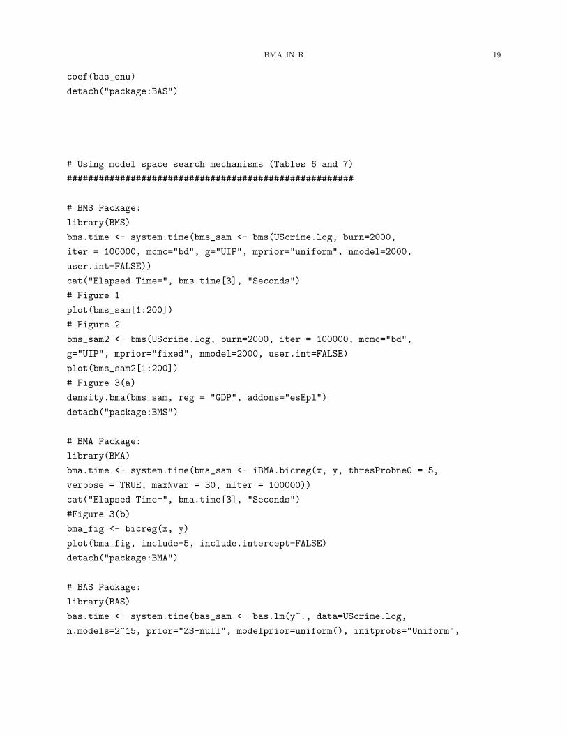
# Using model space search mechanisms (Tables 6 and 7)
######################################################
# BMS Package:
library(BMS)
bms.time <- system.time(bms_sam <- bms(UScrime.log, burn=2000,
iter = 100000, mcmc="bd", g="UIP", mprior="uniform", nmodel=2000,
user.int=FALSE))
cat("Elapsed Time=", bms.time[3], "Seconds")
# Figure 1
plot(bms_sam[1:200])
# Figure 2
bms_sam2 <- bms(UScrime.log, burn=2000, iter = 100000, mcmc="bd",
g="UIP", mprior="fixed", nmodel=2000, user.int=FALSE)
plot(bms_sam2[1:200])
# Figure 3(a)
density.bma(bms_sam, reg = "GDP", addons="esEpl")
detach("package:BMS")
# BMA Package:
library(BMA)
bma.time <- system.time(bma_sam <- iBMA.bicreg(x, y, thresProbne0 = 5,
verbose = TRUE, maxNvar = 30, nIter = 100000))
cat("Elapsed Time=", bma.time[3], "Seconds")
#Figure 3(b)
bma_fig <- bicreg(x, y)
plot(bma_fig, include=5, include.intercept=FALSE)
detach("package:BMA")
# BAS Package:
library(BAS)
bas.time <- system.time(bas_sam <- bas.lm(y~., data=UScrime.log,
n.models=2^15, prior="ZS-null", modelprior=uniform(), initprobs="Uniform",
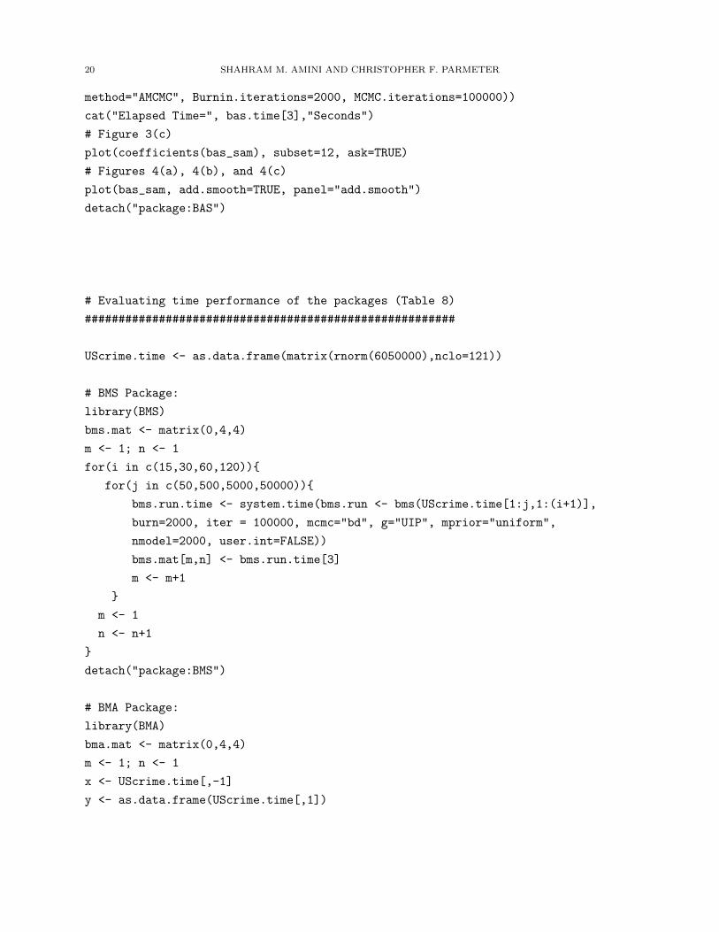
20 SHAHRAM M. AMINI AND CHRISTOPHER F. PARMETER
method="AMCMC", Burnin.iterations=2000, MCMC.iterations=100000))
cat("Elapsed Time=", bas.time[3],"Seconds")
# Figure 3(c)
plot(coefficients(bas_sam), subset=12, ask=TRUE)
# Figures 4(a), 4(b), and 4(c)
plot(bas_sam, add.smooth=TRUE, panel="add.smooth")
detach("package:BAS")
# Evaluating time performance of the packages (Table 8)
#######################################################
UScrime.time <- as.data.frame(matrix(rnorm(6050000),nclo=121))
# BMS Package:
library(BMS)
bms.mat <- matrix(0,4,4)
m <- 1; n <- 1
for(i in c(15,30,60,120)){
for(j in c(50,500,5000,50000)){
bms.run.time <- system.time(bms.run <- bms(UScrime.time[1:j,1:(i+1)],
burn=2000, iter = 100000, mcmc="bd", g="UIP", mprior="uniform",
nmodel=2000, user.int=FALSE))
bms.mat[m,n] <- bms.run.time[3]
m <- m+1
}
m <- 1
n <- n+1
}
detach("package:BMS")
# BMA Package:
library(BMA)
bma.mat <- matrix(0,4,4)
m <- 1; n <- 1
x <- UScrime.time[,-1]
y <- as.data.frame(UScrime.time[,1])
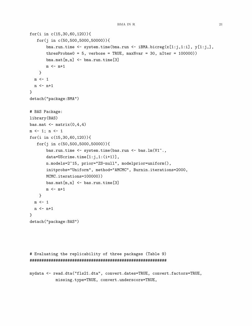
BMA IN R 21
for(i in c(15,30,60,120)){
for(j in c(50,500,5000,50000)){
bma.run.time <- system.time(bma.run <- iBMA.bicreg(x[1:j,1:i], y[1:j,],
thresProbne0 = 5, verbose = TRUE, maxNvar = 30, nIter = 100000))
bma.mat[m,n] <- bma.run.time[3]
m <- m+1
}
m <- 1
n <- n+1
}
detach("package:BMA")
# BAS Package:
library(BAS)
bas.mat <- matrix(0,4,4)
m <- 1; n <- 1
for(i in c(15,30,60,120)){
for(j in c(50,500,5000,50000)){
bas.run.time <- system.time(bas.run <- bas.lm(V1~.,
data=UScrime.time[1:j,1:(i+1)],
n.models=2^15, prior="ZS-null", modelprior=uniform(),
initprobs="Uniform", method="AMCMC", Burnin.iterations=2000,
MCMC.iterations=100000))
bas.mat[m,n] <- bas.run.time[3]
m <- m+1
}
m <- 1
n <- n+1
}
detach("package:BAS")
# Evaluating the replicability of three packages (Table 9)
##########################################################
mydata <- read.dta("fls21.dta", convert.dates=TRUE, convert.factors=TRUE,
missing.type=TRUE, convert.underscore=TRUE,
22 SHAHRAM M. AMINI AND CHRISTOPHER F. PARMETER
arn.missing.labels=TRUE)
bmadata <- mydata[,-2]
y <- bmadata[,1] ; x <- bmadata[,-1]
attach(bmadata)
library(BMS)
bms.time <- system.time(fls.bms <- bms(bmadata, burn=10000,
iter=500000, g="UIP", mprior="uniform", nmodel=3000, mcmc="bd",
ser.int=FALSE))
coef(fls.bms)
detach("package:BMS")
library(BAS)
bas.time <- system.time(fls.bas <- bas.lm(gr56092~., data=bmadata,
n.models=2^15, prior="ZS-null", modelprior=uniform(), initprobs="Uniform",
method="AMCMC", Burnin.iterations=10000, MCMC.iterations=500000))
coef(fls.bas)
detach("package:BAS")
library(BMA)
bma.time <- system.time(fls.bma<- iBMA.bicreg(x, y, thresProbne0 = 5,
verbose = TRUE, maxNvar = 30, nIter = 500000))
summary(fls.bma)
detach("package:BMA")
################################## END ##################################

Figures 23
0.00
0.04
0.08
0.12
Posterior Model Size Distribution Mean: 17.4396
Model Size
0 2 4 6 8 10 13 16 19 22 25 28 31 34 37 40 43 46 49
Posterior Prior
0 50 100 150 200
0.00
0.02
0.04
Posterior Model Probabilities(Corr: −0.1133)
Index of Models
PMP (MCMC) PMP (Exact)
Figure 1. Posterior Model Size Distribution and Model Probabilities Producedfrom the BMS package with “uniform” model priors.
24 Figures
0.00
0.04
0.08
0.12
Posterior Model Size Distribution Mean: 17.3924
Model Size
0 2 4 6 8 10 13 16 19 22 25 28 31 34 37 40 43 46 49
Posterior Prior
0 50 100 150 200
0.00
0.03
0.06
Posterior Model Probabilities(Corr: 0.0672)
Index of Models
PMP (MCMC) PMP (Exact)
Figure 2. Posterior Model Size Distribution and Model Probabilities Producedfrom the BMS package with “fixed” model priors.
Figures 25
PIP
−1 0 1 2
0.00
0.05
0.10
0.15
0.20
0.25
0.30
Marginal Density: GDP (PIP 30.01 %)
Coefficient
Den
sity
Cond. EVCond. EV (MCMC)2x SD (MCMC)
(a) Marginal Density of GDP: BMS
Package
0.0 0.5 1.0 1.5
0.0
0.2
0.4
0.6
0.8
GDP
(b) Marginal Density of GDP: BMA
Package
−2 0 2 4
0.0
0.2
0.4
0.6
0.8
GDP
(c) Marginal Density of GDP: BAS
Package
Figure 3. Marginal Posterior Density Plots Produced Across the Three Packages
26 Figures
6.0 6.5 7.0 7.5
−0.
4−
0.2
0.0
0.2
Predictions under BMA
Res
idua
ls
●
●
●
●
●
●
●
●
●
●
●
●
●
●
●
●
●
●
●
●
●
●
●
●
●
●
●
●
●
●
●
●
●
●
●
●
●●
●
●
●
●
●
●
●
●
●
bas.lm(y ~ .)
Residuals vs Fitted
22 46
11
(a) Plot of Residuals vs. Fitted Values
●●
● ●●
●
●●●
●●
●
●● ●
●●
●●●●●
●●
●●●●
●
●●
●
●
●●
●
●
● ●●● ●
●
● ●
●●
●
●●●
●● ● ●●
●●
●● ●● ●
●
●
●●●●●●
●●●●●
●
●●●●●
●
●●
● ●
●
●●●
●●●
●●●
●●
●●
● ●●● ●
●
●●●●●●
●
●
●●●
●●
●●
●●●
●●
●●●●●●
●●●●●
●●●
●●●●
●●
●●
●●
● ●
●●● ●
●●● ●●
●● ●●
●
●●
●
●
●●
●●
●
●
●
●
●●
●
●
●●
●
●●
●●●●
●●
●●●●●●
●●●
●●●
●●●
●●●●
●●
●●●●●●
●●
●
●● ● ●
●●
●●●●
●
●
●
●
●
●●
●●●
●
●
●●
●
●●●●
●●
●
●●
●
●
●
●●●
●●
●●
●●
●
●
●●●●●●
●●●●
● ●●
●●
●●
●
●
●
●
●
●●
●
●●
●● ●
● ●
●
●
● ●●
●●
●●
●●
●●●●●● ●●
●●
●●●●●●
●●
●●
●●
●●● ●
●●
●
●● ●
● ●●
●
●●
●●
●●●
●
●
●●
●
●●
●●●
●●●●
●●●●●
●●
●●●
●
●
●
●
●●
●● ●●●
●
●●●
●●●
●
●●● ●
●●
●
●●
●●
●
●●
●
●●●●
●
●●● ● ●
●
●●●●
●●
●●●●●
●
●
●●
●●
●●
●●● ● ●
●
●●
●
●●
●●
●●
● ●
●●●
●
●●
●●●●
●
●●
●●
●●
●●●●●●●
●
●●
●●●
●
● ●
● ●
●
●
●●
●
●
●●
●●●
●
●● ●●●
●
●
●●
●●●●● ●●
●
●
●
●
●●
●
●●
●●
●●●
●●
●
●●●
●●●
●
●●
●
●●●
●●●
●●
●●
●
●●●
●●●●
●
●●
●●
●●
●●
●
●
●
●
●
●●●
●
●●●●●●
●●●
●●●● ●
●●
●●●●●
●●
●●
●
●●
●
●●●
●●●●
●●
●●● ●●
●
●
●
●
●●●●●
●
●●
●
●
●● ●●●
●
●●
●●
●●
●
●● ●
●●
●●
●
●
●●●
●●●●
●
●●
●
●●●●
●
●●
●
●●● ●●
●
●
●●● ●
●●●
●
●
●●●
●●● ●●
●
●
●●
●
●
●●
●●●
●●
●●●
●
●
●
●●●
●●●● ●●●●●
●●
●●●
●●
●●
●●●
●●
●●
●
●●●●
●
●●●●●
●
●
●●●● ●
●●●●
●
●●●
●
● ●● ●
●●
●
●
●●●●●
●●
● ●●●
●
●● ●
●
●●●
●
●●
●●●
●●●●
●
●
●
●●
●
●●
●●●●●
●
●●●●
●
●●●●
●
●●●●
●
●●●●●
●
●
●
●●●●
●●
●●
●●
●
●
●●●
●
●●●
●●●●
●
●●
●
●●
●●●●●
●● ●●●● ●
● ●
●●
●
●●●
●
●
●
●
●●●●●●
●●
●●●
●●●●
●●●●●
●●
●
● ●
●●
●●●
●
●●
●
●●●●
●
●
●●
●●
●
●
●●●●
●
●●●
●●
●●
●
●
●●
●●●●●
● ●
●●
●
●●
●
●
●●●
●
●
●
●●
●●
●
●
● ●
●
●●
●
●●
●
●
●
●●
● ●
●
●
●
●
●
●
●
● ●●
●
●
●
●
●
●
●
●
●
●
●
●●
●
●
●
●●
●
●
●
●
●●
●
●
●
●
●●
●●
●
●
●●
●
●
●
● ●●
●
●
●
●
●
●●
●
●
●
●
●
●
●
●
●
●●●
●
●
●
●
●●
● ●
●
●
●
●
●
●
●
●
●
●●
●
●
● ●
●
●
●
●●
●●
●
●
●
●
●
●
●●
●
●●●
●
●
●
●
●
●
●
●
●
●
●
●
●
●
●
●●
●
●
●
●
●
●
●●
●
●
●
●
●
●
●
●
●
●
●
●
●
●
●
●●
●
●
●
●●
●
●
●●
●
●
●
●
● ●●
●
●
●
●
●
●
●
●●
●
●
●●
●
●
●●
●
●
●
●
●
●
●
●
●
●
●●
●
●●
●
●
●
●
●●
●●●
●
●
●
●●
● ●
●
●●
●
●
●
●
●
●
●
●
●
●
●
●
●
●
●●
●
●
●
●
●
●
●
●
●
●
●
●
●●
●
●
●
●
●●
●
●
●●
●
●
●
●
●
●
●
●
●
●
●●
●
●
●
●
●
●
●
●
●
●
●
●
●
●
●
●
●
●●
●
●
●
●
●
●
●
●
●
●
●
●
●
●
●
●
●
●●●●
●
● ●
●
●
●
●
●
●
●
●
●
●
●
●
●
●
●●
●●
●
●
●
●
●
●
●
●
●
●
●
●●
●
●
●
●
●
●
●
●
●
●
●
● ●
●
●
●
●
●
●
●
●
●
●
●
●
●
●
●
●
●●
●
●
●
●
●
●
●
●
●
●
●●
●
●
●
●
●
●
●
●
●
●
●
●
●
●
●
●
●
●
●
●
●●
●
●
●
●
●
●
●
●
●●
●
●
●
●
●
●
●
●
●
●
●●
●
●
●
●
●
●
●
●
●
●
●
● ●●
●
●
●
●
●
●
●●
●
●
●
●
●
●
●●
●
●
●
●
●
●
●
●
●
●
●
●● ●
●
●
●
● ●
●
●
●
●
●
●
●
●●
●
●
●
●●
●
●
●
●
●
●
●●
●
●
●
●●
●
●
●
●
●
●
●
●
●
●
●
●
●
●
●
●
●
●
●●
●●
●
●
●
●
●
●
●
●
●●
●
●
●
●●
●
●
●
●
●●
●
●
● ●
●
●
●●
●
●
●
●
●
●
●
●
●●
●●
●
●
●
●
●
●
●
●
●
●
●●
●
●
●
●
●
●
●
●●
●
●●
●
●
●
●
●
●
●
●
●
●
●●●
●
●
●
●
●
●●
●
●
●
●●
●
●
●●
●
●●
●
● ●
●
●
●●
●
●
●
●
●
●●
●
●
●
●
●
●
●
●
● ●
● ●
●
●●
●
●
●
●
●
●
●
●
●
●
●
●
●
●
●
●
●
●
●
●
● ●●
●
●
●●
●
●
●
●
●
●
●●
●
●
●
●
●
●
●
●
●
●
●
●
●
●
●
●
●
●
●
●
●
●●
●
●
●
●
●
●
●
●
●
●
●
●
●
●●
●
●
●
●●
●
●
●
●
●●
●
●
●
●
●
●
●
●
●
●
●●
●
●
●
●
● ●●
●
●
●
●
●
●
●●● ●
●
●
●●
●
●
●
●
●
●
●
●●
●●
●
●
●
●
●
●
●●
●
●
●
●
●
●●
● ●
●
●
●
●
●
●
●
●
●●
●●
●●
●
●●
●
●
●
●
●
●
●
●
●
●
●
●●
●
●
●
●
●●
●
●
●
●
●
●
●
●
●
●
●
●
●
●
●
●
●
●
●●
●
●
●
●
●
●
●
●
●
●
●
●
●
●
●
●
●
●
●
●
●
●●
●
● ●
●
●
●
●●
●
●
●
●
●
●
●
●
●
●
●
●
●
●●
●
●●
●
●
●
●
●
●●
●
●
●
●
●
●
● ●
●
●
●
●
●
●
●●
●
●
●
●
●●
●
●
●
●
●
●
●
●
●
●
●
●
●●●
●
●
●
● ●
●
●
●
●●
●
●
●
●
●
●
●
● ●
●●
●
●
●
●
●
●
●
●●●
●
●
●
●
●
●
●
●
●
●
●
●
●●
●●
●
●●
●
●
●
●
●
●●
●●
●
●●● ●
●
●
●
●
●
●●
●
●
●
●
●
●
●
●
●●
●●
●●
●
●
●
●
●
●●
●
●
●
●
●
●
●
●●
●
●
●●
●
●
●
●
●
●
●
●●
●
●
●●●
●
●
●
●
●
●
●
●
●
●
●
●
●
●
●
●
●
●
●
●●
●
●
●
●
●●
●
●
●
●
●
●
●
●
●
●
●
●
●
●
● ●
●
●
●●
●
●
●● ●●
●
● ●
●
●
●
●
●
● ●
●
●
●
●
●
●
●
●
●
●
●
●
●
●
●
●
●
●
●
●
●
●
●
●●
●
● ●
●
●
●
●
●
●
●
●
●
●
●
●
●
●
●●
●
●●
●
●
●●
●
●
●
●
●
●
●●
●
●
●
●
●
●
●
●
●
●●
●
●
●●
●
●
●●
●●
●
●
● ●●
●
●
●
●
●●
●
●
●
●
●
●
●
●
●
●
●
●
●
●
●
●
●
●
●
●
●
●
●
●●
●
●
●
●
●
●
●
●
●
●● ●
●
●
●
●
●
●
●
●
●
●
●
●●
●
●
●
●
●
●
●
●
●
●
●
●
●
●
●
●
● ●
●
●
●
●
●
●●
●
● ●
●
●
●●
● ●
●
●●
●
●●
●
●
●
●
●
●
●
●
●
●
●
●
●●
●
●
●
●
●
●
●
●
●
●
●
●
●
●●
●
●
●
●●
●
●
●
●●
●
●
●
●
●
●●
●
●
●
●
●
●
●
●
●
●
●
●
●
●
●●
●●
●
●
●
●
●
●
●
●
●
●●
●
●
●
●
●
●
●
●
●
●
●●
●
●
●
●
●
●
●
●●
●
●
●
●
●
●●
●
●
●
●
●
●
●
●
● ●
●
●
●
●
●●●
●
●
●●
●
●
●
●
●
●●
●
●
●
●●
●
●
●●
●
●
●
●
●
●●
●
●●●
●●
●
●
●●
●
●
●
●
●
●
●
● ●
●
●●
●
●
●
●
●
●
●
●●
●●
● ●
●
●
●
●●
●
●
●●
●
●
●
●
●
●●
●
●
●●
●●
●
●
●
●
●
●
●
●
●
●●
●
●
●
●
●
●
●
●
●
●
●
●
●
●
●
●●
●
●
●
●
● ●
●
●
●
●
●●
●
●
●
●
●
●●
●●● ●
●
●
●
●●
●
●
●
●
●
●
●
●●
●
●
●●
●
●
●●
●
●
●
●
●
●
●
●
●
●
●
●
● ●
●
●
●
●
●
●
●
●
●
●
● ●
● ●
●
●
●
●
●
●
●
●●
●
●
●
●
●
●●
●
●
●
●
●
●
●
●
●
●
●
●
●
●
●
●
●
●
● ●
●
●
●
●
●●
●●
●
●
●
●
● ●
●
●
●
●
●
●
● ●
●
●
●
●
●
●
●
●
●●
●
●
●
●
●
●
●
●
●
●
●
●
●
●
●
●
●
●●
●
●
●
●●
●●
●
●
●
●
●
●
●
●
●
●●
●
●
●
●
●
●
●
●
●
●
●
●
●●
●
●
●
●●
●
●
●
●
●
●
●
●
●
●
●
●
●
●
●
●
●
●
●
●●
●
●
●
●
●
●
●●
●
●
●
●
●
●
●
●
●●
●
●
●
●
●
●
●
●
●
●
●
●●
●●
●
●
●●
●
●
●
●
●
●●
●
●
●
●
●
●
●
●
●● ●
●
●
●
●
●
●
●
●
●
●
●
●●
●●
●
●
●
●
●●
●
●
●
●
●
●
●
●
●
●
●
●
●
●
●
●
●
●
●
●●
●
●
●
●
●
●●
●
●●
●
●
●
●
●
●●
●
●
●
●
●
●
●
●●
●
●
●
●
●
●
●
●●
●
●●
●
●
●
●
●
●
●
●
●
●
●
●
●
●
●●
●●
●
●
●
● ●
●
●
●
●●
●
●●
●
●
●●
●
●
●
●
●
●
●●
●
●
●●
●
●
●
●
●
●
●
●
●
●
●●
●
●
●
●
●
●
●
●
●
●
●
●
●●
●
●●
●●
●
●●
●
●
●
●
●
●
●
●
●
●
●
●
●●
●
●
●
●
●
●
●
●
●
●
●
●●
●
●
●
●●
●
●
●
●
●
●
●
●
●
●
●●
●
● ●
●
●
●
●
●●
●●
●
●
●
●
●
●● ●
●
●
●
●
●
●
●
●●
●
●
●
●
● ●
●
● ●
●
●
● ●●
●
●
●
●●
●
●
●
●
●
●
●●
●
●
●
●
● ●
●
●●
●
●
●
●
●
●
●
●
● ●
●
●
●
●
●
●
●
●●
●
●
●
●
●
●
●
●
●
●
●
● ●
●
●
●
●
●
●
●
●
●●
● ●
●
●
●
●
●
●●
●●
●
●
●
●
●
●
●
●
●
●
●●
●
●
●
●
●
●
●
●
●
●
●
●
●
●
●
●
●
●
●●
●
● ●
●
●
●
●
●
●
●
●
●●
●●
●
●
●
●
●
●
●
●
●
●
●
●
●
●
●
●
●
●
●
●
●
●
●
●
●
●
●
●
●
●
● ●
●
●
●
●
●●
●
●
●
●
●
●
●
●
●
●
● ●
●
●
●
●
●
●
●
●
●
●●
●●
●
●
●
●
●
●
●
●
● ●●
●
●
●
●
●
●
●
●
●●
●
●
●
●
●
●
●●
●
●
●
●
●● ●
●
●
●
●
●
●
●
●
●
●
●
●
●
●
●
●
●
●
●
●
●
●
●
●
●
●
●
●
●●
●
●
●
●
●
●
●
●
●
●
●
●
●
●
●●
●
●
● ●
●
●
●
●
●●
●
●
●●
●●
●
●
●
●
●
●
●
●
●
●
●
●
●
●
●
●
●●
●
●●
●
●●
●●
●
●
●●
●●
●
●
●
●
●
●
●
●●
● ●
●
● ●
●
●●
●
●
●
●●
●
● ●
●
●
●●
●
●
●
●
●
●
●●
●
●
●
●
●
●●●
●
●
●●
●
●
●●
●●
●
●
●
●
●
●
●
●
●
●
●
●
●
●
●
●
●
●
●●
●
●
●
●
●
●
●
●●
●
●●
●
●
●●
●
●●
●
●
●●
●
●
●
●
● ●
●
●●
●
●
●
●
●
●
●
●
●
●
●
●
●
●●
●
●
●
●
●●
●
●
●
●●
●
●●
●
●
●
●
●
●
●●
●●
●
●
●
● ●
●
●
●●
●
● ●
●
●●
●
●●
●
●
●
●
●
●
●●
●
●
●
●
●
●
●
●
●
●
● ●
●●
●
●
●●
●
●●
●
●
●
●
●
●
●●
●
●
●●
●●
●
●
●
●
●
●
●
●
●
●
●
●
●●
●
●
●
●
●
●●
●
●
●
●
●●
●
●
●
●
●
●
●
●
●
●
●●
●
●
●
●
● ●
●●
●
●
●
●
●
●●●
●
●
●
●
●
●
●
●
●
●
●●●
●
●
●
●
● ●
●
●
●
●
●●
●
● ●●
●
●
●
●
●
●
●
●●
●●
●
●
●
●
●
●
●
●●
●
●
●
●
●
●
●
●
●
● ●
●
●
●
●
●
●
●
●● ●
●
●
●
●
●
●
●●
●
●
●
●
●
●
●
●
●
●
●●
●
●
●
●●
●
●●
●
●●●
●●
●●
●
●
●
●
●●
●
●●
●
●
●
●●
●
●
●
●
● ●
●
●
●
●
●●
● ●
●
●
●
●
●
●
●●
●
●
●
●
●
● ●
●
●
●
●
●●
●
●
●●
●
●
●
●
●
●
●
●●
●●●●
●
●
●
●
●
●
●
●
● ●
●●
●●
●
●
●●
●
●
●●
●
●●
● ●
●
●
●
●
●
●
●
●
●
●
●
●
●
●
●
●
●
●
●
●
●
●
●
●●
●
● ●●
●
●
●
●
●
●●
●
●
●
●
●
●●
●
●
●
●
●
●
●●
●
●
●
●
●
● ●●
●
●
●
●
●
●●
●
●
●
●
●●
●
●●
●
●
●
●
●
●
●
●●
●
●
●●
●●
●
●
●
●
●
●●
●
●
●
●
●
●
●
●
●
●
●
●
●
●
● ●
●
●
●
●
●
●
●
●
●
●●
●
●
●
●
●
●
●
●
●●
●
●
●
●
●
●
●
●
●
●
●●
●
●●
●
●
●
●
●
●
●
●
●
●●
●
●
●
●
●●
●
●
●
●
●●
●●
●
● ●
●
●
●
●
●●
●
●
●
●
●
●
●
●
●
●
●
●
●
●
●
●
●
●
●●●
●
●
●
●
●
●
●●
●
●
●
●
●●
●
●
●
●●
●
●
●
●
●
●
●●
●
●
●
●
●
●
●
●
●
●
●
●
●
●
●
● ●
●
●
●
●●
●
●
●
● ●●●
●
●
●
●
●
●
●
● ●
●●
●
●
●
●
●
●
●
●
●
●
●
●
●
●
●
●
●
●
●
●
●
●
●
●●
●
●
●
●
●
●
●
●
●
●●
●
●
●
●
●
●
●●
●
●
●●
●
●
●
●
●
●
●
●
●●
●
●
●
●●
●
●
●
●
●
●
● ●
●
●●
●
●●
●
●●
●
●
●
●
●
●
●
●
●●
●
●
●●
●
●●●
●
●●
●
●
●
●●
●
●
●
●
●
●
●
●
●
●
●
●
●
●
●
● ●
●
●
●
●
●
●●
●
●
●●
●
●
●
●
●●
●
●
●
●
●
●
●
●
●
●●
●
●
●
●
●●
●
●
●
●●
●
●
●
●
●
●
●
●
●●
●
●
●
●
●
●
●
●
●
●
●
●
●●
●
●
●
●
●
●
●
●
●
●
●
●
●
●
● ●
●
●
●
●
●
●
●
●
●
●
●
●
●
●
●
●●
●
●
●●
●
●
●
●
●
●
●
●
●
●
●
●
●
●
●
●●
●
●
●
●
●
●
●
●
●
●
●●●
●
●
●
●
●
●
●
●
●
●●
●
●
●
●
●
●●●
●
●
●
●
●
●
●
●
●
●
●
●●●
●
●
●
●
●
●
●●
●
●
●
●
●
●
●
●
●
●
●
●●
●
●●
●
●
●
●
●
●
●●
●●
●
●
●
●●
●●
●
● ●●
●
●
●
●●
●
●
●
●
● ●
●
●
●
●
●●
●
●
●
●●
●
●
●
●
●
●
●
●
●
●
●
●
●
●
●
●
● ●●
●
●
●
●
●
●
●
●
●
●
●
●
●
●
●
●
●
●
●
●●
●
●
●
●
●
●
●
●
●●●
●
●
●
●
● ●
●
●
●
●●
●
● ●
●
●
● ●
●
●●
●
●
●
●
●
●
●
●
●
●
●
●
●
●
●
●
●
●
●
●
●
●
●
●●
●
●
●
●
●
●
●
●
●
●
●
●
●
●
●
●
●
●
●
●
●●
●
●
●
●
●
●
●
●
●
●
●
●
●
●
●●
●●
●
●
●
●
●
●
●
●●
●
●
●
●
●●
●
●
●
●
●
●●
●
●
●
●
●
●
●
●
●
●
●
●
●
●●
●
●
●●
●
●
●
●●
●
●
●
●
●
●
●
●
●●
●
●
●●
●
●
●
●
●
●● ●
●
●
●
●
●
●●
●
●
●
●
●
●
●
●
●
●
●●
●
●
●
●
●
●
●
●
●
●
●
●
●
●
●
●
●
●
●
●
●
●
●
●
●
●
●
● ●
●
●
●
●●
●
●
●
●
●
●
●●
●
●●
●
●
●
●●
●
●●
●
●
●
●
●
●●
●
●
●
●
●
●
●
●
●
●●
●
●
●
●
●
●
●
●
●
●
●
●
●
●
●
●
● ●
●
●
●
●●
●
●
●
●
●
●
●
●
●
● ●
●
●
●
●
●●●
●
●
●
●
●
●
●
●
●
●
●
●●
●
●
●
●
●
●
●
●
●
●
●
●
●
●
●
●
●
●
●
●
●
●
●
●
●
●
● ●●
●
●
●
●
●
●
●
●
●
●
●
●
●
●●
●
●
●
●
●
●
●
●
●
●
●
●
●
●
●
●
●
●
●
●
●
●
●
●
● ●
●
●
●
●
●
●
●●
●
●
●
●
●
●
●
●●
●●
●
●●
●
●
●
●
●
●●
●
●
●
●
●
●
●
●
●
●
●
●●
●
●
●
●
●
●
●
●
●
● ●
●●●
●
●
●
●
●
●
●●
●
●
●
●
●
●
●
●
●●
●
●
●
●
●
●
●
●
●
●
●
●
●
●
●
●●
●
●
●
●
●
●
●
●
●
●
●
●
●
●
●
●
●
●
●
●
●
●
● ●
●
●
●●
●
●
●
●
●
●
●
●
●
●
●●
●
●
●
●
●
●
●
●
●
●
●
●
●
●
●
●●
●
●
●
●●
●
● ●
●
●
●
●
●
●
●●
●●
●
●
●
●
●
●
●
●
●
●
● ●
●
●
●
●
●
● ●
●
●
●
●●
●
●
●
●
●
●
●
●
●
●
●
●
●
●
●●
●
●
●
●●
●
●
●● ●
●●
●
●
●
●
● ●
●
●●
●
●●
●
●
●
●
●
●● ●
●
●
●
●
●
●●
●
●●
● ●
● ●
●
●
●●
●
●●
●
●
●
●
●
●
●
●
●
●
●
●
●
●
●
●●
●●
●
●
●●
●
●●
●
● ●
●
●
●
●
●
●
●
●
●
●
●
●
●
●
●
●
●
●
●
●
●
●
●●
●
●
●
● ●
●
●
●
●
●
●
●
●
●
●
●
●
●
●
●
●
●
●
●
●
●
●
●
●
●
●
●
●
●
●
●
●
●
●
●
●
●
●
●
●
●
●
●
●
●
●
●
●
●
●●
●
●
●
●
●
●●
● ●
●
●
●
●
●
●
●
●
●
●
● ●●
●
●
●
●
●
●
●
●
●
●●
●
●●
●
●
●
●
●
●
●
●
●
●
●
●
●
●
●
●
●
●
● ●
●
●
●
●
●
●
●
●
●
●
●
●
●
●
●
●
●
●
●
●
●
●
●
●
●
●
●
●
●
●
●
●
●
●
●
●
●
●
●●●
●
●
●
●
●
●●
●
● ●
●
●
●●
●
●
●
●
●
●●
●
●
●
●●●
●
●
●
●
●
●
●
●
●
●
● ●
●
●
●
●
●
●
●
●
●
●
●
●●
●
●●
●●
●
●
●
●
●
●
●
●
●
●
●
●
●
●
●
●
●
●
●
●
●
●
●
●
●
●
●
●
●
●
●
●
●
●
●
●
●
●
●
●
●
●
●●
●
●
●
●
● ●
●
●
●
●
●●
●
●
●
●
●
●
●
●
●
●
●
● ●
●
●
●
●●
●
●
●●
●
●●
●
●
●
●
●
●
●
●
●
●
●
●
●●
●
●
●
●
●
●
●
●●●
●
●●
●
●
●
●
●
●
●
●
●
●
●
●
●
● ●
●
●●
●
●
●
●
●●
●
●●
●
●
●
●
●
●
●
●
●
●
●
●
●
●
●
●●
●
●
●
●
●
●● ●
●
●
●
●
●
●
●●
●
●
●●
●
●
●
●
●
●
●●
●
●
●
●
●
●
●
●
●
●
●
●
●
●
●
●
●
●
●
● ●
●
●
●
●
●
●
●
●
●
●
●
●
●
●●
●
●
●
●
●
●
●
●●
● ●
●
●
●
●
●●
●
●
●
●
●
●
●
●
●
●
●
●
●
●
●
●
●
● ●●
●●
●
●●
●
●
●
●
●
●
●
●
●
●
●
●
●
●
●
●
●
●
●
●
●
●●
●●
●●
●
●
●●
●
●
●
●
●
●
●
●
●
●
●
●
●
●
●
●
●
●
●
●●
●
●
●
●
●
●
●
●
●●
●
●
●
●
●
●
●
●
●
●
●
●
●
●
●●
●
●
●
●●●
●
●
●
●
●
●
●
●
●●
●
●
●
● ●
●
●
●
●
●●●
●
●
●●
●
●
●
●●●
●
●
●
●
●
●●
●
●
●
●
●
●
●●
●
●
●
●
●
●
●
●
●●
●
●
●
●
●
●
●
●
●
●
●
●
●
●
●
●
●
●
●●
●
●
●
●
●
●
●
●
●
●
●
●
●
●●
●
●
●
●
●
●
●
●
●
●
●
●
●
●
●
●●
●
● ●
●
●●
●
●
●●●
●
●
●
●
●
●
●
● ●
●
●
●
●
●
●
●
●
●●
●
●
●
●
● ●●
●
●
●
●
●
●●
●
●
●
●
●●
●
●
●●
●
●
●
●
●
●
●
●
●
●
●
●●
●●
●●
●
●
●
●
●
●
●
●●
●
●
●●
●●
●
●
●
●
●
●
●
●●
●
●
●
●
●
●●
●●
●●
●
●
●
●
●
●
●
●●
●
●
●
●
●
●
●
●
●
●
●
●
●
●
●
●●
●
●
● ●●
●
●
●
●
●
●
●
●
●
●
●
●
●
●●
●
●
●
●
●
●
●
●
●
●
● ●●
●
●
●
●
●●●
●●
●
●
●
●
●
●
●
●
●
●
●
●
●
●
●
●
●
●
●
●
●●
●
●
●
●
●
●
●
●
●
●
●
●
●●
●
● ●
●
●
●
●
●
●
●
●
●
●
●
●
●
●
●●
●
● ●
●
●
●
●
●
●
●
●●
● ●
●
●●
●
●
●●
●
●
●
●
●●
●● ●
●
●
●
●
●
●
●
● ●
●
●
●
●●
●●
●
●●
●
●
●
●
●
●
●
●
●
●
●
●
●●
●
●
●●
●
●
●
●
●
●●
●●
●
●● ●
●
●
●
●
●
●
●
●
●
●
●
●●
●
●
●
●
●
●
●
●
●
●●
●
●
●
●
● ●
●
●
●
●
●
● ●
●
●
●
●
●
●●
●
●
●
●
●●
●●
●
●
●●
●
●
●
●
●
●
●
●
●●
●
●
●
●●
●
●
●
●
●
●
●
●
●
●
●
●
●
●
●●●
●
●
●
●
●●
●
●
●●●●
●
●
●
●
●
●●
●
●
●
●●
●
●
●
●
●
●
●
●
●
●
●
●
●
●
●
●
●
●
●
●
●
●
●
●
●
●
●
●
●
●
● ●●
●●
●
●
●
●
●
●●
● ●
●
●
●
●
●
●●
●
●
●●
●
●
●
●●
●
●
●
●
●
●
●●
● ●
●
●
●
●
●
●
●
●
●
●
●
●
●
●
●●
●
●
●
●
●
●
●
●
●
●
●
●
●
●
●
●
●
●●
●
●●
● ●
●
●
●●
●
●
●
●
●
●
●●
●
●●
●●
●
●
●●
●
●
●
●
●
●
●
●
●
●
●
●
●
●
●
●
●
●
●
●
●
●
●
●
●
●●
●
●
●
●
●
●
●
●
●
●
●
●
●
●
●
●
●●
●
● ●
●
●
●
●
●
●
●
●
●●
●
●
●
●
●
●
●
●
●
●
●●
●
●
●
●
●
●
●
●
●
●
●●
●
●
●
●
●
●
●
●●
●
●
●
●
●
●
●
●
●
●●
●
●
●
●
●
●
●●
●
●
●
●
●
●
●
●
●
●
●
●
●
●
●
●
●
●
●
●
●
●
●
●
●
●
●
●
●
●●
●
●
●
●
●
●
●
●
●
●
●
●
●●
●
●
●
●
●
●
●
●
● ●
●
●
●
●
●●
●
●
●
●
●
●
●
●
●
●
●
●
●
●
●
● ●●
●
●
●
●
● ●
●
●
●
●
●
●
●
●
●
●
●
●
●
●
●
●
●
●
●
●
●
●
●
● ●
●
●
●
●
●
●
●
●
●
●
●
●
●
●
●
●
●
●
●
●●
●
●
●
●
●
●
●
●
●
●
●
●
●
●
●
●
●
●
●
●
●
●
●
●
●
●
●
●
●
●
●
●
●
●
●
●
●
●
●
●
●
●
●
●
●
●
●
●●
●
●
●
●
●
●
●
●
●
●
●
●
●●
●
●
● ●
●
●
●
●
●
●
●
●●
●
●●
●●
●●
●
●
●
●
●
●
●
●
●
●
●
●
●
●
● ●
●●
●
●
●
●
●
●●
●
●
●
●
●
●
●
●
●
●
●
●
●
●
●
●
●
●●
●
●
●
●
●
●●
●
●●
●
● ●
●
●
●
●
●
●
●
●
● ●
●
●
●
●
●
●
●
●
●
●
●
●
●
●
●
●
● ●
●
●
●
●
●
●
●
●
●
●
●
●
●
●
●
●
●
●
●
●
●
●
●
●
●
●
●
●
●
●
●
●
●
●
●
●
● ● ●
●
● ●●
●
●
●
●
●●
●
●
●
●
● ●
●
●
●
●
●
●
●
●●
●
●
●
●
●●
●
●
●
● ●
●
●
●
●
●
●
●
●
●●
●
●
●
●
●●
●
●
●
●
●
●
●
●
●
●
●
●
● ●
●
●
●●
●
●
●
●●
●
●
●
●
●
●
● ●
●
●
●
●
●
●
●●
●●
●
●
●
●
●
●
●
●
●
●
●
●
●
●
●
●
●
●
●
●
●●
●
●
●
●
●
●
●
●
●
●
●
●
●●
●
●
●●
●●
●
●
●
●
●
●●
●
●
●
●
●
●
●
●
●●
●
●
●
●
●
●
●
●
●
●
●
●●
●
●●
●
●●
●
● ●
●●
●
●
●
●
●
●
●
●
●
●
●
●●
●
●
●
●
●
●
●
●
●
●
●
●
●
●
●
●
●
●
●
●
●
●
●
●
●
●
●
●
●
●
●
●
●
●
●
●
●
●
●
●
●
●
● ●
●
●
●
●
●
●
●
●
●
●
●●
●
●
●
●
●
●
●●
●
●
●
●
●
●
●
●
●
●
●
●
●
●
●
●●
●
●
●
●
●
●
●
●●●
●
●●
●
●
●
●
●
●
●
●●
●
●
●
●
●
●
●
●
●
●
●
●
●
●
●
●●
●
●
●
●
●
●
●
●
●
●
●●
●
●
●
●
●
●
●
●
●
●
●
●
●●
●
●
●
●
●
●
●
●
●
●
●
●
●
● ●
●
●
●
●
●
●● ●
●
●
●
●
●
●
●
●
●
●
●
●
●●
●
●
●
●
●
●
●
●
●
●
●
●
●● ●
●
●
●
●
●
●
●
●
●
●
●
●
●
●
●
●
●
●
●
●
●
●
●●
●
●
●
●
●
●
●
●
●
●●●
●
●●
●
●
●●
●
●
●
●
●
●
●●
●
●
●
●
●●
●
●
●
●
●
●
●
●
●
●
●
●●
●
●
●
●
●
●
●
●●
●
●
●
●
●
●
●
●
●
●
●
●
●
●
●
●
●●
●
●
●
●●
●
●
●
●
●
●
●
●
●
●●
●
●
●
●
●
●
●
●
●
●
●
● ●
●
●●
●●
●
● ●
●
●
●
●
●
●
●
●●
●
●
●
●
●
●●
●
●
●
●
●
● ●
●
● ●
●●
●
●
●
●
●
●
●
●
●
●
●
●
●
●
●
●
●●
●
●
●
●
●●
●●
●
●
●
●
●
● ●
●
●
●
●
●
●
●
●●
●
●
●
●●
●
●
●
●
●●
●
●
●
●
●
● ●
●
●
●
●
●
●
●
●
●
●
●
●
●
●
●●
●
●
●
●
●
●
●
●
●
●
●
●
●
●
●
●
●
● ●
●●
●
●
●
●
●
●
●
●
●
●
●
●
●
●
●
●
●
●
●●
●
●
●
●
●
●
●
●
●
●
●
●
●
●●
●
● ●
●
●
●●
●
●●
●
●
●
●
●
●
●
●
●
●
●
●
●
●
●
●
●
●
●
●
●
●
●
●
●●
●●
●
●
●
●
●
●
●
●
●
●
●
●
●
●
●●
●
●
●
●
●
●
● ●
●
●
●
●
●
●
●
●
●
●
●
●●
●
●
●
●
●
●
●
●
●
●
●
●
●
●
●●
●
●
●
●
●
●
●
●●
●
●
●
●
●
●
●
●●
●
●
●
●
●
●
●
●●
●
●
●
●
●
●
●
●
●
●
●
●
●
●●
● ●●
●
●
●
●
●
●
● ●
●
●
●
●
●
●
●
●●
●
●●
●●
●●
●
●
●
●
●
●
●
●
●
●
●
●
●●●
●
●
●
●
●
●
●
●
●●
●
●
●
●
●
●
●
●●
●
●
●
●
●
●
●
●
●
●
●
●
●
●
●
●
●
●
●
●
●
●
●
●
●
●
●
●
●
●
●
●
●
●
●
●
●
●●
●
●
●
●
●
●
●
●●
●
●
●
●
●
●
●
●
●
●
●
●
●
●●
●
●
●
●
●
●
●
●
●
●
●
●
●
●
●
●
●●
●
●
●
●
●
●
●
●
●
●
●●
●
●
●
●
●
●
●
●
●
●
●
●
●
●●
● ●
●
●
●
●
●
●
●
●
●
●
●
●●●
●
●
●
●
●
●
●
●
●
●
●
●
●
●
●
●
●
●
●
●
●
●
●
●
●
●
●
●
●
●
●
●
●
●
●
●
●●
●
●
●
●
●
●
●
●
●
●
●
●
●
●
●
●
●
●
●
●
●
●
●
●
●
●
●
●
●
●
●
●
●
●
●
●
● ●
●
●
●
●
●
●
●
●●
●
●
●
●
●
●
●
●
●
●
●
●
●
●●
●
●
●●
●
●
●
●
●
●
●
●
●
●
●
●
●
●
●
●
●
●●
●
●
●●●
●
●
●
●
●
●
●●
●
●
●
●
●
●
●
●
●
● ●
●
●
●
●
●
●
●
●
●
●
●
●
●●
●
●
●
●
●
●
●
●
●
●
●
●
●
●
●
●
●
●● ●
●
●
● ●
●
●
●
●
●●
●
●
●●
●
●
●
●
●
●
●
●
●
●
●
●
●
●
●●
●
●
●
●
●
●●
● ●●
●
●
●
●
●
●
●
●
●
●
●● ●
●
●
●
●
●
●
●●
●
●
●
●
●
●
●
●
●
●
●
●
●
● ●
●
●
●
●
●
●
●
●
●
●
●
●
●
●
●
●
●
●
●
●
●
●
●
●
●
●
●
●●
●
●●
●
●
●
●
●●
●●
●
●
●
●
●
●
●
●
●
●
●
●
● ●
●
●
●
●
●
●
●
●
●
●
●
●
●
●
●
●
●●
●
●
●
●
●
●
●
●
●
●
●
●
●●
●
●
●
●●
●
●
●
●
●
●
●
●
●
●
●
●
●
●
●
●
●
●
●
●
●
●
●
●
●
●
●
● ●
● ●
●
●
●
●
●
●●
●
●●
●
●
●
●
●
●
●●
●
●
●
●
●
●
●
●
●
●
●
●
●
●
●
●
●●
●
●
●
●
●
●
●
●
●
●
●●●
●
●
●
●
●●
●
●
●
●
●
●
●
●●●
●
●
●
●
●
●
●
●
●
●
●
●
●
●
●
●
●
●
●
●
●●●
●
●●
●
●
●
●
●
●●
●
●
●
●
●
●
●
●
●
●
●
●
●
●
●●
●
●
●
●
●
●
●
●
●
●
●
●
●
●
● ●●
●
●
●●
●
●
●
●
●
●
●
●●
●
●
●
●●
●●●
●
●
●
● ●
●
●
●
●
●
●
●
●●
●
● ●
●
●
●
●
●
●
●
●
●
●
●
●
●
●
●
●●
●
●
●
●
●
●
●
●
●●
●
●
●
●
●
●
●
●
●
●●
●
●
●
●
●●
●
●
●
●
●
●
●
●
●
●
●
●
●
●
●
●●
● ●●
●
● ●
●
●
●
●
●
●
●
●●
●
●
●
●
●●
●
●
●
●
●●
●●●
●
●
● ●
●
●
●
●
●
●
●
●
●
●
●
●
●
●
●
●
●
●
●
●
●
●
●
●●
●
●
● ●●
●●
●
●
●
●
●
●●
●
●
●
●
●
●
●
●
●
●
●
●
●
●
●
●
●
●
●
●
●
●
●
●
●●
●●
●
●
●
●
● ●●
●
●●
●●
●●●
●
● ●
●
●
●
●●
●●
●
●
●
●
●
●
●
●
●●
●
●
●
●
●
●
●
●
●
●
●
●
●
●
●
●
●
●
●
●
●●
●
●●
●
●
●
●
●
●
●
●
●
●
●●
●
●
●
●
●
●
●
●
●
●
●
●●
●●
●
●
●
●
●
●
●
●
●
●
●
●
●
●
●
●
●
●
●●
●
●
●
●
●
●
●
●
●
●
●●
●●
●
●
●
●
●
●
●
●
●
●●
●
●
●
●●
●
●
●
●
●●
●
●
●
●
●
●
●●
●
●
●
●
●●
●
●
●
●
●
●
●
●
●● ●
●
●
●
●
●
●
●
●
●
●
●
●
●
●
●
●●
●
●●
●●
●
●●
●
●
●
●●
●
●●●
●
●
●
●
●
● ●
●
●●
●● ●
●
●
●
●
●
●
●
●
●
●
●
●
●
●
●
●
●
●
●
●
●●
●
●
●
●
●
●
●
●
●
●
●
●
●
●
●
●
●
● ●
●●
●
●
●●
●
●
●
●
●
●
●
●
●
●
●
●
●
●
●
●
●●
●● ●
●
●
●
● ● ●
●
●
●
●●
●
●
●
●●
●
●
●
●
●
●
●
●
●
●
●
●
●
●
●
●
●
●
●
● ●●
●
●
●
●
●
●
●
●
●
●
●
●
●
●
●
●
●
●
●
●
●
●
●●
●
●
●
●
●
●●
●
● ●
●●
●●
●
●
●
●
●
●
●
●
●
●
●
●
●
●
●●
●
●
●
●
●
●
●●
●
●
●
●
●●
●
●●
●
●
●
●●
●
●
●
●
●
●
●
●
●
●
●
●
●
●
●
●
●
●
●
●
●
●●
●
●
●
●
●
●
●
●
●
●
●
●
●
●
●
●
●
●
●
●
●
●
●
●
●
●
●
● ●
●
●
●
●
●
●
●
●
●
●
●
●●
●
●
●
●
●
●
●
●●
●
●●
●
●●
●
●
●
●
●
●
●
●
●
●
●
●
●
●
●
●
●
●
●
●
●
●
●●
●
●
●
●
●
●●
●
●
●
●
●
●
●
●
●
●
●
●
●
●
●
●
●●
●
●
●
●
●
●●
●
●
●●
●
●
●
●
●
●
●
●
●
●
●
●
●
●
●●
●
●
●
●
●
●
●●
●
●
●
●
●
●
●
●
●
●
●
●
●
●
●
●
●
●
●
●
●
●
●
●
●
●
●
●
●
●
●
●
●
●
●
●●
●
●
●●
●
●
●
●
●●●
●
●
●
●
●
●
●
●
●
●
●
●
●
●
●
●
●
●
●
●
●●
●
●
● ●
●
●
●
●
●
●●
●
●
●
●●
●
●
●
●
●
●
●
●
●
●
●
●
●
●
●
●
●
●
●
●
●
●
●
●
●●
●
●
●
●●
●
●
●
●
●●
●
●
●
●
●
●
●
●●
●
●
●
●
●
●
●
●
●
●
●
●
●
●
●
● ●
●
●●
●
●
●
●
●
●
●
●
●
●
●
●
●●
●
●
●
●
●
●
●
●
●●
● ●
●
●●
●
●
●
●
●●
●
●
●
●
●
●
●
●
●
●
●
●
●
●
●
●
●
●
●
●
●
●
●●
●
●
●●
●
●
●
●
●
●
●
●
●
●
●
●
●
●
●
●
●
●
●
●●
●
●
●
●
●
●●
●
●
●
●
●●
●
●
●●
●
●●
●
●
●
●
●
●
●
●
●
●
●
●
●●
●
●●
●
●
●
●
●●
●
●
●
●
●
●
●
●
●
●
●
●
● ●
●
●
●
●
●
●
●●
●
●
●
●●
●
●
● ●
●
●
●
●
●
●
●
●
●
●
●
●
●
●
●
●
●
●
●
●
●
●
●
●●
●
●
●
●●
●
●
●
●
●
●
●
●
●
●
●
●
●
●
●
●
●
●
●
●
●
●
●●
●
●
●
●
●
●
●●
●
●
●
●
●
●
●
●
●
●
●
●
●
●
●
●●
●
●●
●●
● ●
●
●
●
●
●
●
●
●
●
●
●
●
●●
●●
●
●
●
●●
●
●
●
●
●
●
●
●
●
●
●
●
●
●
●
●
●
●
●
●
●
●
●
●
●
●
●
●
●
●
●
●
●
●
●
●
●
●
● ●
●
●
●
●
●
●
●
●
●
●
●
●
●
●
●
●
●●
●
●
●
●
●
●
●
●
●
●
●
●
●
●
●●
●
●
●
●
●
●
●
●
●
●
●
●
●
●
●
●
●
●
● ●
●
●
●
●
●
●●
●●
●
●●
●
●●
● ●
●
●
●
●
●
●
●●
●
●
●
●
●
●
●
●
●
●●
●
●
●
●
●
●
●
●
●
●
● ●
●
●
●
●
●
●
●
●●
●
●
●
●
●
●
●
●
●
●●
●
●
●
●●
●
●
●
●
●
●
●
●
●●
●
●
●
●
●
●
●
●
●
●●
●●●
●
●
●
●
●
●
●
●
●
●
●
●
●
●
●
● ●
●
●●
●
●
●
●
●
●
●
●
●
●
●
●
●●
●
●
●
●
●
●
●
●
●
●
●
●
●
●
●
●
●
●
●
●
●
●
●
●
●
●
●
●
●●
●
●
●
●
●
●
●
●
●
●
● ●●●
●
●
●
●
●
●●
●
●
●●
●
●
●
●●
●
●
●
●
●
●
● ●
●
●
●
●
●
●●
●
●
●
●
●
●
●●
●●
●
●
●
●
●
●
●
●
●●
●
●
●
●
●
●
●
●
●
●●
●
●
●
●
●
●●
●
●
●
●
●
●
●
●●
●
●
●
●
●
●
●
●
●
●●
●
●
●
●●
●
●
●
●
●
●
●
●
●
●
●
●
●
●
● ●
●
●
●
●
●
●
●
●
●
●
●●
●
●●
●
●
●
●
●
●
●
●
● ●
●
●
●
●
●
●
●
●●
●
●
●
●
●
●
●
●
●
●
●
●
●
●
●●
●
●
●
●
●
●
●
●
●
●
●●
●
●
●
●
●●●
●
●
●
●
●
●
●
●
●
●
●
●
●
●
●
●
●
●
●
●
●
●
●
●
●
●
●
●
●
●
●
●
●
●
●
●
●
●
●
●
●
●●
●
●
●
●
●
●
●
●
●
●
●
●
●
● ●
●
●
●●
● ●
●
●● ●●
●
●
●●
●
●
●
●
●
●
●
●
●
●
●
●
●
●
●
●
●
●
●
●
●
●
●●
●●●
●
●●
●●
●
●
●
●
●
●
●
●
●
●
●
●
●
●
●●●
●
●
●
●
●
●
●
●
●
●●
●
●
●
●
●
●
●
●●●
●
●●
●
●
●
●●
●
●
●
●
●
●
●
●
●
●
●
●
●
●
●
●
●
●
●
●
●
●
●
●
● ●●●
●●
●
●
● ●
●●
●
●
●
●●
●
●
●●
●
●
●
●
●
●
●
●
●
●
●
●
●
●
●
●
●
●
●
●
●
●
●
●
●
●
●
● ●
●●
●
●
●
●
● ●
●
●●
●
●
●
●
●
●
●
●
●
●
●
●
●
●
●
●
●
●
●
●
●●
●
●
●
●
●
●
●
●
●
●
●
●
●
●●
●●
●
● ●
●
●●
●
●
●
●
●
●
●
●
●
●
●
●
●
●
●
●
●
●
●
●
●
●
●
●
●
●
●●
●
●
●
●
●
●
●●
●
●
●
●
●
●
●
●
●
●
●
●
●
●
●
●
●●
●
●
●
●
●
●
●
●
●
●
●
●
●
●
●
●
●
●
●
●
●●●
●
●
●
●
●
●●
●
●
●
●
●
●
●
●
●
●
●●
●
●
●
●
●
● ●
●●
●
●
●
●
●
●●●
●
●
●●●
●
●
●
●
●
●
●
●
●
●
●●
●
●
●
●
●●
●
●
●●
●●
●
●
●
●
●
●
●
●
●
●
●●
●
●
●
●
●
●
●
●
●
●
●●
●
●●
●
●
●
●
●
●
●
●
●
●
●
●
●
●
●●●
●
●
●
●
●
●● ●
●
●
●
●
●●
●
●
●
●●●
●
●
●
●
●
●
●
●
●
●
●
●●
●
●
●
●
●
●
●●
●
●
● ●
●●
●
●
●
●
●●
●
●
●
●
●
●
●
●
●
●●
●
●
●
●●
●
●
●●
●
●
●
●
●
●
●
●●
●
●●
●
●
●
●
●
●
●
●
●
●
●
●
●
●●
●
●
●
●
●
●
●
●
●
●
●
●
●
●
●
●
●
●
●
●
●
● ●●
●
●
●
● ●●
●
●
●
●
●
●
●
●
●
●
●
●
●
●●
●
●●
●
●
●
●
●
●
●
●
●
●●
●
●
●
●
●
●
●
●
●
●
●
●
●
●
●●
●
●
●
●
●
●
●
●
●
●
●
●
●
●
●
●
●
●
●
●
●
●
●●
●
●
●
●
●
●
●
●
●
●
●
●
●
●
●
●
●
●
●
●
●
●
●
●
●
●
●
●
●
●
●
●
●
●
●●
●
●
●
●
●
●
●
●
●
●
●
●
●
●
●
●
●
●
●
●
●
●
●●
●
●
●
●
●
●
●
●
●
●
●
●
●
●
●
●
●
● ●
●
●
●
●
●
●
●
●
●
●
●
●
●
●
●
●●
●
●
●
●
●
●
●
●
●● ●●
●●
●
●
●
●
●●
●
●
●●
●
●
●
●
●
●
●
●
●
●
●
●
●
●
●
●
●
●
●
●●
●●
●
●●
●
●
●
●
●
●
●
●●
●
●
●
●
●
●
●
●
●
●
●
●
●
●
●
●
●
●
●
●
●
●
●
●
●
●
●
●
●
●
●●
●
●
●
●
●
●
●
●
●
●
●
●
●
●
●
●
●
●
●
●
●
●
●
●
●●●
●
●●
●
●
●●
●
●
●
●
●
●
●
●
●●
●●
●
●
●
●
●
●
●
●
●
●
●
●
●
●●
●
●
●●
●
●
●
●
●
●●
●
●
●●
● ●
●
●
●
●
●
●
●
●
●●
●
●
●● ●
●
●
●●
●
●
●
●
●●
●●
●
●
●
●
●
●●
●
●
●
●
●
●
●
●
●
●
●
●
●
●
●
●
●
●
●
●
●
●
●
●
●
●
●
●
●
●
●
●
●
●
●
●● ●
●
●
●
●
●
●
●
●
●
●
●●
●●
●
●
●
●
●
●
●
●●
●
●
●
●
●
●
●
●
●
●
●● ●
●
●
●
●●
●
●
●
●
●
●
●
●
●●
●
●
●
●
●
●
●
●●
●
●
●
●
●●
●
● ●
●
●
●
●
●●
●
●
●
●
●
●
●
●
●
●
●
●
●
●
●
●
●●
●
●
●
●
●●
●
●
●
●
●
●
●
●
●
●
●
●
●
●●
●
●
●●
●
●
●
●●
●
●
●
●
●
●
●
●
●
●
●
●
●
●
●
●
●
●●
●
●
●
●
●●
●
●
●
●
●●
●
●
●●
●
●
●
●
●
●
●
●
●
●
●
●
●
●
●
●
●
●
●
●
●
●
● ●
●
●
●
●
●
●
●
●
●●
●
●
●
●
●
●
●
●
●
●
●
●
●
●
●
●
● ●
●
●
●●
●
●
●
●
●
●●
●
●
●
●
●
●
●
●
●
●
●
●
●
●
●
●
●
●
●
●
●
●
●
●●
●
●
●
●
●
●
●
●
●
●
●
●●
●
●●
●
●
●
●
●
●●
●
●
●
●
●
●
●
●
●
●
●
●
●
●
●
●
●●
●
●● ●
●●
●
●●
●
●
●
●
●
● ●
●
●
●
●
●
●
●●
●
●
●
●
●
●
●
●
●
●
●
●
●
●
●
●
●
●
●
●
●
●
●
●
●
●
●
●
●
●
●
●
●
●
●
●
●●
●
●
●
●
●
●
●
●
●
●
●
●
●
●
●
●
●
●
●●
●
●
●
●
●
●
●
●
●●
●
●
●
●
●
●
●
●
●
●
●
●
●
●
●
●
●
●
●
●
●
●
●
●
●
●
●
●
●
●
●
●
●
●
●
●●●
●●
●
●
●
●
●●
●
●
●
●
●
●
●
●
● ●
●
●
●●
●
●
●
●
●
●
●
●
●
●
●
●
●
●
●
●
●
●
●
●
●
●
●
●
●
●
●
●
●
●
●
●
●●
●
●
●
●
●
●●●
●
●
●●
●
●
●
●
●
●
●
●
●
●
●
●
●
●●
●
●
●
●
●
●●
●
●
●
●
●
●
●
●●
●
●
●
●
●
●
●
●
●
●
●
●
●
●
●
● ●
●
●
●
●
●●
●●●
●
●
●
●
●
●
●
●
●
●
●
●
●
●
●
●
● ●
●
●
●
●
●
●
●
●
●
●
●
●
●
●
●
●
●
●
●
●
●
●
●●
●
●
●
●
●
●
●
●
●
●
●
●
●
●
●
●
●
●
●
●
●
●●
●
●
●
●
●
●
●
●
●
●
●
●
●
●
●
●
●
●
●
●
●
●
●
●
●
●
●
●
●
●
●
●
●
●
●
●
●
●
●
●
●
●
●
●
●
●
●
●
●
●
●
●
●
●
●
●
●
●●
●●
●
●●
●
● ●
●
●
●
●
●
●●●
●
●
●
●
●
●
●
●
●
●
●
●
●
●
●
●
●
●
●
●
●●
●●
● ●
●
●
●
●
●
●
●
●
●
●
●
●
●
●
●
●
●
●
●
●
●
●
●
●
●
●●
●
●
●
●
●
●
●
●
●
●
●
●
●
●
●
●
●●
●
●
●
●
●
●
●
●
●
●
●
●
●
●
●
●
●
●
●
●
●
●
●
●
●
●
●
●
●
●
●
●
●
●
●
●
●
●
●
●
●
●
●
●
●
●
●
●
●
●
●
●
●●
●
●
●●
●
●
●
●
●
●
●
●
●
●●
●
●
●
●
●
●
●
●● ●
●
● ●
●
●
●
●
●
●●
●
●●●
●
●
●
●
●
●
●
●
●
●
●
●
●
●
●
●
●
●
●
●
●
●
●
●
●
●
●
●
●
●
●
●
●
●
●
●
●
●
●
●
●
●
●
●
●
●
●
●
●
●
●
●
●
●
●
●
●
●
●
●
●
●
●
●
●
●
●
●
●
●
●
●
●
●
●
●
●
●●
●●
●
●
●
●
●●
●
●
●
●
●
●
●
●
●
●
●
●
●
●
●
●
●
●
●
●
●
●
●
●
●
●
●
●
●
●
●
●●
●
●
●
●
●
●● ●
●
●
●
●
●
●
●
●
●
●
●
●
●
●
●
●
●
●●
●●
●
●
●
●
●
●●
●
●●
●●
●●
●
●
●
●
●
●
●
●
●
●
●
●●
●
●
●
●
●
●
●
●
●
●
●
●
●
●●
● ●
●
●
● ●
●
● ●
●
●
●
●
●●
●
●
●
●
●
●
●●
●
●
●
●
●
●
●
●
●
●
●
●●
●
●
●
●
●
●
●
●
●
●●
●
●
●
●
●
●
●
●
●
●●
●
●
●
●
●
●
●
●
●
●
●
●
●
●
●
●
●
●
●
●●
●
●●
●
●
●
●
●
●
●
●
●
●
●
●
●
●
●
●
●
●
●
●●
●
●
●
●
●
●
●
●
●
●
●
●
●
●
●
●
●
●
●
●
●
●
●
●
●
●
●●
●
●
●
● ●
●
●
●
●● ●
●
●
●
●
●●
● ●
●
●
●
●
●
●
●
●
●
●●
●●
●
●
●
●
●
●
●
●
●●
●
●
●
●
●
●
●
●
●●
●
●
●
●
●
●
●●
●
●
●
●
●
●
●
●
●
●
●
●
●●
●
●
●
● ●
●
●
●
●
●
●
●
●
●
●
●
●
●
●
●
●
●
●
●
●
●
●
● ●
● ●
●
●
●
●
●
●
●●
●●
●
●
● ●
●
●●●
●●
●●
●
●
●
●
●
●
●
●
●●
●
●
●
●
●
●
●
●●
●
●
●
●●
●
●
●
●
●
●
●
●
●
●
●
●
●
●
●
●
●
●●
●
●
●
●
●●●
●
●
●●
● ●
●
●
●
●
●
●
●
●●
●
●
●
● ●● ●
●
●
●
●
●●
●
●●●
●
●
●●
●
●
●
●
●
●
●
●
●
● ●
●
●●
●
●
●
●●
●●
●
●
● ●
●
●●
●
●
●
●
●●
●
●
●
●
●
●
●
●
●
●
●
●
●
●
●
●
●
●
●
●●
●
●
●
●
●
●
●
●
●
●
●
●
●●
●● ●
●
●
●
●
●
●
●
●
●
● ●
●
●
●
●
●
●
●
●
●
●
●
●
●
●
●
●
●
●
●
●
●
●
●
●
●
●
●●
● ●
●
●
● ●
●
● ●
●●
●
●
●
●
●
●
●
●
●
●
●●
● ●
●●
●
●
●
●
●
●
●
●
●●
●
●
●
●
●
●
●
●
●
●
●
●
●
●
●
●
●
●●
●
●
●●●
●
●●
●
●
●
● ●
●
●
●
●
●
●
●
●
●
●
●
●
●
●
●
●
●
●
●
●
●
●
●
●
●
●
●
●
●
●
●
●
●
●
●
●
●
●
●
●
● ●
●
●
●
●
●
●
●
●
●
●
● ●
●
●
●
●
●
●
●
●●
●
●
●
●
●
●
●●
●
●
●
● ●
●
●
●
●
●
●
●
●
●
●
●
●
●
●
●
●
●
●
●
●
●
●
●●●
●
●
●
●
●
●
●●
●
●
●
●
●
●●
●
●
●
●
●
●
●
●
●
●
●
●
●
●
●
●●
●
●
●
●
●
●
●
●
●
●
●
●
●
●
●
●
●
●
●
●
●●
●
●
●
●
●
●
●
●
●
●
●
●
●
●
●
●
●
●
●
●
●
●
●
●
●
●
●
●
●
●
●
●
● ●
●
●
●
●
●
●
●
●
●
●
●
●
●
●●
●
●●
●
●
●
●
●
●
●
●
●
●
●
●
●●
●
●
●●
●
●
●
●●
●
●
●
●
●
●
●
●
●
●
●
●
●
●
●
●
●
●
●
●
●
●
●
●
●
●
●
●
●
●
●
●
●
●
●
●● ●
●
●
●
●
●
●
●
●
●
●
●
●
●
●●
●
●
●
●
●
●
●
●
●
●
●
●
●
●
●
●
●
●●
●
●
●
●
●
●
●
●
●
●
●
●
●
●
●
●
●
●
●
●
●
●
● ●
●●
●
●
●
●
●
●
●
●
●
●
●
●
●
●
●
●
● ●
●
●
●
●
●
●
●
●
●
●
●
●
●
●
●
●
●
● ●
●●
●
●
●
●
●
●
●
●●
●
●
●
●
●
●
●
●
●
●
●
●
●
●
●
●
●
●
●
●
●
●
●
●
●
●
●
●
●
●
●●
●
●
●
●
●
●
●
●
●
●●
●
●
●
●
●
●
●
●
●
●
●
●
●
●●
●
●
●
●
●
●
●
●
●
●
●
●●
●
●
●
●
●
●
●
●
●
●
●
●
●
●
●
●
●
●
●●
●
●
●
●
●
●
●
●
●
●
●
●
●
●
●
●
●
●
●
●
●
●
●
● ●
●●●
●
●
●
●
●
●●
●
●
●
●
●
●
●●
●
●
●
●
●
●
●
●●
●
●
●
●
●●
●
●
●
●
●
●
●
●
●
●
●
●
●
●
●
●
●
●
●●
●
●
●
●
●
●
●● ●
●
●
●
●
●
●
●
●
●
●
●
●
●
●●
●
●
●
●
●
●
●
●
●
●
●
●●
●
●
●
●
●
●
●
●
●
●
●
●
●
●
●
●
●
●
●
●
●
●
●
●
●
●
●
●
●
●
●
●
●●
●
●
●
●●
●●
●
●
●
●●
●
●
●●
●
●
●
●
●
●
●
●
●
●
●
●
●
●
●●
●
●
●
●
● ●
●
●
●
●
●
●
●
●●
●
●
●
●
● ●
●
●
●
●
●
●
●
●
●
●
●
●
●
●
●
●
●
●
●
●
●
●
●
●
●●
●
●
●
●
●
●
●
●
●
●
●●
●
●●
●
●
●
●
●
●
●
●
●
●
●
●●
●
●●
●
●
●
●
●
●
●
●
●
●
●
●
●
●
●
●
●
●
●
●
●●
●
●
●
●
●
●
●
●
● ●
●●
● ●
●
●
●
●
●
●
●
●
●
●
●
●
●
●
●
●
●
●
●●
●
●
●
●
●
●
●
●
●
●
●
●
●●
●
●
●
●
●●
●
●
●
●
●
●
●
●●
●
●
●
●
●
●
●
●
●●●
●
●
●
●
●
●
●
●●
●
●
●
●
● ●
●
●
●
●
●
●●●
●
●
●
●
●
●
●
●
●
●
●
●
●
●
●
●
●
●
●
●
●
●
●
●
●
●
●
●●
●
●
●●
●
●
●
●
●
●
●
●
●
●
●
●
●
●
●
●
●
●
●
●
●
●
●
●●
●
●
●
●
●●
●
●
●
●
●
●
●
●
●
●
●●
●
●
●
●
●●
●
●
●
●
●
●
●
●
●
●
●
●
●●
●● ●●
●
●
●
●●
●
●
●
●
●
●
●
●
●
●
●
●
●
●
●
●
●●
●
●
●
●
●
●
●
●●
●
●
●
●
●
●
●
●
●
●
●
●
●
●
●
●●
●
●●
●
●
●●
●
●
●●
●
●
●
●
●
●
●
●
●
● ●
● ●
●
●
●
●
●
●
●
●
●
●
●
●
●
●
● ●
●
●●
●
●
●
●
●
●
●
●
●
●
●
●
● ●
●
●●
●
●
●
●
●
●
●
●
●
●
●
●
●
●
●
●
●
●
●
●
●
●
●
●
●
●●
●
●
●●
●
●
●
●
●
●●
●
●
●
●
●●
●
●
●
●
●
●
●
●
●
●
●
● ●
●
●
●●
●
●
●
●
●
●
●
●
●
●
●
●●
●
●
●
●
●●
●
●
●
●
●
●
●
●
●
●
●
●
●
●
●
●
●
●
●
●
●
●
●
●
●
●
●
●
●
●
●●
●
●
● ●
●
●
●
●
● ●
●
●
●
●
●
●
●
●
●
●
●
●
●
●
●
●●
●
●●
●
●
●
●●
●
●
●
●
●
●
●
●
●
●
●
●
●
●
●
●
●
●
●
●
●
●
●
●
●
●
●
●
●
●
●
●
●
●●
●
●
●
●
●
●
●
●
●
●
●
●
●
●
●
●
●
●
●
●
●
●
●
●
●
●
●
●
●
●
●
●
●
●
●
●
●
●
●
●
●
● ●
●
●
●
●
●
●
●
●
●
●
●
●
●
●
●●
●
●
●
●
● ●
●●
●
●
●
●●
●
●
●
●
●
●●●
●
●
●
●
●
●
●
●
●
●
●
●
●
●
●
●
●
●
●
●
●●
●
●
●
●
●
●
●
●
●
●
●●
●
●
●
●
●
●
●
●
●
●
●
●
●
●
●
●
●
●
●
●
●●
●
●
●
●
●
●
●
●
●
●
●
●●
●
●
●
●
●●
●
●●
●
●
●
●
●
●
●
●
●
●
●
●
●
●●
●
●
●
●
●
●
●
●
●
●
●
●
●
●
●
●
●
●
●●●
●●
●
●
●
●
●
●
●
●
●
●
●
●
●
●
●
●
●
●
●
●
●
●
●
●●
●
●
●● ●
●
●●
●
● ●
●
●
●
●
●
●
●
●
●●
●
●
●●
●
●
●
●
●
●●
●
●
●
●
●
●
●
●
●
●
●
●
●
●
●
●
●
●
● ●
●
●
●●
●
●
●
●●
●
●
●
●
●
●●
●
●
●
●
●
●
●
●
●
●
●
●
●
●
●
●
●
●●●
●
●
●
●
●
●
●
●
●
●
●
●
●●
●
●
●
●
●●
●
●
●
●
●
●
●
●
●
●
●●
●
●
●
●
●
●
●
●
●
●
●
●
●
●
●
●
●
●
●
●
● ●●
●●●●
●
●
●
●
●
●
●●
●
●
●●
●
●
●
●●
●
●
●
●
●
●
●
●
●
●
●
●
●
●
●
●
●
●
●
●
●
●
●
●
●
●
●
●
●
●
●
●
●●
●
●
●
●
●●
●●
●
●
●
●
●
●
●●●
●
●
●
●
●
●
●
●
●
●
●
●
●
●
●
●
●
●
●
●●
●
●
●
●
●
●●
●
●●
●
●
●
●
●
●
●
●
●
●
●
●●
●
●
●
●
●
●
●
●
●
●●
●●
●
●
●
●
●
●
●
●
●
●
●●
●
●
● ●
●● ●
●
●●
●
●
●
●
●●
●
●
●
●
●●
●
●
●
●
●
●
●
●
●
●
●
●●
●
●
●
●
●
●
●
●
●
●
●
●
●
●
●
●
●
●
●
●
●
●
●
●●
●
●
●
●
●
●
●
●
●
●●
●
●
●●
●
●
●
●
●
●
●
●
●
●
●
●
●
●
●
●
●
●
●
●
●
●
●
●
●
● ● ●
●
●
●
●
●
●
●
●
●
●
●
●
●
●
●
●
●
●
●
●
●
●
● ●
●
●
●
●
●
●
●
●
●
●
●
●
●●
●
●
●
●
●
●
●
●●
●
●
● ●
●
●
●
●
●
● ●
●●
●
●
●
●
●
●
●
●●
●
●
●
●
●
●
●
●
●
●
●
●
●
●
●
●
●
●
●
●
●
●
●
●
●
●
●
●
●●
●●
●
●
●●
●
●
●
●
●●
●
●
●
●
●
●
●●
●
●
●
●
●
●
●
●
●
●●
●
●
● ●
●
●
●
●
●
●
●
●
●
●
●
●
●
●
●
●
●
●
●
●
●
●●
●
●
●
●●
●
●
●
●
●
●●
●
●
●
●
●●
●
●
●
●
●
●
●
●
●
●
●
●
●
●
●
●
●●
●
●
●
●
●
●
●
●
●
●
●
●
●
●
●
●
●
●
●
●
●
●
●
●
●
●
●
●
●●
●
●
●
●
●
● ●
●
●
●
●
●
●
●
●
●
●
●
●●●
●
●
●
●
●
●
●
● ●
● ●
●
●
●
●
●
●
●
●
●
●
●
● ●
●
●
●
●
●
●
●
● ●
●
●
●
●
●
●
●
●
●
●
●
●
●
●
●
●
●
●
●
●
● ●
●
●
●
●
●
●
●
●
●
●
●
●
●
●
●
●
●
●
●
●
●
●●
●
●
●
●
●● ●
●
●
●●
●
●
●
●
●
●
●
●
●
●
●
●
●
●
●
●
●
●
●
●
●●
●
●
●
●
●
●
●
●
●
●
●
●
●
●
●
●
●
●●
●
●
●
●
●
●
●
●
●
●
●●
●●
●
●
●
●
●
●
●
●
●
●
●
●●
●
●
●
●
●
●
●
●
●
●
●
●●
●
●
●
●
●
●
●●
●
●
●
●
●
●
●
●
●
●
●
●●
●
●
●
●
●
●
●
●
●
●●
●
●
●
●
●●
●
●
●● ●●
●
●
●
●
●
●
●
●
●●
●
●
●
●
●
●
●
●
●
●
●
●●
●
●
●
●●
●●
●
●
●
●
●
●
●
●
●
●
●
●
●
●
●
●
●
●
●
●
●
●
●
●
●
●
●
●
●
●
●
●
●
●●
●
●
●
●
●●
●
●
●
●
●
●
●
●
●
●
●
●
●
●
●
●
●
●
●
●
●
●●
●
●
●
●
●
●
●
●
●
●
●
●●
●
●
●
●
● ●
●
●
●
●
●
●
●
●
●
●
●
●
●●
●●
●
●
●
●
●
●
●
●
●
●
●
●
●
●
●
●
●
●
●●
●
●
●
●
●
●
●
●
●
●
●
●
●
●
●
●
●
●●
●●
●
●
●
●
●
●
●
●
●
●
●
●
●
●
●
●
●●●
●
●
●
●
●
●
●
●●
●
●
●
●
●●
●
●
●
●
●
●
●
●
●
●
●
●
●
●
●
●
●
●
●●
●
●
●
●
●
●
●
●
●
●
●
●
●
●
●
●
●
●
●
●●
●
●
●
●
●
●
●
●
●●
●
●
●
●
●
●
●
●●
●
●
●
●
●●
●
●
●
●
●
●
●
●●
●
●
●
●
● ●
●
●
●
●
●
●
●
●
●
●
●
●
●
●
●
●●
●
●
●
●
●
●
●
●
●
●●
●
●
● ●
●
● ● ●
●
●
●
●
●
●
●
●
●
●
●
●
●●
●
●
●
●●
●
●
●
●
●
●
●
●
●
●●
●
●
●
●●
● ●
●
●
●
●
●
●
●
●
●
●
●
●
●
●
●
●
●
●
●
●
●
●
●
●
●
●
●
●
●
●
●
●
●
●
●
●
●
●
●
●
●
●
●
●● ●
●
●
●●
● ●
●
●
●
●
●
●
●●
●
●●
●●
●
●
●
●●
●
●
●
●
●
●
●●
●
●
●
●
● ●
●
●
● ●
●
●
●
●
●
●
●●
●
●
●
●
●
●●
●
●
●
●
●
●
●
●●
●
●
●
●●
●
●
●
●●
● ●
●
●
●
●
●
●
●
●
●
●
●
●
●
●
●
●
●●
●
●
●●
●
●
●
●
●
●
●
●
●
●●
●
●
●
●
●
●
●
●
●
●
●
●
●
●
●
●
●
●
●
●
●●
●
●●
●
●●
●●
●
●
●
●
●
●
●
●
●●
●
●
●
●
●
●
●
●
●
●
●
●
● ●
●
●
●
●
●
●
●
●
●
●
●
●●
●
● ●
●
●
●
●
●
●
●
●
●
●
●●
●
●
●
●
●
●
●●
●
●
●
●
●
●
●
●
●
●
●
●
●
●
●
●
●
●
●
●●
●
●
●
●
●
●
●
●
●
●● ●
●
●
●
●
●
●
●
●
●
●
● ●
●
●
●
●
●
●
●
●
●
●
●
●●
●
●
●
●
●
●
●
●
●
●
●
●
●
●●●●
●
●
●
●
●
●
●
●
●
●
●
●
●
●●
●
●●
●
●
● ●
●
●●
●
●
●
●
●
●
●
●
●
●
●
●
●
●
●
●
●
●
●
●●●
●
●
●
●
●
●
●
●
●
●
●●
●
●
●
●
●
●
●
●
●
●
●
●
●
●
●
●
●
●
●
●
●
●
●
●
●
●
●
●
●
●
●
●
●
●
●
●
●
●
●
●●
●
●
●
●
●
●
●
●
●●
●
●
●
●
●
●
●
●
●
●
●
●
●
●
●
●
●
●
●
●
●
●●●
●●
●
● ●
●
●
●
●
●
●
●
●
●
●
●
●
●
●
●
●
●
●●
●
●
●
●
●
●
●
●
●
●●
●
●
●
●
●
●
●●
●
●
●
●
●
●
●
●
●
●
●
●
●
●
●
●
●●
●
●
●
●
●
●
●
●
●
●
●
●
●●
●
●
●
●
●
●
●
● ●
●
●
●●
●
●
●
●
●
●
●
●●
●
●
●
●
●
●
●
●
●
●●
●
●●
●
●
●
●●
●
●
●
●
●
●
●
●
●
●
●
●
●
●
●
●
●
●
●
●
● ●
●
●
●
●
●
●
●
●
●
●
●
●
●●
●
●
●
●
●
●
●
●
●
●
●
●
●
●
●
●
●
●
●
●
●
●
●
●
●
●
●●
●
●
●
●
●●
●
●●
●
●
●
●
●
●
●
●
●
●
●●
●
●
●●
●
●
●●
●
●
●
●
●
●●
●
●
●
●
●
●
●
●
●
●
●
●
●
●
●●●
●
●
●
●
●
●
●
●
●
●
●
●
●
●
●
●
●
●
●
●
●
●
●
●
●
●
●●
●
●
●
●
●
●
●
●
●
●
●
●
●
●
●●
●●●●
●
●
●●●
●
●
●
●
●
●
●
●
●
●
●
●
●
●
●
●
●
●
●
●
●
●
●
●
●
●
●
●
●
●
●●
●
●
●
●
●
●
●
●●
●
●
●
●
●
●
●
●
●
●
●
●
●
●
●
●
●
●
●
●●
●
●
●
●
●●
●
● ●
●
●
●
● ●
●
●
●
●
●
●
●
●
●
●
●
●
●
●
●
●
●
●●●
●
●
●
●
●
●
●●
●●
●
●
●
●
●
●
●
●
●
●
●
●
●
●●
●
●
●
●
●
●
●
●●
●
●
●
●
● ●
●
●
●
●
●
●
●●●
●
●●
●
●
●
●
●
●●●
●●
●
●
●
●
●●
●
●
●
●
●
●
●
●
●
●
●●
●
●
●
●
●
●
●
●
●
●
●
●● ●
●
●●
●
●●
●
●
●
●●
●
●
●
●
●
●
●
●●
●
●
●
●
●
●
●
●
●
●
●
●
●●
●
●
●
●
●
●
●
●
● ●
●
●
●
●
●
●
●
●
●
●●
●
●
●●
●
●
●
●
●●
● ●
●●
●
●
●
●
●●
●
●
●
●
●
●
●
●
●
●
●
●
●
●
●●
●
●
●
●●
●
●
●
●
●●
●
●
●
●
●
●
●
●
●
●
●
●
●
●●
●●
●
●●
●
●
●
●
●
●
●
●
●
●
●
●
●
●●
●
●
●
●
●
●
●
●
●
●
●
●
●
●
●
●
●
●
●
●
●
●
●●
●
●
●●
●
●●
●
●
●
●
●
●
●
●
●
●
●
●
●
●
●
●
●
●
●
●●
●
●
●
●
●
●
●
●
●
●
●
●
●
●
●
●
●
●
●
●
●
●
●
●
●
●
●
●
●
●
●●
●
●
●
●
●
●
●
●
●●
●
●
●
●
●
●●
●
●
●
●
●
●
●
● ●
●●
●
●
●
●
●●
●●
●●
●
●
● ●
●
●
●
●
●● ●
●
●
●●
●
●
●●
●
●
●●
●
●
●
●
●
●●
●
●
●
●●
●
●
●
●
●●
●
●
●
●
●●
●
●
●
●
●
●
●
●
●
●
●
●
●●
●
●
●●
●
●
●
●
●
●
●
●
●
●
●
●
●
●
●
●
●
●
●●
●
●
●
●●
●
●
●
●
●●
●
●
●
●
●
●
●
●
●
●
●
●
●
●
●
● ●
●
●
●
●
●●
● ●
●
●
●
●
●
●
●
●
●
●
●●
●
●
●
●
●
●
●●
●●
●
●
●
●
●
●
●
●
●
●
●
●
●
●
●
●
●
●
●
●
●
●
●
●
●
●●
●
●
●
●
●
●
●
●
●
●
●
●
●
● ●
●
●
●
●●
●
●
●
●
●
●
●
●
●
●
●
●●
●
●
●
●
●
●
●
●
●
●
●
●
●
●
●
●
●
●
●
●
●
●
●
●
●
●
●
●
●
●
●
●
●
●
●
●●
● ●
●
●
●
●
●
●
●
●
●
●
●
●
●
●
●
●●
●
●
●
●
●
●
●
●●
●
●
●
●
●●
●
●
●
●
●
●
●
●
●
●
●
●
●
●●
●
●
●
●
●●
●
●
●
●
●
●
●
●
●
●
●
●
●
●
●
●
●
●
●
●
●
●
●
●
●
●
●
●●
●
●
●
●
●●
●
●
●
●
●
●
●●
●
●
●
●
●
● ●
●
●
●
●
● ●
●
●
●
●
●
●
●
●
●
●
●
●
●
● ●
●
●●
●
●●
●
●
●
●
●
●
●
●
●
●
●
●
●
●
●
●
●
●
●
●
●●
●
●
●
●
●
●
●
●
●
●
●●
●
●
●
●
●
●
●
●
●
●
●
●
●
●
●●●
●
●
●
●
●
●
●
●
●
●
●
●
●
●●
●
●
●
●
●
● ●
●
●●
●
●
●
●
●
●
●
●
●
●
●
●
●
●
●
●
●
●
●
●
●
●
●
●
●
●
●
●
●
●
● ●
●
●
●
●
●●
●
●
●
●
●
●●
●
●
●
●
●
●
●●
●
●
●
●
●
●
●
●
●
●
●●
●
●●
●
●
●
●
●●
●
●
●
●● ●
●
●
●
●
●
●
●
●
● ●●
●
●●●
●
●
●
●
●
●
●
●
●
●
●
●
●
●
●
●
●
●
●
●
●
●
●
●
●
●
●
●
● ●
●
●
●
●
●
●
●●
●
●
●
●
●
●
●
●
●
●
●
●●
● ●
●
●
●
●
●
●
●
●
●
●
●
●
●
●
●
● ●
●
●
●
●
●
●●
●
●
●
●
●●
●
●
●
●
●
●
●
●
●
●
●
●
●
●
●
●
●
●
●
●
●
●
●
●●
●
●
●●●
●
●
● ●
●
●
●
●
●
●
●
●
●
●
●
●
●●
●
●
●●
●
●
●
●
●
●
● ●
●
●
●●
●
●
●
●
●
●
●
●
●
●
●
● ●
●
●●
●
●
●●
● ●
●
●
●
● ●
●
●
●
●
●
●
● ●
●
●
●
●
●
●
●
●
●
●●
●●
●
●●
●
●
●
●
●
●
●
●
●
●
●
●
●
●
● ●
●
●
● ●
●
●
●
●
●
●
●
●●
●
●●
●
●
●
●
●
●
●
●
● ●
●
●
●
●
●
●
●
●
●
●
●
●
●
●
●
●
●
●
●
●
●
●
●
●
●●
●
●
● ●
●
●
●
●
●
●
●
●
●
●
●
●
●
●
●
●
●
●
●
●
●●
●
●
●
●
●
●
●
●
●
●
●
●
●
●
●
●
●
●
●
●
●
●
●
●
●
●
●
●
●
●
●
●
●
● ●
●
●
●
●
●
●
●
●
●
●●
●
●
●●
●●
●
●
●
●
●
●
●
●
●
●
●
●
●
●
●
●
●
●
●
●●
●
●
●
●●
●
●
●
●
●●
●●
●
●
●
●
●
●
●
●
●
●
●
●
●
●
●
● ●
●
●
●
●
●
●
●
●
●
●
●
●
●●
●
●●
●
●
●
●●
●●
●
●
●
●
●
●
●
●
●
●
●
●
●
●
●
●
●
●
●
●
●
●
●
●
●
●
●●
● ●
●
●
●
●
●
●
●
●
●
●
●
●●
●
●
●
●
●
●
●
●
●
●
●●
●
●
●
●
●
●
●
●
●
● ●●●
●
●
●● ●
●
●
●
●
●
●
●
● ●
●
●
●
●
●
●
●●
●
●
●
●
●
●
●
●
●
●
●
●
●
●
●
●
● ●
●
●
●
●
●
●
●
●
●
●
●
●
●
●
●
●
●
●
●
●
●
●
●
●
●
●
●
●●
●●●
●
●
●
●
●
●
●
●
●
●
●
●
●
●
●
●
● ●
●
●
●
●
●
● ●●
●
●
●
●
●
●
●
●
●
●
●
●
●
●
●
●
●
●
●
●●
●
●
●
●
●●
●
●
●
●
●
●
●
●
●
●
●
●
●
●
●
●
●
●
●
● ●
●
●
●
● ●
●
●
●
●
●
●
●●
●
●
●
●
●
●●
●●
●
●
●
●
●
●
●
●
●
●
●
●
●
●
●
●●
●
●
●
●
●
●
●
●●
●
●
●
●
●
●●
●
●
●
●
●
●
●
●
●●
●
●●
●
●
●
●●
●
●
●
●
●
● ●
●
●
● ●●
●
●
●●
●
●
●
●
●
●
●
●
●
●
● ●
●
●
●
●
●
●
●
●
●
●●●
●●
●
● ●
●
●
●
●
●
●
●
●
●
●
●
●
●
●
●
●
●
●
●
● ●
●
●
●
●
●
●●
●● ●
●
●
●
●
●
●
●
●●
●●
●
●
●
●
●
●
●
●
●
●
●
●
●
●
●
●●
●
●
●
●●
●
●
●
●
●
●
●
●
●
●
●
●
●
●
●
●
●
●
●
●
●
●●
●
●
●
●
●
●
●●
●
●
●
●
●
●
●
● ●
●
●
●
●
●
●
●
●
●
●
●
●
●
●
●
●●
●
●
●
●
●
●
● ●
●
●
●
●
●
● ●
●
●
●
● ●
●
●
●
●
● ●
●
●
●
●
●
●
●
●
●
●
●
●
●
●
●●
●
●●
●
●
●
●
● ●
●
●
●
●
●
●
●
●
●
●
●
●●
●●
●
●
●
●
●●
●
●
●
●
●
●
●
●
●
●
●
●
●
●
●
●
●●●●
●
●
●
●
●
●
●●
●
●●
●
●
●● ●
●
●
●
●
●
●
●
●
●
●
●
●
●
●
●
●
●●
●●
●
●
●
●
●
●
●
●
●
●
●
●
●
●
●●
●
●
●●
●
●
●
●
●
●
●
●
●
●
●
●
●● ●
●
●
●
●
●
●
●
●
●
●
●
●
●
●
●
●
●
●●
●
●
●●
●
●
●
● ●●
●
●
●
●●
●
●
●
●
●
●
●
●
●
●
●
●
●
●
●
●
●
●
●
●
●
●
●
●
●
●
●
●
●
●
●
●●
●
●
●
●
●
●
●
●
●
●
●
●●
●
●
●
●● ●
●
●●
●
●
●
●
●
●
●
●
●
●
●●
●
●
●●
●●
●
●
●
●
●
●
●
●
●
●●
●
●
●
●
●
●
●
● ●
●
●
●
● ●
●
●
●
●
●
●●
●
●
●●
●
●
●
●
●
●
●
●
●
●
●
●●●
●
●
●
●●
●
●
●
●
●
●
●
●
●
●
●
●
●
●
●
●
●
●●
●
●
●
●
●
●
●
●
●
●
●
●
●
●
●
●
●
●
●
●
●
●
●
●
● ●
●
●
●
●●
●
●
●
●
●
●
●
●
●
●●
●
●
●
●●
●
●●
●
●
●●
●● ●●
●
●
●
●●
●
●
●
●●
●
●
●
●
●
●
●
●
●
●●
●
●
●
●
●
●
●
●
●
●
●
●
●
●
●
●
●
●
●
●
● ●
●
●
●
●
● ●
●
●●
●●
● ●
●
●
●●
●
●●
●
●
●
●
●
●
●
●
●
●
●
●
●
●
●● ●
●
●
● ●
●
● ●
●
●
●
●
●
●
●
●
●
●
●●
●
● ●
●
●
●
●
●
●
●
●
●
●
●
●
●
●●
●
●
●
●●
●
●●
●
●
●
●
●
●
●
●
●
●
●
●
●
●
●
●●
●
●
●
●
●
●
●
●
●
●
●●
●
●
●
●
●
●
●
●
●
●
●
●
●
●
●
●
●
●
●
●
●
●
●
●
●
●●
●
●
●
●
●
●
●
●
●
●
●
●
●
●
●●
●
●
●
●
●
●
●
●
●
●
●
●
●
●
●
●
●
●
●
●
●
●
●
●●
●
●
●
●
●
●
●
●
●
●
●
●
●
●
●
●
●
●
●
●●
●
●
●
●
●
●
●
●
●
●
●
●
●
●
●
●
●
●
●
●
●
●
●
●
●
●
●
●
●
● ●●
●
●
●
●
●
●
●
●
●
●
●
●
●
●● ●●
●
●
●●
●
●
●
●
●
●
●
●
●
●
●
●
●
●
●
●
●
●●
●
●
●
●
●
●
●
●
●
●
●●●
●
●
●
●●
●
●
●
●
●
●● ●
●
●
●
●
●
●
●
●
●
●
●
●
●
●
●
●
●
●
●
●
●●
●
●
●
●
●
●
●
●
●
●
●
●
●
●●
●
●
●
●
●
●
●
●
●
●●
●
●
●●
●
●
●
●
●●
●
●
●
●
●
●●
●
●
●
●
●
●
●
●
●●
●
●
●●
●
●
●
●●
●
●
●
●●
●
●
●
●
●
●
●
●
●
●
●
●
●
●
● ●
●●
●
● ●
●
●
●●
●●
●
●
●
●
●
●
●
●●
●
●
●
●
●
●
●
●
●
●
●
●
●
●
●
●
●
●
●
●
●
●
●
●
●
●
●
●
●
●
●
●
●●
●
●
●
●
●
●
●
●
●
●
●
●
●
●
●
●
●
●
●
●
●
●
●
●
●
●
●
●●
●
●●
●
●
●
●●
●
●
●
●
●
●
●●
●
●
●
●
●
●
●●●
●
●
●
●
●●
●
●
●
●
●
●
●
●
●
●
●
●
●
●
●
●
●
●
●
●
●
●
●
●
●
●
●
●
●
●●
●
●
●
●
●
●
●
●●
●
●
●
●●
●
●
●
●● ●
●
●
●
●
● ●●●
●
●
●
●
●
●
●
● ●
●
●
●
●
●
●
●● ●
●
●
●●
●
●
●
●
●●
●
●
●
●
●
●
●●
●
●
●
●●
●
●
●
●
●
●
●
●●
●
●
●
●
●
●
●
●
● ●
●
●
●
●
●
●
●
●
●
●
●
●
●
●
●
●
●
●
●
●
●
● ●
●
●
●
●
●
●
●
●
●
●
●
●
●
●
●
●
●
●
●
●
●
●
●
●
●
●
●
●
●
●
●
●
● ●
●
●
●
●
●
●
●
●
●
●
●
●
●
●
●
●
●
●
●
●●
●
●
●
●
●
●
●
●
●
●
●●●
●
●
●
●
●
●
●
●
●
●
●
●
●
●
●
●
●
●
●
●
●
●
●
●●
●
●
●
●
●
●
●
●
●
●
●
●
●
●
●
●
●●
●
●
●
●●
●
●
●
●
●
●
●
●
●
●
●
●
●
●
●
●
●
●
●
●
●
●
●
●
●
●
●
●
●
●
●
●
●
●
●●
●
●
●
●
● ●
●
●
●
●
●
●
●
●
●
●
●
●
●
●●
●
●
●●
●
●
●
●
●
●
●
●
●
●
●
●
●
●
●
●
●
●
●
●
●
●
●
●
●
●
●
●
●
●
●
●
●
●
●
●
●
●
●
●
●
●
●
●
●
●
●
●
●
●●
●
●
●
●
●
●
●
●
●
●
●
●
●
●
●
●
●
●
●
●
●
●
●
●
●
●●
●
●
●
●
●
●●
●
●●
●
●
●
●
●●
●●
●
● ●
●
●
● ●
●
●
●
●
●
●
●
●
●
●
●
●
●
●
●
●
●● ●
●
●
●
●
●
●
●
●
●
●
●
●
●
●
●
●
●
●
●
●
●●
●
●
●
●
●
●
●
●
●
●
●
●
●●
●
●
●
●
●
●
●
●
●
●
●
●
●
●
●
●
●
●
●
●
●
●
●
●
●
●
●
●
●
●
●
●
●
●
●
●
●
●
●
●
●
●
●
●
●
●
●
●
●
●
●
●
●
●
●
●
●
●
●
●
●
●
●●
●
●
●
●●
●
●
●
●
●
●
●
●
●
●
●
●
●
● ●
●●
●
●
●
●
●
●
●●
●
●
●
●
●
●
●
●
●
●
●
●
●
●
●
●●
●
●
●
●
●
●
●
●
●
●
●
●
●
●
●
●
●
●
●
●●
●●
●
●
● ●
●
●
●●
●
●
●
●
●
●
●
●
●
●
●
●●
●
●
●
●
●
●
●
●
●
●
●
●
●
●
●
●
●●
●
●
●
●
●
●
●
●
●
●
●
●
●
●
●
●
●
●
●
●
●
●
●
●
●
●
●
●
●
●
●
●
●
●
●
● ●
●
●●
●●●
●
●
●
●
●
●
●
●
●
●
●
●
●
●
●
●
●
●
●
●
●●
●
●
●●
●●
●
●●
●
●
●●
●
●
●
●
●
●
●
●
●
●
●
●
●
●
●
●
●
●
●
●
●
●
●
●
●
●
●
●
●
●
●
●
●
●
●
●●
●
●
●
●
●
●
●
●
●
●
●
●
●
●
●
●
●
●●
●
●
●
●
●
●
●
●
●
●
●
●●
●
●
●●
●
●
●
●
●
●
●
●
●
●
●
●
●
●
●
●
●
●
●
●
●
●
●
●
●
● ●
●
●
●
● ●
●
●●
●
●
●
●
●
●
●
●
●
●
●
●
●
●
●
●
●
●●
●
●
●
●
●
●
●
●
●
●
●
●
●
●
●●
●
●
●
●
●
●
●
●
●
●
●
●
●
●
●
●
●
●
●
●
●
●
●
●
●
●
●
●●
●
●
●
●
●
●
●
●
●
●
●
●
●
●
●
● ●
●
●
●
●
●
●
●
●
● ●
●
●
●
●
●
●
●
●
●
●
●●
●●●
●
●
●
●
●
●●
●
●●
●
●
●
●
●
●
●
●
●
●
●●●
●
●
●
●
●
●
●
●
●
●
●
●
●
●
●
●
●
●
●
●
●
●
●
●
●
●
●
●
●
●●
●
●
●
●
●●
●
●
●
●
●
●
●
●
●
● ●
●
●
●
●
●
●
●
●
●
●
●
●
●
●
●
●
●●
●
●
●
●
●
●
●●
●
●
●●●
●
●
●
● ●
●●
●
●
●●
●
●
●
●
●
●
●
●
●
●
●
●
● ●
● ●
●
●
●
●
●
●
●
●
●●
●
●
●
●
●
●
●
●
●
●
●
●
●
●
●●
●
●
●
●
● ●
●
●
●
●
●
●
●
●●●
●
●
●
●
●
●
●
●
●
●
●
●
●
●
●
●
●
●
●
●
●
●
●●
●
●
● ●
●
●
●
●
●
●
●
●
●
●
●
●
●
●
●
● ●●
●
●
●
●
●
●
●
●
●
●
●
●
●
●●
●
●
●
●
●
●
●
● ●
●●
●
●
●
●
●
● ●
●
●
●
●●
●
●
●
●●
●●
●
●
●
●●
●
●
●
●
●
●
●
●
●
●
●
●
●
●
●
●
●
●
●
●
●
●
●
●
●
●
●●
●
●
●
●
●
●
●
●
●●
●●
●
●● ●
●
●
●
●●
●
●
●
●
●
●
●●
●
●● ●
●
●
● ●
●
●
●
●
●
●
●
●
●
●
●
●
●
●
●
●
●
●
●
●
●
●●
●
●
●
●
●
●
●
●
●
●
●
●
●
●
●
●
●
●
●
●
●
●
●
●
●
●
●
●
●
●
●
●
●
●
●
●
●
●
●
● ●
●
●
●
●
●
●
●
●
●
●
●
●
●
●
●
●
●
●●
●●
●
●●
●
●
●
●
●
●
●
●
●
●
●
●
●
●
●
●
●
●
●
●●
●
●
●
●
●
●●
●
●
●
●
●
●
●
●
●
●
●
●
●
●●
●●
●
●
●
●
●
●
●
●●
●
● ●
●●
●●
●
●
●●
●
●
●
● ●
●
●
●
●
●
●
●
●
●
●
●
●
●
●
●
●
●
●
●
●
● ●
●
●
●●
●
●
●
●
●
●
●
●
●
●
●
●
●
●
●
●
●
●
●
●
●
●
●
●
●
●
●
●
●
●●
●
●
●
●●
●
●
●●
●
●
●
●
●
●
●
●
●
●
●
●
●
●
●
●
●
●
●
●
●
●
●
●
●
●
●
●
●
●
●
●
●
●
●
●
●
●
●
●
●
●
●
●
●
●●
●
●
●
●
●
●
● ●●
●
●
●
●
●
●
●
●
●
●
●
● ●
●
●
●
●
●
● ●●
●
●
●
●
●●
●●
●
●
●
●
●
●
●
● ●
●
●
●
●
●
●
●
●
●
●
●
●
●
●
●
●
●
●
●
●
●
●
●
●
●
●
●
●
●
●●
●
●
●
●
●
●
●
●
●
●
●
●
●●
●
●●
●
●
●
●
●
●
●
●
●●●
●
●
●
●
●
●
●
●
●
●
●
●
●
● ●
●
●
●●
●
●
●
●
●
●
●
●
●
●
●
●
●
●
●●
●
●
●
●
●
●
●
●
●
●
●
●● ●
●
●
●
●
●
●
●
●
●
●
●●
●
●●
●
●
●●
●
●
●
●
●
●
●
●
●
●
●
●
●
●
●
●
●●
●
●
●
●
●
●
●
●
● ●
●
●
●
●
●
●
●
●
●
●
●
●
●●
●
●
●
●
●
●
●
●
●
●
●
●●●
●●
●
●
●
●
●
●
●
●
●
●●
●
●● ●
●
●
●
●
●
●
●
●
●
●
●
●
●
●
●● ●
●
●
●
●
●
●
●
●
●
● ●
● ●
●
●
●
●● ●
●
●
●
●
●
●
●
●
●
●
●
●
●
●
●
●
●
●
●
●
●
●●
●
●
●
●
●
●
●
●
●
●●
●
●
●
●
●
●
●●
●
●
●
●
●
●
●
●
●
●
●
●
●
●
● ●
●
●
●
●
●●
●
●
●
●●
●
●●
●
●
●
●
●
●
●
●
●
●
●
●
●
●
●
●
●
●
●
●●
●
●●
●
●
●
●
●
●
●●
●
●
●
●
●●
●
●
●
●●
●
●
●
●
●
●
●
●
●
●
●
●
●●
●
●
●
●
●
●●
●
●
●
●
●
●
●
●
●
●
●
●
●
●
●
●
●●
●
●
●
●
●
●●
●
●
●
●
●
●
●
●●
●
●
●
●
●
●
●●
●
●
●
●
●
●●
●
●
●
●
●
●●
●
●
●
●
●
●
●
●
●
●
●
●
●
●
●
●
●●
●●
●
●
●
●
●
●●
●
●
●
●
●
●
●●
●
●
●
●
●
●
●
●
●
●
●
●●
●
●
●
●
●
●●
●
●
●
●
●
●
●
●●
●
●
●
●
●
●
●
●
●
●
●
●
●
●
●●
●
● ●
●
●
●
●
●
●
●
●
●
●
●
●●
●
●
● ●
●
●
●
●
●
●
●●
●
●
●
●
●
●
●
●
●
●
●
●
●
●
●
●
●
●
●
●
●
●
●
●
●
●
●
●
●
●
●●
●
●
●
●
●
●
●
●
●
●●
●
●
●
●
●
●● ●
●
●
●
●
●
●
●
●
●
●
●
●
●
●
●
●
●
●
●
●
●
●
●
●
●●
●
●
●
●
●
●
●
●
●
●●
●
●●
●
●
●
●
●
●
●●
●
●
●
●
●
●
●
●
●
●
●
●
●
●
●
●
●●
●
●
●
●
●
●
●
●
●
●
●
●
●
●
●●
●
●
●
●●
●
●●
●
●
●
●
●
●
●
●●
●
●
●
●
●
●
●
●
●
●
●●
●●
●
●
●
●
●●
●
●
●
●●
●
●
●
●
●
●
●
●
●
●
●
●
●
●
●
●
●
●
●
●
●
●
●
●
●
●
●
●
●
●
●
●
● ●●
●●●
●
●
●
●
●
●
●
●
●
●
●
●
●
●●
●
●
●
●
●
●
●
●
●
●
●
●
●
●
●
●
●
●
●
●
●
●
●
●
●
●
●
●
●
●
●
●
●
●
●●
●
●
●
●●
●
●
●
●
●
●
●
●
●
●●
●
●
●
●
●●
●
● ●
●
●
●
●●
●
●
●
●
●
●
● ●
●
●
●
●
●
●
●
●
●
●
●
●
●
●
●
●
●●
●
●
●
● ●
●
●
●
●
●
●
●
●
●●
●
●
●
●
●
●
●●
●
●
●
●
●●
●
●
● ●
●
●
● ●
●
●
●
●
●
●●
●
●
●
●
●
●
●
●
●
●
●●●
●
●
●
●
●
●
●
●
●
●
●
●●●
●
●●●
●
●●
●
●
●
●
●●
●
●
●
●
●
●
●
●
●
●
●
●
●
●
●
●
●
●
●
●●
●
●
●
●
●
●
●
●
●
●
●●
●
●
●
● ●
●
●●
●
●●
●
●
●
●●
●
●
●
●
●
●
●
●
●
●
●
●
●
●
●
●
●
●
●
●
●
●
●
●
●
●●
●
●
●
●
●●
●
●
●
●
●
●
●
●
●
●
●
●
●
●
●
●
●
●
●
●
●
●
●
●
●
● ●
●
●
●
●
●
●
●
●
●
●
●
●
●
●
●
●
●
●
●
●
●
●
●
●
●
●
●
●
●
●
●
●
●
●
●
●
●
●
●
●
●
●
●
●
●
●
●
●
●
●
●
●
●
●●
●
●
●
●
●
●
●
●
●
●
●
●
●
●
●●
●
●
●
●
●
●
●
●
●
●
●
●
●
●
●
● ●
●
●
●
●
●
●
●
●
●
●
●
●
●
●
●
●
●
●
●● ●
●
●
●
●
●
●
●
●
●
●
●
●
●
●
●
●
●●
●
●
●
●
● ●
●
●
●
●●
●
●
●
●
●
●
●
●
●
●
●
●
●
●
●
●
●
●
●
●
●
●
●
●
●
●●
●
●●●
●
●
●
●
●
●
●
●● ●
●
●
●
●
●
●
●
●
●
●
●
●
●
●
●● ●
●
●
●
●
●
●
● ●
●
●
●
●
●
●
●
●
●
●
●
●
●
●●
●
●●
●
●●
●
●
●
●●
●
●
●●
●
●
●
●
●
●
●
●
●
●
●
●
●
●
●
●
●
● ●
●●
●●
●
●
●
● ●
●
●
●
●
●
●
●
●
●●
●
●●
●
●
●
●
●
●
●
● ●
●
●
●
●●
●
●
●
●
●
●
●
●
●
●
●
●●
●
●
●
●
●
●
●
●
●
● ●
●
●
●
●
●
●
●
●
●
●
●●
●
●●
●●
●
●
●
●
●
●
●
●
●
●
●
●●
●
●
●
●
●
●
●
●
●●●
●
●●
●
●
●
●
●
●
●
●
●
●
●
●●
● ●●
●
●
●
●
●
●
●
●
●
●
●
●●
●
●
●● ●
●
●
●
●
●
●●
● ● ●
●
●
●
●
●
●
●
●
●
●
●
●
●
●
● ●
●
●● ●
●
●
●
●●
●
●
●
●
●
●
●
●
●
●
●
●
●
●
●
●●
●
● ●
●
●
●
●
●●
●
●
●
●
●
●
●
●
●
●
●
●
●
●
●
●
●
●
●
●
●
●
●
●
●
●
●
●
●
●
● ●
●●
●●
●
●
●
●● ●
●
●
●
●●
●
●
●
●
●
●
●
●
●
●
●● ●
●
●
●
●●
●
●
●
●
●
●
●
●
●
●
●
●
●
●
●
●
●●
●
●
●
●
●
●
●
●
●
●
●
●
●
●●
●
●
● ●●●
●
●
●●
●
●
●●
●
●
●
●
●
●
●
●
●●●
●
●●
●
●
●
●
●●
●
●
●
●
●
●
●
●●
●
●
●
●
●
●
●
●
●
●
●
●
●
●
●●
●
●
●
●
●
●
●
●
●
●●
●
●
●
●
●
●
●
●
●
●
●
●●
●
●
●
●
●
●
●
●
●
●
●
●
●
●
●●
●
●
●
●
●
●●
●
●
●
●
●
●
● ●
●
●●
●
●
●
●●
●●
●●
●
●
●
●
●
●
●
●
●●
●
●
●
●●
●
●
●
●
●
●
●
●
●
●
●
●
●●
●
●
●
●
●
●
●
●
●
●
●
●
●
●
●
●
●
●
●
●
●
● ●
●
●
●
●
●
●
●
●
●
●
●
●
●
●
●
●
●
●
●●
●
●
●
●
●
●
●
●●
●
●
●
●
●
●
●
●
●
●
●
●
●
●
●
●
●
●
●
●
●
●
●
●
●
●
●
●
●
●
●
●
●
●
●
●
●
●
●
●
●
●
●
●
●
●
●
●
●
●
●
●●
● ●
●
●
●
●
●
●
●
●
●
●
●
●
●
●
●
●
●
●
●
●
●
●
●●●
●
●
●
●
●
●●
●
●
●
●
●
●
●
●
●
●
●
●
●●
●
●●●
●
●
●
●
●
● ●
●
●
●
●
●
●
●
●
●
●
●
●
●
●
●●
●
●
●
●
●
●
●
●
●
●
●
●
●
●
●
●
●
●
●
●●
●
●
●
●
●
●
●●
●
●
●
●
●
●
●
●
●
●
●●
●
●
●
●
●
●
● ●
●
● ●
● ●
●
●●●
●
●
●
●
●
●
●
●
●
●
●
●● ●
●
●
●
●●
●
●
●
●●
●
●
●
●
●
●●●●
●
●
●
●
●
●
●
●
●
●
●
●
●
●
●
●●
●
●
●
●
●
●
●
●
●
●●
●
●
●
●●
●
●
●●
●
●
●
●●
●
●
●
●
●
●
●●
●
●
●
●
●
●
●
●
●
●
●
●
●
●●
●●
●
●
●
●
●
●
●
●
●
●
●
● ●
●●
●
●
●
●●
●
●
●
●
●
●
●
●
●
● ●
●
●
●
●
●
●
●●
●
●
●
●
●
●
●●
●
●
●
●
●●
●
●
●
●
●●
●●
●
●
●●
●
●
●●
●
●
●
●
●
●
●
●●
●
●
●
●●
●
●
●●
●
●
●
●
●●
●
●
●●
●
●
●
●●
●
●
●
●
●
●
●
●
●
●
●
●
●
●
●
●
●
●
●
●
●
●
●
●
●
●
●
● ●
● ● ●
●●
● ●
●
●● ●
●
●
●
●●
●
●
●
●
●
●●
●
●
●
●
●
●
●
●
●
●●
● ●
●
●
●
●
●
●
●
●
●
●
●
●
●
●
●
●
●●
●
●
●
●
●●●
●
●
●
●
●
●
●
●
●
●
●
●
●
●
●
●
●
●
●
●
●
●
●
●
●
●
●
●●
●●
●
●
●
●
● ●●
●
●
●
●
●
●
●
●
●
●
●
●
●
●
●
●
●
●●
●
●
●
●●
●●
●
● ●
●
●
●
●
●
●
●
●
●
●
●
●
●
●
●●
●
●
●
●
●
●
●●
●
●
●
●
●
●
●
●
●
●
●
●
●
●
●
●
●
●
●
●
●
●
●
●
●
●
●
●
●
●
●
●
●
●
●
●
●
●
●
●
●
●
●●
●
●
●●
●
●
●
●
●
●
●
●
●●
●●
●
●●●
●
●
●
●
●
●
●●
●
●
●
●
●
●●
●●
●
●
●
●
●
●
●●
●
●
●
●
●
●●
●
●●
●●
●
●
●
●
●
●
●
●
●
●●
●
●
●
●
●
●●
●
●
●●
●
●
●
●
●
●
●●
● ●
●
●
●
●
●
●
●
●
●
●
●●
●●
●
●
●
●
●
●
●
●
●
●
●
●
●
●
●
●
●
●
●
●
●
●
●
●
●
●
●
●
●
●
●
●
●●
●●
●
●
●
●
●
●
●●
●
●
●
●●
●
●
●
●
●
●●
●
●
●
●
●
●●
●
●●
●
● ●
●
●
●
●
●
●
●
●
●
●
●
●
●
●
●●
●
●
●
●●
●
●
●
●
●
●
●
●
●
●
● ●
●
●●
●
●●
●
●
●●
●
●
●
●●
●
●
●
●
●
●
●
●
●●
●
●●
●
●
●
●
●
●●
●●
●
●
●
●
●
●
●
●●
●
●
●
●
●
●
●
●
●
●
●
●
●
●●
●
●
●
●
●
●
●
●
●
●
●
●
●
●
●
●
●
●
●
●
●●
●
●
●
●
●●
●
●
●
●
●
●
●
●●
●●
●
●
●
●
●●
●●
●
●
●
●
●
●
●
●
●
●
●
●
●
●
●
●
●
●●
●
●
●
●●
●
● ●
●
●
●
●
●
●
●
●
●
●
●
●
●
●
●
●
●
●
●●
●
●
●
●
●
●●
●
●
●
●
●
●
●
●●
●●
●
●
●
●
●
●
●
●
●●
●
●
●
●
●
●
●
●
●
●
●
●
●
●
●
●
●●
●●
●
●
●
●
●●
●
●
●●●
●
●
●
●
●
●
●
●
●
●
●
●
●
●
●
●
●
●
●
●
●
●
●
●
●
●
●
●
●
●
●
●
●
●
●
●
●
●
●
●
●
●
●
●
●
●
●
●
●
●●
●
●
●
●
●
●
●
●
●
●
●
●
●
●
●
●
●
●
●●
●
●
●
●
●
●
●●
● ●
●
●
●
●
●
●
● ●
●
●
●
●
●●
●
●
●
●
●
●
●
●
●
●
●
●
●●
●●
●
●
●
●
●●
●●●
●
●
●
●
●
●
●
●
●
●
●●
●
●
●
● ●●
●
●
●
●
●
●
●
●
●
●
●
●
●
●
●
●
●
●
●
●
●
●
●
●
●
●
●
●
●
●
●
●
●
●
●
●
●
●
●
●
●
●
●
●
●
●
●
●
●
●
●
●
●
●
●●
●
●
●
●
●
●
●
●
●●
●
●
●
●
●
●
●
●
●
●●
●
●
●
●
●
●●
●
●
●
●
● ●
●
●
●
●
●
●
●
●
●
●
●
●
●
●
●
●
●
●
●
●
●
●
●
●
●
●
●
●
●
●● ●
●
●
●●
●
●
●
●
●
●
●
●
●
●●
●
● ●
●
●
●
●●
●
●
●
●
●
●
●
●
●
●
●
●
●
●
●
●
●
●
●
●
●
●
●
●
●
●
●
●
●
●
●
●
●
●
●
●
●
●
●
●
●
●
●
●
●
●
●
●
●
●
●
●
●
●
●
●
●
●
●
●
●
●
●
●●
● ●
●
●●
●
●
●
●
●
●
●
●
●
●
●
●●●
●
●
●
●●
●
●
●
●
●
●
●
●●
●
●
●
●
●
●
●
●
●
●
●
●
●
●
●
●●
●
●
●
●
●
●
●
●
●
●
●
●
●
●
●
●
●
●
●● ●
●
●
●
●
●
●●
●
● ●
● ● ●●
●
●
●
●
●
●
●
●
●
●
●
●
●
●
●
●
●
●
●●
●
●
●
●
●
●
●
●●●
●
●
●
●●
●
●
●
●
●
●
●
●
●
●
●●
●●
●
●
●
●
●●
●
●
●
●
●
●
●
●
●
●
●
●
●
●
●
●
●
●
●
●
●
●
●
●
●
●
●
●
●
●●
●
●
●
●
●
● ●●
●●
●
●
●
●
●
●
●
●
●
●
●
●
●●
●●
●
●
●
●●
●
●
●
●
●
●
●
●
●
●
●●
●
●
●
●
●
●
●●
●
●
●
●
● ●
●
●
●●
●
● ●
●
●
●
●
●
●
●
●
●
●
●
●
●
●
●
●
●
●
●
●
●
●
●
●
●
● ●
●
●
●
●
●
●
●
●
●
●
●
●
●
●●
●
●
●
● ●
●
●
●
●
●
●
●
●
●
●
●
● ●
●● ●
●
●
●
●
●
●
●
●
●
●
●
●
●
●
●
●
●
●●
●
●
●
●
●
●●
●
●
●
● ●
●
●
●
●
●
●●
●●
●●
●●
●
●
●
●●
●
●
●
●
●
●
●
●
●
●
●
●
●
●
●
●
●
●
●
●
●
●
●●
●
●
●
●
●
●
●
●
●
●
●
●
●
●
●●
●
●●
●
●
●
●
●
●
●
●
●
●
●
●
●
●
●●
●
●
●
●
●
●●
●
●
●
●
●
●
●
●●
●
●
●●
●
●●
●
●
●
●
●●
●
●
●
●
●
●
●
●●
●
●
●
●
●●●
●
●
●
●
●●
●
●
●
●
●
● ●
● ●
●
●
●
●
●
●
●
●
●
●●
●
●
●
●
●
●
●
●
●
●
●
●
●
●
●
●
●
●
●
●
●
●
●
●
●
●
●
●
●
●
●
●●
●
●
●
●
●
●●
●
●
●
●
●
●
●
●
●
●
●
●
●
●
●
●
●
●
●●
●●
●●
●
●
●
●
●
●
●
●
●
●
●
●
●
●
●
●
●
●
●
●
●
●
●
●
●●
●
●
●●
●
●
●
●
●●●
●●
●
●
●
●
●
●
●
●
●●
●●
●
●
●
●
●
●
●
●
●
●
●
●
●
●
●
●●
● ●
●
●
●
●
●
●
●
●
●
●
●
●
●
●
●
●
●
●
●
●
●
●
●
●
●
●
●
●
●
●
●
●
●
●
●
●
●
●
●
●
●
●●
●
●
●
●●
●
●
●
●
●
●●
●
●
●
●
● ●
●
●
●
●
●
●
●
●
●●
●
●
●● ●
●
●
●
●
●
●●
●
●
●
●
●
● ●
●
●
●
●●
●
●
●
●
●
●●
●
●
●
●
●
●
●
●
●
●
●
●
●
●
●
●
●
●
●
●
● ●
●
●
●
●
●
●
●
●●
●
●
●
●
●
●
●
●
●
●
●●
●
●
●
●
●
●
●
●
●
●
●
●
●
●
●
●
●
●
●
●●
●
●
●
●
●
●
●
●
●●
●
●
●
●
●
●
●
●
●
●
●
●
●
●
●
●●
●
●
●
●
●
●
●
●
●
●●
●
●
●
●
●●
●
●
●
●
●
●
●
●
●
●
●
●
●●
●
●
●●●
●
●
●
●
●
●
●
● ●
●
●
●
●
●●
●
●
●●
●
●
●
●
●
●
●
●
●●
●
●
●
●
●
●
●
●
●
●
●
●
●
●
●
●
● ●●
●
●
●
●
●
●
●●
●●
●●
● ●
●
●
●●
●
●
●
●
●
●
●
●
●
●
●
●
●
●
●●
●
●
●
●
●
●
●
●
●
●
●
●
●
●
●
●
●
●
●
●
●●
●
●
●
●
●
●
●
●
●
●
●
●
●
●●
● ●
●●
●
●
●
●
●
●
●
●
●
●
●
●
●
●
●
●
●
●●
●
●
●
●
●
●
●
●
●
●
●
●
●
●
●
●
●
●
●
●
●
●
●
●
●
●●
●
●
●
●
●
●
●
●
●
●●
●
●
●
●
●
●
●
●
● ●
●
●
●
●
●●
●
●
●
●
●
●●
●
●
●
●●●
●
●
● ●
●
●
●
●
●
●
●
●
●
●
●
●
●
●
●
●
●
●
●
●●
●
●
●
●
●
●
●
●
●
●
●
●
●
●
●
●
●●
●
●
●
●
●
●●
● ●●
●
●
●●●
●●
●
●
●
●
●
●
●
● ●
●
●
●● ●
●
●
●●
●
●
●●
●
●
●
●
●●
●●
●
●
●
●
●
●
●
●
●
●
●
●
●
●
●
●
●
●
●
●
●
●
●
●
●●●
●
●
●
●
●
●
●
●
●
●
●
●
●
●
●
●
●
●
●
●
●
●
● ●
●
●
●
●
●
●
●
●
●
●
●
●
●
●●
●
●
●
●●
●●
●
●
●
●
●
●
●
●
●
●
●
●
●
●●
●
●
●
●
●
●
●
●●
●
●
●
●
●
●●
●●
●
●
●
●
●
●
●●
●●
●
●
●
●
●
●
●
●
●
●
●
●
●
●
●
●
●
●
●
●
●
●
●
● ●
●
●●
●
●
●
●
●
●
●
●
●
●
●
●
●●
●
●
●
●
●
●
●
●
●
●
● ●●
●
●
●
●
●
●
●
●●
●
●●
●●
●
●
●
●
●
●
●
● ●
●
●
●
●
●
●
●
●
●
●
●
●
●
●
●
● ●
●
●
●●
●
●
●
●
●
●
●
●
●
●
●
●
●
●
●
●
●
●
●
●
●
●
●
●
●
● ●
●
●●
●
●
●
●
●●
●
●
●
●
●●
●
●
●
●
●
●
●
●
●
●
●
●●
●
●
●
●●
●
●
●
●
●
●
●
●
●
●
●
●
●
●
●
●●
●
●
●
●
●
●●
●
●
●
●●
●
●
●
●
●
●
● ●
●
●
●
●
●
●
●
●
●
●
●
●
●
●
●
●
●
●
●
●
●
●●
●
●
●
●
●
●
●
●
●
●●
●
●
●
●
●
●
●
●
●
● ●
●
●
●
●
●●
●
●
●
●
●
●
●
●
●
●
●
●
●●
●
●
●
●
●
●
●
●
●
●
●
●
● ●
●
●
●
●
●
●
●
●
●
●
●
●
●
●
●
●
●
●
●
●
●●
●
●
●
●
●
●
●●
●
●
●
●
●
●
●
●●
● ●
●
●
●
●
●
●
●
●
●
●
●
●
●
●
●
●
●
●
●
●
●
●
●
●
●
●
●
●
●
●
●
●
●
●
●
●
●
●
●
●
●
●
●●
●
●
●
●
●
●
●
●
●
●
●
●
●
●
●●
● ●
●●
●
●
●
●
●●
●●
●
●
●
●
●
●
●
●
●
●●
●
●
●
●
●●
●
●
●●
●
●
●●
●
●
●
●
●●
●
●
●
●
●
●
●
●
●
●
● ●
●
●
●
●
●●
●
●
●
●
●
●
●
●
●
●
●
●
●
●●
●
●
●
● ●
●
●
●
●
●●
●
●
●
●
●
●
●
●
●●
●●
●
●
●
●
●
●
●
●
●
●
●
●
●
●
●
●
●
●
●●
●
●
●
●
●
●
●
●
●
●
●
●
●
●
●
●
●
●
●
●
●
●●
●
●
●
●
●
●
●
●
●
●
●
●
●
●
●●
●
●
●
●
●
●
●
●
●
●
●
●
●●
●
●
●
●
●
●
●
●
●
●
●
●
●
●
●
●
●
●
●
●
●
●
●
●
●
●
●
●
●
●
●
●
●
●
●
●
●
●
●
●
●●
●
●
●
●
●
●
●
●
●
●
●
●
●
●
●
●
●
●
●
●
●
●
●
●●
●
●
●
●
●
●
●
●
●
●
●
●
●●
●
●
●
●
●
●
●
●
●
●
●
●●
●
●
●
●
●
●
●
● ●
●
●
●●
●
●
●
●
●●
●
●
●
●
●●
●
●
●
●
●
●
●
●
●
●
●
●
●
●
●
●●
●
●
●
●
●
●
●
●
●
●
●
●
●
●
●
●
●
● ●
●●
●
●
●
●
●
●
●
●
●
●
●
●
●
●
●●
●
●
●
●
●
●
●
●
●●
●
●●
●●
●
●
●●
●
●
●
●
●
●
●
●
●
●
●
●
●
●
●
●
●
●
●
●
●
●
●
●
●
●
●
●
●
●
●
●
●
●
●
●
●
●
●
●
●●
●
● ●
●
● ●
●
●
●
●
●
●
●
●
●
●
●
●
●
●
●
●
●
●
●
●
●
●
●
●
●
●
●●●
●
●
●
●
●
●
●
●
●
●●
●
●
●
●
●
●
●
●
●
●
●
●
●
●
●●
●
●
●●
●
●
●
●●
●
●●
●
●
●●
●
●
●
●
●
●
●
●
●
●
●
●
●
●
●
●●
●
●
●
●
●
●
●
●
●
●●
●
●
●
●
●
●
●
●
●
●
●●
●
●●
●
●
●
●
●
●
●
●
●
●
●
●
●
●
●●
●
● ●
●
●
●
●
●
●
●
●
●●
●
●
●
●
●
● ●
● ●
●
●
●
●
●
●
●
●
●●
●
●
●
●
●
●
●
●
●
●
●●
●
●
●
●
●
●●
●
●
●●
●
●
●
●
●
●●
●
●
●
●
●
●
●
●
●
●
●
●
●●
●
●
●
●
●
●●
●
●
● ●
●
●
●
●
●
●
●
●
●
●
●
●
●
● ●
●●●
●
●
●
●
●
●
●
●
●
●
●
●●
●
●
●
●
●●
●
●
●
●●
●
●
●●●
●
●
●
●
●
●
●
●
●
●
●
●
●
●
●
●
●
●
●
●
●
●
●
●
●
●
●
●
●
●●
●
●
●
●
●
● ●
●
●●
●
●
●
●
●
●
●
●
●
●
●
●●
●
●
●
●
●● ●
●
●
●
●
●●●
●
●
●
●
●
●
●
●
●
●
●
●
●
●
●
●
● ●
●
●
●
●
●
●
●
●
●
●
●●
●
●●
●
●●
●
●
●●
●
●
●●
●
●
●
●
●●
●
●
●
●
●
●
●
●
●
●
●
●
●
●
●
●●
●
●
●
●
●
●
●●
●
●●
●
●
●
●
●
●
●
●
●
●
●
●
● ●
● ●
●●
●
●
●
●
●
●
● ●●
●
●●
●
●
●●
●
●
●
●
●
●
●
●
●
●
●
●
●
●
●
●
●
●
●
●
●
●
●
●●●
●
●
●
●
●
●
●
●
●
●
●
●
●
●
●
●
●●
●
●
●
●
●
●
●
●
●
●
●
●
●
●
●
● ●
●●
●
●
●●
●
●
●●
●
●
●●
●●
●
●●
●
●
●
●
●
●
●
●
●
●
●
●●
●
●
●
● ●
●
●
●
●
●
●
●
●
●
● ●
●
●
●
●
●
●
●
●
●
●
●●
●
●
●
●●
●●
●
●
●
●
●
●
●
●
●
●
●
●
●
●
●
●
●
●
● ●
●
●
●
●
●
●
●
●
●
●
●
●
●
●
●
●
●
●
●
●●
●
●
●
●
●
●
●
●
●●
●
●
●●
●
●
●
●
●
●
●
●
●
●
●
●
●
●
●
●
●
●
●
●
●
●
●
●
●
●
●
●
●●
●
●● ●
●
●
●
●
●
●
●
●●
●●
●
●
●●
●
●
●
●
●
●●
●
●
●
●●
●
●
●
●
●
●
●
●
●●
●
●
●
●
●
●
●
●
●
●
●
●
●
●●
●
●
●
●
●
●
●●
●
●●
●
●
●
● ●
●
●
●
● ●●
●
●
●
●
● ●●
●
●
●
●
●
●
●
●
●
●
●
●
●
●
●
●
●
●●●
●
●
●
●
●
●
●
●
●
●●
●
●
●
●
●
●
●
●
●
●
●
●
●
●
●
● ●
●
●
●
●
●
●
●
●
●
●
●
●
●
●
●
●
●
●
●
●
●
●
●
●●
●●
●●
●
●
●●●
●
●
●
●
●
● ●
●
●
●
●
●
●
●
●
●
●
●
●
●
●
●
●
●
●
●
●
●
●
●
●
●
●
●
●
●
●
●
●
●●
●
●
●
●
●
●
●
●
●
●
●
●
●
●
●
●●
●
●
●
●
●
●
●
●●
●
●●
●
●
●
●
●
●●
●
●
●
●
●
●
●
●
●
●
●
●
●
●●
●●
●
●
●
●
●
●
●
●
●
●
●
●
●
●
●●
●
●
●
●
●
●
●
●
●
●
●
●
●●
●
●
●
●
●
●
●
●
●
●
●
●
●
●
●
●
●
●
●
●
●
●
●
●
●
●
●●●
●
●
●
●
●
●
●
●●
●
●
●
●
●
●
●
●
●
●
●
●
●
●
●
● ●●
●
●
●
●
●
●
●
●
●
●
●
●
●
●
●●●
●
●
●
●
●
●
●
●
●
●
●
●●
●
●
●
●
●
●
●
●
●
●
●
●
●
●
●
●
●
●●
●
●
●
●
●
●
●●
● ●
●
●
●
●
●
●
●
●
● ●
●
●
●
●
●
●
●
●
●
●
●
●
●
●
●
●
●
●
●
●
●
●
●
●
●
●
●●
●
●
●
●
●
●
●
●
●
●
●
●
●
●
●
●
●
●
●
●
●
●
●
●
●
●
●
●●
●●
●
●
●
●
●
●
●
●
●
●
●
●
●
●
●
●
●
●
●
●
●
●
●
●
●
●
●
●
●
●
●
●
●●
●
●
●
●
●
●
●
●
●
●
●
●● ●
●
●
● ●
●
●
●
●
●●
●
●
●●
●
●
●
●
●●
●
●
●
●
●
●
●
●●
●
●
●
●
●
●
●
●●
●
●
●
●
●
●●
●
● ●
●
●
●
●
●●
●
●
● ●
●
●
●
●
●
●
●
●
●
●
●
●
●
●
●
●
●●
●
●
●
●
●●
●
●
●
●
●●
●●
●
●
●
●
●
●
●
●
●
●
●●
●
●
●
●
●
●
●
●
●●
●
●
●
●●
●
●
●
●
●
●
●
●
●
●
●
●
●●
●
●
●
●
●
●
●
●
●
●
●
●
●
●
●
● ●
●
●
●
●
●
●
●
●
●
●
●
●
●
●
●
●●
●
●
●
●
●
●
●
●
●
●
●
●
●
●
●
●
●
●
●
●
●
●
●●
●
●
●
●
●
●
●
●
● ●
●
●
● ●
●
●
●
●
●●
●●
●
●
●
●
●
●
●
●
●
●
●
●
●
●
●
●●
●
●
●
●
●
●
●
● ●
●
●
●
●
●
●●
●
●
●
●
●
● ●●
●
●
●
●
●
●
●
●
●
●
●
●
●
●
●
●
●
●
●
●
●
●
●
●
●
●
●
● ●
● ●● ●
●
●
●
●
●
●
●
●
●
●
●
●
●
●
●
●
●
●
●
●
●
●
●
●
●
●
●
●
●
●
●
●
●
●
●
●
●
●
●
●
●
●
●
●
●
●
●
●●
●
●
●●
●
●
●
●
●●
●
●
●●
●
●
●
●
●
●
●
●
●
●
●●
●
●
●
●
●
●●
●
●
●
●●
●
●
●
●
●
●
●
●
●
●
●
●
●●
●●
● ●
●
●
●
●
●
●
●
●
●
●
●
●
●
●
●
●
●
●
●
●
●
●
●
●
●
● ● ●
●
●
●
●
●
●
●
●●
●
●
●
●
●
●
●
●
●
●
●
●
●●
●
●
●
●
●
●
●
●
●
●
●
●
●
●
●
●
●
●●
●
●
●
●
●
●
●
●
●
●
●
●
●
●
●
●
●●
●
●
●
●
●
●
●●
●
●
●
●
●
●
●●
●
●
●
●
●●
●
●
●
●
●
●
●
●
●
●
●
●
●
●
●
●●
●
●
●●
●
●
●
●
●
●
●
●
●
●
●
●
●
●
●
● ●
●
●●
●●
●
●
●
●
●
●
●
●
●
●
●
●
●
●
●
●
●
●
●●
●●
● ●
●
●
●
●
●
●
●
●
●●
●●
●
●
●
●
●
●●
●
●
●
●
●
●
●
●
●
●
● ●
●
●
●
●
●
●
●
●
●
●
●
●
●
●
●
●
●
●
●
●
●
●●
●
●
●●
●●
●
●
●
●
●
●
●
●
●
● ●
●
●
●
●
●
●
●●
●
●
●
●
●●
●
●
●
●
●
●
●
●
●
●
●
●
●
●
●
●
●
●
●
●
●
●
●
●
●●
●
●
●
●
●
●
●
●
●
●
●
●
●
●
●
●
●
●
●
●
●
●
●
●
●
●
●
●●
●
●
●
●
●
●
●
●
●
●
●
●
●
●
●
●
●
●
●
●
●
●●
●
●
●
●
●
●
●●
● ●
●
●
●
●●
●●
●
●
●
●
●
●
●
●
●
●
●
●
●
●
●
●
●
●
●
●●
●
●
●
●
●
●
●
●
●
●
●
●
●
●
●
●
●
●
●●
●
●
●●
●
●●
●
●
●
●
●
●
●
●
●
●
●
●
●
●
●
●
●
●
●
●
●
●
●
●
●
●
●
●
●
●●
●
●●
●
●
●
●
●
●
●
●
● ●
●
●
●
●●●
●
●
●
●
●
●●
●
●
●●
●●
●
●
●
●
●●
●●
●
●
●
●
●
●
●
●
●
●
●
●
●
●
●
●
●
●
● ●
●
●
●
●
●
●
●
●
●
●
●
●
●
●
●
●
●
●
●
●
●
●
●●
●
●
●
●
●
●
●
●
●
●
●
●
●
●
●
●
●
●
●●
●
●
●
●
●● ●●
●●
●
●
●
●
●
● ●
●●
●
●
●
●
●
●
●
●
●
●
●
● ●
●
●
●●●
●
●
●
●
●●
●
●●
●
●
●
●
●
●
●
●●
●
●
●●
●
● ●
●
●
●
●
●
●
●
●
●
●
●●
●
●●
●●
●●
●
●
●
● ●●
●
●
●
●
●
●
●
●
●
●
●●
●
●
●
●
●
●
●
●
●
●
● ●
●
●
●
●
●
●
●●
●
●
●
●●
●
●
●●
●
●
●
● ●
●
●
●
●
●
●
●
●
●
●
●
●
●
●
●●
●
●
●
●
●
●
●
●
●
●
●
●
●
●
●
●
●
●
●
●
●
●●
●
●
●
●
●
●●
●
● ●
●
●
●
●
●
●
●
●
●
●
●●
●
●●
●
●
●
●
●
●
●
●
●
●
●
●
●
●
●
● ●
●
●
●
●●
●
●
●
●
●
●
●
●
●
●
●●
●●
●
●
●
●
●
●
●
●
●
●
●●
●
●
●
●
●
●
●●●
●
●
●
●
●
●
●
●
● ●
●●
●
●
●
●
●
●●
●
●●
●
●
●
●
●
● ●
●
●
●
●
●
●
●
●
●
●
●
●
●
●
●
●
●
●
●
●
●
●
● ●
●
●
●
●
●
● ●
●
●
●
●
●
●
●
●
●
●
●
●
●
●
●
●
●
●
●●
●
●
●
●
●●
●
●
●
●
●
●
●
●
●
●
●
●
●
●
●
●
●
●
●
●
●●
●
●
●
●
●
●
●
●
●●
●
●●
●
●
●
●
●
●
●●
●
●
●
●●
●
● ●
●
●
●
●
●
●
●
●
●
●
●
●
●
●
●
●
●
●
●
●
●
●●
●
●●
●
●
●
●●
● ●
●
●
●●
●
●●
●
●
●
● ●
●
●
●
●
●
●
●
●
●
●
●
●
●
●
●
●
●
●
●
● ●
●
●
●
●
●
●
●
●
●
●●
●
●
●
●
●
●
●
●
●
●
●
●
●
●
●
●
●
●
●
●●
●
●
●
●
●
●
●
●
●
●
●
●●
●
●
●
●
●●
●
●
●
●
●
●
●
●
●
●
●
●
● ●●
●
●
●
●
●
●
●
●
●●●
●●
●
●
●
●
●
●
●
●
●
●
●
●
●
●
●
●
●
●
●●
●
●
●
●
● ●
●
●
●
●
●
●
●
●
●●
●
●
●
●
●
●
●
●
●
●
●
●
●
●●
●
●
●●
●
●
●
●
●
●
●
●
●
●
●
●
●
●
●
●
●
●
●
●
●
●
●●
●
●
●
●
●
●
●
●
●
●
●
●
●
●
●
●
●
●
●
●
●
●
●
●
●
●
●
●
●
●
●
●●
●
●
●
●
●
●
●
●
●
●
●
●
●
●
●
●
●●
●
●
●
●
●
●
●
●●
●
●
●
●
●
●
●
●
●
●
●
●
●
●
●
●●
●
●●
●
●
●
●
●
●
●
●
●
●
●
●
●●
●
●
●
●
●
●
●
●
●
●
●
●
●
●
●
●
●
●
●
●
●●
●●
●
●
●
●●
●
●
●
●
●
●
●
●●
●
●●●
●
●
●
●
●
●
●
●●
●
●
●
●
●
●
●
●
●
●
●
●
●
●
●
●
●
●
●
●
●
●
●
●●
●●
●
●
●
●
●
●
●
● ●
●
●
●
●
●
●
●
●
●
●
●
●
●
●
●
●
●
●
●
●
●
●
●
●
●
●●
●
●
●
●
●
●
●
●
●
●
●●
●
●
●
●●
●●
●
●
●
●
●●
●
●
●
●
●
● ●●●
●●
●
●
●
●●
●
●
●
●
●
●
●
●
●
●
●
●
●
●●
●
●
●
●
●
●●
●●
●
●
●
●
●
●
●
●●
●
●
●
●
●
●●
●
●
●
●
●
●
●
●
●
●
●
●
●
● ●
●
●●
●
●
●●
●
●
●
●●
●
●
●
●
●
●
●
● ●
●
●
●
●
●
●
●
●
●
●
●
●
●
●
●
●
●
●
●
●●
●
●
●
●
●
●
●
●
●
●
●
●
●
●
●
●
●
●
●
●
●
●
●
●
●
●
●
●
●
●● ●
●
●●
●
●
●
●
●
●
●
●
●
●
●●
●
●
●
●
●
●
●
●●
●
●
●
●
●
●
●
●
●
●
●
●
●●
●
●
●
●
●
●
●
●
●
●
●●
●
●
●
●
●
●
●
●
●
●
●
●
●
●
●
●
●
●
●
●
●
●
●
●
●
●
●
●
●
●
●
●
●
●●
●
●
●
●
●
●
●●
●
●
●
●
●
● ●
●
●
●
●
●
●
●●
●
●
●
●
●
●●
●
●
●
●
●
●
●
●
●
●
●
●
●
●
●
●
●
●
●
●
●
●
●
●
●
●
●
●
●
●●
●
●
●●
●
●●
●
●
●
●●
●
●
●●
●
●
●
●
●
●●
●
●
●
●
●
●●●
●●
●
●
●
●
●
●
● ●
●
●
●
●
●
●
●
●
●
●
●
●
●
●
●
●
●
●
●
●
●
●
●
●
●
●
●
●●
●
●
●
●
●●
●
●
●
●
●
●●
●
●
●
●
●●
●
●
●
●
●
●
●
●
●
●
●
●
●
●
●
●
●●
●
●
●●
●
●●
●
●
● ●
●
●
●
●●
●
●
●
●
●
●
●
●
●
●
●
●●
●
●
●
●
●
●
●
●
●
●
●
●
●
●
●
●
●
●
●
●●
●●
●
●
●
●
●
●
●
●
●
●●●
●
●
●
●
●
●
●
●
●
●
●
●
●
●
● ●
●
●
●
●
●●
●
●●
●
●
●
●
●
●●
●
●
●
●
●
●
●
●
●
●
●
●
●
●
●
●
●
●
●
●
●
●
●●
●
●
●
●
●
●
●
●
●
●
●
●
● ●●
●
●
●
●
●
●●
●
●
●
●
●
●
●●
●
●●
●
● ●
●
●
●
●
●
●
●
●
●
●
●
●
●
●
●
●
●
●
●
●
●
●
●
●
●
●
●
●
●
●
●
●
●
●●
●●
●
●
●
●
●
●
●
●
●
●
●
●
●
●
●
●
●
●●
●
●
●
●
●
●●
●
●
●
●
●●
●
●
●
●
●●
●
●●
●
●
●
●
●
●
●
●
●
●
●●
●
●
●
●
●
●
●
●
●
●
●
●
●●
●
● ●
●
●
●
●
●
●
●
●
●
●
●
●
●
●
●
●
●
●
●
●
●
●
●
●
●
●
●
●
●
●
●
●
●
●
●
●
●
●
●
●●
●
●
●
●
●●
●
●
●
●
●
●
●
●
●
●
●
●
●
●
●●
●
●
●
●
●
●
●
●
●
●
●
●
●
●
●
●
●
●
●
●
●
●
●
●
●●
●
●●
●
●
●
●
●
●
●
●
●
●
●
●
●
●●
●
●
●
●
●●
●
●
●
●
●
●
●
●
●
●
●
●
●
●
●
●
●
●
●
●
●
●
●
●
●
●
●●
●
●
●
● ●
●
●
●
●
●
●
●
●
●
●
●
● ●
●
●
●
●
●
●
●
●
●
●
●
●
●
●
●
●
●
●
●●
●
●
● ●
●
●
●
●
●
●●
●
●
●
●
●
●
●●
●
●
●
●
●
● ●
●
●
●
●
●
●
●
●
●
●
●
●
●
●
●
●
●
●●
●
●
●●
●
●
●
●
●
●
●
●●●
●
●
●
●
●
●
●
●
●●
●
●
●
●
●●
● ● ●
●●
●
●●
●
●
●
●
● ●
●
●●
●
●
●
●
●
●
●
●
●
●
● ●
●
●
●
●
●
●
●●
●
●
●
●
●
●●
●
●
●
●
●
●
●
●
●
●
●
●
●
●
●
●
●
●
●
●
●
●
●
●
●
●●
●
●
●
●
●
●
●
●
●
●
●
●
●
●
●
●
●
●
●
●
●●
●
●
●
●
●
●
●
●
●
●
●
●
●
●
●
●
●
●
●
●
●
●
●
●
●
●
●
●
●
●
●
●
●
●
●
●
●
●
●
●
●
●
●
●
●
●
●
●
●
●
●
●
●
●
●
●
●
●
●
●
●
●
●
● ●
●
●
●
●
●
●
●
●●
●
●
●
●
●
●
●
●
●
●
●
●
●
●
●●
●
●
●
●
●
●
●
●
●
●
●
●
●●
●
●
●
●●
●
●
●●
●
●
●
●
●
●
●
●
●
●
●
●
●
●
●
●●
●
●
●
●
●
●●
●
●
●
●
●
●
●
●
●
●
●●
●
●
● ●
●
●
●●
●
●
●
●
●
●
●
●
●
●
●
●
●
●
●
●
●
●
●
●
●
●●
●
●
●
●
●
●
●
●
●
●
●●
●
●
●
●
●
●
●
●
●
●
●●●
●
●
●
●
●
●
●
●
●
●
●
●
●
●
●
●
●
●
●
●●
●
●
●
●
●
●
●
●
●
●
●
●
●
●
●
●
●
●
●
●
●
●
●
●
●
●
●
●
●
●
●
●
●
● ●
●
●
●
●
●
●
●
●
●
●●
●
●
●
●
●
●
●
●
●
●
●●
●
●
●
●
●
●
●
●●
●
●
●●
●
●
●
●
●
●
●
●
●
●●
●
●
●
●
●
●
●
●
●
●
●
●
●
●
●
●
●
●●
●●
●
●
●
●●
●
●
●
●
●
●
●
●
●
●
●
●●
●
●
●
●
●
●
●
●
●
●
●
●
●
●
● ●
●
●
●
●
●
●
●
●
●
●●
●
●
●
●
●
●
●
●
●
● ●
●
●
●
●
●
●
●
●
●● ●●
●
●
●
●
●
●
●
●
●
●
●
●
●
●●
●
●
●●
●●
●
●
●
●
●
●
●
●
●
●
● ●●
●●
●
●
●
●
●
●
●
●
●
●
●
●
●
●
●
●
●●
●
●
●
●
●
●
●
●
●
●
●
●
●
●
●
●
●
●
●
●
●
●
●
●
●
●
●
●●
●
●
●
●
●
●● ●●
●●
●
●
●
●
●
●
●
●
●
●
●
●
●●
●
●
●
●
●
●
●
●
●
●
●
●
●
●●
●
●
●
●
●
●
●
●
●
●
●
●
●
●
●
●
●●
●
●
●
●
●
●
●
●
●
●
●
●
●
●
●
● ● ●
●
●
●
●
●
●
●
●●
●
●
●
●
●
●
●
●
●
●
●
●
●
●
●
●
●
●
●
●●
●
●
●
●
●
●
●
●
●
●●
●
●
●
●
●●
●
●
●
●
●
●
●
●
●
●●
●
●
●
●
●
●
●
●
●●
●
●
●
●
●
●
●
●
●
●
●
●
●
●
●
● ●
●
●
●
●
●
●
●
●
●●
●
●
●●
●
●
●●
●
●
●
●
●
●
●
●
●●
●
●
●
●
●
●
●
●
●
●
●
●
●
●
●
●
●
●
●
●
●
●
●
●
●
●
●
●
●
●●
●
●
●
●●
●
●
●
●
●●
●
●
●
●
●
●
●
●
●
●
●●
●
●
●
●
●
●
●
●
●
●●
●
●
●
●
●
●
●
●
●
●●
●
●
●
●
●
●
●
●
●
●
●
●
●
●
●●
●
●
●
●
●
●
●
●
●
●
●
●●
●
●
●
●
●●
●
●
●
●
●
●
● ●
●
●
●
●
●
●
●
●
●
●
●
●
●●
●
●
●
●
●
●
●●
●
●
●
●
●
●
●
●
●
●
●
●
●
●●
●
●
●
●
●
●
●
●
●
●
●
●
●
●
●
●
●
●
●
●
●
●
●
●
●
●
●
●●
●
●
●
●
●
●
●
●
●
●
●
●
●
●
●
●
●
●
●
●
●
●
●
●
●
●
●
●
●
●
●
●
●
●
●
●
●
●
●
●
●
●
●
●
●
●
●
●●
●
●
●
●
●
●
●
●
●
●
●●
●
●
●
●
●
●
●
●
●
● ●
●
●
●
●
●
●
●
●
●
●
●
●
●
●
●
●
●
●
●
●
●●●
●
●● ●
●
●
●
●
●
●●
●●
●
●
●
●
●
●
●●
●●
●
●
●
●
●
●
●
●
●
●●●
●●
●
●
●●
●
●
●
●●
●●
●
●●
●
●
●
● ●
●
●
●
●
●
●
●
●
●
●
●●
●
●
●
●
●
●
●
●
●
●
●
●
●
●
●
●
●
●
●
●
●
●
●
●
●●
●
●
●
●
●
●
●
●
●
●
●
●●
●
●
●
●
●
●
●
●
●
●
●
●
●
●
●
●
●
●
●
●●
●●
●
●
●
●
●
●
●
●
●
●●
●
●
●
●
●●
●
●
●
●
●
●
●
●
●
●
●
●
●
●
●
●
●
●
●
●●
●
●
●
●
●
●●
●●
●
●
●
●
●
●
●
●
●
●
●
●
●
●
●
●
●
●
●
●
●
●
●
●
●●
●●
●
●
●
●
●
●●
●
●
●
●
●●
●
●
●●
●
●
●
●
●
●
●
●
●
●
●
●
●
●
●
●
●
●
●
●
●
●
●
●
●
●
●
●
●
●
●
●
●
●
● ●●
●
●
●
●
●
●
●
●
●
●
● ●●
●
●
●
●
●
●
●
●
●
●●
●
●
●
●
●
●
●
●
●
●
●
●
●
●
●
●
●
●
●
●
●
●
●
●
●
●
●
●
●
●●
●
●
●
●
●
●
●●
●
●
●
●
●
●
●
● ●●
●
●
●
●
●
●●
● ●
●
●
●
●●
●
●
●●
●
●●
●
●
●
●
●
●
●
●
●
●●
●
●
●
●
●
●
●
●
●
●
●
●
●
●
●
●●
●
●
●●
●
●
●
●
●●
●
●
●
● ●
●
●
●
●
●
●
●
●
●
●
●
●●
●●
●
●
●
●
●
●
●
●
●
●
●
●
●
●
●
●
●
●
●
●
●
●
●
●
●
●
●
●
●
●
●
●
●
●
●●
●
●
●
●
●
●
●
●
●
●
●
●
●
●
●
●
●
●
●
●●●
●
●
● ● ●
●
●
●
●
●
●
● ●
●
●
●
●
●
●
●
●
●
●
●
●
●
●
●●●
●
●
●
●
●
●
●
●
●
●
●
●
●●
●
●
●
●
●
●
●
●
●
●
●
●
●
●
●
●
●
●
●
●
●
●
●
●
●
●
●
●
●
●
●
●
●●
●
●
●
●
●
●
●
●
●
●
●
●
●
●
●
●
●
●
●
●
● ●
●
●
●
●●
●
● ● ●
●
●
●
●
●
●
●
●
●
●
●
●
●
●
●
●
●
●
●
●
●●
●
●●
●
●
●
●
●
●
●
●
● ●
●
●
●
●
●
●
●
●
●
●
●
●
●
●
●
●
●
●●
●
●
●
●
●
●
●
●
●
●
●
●
●
●
●●
●
●
●
●
●
●
●
●
●
●
●
●
●
●
●
●
●
●
●
●
●
●
●
●
●
●
●●
●
●
●
●
●●
●
●
●
●
●
●
●
●
●
●
●
●
●
●●
●●
● ●
●●
●
●●
●
●
●
●
●
●●
●
●●
●●
●●
●
●
●
●
●●
●
●●
●
●
●
●
●
●
●
●●
●
●
●
●
●
●
● ●
●
●
●
●
●
●
●●
●
●●
●
●
●
●
●
●
●
●
●
●
●●
●
●
●
●
●
●
●
●
● ●
●
● ●
●
●
●
●
●
●
●
●
●●
●
●
●
●
●
●
●
●
●
●
●
●
●
●
●
●●
●
●
●
●
●
●
●
●
●●
●
●
●
●
●
●
●
●
●
●
●
●
●
●
●
●
●●
●
●
●
●
●
●
●
●
●
●
●
● ●
●●
●●
●
●
●
●
●
●
●
●
●
●
●●
●
●
●
●●
●●
●
●
●
●
●
●
●
●
●
●
● ●
●
●
●
●
●●
●
●
●
●
●
●
●●
●● ●
●●
●
●
●
●
●
●
●
●
● ●
●
●
●
●
●●
●
●
●
●
●
●
●
●
●
●
●
●
●
●
●
●
●
●
●
●
●
●
●
●●
●
●
●
●
●
●
●
●
●●
●
●
●
●
●
●
●
● ●
●
●
●
●●
●●
●
●●
●
●
●●
●
●
●
●
●
●
●
●●
●
●
●
●
●●
●●
●
●
●●
●
●
●●
●
●
●
●
●
●
●
●
●
●
●
●
●
●
●
●
●
●
●
●
●
●
●
●
●
●●
●
●●
●
●●
●
●
●
●
●
●●●
●
●
●
●
●
●
●
● ●
●
●
●
●
●
●
●
●
● ●
●
●
●
●
●●
●
●
●
●●
●
●
●
●
●
●
●
●
●
●
● ●
●●
●
●●
●
●●
●
●
●
●
●
●
●
●
●
●●
●
●
●
●
●
●
●
●●
●
●
●
●
●●
●
●
●
●
●
●●
●
●
●
●
●
●
●
●
●●
●
●
●
●
●
●●
●
●
●
●
●
●
●
●
●●
●
●
●
●
●
●
●
●●
●
●
●
●
●
●●
●
●
●
●
●
●
●
●
●
●
●
●
●
●
●
●
●
●
●
●
●
●●
●
●
●
●
●
●
●
●
●
●
●
●
●
●
●
●
●
●●
●
●
●
●
●
●
●
●
●
●
●
●
●●
●
●
●● ●
●
●
●
●
● ● ●●
●
●
●
●
●
●●
●●
●
●
●●
●
●●
●
●
●
●
●
●
●
●
●
●
●
●
●
●●
●
●
●
●
●
●
●
●●
●● ●●
●
●
●
●
●●
●
●
●
●
●
●
●
● ●●
●
●
●
●
●
●
●●
●
●
●
●
●
●
●
●●
●
●●
●
●
●
●
●
●
●●
●
●●
●
●
●●
●
●
●
●
●
●
●
● ●
●
●
●
●
●
●
●
●
●
●
●
●
●
●●
●
●
●
●
●
●
●
●
●
●
●
●
●
●
●
●
●●
●●
●
●
●
●
●
●
● ●
●
●
●
●
●
●
●
●
●
●
●
●
●
●
●
●
●●
●●
●
●
●
●
●
●
●
●
●
●
●
●●
●
●
●
●
●
●
●
●
●
●
●
●●
●
●
●
●
●
●●
●
●
●
●
●
●
●
●
●
●
●
●
●
●
●
●
●
●
●
●
●
●
●
●●
●
●
●
●
●
●
●
●
●
●
●
●
●
●
●
●
●
●
●●
●
●
●
●
●
●
●
●
●
●
●
●
●
●
●
●
●●
●
●●
●
●
●
●
●
●
●
●
●
●
●
●
●●
●
● ●
●
●
●
●
●
●●
●
●
●
●
●
●
●
●
●●
●
●●
●
●
●
●
●
●
●
●
●
●
●
●
●
●
●
● ●
●
●●
●
●
●
●
●
●
●●
●
●
●
●
●●
●●
●
●
●●
●
●●
●●
●
●
●●
●
●
●
●
●
●
●
●
●
●
●
●
●
●
●
●
●
●
●
●
●
●●
●
●
●
●
●
●●
●
●
●
●
●
●
●
● ●●
●
●●●
●●
●
●
●
●
●
●
●
●
●
●●
●
●
●
●
● ●
●
●
●
●
●
●
●
●
●
●
●
●
●
●
●
●
●●
●
●
●
●
●
●
●
●
●
●
●
●
●
●
●
●
●
●
●
●
●
●●●
●
●
●
●
●
●
●
●
●
●
●
●
●
●
●●
●
●●
●
●
●●●
●
●
●
●
●
●
●●
●
●
●
●
●●
●
●
●
●
●
●●
●
●
●
●
●
●
●
●
●●
●
●
●
● ●
●
●
●
●
●
●
●
●
●
●
●
●
●
●
●
●
●
●
●
●
●
●
●
●
●●
● ●
●
●
●
●
●
●
●
●
●●
●
●
●
●
●
●
●
●
●
●
●
●
●
●
●
●
●
●
●
●
●
●
●
●
●
●
●
●
●
●
●
●
●
●
●
●
●●
●
●
●●
● ●
●●
●
●
●
●
●●
●
●
●
●
●
●
●
●
●
●
●
●
●
●
●
●
●
●
●
●
●
●
●
●
●
●●
●
●
●
●
●
●
●
●
●
●
●
●
●
●
●
●
●
●
●
●
●
●
●
●
●
●
●
● ●●
●
●
●
●
●
●
●
●
●
●
●
●
●
●
●
●
●
●
●●
●
●●
●
●
●
●
●
●
●
●●
●
●
●
●
●
●
●
●
●
●●
●
●
● ●
●
●
●
●
●
●
●
●
●
●
●
●●
●
● ●
●
●
●
●
●
●
●
●
●
● ●
●
●
●● ●
●
●●
●
●
●
●
●
●
●
●●●
●
●
●●
●
●
●
●
●
●
●
●●
●
●
●●
●
●
●
●
●
●
●
●
●●
●
●
●
●
●
●
●
●
●
●
●
●
●
●
●●
●
●●
●
●
●
●
●
●●
●
●
●
●
●
●
●
●
●
●
●
●
●
●
●
●
●
●
●
●
●
●
●
●
●
●
●
●
●
●
●
●
●
●
●●
●
●●
●
●●
●
●
●
●
●
●
●
●
●●
●
●
●
●●
●
●
●●
● ●
●
●
●
●
●
●
●
●
●
●
●
●
●●
●
●
●
●●
●
●●
●
●
●
●
●●
●
●
●
●
●
●
●
●
●
●
●
●
●
●
●
●
●●
●
●
●
●
●
●
●
●
●
●
●
●
●●
●
●
●
●
●
●
●
●
●
●
●●●
●
●
●
●
●
●
●
●
●
●
●
●
● ●
●
●
●
●
●
●
●
●
●
●
●
●
●
●
●
● ●
●
●
●●
●
●●
●
●
●
●
●
●
●
0 10 20 30 40
−10
−5
05
1015
2025
Model Dimension
log(
Mar
gina
l)
bas.lm(y ~ .)
Model Complexity
(b) Plot of Marginal Likelihoods vs.Model Dimension
0.0
0.2
0.4
0.6
0.8
1.0
Mar
gina
l Inc
lusi
on P
roba
bilit
y
bas.lm(y ~ .)
Inte
rcep
t M Ed
Po1
Po2 LF M.F
Pop NW U1
U2
GD
PIn
eqP
rob
Tim
eS
ono
ise1
nois
e2no
ise3
nois
e4no
ise5
nois
e6no
ise7
nois
e8no
ise9
nois
e10
nois
e11
nois
e12
nois
e13
nois
e14
nois
e15
nois
e16
nois
e17
nois
e18
nois
e19
nois
e20
nois
e21
nois
e22
nois
e23
nois
e24
nois
e25
nois
e26
nois
e27
nois
e28
nois
e29
nois
e30
nois
e31
nois
e32
nois
e33
nois
e34
nois
e35
Inclusion Probabilities
(c) Marginal Posterior InclusionProbabilities
Figure 4. Diagnostic Plots Produced With the BAS Package
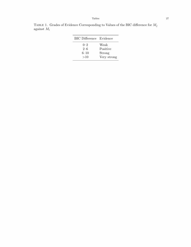
Tables 27
Table 1. Grades of Evidence Corresponding to Values of the BIC difference for Mj
against Mi
BIC Difference Evidence
0–2 Weak2–6 Positive6–10 Strong>10 Very strong
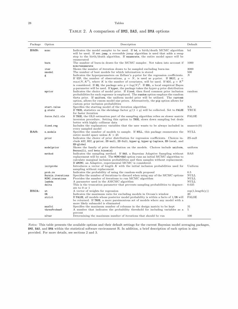
28 Tables
Table 2. A comparison of BMS, BAS, and BMA options
Package Option Description Default
BMS: mcmc Indicates the model sampler to be used. If bd, a birth/death MCMC algorithmwill be used. If rev.jump, a reversible jump algorithm is used that adds a swapstep to the birth/death algorithm. If enumerate, the entire model space will beenumerated
bd
burn The number of burn-in draws for the MCMC sampler. Not taken into account ifmcmc=enumerate
1000
iter Shows the number of iteration draws to be sampled excluding burn-ins 3000nmodel The number of best models for which information is stored 500g Indicates the hyperparameters on Zellner’s g-prior for the regression coefficients.
If UIP, the number of observations, g = N , is used as g-prior. If BRIC, g =max(N,K2), where K is the number of covariates, will be used. If RIC, g = K2
is considered. If HQ, the package sets g = log(N)3. If EBL, a local empirical Bayesg-parameter will be used. If hyper, the package takes the hyper-g prior distribution
N
mprior Indicates the choice of model prior. If fixed, then fixed common prior inclusionprobabilities for each regressor is employed. The random option employs the randomtheta prior. If uniform, the uniform model prior will be utilized. The customkoption, allows for cusom model size priors. Alternatively, the pip option allows forcustom prior inclusion probabilities
random
start.value Specifies the starting model of the iteration algorithm NAg.stats If TRUE, statistics on the shrinkage factor g/(1 + g) will be collected. Set to FALSE
for faster iterationTRUE
force.full.ols If TRUE, the OLS estimation part of the sampling algorithm relies on slower matrixinversion procedure. Setting this option to TRUE, slows down sampling but dealsbetter with highly collinear data
FALSE
fixed.reg Includes the explanatory variables that the user wants to be always included inevery sampled model
numeric(0)
BAS: n.models Specifies the number of models to sample. If NULL, this package enumerates theentire model space unless K > 25
NULL
prior Indicates the choice of prior distribution for regression coefficients. Choices in-clude AIC, BIC, g-prior, ZS-null, ZS-full, hyper-g, hyper-g-laplace, EB-local, andEB-global
ZS-null
modelprior Shows the family of prior distribution on the models. Choices include uniform,Bernoulli, and beta.binomial
uniform
method Indicates the sampling method. If BAS, a Bayesian Adaptive Sampling withoutreplacement will be used. The MCMC+BAS option runs an initial MCMC algorithm tocalculate marginal inclusion probabilities and then samples without replacement.If AMCMC, an Adaptive, experimental MCMC is considered.
BAS
initprobs Introduces a vector of length K with the initial inclusion probabilities used forsampling without replacement
Uniform
prob.rw Indicates the probability of using the random-walk proposal 0.5Burnin.iterations Specifies the number of iterations to discard when using any of the MCMC options NULLMCMC.iterations Provides the number of iterations to run MCMC algorithm NULLlambda A parameter used in the AMCMC algorithm NULLdelta This is the truncation parameter that prevents sampling probabilities to degener-
ate to 0 or 10.025
BMA: wt A vector of weights for regression rep(1,length(y))OR Indicates the maximum ratio for excluding models in Occam’s window 20strict If FALSE, all models whose posterior model probability is within a facto of 1/OR will
be returned. If TRUE, a more parsimonious set of models where any model with amore likely submodel is eliminated
FALSE
maxCol Specifies the maximum number of columns in the design matrix to be kept 31thresProbne0 A number that indicates the probability threshold for including variables as a
percent5
nIter Determining the maximum number of iterations that should be run 100
Notes: This table presents the available options and their default settings for the current Bayesian model averaging packages,BMS, BAS, and BMA within the statistical software environment R. In addition, a brief description of each option is alsoprovided. For more details, see sections 2 and 3.
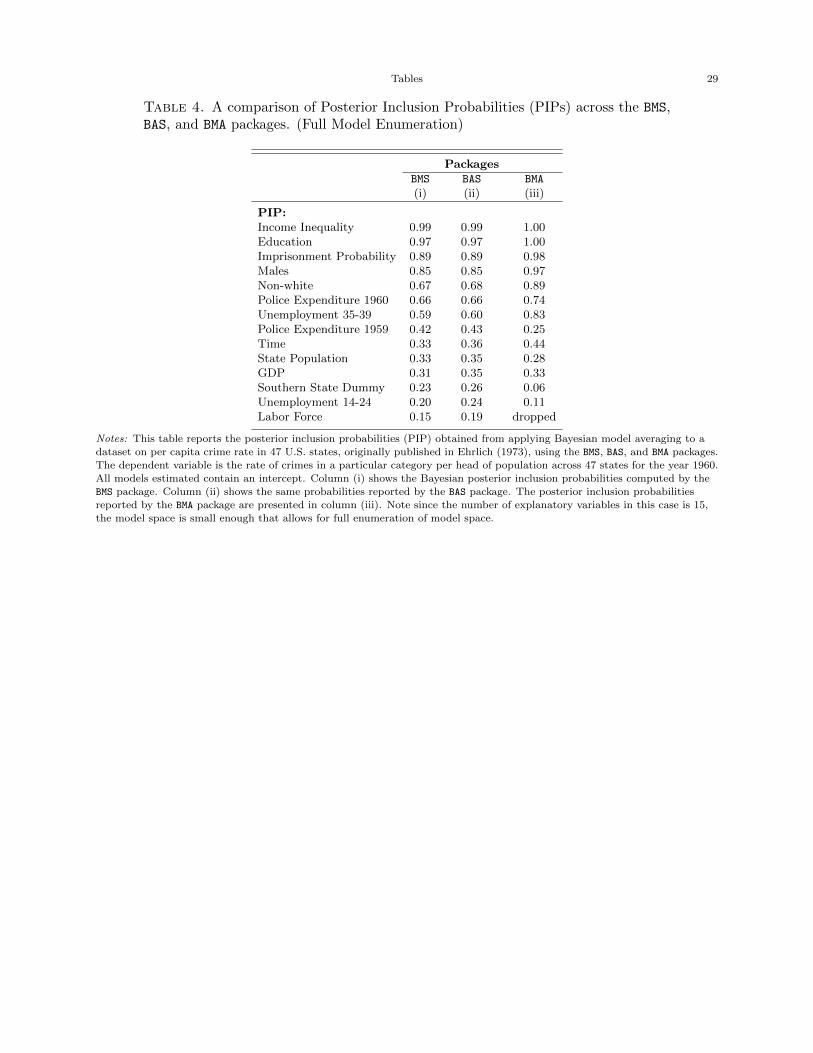
Tables 29
Table 4. A comparison of Posterior Inclusion Probabilities (PIPs) across the BMS,BAS, and BMA packages. (Full Model Enumeration)
PackagesBMS BAS BMA
(i) (ii) (iii)
PIP:Income Inequality 0.99 0.99 1.00Education 0.97 0.97 1.00Imprisonment Probability 0.89 0.89 0.98Males 0.85 0.85 0.97Non-white 0.67 0.68 0.89Police Expenditure 1960 0.66 0.66 0.74Unemployment 35-39 0.59 0.60 0.83Police Expenditure 1959 0.42 0.43 0.25Time 0.33 0.36 0.44State Population 0.33 0.35 0.28GDP 0.31 0.35 0.33Southern State Dummy 0.23 0.26 0.06Unemployment 14-24 0.20 0.24 0.11Labor Force 0.15 0.19 dropped
Notes: This table reports the posterior inclusion probabilities (PIP) obtained from applying Bayesian model averaging to adataset on per capita crime rate in 47 U.S. states, originally published in Ehrlich (1973), using the BMS, BAS, and BMA packages.
The dependent variable is the rate of crimes in a particular category per head of population across 47 states for the year 1960.All models estimated contain an intercept. Column (i) shows the Bayesian posterior inclusion probabilities computed by the
BMS package. Column (ii) shows the same probabilities reported by the BAS package. The posterior inclusion probabilities
reported by the BMA package are presented in column (iii). Note since the number of explanatory variables in this case is 15,the model space is small enough that allows for full enumeration of model space.
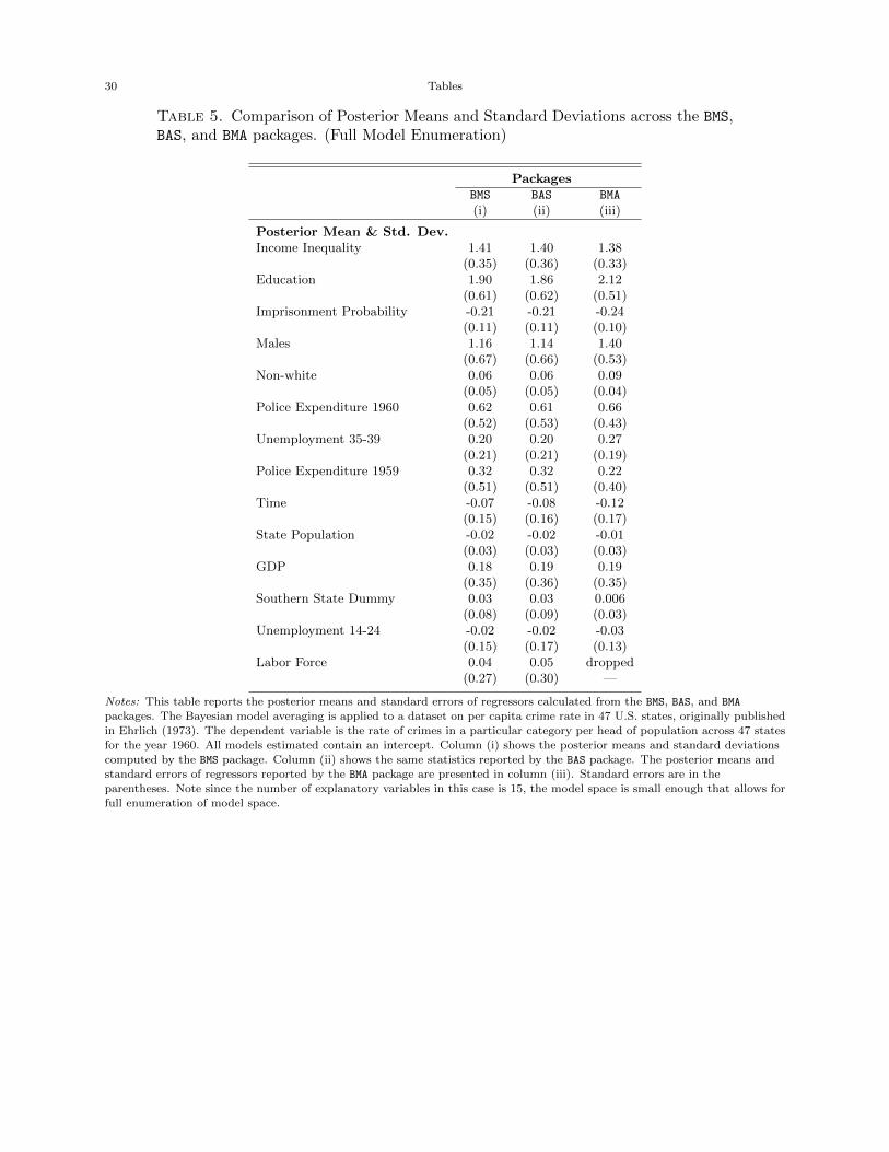
30 Tables
Table 5. Comparison of Posterior Means and Standard Deviations across the BMS,BAS, and BMA packages. (Full Model Enumeration)
PackagesBMS BAS BMA
(i) (ii) (iii)
Posterior Mean & Std. Dev.Income Inequality 1.41 1.40 1.38
(0.35) (0.36) (0.33)Education 1.90 1.86 2.12
(0.61) (0.62) (0.51)Imprisonment Probability -0.21 -0.21 -0.24
(0.11) (0.11) (0.10)Males 1.16 1.14 1.40
(0.67) (0.66) (0.53)Non-white 0.06 0.06 0.09
(0.05) (0.05) (0.04)Police Expenditure 1960 0.62 0.61 0.66
(0.52) (0.53) (0.43)Unemployment 35-39 0.20 0.20 0.27
(0.21) (0.21) (0.19)Police Expenditure 1959 0.32 0.32 0.22
(0.51) (0.51) (0.40)Time -0.07 -0.08 -0.12
(0.15) (0.16) (0.17)State Population -0.02 -0.02 -0.01
(0.03) (0.03) (0.03)GDP 0.18 0.19 0.19
(0.35) (0.36) (0.35)Southern State Dummy 0.03 0.03 0.006
(0.08) (0.09) (0.03)Unemployment 14-24 -0.02 -0.02 -0.03
(0.15) (0.17) (0.13)Labor Force 0.04 0.05 dropped
(0.27) (0.30) —
Notes: This table reports the posterior means and standard errors of regressors calculated from the BMS, BAS, and BMA
packages. The Bayesian model averaging is applied to a dataset on per capita crime rate in 47 U.S. states, originally published
in Ehrlich (1973). The dependent variable is the rate of crimes in a particular category per head of population across 47 statesfor the year 1960. All models estimated contain an intercept. Column (i) shows the posterior means and standard deviations
computed by the BMS package. Column (ii) shows the same statistics reported by the BAS package. The posterior means and
standard errors of regressors reported by the BMA package are presented in column (iii). Standard errors are in theparentheses. Note since the number of explanatory variables in this case is 15, the model space is small enough that allows for
full enumeration of model space.
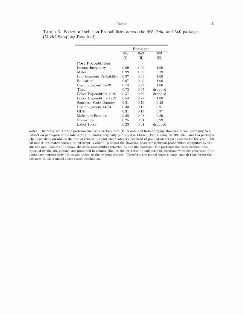
Tables 31
Table 6. Posterior Inclusion Probabilities across the BMS, BMA, and BAS packages.(Model Sampling Required)
PackagesBMS BAS BMA
(i) (ii) (iii)
Post Probabilities:Income Inequality 0.99 1.00 1.00Males 0.99 1.00 0.19Imprisonment Probability 0.97 0.99 1.00Education 0.97 0.99 1.00Unemployment 35-39 0.74 0.93 1.00Time 0.73 0.97 droppedPolice Expenditure 1960 0.57 0.89 droppedPolice Expenditure 1959 0.54 0.22 1.00Southern State Dummy 0.51 0.79 0.42Unemployment 14-24 0.33 0.12 0.91GDP 0.31 0.17 0.97Males per Females 0.25 0.08 0.86Non-white 0.25 0.04 0.99Labor Force 0.23 0.04 dropped
Notes: This table reports the posterior inclusion probabilities (PIP) obtained from applying Bayesian model averaging to a
dataset on per capita crime rate in 47 U.S. states, originally published in Ehrlich (1973), using the BMS, BAS, and BMA packages.
The dependent variable is the rate of crimes in a particular category per head of population across 47 states for the year 1960.All models estimated contain an intercept. Column (i) shows the Bayesian posterior inclusion probabilities computed by the
BMS package. Column (ii) shows the same probabilities reported by the BAS package. The posterior inclusion probabilities
reported by the BMA package are presented in column (iii). In this exercise, 35 independent, fictitious variables generated froma standard-normal distribution are added to the original dataset. Therefore, the model space is large enough that forces the
packages to use a model space search mechanism.
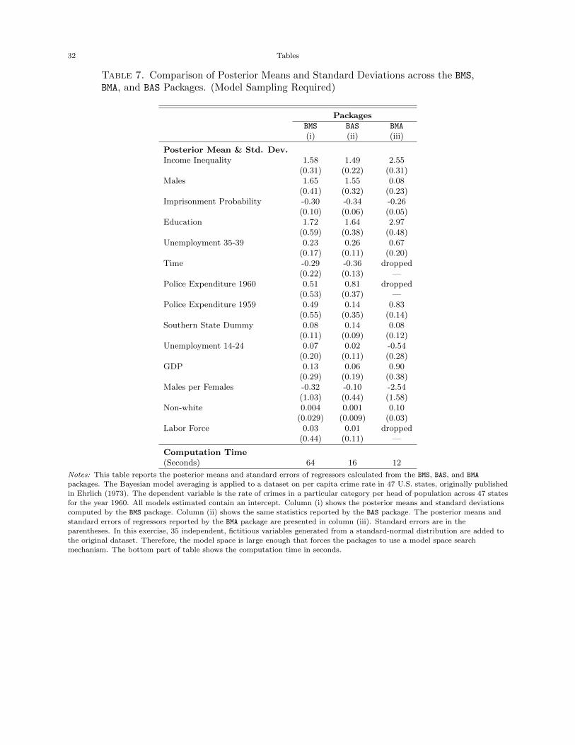
32 Tables
Table 7. Comparison of Posterior Means and Standard Deviations across the BMS,BMA, and BAS Packages. (Model Sampling Required)
PackagesBMS BAS BMA
(i) (ii) (iii)
Posterior Mean & Std. Dev.Income Inequality 1.58 1.49 2.55
(0.31) (0.22) (0.31)Males 1.65 1.55 0.08
(0.41) (0.32) (0.23)Imprisonment Probability -0.30 -0.34 -0.26
(0.10) (0.06) (0.05)Education 1.72 1.64 2.97
(0.59) (0.38) (0.48)Unemployment 35-39 0.23 0.26 0.67
(0.17) (0.11) (0.20)Time -0.29 -0.36 dropped
(0.22) (0.13) —Police Expenditure 1960 0.51 0.81 dropped
(0.53) (0.37) —Police Expenditure 1959 0.49 0.14 0.83
(0.55) (0.35) (0.14)Southern State Dummy 0.08 0.14 0.08
(0.11) (0.09) (0.12)Unemployment 14-24 0.07 0.02 -0.54
(0.20) (0.11) (0.28)GDP 0.13 0.06 0.90
(0.29) (0.19) (0.38)Males per Females -0.32 -0.10 -2.54
(1.03) (0.44) (1.58)Non-white 0.004 0.001 0.10
(0.029) (0.009) (0.03)Labor Force 0.03 0.01 dropped
(0.44) (0.11) —
Computation Time(Seconds) 64 16 12
Notes: This table reports the posterior means and standard errors of regressors calculated from the BMS, BAS, and BMA
packages. The Bayesian model averaging is applied to a dataset on per capita crime rate in 47 U.S. states, originally published
in Ehrlich (1973). The dependent variable is the rate of crimes in a particular category per head of population across 47 states
for the year 1960. All models estimated contain an intercept. Column (i) shows the posterior means and standard deviationscomputed by the BMS package. Column (ii) shows the same statistics reported by the BAS package. The posterior means and
standard errors of regressors reported by the BMA package are presented in column (iii). Standard errors are in the
parentheses. In this exercise, 35 independent, fictitious variables generated from a standard-normal distribution are added tothe original dataset. Therefore, the model space is large enough that forces the packages to use a model space search
mechanism. The bottom part of table shows the computation time in seconds.
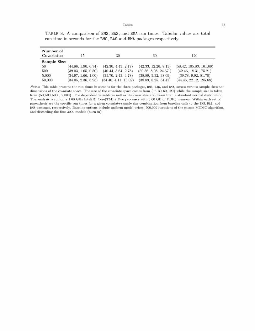
Tables 33
Table 8. A comparison of BMS, BAS, and BMA run times. Tabular values are totalrun time in seconds for the BMS, BAS and BMA packages respectively.
Number ofCovariates: 15 30 60 120
Sample Size:50 (44.86, 1.90, 0.74) (42.30, 4.43, 2.17) (42.33, 12.26, 8.15) (58.42, 105.83, 101.69)500 (39.03, 1.65, 0.50) (40.44, 3.64, 2.78) (39.36, 8.08, 24.67 ) (42.46, 18.31, 75.21)5,000 (34.97, 1.66, 1.00) (35.70, 2.43, 4.78) (38.89, 5.32, 38.09) (39.78, 9.92, 81.70)50,000 (34.05, 2.36, 6.95) (34.40, 4.11, 13.02) (38.89, 8.25, 34.47) (44.45, 22.12, 195.68)
Notes: This table presents the run times in seconds for the three packages, BMS, BAS, and BMA, across various sample sizes anddimensions of the covariate space. The size of the covariate space comes from {15, 30, 60, 120} while the sample size is taken
from {50, 500, 5000, 50000}. The dependent variable as well as the covariates are drawn from a standard normal distribution.
The analysis is run on a 1.60 GHz Intel(R) Core(TM) 2 Duo processor with 3.00 GB of DDR3 memory. Within each set ofparenthesis are the specific run times for a given covariate-sample size combination from baseline calls to the BMS, BAS, and
BMA packages, respectively. Baseline options include uniform model priors, 500,000 iterations of the chosen MCMC algorithm,
and discarding the first 3000 models (burn-in).
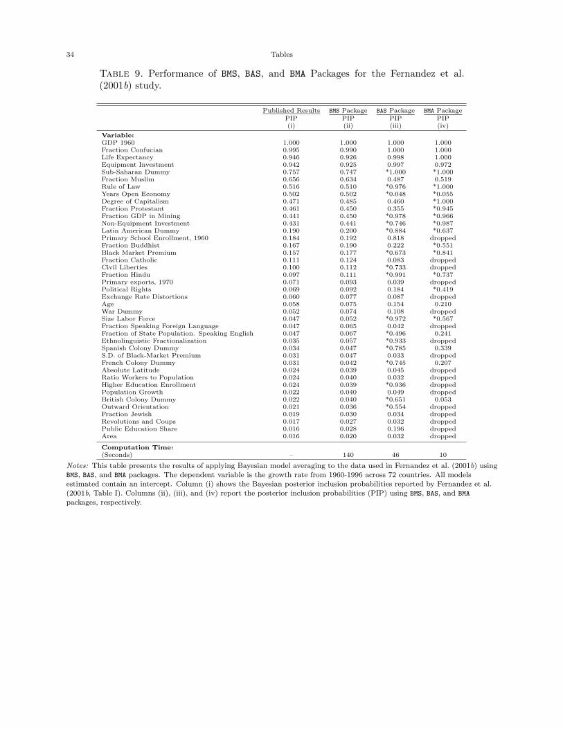
34 Tables
Table 9. Performance of BMS, BAS, and BMA Packages for the Fernandez et al.(2001b) study.
Published Results BMS Package BAS Package BMA PackagePIP PIP PIP PIP(i) (ii) (iii) (iv)
Variable:GDP 1960 1.000 1.000 1.000 1.000Fraction Confucian 0.995 0.990 1.000 1.000Life Expectancy 0.946 0.926 0.998 1.000Equipment Investment 0.942 0.925 0.997 0.972Sub-Saharan Dummy 0.757 0.747 *1.000 *1.000Fraction Muslim 0.656 0.634 0.487 0.519Rule of Law 0.516 0.510 *0.976 *1.000Years Open Economy 0.502 0.502 *0.048 *0.055Degree of Capitalism 0.471 0.485 0.460 *1.000Fraction Protestant 0.461 0.450 0.355 *0.945Fraction GDP in Mining 0.441 0.450 *0.978 *0.966Non-Equipment Investment 0.431 0.441 *0.746 *0.987Latin American Dummy 0.190 0.200 *0.884 *0.637Primary School Enrollment, 1960 0.184 0.192 0.818 droppedFraction Buddhist 0.167 0.190 0.222 *0.551Black Market Premium 0.157 0.177 *0.673 *0.841Fraction Catholic 0.111 0.124 0.083 droppedCivil Liberties 0.100 0.112 *0.733 droppedFraction Hindu 0.097 0.111 *0.991 *0.737Primary exports, 1970 0.071 0.093 0.039 droppedPolitical Rights 0.069 0.092 0.184 *0.419Exchange Rate Distortions 0.060 0.077 0.087 droppedAge 0.058 0.075 0.154 0.210War Dummy 0.052 0.074 0.108 droppedSize Labor Force 0.047 0.052 *0.972 *0.567Fraction Speaking Foreign Language 0.047 0.065 0.042 droppedFraction of State Population. Speaking English 0.047 0.067 *0.496 0.241Ethnolinguistic Fractionalization 0.035 0.057 *0.933 droppedSpanish Colony Dummy 0.034 0.047 *0.785 0.339S.D. of Black-Market Premium 0.031 0.047 0.033 droppedFrench Colony Dummy 0.031 0.042 *0.745 0.207Absolute Latitude 0.024 0.039 0.045 droppedRatio Workers to Population 0.024 0.040 0.032 droppedHigher Education Enrollment 0.024 0.039 *0.936 droppedPopulation Growth 0.022 0.040 0.049 droppedBritish Colony Dummy 0.022 0.040 *0.651 0.053Outward Orientation 0.021 0.036 *0.554 droppedFraction Jewish 0.019 0.030 0.034 droppedRevolutions and Coups 0.017 0.027 0.032 droppedPublic Education Share 0.016 0.028 0.196 droppedArea 0.016 0.020 0.032 dropped
Computation Time:(Seconds) – 140 46 10
Notes: This table presents the results of applying Bayesian model averaging to the data used in Fernandez et al. (2001b) using
BMS, BAS, and BMA packages. The dependent variable is the growth rate from 1960-1996 across 72 countries. All models
estimated contain an intercept. Column (i) shows the Bayesian posterior inclusion probabilities reported by Fernandez et al.(2001b, Table I). Columns (ii), (iii), and (iv) report the posterior inclusion probabilities (PIP) using BMS, BAS, and BMA
packages, respectively.
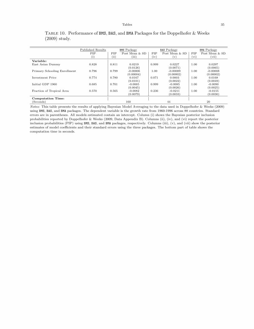
Tables 35
Table 10. Performance of BMS, BAS, and BMA Packages for the Doppelhofer & Weeks(2009) study.
Published Results BMS Package BAS Package BMA PackagePIP PIP Post Mean & SD PIP Post Mean & SD PIP Post Mean & SD(i) (ii) (iii) (iv) (v) (vi) (vii)
Variable:East Asian Dummy 0.828 0.811 0.0219 0.999 0.0227 1.00 0.0297
(0.0126) (0.0071) (0.0065)Primary Schooling Enrollment 0.796 0.799 -0.00006 1.00 -0.00009 1.00 -0.00008
(0.00004) (0.00002) (0.00002)Investment Price 0.774 0.780 0.0167 0.071 0.0003 1.00 0.0168
(0.0101) (0.0022) (0.0049)Initial GDP 1960 0.685 0.701 -0.0065 0.999 -0.0085 1.00 -0.0090
(0.0045) (0.0026) (0.0025)Fraction of Tropical Area 0.570 0.565 -0.0082 0.236 -0.0211 1.00 -0.0155
(0.0079) (0.0033) (0.0030)
Computation Time:(Seconds) 160 44 20
Notes: This table presents the results of applying Bayesian Model Averaging to the data used in Doppelhofer & Weeks (2009)
using BMS, BAS, and BMA packages. The dependent variable is the growth rate from 1960-1996 across 88 countries. Standarderrors are in parentheses. All models estimated contain an intercept. Column (i) shows the Bayesian posterior inclusion
probabilities reported by Doppelhofer & Weeks (2009, Data Appendix B). Columns (ii), (iv), and (vi) report the posterior
inclusion probabilities (PIP) using BMS, BAS, and BMA packages, respectively. Columns (iii), (v), and (vii) show the posteriorestimates of model coefficients and their standard errors using the three packages. The bottom part of table shows the
computation time in seconds.