bayesian model averaging and variable selection in multivariate ... · bayesian model averaging and...

Bayesian Model Averaging and Variable Selection in Multivariate Ecological Models

Ilya A. Lipkovich

Dissertation submitted to the Faculty of the Virginia Polytechnic Institute and State Uni-

versity in partial fulfillment of the requirements for the degree of

Doctor of Philosophy

in Statistics

Eric P. Smith, Chair Keying Ye, Co-Chair

Jeffrey B. Birch Robert V. Foutz

George R. Terrell

April 9, 2002

Blacksburg, Virginia

Keywords: Bayesian Model Averaging, Canonical Correspondence Analysis, Cluster Analysis, Outlier Analysis

Copyright 2002, Ilya A. Lipkovich

Bayesian Model Averaging and Variable Selection in Multivariate Ecological Models

Ilya A. Lipkovich

(ABSTRACT)

Bayesian Model Averaging (BMA) is a new area in modern applied statistics that provides data analysts with an efficient tool for discovering promising models and obtaining esti-mates of their posterior probabilities via Markov chain Monte Carlo (MCMC). These probabilities can be further used as weights for model averaged predictions and estimates of the parameters of interest. As a result, variance components due to model selection are estimated and accounted for, contrary to the practice of conventional data analysis (such as, for example, stepwise model selection). In addition, variable activation probabilities can be obtained for each variable of interest

This dissertation is aimed at connecting BMA and various ramifications of the multivari-ate technique called Reduced-Rank Regression (RRR). In particular, we are concerned with Canonical Correspondence Analysis (CCA) in ecological applications where the data are represented by a site by species abundance matrix with site-specific covariates. Our goal is to incorporate the multivariate techniques, such as Redundancy Analysis and Ca-nonical Correspondence Analysis into the general machinery of BMA, taking into account such complicating phenomena as outliers and clustering of observations within a single data-analysis strategy.

Traditional implementations of model averaging are concerned with selection of variables. We extend the methodology of BMA to selection of subgroups of observations and im-plement several approaches to cluster and outlier analysis in the context of the multivari-ate regression model. The proposed algorithm of cluster analysis can accommodate re-strictions on the resulting partition of observations when some of them form sub-clusters that have to be preserved when larger clusters are formed.

iii

Dedication To the memory of my parents

iv

Acknowledgments

I am grateful to many individuals who contributed to this project, especially to Eric P. Smith and Keying Ye for providing many hours of guidance and stimulating discussions, and for all their patience and encouragement.

Committee members, Jeffrey B. Birch, Robert V. Foutz, and George R. Terrell provided valuable comments and suggestions that helped me to improve the final version of this dissertation.

I would like to thank the U.S. Environmental Protection Agency's Science to Achieve Re-sults (STAR) for Grant No. R82795301 and National Center for Environmental Assess-ment (NCEA) for Grant No. CR827820-01-0 for financial support.

I also want to thank other people who greatly contributed to my former education, in par-ticular my college professor Igor Mandel who first told me about multivariate analysis.

I am grateful to my family who had to put up with me during the last two years.

v

Contents

Introduction .......................................................................................................................1

Chapter 1 Bayesian Model Averaging and Variable Selection .....................................2

1.1 Principles of BMA ........................................................................................2

1.2 Accounting for model selection uncertainty (different views and approaches) ...................................................................................................4

1.2.1 Frequentist view............................................................................................4

1.2.2 Bayesian model averaging ..........................................................................12

1.3 Specifying prior distributions for models and model parameters ...............14

1.3.1 Assigning priors for different models .........................................................14

1.3.2 Assigning priors for the model parameters.................................................16

1.4 Searching for data supported models..........................................................19

1.4.1 Deterministic model search.........................................................................19

1.4.2 Stochastic model search via MCMC...........................................................20

1.4.2.1 Stochastic model search in the model space ...........................................21

1.4.2.2 Stochastic search in the combined model and parameter spaces............22

1.5 Computing Model Posterior Probabilities ..................................................24

1.5.1 Using Bayes Factor approximation.............................................................24

1.5.2 Using MCMC approaches to compute Bayes Factors ................................25

1.5.3 Direct approximation of posterior model probability .................................26

1.6 Inference with BMA. ..................................................................................27

1.6.1 Fully Bayesian model averaging.................................................................27

1.6.2 Semi-Bayesian model averaging.................................................................28

1.6.3 Variable assessment in BMA......................................................................29

1.7 Assessment of BMA performance ..............................................................30

1.8 A simulation study of BMA performance ..................................................31

1.8.1 Out-of-sample performance of BMA..........................................................31

1.8.2 The limits of BMA......................................................................................34

vi

Chapter 2 Implementing BMA for Methods of Multivariate Ordination in Ecological Applications ..............................................................................39

2.1 Correspondence Analysis (CA) ..................................................................39

2.1.2 CA and the reciprocal averaging.................................................................41

2.1.3 CA and the biplot preserving row/column chi-squared distances ..............41

2.1.4 CA and unimodal modeling ........................................................................42

2.1.5 An example of Correspondence Analysis...................................................43

2.2 Relating the latent gradient to the environmental variables........................44

2.2.1 Indirect Multivariate Gradient Analysis .....................................................44

2.2.2 CCA – Multivariate Direct Gradient Analysis............................................44

2.2.3 CCA Example .............................................................................................46

2.2.4 Relationship between CCA and RDA (redundancy analysis) ....................47

2.2.5 Relationship between RDA and Reduced Rank Regression.......................48

2.3 Implementing BMA for RDA and CCA.....................................................50

2.3.1 Computing BIC for the Reduced Rank Regression ....................................51

2.3.1.1 The case of uncorrelated errors with equal variances (CCA and RDA).51

2.3.1.2 The case of unspecified covariance matrix.............................................53

2.3.1.3 The case of diagonal covariance matrix (weighted RDA)......................54

2.3.3 Computing the variance components for CCA and RDA...........................55

2.3.3.1 Obtaining the sampling variance components via bootstrap ..................55

2.3.3.1 Obtaining the variance components due to model selection.................57

2.3.5 Technical details on the algorithm..............................................................58

2.3.6 Applying BMA to a simulated data ............................................................61

2.3.6 BMA analysis for the Great Lakes Data .....................................................65

Chapter 3 Alignment of Eigenvectors when Estimating Variance Components.........72

3.1. Background and motivation........................................................................72

3.2. Theoretical benchmarks ..............................................................................76

3.3. Details on the alignment schemes...............................................................77

3.3.1 Clarkson algorithm......................................................................................77

vii

3.3.2 Procrustes rotation of eigenvectors (PR) ....................................................78

3.3.3 Indirect Procrustes rotation (PRI) ...............................................................79

3.3.4 Rotation Coarsening method (RC)..............................................................79

3.4 The simulation experiment .........................................................................80

3.5 Simulation results........................................................................................84

3.5.1 Comparison of Monte-Carlo estimates of eigenvectors with those obtained by asymptotic formula..................................................................84

3.5.2 Monte-Carlo estimates of the differences between the bootstrap estimates of variance and the theoretical benchmarks................................87

3.6 Comparing the alignment methods on a real data set .................................91

3.7 Aligning eigenvectors in estimation of model selection uncertainty..........96

3.8 Conclusions...............................................................................................100

Chapter 4 Model Based Cluster and Outlier Analysis...............................................102

4.1 Introduction...............................................................................................102

4.2 Model Based Cluster Analysis via MC3 ...................................................103

4.2.1 Existing approaches to Model Based Cluster Analysis ............................103

4.2.2 The basic procedure ..................................................................................104

4.2.3 Extensions for CCA and RDA..................................................................106

4.2.4 Details on the Implementation ..................................................................107

4.2.5 Examples with simulated data ..................................................................110

4.2.6 Classification in the restricted model space..............................................114

4.2.7 An application: analysis of Ohio data.......................................................115

4.2.7.1 Analysis with restrictions at stream level .............................................118

4.2.7.2 Analysis with restrictions at basin level................................................121

4.3 Outlier screening and detection ................................................................125

4.3.1 The MC3 approach ....................................................................................125

4.3.2 Development of BIC.................................................................................126

4.3.3 Implementation .........................................................................................129

4.3.4 Examples with simulated data ..................................................................130

4.3.5 Detecting masking outliers: an example ...................................................132

viii

4.3.6 A simulation study ....................................................................................134

4.4 Conclusions...............................................................................................136

Chapter 5 Extensions and further research ................................................................138

Appendix A Derivation of BIC for RDA .....................................................................140

Appendix B Approximate Equivalence of Alignment by Eigenvectors and by Principal Coordinates................................................................................142

Bibliography ...................................................................................................................143

ix

List of Figures

Figure 1.1 Measuring data overfitting due to model selection...................................35

Figure 2.1 Correspondence Analysis biplot of the hunting spider data .......................44

Figure 2.2 CCA triplot for the hunting spider data ......................................................47

Figure 2.3 Variable activation plot for the simulated data ...........................................63

Figure 2.4 Species and variables biplot enhanced with uncertainty ellipses................64

Figure 2.5 Species and variables biplot enhanced with uncertainty ellipses for the species ...................................................................................................................65

Figure 2.6 Biplot of species and environmental variables using variables selected using CANOCO ............................................................................................66

Figure 2.7 Biplot of sites and environmental variables using variables selected using CANOCO. .........................................................................................................67

Figure 2.8 Variable activation probabilities for variables in BMA..............................68

Figure 2.9 Biplot display of species and environmental variables for BMA analysis 69

Figure 2.10 Plot of species and environmental variables with uncertainty bands for sampling and model uncertainty ...........................................................................70

Figure 2.11 Biplot after scaling variable scores by activation probabilities ..................70

Figure 2.12 Uncertainty intervals for species scores on the first axis............................71

Figure 3.1 Distribution of 1000 bootstrap estimates for the elements of the first 3 eigenvectors (Clarkson method, profile 1)...............................................................88

Figure 3.2 Distribution of 1000 bootstrap estimates for the elements of first 3 eigenvectors (Unaligned eigenvectors, profile 1) .......................................................89

Figure 3.3 Distribution of 1000 bootstrap estimates for the elements of first 3 eigenvectors (Clarkson method, profile 2)..................................................................89

Figure 3.4 Distribution of 1000 bootstrap estimates for the elements of first 3 eigenvectors (Clarkson method, profile 3)..................................................................90

Figure 3.5 Eigenvalues of the FIRO data plotted versus their index numbers.............92

Figure 3.6 Relative discrepancy between bootstrap and asymptotic estimates, l(ej), for the unaligned and aligned eigenvectors .......................................................93

x

Figure 3.7 Relative discrepancy between bootstrap and asymptotic estimates (three methods of alignment versus unaligned eigenvectors).....................................94

Figure 3.8 Scatter diagram of standard error estimates for the elements of the first eigenvector versus their asymptotic benchmarks (unaligned eigenvectors versus aligned eigenvectors) .......................................................................................95

Figure 3.9 Scatter diagram of standard error estimates for the elements of the first eigenvector versus their asymptotic benchmarks (comparing the three methods of alignment) ................................................................................................95

Figure 3.10 Relative discrepancy between bootstrap and asymptotic estimates for different number of retained eigenvectors ..................................................................96

Figure 3.11 Mean absolute deviation of the variance component due to model selection from the benchmark. The two methods of alignment are compared with no alignment .......................................................................................................99

Figure 3.12 Median absolute deviations of model uncertainty standard errors from their benchmarks computed for the first vector of the site coordinates (number of iterations =100) ........................................................................................99

Figure 4.1 Identifying two regression lines defined by partially overlapping clusters ...................................................................................................................111

Figure 4.2 Identifying three clusters defined by their regression lines. The clusters are well separated in the y-direction............................................................112

Figure 4.3 Identifying three clusters defined by their regression lines. The clusters are not separated in the y-direction..............................................................113

Figure 4.4 The algorithm fails to distinguish the two regression lines ......................114

Figure 4.5 Geographical coordinates of steams of the eastern corn belt ecoregion (Ohio). The symbols correspond to different basins ...............................116

Figure 4.6 The biplot diagram for the four largest basins ..........................................118

Figure 4.7 The biplot diagram with the classification results (2 clusters, with restrictions at stream level ). Maximum uncertainty corresponds to p=0.5.............119

Figure 4.8 Geographical coordinates of sites with classification results (2 clusters, restrictions at stream level) .........................................................................121

Figure 4.9 Biplot diagram with classification results obtained with restrictions set at basin level ........................................................................................................122

Figure 4.10 Biplot diagram of t-statistics for individual regressions with the classification results. .................................................................................................124

xi

Figure 4.11 Geographical coordinates of the steams with classification results (3 clusters, restrictions are set at basin level)................................................................125

Figure 4.12 Relationship between p(Mk)/p(M0) and the sample size, nk for β=0.407, n=200.........................................................................................................129

Figure 4.13 Simulated data with variance inflated outliers. p0=0.50, δ1=,∆1=0. The error bars show the probability that an observation is an outlier (multiplied by 5.0). ...................................................................................................................131

Figure 4.14 Simulated data with outliers generated under variance inflation and shift model with p0=0.1 δ1=5. 0, and ∆1=15 ............................................................132

Figure 4.15 Three dimensional scatter plot of the Scottish Hill Racing data. The outliers #7 and #18 mask the outlier #33 ..................................................................133

Figure 4.16 Two dimensional scatter plots with error bars indicating the posterior outlier probability for each observation....................................................................134

Figure 4.17 Mean outlying probabilities for observations added at different distances from the true regression plane in y-direction (the depth of peeling =10 observations)......................................................................................................135

Figure 4.18 Mean outlying probabilities for observations added at different distances from the true regression plane in y-direction (the depth of peeling =50) ...............................................................................................................136

xii

List of Tables

Table 1.1 Summary of approaches that account for model selection uncertainty found in the frequentist literature................................................................................11

Table 1.2 Summary for BMA out-of-sample performance against top, full and true models. Occam’s window=25. The ratios are averages over 200 iterations .......34

Table 1.3 Summary of BMA out-of-sample performance when using different size of Occam’s window (random design and high correlations)...............................34

Table 1.4 Summary of BMA performance against the top, full, and true models when the same data are used for model selection and prediction ...............................36

Table 1.5 Summary of over-performance for BMA, Top model and Full model when predicting the same data that were used for model selection ............................37

Table 1.6 Summary of BMA performance when the same data are used for model selection and prediction for different size of Occam’s window (random design, high correlations)............................................................................................37

Table 2.1 A fragment of the hunting spider abundance data ......................................39

Table 2.2 Coefficients and factor loadings for the simulated rank 2 regression.........61

Table 2.3 BMA output for a simulated example of reduced rank regression .............62

Table 3.1 Profiles of eigenvalues used in the simulation study ..................................84

Table 3.2 Means and standard errors of simulated eigenvectors (Profile 1, using first 3 eigenvectors).....................................................................................................85

Table 3.3 Means and standard errors of the simulated eigenvectors (Profile 2, using first 3 eigenvectors) ...........................................................................................86

Table 3.4 Means and standard errors of the simulated eigenvectors (Profile 3, first 3 eigenvectors).....................................................................................................87

Table 3.5 Absolute difference between bootstrap estimates of standard errors and the asymptotic standard errors .............................................................................91

Table 3.6 Proportion of swaps and sign changes in the first 10 eigenvectors ............94

Table 4.1 The results of cluster analysis with cluster-specific variables: P-values versus posterior effect probabilities...............................................................111

Table 4.2 Group means of the bio-chemical and habitat variables for select basins ...................................................................................................................117

xiii

Table 4.3 The t-scores in basin-specific regressions of IBI on the stressor variables ...................................................................................................................118

Table 4.4 Group means and t-scores from OLS regression for the two clusters. DO, Ph and Zn were log transformed .......................................................................119

Table 4.5 Cross-validation for the two cluster solution ............................................120

Table 4.6 Cross-validation for three cluster solution................................................122

Table 4.7 Summary for individual regression models in 12 basins ..........................123

Table 4.8 Outlier posterior probabilities for the race data. Comparison of two methods ...................................................................................................................134

1

Introduction

Bayesian Model Averaging (BMA) is a new area in modern applied statistics that provides data analysts with an efficient tool for discovering promising models and obtaining esti-mates of their posterior probabilities via Markov chain Monte Carlo (MCMC). These probabilities can be further used as weights for model averaged predictions and estimates of the parameters of interest. As a result, variance components due to model selection are estimated and accounted for, contrary to the practice of conventional data analysis (such as, for example, stepwise model selection). In addition, variable activation probabilities can be obtained for each variable of interest

This dissertation is aimed at connecting BMA and various ramifications of the multivari-ate technique called Reduced-Rank Regression (RRR). In particular, we are concerned with Canonical Correspondence Analysis (CCA) in ecological applications where the data are represented by a site by species abundance matrix with site-specific covariates. Our goal is to incorporate the multivariate techniques, such as Redundancy Analysis, Canoni-cal Correspondence Analysis, etc. into the general machinery of the BMA, taking into ac-count such complicating phenomena as outliers and clustering of observations within a single data-analysis strategy.

The dissertation is organized as follows. The first chapter gives a comprehensive literature review and background on Bayesian Model Averaging. It also contains (Section 1.8) a summary of my simulation study for general evaluation of BMA performance. The second chapter provides a background for the canonical correspondence analysis and related methods in ecological applications and develops the implementation of BMA methodol-ogy for these methods. The third chapter is concerned with a problem of alignment of the singular vectors and associated quantities that arise in all multivariate methods when the variance estimates are obtained by resampling algorithms. We also show its relevance when estimating the variance component due to model selection uncertainty. The chapter introduces a new method of alignment and contains a comparative simulation study. Fourth chapter extends the BMA methodology and stochastic model search onto cluster and outlier analyses. We propose and implement several cluster analysis approaches in the context of the multivariate regression model and extend it to the reduced rank regression context. The models may incorporate restrictions on the cluster solutions when some ob-servations (sites) form sub-clusters which have to be preserved when larger clusters are formed.

Finally we outline possible extensions and research that can be undertaken in future work.

2

Chapter 1 Bayesian Model Averaging and Variable Selection

1.1 Principles of BMA Variable selection has been recognized as “one of the most pervasive model selection problems in statistical applications” (George, 2000), and a lot of different methods emerged during the last 30 years, especially in the context of linear regression (see Miller 1990, McQuarrie & Tsai, 1998, George, 2000). Many researchers focused on developing an appropriate model selection criterion assuming that few reasonable models are avail-able (such as PRESS [Allen, 1971], Mallows’ Cp [Mallows, 1973], Akaike’s AIC [Akaike, 1973], Schwarz’s BIC [Schwarz 1978], RIC of Foster and George [1994], boot-strap model selection [Shao, 1996]). However in reality the researchers often have to choose a single or few best models from the enormous amount of potential models using techniques such as stepwise regression of Efroymson (1960) and its different variations, or, for example, the leaps-and-bounds algorithm of Furnival and Wilson (1974).

Typically researchers use both approaches, first trying to generate several best models for different numbers of variables, and then select the best dimensionality according to one of the criteria listed. Any combination of these approaches to model selection, however, do not seem to take into account the uncertainty associated with model selection and there-fore in practice tend to produce overoptimistic and biased prediction intervals, as will be discussed later. In addition, the statistical validity of various variable selection and elimi-nation techniques (stepwise and forward selection, backward elimination) is suspect. The computations are typically organized in “one variable at a time” fashion seemingly em-ploying the statistical theory of comparing two nested hypotheses, however ignoring the fact that the true null distributions of the widely used “F statistics” (such as F-to-enter) are unknown and can be far from the assumed F distribution (see Miller, 1990).

The two sides of the model selection problem (model search and model selection crite-rion) are naturally integrated in model averaging which overcomes the inherent deficiency of the deterministic model selection by combining (averaging) information on all or a sub-set of models when making estimation, inference, or prediction, instead of using only one model.

In this review we will focus on a standard Bayesian approach to model selection which associates a prior probability with each model M in some model space M (see Key et al., 1999 for differences between the M -close, M -open and M -completed perspectives to modeling) and then uses their posterior probabilities to select one best or “several best” models (for discussion of different approaches to Bayesian model selection see Gelfand

3

and Dey, 1994; Kass and Raftery, 1995). Bayesian Model Averaging (BMA) goes further and uses these probabilities to average the “model parameter” when computing the poste-rior probabilities associated with the other parameters, nested within the model.

BMA is becoming an increasingly popular data analysis tool which allows the data analyst to account for uncertainty associated with the model selection process. In this review, we will try to think about models in a broad context when appropriate since different re-searchers applied BMA within quite different classes of models. In many cases however the model space will be reduced to the subsets of predictors in the linear regression model.

Allowing for a broader class such as the generalized linear model, 1 '( )i i iy g ε−= +x β , where y is linearly related to variables x1,…,xp through a link function g and random error ε with a distribution function f and a variance function v, would expand model space to all possible combinations of subsets of predictors, link and variance functions, and error dis-tributions (see Draper 1995, Raftery 1994). Model context can be expanded in many other directions, for example Hoeting et al. (1996) and Smith and Kohn (1996) consider BMA with simultaneous variable selection and outlier identification. Many applications of BMA are concerned with the model space confined to some special subclass, there are applica-tions of BMA to graphical models (Madigan and Raftery, 1994), regression trees (Chip-man et al., 1998), multivariate regression (Brown and Vannucci, 1998; Noble, 2000), wavelets (Clyde et al., 1998), and survival analysis (Volynsky et al., 1997), just to men-tion a few.

Our research goal centers around multivariate ordination techniques, such as CCA. These methods and the issues of BMA implementation for them will be considered separately in greater detail in Chapter 2 of the dissertation.

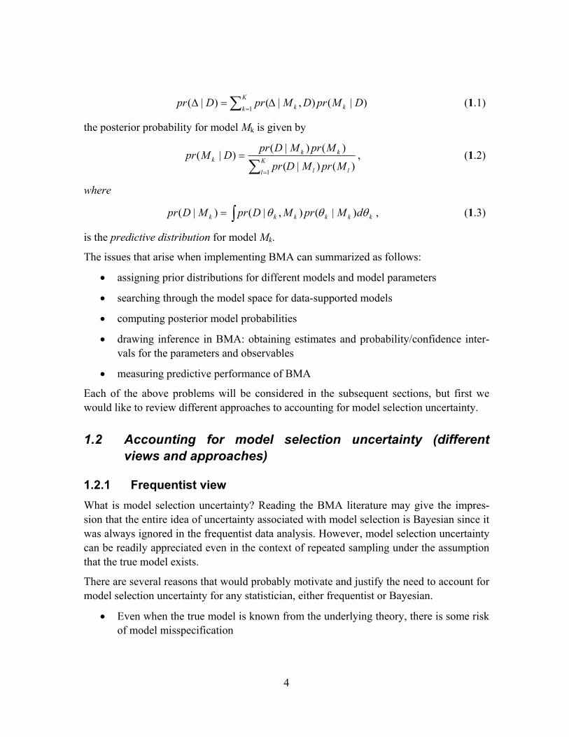
As is clear from the above discussion, BMA arises when the true model is unknown be-fore we look at the data (actually it assumes that there may be no single true model) and it can be viewed as a data analysis tool which in a sense brings together the exploratory phase of the data analysis (model specification) and the confirmatory phase (model esti-mation) by simultaneously searching through data for good models and updating their as-sociated posterior probabilities (if necessary). Then BMA combines the predictions and parameter estimates obtained with different plausible models using their posterior prob-abilities as weights. A popular part of the BMA output is variable assessment which can be done by aggregating posterior weights across only those models where a given variable was present.

More technically, following Madigan and Raftery (1994), if ∆ is the quantity of interest, such as a parameter of the regression model or a future observation, then its posterior dis-tribution given data D and a set of K models is a mixture of posterior distributions (see also Leamer, 1978):

4

)|(),|()|(1

DMprDMprDpr kkK

k∆=∆ ∑ =

(1.1)

the posterior probability for model Mk is given by

)()|(

)()|()|(

1 llK

l

kkk

MprMDprMprMDpr

DMpr∑ =

= , (1.2)

where

∫= kkkkkk dMprMDprMDpr θθθ )|(),|()|( , (1.3)

is the predictive distribution for model Mk.

The issues that arise when implementing BMA can summarized as follows:

• assigning prior distributions for different models and model parameters

• searching through the model space for data-supported models

• computing posterior model probabilities

• drawing inference in BMA: obtaining estimates and probability/confidence inter-vals for the parameters and observables

• measuring predictive performance of BMA

Each of the above problems will be considered in the subsequent sections, but first we would like to review different approaches to accounting for model selection uncertainty.

1.2 Accounting for model selection uncertainty (different views and approaches)

1.2.1 Frequentist view What is model selection uncertainty? Reading the BMA literature may give the impres-sion that the entire idea of uncertainty associated with model selection is Bayesian since it was always ignored in the frequentist data analysis. However, model selection uncertainty can be readily appreciated even in the context of repeated sampling under the assumption that the true model exists.

There are several reasons that would probably motivate and justify the need to account for model selection uncertainty for any statistician, either frequentist or Bayesian.

• Even when the true model is known from the underlying theory, there is some risk of model misspecification

5

• When the true model is not provided by the theory, relying on a single model found by some previous empirical study may result in unstable predictions (due to the fact that the data set used for model search would not capture structural changes that may have occurred after that, or simply because of the inherent sam-pling variation in the training data set)

• Presence of competing models with close predictive performance make choice of the single model arbitrary and dependent upon particular model search procedure

• When estimating the model found by searching the same data set (most typical situation in practice), over-fitting and selection bias occur, which causes the pre-diction intervals to be too narrow and biased

To illustrate these ideas, let us consider model space M generated by all possible subsets of the k predictors in linear regression by adding a multivariate parameter γ=(γ1,.., γk), where a dummy γi is associated with predictor xi (γi =1, when xi is in the model, and γi =0 when xi is not selected). Ignoring for a moment that the exhaustive search of the model space may be infeasible, imagine that we are able to order all the possible models accord-ing to some criterion C, say R2 adjusted, Mallow’s Cp, Akaike’s Information Criterion, or Schwarz’s BIC criterion, and therefore find the best model. A frequentist way of thinking about model selection would be considering it to be an estimation of the true but unknown parameter γ (see for example Shao 1996). Now we can talk about the confidence hyper-cube that will capture possible best models γ* within say a 95% confidence “around” the true γ, which could be obtained if we knew the distribution of test statistic based on maximum of C over the entire model space (see derivation of the distributions for many model selection criteria in McQuarrie & Tsai, 1998.) However, it is still not obvious how the model uncertainty expressed by this “confidence set” of models would further propa-gate into the uncertainty quantified by the prediction interval, and how it can be incorpo-rated when making predictions.

To better understand the source of model selection uncertainty, first observe that the C criterion and its maximum over the model space are random variables. By collecting new data under the same true model and repeating the exhaustive search procedure again, we may end up with a different best model (especially in the presence of competing models), thus obtaining different parameter estimates and hence different predictions. Note that the prediction variability can be partitioned (at least mentally) into three parts

• due to pure prediction error (assuming that the parameters of the true model are known)

• due to variability in parameter estimates fitted under same model (within model variation)

• due to model selection (between model variation).

6

This last part reflects model uncertainty and though it can clearly dominate in the total prediction variability, it is quite surprising that the main concern of statisticians was al-ways centered on the second component dealing with uncertainty due to estimated pa-rameters (Chatfield, 1995). Notice that we can also combine the second and third compo-nents into a single component associated with “parameter uncertainty”, since we can con-sider model selection as a (first) part of parameter estimation. At the model selection stage we simply “estimate” some parameters (coefficients) in the model to be zero. The problem with traditional analysis is of course that the uncertainty associated with this first stage of the estimation procedure is left unaccounted when computing the confidence and prediction intervals based on the selected model.

As we saw, BMA accounts for model selection uncertainty simply by associating a prob-ability with each model and averaging across all or some selected best models using their posterior probabilities when obtaining predictions. By doing so we may bring about an additional variation in prediction which is omitted (erroneously) in the classical data analysis. However, this procedure will also tend to produce more accurate individual pre-dictions. We will see later (section 1.5) how the posterior probabilities can be obtained but now we can assume that, keeping with the frequentist approach for a moment, we could simply use our C criterion to weight different models, when obtaining the estimates and predicted values. This unconditional estimation procedure could be still considered within the realm of classical statistics (see Buckland et al. 1997), as some kind of weighted (or shrinkage) estimator, though the Bayesian interpretation seems to be more natural.

An approach similar to the one outlined above was proposed in Buckland et al. (1997). They consider obtaining model weights by bootstrapping the data set and determining the best model in each bootstrap sample. The model weight now is the proportion of bootstrap samples where it was found best performing. The value of their study however is limited because of the small number of possible models in their examples (up to 10). With a large number of models, we could modify their procedure by performing some deterministic model search in each bootstrap sample. However this bootstrap + search procedure seems awkward in several respects.

• It is not clear how to bootstrap the data, since bootstrapping residuals from the fitted models, for example, would make the data conditional on the fitted model, which is inappropriate for our purposes (some authors suggested using the model with all vari-ables as a basis for bootstrap residuals, see Freedman et al., 1986); on the other hand bootstrapping the original data assumes that predictors are random and may introduce too much noise into the procedure if this is not the case.

• The proposed procedure depends on a particular model search algorithm, and model selection criterion which may not find the model with maximum C, hence bringing about additional uncertainty associated with particular search algorithm.

7

• Retaining only the single best model from the data set seems inefficient even from the frequentist point of view; other reasonable models that fit the same data well could be found during the search and provide valuable information on model selection uncer-tainty (hence we are throwing away exactly what we are trying to generate by boot-strapping the data!)

Therefore it may be more efficient if instead of bootstrapping we find a subset of data-supported models (by employing either deterministic or stochastic search as explained in 1.4.1 and 1.4.2) and use only those with weights determined by C. However, as we will see, this is almost the same as BMA with some appropriate model priors, and when C is taken to be BIC or some other criterion based on penalized likelihood (see Noble, 2000).

One aspect of model uncertainty which however drew a lot of attention among frequen-tists lately is the selection bias inherent in any model estimation preceded by model selec-tion using the same data set (see Miller, 1990; Pötscher, 1991; Breiman, 1992; Chatfield, 1995; Hjorth, 1994; Efron, 2000). The reason why selection bias arises is that the actual population parameters estimated are not those of the true model, but rather those con-strained by all the possible samples that would have produced the model actually selected, given the model selection procedure.

Many researchers reported that the actual P-values computed under the null hypothesis of no effect are by far smaller than their expected values of 0.5, when certain model selection procedures were applied to the data sets generated under the null hypothesis (see the re-sults of a comprehensive simulation performed by Adams, 1991; also see Miller, 1990 and Pötscher, 1991). Note that the model selection bias and over-fitting does not arise if the model search is first performed on a different data set selected independently of the one used for model estimation. Therefore a simple-minded way of avoiding selection bias would be to split the data into two subsets and use one half for model selection and then fit the selected model to the second set. This would be in most of the cases unacceptable, owing to insufficient data. Note, however that the uncertainty due to model selection would still be unaccounted for since the analysis again is based on a single model and repetition of the entire procedure may lead to selecting of a different model (this will be illustrated in sections 1.7 and 1.8).

Several frequentist approaches have been proposed that tried to overcome the over-fitting by incorporating the bias correction mechanism directly into the estimation procedure (see Miller, 1990; Pötscher 1991). For example, Miller (1990) proposed to adjust for the bias in regression coefficients by using conditional likelihood where conditioning occurs on the event that the given selection procedure actually produced the model M. This is equivalent to maximizing likelihood on the reduced space (y,x) by excluding those sam-ples that would not produce the model M. His procedure requires estimation of another parameter, the probability that M is selected by a given search method, and it is accom-

8

plished in a separate Monte Carlo simulation carried out within each iteration of likeli-hood maximization.

However, the prediction intervals obtained with this conditional likelihood would not be much wider than those obtained by the classical procedure (so as to properly account for model selection uncertainty), but only shifted according to bias-corrected parameter esti-mates. This is not surprising since the nature of model uncertainty is broader than just se-lection bias caused by performing model search on the same data.

A different approach was undertaken by Pötscher (1991), who derived the asymptotic dis-tribution for the regression parameter estimates conditional on the event that a particular model has been selected by a given model selection procedure. In particular, he was able to show that the asymptotic distribution of parameter estimators is unaffected by model selection if the model selection procedure is consistent. He warned that the asymptotic distribution can be quite inaccurate in the finite sample case. However, Pötscher (1995) suggested that accounting for model uncertainty can be done by directly incorporating it in the classical estimation procedure, “If the selection process leading to a model M is prop-erly taken into account in the inference procedures, such a ‘non-naïve’ approach will re-sult in correct and not in anti-conservative inference”. However, it seems that conditioning on a single selected model (even if accounting for the selection process), rather than aver-aging over the set of models would always result in over-optimistic prediction intervals.

Efron and Gong (1983) described an interesting example of accounting for the over-fitting by bootstrapping the real data set and carrying out model search and model fitting on each bootstrap sample. Their goal was obtaining a bootstrap estimation of the expected “over-optimism” in the misclassification rate when using the Fisher’s linear discriminant func-tions. The over-optimism R*b for each sample is the difference between the misclassifica-tion rate obtained by applying to the original data (y, X) the prediction rule derived from the bootstrap sample (y*, x*) and the bootstrap estimate of the naïve (apparent) misclassi-fication rate when applying this same rule to (y*, x *). The bootstrap estimate of the ex-pected over-optimism is the average of R*b across the bootstrap distribution. This tech-nique allowed the authors to account for the bias in the prediction errors. However, they did not attempt to improve the prediction by combining models from different bootstrap samples. They observed, however, that the “best variables” varied across samples and none of the variables from the best subset found on the original data set was selected in more than 60% of the bootstrap samples. They commented as follows, “No theory exists for interpreting [this], but the results certainly discourage confidence in the casual nature of the predictors [found on the original set]” (Efron and Gong, p 48).

Freedman et al. (1986) reported the results of a bootstrap simulation experiment with a known true model - simple linear regression. The goal was to obtain less biased estimates of the true MSE (mean squared error), MSPE (mean squared prediction error) and R2 as compared to their naïve over-optimistic counterparts based on the “best” model found by a

9

certain variable screening algorithm. This was accomplished by repeating the entire model search + model fitting procedure on each bootstrap sample and directly estimating the

2**

2 ||ˆˆ||ˆ fullMfull EMSPE ββσ −+= , where the expectation is taken across bootstrap sam-

ples, *ˆMβ are the estimates of parameters for the model M that has been selected in a given

bootstrap sample, and 2ˆ fullσ is the estimate of error variance from the full model estimated on the original data. Unlike Efron and Gong, who bootstrapped the data, the authors used the conditional parametric bootstrap where y*’s were based on adding residuals simulated from 2ˆ(0, )fullN σ to the full model’s fit. The results were found to grossly overestimate the true values. While the bootstrap procedure used may be suspect, it seems that the “true” MSEP approximated by Monte Carlo simulation under the assumption of a known true model may not be the correct target here since it does not account for model uncertainty, while the above bootstrap estimate does. In the light of this maybe the upward biased es-timates reported in Freedman et al. were not so inaccurate.

Breiman (1992) criticized the conditional bootstrap procedure of Freedman et al. and pro-posed a technique which he called “little bootstrap”, essentially a mechanism for produc-ing the bias-corrected Cp statistics via a parametric bootstrap. The new y*’s are generated by adding normal i.i.d. errors to the raw data y (as opposed to the fitted values) with the error variances estimated from the residuals of the full model. The bootstrap samples were then used to produce a sequence of best subset regressions for different number of predic-tor variables and estimate quantities needed for the “bias corrected Cp statistic.” Like Efron and Gong (1983), the author was not clear about interpretation of the model uncer-tainty as manifested in the bootstrap samples. “Or consider the distribution of the esti-mated coefficients: Over many simulated runs of the model, each time generating new random noise, and selecting, say, a subset of size four, the coefficient estimates of a given variable have a point mass at zero, reflecting the probability that the variable has been de-leted. In addition, there is a continuous mass distribution over those times when the vari-able showed up in the final four-variable equation. The relation of this distribution to the original coefficients is obscure.” (Breiman, 1992, p. 751)

Hjorth (1994) considered overcoming selection bias in model selection via cross valida-tion and proposed the CMV (cross model validation) criterion. The key principle was that, “in order to measure model selection effects by validation, model selection errors must be in action during the analysis.” CMV is implemented via the following two-step procedure. In the first step the full model search is performed for each subsample Dj with j-th obser-vation removed, and the sequence of best models Mj(k) among models with k predictors are determined for the range of values of k (note that different samples Dj may produce different sets of best models). Now the best dimensionality k0 is determined by minimiz-ing the cross validation sum of squared residuals, ∑ = −

− −=n

j jj ykynkCMV1

21 ))(ˆ()( with

10

respect to k, where )(ˆ ky j− is a prediction for j-th observation based on sample Dj and model Mj(k). In the second step, the best model is determined by choosing among models with same dimensionality k0 the one with smallest R2. While this procedure helps to ac-count for model selection bias in computing CMV(k), it does not resolve model uncer-tainty in the final selection among the competing models with the same number of vari-ables, k0. A similar approach was proposed earlier in Breiman and Spector (1992). Note the difference between this approach to model selection and the traditional use of cross-validation such as given by the widely used PRESS statistic. While in the latter case (termed partial cross-validation in Breiman & Spector, 1992), the cross-validation statis-tic is simply computed for each prospective model, in the former case (complete cross-validation or cross model validation) model selection is carried out separately for each leave-one-out sample.

Interestingly, in his more recent papers, Breiman has shifted his model selection paradigm from a single-model philosophy toward simultaneously using many models. His “model stacking” and bagging (bootstrap aggregating) estimators (Breiman, 1996; Breiman, 1996a) are essentially model averaging with model weights (shrinking parameters) esti-mated using computationally intensive resampling algorithms. In bagging we (1) use for-ward selection to find the best model for k=1,2,..p. predictors in each bootstrap sample, (2) for each number of predictors, compute averaged predictions and prediction errors across the bootstrap samples (notice that different bootstrap samples may give rise to different selected models for each k). Finally we pick the best among these “averaged models”. Stacking subset regressions also works by combining individual models. First the proce-dure uses a stepwise deletion to find the sequence of best models for k=1,2,..,p predictors in each sample formed by leaving one observation out. Then non-negative model weights are determined by minimizing the following cross-validation sum of squares:

{ }2

1 1ˆ( ) ( ) , ( ) 0n p

i ii ky w k y k w k−= =− ≥∑ ∑ ,

where ˆ ( )iy k− is the predicted value obtained with i-th case left out and using the model with k predictors that was found best in that i-th cross-validation set.

Finally we should mention a recent approach to model selection due to Fan (2001), where estimation of parameters (in the context of wavelet estimation and generalized linear models) is done simultaneously with variable selection. This is accomplished via maxi-mizing the appropriately defined penalized likelihood (instead of the likelihood). The pen-alty function is introduced in such a way that it causes certain coefficients to be estimated as zeros (simultaneously with other non-zero coefficients). Though this approach seems to account for the stochastic error associated with model selection, unlike the BMA ap-proach, it produces only a single model.

11

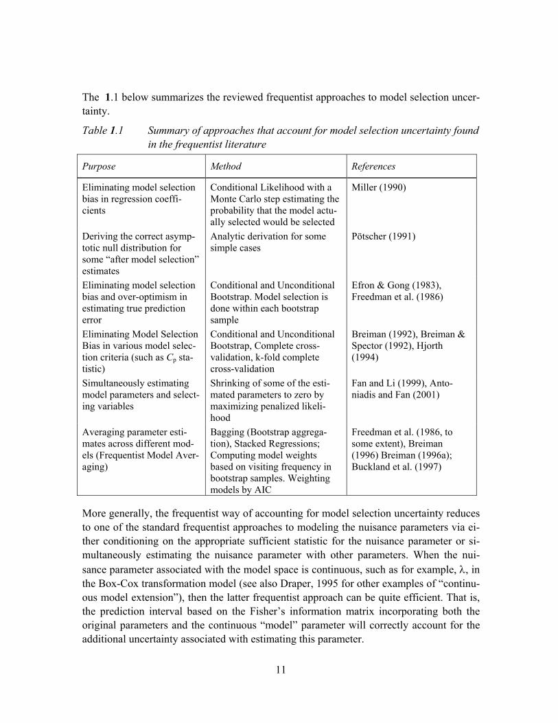
The 1.1 below summarizes the reviewed frequentist approaches to model selection uncer-tainty.

Table 1.1 Summary of approaches that account for model selection uncertainty found in the frequentist literature

Purpose Method References

Eliminating model selection bias in regression coeffi-cients

Conditional Likelihood with a Monte Carlo step estimating the probability that the model actu-ally selected would be selected

Miller (1990)

Deriving the correct asymp-totic null distribution for some “after model selection” estimates

Analytic derivation for some simple cases

Pötscher (1991)

Eliminating model selection bias and over-optimism in estimating true prediction error

Conditional and Unconditional Bootstrap. Model selection is done within each bootstrap sample

Efron & Gong (1983), Freedman et al. (1986)

Eliminating Model Selection Bias in various model selec-tion criteria (such as Cp sta-tistic)

Conditional and Unconditional Bootstrap, Complete cross-validation, k-fold complete cross-validation

Breiman (1992), Breiman & Spector (1992), Hjorth (1994)

Simultaneously estimating model parameters and select-ing variables

Shrinking of some of the esti-mated parameters to zero by maximizing penalized likeli-hood

Fan and Li (1999), Anto-niadis and Fan (2001)

Averaging parameter esti-mates across different mod-els (Frequentist Model Aver-aging)

Bagging (Bootstrap aggrega-tion), Stacked Regressions; Computing model weights based on visiting frequency in bootstrap samples. Weighting models by AIC

Freedman et al. (1986, to some extent), Breiman (1996) Breiman (1996a); Buckland et al. (1997)

More generally, the frequentist way of accounting for model selection uncertainty reduces to one of the standard frequentist approaches to modeling the nuisance parameters via ei-ther conditioning on the appropriate sufficient statistic for the nuisance parameter or si-multaneously estimating the nuisance parameter with other parameters. When the nui-sance parameter associated with the model space is continuous, such as for example, λ, in the Box-Cox transformation model (see also Draper, 1995 for other examples of “continu-ous model extension”), then the latter frequentist approach can be quite efficient. That is, the prediction interval based on the Fisher’s information matrix incorporating both the original parameters and the continuous “model” parameter will correctly account for the additional uncertainty associated with estimating this parameter.

12

However, when the model selection parameter is discrete and multi-dimensional (such as γ), there seems to be no standard frequentist approach to automatically incorporate the un-certainty associated with estimating this nuisance parameter. Conditioning on the model search procedure as in Miller (1990) seems too contrived and underestimates the true model uncertainty. The universal bootstrap approach of Efron and Gong (1983) does not lead to the improved predictions even if it allows one to correct for the prediction bias in terms of the naïve R2. Breiman (1992), Breiman and Spector (1992), and Hjorth (1994) showed how to account for model selection bias when making model selection, which only establishes a more complicated procedure for selecting a single model. After you make the finial selection the same issues of model selection bias arise. The frequentist model averaging approach based on bootstrap weights by Buckland et al. (1997) and the bagging estimators by Breiman (1996a) does not have solid theoretical foundation, it is not clear if their model weights have any attractive properties. As was stressed by Hoeting et al. (1999), the theoretical properties of the model uncertainty assessment via bootstrap are not well-understood.

1.2.2 Bayesian model averaging The standard Bayesian approach to quantifying uncertainty is by incorporating it as an ex-tra layer in the hierarchical model. In BMA we assume an extension of the Bayesian hier-archical model, as explained in George (1999a), “By using individual model prior prob-abilities to describe model uncertainty, the class of models under consideration is replaced by a single large mixture model. Under this mixture model, a single model is drawn from the prior, the prior parameters are then drawn from the corresponding parameters priors and finally the data is drawn from the identified model.”

Within the Bayesian hierarchical mixture framework several different approaches to ac-counting for model selection uncertainty emerged.

Historically, first “occurrence” of Bayesian model averaging can be dated to Leamer (1978), where the expression (1.1) for the posterior mixture distribution was explicitly stated. Then, Mitchell and Beauchamp (1988) in their pioneering work considered an ex-ploratory Bayesian variable selection technique based on a hierarchical model with a “spike and slab” mixture prior for the regression coefficients (that is, a diffuse prior for coefficients included in the model and a mass point at zero for those omitted from the model), which depended on an unspecified parameter φ, defined as a the height of spike divided by the height of the slab. Based on this representation, the posterior model prob-abilities were computed analytically. The analyst was expected to pick the best value of the free parameter φ by looking at the charts with outputs of various quantities, such as P(βi=0|D), posterior expected number of predictors, average predictive error, etc. plotted against φ. Although the final goal was still selecting a single best model, the authors pro-

13

posed using various “model-averaged” quantities such as the variable activation probabili-ties (see section 1.6.3):

∑∈

=≠}:{

)|Pr()|0Pr(ii MjM

ij DMDβ (1.4)

which is now viewed as Bayesian variable assessment (see Meyer and Wilkinson, 1998), and which is also an important part of the BMA output. For data sets with many predic-tors, the authors developed a branch-and-bound method that avoids calculation of sub-models known to have negligible posterior probabilities from previous computations.

George (1986) proposed a minimax shrinkage estimator, which combined regression coef-ficients from different models based on minimum posterior risk.

Draper’s (1995) general approach to accounting for model selection uncertainty was based on the idea of model expansion, i.e. starting with a single good model, M, chosen by the data search, we expand the model space to include models which are suggested by the context, and then average over this class of models. As was noted in Hoeting et al. (1999), Draper however does not address model uncertainty due to selection of variables, which is most important. He distinguishes continuous and discrete model space expansion. Con-tinuous expansion amounts to incorporating an extra hyper-parameter which absorbs the model space and then integrating it out. For instance, instead of considering a single error distribution, we can assume some distribution family indexed by a nuisance parameter α, which has to be integrated out. An example of discrete model expansion would be com-bining estimates from GLM’s with different link functions and error distributions.

George and McCulloch (1993, 1997) elaborated on the original Mitchell and Beauchamp’s (1988) “spike and slab” approach in the context of variable selection in re-gression models. The main crux of their approach was utilizing the Gibbs sampler to si-multaneously move through the space of models and model parameters, which they called Stochastic Search Variable Selection (SSVS). This allowed them to select the “promising subsets” with highest posterior probabilities. Their work was extended by several other researchers. Brown and Vannucci (1998) generalized it for the case of multivariate normal regression, Chipman (1996) developed a framework that allowed for variable selection in the presence of related predictors such as interactions and main effects in designed ex-periments; Geweke (1996) proposed a SSVS methodology similar to that of George and McCulloch (1993) with a different mixture distribution for model parameters represented by a combination of point mass and truncated normal and proposed a more efficient Gibbs sampler. Smith and Kohn (1996) extended the approach of George and McCulloch for the non-parametric spline regression, they applied the Gibbs sampler to selecting the subsets of knots considered as explanatory variables out of some initial set of possible knots. Their approach allowed for simultaneous selection of the transformation for re-sponse variable and weights for the observations.

14

The most universal approach to BMA was developed in the series of papers by Raftery, Madigan, Hoeting, and Volynsky published over the past 5 years. It provides an extremely broad framework allowing for various types of uncertainties in model selection via both deterministic and stochastic search and systematic use of Bayes factors for model com-parison. They developed the methodology that allows the researcher to account for uncer-tainty in such different contexts as:

• variable selection (linear regression and survival analysis)

• choosing among different link and variance functions, and error distributions in GLM

• simultaneous variable and outliers identification (linear regression)

• simultaneous variable selection and variable transformation (linear regression)

Clyde (1999), and Clyde et al. (1996, 1998, 1999) developed several efficient algorithms and approaches for model mixing under orthogonality of predictors. The main idea is that when predictors are orthogonal, averaging across different models is greatly simplified because it can be carried out by sampling in the space of variables rather than models. The approach proved most useful and natural for wavelet estimation (Clyde et al., 1998) and analysis of designed experiments with many factors (Clyde et al., 1996). When the origi-nal predictors are not orthogonal, they can be orthogonalized and same methodology ap-plies, though at the expense of losing somewhat in the interpretation of parameters. How-ever, when the main goal is prediction rather than explanation, this approach becomes ad-vantageous. On the other hand, an emphasis on prediction seems to be instrumental for the BMA philosophy in general.

1.3 Specifying prior distributions for models and model pa-rameters

According to Clyde (1999a), “assigning the prior distributions on both the parameters and model space is perhaps the most difficult aspect of BMA.”

1.3.1 Assigning priors for different models Many authors considered a general variable-specific prior where each variable that is in-cluded in the model has a unique contribution to the prior (Hoeting et al., 1999):

∏=

−−=p

jjji

ijijMpr1

1)1()( γγ ππ , (1.5)

where γij are 0/1 if variable j is absent/present in model Mi. A special case of (1.5) is a size prior (Noble, 2000) where jπ is assumed the same for all variables and as a result, mod-

15

els of equal length receive the same probability: ( ) (1 )k p kipr M π π −= − (k is the number

of variables in Mi). George and McCulloch (1993) suggested using small π so that more parsimonious models would receive larger weight. In the approach proposed in Raftery et al. (1996), π is taken as 0.5 for all variables, which makes all models a priori equally likely.

Philips and Guttman (1998) proposed a separate hierarchical structure for the prior model probabilities, which allows them to (i) give equal probabilities to models with the same number of predictors and (ii) penalize models involving more predictors. The former re-

quirement is satisfied by taking pkkp

kM ,..1,0,)|Pr(1

=

=

−

, where k and p are the number

of selected predictors in model M and the total number of predictors, respectively. To ac-complish the latter requirement, they propose to consider k a Poisson random variate with

the hyperparametes λ and φ, φ

λ+= 1)!(

)Pr(k

kk

. This can be interpreted as if the inclusion of

any variable in the model is equivalent to the occurrence of a rare event, which is often modeled with the Poisson distribution. The authors further motivated the hyperparame-ters’ values as λ =0.5 and φ=0.5. After integrating out k, the prior distribution for model M

becomes 2/1)!(2

)!()Pr(k

kpM k

−= .

Another idea was exploited in Madigan et al. (1995) for elicitation of informative priors in graphical models by collecting imaginary cases from experts and then obtaining model priors as one-iteration updates from the uniform priors with this imaginary data.

Laud and Ibrahim (1996) developed a “fully predictive approach” for prior elicitation similar to that in Madigan et al. (1995). Their updating scheme is more complicated and involves two steps, first priors are updated (analytically) into pr(M|D0) with an imaginary past replicate of the current experiment, D0. At the second step, since D0 is considered as yet-unobserved, they treat pr(M|D0) as a random quantity and finally convert it into an in-formative prior by integrating out D0, now using the expert prediction η as the mean for the imaginary D0. Like in Madigan et al. (1995), they focus on using prior guesses for ob-servables when eliciting priors (such as predicted values η), as opposed to parameters.

Clyde (1999) and George (1999) warned about possible adverse effects of uniform model priors in the presence of multicollinearity. Consider the following example (Clyde, 1999), where we start with a single predictor X1 and assign the prior probabilities of 0.5 to two models ({1}, {1, x1}). Adding a new variable x2, even perfectly correlated with x1 would inflate the probability of 0.5 associated with x1 alone into much larger probability 0.75 distributed over the last three models of ({1},{1, x1}, {1, x2}, {1, x1, x2}), though they clearly represent same x1, now “diluted” with its proxy x2. This inflation in the prior dis-

16

tribution carries over to the posterior distribution and will affect both model selection and model averaging.

All the approaches considered so far treated different components γ as a-priory independ-ent Bernoulli, alternative priors with dependent components were considered in Chipman (1995) and Geweke (1996).

Chipman (1995) developed a method of constructing prior model probabilities so as to satisfy certain constraints imposed by the relationships between predictors, such as hierar-chical interactions, grouped predictors, competing predictors and restrictions on the size of the model. For example, imagine that our variables include factors A, B, C and all their two-way interaction. Then we can require that no two-way interaction is included in the model unless its both main effects (parents) are also included.

1.3.2 Assigning priors for the model parameters The obvious difficulty with assigning priors for the model parameters in BMA is in that using non-informative (improper) priors will result in the improper predictive distributions Pr(D|M) and we cannot interpret them as model probabilities, nor can we interpret their ratios as Bayes Factors which is the key tool in comparing the models (see Gelfand and Dey, 1994, p 503). Therefore many authors proposed various kinds of informative priors. Here we primarily focus on the simple case of normal linear regression.

The research team in Hoeting et al. (1999) proposes assigning priors that are proper but relatively flat over the regions of parameter space where the likelihood is substantial. However they note that highly spread out priors tend to over-penalize larger models. They indicate three approaches:

• “Data-dependent priors” that exert least influence over model selection, used in re-gression and generalized linear models (see Raftery, 1996; Raftery et al., 1997)

• Unit information prior (UIP), a multivariate normal centered at the maximum likeli-hood estimate with variance matrix equal to the inverse of the mean observed Fisher information in one observation. This prior was shown to produce a BIC approximation to the Bayes factors (Kass and Wasserman, 1995). See also Shively et al. (1999).

• Volynsky et al. (1997) proposed combining BMA and ridge regression using a “ridge regression prior” in BMA. This approach is close to the empirical Bayes BMA intro-duced for wavelet estimation in Clyde and George (1999)

The first approach was outlined in Raftery (1996) and Raftery et al. (1997). In Raftery (1996) the case of generalized linear model was considered. The prior for the parameters is selected to be normal for models, say M0 and M1, assuming identity link, normal errors and standardized variables. Transforming variables back to their original units naturally produces normal distribution on the prior β’s which now depends on data through means

17

and variances. The priors on the parameters for a sub-model are derived from the prior on the full model, conditioning on some β’s =0. To arrive at the hyperparameter for the prior distribution, the author uses the Laplace approximation to the Bayes factor, which in-volves β’s and the underlying hyperparameter, and proposes to select ranges for the hy-perparameter so as to make the Bayes factor as stable and close to unity as possible for both nested and non-nested models. This ensures that the prior exerts least influence on the model selection.

Laud and Ibrahim (1995) introduced a “predictive approach to prior specification” in the context of normal linear regression, which utilizes prior guesses of observables such as values of response variable, rather than parameters themselves. The prior means, µm, for β’s under model M and design matrix Xm are derived simply as the OLS estimate based on

η, the prior guesses about the response. That is, ( ) 1' 'm m m m

−=µ X X X η .

Philips and Guttman (1998) proposed eliciting the prior distribution for β in the context of linear regression by splitting the data randomly into two sets and then obtaining the joint posteriors for β and σ by updating their non-informative priors using the first set. At the second step the obtained posterior is treated as prior with the remaining observations. This approach is reminiscent of the Intrinsic Bayes Factors approach of Berger and Peric-chi (1996), and the Fractional Bayes Factors of O’Hagan (1995), however the authors do not seem to recognize it in their paper. See also Gelfand and Dey (1994) for a good dis-cussion of the differences between the Bayes factors, intrinsic Bayes factors, pseudo-Bayes factors, and posterior Bayes factors.

Shively et al. (1999) proposed a general MCMC approach to generate data-dependent pri-ors for non-parametric regression models. Their approach also starts with the non-informative priors and then constructs the UIP priors via the Gibbs sampler. The simula-tion output is further used at the second step of MCMC to sample from the model space. The authors argue that their priors give an approximation to the BIC model selection crite-rion (see section 1.5.1).

George and McCulloch (1993) considered the case of normal linear regression where each component of β is modeled as having come from a mixture of two normal distributions with different variances.

),0(),0()1(~| iiiiii uNvN γγγβ +− (1.6)

(where γi again idicate whether predictor xi is included in the model). Note that the joint distribution of parameters β given γ does not depend on σ and threfore is not of conjugate form. This specification was originally introduced to simplify assigning the hyperparameters v and u, however later the authors seemed to prefer the conjugate form used by many other reserchers (for justification of using non-conjugate priors in variable selection context see Geweke, 1996).

18

Another feature that makes it different from the approaches of most other authors (for example Raftery, 1996; Geweke, 1996) is that instead of putting a single mass point on β=0, in their mixture distribution, they allow it to be continious. This trick was necessary to ensure proper mixing in the multi-parameter Gibbs sampler (see details in next section) so that the corresponding Markov chain is irreversable. However, it turned out that assuming a conjugate prior and integrating out β’s makes this concern quite irrelevant since movement in the Markov chain will occur only in the model space and would not involve β’s at all.

The interpretation of the mixture model (1.6) is as follows: vi should be set small so that if γi =0 the corresponding βi could be safely estimated by 0, ui should be set large so that if γi =1, then the corresponding βi should have a non-zero estimate and included into the model. The authors suggest how to set u and v based on “practical significance”, δ (see George and McCulloch, 1997, p. 344). Imagine that we can set iXY ∆∆= /δ , where ∆Y is the size of the insignificant change in Y, and ∆Xi is the size of the maximum feasible change in Xi. The authors showed how to choose v and u so as to ensure higher posterior weighting for those γ for which |βi|>c when γ=1, where c is a predefined constant. In addition to the variances determined by v and u, the correlation structures can be imposed on the prior distribution of β. The authors suggested data-dependent correlation structure replicating that of the OLS estimates, R ∝ (X′X)-1.

Using a non-conjugate prior results in having no simple analytical expressions for the posterior distribution of γ. As a means to reduce the computational burgen, the same authors proposed a conjugate version of their approach, where

),0(),0()1(~| *2*2iiiiii uNvN σγσγγβ +− (1.7)

As George and McCulloch (1997) noted, the principal advantage of the conjugate hierarchical prior is that it enables analytical margining out of β and σ from γ in the joint distribution p(β,σ,γ|D), thus obtaining the analytical expression for the posterior model probability. The importance of this will be seen in the next section where we will consider the MCMC implementation of the SSVS approach.

Geweke (1996) proposed another approach with non-conjugate priors very similar to that of George and McCulloch. Unlike them, he uses vi = 0, which is equivalent to putting a single mass at βi = 0. That is,

),0()1(~| 0 iiiii uNI γγγβ +− , (1.8)

where I0 is a point mass at βi = 0. Compared to the original approach by George and McCulloch (1993), this corresponds to the practical significance of δ = 0, and as George and McCulloch (1997) pointed out, this criterion will select βi on the basis of how well

19

they can be distinguished from zero rather than their absolute size. This means that any β≠0 will be selected provided a sufficient number of observations.

Summarising the vast literature on assigning priors for the model parameters, we can conclude that the UIP prior which gives rise to the BIC approximation for the Bayes Factors is becoming the most popular, since it allows the researcher to reduce the simulation part of the computations to navigating in the model space, as we will see in 1.4.2.

1.4 Searching for data supported models The topic of selecting the best model has received a considerable attention and generated enormous literature in statistics (see for example Miller, 1990, where selecting subsets in regression is considered). Now it seems that the challenging problem of finding the best subset of variables has somewhat obscured and overshadowed a not less important issue of aggregating many good models even in the idealized situation when the best subsets (with respect to some criterion) can be trivially found. It is interesting to note that many researchers ignored model uncertainty even when the information on model selection un-certainty was a natural byproduct of the proposed methods, such as for example, distribu-tion of different models in multiple runs of stepwise regression with random starting sub-sets (see Miller, 1990), or the output of the leaps and bounds algorithm proposed in Furni-val and Wilson (1974).

Searching for good models is also an integral part of BMA, though it is not obvious from the expression (1.2), which “simply” averages across the complete model space. In most of the cases, especially when different models are generated by subsets of predictors, us-ing (1.2) directly would be infeasible for number of predictors > 25-30 (see George and McCulloch, 1997) due to enormous number of possible models in the summation. There-fore different approaches were proposed for implementing the BMA methodology on a reduced model space. The idea is to search through model space for most reasonable mod-els, that is models supported by the data (Madigan and Raftery, 1994). Two different ap-proaches were proposed in literature, deterministic search and stochastic search on the model space using Markov chain Monte Carlo (MCMC).

1.4.1 Deterministic model search The suggested BMA deterministic search schemes are Occam’s Window method of Madigan and Raftery (1994) and leaps-and-bound technique adopted in Volinsky et al. (1997).

Occam’s Window method is described in Raftery et al. (1994), and Hoeting et al. (1999). The idea is to avoid averaging over the complete space of possible models by restricting it to only the models well-supported by the data. For instance, consider the class

20

≤= CDMpr

DMprMA

i

jji )|(

)|(max:' (1.9)

for some appropriate C, say C=20 (as suggested in Raftery, 1995). This set can be further reduced by eliminating the set B of models that have less posterior support than their own submodels (Occam’s razor).

>⊂∈∃= 1)|()|(

,,':DMprDMpr

MMAMMBi

lilli (1.10)

Then the model averaging is performed over the set A=A’\B.

The approximation provided by this method to full BMA was shown to be good in several applications. Criticism for this approach was expressed by several writers (Clyde, 1999a; George, 1999) that averaging across a relatively small set of models captured by the Oc-cam’s window may result in biased estimates and predictions. The authors of this ap-proach argue that while it certainly overestimates the posterior probabilities of the models it includes, it seems to preserve the ratios of these probabilities (Hoeting et al., 1999, p. 114). Also according to them, there is some philosophical justification for the proposed method as it corresponds to the practice of model rejection well established in the scien-tific community: “models that have been clearly discredited do get discarded in scientific research”. As was argued in Madigan and Raftery (1994), averaging across all models as-sumed in standard Bayesian approach is incorrect, “adopting standard methods of scien-tific investigation, we contest that accounting for the true model uncertainty involves av-eraging over a much smaller set of models” (p. 1536).

Another deterministic way to search for models in A was suggested in Volinsky et al. (1997) and it employs the “leaps and bounds” algorithm adopted from Furnival and Wil-son (1974) and generalized for the non-linear case. It may produce results similar to the Occam’s razor approach, though it apparently lacks the philosophical justification of the latter.

1.4.2 Stochastic model search via MCMC The first applications of the stochastic model search were seen in the Markov Chain Monte Carlo Model Composition, (MC3) in Madigan and York (1995), Clyde et al. (1996), and Stochastic Search Variable Selection via Gibbs sampler of George and McCulloch (1993). The Reversible Jump MCMC algorithm of Green (1995) includes many of these algorithms as special cases (see also Carlin and Chib, 1995).

This universal approach of MCMC became an extremely popular tool in Bayesian compu-tations. Two aspects of MCMC in the context of BMA are that it is

• an excellent search device that allows one to locate good models

21

• a mechanism of computing the posterior probabilities as proportion of visited models

We now consider two different implementations of MCMC in BMA: when the Markov chain is constructed only in the model space and when it is constructed in the combined model and parameters space.

1.4.2.1 Stochastic model search in the model space The MC3 is a special case of the Metropolis-Hastings (MH) algorithm (Hastings, 1970). The main idea of MH algorithm is to set-up an irreducible and aperiodic Markov chain whose equilibrium distribution is the desired posterior distribution (see Smith and Rob-erts, 1993). In the case of model selection, this can be done as follows (Hoeting et al., 1999).

First the Markov chain is constructed, defining a neighborhood nbd(M) for each model. For example, for the linear regression model the neighborhood can be the set of models with either one variable more or one variable less than M, plus the model M itself (Raftery et al., 1997). Define a transition matrix q by setting '( ) 0q M M→ = for )(' MnbdM ∉ and )(',0)'( MnbdMMMq ∈∀≠→ . If the chain is currently in state M, proceed by drawing 'M from transition matrix q. 'M is accepted with probability

=)|()|'(,1min

DMprDMprα (1.11)

Otherwise the chain remains in state M.

Under these conditions, the limiting ratio of the number of times each state (model) is vis-ited to the total number of draws is proportional to the posterior model probability. Note that to be able to compute the ratio, we must know the posterior probabilities pr(M|D) only up to normalizing constant, which can be obtained from the Bayes Factor (BF) as follows. Note that expression (1.11) can be written as

' '( | ) ( )min 1,( | ) ( )

p D M pr Mp D M pr M

α

=

where the ratio '( | ) / ( | )p D M p D M is the Bayes Factor for the two models. Bayes Fac-tors are widely used in Bayesian hypothesis testing as a measure of predictive power for a model M’ against M. In section 1.5.1 we will explain in more detail how to calculate this quantity via various approximations, and in particular will talk about the well known BIC approximation.

One can see that the outlined procedure this is actually a Metropolis algorithm, a special case of the Metropolis-Hasting algorithm, which arises when the proposal probability is

22

symmetric and '( )q M M→ is same as its reverse jump probability, '( )q M M→ . In gen-eral, for the M-H algorithm,

→′′→

=)()|()()|'(,1min

MMqDMprMMqDMprα (1.12)

The information on model posterior probabilities is accumulated while performing the stochastic search. In many cases, however, MC3 can be used just as a searching device, since the posterior probabilities can be obtained via the BIC approximation for Bayes Fac-tors, as shown in section 1.5.1 (see also Noble, 2000), which is in fact a more efficient es-timate. Furthermore, the availability of an analytical approximation for the posterior prob-abilities makes the convergence properties of the underlying Markov chain less relevant (Clyde, 1996; Noble, 2000) and allows for more efficient mixing by restarting the simula-tion at random models and carrying out multiple chains of the MCMC (Noble, 2000; Chipman et al., 1998). Noble (2000) combined the Metropolis algorithm with the Occam’s razor criterion of model screening, which allowed him to reduce the number of candidate models for the final averaging.

As was noted in Clyde (1999a), different versions of this algorithm arise with other choices of proposal probability q(M→ M’), which may lead to procedures that can move more rapidly through the model space. Clyde (1999) uses approximate posterior probabili-ties of variable inclusion for the proposal distribution to target more important variables, rather than proposing all variables to be added or deleted with equal probability 1/p (see also next section)

1.4.2.2 Stochastic search in the combined model and parameter spaces Another MCMC approach was proposed in George and McCulloch (1993). The subset search was implemented via the Gibbs sampler and the movement occurred in the com-bined model and parameter space of the associated Markov chain.

Following George and McCulloch (1993), the Gibbs sampler is used to generate a se-quence γ1, ..., γm, where γ =(γ1,… γp) is a vector of ones and zeros corresponding to the presense/absence of a given variable in the model. This sequence converges rapidly in dis-tribution to pr(γ|D) (that is pr(M|D) in our more general notation) and with high probabil-ity contains most interesting subsets. Those γ with highest probability will appear most frequently and hence will be easier to identify. Furthermore, for the non-conjugate mix-ture prior, the sequence of models is embedded into the auxiliary Gibbs sequence, which is an ergodic Markov chain:

β0, σ0, γ0, β1, σ1, γ1, ..., βj, σj, γj,...,

23

β0, σ0 are initialized to be the least squares estimates of model Y|β, σ2 ~ N(Xβ,σ2I) and γ0 =(1,1,...,1), while the subsequent values βj, σj, γj are obtained by simulating values ac-cording to the following iterated sampling scheme:

),,|(~ 11 −− jjjj Ypr γσββ ),,|(~ 1−jjjj Dpr γβσσ

),,|(),,,|(~ )()(ji

jjji

ji

jjji

ji prDpr γσβγγσβγγ =

)...,,,...,( 11111)(

−−+−= j

pj

ij

ijj

i γγγγγ

As was already mentioned, the authors have to use a continuous prior instead of mass point at βi =0 in the mixture distributions (1.6) and (1.7), because otherwise their Gibbs sampler would get stuck each time it generates βi =0. To obviate this problem and use the mass point representation similar to (1.8), Geweke (1996) proposed an alternative Gibbs sampler implementation, which jointly draws (βi, γi) one at a time given σ, and the other pairs (βl, γl), l ≠i.

For the conjugate prior (1.7), the Gibbs updating scheme is much simpler and involves only the single sequence γ1, ..., γm, when each γ value can be generated componentwise from the full conditionals γi|γ(i), D for i = 1..p, where γi can be drawn in any fixed or ran-dom order. The generation of components in this sequence can be obtained simply as simulations of Bernoulli draws with probabilities that can be easily computed (see details in George and McCulloch, 1997, p. 353) They also note an interesting fact that for the conjugate prior, their Gibbs sampler is equivalent to a Metropolis algorithm modified as follows. Components of γ are randomly permuted and considered to be added or deleted from the model in turn, rather than selected with equal probability 1/p, with the accep-tance probability given by the ratio,

)|'()|(

)|'(DMprDMpr

DMpr+

=α (1.13)

Since α in (1.13) is always < 1, it makes the jump less probable and hence the algorithm is less efficient than the MC3, however this can be somewhat compensated by the fact that in the Gibbs sampler the components are selected cyclically, which ensures better mixing. A hybrid algorithm was considered in Clyde et al. (1996).

Alternatively, Clyde et al. (1996) derived approximate formulas assuming conditional in-dependence of γi‘s, and showed that under orthogonality of predictors (which can be al-ways achieved by an appropriate transformation) MCMC sampling can be replaced by direct importance sampling of the model components elementwise. Clyde and Littman (1998) further developed a sampling-without-replacement algorithm which can be yet an-other efficient alternative to MCMC under orthogonality of predictors.

24

Clyde (1999) also considered the block Gibbs sampler with both γ and σ (when σ is not integrated out) and showed how to implement a very efficient blocked Gibbs sampler, where γ|D, σ2 is distributed exactly as a product of independent Bernoulli distributions and σ2|γ,D has the inverse gamma distribution (again assuming orthogonality of predic-tors). Instead of integrating σ out, the Rao-Blackwellized estimator of marginal pr(γi=1|D) and posterior expectation of model parameters β can be obtained by averaging it over the values of σ2 from the Gibbs sampler.

Clyde (1999) extended this result for generalized linear models by applying the appropri-ate variance-stabilizing transformation and using the approximation for the posterior model probabilities as a product of Bernoulli distributions (see next sections). When the predictors are correlated, Clyde et al. (1996) proposed using orthogonalization of the original model space similar to principal component transformation.

1.5 Computing Model Posterior Probabilities

1.5.1 Using Bayes Factor approximation To compute the posterior probabilities in (1.1) we have to evaluate the marginal likelihood

)|( kMDpr . For certain models such as linear regression with normal errors and conju-gate priors, the expression for the marginal likelihood of model Mk is readily available (see Raftery, 1996; Hoeting et al., 1999). In other cases one can use analytical approxima-tions.

Kass and Wasserman (1995), Kass and Raftery (1995), Raftery (1996) demonstrated vari-ous approximations to (1.3) that can be obtained via the Laplace method. The Bayesian Information Criterion (BIC, Schwarz, 1978) approximation is the simplest.

npMDprMDpr kkkk log)2/(),ˆ|(log)|(log −≈ θ (1.14)

where pk is the number of parameters in the model Mk .

This approximation gives us the expression for Bayes Factor, B10= pr(D|M1)/ pr(D|M0) as

nppB o log)(log2 12

10 −−≈ χ ,

where

)},ˆ|(log),ˆ|({log2 00112 MDprMDprχ θθ −= ,

the standard likelihood ratio test statistic when M0 is nested within M1, p0 and p1, are the number of parameters in M0 and M1.

According to the authors, although this approximation is least accurate and should be of order O(1), (which is not that bad given that the other terms in equation 1.14 go to infinity

25

as n does) however practical experience suggests that it performs surprisingly well, as if it were of order O(n-1/2), see Kass and Wasserman (1995) for justifications. Note that the BIC approximation is indeed of order O(n-1/2) for a certain prior, namely the Unit Informa-tion Prior, described in section 1.3.2, (see derivation in Raftery, 1995, p. 132) and there-fore using BIC though it does not require to specify the priors for the model parameters, implicitly assumes UIP.

Now, if we want to obtain the posterior probabilities by averaging with respect to a se-lected set of K+1 not necessarily nested models, say, we can compare models M1,…Mk to M0 in turn and compute

∑=

=K

rrrkkk BBDMpr

000)|( αα (1.15)

were )()( 0MprMpr kk =α is the prior odds for Mk against M0. (“renormalization of un-normalized posterior probabilities”, Clyde et al., 1996)

Estimating posterior probabilities )|( DMpr k via MC3 or related methods of course would allow us to estimate these probabilities empirically as the proportion of times it was visited during the MC3 simulation, however for computing the acceptance rule in the MC3 algorithm we still need ratios of posterior probabilities for models M1 and M0, say, which can be trivially obtained as 110αB . As was observed in Noble (2000), different forms of the model choice criteria can be translated into the standard BIC approximation by the corresponding adjustment of the prior model probabilities, so that the difference in the cri-teria is absorbed by the α’s. This can be considered yet another way of calibrating the model priors.

1.5.2 Using MCMC approaches to compute Bayes Factors What shall we do if the Laplace approximation to the Bayes Factors does not work? Then we cannot use MC3, which requires the ratio of the posterior model probabilities, however we can resort to other MCMC techniques where the Markov chain is defined on the com-bined space of model and model parameters. The apparent problem is that moving across models with different composition of parameters may render the associated Markov chain not irreducible in the general case. We already saw in 1.4.2 how George and McCulloch (1993) handled it by artificially assigning non-zero priors to the parameters that were sup-posed to be deleted from the model. Carlin and Chib (1995) proposed a general but appar-ently quite wasteful Gibbs sampling scheme by introducing so-called pseudo-priors (or linking densities) that were linking the parameters missing in a given model with that model. The most general approach that allows one to implement the MCMC for the mod-els with variable parameter spaces was introduced in Green (1995) who proposed his Re-versible Markov chain Monte Carlo approach. In general its implementation requires

26

evaluation of the Jacobians associated with transformations from one parameter space to another.

The Monte Carlo estimate for the model probabilities is based on their visiting frequency. Note, however, that when the number of parameters is too large, the MCMC algorithm may present convergence problems and may require special efforts for the problem-specific tuning.

Lewis and Raftery (1997) proposed a combination of MCMC and Laplace approximation for the Bayes factor which they called the Laplace-Metropolis estimator. This method uses the output of Gibbs sampler to estimate the parameters of the M1 and M0 at their pos-terior modes and then plugs it into the expressions for the likelihood and the inverse Hes-sian necessary for the Laplace method.

)~()~|(||)~()~|(||

)|()|(

002/1

0

112/1

1

0

110 θθ

θθprDprprDpr

MDprMDpr

BΨΨ

== ,

where kθ~ and || kΨ are the posterior mode and minus the inverse Hessian of

ln{pr(D|θ)pr(θ)}, evaluated at the posterior mode, respectively.

1.5.3 Direct approximation of posterior model probability Clyde (1999) found that in the case of the normal linear model with orthogonal predictors and known σ (orthogonalization can be accomplished by principal components transfor-mation, also regression with orthogonal predictors becomes of central importance in non-parametric wavelet estimation, see Clyde and George, 1999), the elements of γ are a pos-teriori independent Bernoulli random variables, with probabilities

∏=

−−=p

jjji

ijijDMpr1

1)1()|( γγ ρρ (1.16)

),(1

),(),(

σσ

σρρDO

DOD

j

jjj +

== (1.17)

where ρj is marginal posterior probability and ),( σDO j is the posterior odds for includ-ing variable xj in the model. It was shown in Clyde (1999) how to obtain the exact analyti-cal expression for the posterior odds when the relationship between Y and the predictors is linear. For the non-linear case (such as in GLM), orthogonality of predictors does not lead to posterior independence of the elements of γ. However, ignoring the dependence may lead to reasonable approximations of posterior model probabilities via the approximations of the posterior odds Oj and using it in the equation (1.17) (see Clyde, 1999 for details).

Clyde (1999) also explored an alternative way to approximate the model probabilities via the log-linear representation of the model space. Each model γ can be viewed as a cell in

27

the 2p contingency table that represents model space. Now model probabilities can be rep-resented via the saturated model:

log{ ( | )} ...o j j jk j k jkl j k lj jk jkl

pr Dγ α α γ α γ γ α γ γ γ= + + +∑ ∑ ∑ (1.18)

Note that α0 absorbs the log of the normalization constant. Now, we can estimate the coef-ficients αj for j=1..p, by approximating the expression (1.18) linearly using the representa-tion

eαq += U)log( (1.19)

where elements in vector q are the approximation for the unnormalized model probabili-ties computed for some selected l > p models via the Laplace approximation (as shown in Raftery, 1996). U is an appropriate l X p design matrix that contains the corresponding vectors γ (can be chosen as for the fractional factorial design), and e represents the higher order terms from (1.18) not included in (1.19). Now we can estimate the marginal poste-rior probabilities as

)ˆexp(1)ˆexp(

j

jj α

αρ

+=

where jα are the OLS estimates from (1.19). The posterior model probabilities can be ap-proximated by using (1.16). As Clyde (1991) emphasizes, these model probabilities are mere approximations that will be useful to identify high probability models in the context of importance sampling or as the proposal distribution in the MCMC sampler.

1.6 Inference with BMA. We can distinguish between “fully Bayesian” analysis when both parameters and models are treated in a Bayesian way and semi-Bayesian approach when the estimates of the model parameters are obtained using the classical methods and only the model space is treated in a Bayesian way (Volinsky et al., 1997; Noble, 2000)

How do we use the BMA output to obtain estimates and prediction intervals for the pa-rameters and future observables?

1.6.1 Fully Bayesian model averaging In this case, we either obtain both posterior probabilities and parameter estimates from MCMC (George and McCulloch, 1993), or use the explicit formulae for the posterior dis-tributions of the model parameters, if available (see Raftery et al., 1997, for example). In either case, using MCMC is a standard way of obtaining approximate model posterior probabilities. For the MC3 approach the “model averaged” estimate of a quantity of inter-

28

est can be obtained in general as follows. Let g(Mi) be defined on model space M, then the average

∑ ==

N

ttMg

NG

1))((1ˆ (1.20)

is an estimate of E{g(M)}. ∞→→ N as sa MgEG .))((ˆ , and we can compute a poste-rior mixture distribution (1) by letting ),|()( DMprMg ∆= (Madigan and Raftery, 1994.)

George (1999a) pointed out that when )|( kMDpr can be either computed exactly or ap-proximated very well (using the BIC approximation, for example), we can compute

)|( DMpr k and approximate (1.1) as

)|(),|()|( DMprDMprDpr kkSM k

∆=∆ ∑∈

(1.21)

over the selected subset of models S rather than using the Monte Carlo estimate (14). In the same fashion we can compute, say

)|(),|()|( DMprDMEDE kkSM k

∆=∆ ∑∈

or expectation of any other quantity of interest.

Note that sometimes we can use the ML approximation for the posterior probability, es-sentially providing a link from the fully Bayesian to semi-Bayesian model averaging (Volinsky et al., 1997).

),ˆ,|(),|( DMprDMpr kkk θ∆≈∆

1.6.2 Semi-Bayesian model averaging In the semi-Bayesian approach, it is only the model space that is treated in a Bayesian way. We can still use MCMC or Occam’s window to search for models and use BIC ap-proximation to the Bayes Factors (or some of its generalizations, see Smith and Spiegel-halter, 1980; Noble, 2000) to obtain model weights over the set of the selected models. (Note that the BIC does not require specifying the priors for the model parameters.) Using the model weights, we can aggregate parameter estimates and predictions obtained by applying classical methods to fitting these models.

Averaging parameter estimates across the model space can be interpreted as shrinking es-timates toward zero when the variable is not active in the majority of models. This proce-dure sometimes generates criticism, as to its validity. It seems that combining, say, regres-

29

sion coefficient for the same variable from different models is inappropriate because they are adjusted for different predictors (Draper, 1999) and hence not directly comparable.

Hoeting et al. (1999), although defending the general weighting approach, advises not to abuse it and apply it mostly to observables, such as predicted future observations rather than to the individual coefficients. George and McCulloch (1997) also do not advise to go any further in averaging than combining predictions from different models using posterior model probabilities.

1.6.3 Variable assessment in BMA When BMA is applied to the subset selection problem, its output can be used to rank the variables in order of their importance so as to obtain a single model including the best variables, if needed. This procedure was singled out as Bayesian Variable Assessment (BVA, the term seems to be first used in Meyer and Wilkinson, 1998) and it produces variable activation probabilities (weights), obtained by simply averaging out the posterior model probabilities into a variable weight over the set of models were it is present, as in expression (1.4).

When the predictors are orthogonal, Clyde (1999) and Clyde et al. (1996) showed how to directly obtain the exact or approximate posterior probabilities for variables to be included in the model. These activation probabilities, if known before the model search can be used in MCMC as proposal probabilities.

The posterior effect probabilities prob(β≠0|D) can be compared to the classical P-values. The latter will be biased toward zero because of overfitting. Also P-values cannot distin-guish between the situation when we fail to reject the null hypothesis because of insuffi-cient data and when the data actually provide evidence for H0 (Hoeting et al., 1999). The authors in Hoeting et al. (1999) speculate that their posterior effect probabilities can be associated with scientific significance, as opposed to statistical significance which can sometimes lead to false conclusions.

Finally, we can use variable assessment for building a single model that includes only top variables according to their weights. Such a single model approach would certainly violate the philosophy of BMA, however it can be thought of as one of it possible outputs.

A more subjective interpretation of the model parameters and the associated effect prob-abilities was proposed in Mitchell and Beauchamp (1988), Geweke (1996), Laud and Ibrahim (1995, 1996). In their approach, there is not much physical meaning that can be ascribed to the model parameters, only observable quantities are interpretable. “The linear regression model is a predictive device – its parameters are artificial, not real”, Geweke (1996, p.609). According to Mitchell and Beauchamp (1988), the prior probability prob(βi≠0) represents the proportion of credible experts who would include the variable in the model. The predictive approach to BMA is also inherent in Clyde et al. (1996), since

30

the parameters associated with their orthogonalized predictors clearly do not carry much physical meaning.

1.7 Assessment of BMA performance One of the main arguments for using the BMA is based on its ability to improve our pre-dictions, as measured by the out-of-sample prediction error. Summarizing the experience of several studies, Raftery (1995) made a statement that “in most cases BMA improves predictive performance over the single best model by about the same amount as would be achieved by increasing the sample size by 4%.”

BMA was successfully applied to various statistical methods of data analysis: univariate linear regression (Raftery et al., 1997; George and McCulloch, 1993; Geweke, 1996), multivariate analysis (Brown and Vannucci, 1998; Noble, 2000), survival analysis (Volynsky et al., 1997), generalized linear models (Raftery, 1995; Clyde, 1999), graphi-cal models (Madigan and Raftery, 1994), structural equations (Raftery, 1993), wavelet estimation (Clyde and George, 1999), regression trees (Chipman et al., 1998), and non-parametric regression (Smith and Kohn, 1996; Shively et al., 1999).

An interesting application of BMA methodology in the context of linear regression is a method of simultaneous variable selection and outlier detection presented in Hoeting et al. (1996) and Hoeting et al. (1999a); see also similar development in Smith and Kohn (1996).

In Hoeting et al. (1999) we see several examples of BMA applications, each equipped with a convincing out-of-sample validation in terms of its predictive performance. The cross-validation was performed by splitting each data set into two parts, training set, DT and prediction set, DP. The training set is used for model selection and the second set for prediction. Using several models turned out better than using a single model in most of the cases.

Two measures of predictive ability were used, the coverage for 90% predictive interval, measured by proportion of observation of the second set falling within the 90% of the cor-responding posterior prediction interval (see Hoeting et al., 1999). The second measure is the logarithmic scoring rule of Good (1952). Specifically we measure the predictive abil-ity of a single model M as

{ }∑∈∆

∆−PD

TDMpr ),|(log

And compare it with predictive ability of BMA as measured by

∑ ∑∈∆ =

∆−PD

K

k

Tk

Tk DMprDMpr

1)|(),|(log

31

The smaller the predictive log score for a given model or model average, the better the predictive performance.

An intuitive explanation of such a good performance of BMA was given in George (1999), who noted that BMA-based prediction can be viewed as an application of averaging of several approximately unbiased estimates with weights adaptively account-ing for their varying variance, hence better prediction.

A more analytical argument was used in Madigan and Raftery (1994), which follows from the non-negativity of the Kullback-Leibler information divergence.

{ }[ ] KjDMprEDMprDMprE j

K

kkk ,...,1,),|(log)|(),|(log

1=∆−≤

∆− ∑=

See also Chickering and Heckerman (2000) who used Bayesian networks and found that the predictive ability of model averaging is better than using a single model.

1.8 A simulation study of BMA performance

1.8.1 Out-of-sample performance of BMA To assess the performance of BMA in the case of a multiple linear regression, I carried out a small simulation study using a Visual Basic program that has been developed for a more general multivariate case (see description in Chapter 2). The idea of simulation was to use some “true” model to generate the data and then compare the out-of-sample prediction for the averaged model to that of various candidate models (full model, top selected model, and true model). Of course, the usefulness of the results is limited because the simulation is based on the assumption that a “true” model exists, which may not be the case in a real-life situation. The simulation procedure was as follows:

• Simulate training and prediction data sets under the same generation scheme, DT and DP. The number of explanatory variables was taken to be 20 and the number of cases in both training and prediction data sets was set to 100, and 500. The simulation was carried out for fixed and random X-designs. For the fixed design I used same (gener-ated) values of explanatory variables for both training and prediction data sets; for the random design I generated different X matrices for the two data sets. The design could assume 3 correlation patterns: high (r=0.8), medium (r=0.5) and uncorrelated. For this purpose, variables were divided into 4 groups (x1-x5), (x6-x10), (x11-x15), (x16-x20), with equal correlations within each group. All x’s were standardized to have zero means and unit variances. The values for response variable, y’s, were generated by applying the same coefficients for those variables in the same group, α∈(0.1, 0.2, 0.3, 0.0) and adding normal errors with zero means and unit variances. Notice that the coefficients in the last group are set to zero, which means that the full model is not the true model.

32

To ensure that different data sets are comparable (have similar R2), the α coefficients were adjusted by the appropriate factor, c so as to make the R2 for the simulated data to be 0.5 when the true coefficients are applied. This factor is data-dependent and it is

computed as ( )22011

11/

N

j ijji

c N xα−=

=

= ∑ ∑ , where N is the sample size, α’s are the as-

sumed model coefficients and the x’s are simulated. This can be motivated as follows: for a regression model with random design, unit variance of standard error, and true coefficients, β, the expected R2 is computed as

( ) ( ){ }2 22

1 1/ 1p p

j j j jj jR E x E xα α

= == +∑ ∑%

(see Breiman, 1996), and hence the correction factor needed to achieve a certain target 2tR can be estimated as ( )( )1 2

1 1/ 1N p

t j ij ti jc R N x Rα−

= == −∑ ∑

• Run 20,000 iterations of the MC3 algorithm as described in 1.4.2 on the training data and obtain a list of models and model weights.

• Apply Occam’s window to reduce the model set by dropping the models whose BIC (computed as twice the quantity shown in equation 1.14) are by a certain amount worse than that of the model with highest BIC (see Raftery, 1995, p. 31 for guidelines about interpreting differences in BICs). For this simulation I varied the size of the window from 5 to 25 units of BIC.

• Estimate regression coefficients for the model from the model set using training data (DT). Compute the prediction error measures, based on the differences between actual and fitted values.

Let 21

)ˆ(),( ∑∑ ∈=−=

MjAj

Bij

N

iBiM xyBAPE β , be a measure of prediction error for model

M fitted to data A and applied to predict y’s in data B. This means that the coefficients for a model M are first estimated on data set A and further applied to the explanatory variables in the data B. This quantity can be computed for the top model (model with highest BIC found by our MC3 algorithm), full model and “BMA model”. The fitted vales for “BMA model” are the weighted averages of predictions obtained by using

individual models, ( )ˆ ˆ( | )B Aij jM j M

x P M Dβ∈ ∈∑ ∑M

, where M is the set of active” mod-

els after applying Occam’s razor)

• Compute ),( PTtop DDPE , ),( PT

full DDPE , ),( PTBMA DDPE , and ),( PT

true DDPE as defined above. These quantities are used to compute the relative efficiency of the av-eraged model when applied to the new observations. Of course, we hope that BMA

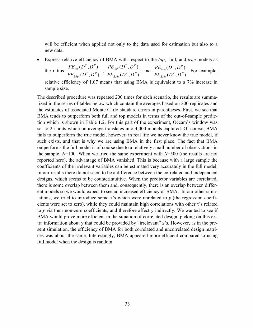
33

will be efficient when applied not only to the data used for estimation but also to a new data.

• Express relative efficiency of BMA with respect to the top, full, and true models as

the ratios ),(),(

PTBMA

PTtop

DDPEDDPE

, ),(),(

PTBMA

PTfull

DDPEDDPE

, and ),(),(

PTBMA

PTtrue

DDPEDDPE

. For example,

relative efficiency of 1.07 means that using BMA is equivalent to a 7% increase in sample size.

The described procedure was repeated 200 times for each scenario, the results are summa-rized in the series of tables below which contain the averages based on 200 replicates and the estimates of associated Monte Carlo standard errors in parentheses. First, we see that BMA tends to outperform both full and top models in terms of the out-of-sample predic-tion which is shown in Table 1.2. For this part of the experiment, Occam’s window was set to 25 units which on average translates into 4,000 models captured. Of course, BMA fails to outperform the true model, however, in real life we never know the true model, if such exists, and that is why we are using BMA in the first place. The fact that BMA outperforms the full model is of course due to a relatively small number of observations in the sample, N=100. When we tried the same experiment with N=500 (the results are not reported here), the advantage of BMA vanished. This is because with a large sample the coefficients of the irrelevant variables can be estimated very accurately in the full model. In our results there do not seem to be a difference between the correlated and independent designs, which seems to be counterintuitive. When the predictor variables are correlated, there is some overlap between them and, consequently, there is an overlap between differ-ent models so we would expect to see an increased efficiency of BMA. In our other simu-lations, we tried to introduce some x’s which were unrelated to y (the regression coeffi-cients were set to zero), while they could maintain high correlations with other x’s related to y via their non-zero coefficients, and therefore affect y indirectly. We wanted to see if BMA would prove more efficient in the situation of correlated design, picking on this ex-tra information about y that could be provided by “irrelevant” x’s. However, as in the pre-sent simulation, the efficiency of BMA for both correlated and uncorrelated design matri-ces was about the same. Interestingly, BMA appeared more efficient compared to using full model when the design is random.

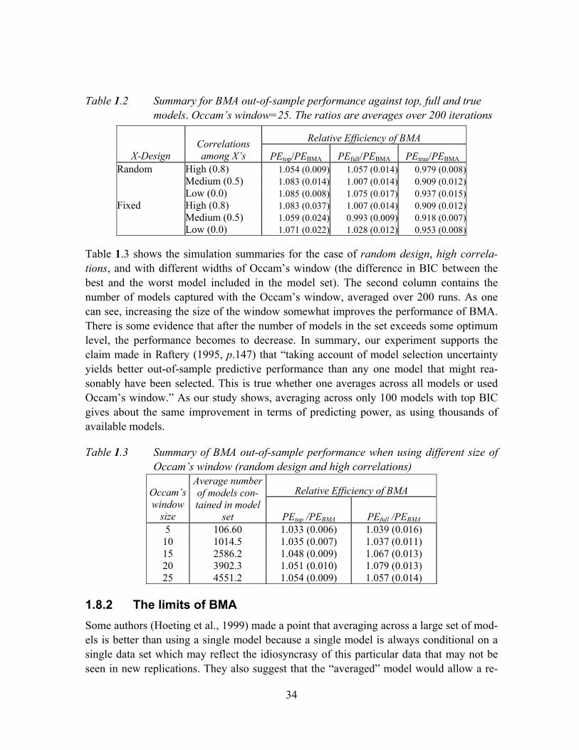
34

Table 1.2 Summary for BMA out-of-sample performance against top, full and true models. Occam’s window=25. The ratios are averages over 200 iterations

Relative Efficiency of BMA

X-Design Correlations among X’s PEtop/PEBMA PEfull/PEBMA PEtrue/PEBMA

Random High (0.8) 1.054 (0.009) 1.057 (0.014) 0.979 (0.008) Medium (0.5) 1.083 (0.014) 1.007 (0.014) 0.909 (0.012) Low (0.0) 1.085 (0.008) 1.075 (0.017) 0.937 (0.015)Fixed High (0.8) 1.083 (0.037) 1.007 (0.014) 0.909 (0.012) Medium (0.5) 1.059 (0.024) 0.993 (0.009) 0.918 (0.007) Low (0.0) 1.071 (0.022) 1.028 (0.012) 0.953 (0.008)

Table 1.3 shows the simulation summaries for the case of random design, high correla-tions, and with different widths of Occam’s window (the difference in BIC between the best and the worst model included in the model set). The second column contains the number of models captured with the Occam’s window, averaged over 200 runs. As one can see, increasing the size of the window somewhat improves the performance of BMA. There is some evidence that after the number of models in the set exceeds some optimum level, the performance becomes to decrease. In summary, our experiment supports the claim made in Raftery (1995, p.147) that “taking account of model selection uncertainty yields better out-of-sample predictive performance than any one model that might rea-sonably have been selected. This is true whether one averages across all models or used Occam’s window.” As our study shows, averaging across only 100 models with top BIC gives about the same improvement in terms of predicting power, as using thousands of available models.

Table 1.3 Summary of BMA out-of-sample performance when using different size of Occam’s window (random design and high correlations)

Relative Efficiency of BMA Occam’s window

size

Average number of models con-tained in model

set PEtop /PEBMA PEfull /PEBMA 5 106.60 1.033 (0.006) 1.039 (0.016)

10 1014.5 1.035 (0.007) 1.037 (0.011) 15 2586.2 1.048 (0.009) 1.067 (0.013) 20 3902.3 1.051 (0.010) 1.079 (0.013) 25 4551.2 1.054 (0.009) 1.057 (0.014)

1.8.2 The limits of BMA Some authors (Hoeting et al., 1999) made a point that averaging across a large set of mod-els is better than using a single model because a single model is always conditional on a single data set which may reflect the idiosyncrasy of this particular data that may not be seen in new replications. They also suggest that the “averaged” model would allow a re-

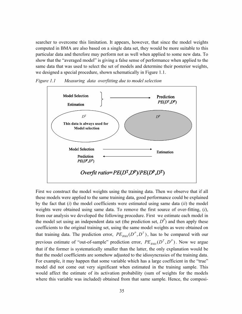
35

searcher to overcome this limitation. It appears, however, that since the model weights computed in BMA are also based on a single data set, they would be more suitable to this particular data and therefore may perform not as well when applied to some new data. To show that the “averaged model” is giving a false sense of performance when applied to the same data that was used to select the set of models and determine their posterior weights, we designed a special procedure, shown schematically in Figure 1.1.

Figure 1.1 Measuring data overfitting due to model selection

Estimation

EstimationPrediction PE(DP,DT)

Model Selection

DT

This data is always used for Model selection

DP

Model Selection

PredictionPE(DT,DP)

Overfit ratio=PE(DT,DP)/PE(DP,DT)

Estimation


Model Selection

DT


DP

Model Selection

PredictionPE(DT,DP)


Estimation


Model Selection

DT


DP

Model Selection

PredictionPE(DT,DP)


First we construct the model weights using the training data. Then we observe that if all these models were applied to the same training data, good performance could be explained by the fact that (i) the model coefficients were estimated using same data (ii) the model weights were obtained using same data. To remove the first source of over-fitting, (i), from our analysis we developed the following procedure. First we estimate each model in the model set using an independent data set (the prediction set, DP) and then apply these coefficients to the original training set, using the same model weights as were obtained on that training data. The prediction error, ),( TP

BMA DDPE , has to be compared with our previous estimate of “out-of-sample” prediction error, ),( PT

BMA DDPE . Now we argue that if the former is systematically smaller than the latter, the only explanation would be that the model coefficients are somehow adjusted to the idiosyncrasies of the training data. For example, it may happen that some variable which has a large coefficient in the “true” model did not come out very significant when estimated in the training sample. This would affect the estimate of its activation probability (sum of weights for the models where this variable was included) obtained from that same sample. Hence, the composi-

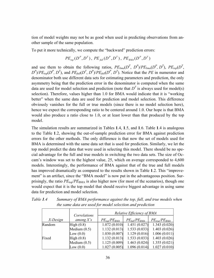
36

tion of model weights may not be as good when used in predicting observations from an-other sample of the same population.

To put it more technically, we compute the “backward” prediction errors:

),( TPtop DDPE , ),( TP

full DDPE , ),( TPBMA DDPE

and use them to obtain the following ratios, PEbma(DT, DP)/PEbma(DP, DT), PEtop(DT, DP)/PEtop(DP, DT), and PEfull(DT, DP)/PEfull(DP, DT). Notice that the PE in numerator and denominator both use different data sets for estimating parameters and prediction, the only asymmetry being that the prediction error in the denominator is computed when the same data are used for model selection and prediction (note that DT is always used for model(s) selection). Therefore, values higher than 1.0 for BMA would indicate that it is “working better” when the same data are used for prediction and model selection. This difference obviously vanishes for the full or true models (since there is no model selection here), hence we expect the corresponding ratio to be centered around 1.0. Our hope is that BMA would also produce a ratio close to 1.0, or at least lower than that produced by the top model.

The simulation results are summarized in Tables 1.4, 1.5, and 1.6. Table 1.4 is analogous to the Table 1.2, showing the out-of-sample prediction error for BMA against prediction errors for the other methods. The only difference is that now the set of models used for BMA is determined with the same data set that is used for prediction. Similarly, we let the top model predict the data that were used in selecting this model. There should be no spe-cial advantage for the full and true models in switching the two data sets. The size of Oc-cam’s window was set to the highest value, 25, which on average corresponded to 4,600 models. Interestingly, the performance of BMA against that of the true and full models has improved dramatically as compared to the results shown in Table 1.2. This “improve-ment” is an artifact, since the “BMA model” is now put in the advantageous position. Sur-prisingly, the ratio PEtop/PEBMA is also higher now (for most of the scenarios), though one would expect that it is the top model that should receive biggest advantage in using same data for prediction and model selection.

Table 1.4 Summary of BMA performance against the top, full, and true models when the same data are used for model selection and prediction

Relative Efficiency of BMA

X-Design Correlations among X’s PEtop/PEBMA PEfull/PEBMA PEtrue/PEBMA

Random High (0.8) 1.072 (0.010) 1.451 (0.027) 1.343 (0.020) Medium (0.5) 1.132 (0.013) 1.533 (0.033) 1.403 (0.026) Low (0.0) 1.030 (0.007) 1.129 (0.016) 1.006 (0.011)Fixed High (0.8) 1.132 (0.013) 1.533 (0.033) 1.403 (0.026) Medium (0.5) 1.125 (0.009) 1.463 (0.024) 1.355 (0.021) Low (0.0) 1.027 (0.005) 1.096 (0.014) 1.027 (0.010)

37

Table 1.5 shows that, as we expected, the ratio for the full model is around unity and the ratio for the model with top BIC is higher when it is applied to the training set. Observe however, that our measure of BMA over-optimism is still rather high, and in most of the cases is even higher than that for the top model. This means that our model weights based on the top BIC that were found in the training data and included in the Occam’s window, may still contain selection bias and probably can be improved by using cross-validation or bootstrap in conjunction with the MC3 approach.

Table 1.5 Summary of over-performance for BMA, Top model and Full model when predicting the same data that were used for model selection

Measure of over-optimism due to selection, Ratio of PE(DT, DP)/PE(DP, DT)

X-Design Correlations among X’s BMA Top Model Full Model True model

Random High (0.8) 1.432 (0.036) 1.394 (0.037) 1.033 (0.024) 1.031 (0.022) Medium (0.5) 1.593 (0.040) 1.512 (0.039) 1.042 (0.028) 1.026 (0.027) Low (0.0) 1.046 (0.026) 1.075 (0.024) 0.969 (0.018) 0.949 (0.020)Fixed High (0.8) 1.593 (0.040) 1.512 (0.039) 1.042 (0.028) 1.026 (0.027) Medium (0.5) 1.513 (0.038) 1.424 (0.037) 1.023 (0.019) 1.024 (0.022) Low (0.0) 1.056 (0.032) 1.083 (0.030) 0.969 (0.021) 0.962 (0.024)

Table 1.6 is analogous to Table 1.3 and it contains simulation summaries of overfitting due to model selection when different sizes of Occam’s window were used (for the case of random design and high correlations). As one can see, increasing the Occam’s window does not remove the part of the over-fitting due to model selection.

Table 1.6 Summary of BMA performance when the same data are used for model selection and prediction for different size of Occam’s window (random design, high correlations)

Measure of over-fitting due to selection bias, Ratio of PE(DT, DP)/PE(DP, DT)

Occam’s window

size

Average number of models in

model set BMA Top Model Full Model 5 106.60 1.415 (0.029) 1.351 (0.027) 1.021 (0.026)

10 1014.5 1.459 (0.033) 1.383 (0.031) 1.049 (0.027)15 2586.2 1.406 (0.032) 1.365 (0.030) 1.033 (0.018)20 3902.3 1.381 (0.025) 1.351 (0.028) 1.020 (0.018)25 4551.2 1.432 (0.036) 1.394 (0.037) 1.033 (0.024)

The rest of the dissertation is organized as follows. In the next chapter we are concerned with implementing BMA for a particular type of multivariate model, Canonical Corre-spondence Analysis (CCA) and some other related multivariate methods which will be introduced accordingly. We develop a comprehensive statistical methodology for using BMA in this class of models: derive an approximation to the BIC criterion, and show how the output of the MC3 procedure can be constructed and analyzed using examples of real and simulated data. Chapter 3 is concerned with an important issue of any multivariate

38

method, which merits a separate study: alignment of eigenvectors in the resampling ex-periments. We propose a general solution and show its efficiency in some simulation ex-periments and using real data as well. Chapter 4 extends the BMA methodology devel-oped for the CCA model to situations when the observational units (sites) are clustered and the relationships between the species and the environmental variables may differ across clusters. Chapter 5 proposes some future research.

39

Chapter 2 Implementing BMA for Methods of Multivariate Ordination in Ecological Applications

This Chapter is concerned with implementation of the BMA methodology that was out-lined in Chapter 1 to a wide class of multivariate methods known as reduced rank regres-sion (RRR). Important members of this class are Canonical Correlation Analysis, Canoni-cal Correspondence Analysis (CCA) and Redundancy Analysis (RDA), which are dealing primarily with ecological data. Our interest in RRR was motivated by these special cases and later we expanded the approach to a broader field of related methods. The plan of the Chapter is as follows. First we introduce Correspondence Analysis (CA) and CCA, and show their connection with other more traditional multivariate methods and with RRR. We also show how the analyses obtained with these methods can be displayed via biplots. Then we implement BMA to RRR and CCA and RDA, as special cases. Finally we pre-sent a real life example of BMA analysis. Some material of this chapter will be published in Case Studies in Bayesian Statistics 6th Workshop (see Lipkovich et al., 2002)

2.1 Correspondence Analysis (CA) Correspondence analysis (CA) is a multivariate technique based on the singular value de-composition (SVD) of an n by m contingency table whose entries are counts or incidences. Throughout this review we will consider the table as representing abundance data that often arise in ecological applications. For this type of data, rows represent sites or other geographical locations and columns represent species, the (i,j)th cell contains the number of species j found at site i. Example: ter Braak considers a study where the data represent counts on 12 species of hunting spider caught in 28 pitfall traps in a Dutch dune area, (ter Braak, 1985). A partial listing of the data is presented in the Table 2.1 below.

Table 2.1 A fragment of the hunting spider abundance data

Site Arct lutePard lugu Zora spin Pard nigr Pard pull AuIo albi Troc terr Alop cunePard montAlop acceAlop fabr Arct peri15 0 2 1 0 0 0 5 0 0 0 0 019 0 3 1 1 0 0 4 1 0 0 0 020 0 3 1 0 0 0 4 1 0 0 0 016 0 2 2 1 0 0 5 1 0 0 0 017 0 1 1 0 0 0 4 0 0 0 0 018 0 2 0 0 0 0 5 1 0 0 0 02 0 1 3 3 6 5 8 1 1 0 0 08 0 7 1 1 1 2 5 3 1 0 0 0

40

In situations when rows and columns are related, CA will help to graphically summarize and represent the data by assigning sets of scores to rows and columns as follows. For a detailed exposition of the method see Greenacre (1984).

First we transform the data as

1/21/2YCRY −−=* , (2.1)

where Y is the n by q contingency table, R and C are the diagonal matrices with the row and column totals, respectively. Applying the SVD results in the decomposition:

'QPΛY =* (2.2)

where P and Q are orthogonal matrices, and Λ is a diagonal matrix of singular values (see Gabriel, 1971; Gower and Hand, 1996). This means that the rectangular matrix Y* can be represented as a linear combination of the matrices defined by the outer products of the columns of P and Q (denoted by p and q, respectively).

∑=

λ=R

rrrr qpY

1

'* (2.3)

From (2.2) it follows that we can also write:

( ) ( ) 'QQΛYY PPΛYY 2*'*'2'** == and (2.4)

This can be also re-written as the eigenvalue problems:

( ) ( ) rrrrrr λandλ qqpp 2*2'== YY YY '*** (2.5)

Expressions (2.4) and (2.5) show that the SVD combines the two separate eigenvalue de-

compositions for the associated squared matrices ( )'** YY and ( ) *YY '* . From (2.2) we can also write:

'*'* ΛQYP PΛQY == and (2.6)

Note that formulas (2.6) express the components of the characteristic vectors pr as linear combinations of qr and vice versa with the data elements yij as weights.

Now, we define the row and column scores (or standard coordinates, [Greenacre, 1984]) PRP 2/1* −= and QCQ 2/1* −= , so that the following defining relations hold

*2**2*'rrrrrr λandλ qqpp == −−−− YRYC YYCR 1'111 (2.7)

Note that P*ΛQ*’ forms a decomposition of the matrix R-1YC-1, since * *' 1/ 2 ' 1/ 2 1/ 2 * 1/ 2− − − −= =P ΛQ R PΛQ C R Y C , and substituting Y* with the expression from

(2.1).

41

There are three different interpretations that can be associated with this decomposition: (i) reciprocal averaging or scaling, (ii) approximation of the chi-squared distances, and (iii) approximation of the unimodal bivariate surface with latent variables, which are consid-ered briefly in the subsequent subsections.

2.1.2 CA and the reciprocal averaging Now using the definitions of P* and Q* and (2.6) we can write the row and column scores as weighted averages of each other

∑∑

=

jij

jrjij

rir y

qypλ

*

* and ∑∑

=

iij

iriij

rjr y

pyq

*

*λ (2.8)

For abundance data, the expressions (2.8) have the following interpretation (see ter Braak, Prentice, 1988; Gower and Hand, 1996). The site-scores are attracted toward species-scores in which they have high frequencies in the relevant row and vice-versa.

The expressions in (2.8) also suggest the following algorithm of finding the row and col-umn scores. Start with some arbitrary scores and then update them using (2.8) until con-vergence, which will give you a pair of row and column scores with the associated singu-lar value. This procedure can be repeated on the reduced data: 'λ 11 qp1−*Y , as follows from the decomposition (2.3). (In what follows Y* is redefined to be the transformed data in this reduced form.) This algorithm results in the well-known power method for finding the first eigenvalues and eigenvectors of a positive semi-definite matrix, here it is applied to *' *Y Y .This method was known and used for ecological ordination for quite a while un-der the name of reciprocal averaging. Typically, it was applied only once to extract the first non-trivial component of the data.

2.1.3 CA and the biplot preserving row/column chi-squared dis-tances

It is quite obvious from (2.8) that there is a trivial solution when λ1 =1 and all the scores are equal to 1. This trivial solution corresponds to the maximal unit eigenvalue of the ma-trix Y* and should be discarded from the analysis. Therefore, we can simplify matters by subtracting the first element R11C11R '' /)( 2/12/1

111 =qpλ (1 is the vector of ones) from Y* as suggested by Equation 2.3. This leads to the following well-known transformation:

ji

jiijij yy

yyyyy

••

••••−=

/* (2.9)

42

where •••• yyy ji ,, are totals for the i-th row, j-th column and the grand total for the abun-

dance matrix, respectively. The quantities *ijy are also called the chi-squared (χ2) contribu-

tions because their squares are proportional to the contribution of the (i,j)-th cell of the n by q table in the Pearson’s χ2 test for the independence between rows and columns. We can now observe that by performing the SVD on the Y* matrix and forming P*Λ, we will be able to represent (approximately) the χ2 distances between the rows (sites) of the origi-nal matrix Y by the Euclidian distances between the rows of the P*Λ. Alternatively, we may represent the χ2 distances between the columns by the Euclidian distances of the rows of Q*Λ. Note that the χ2 distance between rows i and j of the matrix Y is defined as follows

∑=

−=

m

k j

jk

i

ik

kij r

yry

cd

1

2

2 1 ,

where ci and ri denote the respective diagonal elements of the matrices C and R. The χ2 distance between the columns is defined similarly.

This gives rise to a biplot which represents the first two coordinates of the matrices P*Λ and Q* or P* and Q*Λ (see Gabriel, 1971; Gower and Hand, 1996). The classical corre-spondence plot, however uses the first two columns of matrices P*Λ and Q*Λ. To better appreciate, though hardly to remove the confusion that stems from all the different repre-sentations of the CA, refer to the corresponding chapter of Gower and Hand (1996).

2.1.4 CA and unimodal modeling It has been shown that the row and column scores obtained in CA also provide the first-order approximation to the maximum likelihood estimates of the xi and uj scores in the la-tent gradient model, popular in some ecological applications (see ter Braak, 1985; Lynn and McCulloch, 2000).

2

2)(21

j

jijij t

uxa

−−=η (2.10)

where,

ηij is related to the cell’s expected mean µij by a link function (typically log in this type of applications)

xi is a latent fixed effect associated with i-th site.

uj is the optimum or mode of the response curve associated with j-th specie

aj is the maximum of the expected response curve

43

tj is the tolerance that measures the curve width

One should bear in mind that the approximation is valid only when species follow the so-called packing model conditions: abundances have Poisson distribution and the response curves are Gaussian, with homogeneously distributed optima and equal tolerances and maxima (ter Braak, 1985).

The parameterization (2.10) can be interpreted using niche theory as follows: each species occupies a different niche in their habitat which corresponds to the optimal environmental conditions for that species. Therefore, the abundances of the species vary unimodally with respect to some environmental gradient.

2.1.5 An example of Correspondence Analysis This example is borrowed from ter Braak (1986). The data are the counts of 12 species of hunting spiders caught in pitfalls traps in a Dutch dune area (see Table 2.1). The diagram in Figure 2.1 shows the ordination of the species and sites obtained by the correspondence analysis. The computations and the diagram were produced with the Biplot macro pro-grammed by the author (see Lipkovich and Smith, 2001; the macro is available at http://www.stat.vt.edu/facstaff/epsmith.html.) For the interpretation of the diagram, note that species are situated at the centroid of the points for sites in which they occur. There-fore, the points representing the species of spider may indicate the ideal environmental conditions pertinent to the habitat of that specie (their niche). One can see that the data are quite spread out. For instance, Arct peri is plotted closest to sites 26, 24, 27, 22, 23, 28, and these are the only sites where it was found. The centroids actually represent means weighted by the abundances of the specie at the respective sites, therefore on the diagram, the sites close to the specie point tend to have a higher abundance that sites farther away from that specie point.

The distances between the species approximate their dissimilarities as measured by the χ2 distance between the corresponding columns of the original abundance data table. Note, that it captures the difference in relative profiles of species k and l say, rather than differ-ences in absolute counts.

∑=

−=

n

i l

il

k

ik

ikl c

ycy

rd

1

22 1

One can also observe clustering of the sites and species along some imaginary directions, which may correspond to some environmental conditions to be explored later.

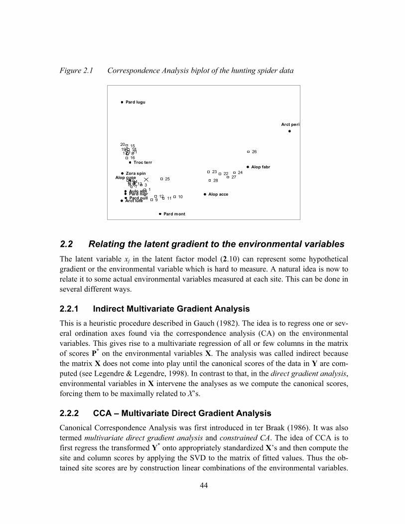
44

Figure 2.1 Correspondence Analysis biplot of the hunting spider data

Arct peri

Alop fabr

Alop acce

Pard mont

Alop cune

Troc terr

AuIo albiPard pullPard nigr

Zora spin

Pard lugu

Arct lute

26

2427

2223

28

1011

25

129

13137

41465

218

2

1817

16

2019

15

2.2 Relating the latent gradient to the environmental variables The latent variable xj in the latent factor model (2.10) can represent some hypothetical gradient or the environmental variable which is hard to measure. A natural idea is now to relate it to some actual environmental variables measured at each site. This can be done in several different ways.

2.2.1 Indirect Multivariate Gradient Analysis This is a heuristic procedure described in Gauch (1982). The idea is to regress one or sev-eral ordination axes found via the correspondence analysis (CA) on the environmental variables. This gives rise to a multivariate regression of all or few columns in the matrix of scores P* on the environmental variables X. The analysis was called indirect because the matrix X does not come into play until the canonical scores of the data in Y are com-puted (see Legendre & Legendre, 1998). In contrast to that, in the direct gradient analysis, environmental variables in X intervene the analyses as we compute the canonical scores, forcing them to be maximally related to X’s.

2.2.2 CCA – Multivariate Direct Gradient Analysis Canonical Correspondence Analysis was first introduced in ter Braak (1986). It was also termed multivariate direct gradient analysis and constrained CA. The idea of CCA is to first regress the transformed Y* onto appropriately standardized X’s and then compute the site and column scores by applying the SVD to the matrix of fitted values. Thus the ob-tained site scores are by construction linear combinations of the environmental variables.

45

The technique allows one to display the site scores, species scores and environmental variables on the same ordination diagram.

When the method was first introduced (ter Braak, 1986), the algorithm was presented that constructed the site scores by interleaving the iterations of reciprocal averaging with the weighted multiple regression of the current site scores on the environmental variables (weighted by the row totals) and replacing the site scores with the fitted values in the sub-sequent iterations. This computationally awkward procedure, though may appeal to the intuition of “simultaneously obtaining the weighted averages and the constrained scores,” somewhat obscures the theoretical features of the method.

The procedure is equivalent to the following (see ter Braak and Verdonschot, 1995; Leg-endre and Legendre, 1998). First we transform the abundance data Y and the environ-mental variables X as

ji

jiijij yy

yyyyy

••

••••−=

/* j

jijij s

xxx

−=* ,

where columns of X are centered and standardized using its mean and standard deviation, weighted by the row totals of the abundance matrix Y: •••= yyw i

ri /)( :

∑=

=R

i

riijj wxx

1

)( ∑=

−=R

i

rijijj wxxs

1

)(2)( ,

where R is the number of rows in Y. Denote Xw=R1/2X*, (that is rows of X* are weighted by the row totals of Y, the elements of the diagonal matrix R). Then we compute ˆ

w=Y X B , where B is the matrix of regression coefficients obtained by applying the mul-tivariate OLS regression to Y* and Xw, and

* * 1 * 1/ 2 * ' 1 ' *( ) ( )w w w− −= =B X 'RX X 'R Y X X X Y

Notice that the described procedure differs from the traditional weighted least squares in that only the X’s are weighted and the fitted values are obtained by applying the regres-sion coefficients to the weighted Xw. Another way of looking at this procedure is writing ˆ

w=Y H Y , where ' 1 '( )w w w w w−=H X X X X is the idempotent projection matrix based on the

standardized and weighted X’s

The SVD is applied to the matrix of fitted values Y to produce ˆ '=Y PΛQ . The output contains the rescaled coordinates for the rows of Y (sites), columns of Y (species), and columns of X (environmental variables). Site coordinates (in the space of Y’s) are given by 1*2/1* −−= QΛYRP . Fitted site coordinates (in the space of X) are given by

PRP 2/1* −=fit . Species coordinates are given by QCQ* 2/1−= . Either P* or *fitP can be

paired with Q* to form a biplot. The commonly used is the GH biplot which emphasizes

46

the distances between species (see Gabriel, 1971) can be obtained by post multiplying Q* by the diagonal matrix of singular values Λ. The JK biplot is constructed by post-multiplying P* by Λ. The coordinates for the environmental variables X can be added on the same diagram to form a triplot using weighted correlations of the (fitted) site coordi-nates and the original X’s. We propose to enhance these graphs with the “error bars”, or ellipses representing uncertainty due to both sampling variability and model selection, ob-tained from the BMA output. BMA output can be also used to construct prediction areas for “new observations” which allows the researcher to evaluate the limits of impact due to possible changes in explanatory variables.

As we already saw, CCA appeared under different names, such as constrained CA, direct gradient analysis, constrained ordination, etc. Now we will show that it is a very close relative to the redundancy analysis (Legendre and Legendre,1998), which arises as a spe-cial case of the so-called reduced rank regression (see ter Braak, 1994; Tso, 1981; Davies and Tso, 1982) and we will discuss it in more detail in section 2.2.4.

2.2.3 CCA Example Continuing with the example from ter Braak (1986), we add some environmental variables measured at each location: Water content- percentage of soil dry mass, Bare Sand – per-centage cover of the moss layer, Fallen Twigs – percentage cover of fallen leaves and twigs, Cover Moss – percentage cover of the moss layer, Cover Herbs – percentage cover of the herb layer, and Light Refl – reflection of the soil surface with cloudless sky. The biplot (actually triplot, since there are three types of entities displayed: sites, species, and, environmental variables) is given in Figure 2.2. One can see that the first latent factor can be associated with the aridness of the area (Water Conten.-Bare Sand.) The second axes is related to the type of the soil cover in the area of habitat. The computations and the chart were produced using the Biplot macro.

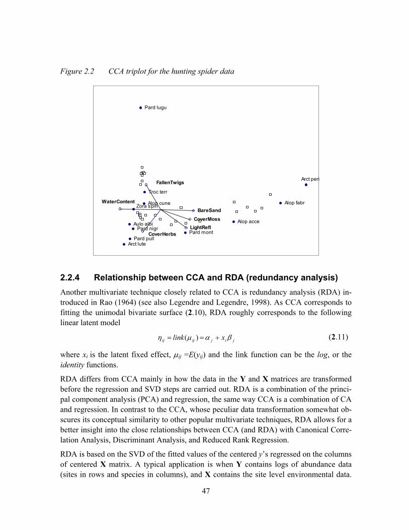
47

Figure 2.2 CCA triplot for the hunting spider data

CoverHerbs

FallenTwigs

LightReflCoverMoss

BareSand

WaterContent

Arct peri

Alop fabr

Alop acce

Pard mont

Alop cune

Troc terr

AuIo albi

Pard pull

Pard nigr

Zora spin

Pard lugu

Arct lute

2.2.4 Relationship between CCA and RDA (redundancy analysis) Another multivariate technique closely related to CCA is redundancy analysis (RDA) in-troduced in Rao (1964) (see also Legendre and Legendre, 1998). As CCA corresponds to fitting the unimodal bivariate surface (2.10), RDA roughly corresponds to the following linear latent model

jijijij xlink βαµη +== )( (2.11)

where xi is the latent fixed effect, µij =E(yij) and the link function can be the log, or the identity functions.

RDA differs from CCA mainly in how the data in the Y and X matrices are transformed before the regression and SVD steps are carried out. RDA is a combination of the princi-pal component analysis (PCA) and regression, the same way CCA is a combination of CA and regression. In contrast to the CCA, whose peculiar data transformation somewhat ob-scures its conceptual similarity to other popular multivariate techniques, RDA allows for a better insight into the close relationships between CCA (and RDA) with Canonical Corre-lation Analysis, Discriminant Analysis, and Reduced Rank Regression.

RDA is based on the SVD of the fitted values of the centered y’s regressed on the columns of centered X matrix. A typical application is when Y contains logs of abundance data (sites in rows and species in columns), and X contains the site level environmental data.

48

More specifically, jijij yyy −=* , and jijij xxx −=* . Then, like in CCA, we obtain BXY *=ˆ , where B is the matrix of regression coefficients of Y* on X* obtained by applying the OLS regression. The SVD decomposition is then carried out on the matrix Y to produce

'ˆ =Y PΛQ .

The output of the procedure contains the following components:

• row scores or site coordinates are the rescaled coordinates for rows of Y (sites), The site coordinates (in the space of Y’s) are 1** QΛYP −= . The fitted site coor-dinates (in the space of X’s) are P

• column scores or species coordinates are representing the columns of Y (species). The species coordinates are obtained from the first few columns of the right-hand singular vectors in Q. Either P* or P can be paired with Q to form a biplot. The de-fault is the JK biplot which emphasize row distances by post multiplying P* or P by the diagonal matrix Λ of singular values.

• The coordinates for the environmental variables in X can be added on the same diagram to form a triplot. These coordinates are formed as correlations of the (fit-ted) site coordinates, P and the columns of environmental variables in X.

2.2.5 Relationship between RDA and Reduced Rank Regression

Recall that RDA is equivalent to the SVD of Y obtained by the OLS of centered Y’s on centered X’s. From (2.5) we can see that the species scores can be obtained by solving the characteristic equation:

2ˆ ˆ| |kλ− =YYS I 0

(where S is a matrix formed of sums of squares and cross-products) which is equivalent to

1 ' 2| |kλ− − =YX XX YXS S S I 0 (2.12)

since ' ' ' -1 ' 2 ' ' -1 'ˆ ˆ [ ]= =Y Y Y X(X X) X Y Y X(X X) X Y . Compare (2.12) to the characteristic equation for the canonical correlation scores for the variables in Y,

1 1 ' 2| |kλ− − − =YY YX XX YXS S S S I 0 (2.13)

Now we see that RDA (and CCA) ignores the correlations among Y’s, when modeling its relationship to X’s, in fact the CCA and RDA analysis is equivalent to that of canonical correlation analysis, when the Syy is identity. The fact that we do not have to deal with Syy is convenient especially when number of species (y variables) is larger than the number of sites minus the number of explanatory variables (n-p), or Syy is not invertible for some

49

other reason. However, what is the justification for (2.12), other than saying that we want to consider the variables in Y and X asymmetrically?

The key point is that in RDA we have a combination of regression and factor analysis, where we seek the factors of matrix Y to be constrained as linear combinations of the ex-planatory variables in X. This does not mean that we completely ignore the correlations between the columns of Y, they will be accounted for to the extent that they are picked by the linear combinations of the explanatory variables fitted to each yi independently. On the contrary, in canonical correlation analysis, we seek pairs of variates uk, vk say, whose cor-relations best pick the correlations between the sets Y and X remaining after the first k-1 pairs (ui, vi) were already accounted for. “Accounting for” here means taking residuals with respect to the extracted components (u, v), thus ensuring that the next pairs would be mutually orthogonal to the pairs already extracted. As was explained, the goal in RDA is quite different.

We can get more insight into this procedure by considering RDA as a special case of the so-called reduced rank regression (RRR). This procedure was considered in Anderson (1951). See also Tso (1981), Davies and Tso (1982) and ter Braak (1994).

The model for the RRR is as follows (ter Braak, 1994):

Y=XM+E (2.14)

Where X (n by p) and Y (n by q) matrices contain observations on n units for q responses and p explanatory variables. M is a p by q matrix of coefficients The errors in E are as-sumed to be uncorrelated across rows and normally distributed with zero expectations and Σ variance-covariance matrix. That is Vec(E) ~ N(0, In⊗Σ), where Vec(E) indicates the column vector in which E is stacked row by row. We further impose a constraint that the p by q matrix of coefficients M is of rank r < min(p,q). This also means that M can be rep-resented (by means of SVD) as a product M=CB’, where C and B are both of full rank r. This leads to the representation Y=XCB’+E or Y=FB’+E, where F contains factor load-ings, and which shows RRR as a combination of regression and factor analysis. There are several methods to obtain the estimates M (see Izenman, 1975; Van der Leeden, 1990) and typically it is carried out under various constraints on the covariance matrix Σ. Here we present the weighted least squares approach which was shown to be equivalent to the MLE under appropriate conditions (section 2.3)

It can be shown (Davies and Tso, 1982) that the weighted error sum of squares allows the following orthogonal decomposition:

||ˆˆ(||||ˆ(||||(|| )ΓYY)ΓYYXM)ΓY r−+−=− , (2.15)

where Y is the matrix of fitted values from the OLS regression, rY is the RRR fit, and Γ is a symmetric positive definite matrix.

50

It follows from (2.15) that the weighted least squares solution to the RRR minimizes the second term of its right-hand side. Using the Eckart-Young theorem (Eckart and Young, 1936), the minimum is obtained from the SVD of the matrix of fitted values, Y weighted by Γ, that is 'PΛΓY Q=ˆ and the minimum of (2.15) is attained by retaining the first r col-umns of the orthogonal matrices P and Q with their associated singular values λi, and

'ˆrr QΛPY rr= .

Now it is obvious that when Γ is taken to be the identity matrix, the solution to the RRR is equivalent to the RDA, as explained in the previous section. When Γ is taken as the squared root of the inverse of the error covariance matrix, estimated by the OLS multi-variate regression, i.e. 2/1ˆ −= olsΣΓ , the scores for the response variables are identical to those obtained by canonical correlation analysis (ter Braak, 1994).

Ter Braak (1994) proposed an “intermediate” way of weighting, where )ˆ( 2/1−= olsdiag ΣΓ , which means that the response variables are weighted with the inverses of their error vari-ances, estimated by OLS. The main purpose of this weighting is that it allows for the in-variance to the linear rescaling of the response variables, such as in canonical correlation analysis, while still permitting for n <p+q. An alternative to weighting is of course stan-dardizing the columns in Y before applying the RRR. For the CCA, when the original Y’s are counts, weighting does not seem to be necessary.

Now that we gave the background on CCA and the related multivariate techniques, we move to our main goal, developing the BMA methodology for such models.

2.3 Implementing BMA for RDA and CCA Variable selection is an important task in CCA given that the number of potential candi-date variables can be very large. ter Braak and Verdonschot (1995) describes a forward selection procedure in CCA based on the Monte-Carlo permutation test (which does not require the assumption of normality). They measure the fit by the sum of all eigenvalues of CCA with each variable as the only additional variable.

One of the goals of the present research is to implement the Bayesian Model Averaging for the selection of variables in CCA and RDA models. I use the MC3 approach (see Raftery et al., 1997; Noble, 2000) where the movements in the associated Markov chain occur only in the model space. I also use the BIC approximation to the Bayes Factors, since we need their ratios for the models M1 and M0 to be able to implement the MC3 al-gorithm. Recall that the BIC approximation gives us the expression for the Bayes Factor, B10= pr(D|M1)/ pr(D|M0) as

nppB o log)(log2 12

10 −−≈ χ

51

where

)},ˆ|(log),ˆ|({log2 012 MDprMDprχ 01 θθ −= ,

is the standard likelihood ratio test statistic when M0 is nested within M1, p0 and p1, are the number of parameters in models M0 and M1. Therefore we need to figure out the likeli-hood and hence the LRT for the CCA and RDA. We will do it by employing the fact that both are special cases of the reduced rank regression, as explained in the previous section.

2.3.1 Computing BIC for the Reduced Rank Regression As was is easy to see, the likelihood for the reduced rank regression problem (2.14) and normal errors with unknown Σ is given by

})(){(||loglog2 '11 XMYΣXMYΣ −−−+= −− trnconstL (2.16)

which has to be maximized with respect to M and Σ, subject to the constraint that rank(M)<min(p,q)= r, as was explained earlier.

Several different representations arise from (2.16) depending on our assumptions about the matrix Σ. As can be easily seen (by invoking the well known identity '( ) || ||tr =A A A , where ||.|| denotes the squared Euclidian norm), the second term in the right-hand side of (2.16) can be written as

||||})(){( 1'1 −− −=−− XM)Σ(YXMYΣXMYtr (2.17)

As noted in ter Braak (1994), there is a direct correspondence between the weighted least squares solution obtained by minimizing (2.15) and the solution obtained by minimizing (2.17) depending on a particular choice of the weight matrix Γ in (2.15). He considers three weighting schemes:

i. Γ is identity, which corresponds to Σ =Iσ2

ii. 21ˆ /ols−= ΣΓ , corresponds to Σ unspecified

iii. )ˆ( 2/1−= olsdiag ΣΓ , corresponds to Σ being a diagonal matrix with unknown vari-ances

2.3.1.1 The case of uncorrelated errors with equal variances (CCA and RDA) The case (i) corresponds to the RDA and the likelihood is maximized by maximizing the part given by (2.17). This case can be divided into two sub-cases.

(ia) 20σ=Σ I , where σ0 is a known constant that has been estimated from the available

data

52

(ib) Σ =Iσ2, where σ is an unknown constant and it has to be estimated from the data

First, let us consider the case (i1). Using the decomposition formula (2.15), and the Eckart and Young theorem (Eckart and Young, 1936) the twice difference of the log likelihoods for the two nested models denoted by the subscripts 1 and 0 will be as follows (see details of the derivation in Appendix A):

∑∑==

−=−r

ii

r

ii λλLL

1

20

1

2101 log2log2 (2.18)

where λ’s are the singular values of the matrix of fitted values olsY . Therefore, the ap-proximation to the Bayes Factor reduces to

[ ]{ }

+−−=

=+−−=

∑∑==

npnp

npLnpLBr

ii

r

ii loglog5.0exp

loglog2loglog25.0exp

01

201

1

21

001110

λλ (2.19)

where p0 and p1 are the number of variables in the model 0 and model 1, respectively. When M is of full rank, this criterion reduces to the difference of the traces of the respec-tive matrices YY' ˆˆ (which was used in ter Braak and Verdonschot, 1995). To use (2.18), one needs to fix the number of components to be retained, which can be a separate prob-lem.

Now consider the case (ib). The maximized twice likelihood is given by: 2 2 '

2

ˆ ˆˆ ˆ2 log( ) log (1/ ) {( ) ( )}ˆlog

L n trn const

σ σ

σ

= − − − −

= − +

Y XM Y XM,

where σ and M are estimated under assumption of M being of rank r<min(p,q). Notice that the second term reduces to a constant since the estimate of σ is based on the residual sum of squares from the reduced rank fit, 2 1 'ˆ ˆˆ ( ) {( ) ( )}nq trσ −= − −Y XM Y XM . Now we can write this expression as

2 1 '

1 ' ( ) ' ( )

1 2 2

1 1

1 2

1

ˆ ˆˆ ( ) {( ) ( )}ˆ ˆ ˆ ˆ ˆ ˆ[ {( ) ( )} {( ) ( )}]

ˆ[ ( ) ]

ˆ[ ( ) ]

r rols ols ols ols

q r

ols i ii i

q

ols ii r

nq tr

n tr tr

n tr

n tr

σ

λ λ

λ

−

−

−

= =

−

= +

= − −

= − − + − −

= Σ + −

= Σ +

∑ ∑

∑

Y XM Y XM

Y Y Y Y Y Y Y Y

53

where λ1> λ2> …>λq are ordered singular values of ˆolsY , and ( )ˆ rY is the reduced rank re-

gression fit (see also the Appendix A). Therefore combining the last two expressions we can write the maximized twice likelihood as follows:

1 2

1

ˆ2 log( ) log [ ( ) ]q

ols ii r

L const n n tr λ−

= +

= + Σ +

∑ (2.20)

As a result, the twice difference of the log likelihoods under (i2) is given by

1 2 1 21 0 1 1 0 0

1 1

ˆ ˆ2 log( ) 2 log( ) log [ ( ) ] log [ ( ) ]q q

i ii r i r

L L n n tr n n trλ λ− −

= + = +

− = Σ + − Σ +

∑ ∑ (2.21)

The approximation to the Bayes Factor, as can be seen from (2.21), is as follows:

0

1

21 1

110

20 0

1

ˆ( )

ˆ( )

nqp

ii r

nqp

ii r

tr nB

tr n

λ

λ

= +

= +

Σ +

=

Σ +

∑

∑ (2.22)

2.3.1.2 The case of unspecified covariance matrix In case (ii) when the covariance matrix is unknown, the term in (2.17) is constant and the likelihood reduces to ||log 1−+ Σnconst , which as was shown in Tso (1981) gives rise to the well-known Wilk’s lambda representation of the likelihood ratio statistic. More spe-cifically, plugging the MLE estimate of Σ into (2.16), and using that tr(AB)=tr(BA) we have:

1/})]ˆ()ˆ)[(ˆ()ˆ{(

})ˆ(]/)ˆ()ˆ)[(ˆ{(})ˆ(ˆ)ˆ{(1''

'1''1

=−−−−=

=−−−−=−−−

−−

ntr

ntrtr

MXYMXYMXYMXY

MXYMXYMXYMXYMXYΣMXY

Finally, it turns out (Tso, 1981) that ∑ =−−+=

r

i inconstL1

12 )1log(log δ , where δ’s are the

canonical correlations. Therefore, for comparing two models we can use the log difference in the corresponding “reduced-rank” Wilk’s statistics:

+−+=− ∑∑

=

−

=

−r

ii

r

iinLL

1

11

1

1001 )1log()1log(log2log2 λλ ,

where λ’s now represent the eigenvalues of the matrix,

[ ] YYYYYYHE 1 '1' )ˆ()ˆ(−− −−= olsols ,

54

assuming that Y’s are centered. Note that the ordinary Wilk’s lambda is computed as

const

qi

|Σ||HE|

|E|1i

ˆ)1( 1 =

+=+=Λ −

=∏ λ (2.23)

therefore we can just use the determinant of Σ matrix when comparing models in the set-ting of full-rank multivariate regression.

2.3.1.3 The case of diagonal covariance matrix (weighted RDA) The case (iii) can be worked out similarly to case ii by observing that the solution to (ii) can be also constructed from a SVD performed on 2/1ˆˆ −ΣY . The fitted values from OLS are multiplied by the square root of covariance matrix estimated from the OLS residuals (see ter Braak, 1994). Consider the singular value decomposition, 'ˆ =YΓ PΛQ . As was already mentioned, we can obtain the estimates for RRR by setting r][ˆ PF = , r][ˆ QΛB Γ= and

r]ˆ[ˆ 11 −−Γ= QΛMC , and our two cases (i) and (ii) naturally arise with Γ set to identity in

(i), and estimated from the OLS residuals 2/1ˆ −Σ in case (ii).

Let us first consider 2/1* ˆˆˆ −= ΣYY . As we saw, the BIC for the case (i) is reduced to the sum of first eigenvalues of YYYY ˆˆˆˆ '*'* = . Now let us see if we can use the same heuristic approach in case (ii).

1 1'* * * '* '2 2

1 ' 1 ' 1

( )

1

ˆ ˆ ˆ ˆ ˆ ˆˆ ˆ( ) ( ) ( )ˆ ˆ ˆ ˆˆ ˆ ( ) ( ) ( )

= q

qi

i

tr tr tr

tr tr tr

Uλ

− −

− − −

=

= = Σ Σ =

= Σ = Σ =

=∑

Y Y Y Y Y Y

Y Y Y Y E H

which is well-known in multivariate analysis as the Lawley-Hotelling statistic, i.e., the sum of eigenvalues of 1−E H . This statistic or its reduced-rank form, ( )rU can be used along with the Wilk’s lambda.

Now, we can consider the case iii similarly by constructing the following reduced rank “Wilk’s”, and “Lawley-Hotelling” statistics, based on the eigenvalues, λ, of

)ˆ( 2/1 HΣΓ −= olsdiag .

*( )

1

rr

ii

U λ=

=∑ and ∏=

−+=Λr

ii

r

1

1)( )1( λ

55

2.3.3 Computing the variance components for CCA and RDA

2.3.3.1 Obtaining the sampling variance components via bootstrap For the unconstrained case of the covariance matrix in RRR, the expressions for the large sample asymptotic variance-covariance matrix of the components of matrices B and C are available in Izenman (1975). In the present research, we chose a different approach using the bootstrap because it does not require any distributional assumptions. In general, let us assume that we need to obtain a bootstrap estimate of variance for the elements of some matrix S. In our context S may contain quantities produced by some variate of the reduced rank regression such as RDA (see 2.2.4) whose output includes the site coordinates P, and the species coordinates Q from the SVD 'ˆ =Y PΛQ .

The variance (and covariance) estimates for the elements of S are obtained as

1 'b b

1

ˆ ( 1) ( )( )B

bB −

• •=

= − − −∑bV (S) S S S S (2.24)

where the Sb is the i-th bootstrap replication of S and 1b

1

B

bB−

•=

= ∑S S

Here the bootstrapped quantities are formed as follows. First we generate a bootstrap rep-licate of the data which can be done in at least three different ways. The first method would be sampling with replacement from the set of rows of the original combined matrix [Y|X]. The second choice is resampling the residuals in the full rank model fitted by OLS, that is ˆ

b ols b= +Y Y E , and finally we can resample residuals from the reduced rank regres-sion. Recall that for the RDA the fitted values are formed simply by using the first r singu-lar vectors in the SVD of '

( ) ( ) ( ) ( )ˆ

r r r r=Y P Λ Q . Therefore in this last case, ( )( )

ˆ rb r b= +Y Y E . In

the present study we use the first approach as it does not depend on any particular model which conforms to our general model averaging methodology. Once the replicated data are formed, we can obtain a bootstrap copy of ˆ

bY by fitting an OLS regression to each

column of Yb and form its SVD, 'ˆb b b b=Y P Λ Q . Now we can obtain the variance of Q by

letting S=Q in (2.24). How would we estimate the variance of the left singular vectors (that are used to form site coordinates in the context of RDA)? While it is tempting to set again S=P in (2.24), it would obviously result in nonsensical results since the rows of bY are randomly sampled from rows of Y and therefore cannot be mapped to the rows of the original set in Y in any meaningful way. Same is true for the relationship between ˆ

bY and

Y and hence between Pb and P. Instead we form the “bootstrap replica of P” by applying the eigenvectors Qb to the “original data” in Y , 1ˆ ˆ

b b b−=P YQ Λ . Notice that this representa-

tion preserves the identity:

56

'ˆ ˆb b b=Y P Λ Q (2.25)

Now the bootstrap estimate of variance of the elements in P is obtained by using (2.24) with ˆ

b=S P .

Another complication that arises in direct using of equation (2.24) is that in our case the quantities of interest are formed from the bootstrapped eigenvectors and therefore are not observable. One obvious problem is that the signs of eigenvectors may flip across sam-ples. What is less obvious is that the eigenvectors of the bootstrapped data can also switch their positions especially when two eigenvalues are close and therefore have to be matched before we can apply the formula (2.24) to the sequence of bootstrapped quanti-ties Qb. Furthermore, even after the eigenvectors are matched, as some authors would ar-gue, we may still want to adjust the coordinates with respect to transformations such as rotations. Such nuisance variation in bootstrap samples can be efficiently suppressed by applying the so-called Procrustes analysis (see Cox and Cox, 1994) to a subset of eigen-vectors. Procrustes analysis is a way to bring a multivariate data set in agreement with some other data of similar composition by applying three types of transformations, rota-tion, and multiplication by a scale and shifting by a constant. In our case we do not have to worry about rescaling or shifting the data, as our only concern is rotation. Note that ro-tation would absorb flipping signs and switching places since we can describe permuta-tions and sign change as an orthogonal matrix of “signed permutations” whose entries contain only elements {-1,0,1} with only one non zero element in each row and column. In Chapter 3 we proposed using a special type of transformation which we call coarsened rotation. This transformation is essentially generated from a rotation matrix by shrinking its elements to 0, 1, or -1. Chapter 3 contains a detailed simulation study of various align-ment schemes. Here we just give a brief outline of the procedure. • perform an SVD on the matrix of fitted values 'ˆ

b b b b=Y P Λ Q as explained in the be-ginning of the section and set ( )r

b=S Q , the first r columns of the matrix of eigenvec-tors that have to be aligned with respect to ( )rQ

• apply Procrustes rotation to Sb to approximate S0 as follows. 1) perform the SVD on the 'UDVSS =b

'o , where bS and 0S contain the row (site)

coordinates for the current bootstrap sample and the raw data, U and V are or-thogonal and D is a diagonal matrix with the singular values.

2) estimate the rotation matrix '=R VU 3) obtained a coarsened version of R, PRC by applying our algorithm from Chapter 3 4) obtain the adjusted Sb as *

b b RC=S S P

Comments:

57

(i) Note that if matrix Sb contains the full set of eigenvectors, Qb, there is no need in Procrustes rotation: since matrix Qb is orthogonal we can simply solve 0SRS =b and ob-

tain obSSR '= and form its coarsened representation, PRC

(ii) Note that we apply the same transformation R=PRC both to the row and column coordinates Q and P obtained via the SVD. The rational for that is the following. As was stated in (2.25) we have the “bootstrap decomposition” of the fitted responses,

'ˆ ˆb b b=Y P Λ Q . Now we can see that with our R defined as a “signed permutation matrix”

and applied to both left and right singular vectors, we have

( )( )'' ' 'ˆ ˆ ˆb b b b b b= =Y P RΛ R Q P R R Λ R Q R

Therefore, our relationship in (2.25) is preserved.

2.3.3.1 Obtaining the variance components due to model selection Classical statistical inference is concerned with estimating the variance of a parameter's estimate, ∆ , conditioned on some pre-selected model. In a Bayesian formulation, the pa-rameter ∆ is considered a random variable and we are concerned with estimating its pos-terior mean and variance. BMA allows us to obtain estimates of the unconditional poste-rior variance of ∆ as shown in the expression below. Here the unconditional variance is obtained as the sum of two components: the average posterior variance conditioned on a particular model (within model variation) and the variance component associated with model selection (between model variation).

)()(

)|(])|[ˆ()|(],|[

)|(2

∆+∆=

∆−∆+∆=

=∆

∑∑betweenwithin

kkkk kk

total

VV

DMprDEDMprMDV

DV

(2.26)

where ],|[ˆkk MDE ∆=∆ and ∑ ∆=∆

k kk DMprDE )|(ˆ]|[ .

In the semi-Bayesian interpretation of BMA, the estimate of the “total variance” of a pa-rameter's estimate, ∆ , can be obtained from the following analogue of (2.26):

)|(])|ˆ[ˆ()|(],|ˆ[ˆ )|ˆ(ˆ 2 DMprDEDMprMDVDV kkkk kk ∆−∆+∆=∆ ∑∑ (2.27)

where the model specific estimates ∆ can be obtained via some classical estimation pro-cedure and the model specific variance ],|ˆ[ kMDV ∆ can be estimated via the available classical method or bootstrap, as explained in 2.3.3.1 Notice that we have to average the model-specific component of variance across all models. When the each of them have to be estimated via bootstrap or other resampling technique, this implies that we have to es-timate all K models in each re-sample, which is computationally unfeasible for a large

58

number of models. To alleviate the problem, researchers (Noble, 2000) use only the full model which may result in biased estimates of the sampling variance. This is particularly true when our quantity of interest, ∆, is a coefficient βi associated with a particular vari-able. Imagine that the model with highest posterior probability does not include the coef-ficient βi, then using its variance from the full model would clearly produce an inflated estimate. To alleviate this problem we propose to shrink the sampling variance of a vari-able-specific quantity (such as a regression coefficient, for example), by multiplying its variance estimated from the full model, by the associated activation probability:

( )ˆ ˆˆ ˆ( | ) ( | ) 0 |within full modelV D V D pr Dβ β β= ≠ (2.28)

The unconditional estimate of the effect is obtained as the weighted average of model spe-cific estimates, ∑ ∆=∆

k kk DMprDE )|(ˆ]|ˆ[ˆ . Of course, in actual computations the true

posterior model probabilities are unknown and we use their estimates obtained via MC3.

Notice that as some models with nontrivial posterior probabilities may not contain the ef-fect ∆ , the “model averaged” estimate will effectively shrink the original classical estimate toward zero.

When computing the variance component due to model selection, we encounter the same problem as we had with the bootstrap estimates of the sampling variability. The eigenvec-tors associated with the SVD of the fitted Y have to be adjusted by applying the Pro-crustes transformation, as explained in section 3.7 of Chapter 3.

2.3.5 Technical details on the algorithm The software (a Visual Basic Macro) has been developed that implements a general MC3 algorithm for multivariate linear regression. The macro can also handle the case of re-duced rank regression. The Markov chain was set following general methodology as ex-plained in section 1.4.2 of the dissertation and is explained in more detail in this section. In the case of CCA, the BIC approximation was used as shown in the previous section for the case of likelihood (ia) and the Bayes Factor reduces to

[ ]{ }

+−−=

=+−−=

∑∑==

npnp

npLnpLBr

ii

r

ii loglog5.0exp

loglog2loglog25.0exp

01

201

1

21

001110

λλ

Therefore, all we need in order to compute the BIC for models M1 and Mo is retaining the

quantity ∑=

r

iik

1

2λ for each proposed model Mk.

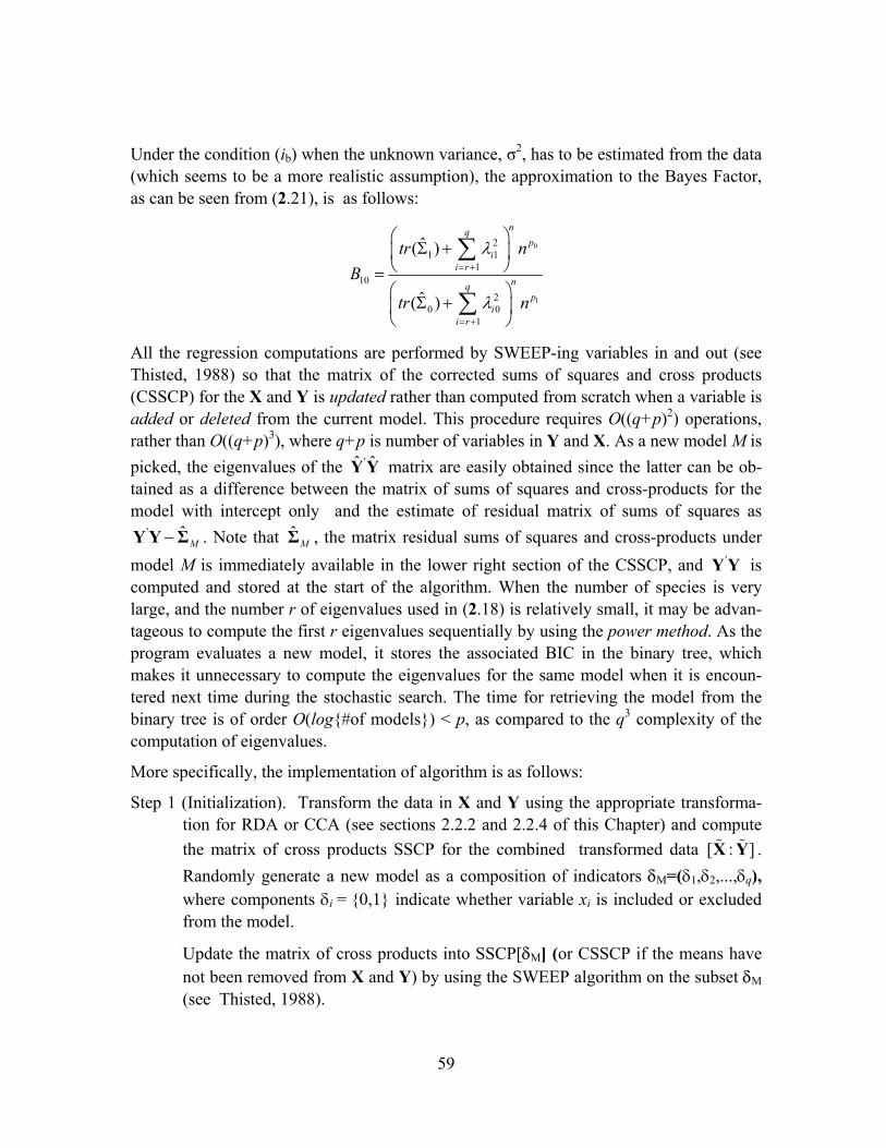
59

Under the condition (ib) when the unknown variance, σ2, has to be estimated from the data (which seems to be a more realistic assumption), the approximation to the Bayes Factor, as can be seen from (2.21), is as follows:

0

1

21 1

110

20 0

1

ˆ( )

ˆ( )

nqp

ii r

nqp

ii r

tr nB

tr n

λ

λ

= +

= +

Σ +

=

Σ +

∑

∑

All the regression computations are performed by SWEEP-ing variables in and out (see Thisted, 1988) so that the matrix of the corrected sums of squares and cross products (CSSCP) for the X and Y is updated rather than computed from scratch when a variable is added or deleted from the current model. This procedure requires O((q+p)2) operations, rather than O((q+p)3), where q+p is number of variables in Y and X. As a new model M is picked, the eigenvalues of the 'ˆ ˆY Y matrix are easily obtained since the latter can be ob-tained as a difference between the matrix of sums of squares and cross-products for the model with intercept only and the estimate of residual matrix of sums of squares as

' ˆM−Y Y Σ . Note that ˆ

MΣ , the matrix residual sums of squares and cross-products under model M is immediately available in the lower right section of the CSSCP, and 'Y Y is computed and stored at the start of the algorithm. When the number of species is very large, and the number r of eigenvalues used in (2.18) is relatively small, it may be advan-tageous to compute the first r eigenvalues sequentially by using the power method. As the program evaluates a new model, it stores the associated BIC in the binary tree, which makes it unnecessary to compute the eigenvalues for the same model when it is encoun-tered next time during the stochastic search. The time for retrieving the model from the binary tree is of order O(log{#of models}) < p, as compared to the q3 complexity of the computation of eigenvalues.

More specifically, the implementation of algorithm is as follows:

Step 1 (Initialization). Transform the data in X and Y using the appropriate transforma-tion for RDA or CCA (see sections 2.2.2 and 2.2.4 of this Chapter) and compute the matrix of cross products SSCP for the combined transformed data [ : ]X Y . Randomly generate a new model as a composition of indicators δM=(δ1,δ2,...,δq), where components δi = {0,1} indicate whether variable xi is included or excluded from the model.

Update the matrix of cross products into SSCP[δM] (or CSSCP if the means have not been removed from X and Y) by using the SWEEP algorithm on the subset δM (see Thisted, 1988).

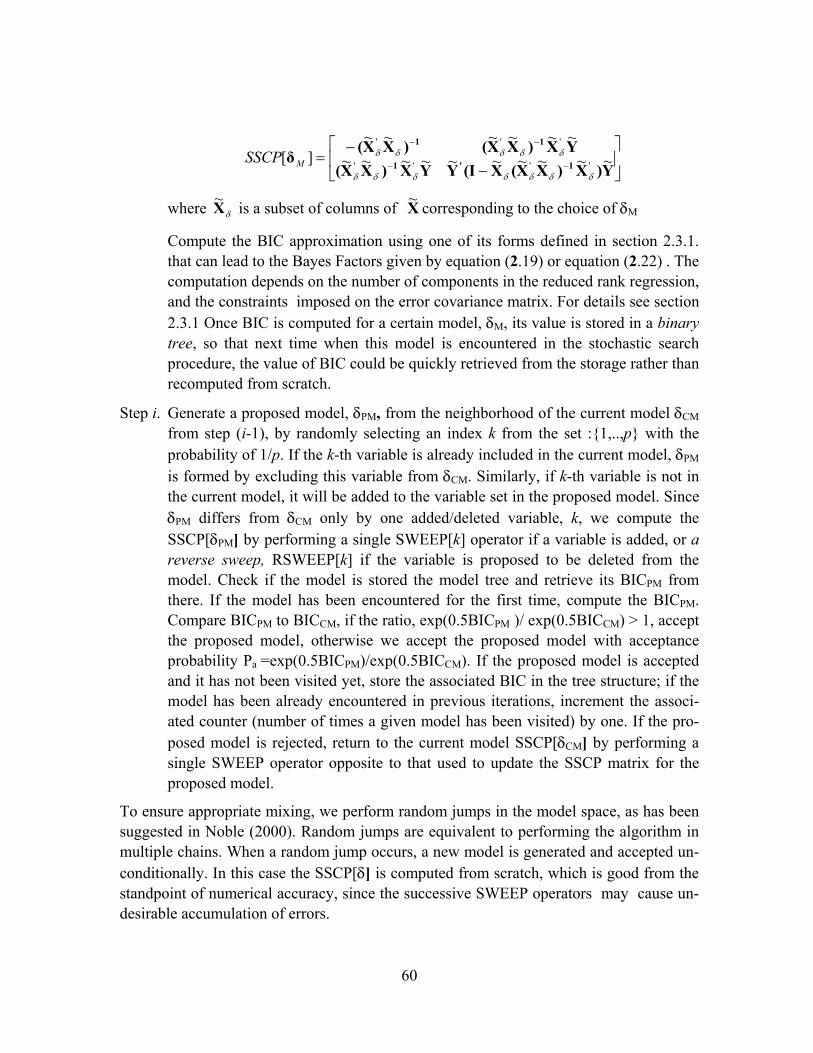
60

−−

=−−

−−

Y)X)XX(X(IYYX)XX(YX)XX()XX(

δ1'1

11

~~~~~~~~~~~~~~~~

][''''

'''

δδδδδδδ

δδδδδMSSCP

where δX~ is a subset of columns of X~ corresponding to the choice of δM

Compute the BIC approximation using one of its forms defined in section 2.3.1. that can lead to the Bayes Factors given by equation (2.19) or equation (2.22) . The computation depends on the number of components in the reduced rank regression, and the constraints imposed on the error covariance matrix. For details see section 2.3.1 Once BIC is computed for a certain model, δM, its value is stored in a binary tree, so that next time when this model is encountered in the stochastic search procedure, the value of BIC could be quickly retrieved from the storage rather than recomputed from scratch.

Step i. Generate a proposed model, δPM, from the neighborhood of the current model δCM from step (i-1), by randomly selecting an index k from the set :{1,..,p} with the probability of 1/p. If the k-th variable is already included in the current model, δPM is formed by excluding this variable from δCM. Similarly, if k-th variable is not in the current model, it will be added to the variable set in the proposed model. Since δPM differs from δCM only by one added/deleted variable, k, we compute the SSCP[δPM] by performing a single SWEEP[k] operator if a variable is added, or a reverse sweep, RSWEEP[k] if the variable is proposed to be deleted from the model. Check if the model is stored the model tree and retrieve its BICPM from there. If the model has been encountered for the first time, compute the BICPM. Compare BICPM to BICCM, if the ratio, exp(0.5BICPM )/ exp(0.5BICCM) > 1, accept the proposed model, otherwise we accept the proposed model with acceptance probability Pa =exp(0.5BICPM)/exp(0.5BICCM). If the proposed model is accepted and it has not been visited yet, store the associated BIC in the tree structure; if the model has been already encountered in previous iterations, increment the associ-ated counter (number of times a given model has been visited) by one. If the pro-posed model is rejected, return to the current model SSCP[δCM] by performing a single SWEEP operator opposite to that used to update the SSCP matrix for the proposed model.

To ensure appropriate mixing, we perform random jumps in the model space, as has been suggested in Noble (2000). Random jumps are equivalent to performing the algorithm in multiple chains. When a random jump occurs, a new model is generated and accepted un-conditionally. In this case the SSCP[δ] is computed from scratch, which is good from the standpoint of numerical accuracy, since the successive SWEEP operators may cause un-desirable accumulation of errors.

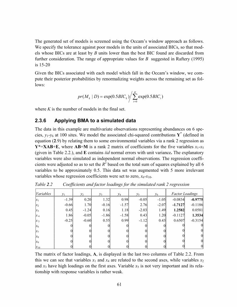
61

The generated set of models is screened using the Occam’s window approach as follows. We specify the tolerance against poor models in the units of associated BICs, so that mod-els whose BICs are at least by B units lower than the best BIC found are discarded from further consideration. The range of appropriate values for B suggested in Raftery (1995) is 15-20

Given the BICs associated with each model which fall in the Occam’s window, we com-pute their posterior probabilities by renormalizing weights across the remaining set as fol-lows:

∑=

=K

iikk BICBICDMpr

0)5.0exp()5.0exp()|(

where K is the number of models in the final set.

2.3.6 Applying BMA to a simulated data The data in this example are multivariate observations representing abundances on 6 spe-cies, y1-y6 at 100 sites. We model the associated chi-squared contributions Y* (defined in equation (2.9) by relating them to some environmental variables via a rank 2 regression as Y*=XAB+E, where AB=M is a rank 2 matrix of coefficients for the five variables x1-x5 (given in Table 2.2.), and E contains iid normal errors with unit variance. The explanatory variables were also simulated as independent normal observations. The regression coeffi-cients were adjusted so as to set the R2 based on the total sum of squares explained by all 6 variables to be approximately 0.5. This data set was augmented with 5 more irrelevant variables whose regression coefficients were set to zero, x6-x10.

Table 2.2 Coefficients and factor loadings for the simulated rank 2 regression

Variables y1 y2 y3 y4 y5 y6 Factor Loadings x1 -1.39 0.20 1.32 0.98 -0.05 -1.05 -0.0834 -0.9775x2 -0.66 1.70 -0.16 -1.57 2.76 -2.07 -1.7127 -0.1186x3 0.45 -1.24 0.16 1.18 -2.03 1.49 1.2582 0.0581x 4 1.86 -0.05 -1.86 -1.58 0.43 1.20 -0.1127 1.3534x 5 -0.25 -0.60 0.55 0.99 -1.12 0.43 0.6507 -0.3154x6 0 0 0 0 0 0 0 0x7 0 0 0 0 0 0 0 0x8 0 0 0 0 0 0 0 0x9 0 0 0 0 0 0 0 0x10 0 0 0 0 0 0 0 0

The matrix of factor loadings, A, is displayed in the last two columns of Table 2.2. From this we can see that variables x1 and x4 are related to the second axes, while variables x2

and x3 have high loadings on the first axes. Variable x5 is not very important and its rela-tionship with response variables is rather weak.

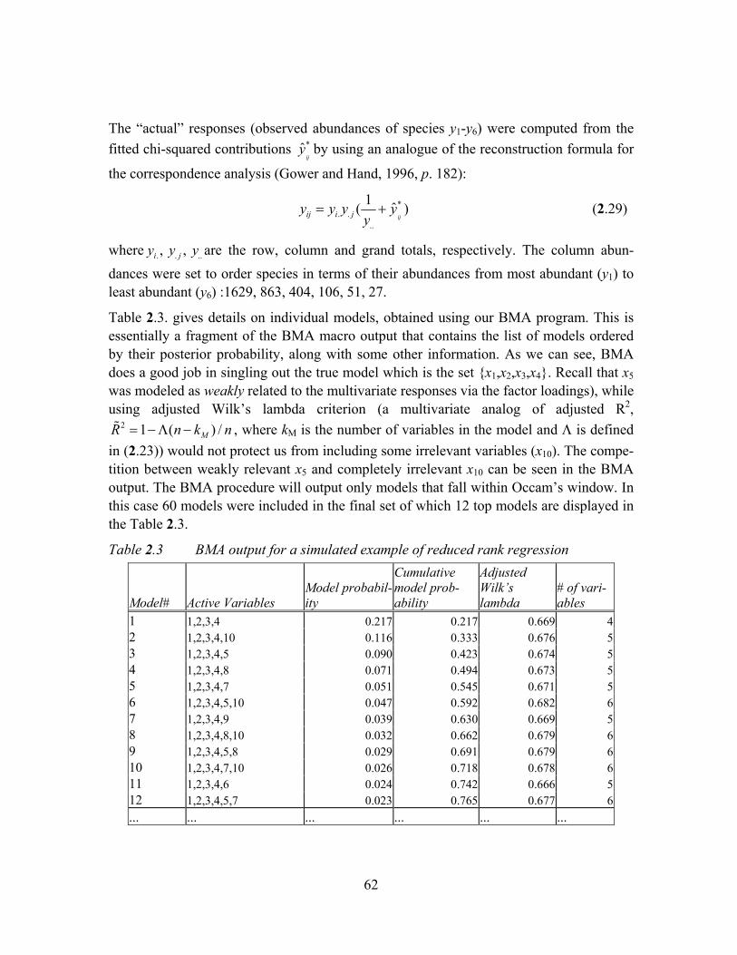
62

The “actual” responses (observed abundances of species y1-y6) were computed from the fitted chi-squared contributions *ˆ

ijy by using an analogue of the reconstruction formula for

the correspondence analysis (Gower and Hand, 1996, p. 182):

*. .

..

1 ˆ( )ijij i jy y y y

y= + (2.29)

where . . .., , i jy y y are the row, column and grand totals, respectively. The column abun-dances were set to order species in terms of their abundances from most abundant (y1) to least abundant (y6) :1629, 863, 404, 106, 51, 27.

Table 2.3. gives details on individual models, obtained using our BMA program. This is essentially a fragment of the BMA macro output that contains the list of models ordered by their posterior probability, along with some other information. As we can see, BMA does a good job in singling out the true model which is the set {x1,x2,x3,x4}. Recall that x5 was modeled as weakly related to the multivariate responses via the factor loadings), while using adjusted Wilk’s lambda criterion (a multivariate analog of adjusted R2,

2 1 ( ) /MR n k n= −Λ −% , where kM is the number of variables in the model and Λ is defined in (2.23)) would not protect us from including some irrelevant variables (x10). The compe-tition between weakly relevant x5 and completely irrelevant x10 can be seen in the BMA output. The BMA procedure will output only models that fall within Occam’s window. In this case 60 models were included in the final set of which 12 top models are displayed in the Table 2.3.

Table 2.3 BMA output for a simulated example of reduced rank regression

Model# Active Variables Model probabil-ity

Cumulative model prob-ability

Adjusted Wilk’s lambda

# of vari-ables

1 1,2,3,4 0.217 0.217 0.669 42 1,2,3,4,10 0.116 0.333 0.676 53 1,2,3,4,5 0.090 0.423 0.674 54 1,2,3,4,8 0.071 0.494 0.673 55 1,2,3,4,7 0.051 0.545 0.671 56 1,2,3,4,5,10 0.047 0.592 0.682 67 1,2,3,4,9 0.039 0.630 0.669 58 1,2,3,4,8,10 0.032 0.662 0.679 69 1,2,3,4,5,8 0.029 0.691 0.679 610 1,2,3,4,7,10 0.026 0.718 0.678 611 1,2,3,4,6 0.024 0.742 0.666 512 1,2,3,4,5,7 0.023 0.765 0.677 6... ... ... ... ... ...

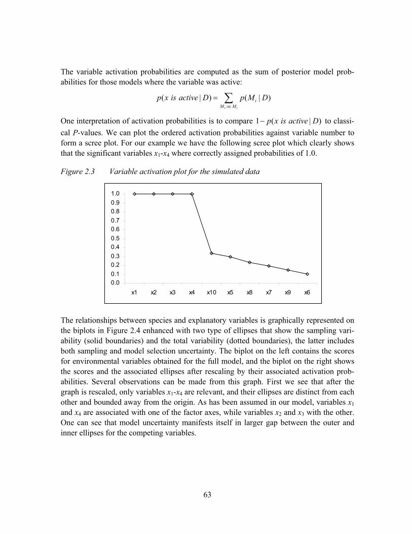
63

The variable activation probabilities are computed as the sum of posterior model prob-abilities for those models where the variable was active:

:( | ) ( | )

i i

iM x M

p x is active D p M D∈

= ∑

One interpretation of activation probabilities is to compare 1 ( | )p x is active D− to classi-cal P-values. We can plot the ordered activation probabilities against variable number to form a scree plot. For our example we have the following scree plot which clearly shows that the significant variables x1-x4 where correctly assigned probabilities of 1.0.

Figure 2.3 Variable activation plot for the simulated data

0.00.10.20.30.40.50.60.70.80.91.0

x1 x2 x3 x4 x10 x5 x8 x7 x9 x6

The relationships between species and explanatory variables is graphically represented on the biplots in Figure 2.4 enhanced with two type of ellipses that show the sampling vari-ability (solid boundaries) and the total variability (dotted boundaries), the latter includes both sampling and model selection uncertainty. The biplot on the left contains the scores for environmental variables obtained for the full model, and the biplot on the right shows the scores and the associated ellipses after rescaling by their associated activation prob-abilities. Several observations can be made from this graph. First we see that after the graph is rescaled, only variables x1-x4 are relevant, and their ellipses are distinct from each other and bounded away from the origin. As has been assumed in our model, variables x1 and x4 are associated with one of the factor axes, while variables x2 and x3 with the other. One can see that model uncertainty manifests itself in larger gap between the outer and inner ellipses for the competing variables.

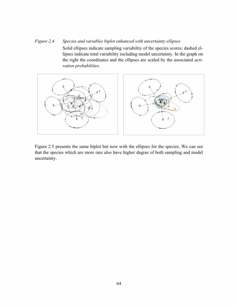
64

Figure 2.4 Species and variables biplot enhanced with uncertainty ellipses Solid ellipses indicate sampling variability of the species scores; dashed el-lipses indicate total variability including model uncertainty. In the graph on the right the coordinates and the ellipses are scaled by the associated acti-vation probabilities.

y1

y2

y3

y4

y5

y6x1

x2

x3

x4

x5x6x7 x8x9

x10x5x8

x10y1

y2

y3

y4

y5

y6x1

x2

x3

x4

x5

x6

x7x8

x9

x10

Figure 2.5 presents the same biplot but now with the ellipses for the species. We can see that the species which are more rare also have higher degree of both sampling and model uncertainty.

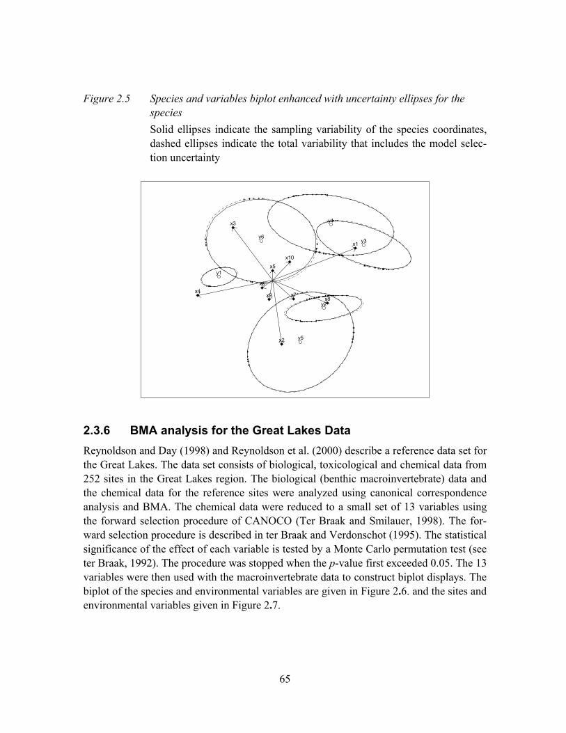
65

Figure 2.5 Species and variables biplot enhanced with uncertainty ellipses for the species Solid ellipses indicate the sampling variability of the species coordinates, dashed ellipses indicate the total variability that includes the model selec-tion uncertainty

y1

y2

y3

y4

y5

y6x1

x2

x3

x4

x5

x6

x7x8

x9

x10

2.3.6 BMA analysis for the Great Lakes Data Reynoldson and Day (1998) and Reynoldson et al. (2000) describe a reference data set for the Great Lakes. The data set consists of biological, toxicological and chemical data from 252 sites in the Great Lakes region. The biological (benthic macroinvertebrate) data and the chemical data for the reference sites were analyzed using canonical correspondence analysis and BMA. The chemical data were reduced to a small set of 13 variables using the forward selection procedure of CANOCO (Ter Braak and Smilauer, 1998). The for-ward selection procedure is described in ter Braak and Verdonschot (1995). The statistical significance of the effect of each variable is tested by a Monte Carlo permutation test (see ter Braak, 1992). The procedure was stopped when the p-value first exceeded 0.05. The 13 variables were then used with the macroinvertebrate data to construct biplot displays. The biplot of the species and environmental variables are given in Figure 2.6. and the sites and environmental variables given in Figure 2.7.

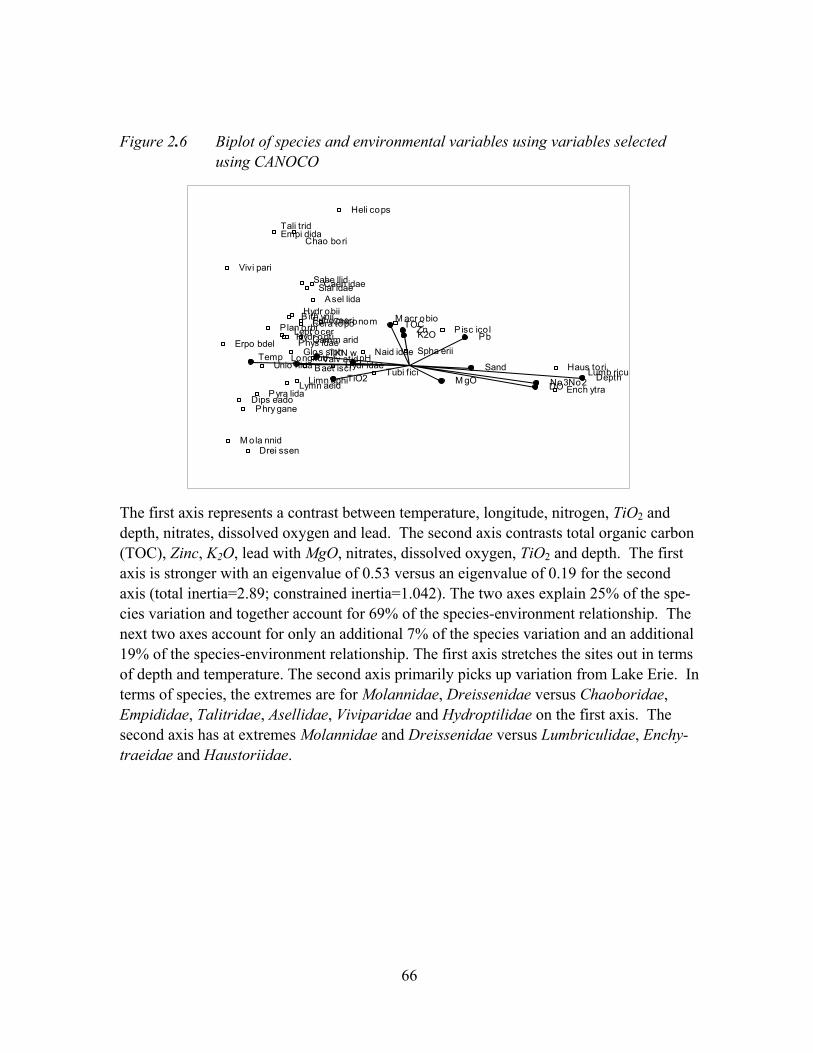
66

Figure 2.6 Biplot of species and environmental variables using variables selected using CANOCO

Longitud

Depth

Temp Sand

K2O

M gO

Pb

TiO2

TOC Zn

DO No3No2

pH TKN w

Tubi fici Haus tori

Drei ssen

Chir onom

Spha erii

Lumb ricu

Naid idae

Ench ytra

Asel lida

Gamm arid

Valv atid

Sabe llid

Plan orbi

Hydr idae

Ephe meri Hydr obii

Lept ocer Phys idae

Cera topo

Chao bori

Glos siph Unio nida

Erpo bdel

B ith ynii

Lymn aeid

Hydr opti

Tali trid

Caen idae Sial idae

Limn ephi

P isc ico l

Phry gane

M acr obio

Empi dida

Heli cops

Baet isci

Dips eado

M ola nnid

Pyra lida

Vivi pari

The first axis represents a contrast between temperature, longitude, nitrogen, TiO2 and depth, nitrates, dissolved oxygen and lead. The second axis contrasts total organic carbon (TOC), Zinc, K2O, lead with MgO, nitrates, dissolved oxygen, TiO2 and depth. The first axis is stronger with an eigenvalue of 0.53 versus an eigenvalue of 0.19 for the second axis (total inertia=2.89; constrained inertia=1.042). The two axes explain 25% of the spe-cies variation and together account for 69% of the species-environment relationship. The next two axes account for only an additional 7% of the species variation and an additional 19% of the species-environment relationship. The first axis stretches the sites out in terms of depth and temperature. The second axis primarily picks up variation from Lake Erie. In terms of species, the extremes are for Molannidae, Dreissenidae versus Chaoboridae, Empididae, Talitridae, Asellidae, Viviparidae and Hydroptilidae on the first axis. The second axis has at extremes Molannidae and Dreissenidae versus Lumbriculidae, Enchy-traeidae and Haustoriidae.

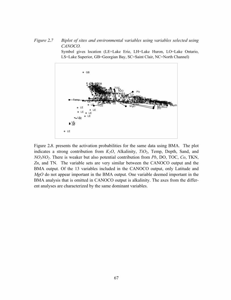
67

Figure 2.7 Biplot of sites and environmental variables using variables selected using CANOCO. Symbol gives location (LE=Lake Erie, LH=Lake Huron, LO=Lake Ontario, LS=Lake Superior, GB=Georgian Bay, SC=Saint Clair, NC=North Channel)

Longitud

Depth

Temp Sand

K2O

M gO

Pb

TiO2

TOC Zn

DO No3No2

pH TKN w LH

LE

LE

SC

LELE LE

LE

LELELELELE

LELELE

LE

LELE

LELELE

LELE

LE

LE

LE LE

LE

LE

LE

LELE

LE

LE

LE

LE

LE

LE

LE

LE

LE

LE

LOLOLO

LOLOLO LO

LO

LOLO

LOLHLH

LHLH

LHLH

LHLHLH

LHLH

LHLHLH

LH LHGB

GBGB

GBGBGB

GBGB

GB

GB

GBGBGB GB

GBGB

GB

GB

GBGBGB

GB

GB

GBGB

GB GBGBGB

GB

GB

GB

GB

GB

GBGB GBGB

GBLOLO

LOLO

LOLO LO

LOLO

LOLO

LOLO

LO

LO

LOLONC

NCNC

NCNC

NC

NC

NCNC

NCNC

NC

NC

NC

NC

NCNCNC NC

NC

NC

NC

NCNCNC

NCNC

NC

GB

GBGBGB

GB

GB

GBGB

GBGBGB

GB

GBGB

GB

GB

GB

GBGB

GB

GBGB

NCNCNC

NC

NC

NC

NCNCLS

LSLS

LSLS

LS

LS

LS

LSLSLS

LS

LSLS

LSLSLSLS

LSLS

LS LSLS LSLSLSLS

LSLSLSLSLM LM LMLM LMLMLMLMLM LMLM LMLM LMLMLMLMLMLM LM

LM

LM

LM

LMLM LMLMLMLMLM

LMLM

LMLMLM LMLM

Figure 2.8. presents the activation probabilities for the same data using BMA. The plot indicates a strong contribution from K2O, Alkalinity, TiO2, Temp, Depth, Sand, and NO3NO2. There is weaker but also potential contribution from Pb, DO, TOC, Co, TKN, Zn, and TN. The variable sets are very similar between the CANOCO output and the BMA output. Of the 13 variables included in the CANOCO output, only Latitude and MgO do not appear important in the BMA output. One variable deemed important in the BMA analysis that is omitted in CANOCO output is alkalinity. The axes from the differ-ent analyses are characterized by the same dominant variables.

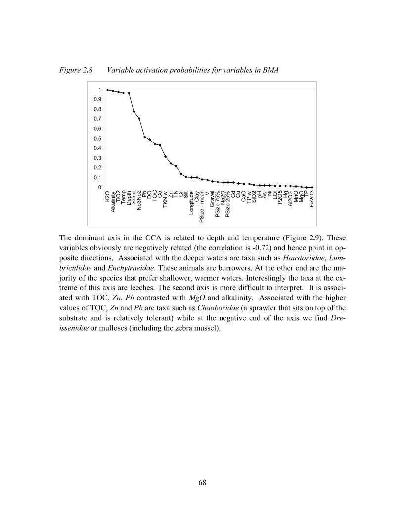
68

Figure 2.8 Variable activation probabilities for variables in BMA

0

0.1

0.2

0.3

0.4

0.5

0.6

0.7

0.8

0.9

1

K2O

Alka

linity

TiO

2Te

mp

Dep

thSa

ndN

o3N

o2 Pb DO

TOC

Co

TKN

w Zn TN Cr

Silt

Long

itude

Cla

yPS

ize

- mea

n VG

rave

lPS

ize

75%

Na2

OPS

ize

25% Cd

Cu

CaO

TP w

SiO

2pH As N

iLO

IP2

O5

Hg

Al2O

3M

nOM

gO TPFe

2O3

The dominant axis in the CCA is related to depth and temperature (Figure 2.9). These variables obviously are negatively related (the correlation is -0.72) and hence point in op-posite directions. Associated with the deeper waters are taxa such as Haustoriidae, Lum-briculidae and Enchytraeidae. These animals are burrowers. At the other end are the ma-jority of the species that prefer shallower, warmer waters. Interestingly the taxa at the ex-treme of this axis are leeches. The second axis is more difficult to interpret. It is associ-ated with TOC, Zn, Pb contrasted with MgO and alkalinity. Associated with the higher values of TOC, Zn and Pb are taxa such as Chaoboridae (a sprawler that sits on top of the substrate and is relatively tolerant) while at the negative end of the axis we find Dre-issenidae or mulloscs (including the zebra mussel).

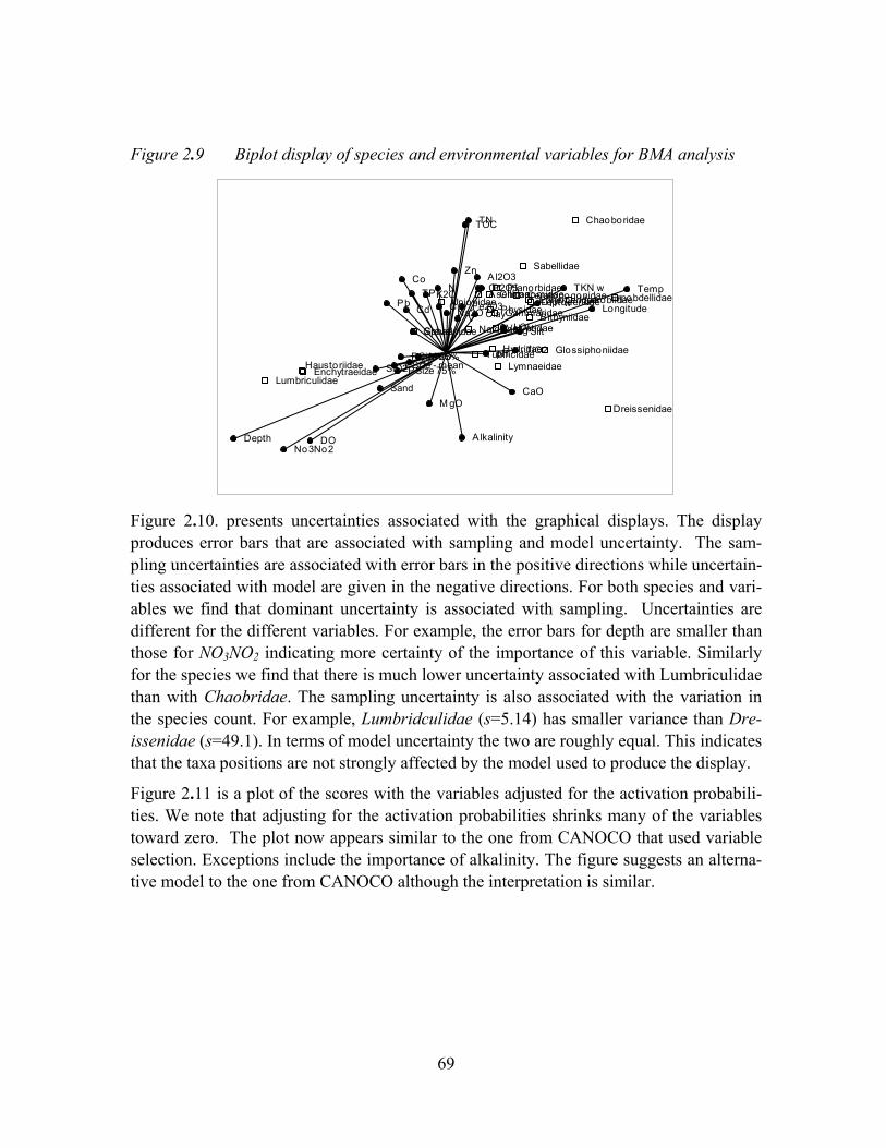
69

Figure 2.9 Biplot display of species and environmental variables for BMA analysis

TP wTKN w

pH

No3No2DO Alkalinity

Zn

V

TP

TOC

TiO2

TN

SiO2

P2O5Pb

Ni

Na2O

M nO

M gO

LOI

K2O

Hg

Fe2O3Cu

CrCo

Cd

CaO

As

Al2O3

PSize 75%PSize 25%

PSize - mean

Clay

Silt

Sand

Gravel

Temp

Depth

Longitude

Lymnaeidae

Bithyniidae

ErpobdellidaeUnionidae

Glossiphoniidae

Chaoboridae

CeratopogonidaePhysidae

LeptoceridaeHydrobiidaeEphemeridae

Hydridae

Planorbidae

Sabellidae

ValvatidaeGammaridae

Asellidae

Enchytraeidae

Naididae

Lumbriculidae

Sphaeriidae

Chironomidae

Dreissenidae

HaustoriidaeTubificidae

Figure 2.10. presents uncertainties associated with the graphical displays. The display produces error bars that are associated with sampling and model uncertainty. The sam-pling uncertainties are associated with error bars in the positive directions while uncertain-ties associated with model are given in the negative directions. For both species and vari-ables we find that dominant uncertainty is associated with sampling. Uncertainties are different for the different variables. For example, the error bars for depth are smaller than those for NO3NO2 indicating more certainty of the importance of this variable. Similarly for the species we find that there is much lower uncertainty associated with Lumbriculidae than with Chaobridae. The sampling uncertainty is also associated with the variation in the species count. For example, Lumbridculidae (s=5.14) has smaller variance than Dre-issenidae (s=49.1). In terms of model uncertainty the two are roughly equal. This indicates that the taxa positions are not strongly affected by the model used to produce the display.

Figure 2.11 is a plot of the scores with the variables adjusted for the activation probabili-ties. We note that adjusting for the activation probabilities shrinks many of the variables toward zero. The plot now appears similar to the one from CANOCO that used variable selection. Exceptions include the importance of alkalinity. The figure suggests an alterna-tive model to the one from CANOCO although the interpretation is similar.

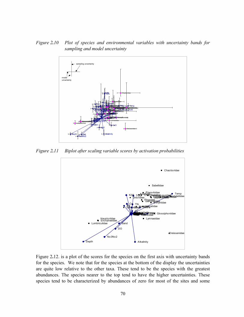
70

Figure 2.10 Plot of species and environmental variables with uncertainty bands for sampling and model uncertainty

TP wTKN w

pH

No3No2DO Alkalinity

Zn

V

TP

TOC

TiO2

TN

SiO2

P2O5Pb

Ni

Na2O

MnO

MgO

LOI

K2O

Hg

Fe2O3Cu

CrCo

Cd

CaO

As

Al2O3

PSize 75%PSize 25%

PSize - mean

ClaySilt

Sand

Gravel

Temp

Depth

Longitude

Lymnaeidae

Bithyniidae

ErpobdellidaeUnionidae

Glossiphoniidae

Chaoboridae

CeratopogonidaePhysidae

LeptoceridaeHydrobiidaeEphemeridae

Hydridae

Planorbidae

Sabellidae

Valvatidae

Gammaridae

Asellidae

Enchytraeidae

Naididae

Lumbriculidae

Sphaeriidae

Chironomidae

Dreissenidae

Haustoriidae

Tubificidae

sampling uncertainty

modeluncertainty

Figure 2.11 Biplot after scaling variable scores by activation probabilities

Longitude

Depth

Temp

Gravel

Sand

SiltClayPSize - meanPSize 25%PSize 75%Al2O3AsCaOCd

Co

CrCuFe2O3Hg

K2O

LOIM gOM nONa2ONi

Pb

P2O5SiO2

TN

TiO2

TOC

TPV

Zn

Alkalinity

DO

No3No2

pH

TKN w

TP wTubificidaeHaustoriidae

Dreissenidae

Chironomidae

Sphaeriidae

Lumbriculidae

Naididae

Enchytraeidae

Asellidae

Gammaridae

Valvatidae

Sabellidae

Planorbidae

Hydridae

EphemeridaeHydrobiidaeLeptoceridaePhysidae

Ceratopogonidae

Chaoboridae

Glossiphoniidae

Unionidae Erpobdellidae

Bithyniidae

Lymnaeidae

Figure 2.12. is a plot of the scores for the species on the first axis with uncertainty bands for the species. We note that for the species at the bottom of the display the uncertainties are quite low relative to the other taxa. These tend to be the species with the greatest abundances. The species nearer to the top tend to have the higher uncertainties. These species tend to be characterized by abundances of zero for most of the sites and some

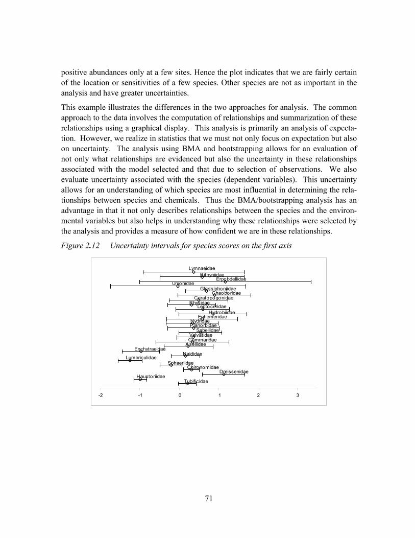
71

positive abundances only at a few sites. Hence the plot indicates that we are fairly certain of the location or sensitivities of a few species. Other species are not as important in the analysis and have greater uncertainties.

This example illustrates the differences in the two approaches for analysis. The common approach to the data involves the computation of relationships and summarization of these relationships using a graphical display. This analysis is primarily an analysis of expecta-tion. However, we realize in statistics that we must not only focus on expectation but also on uncertainty. The analysis using BMA and bootstrapping allows for an evaluation of not only what relationships are evidenced but also the uncertainty in these relationships associated with the model selected and that due to selection of observations. We also evaluate uncertainty associated with the species (dependent variables). This uncertainty allows for an understanding of which species are most influential in determining the rela-tionships between species and chemicals. Thus the BMA/bootstrapping analysis has an advantage in that it not only describes relationships between the species and the environ-mental variables but also helps in understanding why these relationships were selected by the analysis and provides a measure of how confident we are in these relationships.

Figure 2.12 Uncertainty intervals for species scores on the first axis

TubificidaeHaustoriidae

DreissenidaeChironomidae

SphaeriidaeLumbriculidae

NaididaeEnchytraeidae

AsellidaeGammaridaeValvatidae

SabellidaePlanorbidaeHydridae

EphemeridaeHydrobiidae

LeptoceridaePhysidae

CeratopogonidaeChaoboridae

GlossiphoniidaeUnionidae

ErpobdellidaeBithyniidae

Lymnaeidae

-2 -1 0 1 2 3

72

Chapter 3 Alignment of Eigenvectors when Estimating Variance Components

3.1. Background and motivation Analysis of multivariate data inherently involves computing eigenvectors of some matrix derived from the data. For example, in principal components analysis (PCA) we analyze the eigenvectors of a p by p covariance matrix ˆ /( 1)n −'Σ = (X - X) (X - X) , in canonical discriminant analysis (CDA) we are concerned with the eigenvectors of 1−W B where W and B are the within and between group covariance matrices, respectively. The asymp-totic formulas for the standard errors of the elements of these eigenvectors are available for the case of normally distributed data: for PCA see Jackson (1991) and the references therein. Formulas for the standard errors of canonical discriminant functions are given in Krzanowski (1989). Izenman (1975) derived formulas for the standard errors of reduced rank regression estimates, which are essentially functions of the first k eigenvectors asso-ciated with canonical correlation analysis. However, computing the variances of the ei-genvectors of such matrices under no distributional assumptions is difficult and requires using resampling methods such as the bootstrap and jackknife (see for example, Weinberg & Carroll, 1984; Krzanowski & Radley, 1989).

It should be noted that the need to estimate variances of eigenvectors arises not only in formal hypothesis testing but also in presenting exploratory graphs that accompany many multivariate methods. These plots reflect the configurations of data in a low dimensional space, such as the scatter plot of the data in the space spanned by the first few principal components (or main factors in factor analysis models), a plot of canonical means or scores in CDA, or a configuration of objects produced by multidimensional scaling (MDS). Naturally, these coordinates are functions of eigenvectors associated with certain matrices derived from the data, and therefore estimated covariance matrices associated with these eigenvectors would be used in constructing confidence or probability ellipses for the coordinates, which are an important aid in the visual assessment of the stability of the estimated configuration. In the case of multivariate normal data, ellipses are con-structed for axes x and y, say, based on the estimated covariance matrices and assuming an F distribution for the distribution of the associated quadratic forms. More technically, given the unbiased estimate of the population covariance matrix, Sθ for a pair of coordi-nates x, and y of a single row in the “configuration matrix”, θ,

2

2x xy x y

xy x y y

s r s sS

r s s sθ

=

73

and the sample centroid ( , )x y=θ θ θ , the boundaries of the (1-α)% confidence region for in the (x,y) plane may be expressed by the equation (n is the sample size):

' 1(2, 2)

2( 1)( ) ( )( 2) nn F

n nθ−

−−

− − =−

θ θ S θ θ (3.1)

The (1-α)% probability (or tolerance) region is obtained by simply removing n from the denominator in the right hand part of (3.1) (an example of such graph is in Figure 2.4). These regions are readily obtained in statistical packages such as SYSTAT and SAS In-sight, sometimes using a chi-square distribution instead of the F distribution. In cases where the coordinates are associated with observed quantities, the intervals are accurate. However, in cases where the coordinates are latent variables (components, factors, dis-criminant axes) the accuracy has been questioned. For example, Krzanowski (1989) ar-gued that the confidence ellipses for the canonical coordinates of the group means are rou-tinely computed using incorrect variances that do not take into account the sampling vari-ability in the elements of discriminant functions (computed from the eigenvectors of

1−W B ). An alternative to the use of the F distribution is to use a nonparametric approach based on the bootstrap or jackknife. For example, the bootstrap estimate of the covariance matrix associated with eigenvector θ is computed as follows:

( )( )'

1 1

1 1ˆ ˆ ˆ ˆ ˆ ˆ, ,1

B B

b bb bB B= =

= =− ∑ ∑* * * * * * *

θ . . . bS θ -θ θ -θ θ θ (3.2)

where ˆb*θ is the estimate of the eigenvector obtained in the bth bootstrap sample.

When variances of eigenvectors are estimated based on data resampling algorithms, an additional problem arises in that the natural sampling variability may cause eigenvectors to flip signs and even swap their positions, especially if some population eigenvalues hap-pen to be close enough. Several methods of aligning eigenvectors have been proposed in the literature as a way of adjusting for the sign and swapping problems. One approach to variance estimation (Clarkson, 1979; Ichikawa & Konishi, 1995, further referred to as CL) was developed in the context of factor analysis model and was motivated by the in-determinacy inherent in such models. In factor analysis, a p by k matrix of factor loadings U is estimated from the model for the covariance matrix '= +Σ UΦU Ψ , where Φ is a positive definite correlation matrix, and Ψ is a diagonal matrix containing the variances associated with the unique components of the variables. In Clarkson’s method the initial or reference loadings matrix computed using the full data is denoted UR. For the i-th re-sample, columns of U (the subscript i is suppressed for convenience) generated by an ap-propriate resampling method may be permuted and the signs of the columns in U may be switched so as to make U as close as possible to the reference matrix, UR. While this method was shown to produce reliable results in many simulation experiments, it is com-

74

putationally very intensive for solutions involving more than 10 factors, since it requires evaluation of some functional for each of the k! possible permutations.

Another approach applies the Procrustes transformation to the p by k matrix U so as to minimize the associated sum of squares of deviations between U and UR. The Procrustes transformation (PT) is a combination of translation, scaling and rotation (see Cox & Cox, 1994) applied to a multivariate data Y so as to make their multivariate configuration as close as possible to that of some reference data set (of same dimensionality) Z, the cri-terion of proximity being tr '(Y - Z) (Y - Z) (a more detailed description is in section 3.3.) Some authors suggest using Procrustes transformation to adjust the raw configurations estimated from the bootstrap or jackknife samples so as to remove the part of the variabil-ity in the re-sampled data that does not reflect the actual sampling variability. For example in Krzanowski & Radley (1989) jackknife and bootstrap methods are used with the Pro-crustes rotation applied to the resultant configurations obtained with the canonical variates analysis to produce the best fit with the original configuration. They had found that when the Procrustes rotation is applied to jackknife and bootstrap replicates, the effects of vary-ing frames of reference are removed, and the results accentuate the elongation of confi-dence regions.

In the present research we are concerned with estimation of standard errors of singular vectors associated with a SVD of some n by p data matrix Y, when they are estimated by bootstrap. Consider a p by p matrix U and an n by p matrix V of singular vectors associ-ated with a singular value decomposition

1/ 1 'n= −X (X - X) = VΛU% (3.3)

where 2Λ is the matrix of eigenvalues associated with Σ (our notation here differs from the conventional use of U as left singular vectors and V as right singular vectors). This leads to the standard PCA based on the covariance matrix, Σ . A natural graphical repre-sentation associated with this SVD is the PCA biplot. In a biplot, cases are represented by the first two columns of VΛ and variables are represented by the first two columns of U . Our goal is to evaluate the accuracy of different alignment schemes used when obtaining variance estimates via bootstrap. Once we develop some understanding of alignment in a relatively simple case of PCA, we can apply this to a more complicated, however concep-tually similar cases of RDA and CCA. The only difference between PCA and these meth-ods is that in the latter case the SVD is applied to the matrix of fits 'ˆ =Y VΛU . Recall from section 2.2.4 that the biplot coordinates for the sites can be formed as the first two columns [2]( )VΛ and the coordinates for the species are U[2] (for a JK biplot). Below we list some issues that will be addressed in the present study:

(i) Notice that the relationship between the left and right singular vectors, V and U which together form the observed (or fitted) data in the decomposition 'ˆ =Y VΛU , has to

75

be preserved when aligning either of them. For example, if the aligned species coordinates for a bootstrap sample Xb are *

bU , then we can derive the aligned singular vectors *bV co-

ordinates by inverting the “bootstrap identity” (2.25) (assuming the aligned vectors in U* are still orthogonal) as * 1ˆ

b b−YU Λ . Alternatively, if we form the aligned sites’ coordinates

first, this would predetermine the aligned species coordinates. Which of them should be aligned first? The existing literature does not provide an answer, probably because in many applications there is only one set of vectors to be aligned and the duality between the left and right vectors is not well understood. One may even surmise that aligning the row scores (left singular vectors) would be a more reliable procedure because it is based on matching n cases, while the column scores are matched only by p elements, and typi-cally p < n.

(ii) Another question is how many axes should be used for obtaining the alignment? In the factor analysis literature, this is not an issue, because the number of factors is pre-specified, however when aligning coordinates in PCA and related methods, we can choose as many axes as the number of singular vectors. The fact that we may be interested in only two axes when plotting the site and species coordinates does not mean that only two axes should be used for alignment. In a situation when the third eigenvalue is close to the sec-ond eigenvalue, it may happen that the second axes will swap places with the third and we should be able to detect that.

(iii) It would be desirable if the actual values of the singular vectors (and singular val-ues in Λ) were preserved after alignment. This corresponds to our intuitive understanding of the behavior of singular vectors in the data resampling process. Using a “strong” method of alignment such as Procrustes transformation could potentially remove a part of relevant sampling variability along with the irrelevant variation due to swapping and flip-ping signs. Therefore we have an initial bias in favor of a method such as Clarkson’s which aligns vectors by only permuting columns and changing signs. Can we show that such a method would provide a more accurate variance estimate as compared with for ex-ample a method based on Procrustes transformation? Here is an additional argument for using a restricted class of transformations. Consider, for example the approach that con-structs aligned vectors via an orthogonal transformation, R. Then (assuming again our ba-sic PCA set up) ' ' ' * * *'ˆ ˆ ˆ[ ][ ]b b b b b b b b b= Λ = Λ = ΛX V U V R R R U R V U% (since, ' '= =R R RR I ),

which looks nice except our “aligned” *bΛ is not a diagonal matrix anymore. By contrast,

let us consider a combination of sign and permutation that can be presented as a “signed permutation matrix” R whose elements are {0, 1, and -1}, with only one nonzero element in each row or column. Now * '

b b=Λ R Λ R is a diagonal matrix with original singular val-ues permuted, which seems to be more appealing.

76

(iv) In cases when we need a large number of singular vectors (k) when performing alignment, Clarkson’s algorithm that requires constructing k! permutations may be unfea-sible. Can we approximate Clarkson’s algorithm with something that will work faster and be as accurate?

In the present chapter we propose a new method of aligning eigenvectors and singular vectors and compare its performance in a simulation study with the performance of exist-ing approaches (Clarkson, Procrustes rotation, and no alignment) and also with the “ex-act” theoretical benchmarks available for the normal case. These “exact” estimates are compared to those obtained by applying bootstrap under various alignment schemes. The obvious goal is to find which alignment scheme is systematically closer to the theoretical solution, and the hope is that the best alignment, if found, would also perform better in the situation when no distributional assumptions could be made.

More specifically, our method is based on the following idea (the detailed description is in section 3.3.). First an (orthogonal) matrix U is rotated to match the reference matrix UR as close as possible which results in the rotation matrix, R obtained via the Procrustes rota-tion when U is rectangular, or simply as R =U-1UR when U is a square matrix. Once the rotation matrix is constructed, the permutation matrix PR is constructed by coarsening elements of matrix R as explained below. This “signed permutation” matrix contains only values of {1, -1 and 0}. Each column j of the permutation matrix contains only one value equal to 1 or –1, at row i that indicates which column of the raw matrix U should be placed in the j-th column of the adjusted matrix U*. The advantage of this method of coarsened rotation (further referred to as RC) is that it allows us to construct the optimal permutation without evaluating each of the k! possible permutations. Also our method will be preferable to the method based on the Procrustes analysis, as it will preserve the values of the eigenvectors while the latter method constructs some artificial new coordinates.

This chapter is organized as follows. In section 3.2. we give some asymptotic results for the standard error of eigenvectors. Section 3.3. contains a detailed description of the dif-ferent alignment schemes. Section 3.4 provides an outline and a detailed description of the simulation experiment for evaluation of various alignment schemes in resampling meth-ods. Section 3.5 contains the simulation results. Section 3.6 further illustrates the align-ment of eigenvectors in bootstrap samples on a real data set. Section 3.7 contains the re-sults of a small simulation experiment that illustrates and extends the ideas for alignment of eigenvectors in the context of BMA. Section 3.8 summarizes and states some conclu-sions.

3.2. Theoretical benchmarks Let the data consist of n independent multivariate observations with each observation

'1 2( , ,..., )px x x=x having a Np(0,Σ) distribution. The matrix Σ is the variance-covariance

77

matrix for the p components of x. Here are some large sample properties of the eigenval-ues and eigenvectors of the associated sample variance-covariance matrix ˆ /( 1)n −'Σ = (X - X) (X - X) (see Jackson, 1991).

i. The asymptotic variances of the sample eigenvalues iλ are 22 /i nλ , with zero as-ymptotic covariance between the i-th and j-th eigenvalues. These are the large sample results and in the small samples one can use a more accurate expressions

(Jackson, 1991, p. 83) , 2

232 1ˆ( ) 1 (1/ )

pji

ij i i j

V o nn n

λλλλ λ≠

= − + −

∑ and the co-

variance between the i-th and j-th estimated eigenvalues is 2

32

2ˆ ˆcov( , ) (1/ )i ji j

i j

o nn

λ λλ λ

λ λ

= + − .

ii. The asymptotic variance-covariance matrix of the estimated eigenvector ˆ iu is

given by the following expression, ( )

'2ˆ( )

pi h

i h hh i h i

Vnλ λ

λ λ≠

=−

∑u u u . Notice that the

values are large when the associated eigenvalues are large, or when some popula-tion eigenvalues are close. Of course, in practice the population quantities are un-known and replaced with their sample estimates, for example the estimate for the g-th element of the i-th eigenvector is computed as shown below.

( )

22

ˆ ˆˆ ˆ( )

ˆ ˆ

pi h

gi ghh i

h i

u unλ λσ

λ λ≠

=−

∑ (3.4)

The accuracy of the estimated standard errors depends of course on the sample size and on the configuration of the eigenvalues. In particular, the sample size neces-sary to insure that the asymptotic formulas are good approximations, as stressed in Tyler (1981), is inversely related to the smallest difference between the next ei-genvalues.

iii. The asymptotic covariance between the gth element of ˆ iu and the hth element of

ˆ ,j i j≠u is 2ˆ ˆcov( , )( )

i j gi hjgi hj

i j

u uu u

nλ λλ λ

−=

−.

3.3. Details on the alignment schemes

3.3.1 Clarkson algorithm A matrix of observed eigenvectors U is aligned with the reference vectors UR as follows. First, elements of an auxiliary k by k matrix M are computed,

78

2 2

1 1min ( ) , ( )

p pR R

ij kj ki kj kik k

m u u u u= =

= − +

∑ ∑

Now consider a permutation π of the first k factors with indices (i1, i 2, … i k), where k can

be taken as p or smaller. For each such permutation π, the quantity 1

( )j

k

jij

m mπ=

=∑ is

evaluated and the permutation π* which produces the smallest ( )m π is determined and the permuted U* is formed. Finally the signs of the columns in U* are determined by re-quiring that the diagonal elements of ' *

RU U be positive. It is easy to see that this proce-

dure is equivalent to minimizing the residual sum of squares, 2

1 1( )

pkRij ij

j iu u

= =

−∑∑ over (2m)m!

possible combinations.

3.3.2 Procrustes rotation of eigenvectors (PR) In the present research we only consider a special case of the general Procrustes transfor-mation (further referred to as Procrustes rotation, PR) which involves only rotation with no translation (change of the origin) or scaling. This special case can be motivated as fol-lows. Since we will be interested in aligning sets of orthonormal vectors, changing their origins or scales would alter their properties and therefore would be undesirable. Notice that when matrix Ub is orthogonal and square (which is the case for the eigenvalues of Σ ), this transformation reproduces the reference matrix exactly and it reduces to simply solv-ing for R in UbR = UR, which produces '

RbR = U U . Of course, applying such an “align-ment” to a bootstrapped quantity would remove all the sampling variation from the data and would be clearly inappropriate. However, when only a few singular vectors are of in-terest, such a transformation should be considered as a possible alignment method. In cases when Procrustes transformation is non-trivial (for example, if we use only few col-umns of Ub), it requires a separate SVD step. The algorithm proceeds as follows (Cox and Cox, 1994). (note that the subscript r indicating the number of columns retained in the ma-trices is omitted though it is understood that r < p).

1) Perform the SVD on the 'R b =

'U U MDL , M and L are orthogonal and D is a diago-nal matrix of singular values. (UR is understood to be the first r eigenvectors ei-genvectors U from the SVD of the original data X=VΛU’)

2) Estimate the rotation matrix = 'R LM 3) Obtain the adjusted eigenvectors *

b bU = U R Notice that same rotation matrix is applied to both row and column scores, the rationale for that being simply that since ' '= =RR R R I , the adjusted scores reproduce the original data set exactly, ' ' ' ' * * *'ˆ ˆ ( )b b b b b b b b b= = =X V Λ U V R R Λ R R U V Λ U% .

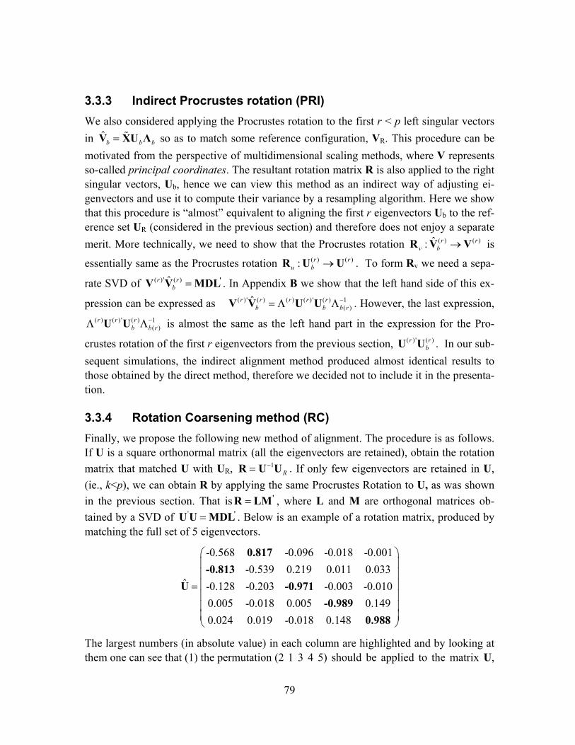
79

3.3.3 Indirect Procrustes rotation (PRI) We also considered applying the Procrustes rotation to the first r < p left singular vectors in ˆ

b b b=V XU Λ% so as to match some reference configuration, VR. This procedure can be motivated from the perspective of multidimensional scaling methods, where V represents so-called principal coordinates. The resultant rotation matrix R is also applied to the right singular vectors, Ub, hence we can view this method as an indirect way of adjusting ei-genvectors and use it to compute their variance by a resampling algorithm. Here we show that this procedure is “almost” equivalent to aligning the first r eigenvectors Ub to the ref-erence set UR (considered in the previous section) and therefore does not enjoy a separate merit. More technically, we need to show that the Procrustes rotation ( ) ( )ˆ: r r

v b →R V V is

essentially same as the Procrustes rotation ( ) ( ): r ru b →R U U . To form Rv we need a sepa-

rate SVD of ( ) ' ( )ˆr rb = 'V V MDL . In Appendix B we show that the left hand side of this ex-

pression can be expressed as ( ) ' ( ) ( ) ( ) ' ( ) 1( )

ˆr r r r rb b b r

−= Λ ΛV V U U . However, the last expression, ( ) ( ) ' ( ) 1

( )r r r

b b r−Λ ΛU U is almost the same as the left hand part in the expression for the Pro-

crustes rotation of the first r eigenvectors from the previous section, ( ) ' ( )r rbU U . In our sub-

sequent simulations, the indirect alignment method produced almost identical results to those obtained by the direct method, therefore we decided not to include it in the presenta-tion.

3.3.4 Rotation Coarsening method (RC) Finally, we propose the following new method of alignment. The procedure is as follows. If U is a square orthonormal matrix (all the eigenvectors are retained), obtain the rotation matrix that matched U with UR, 1

R−=R U U . If only few eigenvectors are retained in U,

(ie., k<p), we can obtain R by applying the same Procrustes Rotation to U, as was shown in the previous section. That is = 'R LM , where L and M are orthogonal matrices ob-tained by a SVD of ' = 'U U MDL . Below is an example of a rotation matrix, produced by matching the full set of 5 eigenvectors.

-0.568 -0.096 -0.018 -0.001-0.539 0.219 0.011 0.033

ˆ -0.128 -0.203 -0.003 -0.0100.005 -0.018 0.005 0.1490.024 0.019 -0.018 0.148

=

0.817-0.813

U -0.971-0.989

0.988

The largest numbers (in absolute value) in each column are highlighted and by looking at them one can see that (1) the permutation (2 1 3 4 5) should be applied to the matrix U,

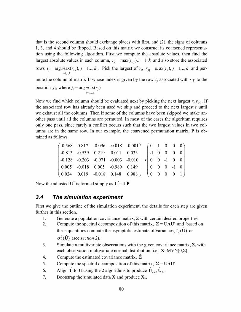
80

that is the second column should exchange places with first, and (2), the signs of columns 1, 3, and 4 should be flipped. Based on this matrix we construct its coarsened representa-tion using the following algorithm. First we compute the absolute values, then find the largest absolute values in each column, ,max( ), 1..j i jr r i k= = and also store the associated

rows ,1,..,

arg ax( ), 1,..,j i ji k

i m r j k=

= = . Pick the largest of rj, [1] ax( ), 1,..,jr m r j k= = and per-

mute the column of matrix U whose index is given by the row 1j

i associated with r[1] to the

position j1, where 11,..,

arg ax( )jj k

j m r=

=

Now we find which column should be evaluated next by picking the next largest r, r[2]. If the associated row has already been used we skip and proceed to the next largest r until we exhaust all the columns. Then if some of the columns have been skipped we make an-other pass until all the columns are permuted. In most of the cases the algorithm requires only one pass, since rarely a conflict occurs such that the two largest values in two col-umns are in the same row. In our example, the coarsened permutation matrix, P is ob-tained as follows

-0.568 0.817 -0.096 -0.018 -0.001 0 1 0 0 0-0.813 -0.539 0.219 0.011 0.033 -1 0 0 0 0-0.128 -0.203 -0.971 -0.003 -0.010 0 0 -1 0 00.005 -0.018 0.005 -0.989 0.149 0 0 0 -1 00.024 0.019 -0.018 0.148 0.988 0 0 0 0 1

→

Now the adjusted U* is formed simply as U*= UP

3.4 The simulation experiment First we give the outline of the simulation experiment, the details for each step are given further in this section.

1. Generate a population covariance matrix, Σ with certain desired properties 2. Compute the spectral decomposition of this matrix, Σ = UΛU' and based on

these quantities compute the asymptotic estimate of variances, ˆ( )AV U or 2 ˆ( )Aσ U (see section 2).

3. Simulate n multivariate observations with the given covariance matrix, Σ, with each observation multivariate normal distribution, i.e. X~MVN(0,Σ).

4. Compute the estimated covariance matrix, Σ 5. Compute the spectral decomposition of this matrix, ˆˆ ˆ ˆΣ = UΛU' 6. Align U to U using the 2 algorithms to produce ˆ ˆ,CL RCU U 7. Bootstrap the simulated data X and produce Xb.

81

8. Compute the estimated bootstrap covariance matrix, ˆbΣ

9. Compute the spectral decomposition of this matrix, 'ˆˆ ˆ ˆb b b bΣ = U Λ U

10. Align the eigenvectors with respect to the aligned empirical eigenvectors, ˆCLU

and produce the doubly aligned eigenvectors using the Clarkson, and Coars-ened Rotation, ˆ ˆ,b b

CL RCU U 11. Repeat steps 7-10, producing B bootstrap samples. 12. Compute bootstrap estimates of standard errors for unaligned (N) and aligned

eigenvectors, ˆ ˆ ˆ ˆ ˆ ˆ( ), ( ), ( )B B BN CL RCV V VU U U .

13. Compute the estimate of the absolute discrepancy between the bootstrap stan-dard errors and those obtained by the asymptotic formula (benchmark),

( ) ( ) ˆ ˆˆ( , ) | ( ) ( ) |i iB AB Aδ σ σ= −U U

14. Repeat steps 3-13 M times and produce a Monte Carlo distribution for the bootstrap estimates of standard errors obtained in step 12.

15. Produce MC summaries (means and standard errors) for the discrepancies computed in step 13.

16. Compute the Monte Carlo estimates ˆ ˆ ˆ ˆ ˆ ˆ( ), ( ), ( )MC MC MCN CL RCV V VU U U of variances

of eigenvectors based on M replications of U and using different alignment schemes

17. Plot the histograms of distribution of bootstrap estimates obtained in step 15 with the benchmarks obtained in steps 2 and 16

Details and comments on the simulation experiment

Step 1:

Fix the population variance-covariance matrix Σ (p by p). This matrix could be of various patterns: general symmetric, block diagonal, or of low rank. In all cases we are specifi-cally interested in the matrices having or not having similar eigenvalues. We can model this situation as 'Σ = UΛU , where U is an n by s orthogonal matrix with s≤p and Λ is a diagonal matrix with the eigenvalues ordered from largest to smallest and setting some of them to be approximately equal. We could perturb the model covariance matrix by a di-agonal matrix ψ to obtain +Σ = FΛF' Ψ (i.e the standard factor analysis model). This would make the eigenstructure of our simulated covariance matrix, Σ , even farther away from the modeled situation which is not desirable, hence we expressed the population co-variance matrix asΣ = FΛF'

Step 2

Compute the associated “population” eigenvalues and eigenvectors, , i iλ u , i =1...p, and compute the asymptotic variances of their sample estimates, as explained in section 2. In our simulation we use p=5 with several covariance patterns. In pattern 1, for example, the eigenvalues are chosen to be uniformly spread out (2.2, 1.4, 0.8, 0.4, 0.3). The eigenvalues

82

sum up to 5 (number of variables), which effectively makes the population covariance ma-trix a correlation matrix. Notice that while the eigenvalues are fixed at desired levels, the population eigenvectors, U, were simulated as arbitrary normalized and orthogonal vec-tors. Compute the asymptotic standard errors for the elements of the U matrix, ˆ( )AV U .

Step 3

Simulate n rows of matrix X as multivariate normal x ~MVN(0,Σ). This is accomplished via the Cholesky decomposition of the population covariance matrix, C=Chol(Σ) such that C is upper triangular and 'CC = Σ . Then we can set X=ZC, where z~MVN(0,I) (see Thisted (1988).

Steps 4-6

Estimate the sample covariance matrix Σ and compute the eigenvectors ˆ iu and eigenval-

ues iλ , i =1..p. These eigenvectors will serve as “population eigenvectors” for the boot-strap procedure to produce their variance estimates. Since we will be aggregating and comparing bootstrap variance estimates across simulated ˆ iu , the later need to be aligned with respect to the true population eigenvectors u (we use the Clarkson procedure to do that).

Steps 7-13

Bootstrap the data in X and produce B=1000 (say) bootstrap samples Xb. Compute the bootstrapped estimates of the variances and covariances for the eigenvectors using expres-sion (3.2) :

Denote the square roots of these estimates, ( ) ˆˆ ( )iBσ U . The bootstrap estimates can be of the

following three forms a. Unaligned bootstrapped eigenvectors data (referred to as N) b. Aligned using CL algorithm (Clarkson algorithm) c. Aligned using our RC, coarsened rotation method

For each estimate obtained in a-d we compute the absolute difference between this esti-mate and the asymptotic estimate as

( ) ( ) ˆ ˆˆ( , ) | ( ) ( ) |i iB AB Aδ σ σ= −U U (3.5)

Steps 14- 15

Repeat steps 3 through 13 with the number of iterations, M=1000 for each of the 3 eigen-value structures (patterns). Compute the Monte Carlo estimates of standard errors for the bootstrap estimates ˆˆ ( )Bσ U as

83

2 1 ( ) (.) 2

1

ˆ ˆ ˆ ˆ( ) ( 1) ( )M

iMC B B B

iMσ σ σ σ−

=

= − −∑ ,

where (.) 1 ( )

1

ˆ ˆM

iB B

iMσ σ−

=

= ∑ , is the average of bootstrap estimates.

Compute the Monte Carlo estimates of standard errors and expected value of ( )ˆ ( , )i B Aδ (defined in the expression (3.5)):

2 (.) 1 ( ) (.) 2

1

ˆ ˆ ˆˆ ( ( , )) { ( 1)} ( ( , ) ( , ))M

iMC

iB A M M B A B Aσ δ δ δ−

=

= − −∑ (3.6)

where ( ) 1 ( )

1

ˆ ˆ( , ) ( , )M

i

iB A M B Aδ δ−

=

= ∑. is the Monte Carlo estimate of the expected value of

( )ˆ ( , )i B Aδ . It allows us to evaluate how close is the match between the bootstrap estimates of standard error and the benchmark estimate. Compute the Monte Carlo estimates of standard errors for the bootstrap estimates of the differences between the absolute differ-ences against the benchmark for various bootstrap methods,

( ) ( ) ( )ˆ ( , ) ( , ) ( , )i i iRC CLe RC CL B A B Aδ δ= − , and also e(RC,N), and e(CL,N) which are de-

fined similarly. Compute the Monte Carlo estimate of the standard error associated with these quantities

2 ( ) 1 ( ) (.) 2

1

ˆ ˆ ˆ ˆ( ( , )) ( ( 1)) ( ( , ) ( , ))M

iMC RC CL RC CL RC CL

ie B B M M e B B e B Bσ −

=

= − −∑. ,

where, (.) 1 ( )

1

ˆ ˆ( , ) ( , )M

iRC CL RC CL

ie B B M e B B−

=

= ∑

Steps 16-17

Besides providing information about the distribution of bootstrap variance estimates, we can utilize the M Monte Carlo simulations to compute the Monte Carlo estimates of vari-ance, each of them depend on a particular alignment scheme. For example, for Clarkson method

( )( )'MC ( ) ( ) ( ) ( ) ( ) ( )CL

1 1

1 1ˆ ˆ ˆ ˆ ˆ ˆ ˆ, 1

M Mi i i

CL CL CL CL CL CLi iM M= =

= =− ∑ ∑. . .V U - U U - U U U (3.7)

The standard errors are the square roots of the diagonal elements of MCV .

This provides another set of benchmarks to be compared with the bootstrap variance. We can also use Monte Carlo estimates to verify the asymptotic formulas and also provide partial evidence about the efficiency of different alignment schemes. Of course, the fact

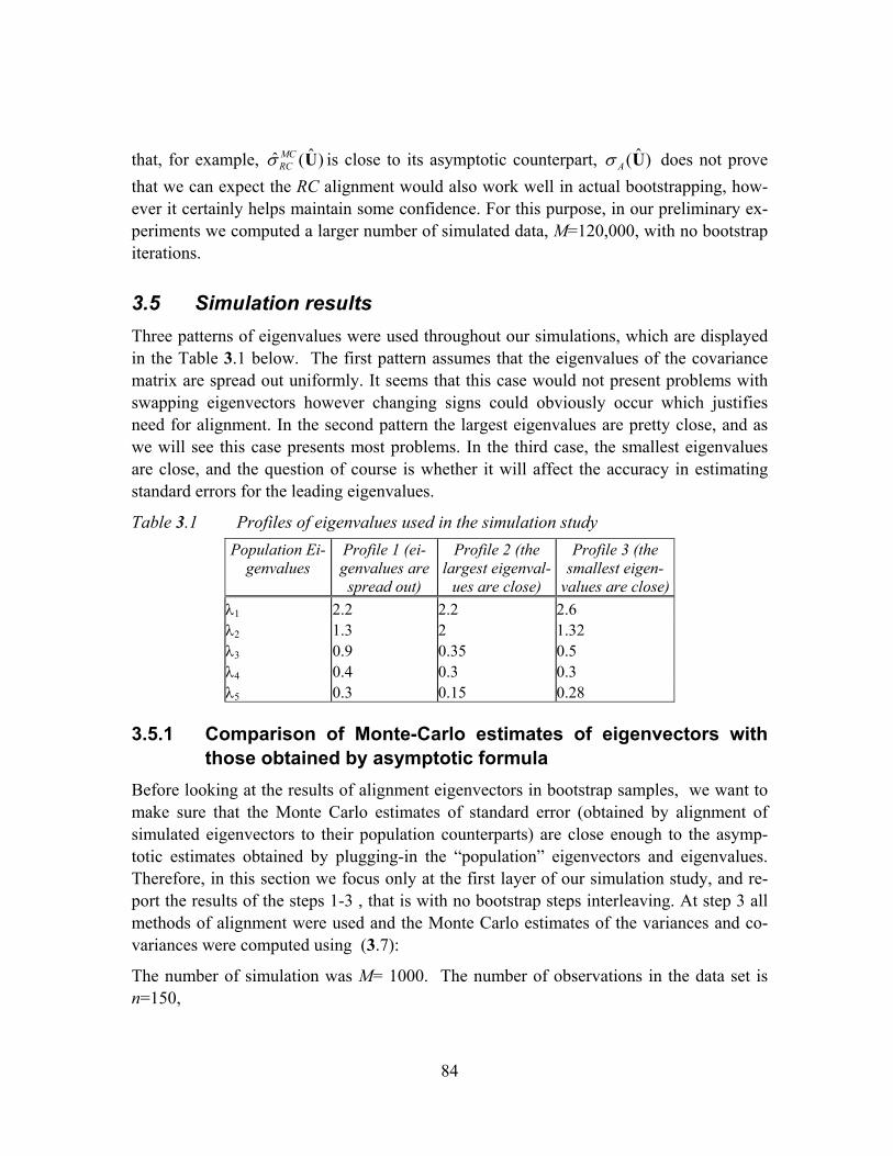
84

that, for example, ˆˆ ( )MCRCσ U is close to its asymptotic counterpart, ˆ( )Aσ U does not prove

that we can expect the RC alignment would also work well in actual bootstrapping, how-ever it certainly helps maintain some confidence. For this purpose, in our preliminary ex-periments we computed a larger number of simulated data, M=120,000, with no bootstrap iterations.

3.5 Simulation results Three patterns of eigenvalues were used throughout our simulations, which are displayed in the Table 3.1 below. The first pattern assumes that the eigenvalues of the covariance matrix are spread out uniformly. It seems that this case would not present problems with swapping eigenvectors however changing signs could obviously occur which justifies need for alignment. In the second pattern the largest eigenvalues are pretty close, and as we will see this case presents most problems. In the third case, the smallest eigenvalues are close, and the question of course is whether it will affect the accuracy in estimating standard errors for the leading eigenvalues.

Table 3.1 Profiles of eigenvalues used in the simulation study Population Ei-

genvalues Profile 1 (ei-genvalues are spread out)

Profile 2 (the largest eigenval-

ues are close)

Profile 3 (the smallest eigen-

values are close) λ1 2.2 2.2 2.6 λ2 1.3 2 1.32 λ3 0.9 0.35 0.5 λ4 0.4 0.3 0.3 λ5 0.3 0.15 0.28

3.5.1 Comparison of Monte-Carlo estimates of eigenvectors with those obtained by asymptotic formula

Before looking at the results of alignment eigenvectors in bootstrap samples, we want to make sure that the Monte Carlo estimates of standard error (obtained by alignment of simulated eigenvectors to their population counterparts) are close enough to the asymp-totic estimates obtained by plugging-in the “population” eigenvectors and eigenvalues. Therefore, in this section we focus only at the first layer of our simulation study, and re-port the results of the steps 1-3 , that is with no bootstrap steps interleaving. At step 3 all methods of alignment were used and the Monte Carlo estimates of the variances and co-variances were computed using (3.7):

The number of simulation was M= 1000. The number of observations in the data set is n=150,

85

Several results were obtained for different patterns of eigenvalues. In the tables below, each column corresponds to the element eij for the i-th element of eigenvector j. Only three first eigenvectors are reported. All values are multiplied by 1000. The results for each profile are reported in a separate table.

Profile 1 (Eigenvalues are uniformly distributed)

First compare the average simulated eigenvectors under no alignment and when alignment is applied to the true population eigenvectors. We can see that the when eigenvectors are not aligned, flipping of signs causes significant shrinking of their values to zero. For ex-ample, for the first profile the signs were switched for at least one column in 2.5% of simulations, which of course inflates the standard estimates considerably.

Table 3.2 Means and standard errors of simulated eigenvectors (Profile 1, using first 3 eigenvectors)

Population eigenvectors Unaligned eigenvectors Clarkson method Coarsened Rotation

Actual values Mean values for 1000 iterations of MC simulation

e1 e2 e3 e1 e2 e3 e1 e2 e3 e1 e2 e3

703.99 -557.93 139.44 -0.07 -3.59 6.03 693.20 -539.11 133.29 693.20 -539.11 133.29

-137.96 36.57 890.26 -2.44 -2.68 32.27 -133.34 33.95 862.97 -133.34 33.95 862.97

170.71 -251.54 -327.39 -0.16 1.29 -16.29 165.21 -244.22 -320.35 165.21 -244.22 -320.35

-105.59 337.82 -273.53 1.58 2.58 -14.52 -103.56 326.69 -266.32 -103.56 326.69 -266.32

667.14 714.13 77.43 1.40 -2.48 7.61 654.73 690.20 73.68 654.73 690.20 73.68

Asymptotic estimates of standard errors Monte Carlo Estimate of Standard Error based on 1000 iterations

87.53 112.57 113.02 699.31 552.93 175.75 91.67 117.75 117.08 91.67 117.75 117.08

71.49 152.37 50.97 150.83 165.79 864.76 70.62 162.29 58.07 70.62 162.29 58.07

59.27 83.03 108.71 177.23 257.98 339.61 63.45 86.21 111.14 63.45 86.21 111.14

64.67 67.99 95.92 123.43 335.87 282.48 66.64 73.97 97.85 66.64 73.97 97.85

109.95 103.66 130.63 665.25 698.85 159.87 114.81 111.42 139.97 114.81 111.42 139.97

The asymptotic estimates agree very well with both the Clarkson method and the Coars-ened Rotation method while the estimates obtained with the unaligned eigenvectors are, as should be expected, substantially overestimated. In fact our method of coarsened rotation produced exactly same results as the Clarkson method, which suggests that it can be used in situations when applying Clarkson method is unfeasible.

Profile 2 (The largest eigenvalues are close)

86

In this case, the largest eigenvalues are taken to be close to each other. Surprisingly, the asymptotic formula does not agree very well with the estimates obtained with any of the methods. However, by looking at the averages of the eigenvectors obtained over the Monte Carlo samples, we can see that rotations do make them closer to their population counterparts. Probably the asymptotic formula does not work well for the cases when the leading eigenvalues are close and it tends to produce greatly inflated estimates of standard error. On the other hand, it appears that the performance of the alignment procedures is much poorer when eigenvectors tend to swap too often. Even small number of incorrect assignment, though may not shift the averages too far from their population counterparts, could affect the estimated variances badly. What happens when the ties occur with the smallest eigenvalues? This is shown in the case of Profile 3.

Table 3.3 Means and standard errors of the simulated eigenvectors (Profile 2, using first 3 eigenvectors)


Method


e1 e2 e3 e1 e2 e3 e1 e2 e3 e1 e2 e3

-109.88 413.93 713.10 -4.05 -9.64 23.25 -102.85 377.05 656.33 -102.85 377.05 655.82

-360.06 -108.42 -540.33 -1.68 -4.02 -8.39 -328.20 -102.63 -495.62 -328.20 -102.63 -495.90

-444.26 355.68 43.61 -3.97 -13.11 -1.12 -406.32 320.25 31.78 -406.32 320.25 32.93

456.61 -553.15 287.47 4.70 18.65 8.48 421.84 -498.33 259.69 421.84 -498.33 260.26

672.62 620.01 -339.10 2.67 1.79 -8.52 606.24 569.83 -314.56 606.24 569.83 -314.46


355.93 100.19 218.21 254.56 348.45 654.81 169.46 68.63 166.97 169.46 68.63 167.26

97.11 309.83 187.17 304.44 225.44 504.27 60.42 146.68 147.83 60.42 146.68 147.39

305.88 381.61 416.63 418.90 385.35 370.30 150.25 183.48 291.54 150.25 183.48 291.68

474.12 391.61 182.22 490.54 522.28 295.88 226.38 189.28 136.45 226.38 189.28 136.50

531.14 576.20 50.29 653.72 637.85 304.17 255.17 275.98 54.79 255.17 275.98 55.02

Profile 3 (The smallest eigenvalues are close)

In this case, the standard errors of the eigenvectors obtained by either method of align-ment are close to that obtained by the asymptotic formula, at least for the first three col-umns associated with the largest eigenvalues. This means that swapping of the eigenvec-tors associated with smallest eigenvalues does not prevent correct alignment of the leading eigenvectors.

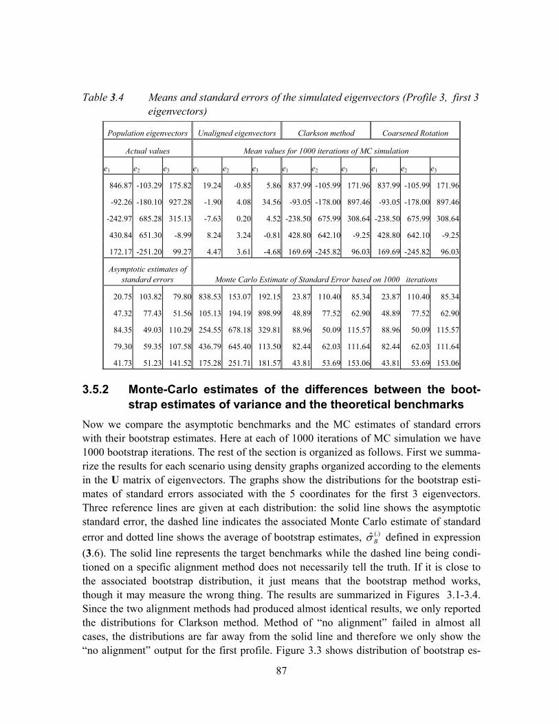
87

Table 3.4 Means and standard errors of the simulated eigenvectors (Profile 3, first 3 eigenvectors)



e1 e2 e3 e1 e2 e3 e1 e2 e3 e1 e2 e3

846.87 -103.29 175.82 19.24 -0.85 5.86 837.99 -105.99 171.96 837.99 -105.99 171.96

-92.26 -180.10 927.28 -1.90 4.08 34.56 -93.05 -178.00 897.46 -93.05 -178.00 897.46

-242.97 685.28 315.13 -7.63 0.20 4.52 -238.50 675.99 308.64 -238.50 675.99 308.64

430.84 651.30 -8.99 8.24 3.24 -0.81 428.80 642.10 -9.25 428.80 642.10 -9.25

172.17 -251.20 99.27 4.47 3.61 -4.68 169.69 -245.82 96.03 169.69 -245.82 96.03


20.75 103.82 79.80 838.53 153.07 192.15 23.87 110.40 85.34 23.87 110.40 85.34

47.32 77.43 51.56 105.13 194.19 898.99 48.89 77.52 62.90 48.89 77.52 62.90

84.35 49.03 110.29 254.55 678.18 329.81 88.96 50.09 115.57 88.96 50.09 115.57

79.30 59.35 107.58 436.79 645.40 113.50 82.44 62.03 111.64 82.44 62.03 111.64

41.73 51.23 141.52 175.28 251.71 181.57 43.81 53.69 153.06 43.81 53.69 153.06

3.5.2 Monte-Carlo estimates of the differences between the boot-strap estimates of variance and the theoretical benchmarks

Now we compare the asymptotic benchmarks and the MC estimates of standard errors with their bootstrap estimates. Here at each of 1000 iterations of MC simulation we have 1000 bootstrap iterations. The rest of the section is organized as follows. First we summa-rize the results for each scenario using density graphs organized according to the elements in the U matrix of eigenvectors. The graphs show the distributions for the bootstrap esti-mates of standard errors associated with the 5 coordinates for the first 3 eigenvectors. Three reference lines are given at each distribution: the solid line shows the asymptotic standard error, the dashed line indicates the associated Monte Carlo estimate of standard error and dotted line shows the average of bootstrap estimates, (.)ˆBσ defined in expression (3.6). The solid line represents the target benchmarks while the dashed line being condi-tioned on a specific alignment method does not necessarily tell the truth. If it is close to the associated bootstrap distribution, it just means that the bootstrap method works, though it may measure the wrong thing. The results are summarized in Figures 3.1-3.4. Since the two alignment methods had produced almost identical results, we only reported the distributions for Clarkson method. Method of “no alignment” failed in almost all cases, the distributions are far away from the solid line and therefore we only show the “no alignment” output for the first profile. Figure 3.3 shows distribution of bootstrap es-

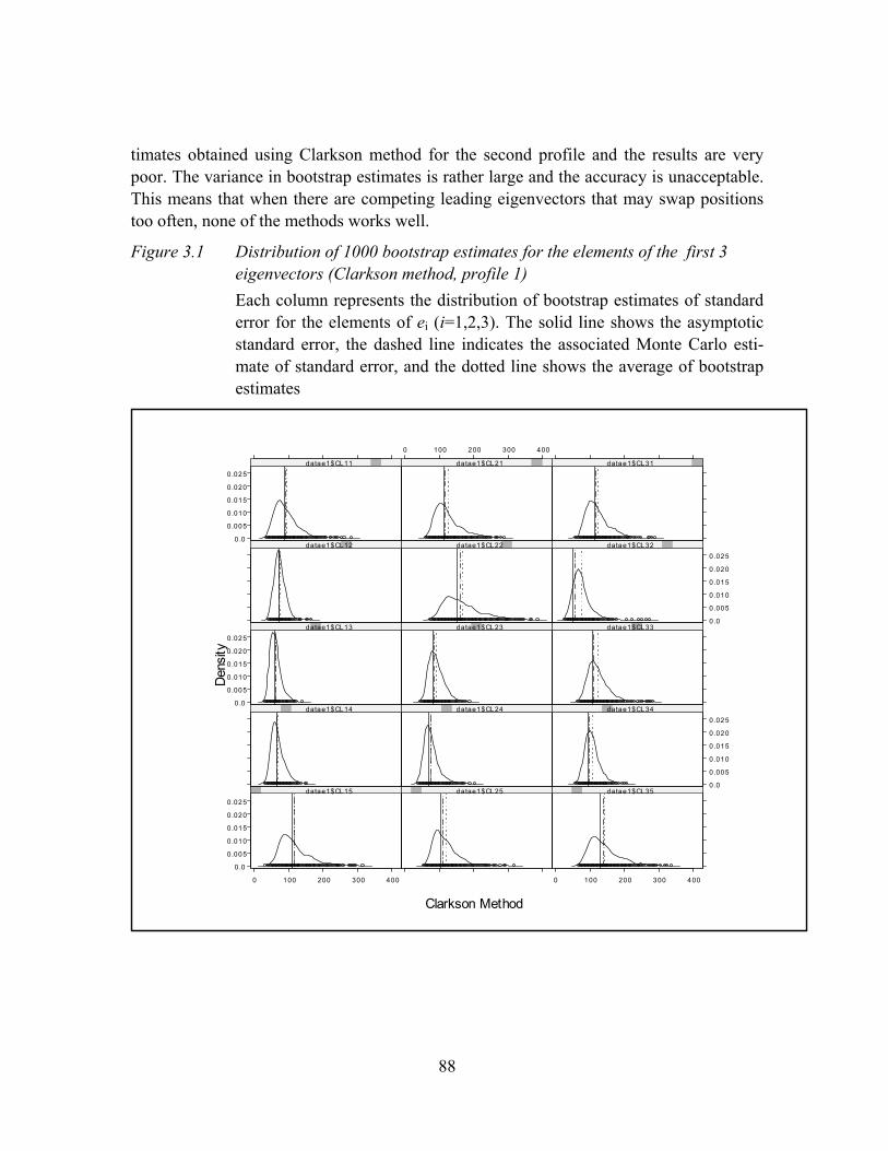
88

timates obtained using Clarkson method for the second profile and the results are very poor. The variance in bootstrap estimates is rather large and the accuracy is unacceptable. This means that when there are competing leading eigenvectors that may swap positions too often, none of the methods works well.

Figure 3.1 Distribution of 1000 bootstrap estimates for the elements of the first 3 eigenvectors (Clarkson method, profile 1) Each column represents the distribution of bootstrap estimates of standard error for the elements of ei (i=1,2,3). The solid line shows the asymptotic standard error, the dashed line indicates the associated Monte Carlo esti-mate of standard error, and the dotted line shows the average of bootstrap estimates

0.0

0.005

0.010

0.015

0.020

0.025datae1$CL15

0 100 200 300 400

datae1$CL25 datae1$CL35

0 100 200 300 400


0.0

0.005

0.010

0.015

0.020

0.025datae1$CL34

0.0

0.005

0.010

0.015

0.020

0.025datae1$CL13 datae1$CL23 datae1$CL33


0.0

0.005

0.010

0.015

0.020

0.025datae1$CL32

0.0

0.005

0.010

0.015

0.020

0.025datae1$CL11 datae1$CL21

0 100 200 300 400

datae1$CL31

Clarkson Method

Den

sity

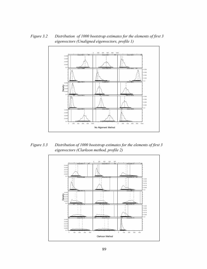
89

Figure 3.2 Distribution of 1000 bootstrap estimates for the elements of first 3 eigenvectors (Unaligned eigenvectors, profile 1)

0.0

0.002

0.004

0.006

0.008datae1$N15

0 200 400 600 800 1000

datae1$N25 datae1$N35

0 200 400 600 800 1000


0.0

0.002

0.004

0.006

0.008datae1$N34

0.0

0.002

0.004

0.006

0.008datae1$N13 datae1$N23 datae1$N33


0.0

0.002

0.004

0.006

0.008datae1$N32

0.0

0.002

0.004

0.006

0.008datae1$N11 datae1$N21

0 200 400 600 800 1000

datae1$N31

No Alignment Method

Dens

ity

Figure 3.3 Distribution of 1000 bootstrap estimates for the elements of first 3 eigenvectors (Clarkson method, profile 2)

0.0

0.005

0.010

0.015

0.020

0.025datae2$CL15

0 100 200 300 400


0 100 200 300 400


0.0

0.005

0.010

0.015

0.020

0.025datae2$CL34

0.0

0.005

0.010

0.015

0.020

0.025datae2$CL13 datae2$CL23 datae2$CL33


0.0

0.005

0.010

0.015

0.020

0.025datae2$CL32

0.0

0.005

0.010

0.015

0.020

0.025datae2$CL11 datae2$CL21

0 100 200 300 400

datae2$CL31

Clarkson Method

Dens

ity

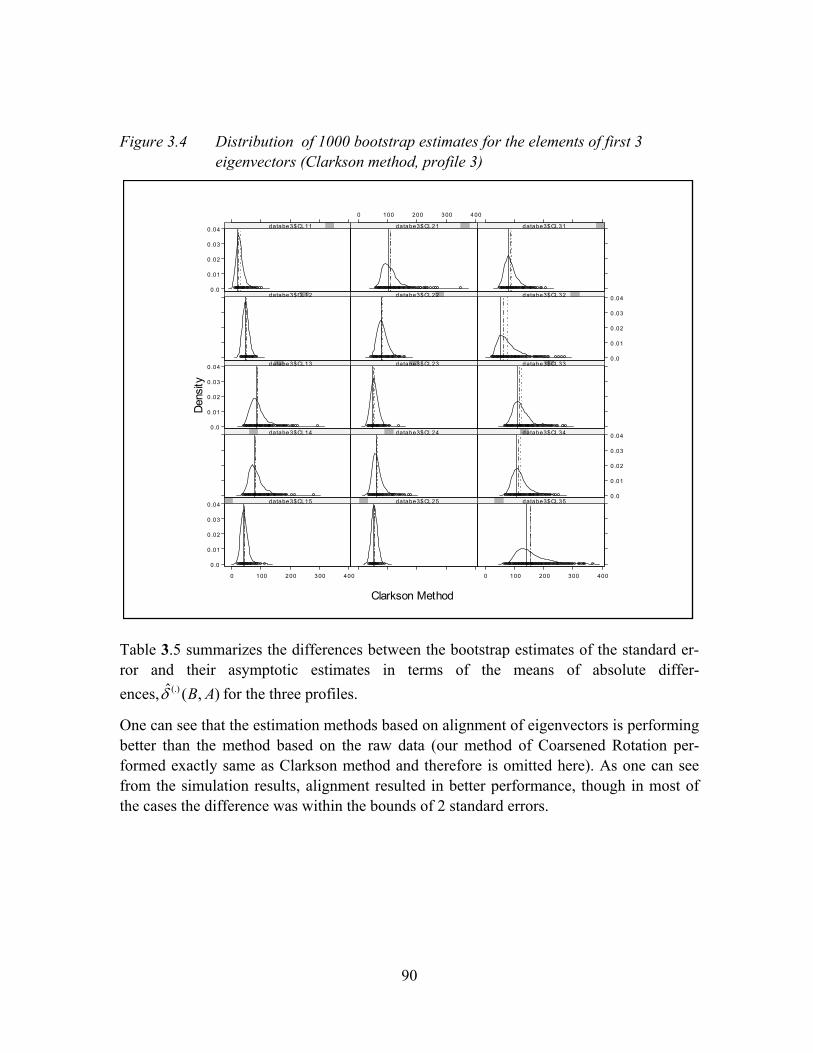
90

Figure 3.4 Distribution of 1000 bootstrap estimates for the elements of first 3 eigenvectors (Clarkson method, profile 3)

0.0

0 .01

0.02

0.03

0.04 databe3$CL15

0 100 200 300 400

databe3$CL25 databe3$CL35

0 100 200 300 400


0.0

0 .01

0.02

0.03

0.04databe3$CL340.0

0 .01

0.02

0.03

0.04 databe3$CL13 databe3$CL23 databe3$CL33


0.0

0 .01

0.02

0.03

0.04databe3$CL320.0

0 .01

0.02

0.03

0.04 databe3$CL11 databe3$CL21

0 100 200 300 400

databe3$CL31

Clarkson Method

Dens

ity

Table 3.5 summarizes the differences between the bootstrap estimates of the standard er-ror and their asymptotic estimates in terms of the means of absolute differ-ences, (.)ˆ ( , )B Aδ for the three profiles.

One can see that the estimation methods based on alignment of eigenvectors is performing better than the method based on the raw data (our method of Coarsened Rotation per-formed exactly same as Clarkson method and therefore is omitted here). As one can see from the simulation results, alignment resulted in better performance, though in most of the cases the difference was within the bounds of 2 standard errors.

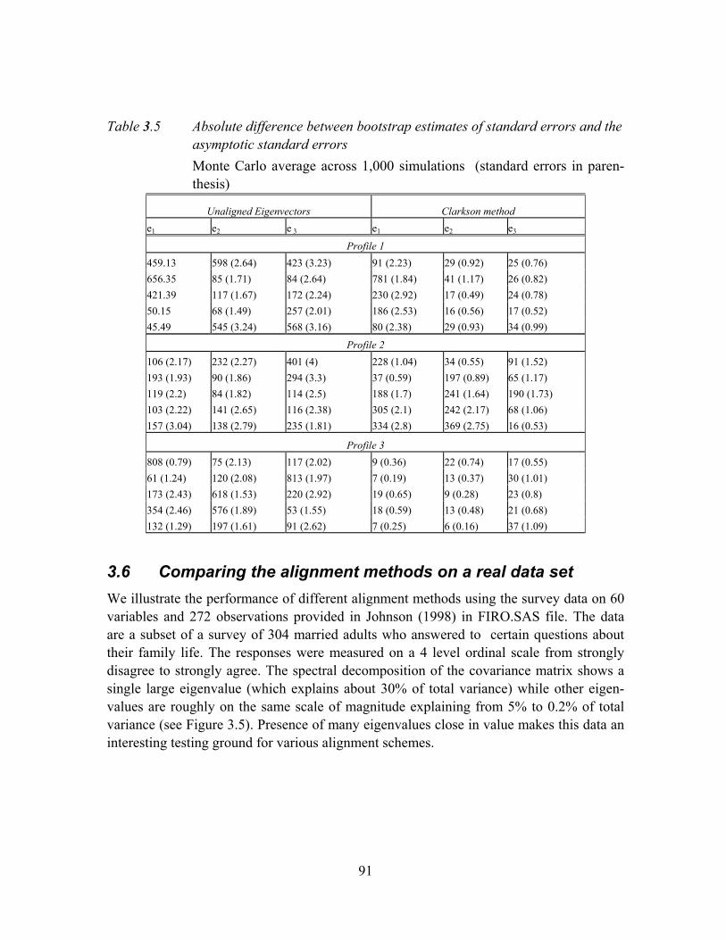
91

Table 3.5 Absolute difference between bootstrap estimates of standard errors and the asymptotic standard errors Monte Carlo average across 1,000 simulations (standard errors in paren-thesis)

Unaligned Eigenvectors Clarkson method e1 e2 e 3 e1 e2 e3

Profile 1 459.13 598 (2.64) 423 (3.23) 91 (2.23) 29 (0.92) 25 (0.76) 656.35 85 (1.71) 84 (2.64) 781 (1.84) 41 (1.17) 26 (0.82) 421.39 117 (1.67) 172 (2.24) 230 (2.92) 17 (0.49) 24 (0.78) 50.15 68 (1.49) 257 (2.01) 186 (2.53) 16 (0.56) 17 (0.52) 45.49 545 (3.24) 568 (3.16) 80 (2.38) 29 (0.93) 34 (0.99)

Profile 2 106 (2.17) 232 (2.27) 401 (4) 228 (1.04) 34 (0.55) 91 (1.52) 193 (1.93) 90 (1.86) 294 (3.3) 37 (0.59) 197 (0.89) 65 (1.17) 119 (2.2) 84 (1.82) 114 (2.5) 188 (1.7) 241 (1.64) 190 (1.73) 103 (2.22) 141 (2.65) 116 (2.38) 305 (2.1) 242 (2.17) 68 (1.06) 157 (3.04) 138 (2.79) 235 (1.81) 334 (2.8) 369 (2.75) 16 (0.53)

Profile 3 808 (0.79) 75 (2.13) 117 (2.02) 9 (0.36) 22 (0.74) 17 (0.55) 61 (1.24) 120 (2.08) 813 (1.97) 7 (0.19) 13 (0.37) 30 (1.01) 173 (2.43) 618 (1.53) 220 (2.92) 19 (0.65) 9 (0.28) 23 (0.8) 354 (2.46) 576 (1.89) 53 (1.55) 18 (0.59) 13 (0.48) 21 (0.68) 132 (1.29) 197 (1.61) 91 (2.62) 7 (0.25) 6 (0.16) 37 (1.09)

3.6 Comparing the alignment methods on a real data set We illustrate the performance of different alignment methods using the survey data on 60 variables and 272 observations provided in Johnson (1998) in FIRO.SAS file. The data are a subset of a survey of 304 married adults who answered to certain questions about their family life. The responses were measured on a 4 level ordinal scale from strongly disagree to strongly agree. The spectral decomposition of the covariance matrix shows a single large eigenvalue (which explains about 30% of total variance) while other eigen-values are roughly on the same scale of magnitude explaining from 5% to 0.2% of total variance (see Figure 3.5). Presence of many eigenvalues close in value makes this data an interesting testing ground for various alignment schemes.

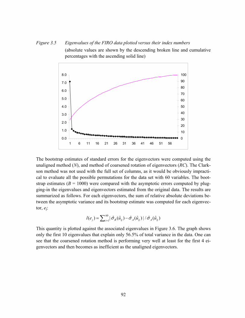
92

Figure 3.5 Eigenvalues of the FIRO data plotted versus their index numbers (absolute values are shown by the descending broken line and cumulative percentages with the ascending solid line)

0.0

1.0

2.0

3.0

4.0

5.0

6.0

7.0

8.0

1 6 11 16 21 26 31 36 41 46 51 560

10

20

30

40

50

60

70

80

90

100

The bootstrap estimates of standard errors for the eigenvectors were computed using the unaligned method (N), and method of coarsened rotation of eigenvectors (RC). The Clark-son method was not used with the full set of columns, as it would be obviously impracti-cal to evaluate all the possible permutations for the data set with 60 variables. The boot-strap estimates (B = 1000) were compared with the asymptotic errors computed by plug-ging-in the eigenvalues and eigenvectors estimated from the original data. The results are summarized as follows. For each eigenvectors, the sum of relative absolute deviations be-tween the asymptotic variance and its bootstrap estimate was computed for each eigenvec-tor, ej:

60

1ˆ ˆ ˆ ˆ ˆ ˆ( ) | ( ) ( ) | / ( )j B ij A ij A iji

l e u u uσ σ σ=

= −∑

This quantity is plotted against the associated eigenvalues in Figure 3.6. The graph shows only the first 10 eigenvalues that explain only 56.5% of total variance in the data. One can see that the coarsened rotation method is performing very well at least for the first 4 ei-genvectors and then becomes as inefficient as the unaligned eigenvectors.

93

Figure 3.6 Relative discrepancy between bootstrap and asymptotic estimates, l(ej), for the unaligned and aligned eigenvectors (along the horizontal axes are the eigenvalues, all 60 eigenvectors were used)

0123456789

10

0 2 4 6 8

Unaligned eigenvectors Coarsened Rotation

To understand why the alignment breaks down after 4th eigenvector, we computed the proportion of times each eigenvector swapped position with other eigenvector (according to our coarsened rotation algorithm). For those cases when no swap has occurred we com-puted proportion of times the sign flipped. First we can observe that the first eigenvector never swaps, which should be expected given that it is so much larger than the other. The change of sign normally occurs in about half of the cases, which also should be expected since a priory it seems reasonable that the assignment of signs is a Bernoulli random vari-ate with p=0.5. Surprisingly, alignment works well even for the fourth eigenvector, that is under 47% of swaps! After the number of swaps increases 50%, aligning becomes inef-ficient.

To add the Clarkson method to the picture we performed another 1000 bootstrap iterations only with alignment of the first 5 eigenvectors of the covariance matrix. The results are shown in Figure 3.7, along the horizontal axes are the eigenvalues. Notice that since only 5 of 60 eigenvectors were retained, we also used the method of Procrustes rotation di-rectly on the eigenvectors in U. The coarsened rotation is almost identical to Clarkson’s method and (shown with filled circles inside squares) is outperforming the unrotated solu-tion, at least for the first 4 eigenvectors.

94

Table 3.6 Proportion of swaps and sign changes in the first 10 eigenvectors

Eigenvector index

Proportion of swaps

Proportion of sign changes (when no

swaps occur) 1 0.00 0.552 0.18 0.533 0.34 0.524 0.47 0.525 0.67 0.516 0.71 0.477 0.76 0.498 0.78 0.539 0.81 0.52

10 0.86 0.55

Figure 3.7 Relative discrepancy between bootstrap and asymptotic estimates (three methods of alignment versus unaligned eigenvectors)

0

1

2

3

4

5

6

7

8

9

10

0 2 4 6 8

Unaligned eigenvectorsCoarsened Rotation Direct ProcrustesClarkson method

To provide some additional insight, Figures 3.8 shows the bootstrap standard errors for the individual elements of the first eigenvector computed from unaligned eigenvectors and using methods of coarsened and direct Procrustes alignment, plotted against the corre-sponding asymptotic standard error. A similar graph without the unaligned estimates but including Clarkson method is shown in Figure 3.9. The dotted line is y=x.

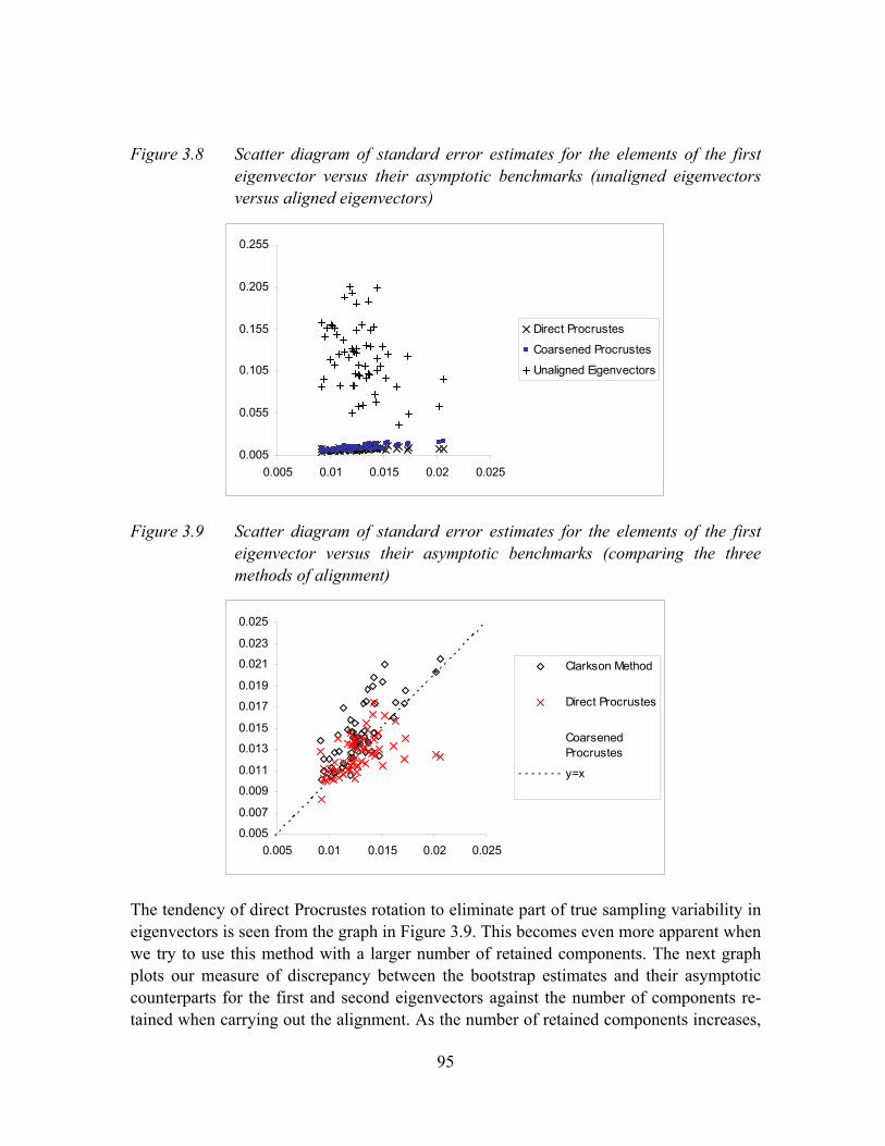
95

Figure 3.8 Scatter diagram of standard error estimates for the elements of the first eigenvector versus their asymptotic benchmarks (unaligned eigenvectors versus aligned eigenvectors)

0.005

0.055

0.105

0.155

0.205

0.255

0.005 0.01 0.015 0.02 0.025

Direct Procrustes

Coarsened Procrustes

Unaligned Eigenvectors

Figure 3.9 Scatter diagram of standard error estimates for the elements of the first eigenvector versus their asymptotic benchmarks (comparing the three methods of alignment)

0.005

0.007

0.009

0.011

0.013

0.015

0.017

0.019

0.021

0.023

0.025

0.005 0.01 0.015 0.02 0.025

Clarkson Method

Direct Procrustes

CoarsenedProcrustes

y=x

The tendency of direct Procrustes rotation to eliminate part of true sampling variability in eigenvectors is seen from the graph in Figure 3.9. This becomes even more apparent when we try to use this method with a larger number of retained components. The next graph plots our measure of discrepancy between the bootstrap estimates and their asymptotic counterparts for the first and second eigenvectors against the number of components re-tained when carrying out the alignment. As the number of retained components increases,

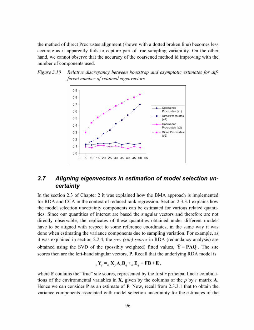
96

the method of direct Procrustes alignment (shown with a dotted broken line) becomes less accurate as it apparently fails to capture part of true sampling variability. On the other hand, we cannot observe that the accuracy of the coarsened method id improving with the number of components used.

Figure 3.10 Relative discrepancy between bootstrap and asymptotic estimates for dif-ferent number of retained eigenvectors

0.0

0.1

0.2

0.3

0.4

0.5

0.6

0.7

0.8

0.9

0 5 10 15 20 25 30 35 40 45 50 55

CoarsenedProcrustes (e1)Direct Procrustes(e1)CoarsenedProcrustes (e2)

Direct Procrustes(e2)

3.7 Aligning eigenvectors in estimation of model selection un-certainty

In the section 2.3 of Chapter 2 it was explained how the BMA approach is implemented for RDA and CCA in the context of reduced rank regression. Section 2.3.3.1 explains how the model selection uncertainty components can be estimated for various related quanti-ties. Since our quantities of interest are based the singular vectors and therefore are not directly observable, the replicates of these quantities obtained under different models have to be aligned with respect to some reference coordinates, in the same way it was done when estimating the variance components due to sampling variation. For example, as it was explained in section 2.2.4, the row (site) scores in RDA (redundancy analysis) are obtained using the SVD of the (possibly weighted) fitted values, 'ˆ =Y PΛQ . The site scores then are the left-hand singular vectors, P. Recall that the underlying RDA model is

n q n p r q n q =Y = X A B + E FB + E ,

where F contains the “true” site scores, represented by the first r principal linear combina-tions of the environmental variables in X, given by the columns of the p by r matrix A. Hence we can consider P as an estimate of F. Now, recall from 2.3.3.1 that to obtain the variance components associated with model selection uncertainty for the estimates of the

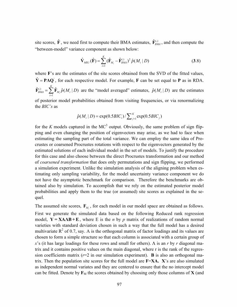
97

site scores, F , we need first to compute their BMA estimates, ( )ˆBMA

.F , and then compute the “between-model” variance component as shown below:

(.) 2

1

ˆ ˆ ˆ ˆ ˆ( ) ( ) ( | )i

K

MSU M BMA ii

p M D=

= −∑V F F F (3.8)

where F’s are the estimates of the site scores obtained from the SVD of the fitted values, 'ˆ =Y PΛQ , for each respective model. For example, F can be set equal to P as in RDA.

(.)

1

ˆ ˆ ˆ ( | )i

K

BMA M ii

p M D=

=∑F F are the “model averaged” estimates, ˆ ( | )ip M D are the estimates

of posterior model probabilities obtained from visiting frequencies, or via renormalizing the BIC’s as

1ˆ ( | ) exp(0.5 ) / exp(0.5 )K

i i jjp M D BIC BIC

== ∑

for the K models captured in the MC3 output. Obviously, the same problem of sign flip-ping and even changing the position of eigenvectors may arise, as we had to face when estimating the sampling part of the total variance. We can employ the same idea of Pro-crustes or coarsened Procrustes rotations with respect to the eigenvectors generated by the estimated solutions of each individual model in the set of models. To justify the procedure for this case and also choose between the direct Procrustes transformation and our method of coarsened transformation that does only permutations and sign flipping, we performed a simulation experiment. Unlike the simulation analysis of the aligning problem when es-timating only sampling variability, for the model uncertainty variance component we do not have the asymptotic benchmark for comparison. Therefore the benchmarks are ob-tained also by simulation. To accomplish that we rely on the estimated posterior model probabilities and apply them to the true (or assumed) site scores as explained in the se-quel.

The assumed site scores, iMF , for each model in our model space are obtained as follows.

First we generate the simulated data based on the following Reduced rank regression model, Y = XAΛB + E , where E is the n by p matrix of realizations of random normal varieties with standard deviation chosen in such a way that the full model has a desired multivariate R2 of 0.7, say. A is the orthogonal matrix of factor loadings and its values are chosen to form a simple structure so that each column is associated with a certain group of x’s (it has large loadings for these rows and small for others). Λ is an r by r diagonal ma-trix and it contains positive values on the main diagonal, where r is the rank of the regres-sion coefficients matrix (r=2 in our simulation experiment). B is also an orthogonal ma-trix. Then the population site scores for the full model are F=XA. X’s are also simulated as independent normal variates and they are centered to ensure that the no intercept model can be fitted. Denote by FM the scores obtained by choosing only those columns of X (and

98

rows of A) that correspond to a given model M. FM=XMAM. This allows us to estimate our benchmark for the variance of model selection simply by using

iMF instead of in formula (3.8) that is,

( ) 2

1

ˆ ˆ( ) ( ) ( | )i

K

MSU M BMA ii

p M D=

= −∑ .V F F F (3.9)

Notice that we use the same estimates of model posterior probabilities as for the estimates based on the site scores obtained from the fitted values. The benchmark is compared to the estimates produced by using the formula (3.8) with the site scores aligned with respect to the reference scores using the direct Procrustes method and the coarsened Procrustes transformation.

The results of a small simulation study are displayed in the graphs below. For each itera-tion of the MC simulation, a “population” reduced rank regression of rank r=4 was con-structed. The number of observations was taken to be n=300, the number of responses (y’s) = 5 and the number of x’s, m = 40. The population factor loadings, A, were con-structed according to the principle of simple structure, that is each factor is associated with some set of x’s and the sets of x’s associated with different factors do not overlap. At each iteration, the multivariate data set (y’s) was generated adding normal errors, Y = FΛB + E . The matrix of singular values, Λ, is diagonal and the singular values are decreasing as powers of 2 i.e. 1, 0.5, 0.025,…. To obtain the set of models and model weights, 20,000 iterations of MC3 procedure for the RRR with rank r=4 was applied within each iteration of Monte Carlo simulation. The first graph (shown in Figure 3.11) shows the simulation protocol for the first 25 Monte Carlo iterations. The points represent the absolute mean deviations (l) of estimated standard errors from the benchmark values computed using formula (3.9) under different alignment schemes for the elements of the first vector in matrix F. That is,

11 1 11

ˆˆ ˆ( ) | ( ) ( ) |nmsu i msu ii

l n V f V f−=

= −∑f , (3.10)

where 1if and 1if are the elements of the first column in the matrix of estimated or as-sumed site scores, respectively. One can see that the alignment by coarsened rotation in most of the cases results in smaller deviations from the benchmark estimates of model un-certainty.

The next graph in Figure 3.12 shows the medians of the mean absolute deviations of stan-dard errors from their benchmarks from the simulation protocol for the first eigenvector. The medians are based on 100 iterations and they are plotted against the eigenvector’s in-dex. The graph shows that the coarsened rotation performed well for the first eigenvector, while no alignment was always the worst choice.

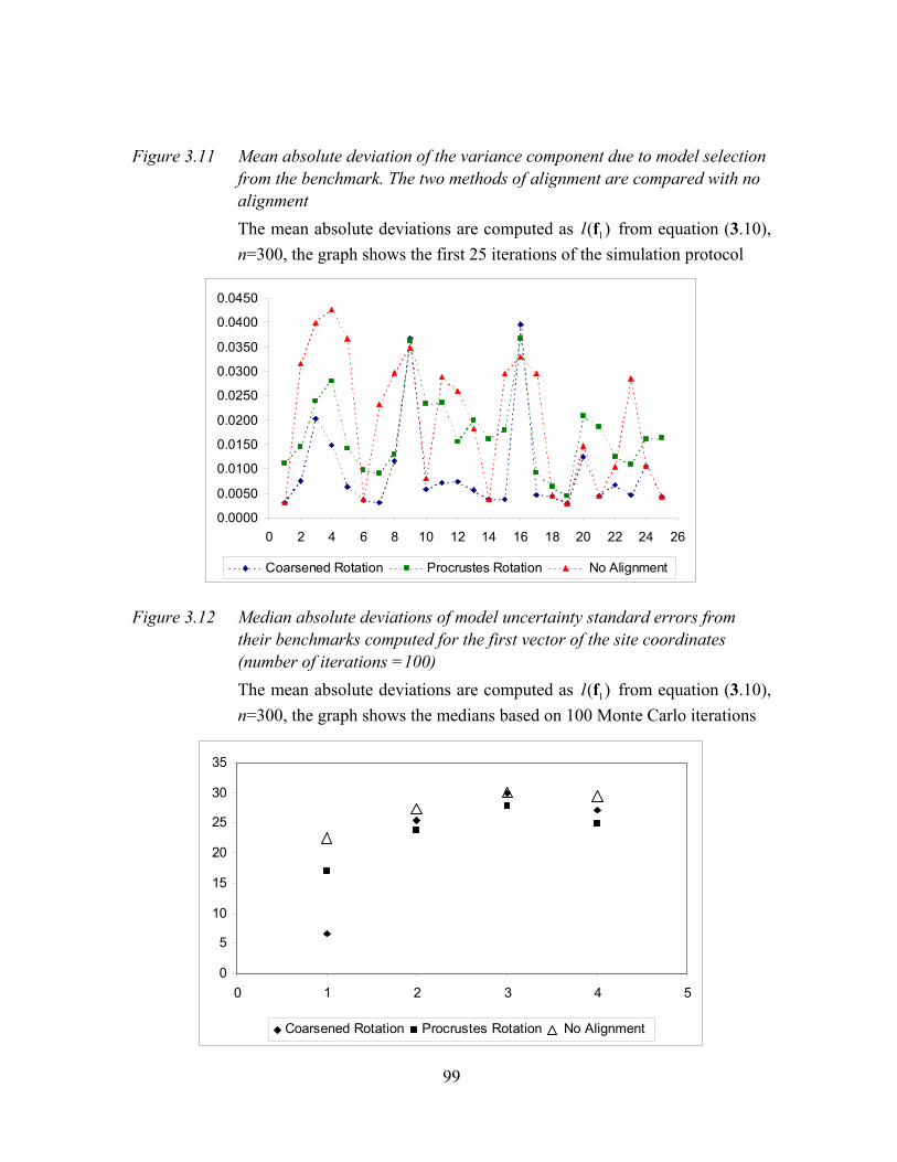
99

Figure 3.11 Mean absolute deviation of the variance component due to model selection from the benchmark. The two methods of alignment are compared with no alignment The mean absolute deviations are computed as 1( )l f from equation (3.10), n=300, the graph shows the first 25 iterations of the simulation protocol

0.0000

0.0050

0.0100

0.0150

0.0200

0.0250

0.0300

0.0350

0.0400

0.0450

0 2 4 6 8 10 12 14 16 18 20 22 24 26

Coarsened Rotation Procrustes Rotation No Alignment

Figure 3.12 Median absolute deviations of model uncertainty standard errors from their benchmarks computed for the first vector of the site coordinates (number of iterations =100) The mean absolute deviations are computed as 1( )l f from equation (3.10), n=300, the graph shows the medians based on 100 Monte Carlo iterations

0

5

10

15

20

25

30

35

0 1 2 3 4 5

Coarsened Rotation Procrustes Rotation No Alignment

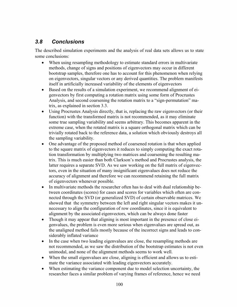
100

3.8 Conclusions The described simulation experiments and the analysis of real data sets allows us to state some conclusions:

• When using resampling methodology to estimate standard errors in multivariate methods, change of signs and positions of eigenvectors may occur in different bootstrap samples, therefore one has to account for this phenomenon when relying on eigenvectors, singular vectors or any derived quantities. The problem manifests itself in artificially increased variability of the elements of eigenvectors

• Based on the results of a simulation experiment, we recommend alignment of ei-genvectors by first computing a rotation matrix using some form of Procrustes Analysis, and second coarsening the rotation matrix to a “sign-permutation” ma-trix, as explained in section 3.3.

• Using Procrustes Analysis directly, that is, replacing the raw eigenvectors (or their function) with the transformed matrix is not recommended, as it may eliminate some true sampling variability and seems arbitrary. This becomes apparent in the extreme case, when the rotated matrix is a square orthogonal matrix which can be trivially rotated back to the reference data, a solution which obviously destroys all the sampling variability.

• One advantage of the proposed method of coarsened rotation is that when applied to the square matrix of eigenvectors it reduces to simply computing the exact rota-tion transformation by multiplying two matrices and coarsening the resulting ma-trix. This is much easier than both Clarkson’s method and Procrustes analysis, the latter requires a separate SVD. As we saw working on the full matrix of eigenvec-tors, even in the situation of many insignificant eigenvalues does not reduce the accuracy of alignment and therefore we can recommend retaining the full matrix of eigenvectors whenever possible.

• In multivariate methods the researcher often has to deal with dual relationship be-tween coordinates (scores) for cases and scores for variables which often are con-nected through the SVD (or generalized SVD) of certain observable matrices. We showed that the symmetry between the left and right singular vectors makes it un-necessary to align the configuration of row coordinates, since it is equivalent to alignment by the associated eigenvectors, which can be always done faster

• Though it may appear that aligning is most important in the presence of close ei-genvalues, the problem is even more serious when eigenvalues are spread out, as the unaligned method fails mostly because of the incorrect signs and leads to con-siderably inflated variance

• In the case when two leading eigenvalues are close, the resampling methods are not recommended, as we saw the distribution of the bootstrap estimates is not even unimodal, and none of the alignment methods seems to work well.

• When the small eigenvalues are close, aligning is efficient and allows us to esti-mate the variance associated with leading eigenvectors accurately.

• When estimating the variance component due to model selection uncertainty, the researcher faces a similar problem of varying frames of reference, hence we need

101

to align the eigenvectors to some fixed reference set. According to our limited simulation experience, described in section 7, (i) one does need to align the eigen-vectors when computing the component due to model selection uncertainty (ii) coarsened rotation again has its advantages over other methods of alignment

102

Chapter 4 Model Based Cluster and Outlier Analysis

4.1 Introduction This chapter is concerned with the implementation of cluster and outlier analyses via the MC3 approach that was used for variable selection in Chapter 2. The proposed approach is based on our understanding of the duality between selecting variables in statistical models and forming clusters or selecting observations in a multivariate data set. In our approach to cluster analysis, the model space is expanded to include all possible partitions of multi-variate observations. In outlier analysis, the model space is expanded to incorporate vari-ous subsets of observations. On the other hand, our method falls in the category of model-based cluster and outlier analysis, since each model is evaluated based on its likelihood. For cluster analysis we used penalized classification likelihood, and for outlier analysis we propose a new procedure that we call stochastic peeling, which is based on evaluating each subset of observations via some version of its penalized likelihood.

In cluster analysis, once we form the model space and the BIC criterion that allows us to compute the approximate Bayes Factor for any two models, we use the machinery of the MC3 method described in chapter 1 to navigate through the model space searching for data supported partitions of our data set. As always, the valuable output of the MC3 method is not only the solution (here, a set of clusters), but also a measure of uncertainty associated with each such partitioning. In particular, for each observation we can provide its activation probability in each of the given clusters. Each observation is allocated to a cluster with the highest posterior probability, max(pk), i=1..K (where K is the number of clusters). The uncertainty associated with class membership of any particular observation is formed simply as 1- max(pk).

Using penalized likelihood would allow us to potentially incorporate selection of variables simultaneously with forming clusters or outliers detection.

The chapter is organized as follows. First we provide a review of existing approaches in model based cluster analysis. In sections 4.2.2 through 4.2.5 we describe our basic algo-rithm for cluster analysis and show its strengths and weaknesses on some simulated ex-amples. A modified version of the algorithm is proposed in section 4.2.6 that incorporate the existing information about sub-clusters, which is used in formation of clusters. For example, the data may be collected in such a manner that there are groups of observations, perhaps associated with a river or river basin. The model space is formed in such a way that splitting sub-clusters is avoided. This method is applied to the analysis of a data set describing stressors/response relationship in one of the Ohio ecoregions. Finally, we de-

103

scribe a new method of outlier detection, which we call stochastic peeling and show its performance on several simulated and real-life examples (section 4.3).

4.2 Model Based Cluster Analysis via MC3

4.2.1 Existing approaches to Model Based Cluster Analysis Model based Cluster Analysis (MBCA) has recently attracted considerable attention. MBCA allows the researcher to divide a set of multivariate observations into clus-ters/classes so as to maximize the underlying likelihood function. The likelihood function measures how likely it is that the data, x, could have been generated from a particular classification structure. Two basic approaches exist to formulate the likelihood function: the classification likelihood method and the finite normal mixture approach. The former approach simply combines the likelihood (typically based on Gaussian distribution) func-tions from individual clusters to obtain an overall likelihood, given by expression (4.1)

1

( | , ) ( | , )i i

n

c ii

p f x ν νθ ν µ=

= Σ∏x (4.1)

where νi indicates the class membership for an observation (that is νi is an index of the class where the ith case belong).

In the mixture approach the likelihood is formed by mixing the observations across K clusters with mixing probabilities πk, associated with each cluster (see Banfield and Raftery, 1993; Bensmail et al., 1997; Fraley and Raftery, 1998). In the case of normal dis-tributions, the likelihood is given by:

11

( | ) ( | , )n K

m k i k kki

p f xπ µ==

= Σ∑∏x θ,π , (4.2)

where ,k kµ Σ are the mean and variance for the kth cluster. It was shown (Banfield and Raftery, 1993) that various heuristic methods of cluster analysis such as K-means and hi-erarchical methods naturally arise as special cases of maximizing these mixtures and clas-sification likelihoods under certain assumptions about the variance covariance matrices (Σk) of the associated clusters. Banfield and Raftery (1993) first suggest how the conven-tional heuristic approaches to cluster analysis can be generalized by considering various parsimonious parameterizations of the spectral decomposition of the variance covariance matrices. The main methods for the mixture likelihood are the EM algorithm and its sto-chastic version based on the Markov Chain Monte Carlo (Gibbs sampler). The MCMC approach allows the researcher to obtain the estimates of the uncertainties associated with the class membership of the observations that enhances the traditional analysis. The prob-lem of choosing the number of clusters and determining the most appropriate parameteri-

104

zation for the covariance matrices was considered in Fraley and Raftery (1998) and the solution was proposed via the Bayes Factors approach.

A natural extension of the likelihood mixture model is the model that allows the meas-urements for a response variable y to depend on a set of explanatory variables x via an ap-propriate likelihood function. The model based cluster analysis then is aimed at detecting clusters in such a way that the relationships between the response (y) and a set of predic-tors, x’s are explained well within each cluster. GLIMMIX (see Wedel and Kamakura, 1999) allows for a mixture of generalized linear models. This allows the user to employ cluster specific models for obtaining the predictions of the means of the explanatory vari-ables (see also McLachlan, & Peel, 2000).

In our work we propose another implementation of the model based cluster algorithm that also defines clusters in terms of the relationship between the set of y’s and the explanatory variables, x. We make use of the classification likelihood whose basic form is given by expression (4.1). Note that we can also write (4.1) via class membership variables, zik, where zik =1 when observation i belongs to a class j, and zik = 0 otherwise. For a normal regression model:

1 1

{ ( | , )} log{ ( | , )}K n

c ik i k kk i

log p z f x= =

= ∑∑x θ Z β Σ (4.3)

In our new method a proposed partitioning Zp is compared against any current partitioning Zc, using the difference of their classification BIC’s, as will be explained in the next sec-tion. Our approach can be easily extended to the situation with a multivariate response Y and it also lends itself to a general Reduced Rank Regression specification (see Van der Leeden, 1990).

4.2.2 The basic procedure In our study we propose the following procedure that is outlined below. This procedure falls in the general category of the Markov Chain Model Composition Monte Carlo (MC3) type. We define the states of our Markov Chain to be distinct partitions of n observations into k clusters (the number of clusters is a parameter that has to be known in advance). That is, a model (state) is described by a matrix with elements zik, where zik =1 when ob-servation i belongs to a class j, and zik = 0 otherwise. The neighborhood of each state, Z, is formed of all partitions (we use the terms “partition” and “model” interchangeably) such that any model in the neighborhood of Z can be obtained from Z by moving an ob-servation from a cluster k to a cluster k’, plus the partitioning of Z itself. The movements through the Markov chain are carried out as was explained in section 1.4.2 of Chapter 1.

First we generate an initial model (partition) by randomly allocating each observation to any of the available clusters, with the only restriction that the number of observations in each cluster must be not less than a pre-specified number (say κ where κ is a user-defined

105

constant). This way, any partition from a set of allowable partitions is equally likely. Therefore, at any stage of the process, a new proposed model is generated in the neighborhood of model, Z. The model is generated by randomly drawing an integer uni-formly distributed in the range from 1 to n. This is the index of the observation that has to be moved from its current cluster to another cluster (unless the number of observations in the cluster, nk, has reached its lower limit. If this is the case, we make another selection until we reach an observation that can be moved from its current cluster.). If there are only two clusters then the observation is moved to the other cluster; in case there are more than two clusters, the case is moved to a cluster that is randomly selected from the k-1 re-maining clusters.

The proposed model is evaluated based on the approximation to the Bayes Factor, ex-pressed via the associated BICs as shown below:

/

exp(0.5 )exp(0.5{ })

exp(0.5 )p

p c p cc

BICBF BIC BIC

BIC= = − (4.4)

where the BIC is expressed via the classification likelihood from the expression (4.1).

1 1

2 log{ ( | , )}

ˆ2 log ( | )

cK n

ik i kk i

BIC p penalty

z f x penalty= =

= −

= −∑∑

x θ Z

θ (4.5)

A proposed model, Z, is rejected or accepted if the ratio of the posterior probabilities (ap-proximated via (4.4)) is larger than 1. If the ratio is smaller than 1, it is compared with a realization of a uniform(0,1) random variable and the proposed model is accepted if the ratio is larger than the random number. Therefore, the proposed model is accepted with probability α.

{ }cpBF /,1min=α (4.6)

Now, we have to specify the penalty term in (4.5). We propose to form the penalty as an additive function of cluster-specific penalties, in this way we would be able to penalize each cluster separately for the number of variables in the associated model. This feature would allow for simultaneously partitioning of observations and selecting the relevant variables. A natural form of a penalty can be defined as follows:

1log( )

K

k kk

penalty n p=

= ∑

Assuming that clusters are formed with observations, k k k k= +y X β ε , where ~ (0, )k kN σε I , where Xk and yk are the subsets of the data that corresponds to a cluster k,

we can express (4.5) as follows.

106

'

1

2 { ( | )}ˆ ˆ( ) ( ){ log log( )}

c

Kk k k k k

k k kk k

BIC log p penalty

n p nn=

= −

− −= −∑

x θ

y X β y X β (4.7)

Notice that this algorithm requires the number of clusters to be specified in advance. Also it is important that the number of observations for each cluster is above a certain lower limit, as was already explained. The implementation of the algorithm is rather cumber-some and requires simultaneously maintaining several matrices of sums of squares and produces (SSCP) so as to be able to sweep the observations represented as dummy vari-ables in and out of clusters. Alternatively one can use the Sherman-Morrison-Woodbury formula to update the elements of the SSCP matrix, as explained in section 4.2.4. The out-put of the described procedure contains a set of models (partitions) which are filtered by the Occam’s window. The models that fall within Occam’s window are those whose ex-ponent of half difference with the BIC for the top model,

)})max({5.0exp( ii BICBIC −

exceed a certain lower limit. Each of the models is assigned a posterior probability by re-normalizing its respective BIC as follows:

∑=

=L

iiii BICBICDMp

1)5.0exp(/)5.0exp()|(ˆ ,

where L is the number of models in the output, Mi denotes a particular partitioning.

Choosing a single “best model” is accomplished via computing the estimates of posterior class membership probabilities for each observation, πik , i=1,..,n; k=1,..K.

{ : }

ˆ ˆ ( | )k

j M j

ik jM i

p M Dδ

π∈

= ∑ (4.8)

In words, we just add the estimated posterior probabilities for those partitions where a given observation is active in the k-th cluster. Once the class membership probabilities have been obtained, an observation is allocated to a cluster where it has the highest poste-rior probability. It is important to understand that allocating an observation to a cluster brings about uncertainty that has to be accounted for. A natural estimate of the class membership uncertainty is

1...ˆ1 max( )ik

k Kπ

=− .

4.2.3 Extensions for CCA and RDA The described clustering algorithm can be naturally extended to the case of RDA and CCA, described in 2.2. For this case, the BIC approximations derived in section 2.3.1 of Chapter 2 for different specifications of the variance-covariance matrix of model 2.14 that

107

can be applied to any given cluster should be replaced with its modification for the cluster algorithm from expression (4.5).

2

1 1

logK r

ik k kk i

BIC p nλ= =

= −

∑ ∑ (4.9)

where λk’s are the singular values of the matrix of fitted values for the kth cluster, kY .

4.2.4 Details on the Implementation The described algorithm incorporates both cases of univariate, multivariate, and reduced rank regressions. The algorithm employs the fact that deleting an observation from a model is computationally equivalent to adding a dummy variable whose value for the de-leted observation is set to 1 and for all other observations is set to 0, thus bearing a rela-tionship to outlier detection models. Therefore we can organize computations by provid-ing a dummy variable for each observation in a cluster and sweeping an observation in and out the augmented residual matrix of corrected sums of squares and cross products, CSSCP (after sweeping out the predictor variables). More specifically, the implementation of algorithm is as follows:

Step 1 (Initialization). Compute the matrix of corrected sums of squares and cross prod-ucts CSSCP on the augmented combined data, [ : : : ]n n1 X Y I (1n is the column of ones, and I is an n by n identity matrix). Sweep the CSSCP matrix on all p predic-tors included in the analysis, so as to compute the updated matrix, whose upper left corner will contain the following useful quantities:

−−

=−−

−−

Y)X)XX(X(IYYX)XX(YX)XX()XX(111

11

~~~~~~~~~~~~~~~~

]['''''

'''

pkCSSCP

based on the full set of observations, and YX ~,~ are centered versions of X and Y, and 1p is a vector of ones, of length p.

Fix the number of clusters, K and store K copies of CSSP. Randomly generate the model as a set of K vectors of indicators (one for each cluster),

1 2( , ,..., )k k k kM nδ δ δ=δ , k=1…K, where components {1/ 0}k

iδ = indicate whether the ith observation is included or excluded from the cluster k. Obviously, an observa-tion can be included in only one cluster, which means that its 1k

iδ = for some k,

then 0,li l kδ = ≠ .

Update each of the K copies of the CSSCPk [1p] matrices into CSSCPk[1p ,δM] by using the SWEEP operator on the subset k

Mδ (see Thisted, 1988). The upper left parts of these matrices will contain the following quantities.

108

−−

= −−

−−

δδδδδδδδδ

δδδδδδ

δY)X)XX(X(IYYX)XX(

YX)XX()XX(δ1 11

11

~~~~~~~~~~~~~~~~

],[ '''''

'''

MpkCSSCP

where δX~ and δY are the subset of rows of X and Y, respectively, corresponding

to the choice of observations in kMδ and now centered around the means of these

subsets, accordingly.

Compute the BIC approximation using one of its forms defined in previous sec-tions of the present chapter, for example, it can be as given by (4.9). Once BIC is computed for a certain model, (set of k

Mδ , k=1..K), its value, along with the BICk for individual clusters, is stored in a binary tree, so that next time when this model is encountered in the stochastic search procedure, the value of BIC could be quickly retrieved from the storage rather than recomputed from scratch.

Step i. Generate the proposed model ( kPMδ , k=1..K) from the neighborhood of the current

model ( kCMδ , k=1..K) from step (i-1), by randomly selecting an index j from the

set :{1,..,n} with probability 1/n. Find the kCMδ whose element 1k

jδ = and move the observation to another cluster by choosing one of the remaining K-1 clusters at random, say cluster l. Since ModelPM differs from ModelCM only by one observa-tion j , that has been exchanged between classes k and l, we compute ( k

PMδ , k=1..K) by performing a single sweep SWEEP[p+q+j] operator at the position p+q+j of CSSCPk [] (deleting an observation is like adding a variable!) and simi-larly we have to perform the reverse sweep if a variable is added, RSWEEP[p+q+j], for the CSSCPl [] matrix, since the observation is moved there. Check if the model is stored in the model tree and retrieve its BICPM from there. If the model has been encountered for the first time, compute BICPM. Compare BICPM to BICCM, if the ratio exp(0.5BICPM )/ exp(0.5BICCM) > 1, accept the pro-posed model, otherwise we accept the proposed model with acceptance probability

Pa =exp(0.5BICPM)/exp(0.5BICCM)

If the proposed model is accepted and it has not been visited yet, the associated BIC is stored in the tree structure; if the model has been already encountered in previous iterations, we increment the associated counter (number of times a given model has been visited) by one. If the proposed model is rejected we return to the current model ( k

CMδ , k=1..K) by performing a pair of SWEEP operators on CSSCPl [] and CSSCPk [], in the direction opposite to that used to update those matrices for the proposed model.

Comment A: To ensure appropriate mixing, we may want to perform random jumps in the model space, however one has to be cautious about matching the class labels. Obviously,

109

after we randomly generate another initial partitioning, it has to be aligned with respect to the partitions obtained in the previous chain. One way to do it is to evaluate the K! permu-tations of class labels in the initiated membership matrix Z and choose the one that maxi-mizes the (matrix) correlation between Z and the one corresponding to the highest BIC obtained in the previous chain of the algorithm.

Comment B: The described algorithm based on the augmented CSSCP matrix is accurate but requires substantial amounts of memory and time when sweeping across its p+q+n elements. A much faster but less accurate algorithm is based on updating the elements of the CSSCPk [1p] by using the fast updating formulas, as shown below. First the inverse of the δδ XX ~~ ' matrix after the ith case is deleted/added can be readily obtained by using the well known Sherman-Morrison-Woodbury formula:

ii

iii n x)XX(x

)XX(xx)XX()XX()XX( ~~~~/11

~~~~~~~~~~

1''

1''1'1'1'

−

−−−−

− −−+=

δδδ

δδδδδδδδ

ii

iii n x)XX(x

)XX(xx)XX()XX()XX( ~~~~/11

~~~~~~~~~~

1''

1''1'1'1'

−

−−−−

+ ++−=

δδδ

δδδδδδδδ ,

where, as before, subscript δ indicates a particular subset of observations that are present in the current cluster, nδ is the size of this set, and δxxx −= ii

~ is the vector of deviations from the cluster mean for the ith observation. Updating the current matrix of regression coefficients in the upper right corner of CSSCPk [1p] can be accomplished as follows. De-note δδδδδ YX)XX(Β 1 ~~~~ˆ '' −= , a p by q matrix of regression coefficient estimates for a clus-ter indexed by δ. Then deleting the ith case would result in,

ii

iiii n x)XX(x

xΒyx)XX(ΒΒ

1

1

~~~~/11)~ˆ~(~~~

ˆ,ˆ''

'''

−

− −=

δδδ

δδδδδ

mmmm

Finally the matrix of error sums of squares can be updated as follows. Let

δδδδδδ δY)X)XX(X(IYRSS 1 ~~~~~~ ''' −−= . Then it can be easily shown that after deleting ith

case:

ii

iiiii n x)XX(x

xΒyxΒyRSSRSS

1 ~~~~/11)~ˆ~)(~ˆ~(

,''

'''

−

−−=

δδδ

δδδδ

mmmm

Note, however that some of the numerical accuracy would be lost by using the updating formulas, since they involve explicit multiplications by the inverse of δδ XX ~~ ' .

Comment C: The described algorithm assumes that the same set of variables is used for each cluster, however an obvious modification would allow for simultaneous variable se-

110

lection within each cluster. The movements occur through the expanded model space de-fined as a combination of vectors, ( | )k k k

M p n p−=δ δ δ , whose first p components contain the indicators for variables selected for the kth cluster, and the remaining n-p components con-tain, as before, the indicators for observations. The Markov Chain is induced by defining the neighborhood of k

Mδ as a set of models that includes kMδ itself and all other models

that can be obtained from kMδ by either exchanging an observation between two clusters

or adding/deleting a variable in one of the clusters. In this version of the procedure, sweeping variables-observations is done simultaneously with sweeping actual variables.

Comment D: When movements occur in the combined variable/observation space, as de-scribed in the Comment C, computing the updating formulas stated in Comment B is a bit complicated since from the computational standpoint, the sets of variables designated to be X’s or Y’s changes with each sweep operation. Once an explanatory variable is in-cluded in the model and is swept in, it becomes an X, however once it is swept out of the model it joins the Y’s. Therefore, an additional bookkeeping is required when using the fast updating formulas so as to keep track of the designation of the X and Y sets.

4.2.5 Examples with simulated data To evaluate the performance and scope of usability of the developed procedure, several types of data exhibiting a cluster structure were simulated and the described procedure was applied. Consider a simple example (shown in Figure 4.1) of data with only one pre-dictor and two clusters (each cluster size is 100) that give rise to two types of regression lines. Our procedure had correctly allocated almost all but a few the observations. The un-certainty bars are based on the probabilities,

1...ˆ1 max( )ik

k Kπ

=− (the probability values were

multiplied by 20) and we show the observations that contain most uncertainty. The points with the greatest uncertainty lie at the intersection of the lines. This is as to be expected since these are the observations that can be fitted by either regression lines equally well.

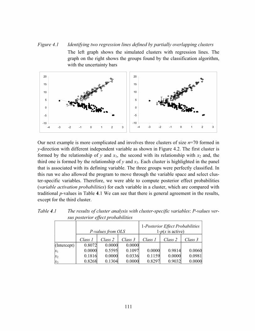
111

Figure 4.1 Identifying two regression lines defined by partially overlapping clusters The left graph shows the simulated clusters with regression lines. The graph on the right shows the groups found by the classification algorithm, with the uncertainty bars

-10

-5

0

5

10

15

20

-4 -3 -2 -1 0 1 2 3-10

-5

0

5

10

15

20

-4 -3 -2 -1 0 1 2 3

Our next example is more complicated and involves three clusters of size n=70 formed in y-direction with different independent variable as shown in Figure 4.2. The first cluster is formed by the relationship of y and x1, the second with its relationship with x2 and, the third one is formed by the relationship of y and x3. Each cluster is highlighted in the panel that is associated with its defining variable. The three groups were perfectly classified. In this run we also allowed the program to move through the variable space and select clus-ter-specific variables. Therefore, we were able to compute posterior effect probabilities (variable activation probabilities) for each variable in a cluster, which are compared with traditional p-values in Table 4.1 We can see that there is general agreement in the results, except for the third cluster.

Table 4.1 The results of cluster analysis with cluster-specific variables: P-values ver-sus posterior effect probabilities

P-values from OLS 1-Posterior Effect Probabilities

1-p(x is active)

Class 1 Class 2 Class 3 Class 1 Class 2 Class 3 (Intercept) 0.8072 0.0000 0.0000 x1 0.0000 0.5595 0.1097 0.0000 0.9814 0.0060x2 0.1816 0.0000 0.0336 0.1159 0.0000 0.0981x3 0.8268 0.1304 0.0000 0.8297 0.9032 0.0000

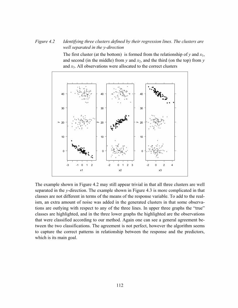
112

Figure 4.2 Identifying three clusters defined by their regression lines. The clusters are well separated in the y-direction The first cluster (at the bottom) is formed from the relationship of y and x1, and second (in the middle) from y and x2, and the third (on the top) from y and x3. All observations were allocated to the correct clusters

0

10

20

30

40

-3 -1 0 1 2

x1

y

0

10

20

30

40

-2 0 1 2 3

x2

y

0

10

20

30

40

-2 0 2 4

x3

y

The example shown in Figure 4.2 may still appear trivial in that all three clusters are well separated in the y-direction. The example shown in Figure 4.3 is more complicated in that classes are not different in terms of the means of the response variable. To add to the real-ism, an extra amount of noise was added in the generated clusters in that some observa-tions are outlying with respect to any of the three lines. In upper three graphs the “true” classes are highlighted, and in the three lower graphs the highlighted are the observations that were classified according to our method. Again one can see a general agreement be-tween the two classifications. The agreement is not perfect, however the algorithm seems to capture the correct patterns in relationship between the response and the predictors, which is its main goal.

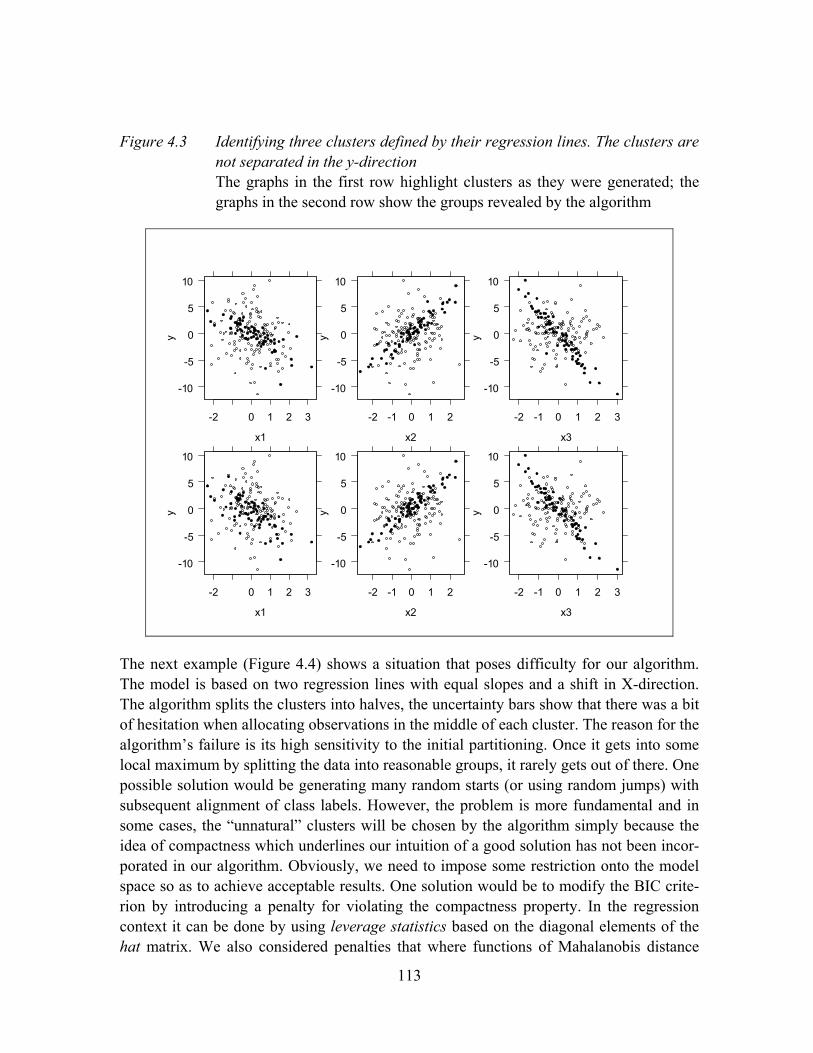
113

Figure 4.3 Identifying three clusters defined by their regression lines. The clusters are not separated in the y-direction The graphs in the first row highlight clusters as they were generated; the graphs in the second row show the groups revealed by the algorithm

-10

-5

0

5

10

-2 0 1 2 3

x1

y

-10

-5

0

5

10

-2 -1 0 1 2

x2

y

-10

-5

0

5

10

-2 -1 0 1 2 3

x3

y

-10

-5

0

5

10

-2 0 1 2 3

x1

y

-10

-5

0

5

10

-2 -1 0 1 2

x2

y

-10

-5

0

5

10

-2 -1 0 1 2 3

x3

y

The next example (Figure 4.4) shows a situation that poses difficulty for our algorithm. The model is based on two regression lines with equal slopes and a shift in X-direction. The algorithm splits the clusters into halves, the uncertainty bars show that there was a bit of hesitation when allocating observations in the middle of each cluster. The reason for the algorithm’s failure is its high sensitivity to the initial partitioning. Once it gets into some local maximum by splitting the data into reasonable groups, it rarely gets out of there. One possible solution would be generating many random starts (or using random jumps) with subsequent alignment of class labels. However, the problem is more fundamental and in some cases, the “unnatural” clusters will be chosen by the algorithm simply because the idea of compactness which underlines our intuition of a good solution has not been incor-porated in our algorithm. Obviously, we need to impose some restriction onto the model space so as to achieve acceptable results. One solution would be to modify the BIC crite-rion by introducing a penalty for violating the compactness property. In the regression context it can be done by using leverage statistics based on the diagonal elements of the hat matrix. We also considered penalties that where functions of Mahalanobis distance

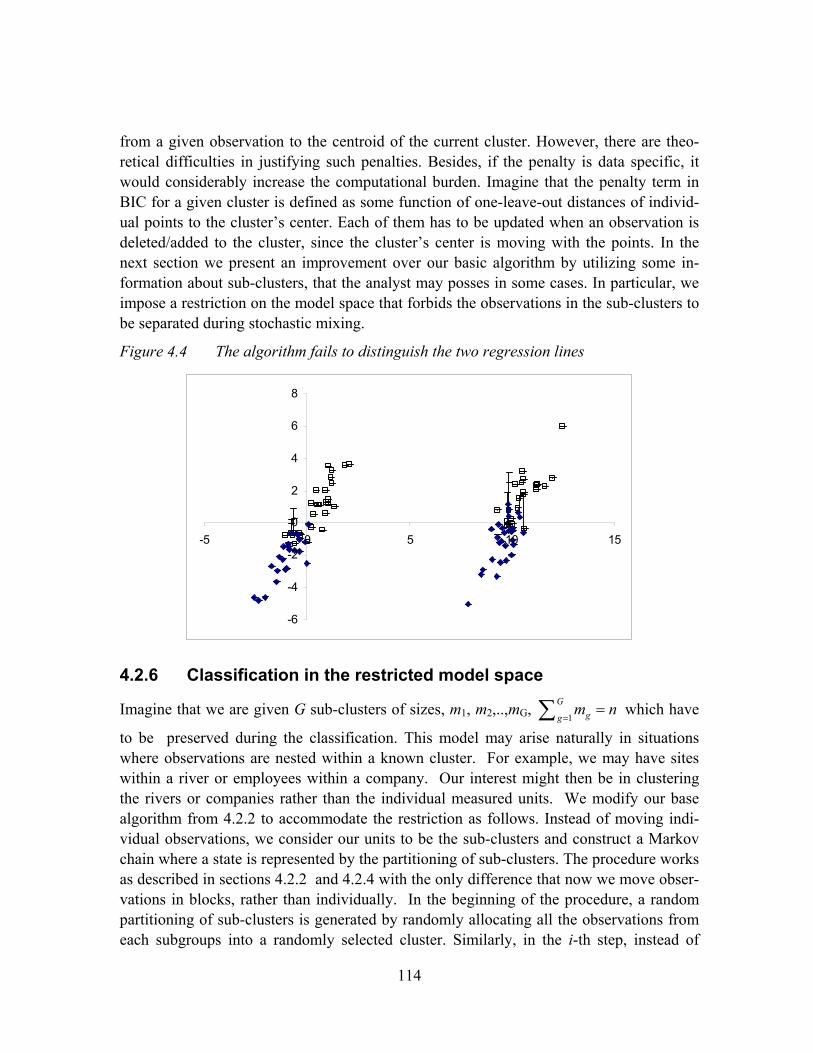
114

from a given observation to the centroid of the current cluster. However, there are theo-retical difficulties in justifying such penalties. Besides, if the penalty is data specific, it would considerably increase the computational burden. Imagine that the penalty term in BIC for a given cluster is defined as some function of one-leave-out distances of individ-ual points to the cluster’s center. Each of them has to be updated when an observation is deleted/added to the cluster, since the cluster’s center is moving with the points. In the next section we present an improvement over our basic algorithm by utilizing some in-formation about sub-clusters, that the analyst may posses in some cases. In particular, we impose a restriction on the model space that forbids the observations in the sub-clusters to be separated during stochastic mixing.

Figure 4.4 The algorithm fails to distinguish the two regression lines

-6

-4

-2

0

2

4

6

8

-5 0 5 10 15

4.2.6 Classification in the restricted model space

Imagine that we are given G sub-clusters of sizes, m1, m2,..,mG, 1

Ggg

m n=

=∑ which have

to be preserved during the classification. This model may arise naturally in situations where observations are nested within a known cluster. For example, we may have sites within a river or employees within a company. Our interest might then be in clustering the rivers or companies rather than the individual measured units. We modify our base algorithm from 4.2.2 to accommodate the restriction as follows. Instead of moving indi-vidual observations, we consider our units to be the sub-clusters and construct a Markov chain where a state is represented by the partitioning of sub-clusters. The procedure works as described in sections 4.2.2 and 4.2.4 with the only difference that now we move obser-vations in blocks, rather than individually. In the beginning of the procedure, a random partitioning of sub-clusters is generated by randomly allocating all the observations from each subgroups into a randomly selected cluster. Similarly, in the i-th step, instead of

115

choosing an individual observation, we choose a sub-cluster and reallocate all the observa-tions that fall within that group. Of course, computationally we are still dealing with col-umns of zeros and ones associated with individual cases, however this detail does not alter the desired features of Markov chain, which is defined now of the larger units. To ensure a better mixing, one may pick the sub-clusters with probabilities proportional to their sizes, rather than select them with probability 1/G. Notice that this modification will not require a change in the method for computing the acceptance ratio, α, in (4.6). Recall that the form of the rejection rule used in our MC3 procedure corresponds to that of the Metropolis algorithm, with the symmetric transition probability '( )q M M→ = '( )q M M→ . In our case, the transition probability is given by:

' 1( )1

gmq M M

n K→ =

−,

since we choose a sub-group with a probability proportional to its size and move it to a randomly selected cluster. However, we can go back to partitioning M with the same probability, ' 1( ) ( 1) /gq M M K m n−→ = − .

To see how the algorithm helps avoiding local minima, we tried the same example shown in Figure 4.4, now with 10 sub-clusters of size 5 located within each true cluster. The cor-rect model was found and the posterior probability of this model was visited in 95.5% of 3,000 iterations used in our MC3 procedure. Of course, this is an artificial example, where the sub-clusters are incorporated into the structure of true clusters. Our next example in section 4.9 is less obvious and the clusters are not so well defined.

4.2.7 An application: analysis of Ohio data The data are introduced in Norton (1999) and they contain variables that measure the bio-logical fish community along with possible chemical stressors and measures of the quality of habitat for one region in the state of Ohio (the eastern corn belt ecoregion). In this study we analyze the relationship between (i) the response given by the index of biological in-tegrity (IBI, an index computed as a weighted average of the originally transformed abun-dance of various fish species found on different sites), (ii) chemical stressors, such as the amount of DO (dissolved oxygen), Ph (phosphorus), and Zinc, (iii) the environmental fac-tors, measured by the qualitative habitat evaluation index, QHEI (it is a measure of habitat quality that combines scores for various factors related to stream gradient, in-stream cover score, siltation, etc). The data contain a large number of missing values and for the present analysis we selected a representative group of 330 cases with completed records. The data for the analysis were selected from various basins with the intention to cover most of the basins. Our goal is to divide the data into clusters based on the strength of the relationship between the IBI (the response) and the explanatory variables. This is different from the standard analysis in that the latter would classify the sites based on the within-cluster dis-

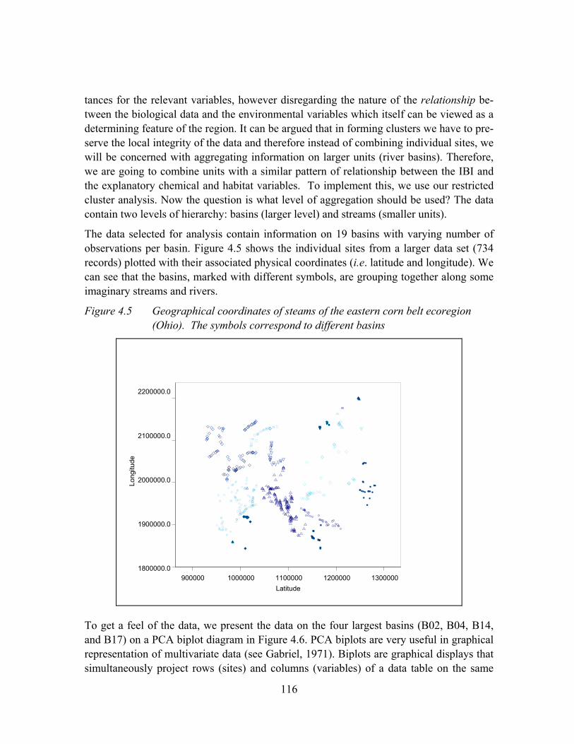
116

tances for the relevant variables, however disregarding the nature of the relationship be-tween the biological data and the environmental variables which itself can be viewed as a determining feature of the region. It can be argued that in forming clusters we have to pre-serve the local integrity of the data and therefore instead of combining individual sites, we will be concerned with aggregating information on larger units (river basins). Therefore, we are going to combine units with a similar pattern of relationship between the IBI and the explanatory chemical and habitat variables. To implement this, we use our restricted cluster analysis. Now the question is what level of aggregation should be used? The data contain two levels of hierarchy: basins (larger level) and streams (smaller units).

The data selected for analysis contain information on 19 basins with varying number of observations per basin. Figure 4.5 shows the individual sites from a larger data set (734 records) plotted with their associated physical coordinates (i.e. latitude and longitude). We can see that the basins, marked with different symbols, are grouping together along some imaginary streams and rivers.

Figure 4.5 Geographical coordinates of steams of the eastern corn belt ecoregion (Ohio). The symbols correspond to different basins

900000 1000000 1100000 1200000 1300000Latitude

1800000.0

1900000.0

2000000.0

2100000.0

2200000.0

Long

itude

To get a feel of the data, we present the data on the four largest basins (B02, B04, B14, and B17) on a PCA biplot diagram in Figure 4.6. PCA biplots are very useful in graphical representation of multivariate data (see Gabriel, 1971). Biplots are graphical displays that simultaneously project rows (sites) and columns (variables) of a data table on the same

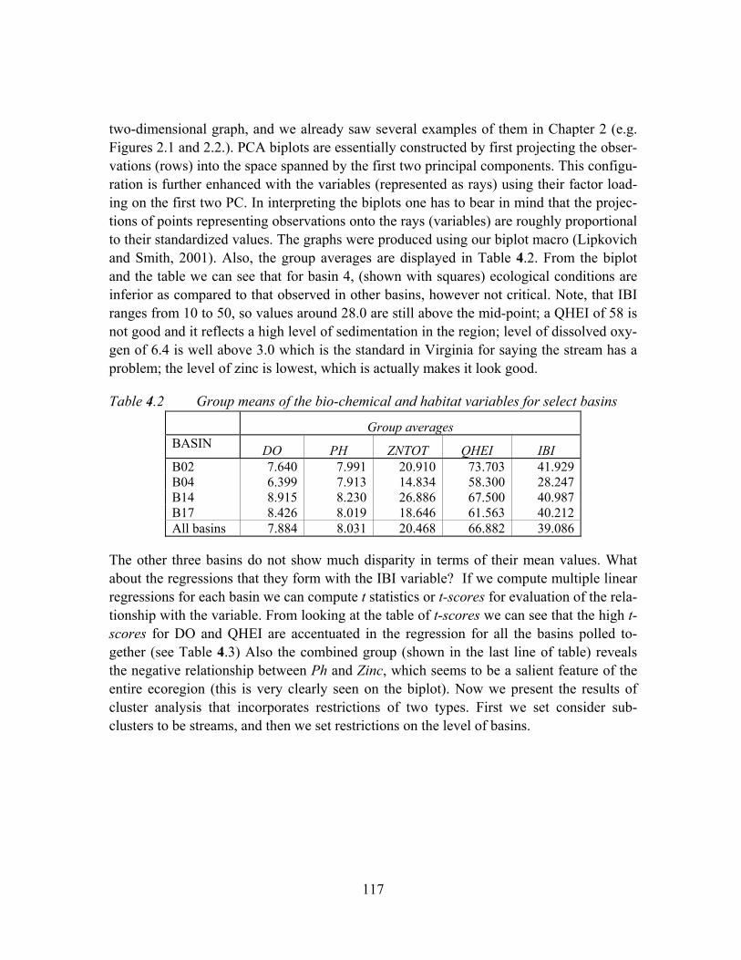
117

two-dimensional graph, and we already saw several examples of them in Chapter 2 (e.g. Figures 2.1 and 2.2.). PCA biplots are essentially constructed by first projecting the obser-vations (rows) into the space spanned by the first two principal components. This configu-ration is further enhanced with the variables (represented as rays) using their factor load-ing on the first two PC. In interpreting the biplots one has to bear in mind that the projec-tions of points representing observations onto the rays (variables) are roughly proportional to their standardized values. The graphs were produced using our biplot macro (Lipkovich and Smith, 2001). Also, the group averages are displayed in Table 4.2. From the biplot and the table we can see that for basin 4, (shown with squares) ecological conditions are inferior as compared to that observed in other basins, however not critical. Note, that IBI ranges from 10 to 50, so values around 28.0 are still above the mid-point; a QHEI of 58 is not good and it reflects a high level of sedimentation in the region; level of dissolved oxy-gen of 6.4 is well above 3.0 which is the standard in Virginia for saying the stream has a problem; the level of zinc is lowest, which is actually makes it look good.

Table 4.2 Group means of the bio-chemical and habitat variables for select basins Group averages BASIN DO PH ZNTOT QHEI IBI B02 7.640 7.991 20.910 73.703 41.929 B04 6.399 7.913 14.834 58.300 28.247 B14 8.915 8.230 26.886 67.500 40.987 B17 8.426 8.019 18.646 61.563 40.212 All basins 7.884 8.031 20.468 66.882 39.086

The other three basins do not show much disparity in terms of their mean values. What about the regressions that they form with the IBI variable? If we compute multiple linear regressions for each basin we can compute t statistics or t-scores for evaluation of the rela-tionship with the variable. From looking at the table of t-scores we can see that the high t-scores for DO and QHEI are accentuated in the regression for all the basins polled to-gether (see Table 4.3) Also the combined group (shown in the last line of table) reveals the negative relationship between Ph and Zinc, which seems to be a salient feature of the entire ecoregion (this is very clearly seen on the biplot). Now we present the results of cluster analysis that incorporates restrictions of two types. First we set consider sub-clusters to be streams, and then we set restrictions on the level of basins.

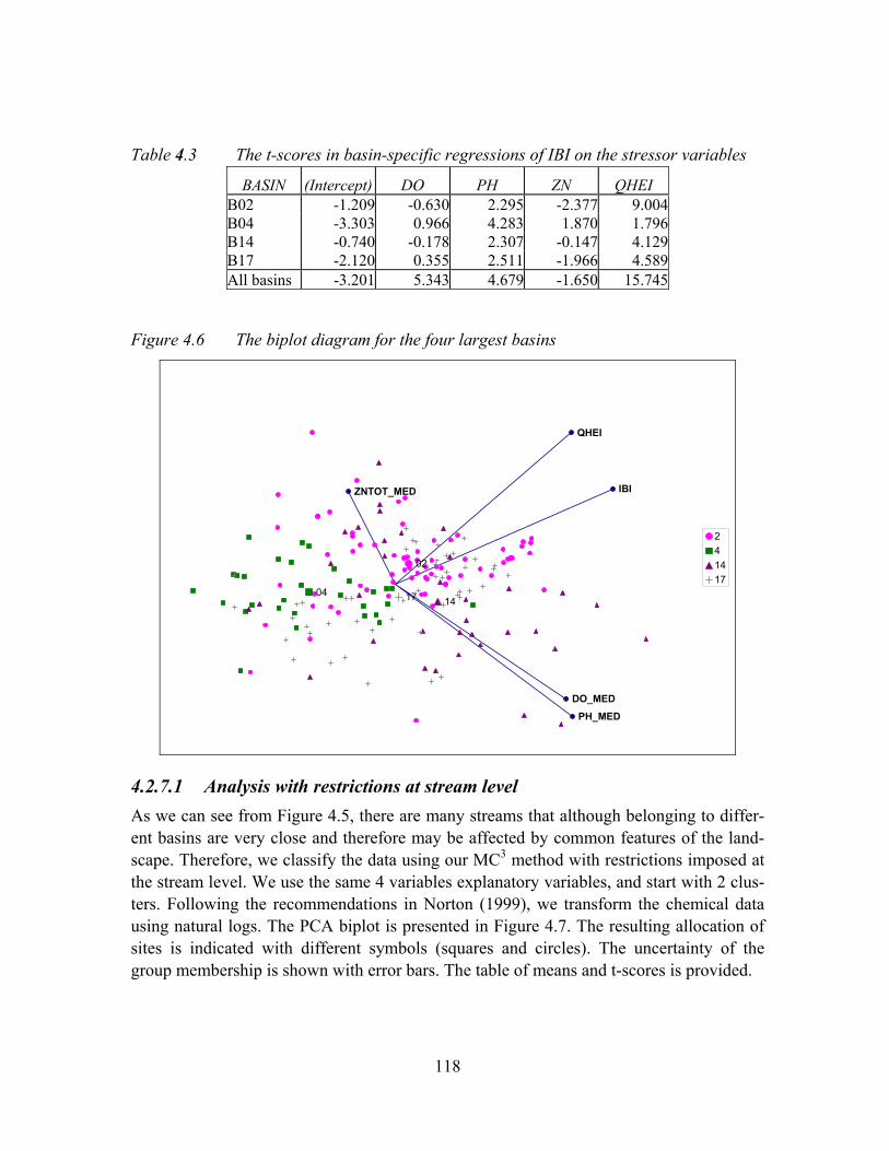
118

Table 4.3 The t-scores in basin-specific regressions of IBI on the stressor variables

BASIN (Intercept) DO PH ZN QHEI B02 -1.209 -0.630 2.295 -2.377 9.004B04 -3.303 0.966 4.283 1.870 1.796B14 -0.740 -0.178 2.307 -0.147 4.129B17 -2.120 0.355 2.511 -1.966 4.589All basins -3.201 5.343 4.679 -1.650 15.745

Figure 4.6 The biplot diagram for the four largest basins

QHEI

ZNTOT_MED

PH_MED

DO_MED

IBI

02

041417

241417

4.2.7.1 Analysis with restrictions at stream level As we can see from Figure 4.5, there are many streams that although belonging to differ-ent basins are very close and therefore may be affected by common features of the land-scape. Therefore, we classify the data using our MC3 method with restrictions imposed at the stream level. We use the same 4 variables explanatory variables, and start with 2 clus-ters. Following the recommendations in Norton (1999), we transform the chemical data using natural logs. The PCA biplot is presented in Figure 4.7. The resulting allocation of sites is indicated with different symbols (squares and circles). The uncertainty of the group membership is shown with error bars. The table of means and t-scores is provided.

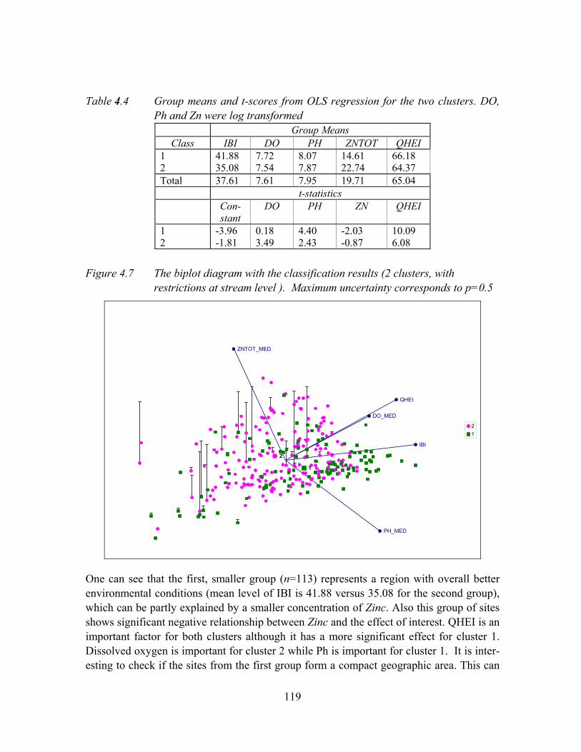
119

Table 4.4 Group means and t-scores from OLS regression for the two clusters. DO, Ph and Zn were log transformed

Group Means Class IBI DO PH ZNTOT QHEI

1 41.88 7.72 8.07 14.61 66.18 2 35.08 7.54 7.87 22.74 64.37 Total 37.61 7.61 7.95 19.71 65.04 t-statistics Con-

stant DO PH ZN QHEI

1 -3.96 0.18 4.40 -2.03 10.09 2 -1.81 3.49 2.43 -0.87 6.08

Figure 4.7 The biplot diagram with the classification results (2 clusters, with restrictions at stream level ). Maximum uncertainty corresponds to p=0.5

IBI

DO_MED

PH_MED

ZNTOT_MED

QHEI

2

1

21

One can see that the first, smaller group (n=113) represents a region with overall better environmental conditions (mean level of IBI is 41.88 versus 35.08 for the second group), which can be partly explained by a smaller concentration of Zinc. Also this group of sites shows significant negative relationship between Zinc and the effect of interest. QHEI is an important factor for both clusters although it has a more significant effect for cluster 1. Dissolved oxygen is important for cluster 2 while Ph is important for cluster 1. It is inter-esting to check if the sites from the first group form a compact geographic area. This can

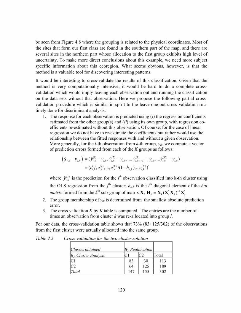
120

be seen from Figure 4.8 where the grouping is related to the physical coordinates. Most of the sites that form our first class are found in the southern part of the map, and there are several sites in the northern part whose allocation to the first group exhibits high level of uncertainty. To make more direct conclusions about this example, we need more subject specific information about this ecoregion. What seems obvious, however, is that the method is a valuable tool for discovering interesting patterns.

It would be interesting to cross-validate the results of this classification. Given that the method is very computationally intensive, it would be hard to do a complete cross-validation which would imply leaving each observation out and running the classification on the data sets without that observation. Here we propose the following partial cross-validation procedure which is similar in spirit to the leave-one-out cross validation rou-tinely done for discriminant analysis.

1. The response for each observation is predicted using (i) the regression coefficients estimated from the other group(s) and (ii) using its own group, with regression co-efficients re-estimated without this observation. Of course, for the case of linear regression we do not have to re-estimate the coefficients but rather would use the relationship between the fitted responses with and without a given observation. More generally, for the i-th observation from k-th group, yik we compute a vector of prediction errors formed from each of the K groups as follows:

( )' (1) (2) ( ) ( ) ', , , , , , , ,( ) , , ,

(1) (2) ( ) ( ) ', , , , ,

ˆ ˆ ˆ ˆ ˆ( , ,..., ,... )

( , ,..., /(1 ),... )

k Ki k i k i k i k i k i k i k i i k i k i k

k Ki k i k i k ii k i k

y y y y y y y y

e e e h e−− = − − − −

= −

y y

where ( ),ˆ j

i ky is the prediction for the ith observation classified into k-th cluster using the OLS regression from the jth cluster; hii,k is the ith diagonal element of the hat matrix formed from the kth sub-group of matrix X, ' 1 '( )k k k k k

−=H X X X X 2. The group membership of yik is determined from the smallest absolute prediction

error. 3. The cross validation K by K table is computed. The entries are the number of

times an observation from cluster k was re-allocated into group l.

For our data, the cross-validation table shows that 73% (83+125/302) of the observations from the first cluster were actually allocated into the same group.

Table 4.5 Cross-validation for the two cluster solution

Classes obtained By Reallocation By Cluster Analysis C1 C2 Total C1 83 30 113 C2 64 125 189 Total 147 155 302

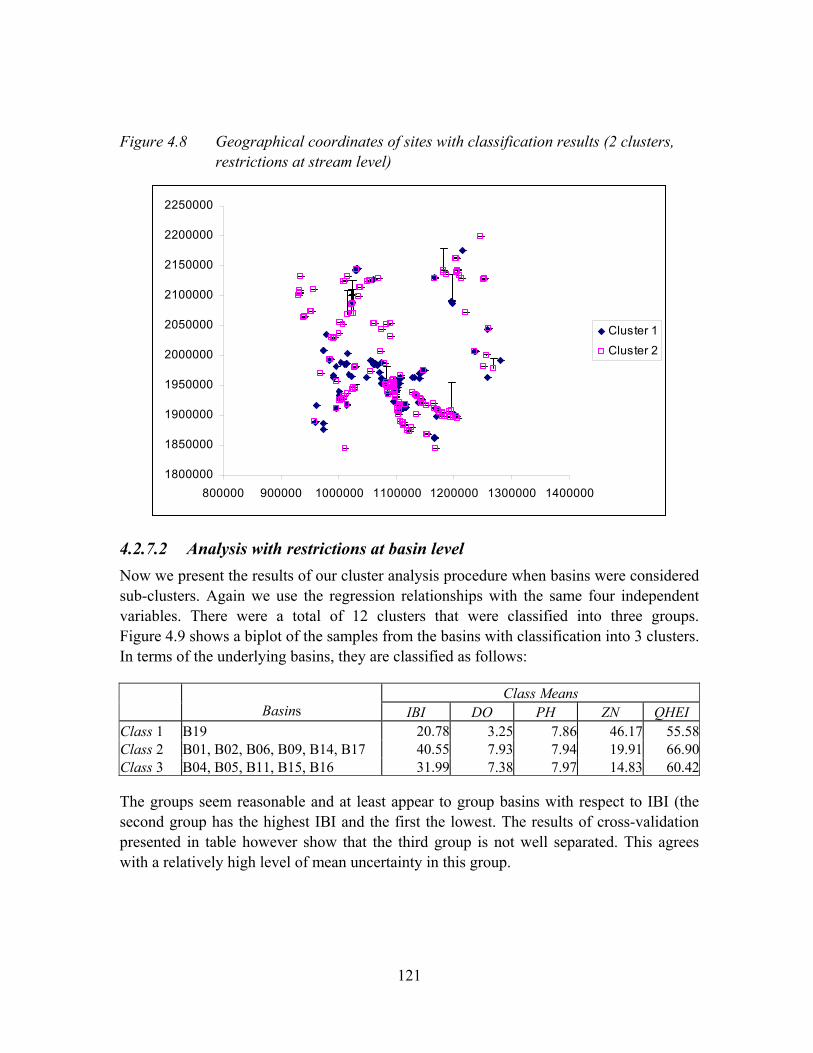
121

Figure 4.8 Geographical coordinates of sites with classification results (2 clusters, restrictions at stream level)

1800000

1850000

1900000

1950000

2000000

2050000

2100000

2150000

2200000

2250000

800000 900000 1000000 1100000 1200000 1300000 1400000

Cluster 1

Cluster 2

4.2.7.2 Analysis with restrictions at basin level Now we present the results of our cluster analysis procedure when basins were considered sub-clusters. Again we use the regression relationships with the same four independent variables. There were a total of 12 clusters that were classified into three groups. Figure 4.9 shows a biplot of the samples from the basins with classification into 3 clusters. In terms of the underlying basins, they are classified as follows:

Class Means Basins IBI DO PH ZN QHEI Class 1 B19 20.78 3.25 7.86 46.17 55.58Class 2 B01, B02, B06, B09, B14, B17 40.55 7.93 7.94 19.91 66.90Class 3 B04, B05, B11, B15, B16 31.99 7.38 7.97 14.83 60.42

The groups seem reasonable and at least appear to group basins with respect to IBI (the second group has the highest IBI and the first the lowest. The results of cross-validation presented in table however show that the third group is not well separated. This agrees with a relatively high level of mean uncertainty in this group.

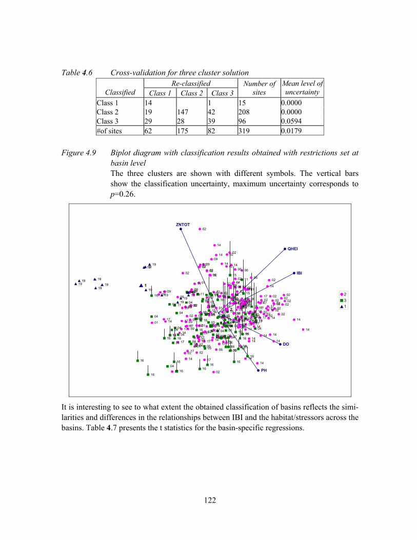
122

Table 4.6 Cross-validation for three cluster solution Re-classified

Classified Class 1 Class 2 Class 3 Number of

sites Mean level of uncertainty

Class 1 14 1 15 0.0000 Class 2 19 147 42 208 0.0000 Class 3 29 28 39 96 0.0594 #of sites 62 175 82 319 0.0179

Figure 4.9 Biplot diagram with classification results obtained with restrictions set at basin level The three clusters are shown with different symbols. The vertical bars show the classification uncertainty, maximum uncertainty corresponds to p=0.26.

QHEI

ZNTOT

PH

DO

IBI19

19

19

19

1919

191919

19

1919

19

1919

17

17

1717

1717

1717

17

17

17 17

17

17

1717

17

1717 17

17

17

17

17

1717

1717

17

17

17

17

17 17

17

17

1717

17

17171717

17

17

17

17

17

16

16

16

1616

16

16

16

16

16

16

16

16

16

16

16

16

16

1616

16

16

16

16

1615

15

1515

15

15

1515

15

15

151515 15

15

14

14

14

14

14

14

14

14

14

14

14

1414

1414

14

14

14

14

14

14

14

14

14

14

14

14

1414

14

1414

14

14

14

11

11

11

11

11

11

11

11 11

090909

09

0909

09

0909

09

09

09

09

09

0909

09

06 06

06

06

06

06

06

06

06

06

06

06

06

06

06

05

05 05

05

05

05

05

05

0505

05

0505

05

0505

05

04

04

04

04

0404 04

04

04

04

04

04

0404

04

04

04

04

04

04

04

04

04

04

04

04

04

04

0404

0202

02

02

02

02

02

02

02

02 02

02 02 02

020202

02

02

02

02

02

02

02

02

02

02

0202

02

02

02

02

02

0202

0202

02

02

02

02

02

020202

02

02

020202

02

0202

02

02

0202

02

02

02

02

02

02

02

02

0202

02

02

02

02 0101

0101

010101

01

01

01

0101

01

0101

01

01

0101

01

01

2

3

1

231

It is interesting to see to what extent the obtained classification of basins reflects the simi-larities and differences in the relationships between IBI and the habitat/stressors across the basins. Table 4.7 presents the t statistics for the basin-specific regressions.

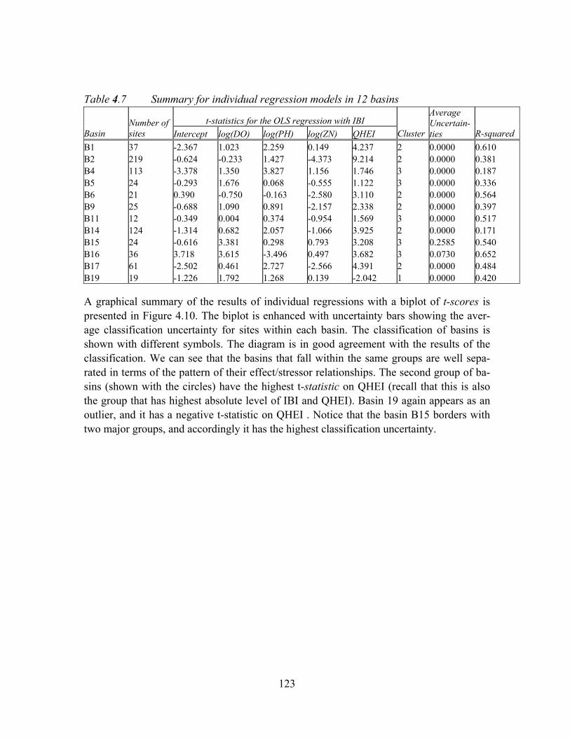
123

Table 4.7 Summary for individual regression models in 12 basins

t-statistics for the OLS regression with IBI Basin

Number of sites Intercept log(DO) log(PH) log(ZN) QHEI Cluster

Average Uncertain-ties R-squared

B1 37 -2.367 1.023 2.259 0.149 4.237 2 0.0000 0.610 B2 219 -0.624 -0.233 1.427 -4.373 9.214 2 0.0000 0.381 B4 113 -3.378 1.350 3.827 1.156 1.746 3 0.0000 0.187 B5 24 -0.293 1.676 0.068 -0.555 1.122 3 0.0000 0.336 B6 21 0.390 -0.750 -0.163 -2.580 3.110 2 0.0000 0.564 B9 25 -0.688 1.090 0.891 -2.157 2.338 2 0.0000 0.397 B11 12 -0.349 0.004 0.374 -0.954 1.569 3 0.0000 0.517 B14 124 -1.314 0.682 2.057 -1.066 3.925 2 0.0000 0.171 B15 24 -0.616 3.381 0.298 0.793 3.208 3 0.2585 0.540 B16 36 3.718 3.615 -3.496 0.497 3.682 3 0.0730 0.652 B17 61 -2.502 0.461 2.727 -2.566 4.391 2 0.0000 0.484 B19 19 -1.226 1.792 1.268 0.139 -2.042 1 0.0000 0.420

A graphical summary of the results of individual regressions with a biplot of t-scores is presented in Figure 4.10. The biplot is enhanced with uncertainty bars showing the aver-age classification uncertainty for sites within each basin. The classification of basins is shown with different symbols. The diagram is in good agreement with the results of the classification. We can see that the basins that fall within the same groups are well sepa-rated in terms of the pattern of their effect/stressor relationships. The second group of ba-sins (shown with the circles) have the highest t-statistic on QHEI (recall that this is also the group that has highest absolute level of IBI and QHEI). Basin 19 again appears as an outlier, and it has a negative t-statistic on QHEI . Notice that the basin B15 borders with two major groups, and accordingly it has the highest classification uncertainty.

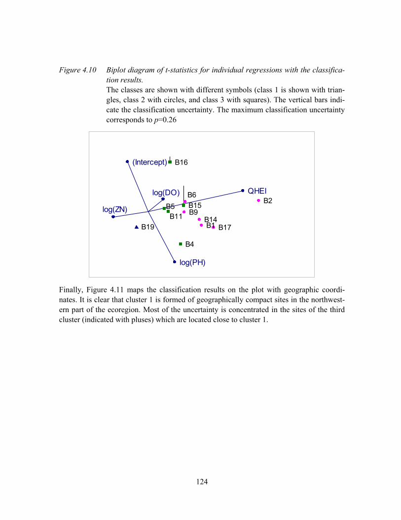
124

Figure 4.10 Biplot diagram of t-statistics for individual regressions with the classifica-tion results. The classes are shown with different symbols (class 1 is shown with trian-gles, class 2 with circles, and class 3 with squares). The vertical bars indi-cate the classification uncertainty. The maximum classification uncertainty corresponds to p=0.26

QHEI

log(ZN)

log(PH)

log(DO)

(Intercept)

B19 B17

B16

B15

B14B11 B9

B6B5

B4

B2

B1

Finally, Figure 4.11 maps the classification results on the plot with geographic coordi-nates. It is clear that cluster 1 is formed of geographically compact sites in the northwest-ern part of the ecoregion. Most of the uncertainty is concentrated in the sites of the third cluster (indicated with pluses) which are located close to cluster 1.

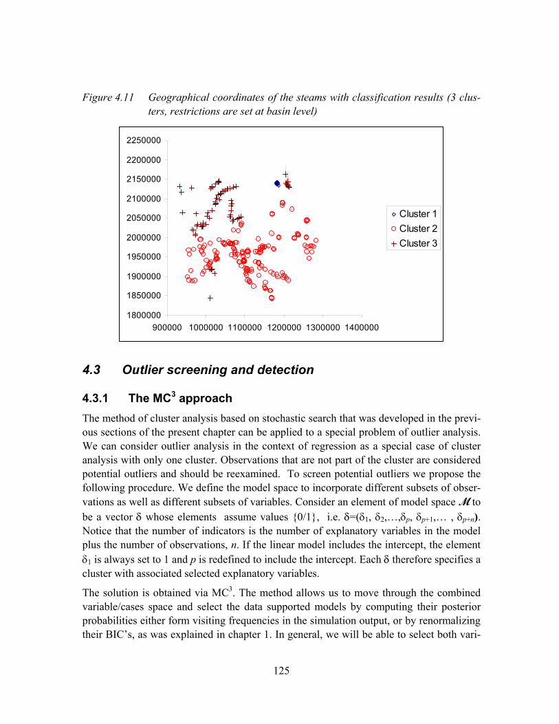
125

Figure 4.11 Geographical coordinates of the steams with classification results (3 clus-ters, restrictions are set at basin level)

1800000

1850000

1900000

1950000

2000000

2050000

2100000

2150000

2200000

2250000

900000 1000000 1100000 1200000 1300000 1400000

Cluster 1Cluster 2Cluster 3

4.3 Outlier screening and detection

4.3.1 The MC3 approach The method of cluster analysis based on stochastic search that was developed in the previ-ous sections of the present chapter can be applied to a special problem of outlier analysis. We can consider outlier analysis in the context of regression as a special case of cluster analysis with only one cluster. Observations that are not part of the cluster are considered potential outliers and should be reexamined. To screen potential outliers we propose the following procedure. We define the model space to incorporate different subsets of obser-vations as well as different subsets of variables. Consider an element of model space M to be a vector δ whose elements assume values {0/1}, i.e. δ=(δ1, δ2,…,δp, δp+1,… , δp+n). Notice that the number of indicators is the number of explanatory variables in the model plus the number of observations, n. If the linear model includes the intercept, the element δ1 is always set to 1 and p is redefined to include the intercept. Each δ therefore specifies a cluster with associated selected explanatory variables.

The solution is obtained via MC3. The method allows us to move through the combined variable/cases space and select the data supported models by computing their posterior probabilities either form visiting frequencies in the simulation output, or by renormalizing their BIC’s, as was explained in chapter 1. In general, we will be able to select both vari-

126

ables and observations simultaneously. A special case arises when we fix the variable composition and allow only the observations to move in and out of the model.

A Markov chain is induced by associating a combined subset of explanatory variables and cases, δi, with its neighborhood that includes δi along with any other model δ that differs from δi by one variable or one observation. A proposed model M is generated by selecting a random index i uniformly distributed from 1 to p+n. If this index falls within the range associated with the variables, (that is from 1 to p) a variable i is added to the model if it is missing in the current model, or it is dropped from the current model, if it is present. If the index falls within the range associated with the observations, that is from p+1 to n, the ob-servation with index i-p is added to the current model (cluster) if it is missing, or dropped from the current model if it is present in the model.

A similar approach was originally proposed in Hoeting et al. (1996) where a method of simultaneously selecting variables and multivariate outliers was implemented. Their ap-proach was based on computing and comparing posterior model probabilities for different models and it employed a closed form solution for the model posterior probabilities avail-able for the case of linear regression with normal errors (using the variance inflation out-lier model.) Also their analysis relied on a data prescreening procedure, namely they use least median of squares regression (LMS), which is a procedure with a high breakdown point (close to 0.5) due to Rousseeuw (1984) that allows a set of potential outliers to be detected before their proposed procedure can be applied. Our approach is more heuristic and in fact it can be considered a prescreening approach that would require a post-validation, as will be further explained. We use the BIC approximation to sort out models with high posterior probability, where models are the combinations of explanatory vari-ables and selected observations.

4.3.2 Development of BIC The form of the BIC criterion used for our outlier screening algorithm in the case of a uni-variate linear regression is as follows

*

0

ˆ( , ) /log logˆ( , ) /k k k

k kRSS n nBIC n p nRSS n nβ

= − −

β , (4.10)

where ˆ( , )k kRSS nβ is the residual sum of squares associated with the model δk (with nk

observations) and 0ˆ( , )RSS nβ is the residual sum of squares for the model with intercept

only based on the entire sample of n observations. This form is suggested by the argument similar to that used in constructing the adjusted R2 Here we are treating the deleted obser-vations as the extra variables added. The traditional BIC in the regression context (when the sample size is fixed) is

127

( )2

0

ˆ( )log log log 1 logˆ( )k

k k kRSSBIC n p n n R p nRSS β

= − − = − − −

β (4.11)

Of course, dividing by the RSS for the null model is irrelevant for computation of the Bayes Factor, since it will cancel out (and so will any constant added to BIC). However, this form of BIC is easy to interpret since it is directly related to such a traditional measure of model fit as the coefficient of determination. We need a similar criterion to evaluate how good our model is compared to the initial model with n observations. Now, when ob-servations are deleted from the model, it will be unfair to compare the residual sum of squares against the null sum of squares for the full sample, and it seems reasonable to di-vide each sum of squares by the appropriate sample size. This heuristic argument finds further support when we expand the expression (4.10) as follows:

( )* 2log 1 log logk k k k kk

nBIC n R p n nn

= − − − − (4.12)

Now we see that the adjustment for the sums of squares is equivalent to introducing a term that will penalize BIC for deleting observations. The penalty for deleting observations is similar to the penalty for including additional variables. This form of BIC can be used in our screening procedure. Note that the ratio of the minimum size of the cluster to the total sample size (nmin/n) should be bounded away from zero, otherwise we can always make the BIC infinitely large by reducing the number of observations to p, where p is the num-ber of explanatory variables. The residual sum of squares for the multiple regression of course can be made zero by choosing appropriately small subset of cases. Therefore the algorithm requires that the upper bound for the number of cases that can be deleted to be specified by the user. This tuning parameter controls the depth of screening and the proce-dure reminds one of peeling, since it tries to remove the upper depth% of the most outly-ing observations, hence we call it stochastic peeling

Another way to look at the expression (4.12) is by observing that its extra penalty term can be accommodated in the appropriate adjustment of the prior model probability, P(Mk) using the duality between the specification of penalties and model priors that was noted in Noble (2000). Indeed, if we look at the expression for the rejection constant, α in the ex-pression (1.11) of the base Metropolis algorithm that is used in our MC3 procedure, we can see that any additive term in BIC can be absorbed by the ratio of model priors.

1 1 1 1 1 1

0 0 0 0 0 0

( | ) ( ) exp(0.5 ) ( ) exp(0.5 2ln( ( )) ( | ) ( ) exp(0.5 ) ( ) exp(0.5 2ln( ( ))p D M p M BIC p M BIC cp Mp D M p M BIC p M BIC cp M

−≈ =

+

where c is an arbitrary constant. Apparently we can go the other way around and factor out an additive penalty from BIC* as an additional factor for the model priors. Assuming that initially our model priors p(M1) and p(M0) are equal, we can assign them non-trivial values so as to turn our BIC* into BIC from (4.11). Let M0 denote the full model, which in

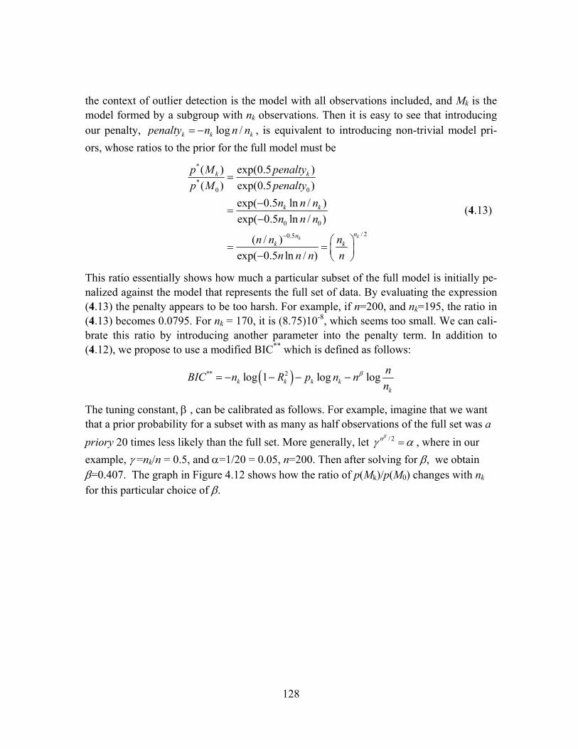
128

the context of outlier detection is the model with all observations included, and Mk is the model formed by a subgroup with nk observations. Then it is easy to see that introducing our penalty, log /k k kpenalty n n n= − , is equivalent to introducing non-trivial model pri-ors, whose ratios to the prior for the full model must be

*

*0 0

0 0/ 20.5

( ) exp(0.5 )( ) exp(0.5 )

exp( 0.5 ln / )exp( 0.5 ln / )

( / )exp( 0.5 ln / )

kk

k k

k k

nnk k

p M penaltyp M penalty

n n nn n n

n n nn n n n

−

=

−=

−

= = −

(4.13)

This ratio essentially shows how much a particular subset of the full model is initially pe-nalized against the model that represents the full set of data. By evaluating the expression (4.13) the penalty appears to be too harsh. For example, if n=200, and nk=195, the ratio in (4.13) becomes 0.0795. For nk = 170, it is (8.75)10-8, which seems too small. We can cali-brate this ratio by introducing another parameter into the penalty term. In addition to (4.12), we propose to use a modified BIC** which is defined as follows:

( )** 2log 1 log logk k k kk

nBIC n R p n nn

β= − − − −

The tuning constant, β , can be calibrated as follows. For example, imagine that we want that a prior probability for a subset with as many as half observations of the full set was a priory 20 times less likely than the full set. More generally, let / 2nβγ α= , where in our example, γ =nk/n = 0.5, and α=1/20 = 0.05, n=200. Then after solving for β, we obtain β=0.407. The graph in Figure 4.12 shows how the ratio of p(Mk)/p(M0) changes with nk for this particular choice of β.

129

Figure 4.12 Relationship between p(Mk)/p(M0) and the sample size, nk for β=0.407, n=200

0.000.100.200.300.400.500.600.700.800.901.00

0 50 100 150 200

4.3.3 Implementation Implementation of the algorithm is very similar to that for the cluster analysis method de-scribed in section 4.2.4. Computationally, the only difference is that now we have to deal with only one “cluster”, hence we have to maintain and update only one matrix of sums of squares and cross products. Like we did with K clusters, we augment the CSSCP matrix with an n by n identity matrix and sweep the observations represented as dummy variables in and out. Alternatively, the Sherman-Morrison-Woodbury formula can be used to update the elements of the CSSCP matrix as was explained in section 4.2.4.

The output of the described procedure contains a set of models (selected observations). Each model is assigned a posterior probability by renormalizing its respective BIC as fol-lows:

∑=

=L

iiii BICBICDMp

1)5.0exp(/)5.0exp()|(ˆ ,

where L is the number of models in the output, Mi denotes a particular partition.

As it was done with variables, for each observation their activation probability can be computed, by adding the estimated posterior probabilities for those subsets where a given observation is active.

ˆ ˆ( | ) ( | )Ml

li

p i D p M Dδ∈

= ∑ (4.14)

130

By subtracting this probability from 1.0, we obtain the probability that a given observation is an outlier. Displaying this probability on a scree plot facilitates detecting gross outliers. If the depth parameter is set too high, there is a danger that too many observations would be considered outliers. Therefore, we consider our screening procedure as only the first step in a more comprehensive treatment. The hope is that even if too many outliers would be “detected”, the remaining observations would reveal the true regression plane, which now can be used to iteratively reallocate deleted observations. This can be accomplished by comparing the distance from each removed point to the regression plane in the y direc-tion scaled by a robust estimate of standard deviation based on residuals from the OLS regression, with the percentile points of t-distribution. For the estimate of standard devia-

tion we can use a robust MAD estimate, 6745.0

|)(|ˆ iimad

ymedianymedian −=σ .

4.3.4 Examples with simulated data To evaluate the approach a simulation was used. In the simulation, we used a general variance-inflation and shift model of outliers. We simulated 200 observations as follows:

'i i iy δε= + ∆ +x β , εi~N(0,σ2), where:

0

1 0

1, , 1with p pwith p p

δδ

== = −

0

1 0

0, , 1with p pwith p p

=∆ = ∆ = −

Here, p is the probability of generating a potential outlier. Several simulated data sets were analyzed with our outlier detection algorithm and the results are presented in the nest two Figures. The first example uses δ1=7, p0=0.5, ∆1=0, with a single explanatory vari-able. Therefore, this is a variance inflation model with zero shift. We ran 3000 iterations of our outlier detection algorithm with the depth parameter set to 30 observations, which means that is in each model at least 170 observations have to be selected. Figure 4.13 shows the scatter plot of the data with error bars indicating the outlier probability,

ˆ1 ( | )p i D− , for each observation. We can see that most of the actual outliers were de-tected, as the associated probabilities are high.

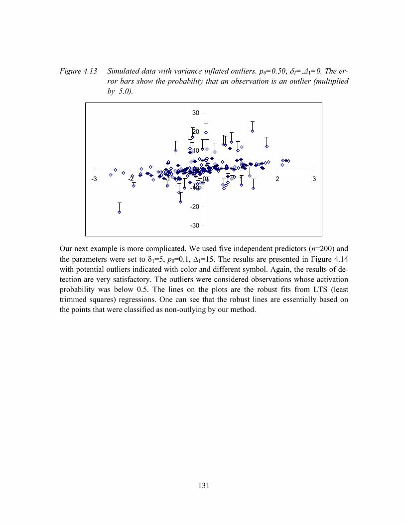
131

Figure 4.13 Simulated data with variance inflated outliers. p0=0.50, δ1=,∆1=0. The er-ror bars show the probability that an observation is an outlier (multiplied by 5.0).

-30

-20

-10

0

10

20

30

-3 -2 -1 0 1 2 3

Our next example is more complicated. We used five independent predictors (n=200) and the parameters were set to δ1=5, p0=0.1, ∆1=15. The results are presented in Figure 4.14 with potential outliers indicated with color and different symbol. Again, the results of de-tection are very satisfactory. The outliers were considered observations whose activation probability was below 0.5. The lines on the plots are the robust fits from LTS (least trimmed squares) regressions. One can see that the robust lines are essentially based on the points that were classified as non-outlying by our method.

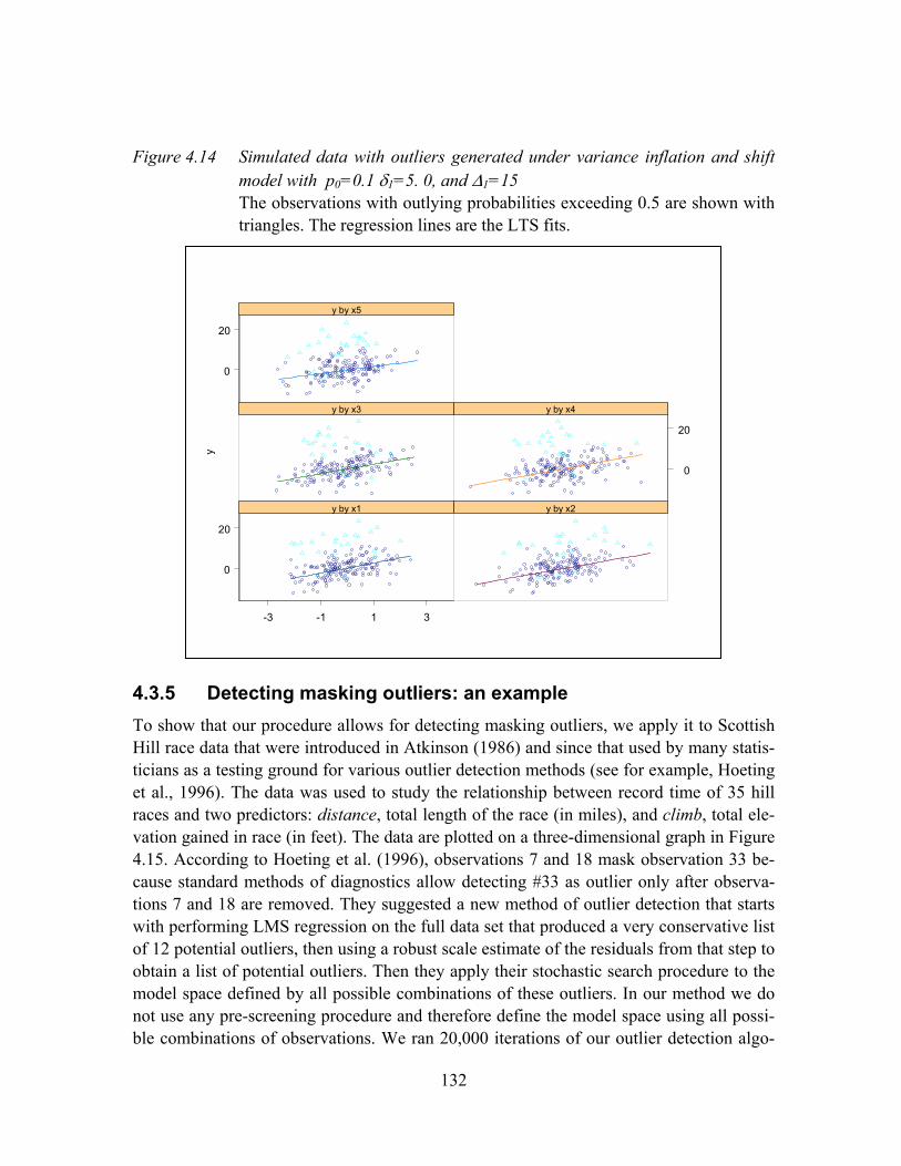
132

Figure 4.14 Simulated data with outliers generated under variance inflation and shift model with p0=0.1 δ1=5. 0, and ∆1=15 The observations with outlying probabilities exceeding 0.5 are shown with triangles. The regression lines are the LTS fits.

4.3.5 Detecting masking outliers: an example To show that our procedure allows for detecting masking outliers, we apply it to Scottish Hill race data that were introduced in Atkinson (1986) and since that used by many statis-ticians as a testing ground for various outlier detection methods (see for example, Hoeting et al., 1996). The data was used to study the relationship between record time of 35 hill races and two predictors: distance, total length of the race (in miles), and climb, total ele-vation gained in race (in feet). The data are plotted on a three-dimensional graph in Figure 4.15. According to Hoeting et al. (1996), observations 7 and 18 mask observation 33 be-cause standard methods of diagnostics allow detecting #33 as outlier only after observa-tions 7 and 18 are removed. They suggested a new method of outlier detection that starts with performing LMS regression on the full data set that produced a very conservative list of 12 potential outliers, then using a robust scale estimate of the residuals from that step to obtain a list of potential outliers. Then they apply their stochastic search procedure to the model space defined by all possible combinations of these outliers. In our method we do not use any pre-screening procedure and therefore define the model space using all possi-ble combinations of observations. We ran 20,000 iterations of our outlier detection algo-

-3 -1 1 3

0

20

0

20

0

20

y

y by x1 y by x2

y by x3 y by x4

y by x5

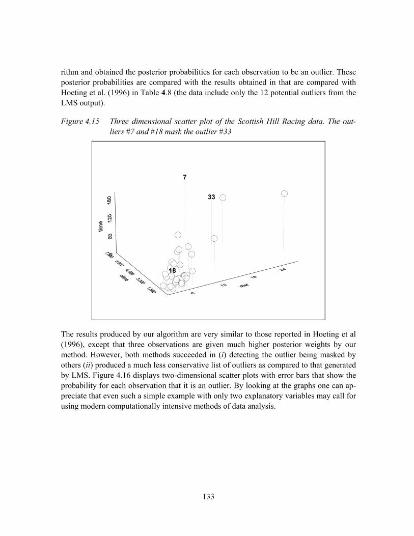
133

rithm and obtained the posterior probabilities for each observation to be an outlier. These posterior probabilities are compared with the results obtained in that are compared with Hoeting et al. (1996) in Table 4.8 (the data include only the 12 potential outliers from the LMS output).

Figure 4.15 Three dimensional scatter plot of the Scottish Hill Racing data. The out-liers #7 and #18 mask the outlier #33

7

18

33

The results produced by our algorithm are very similar to those reported in Hoeting et al (1996), except that three observations are given much higher posterior weights by our method. However, both methods succeeded in (i) detecting the outlier being masked by others (ii) produced a much less conservative list of outliers as compared to that generated by LMS. Figure 4.16 displays two-dimensional scatter plots with error bars that show the probability for each observation that it is an outlier. By looking at the graphs one can ap-preciate that even such a simple example with only two explanatory variables may call for using modern computationally intensive methods of data analysis.

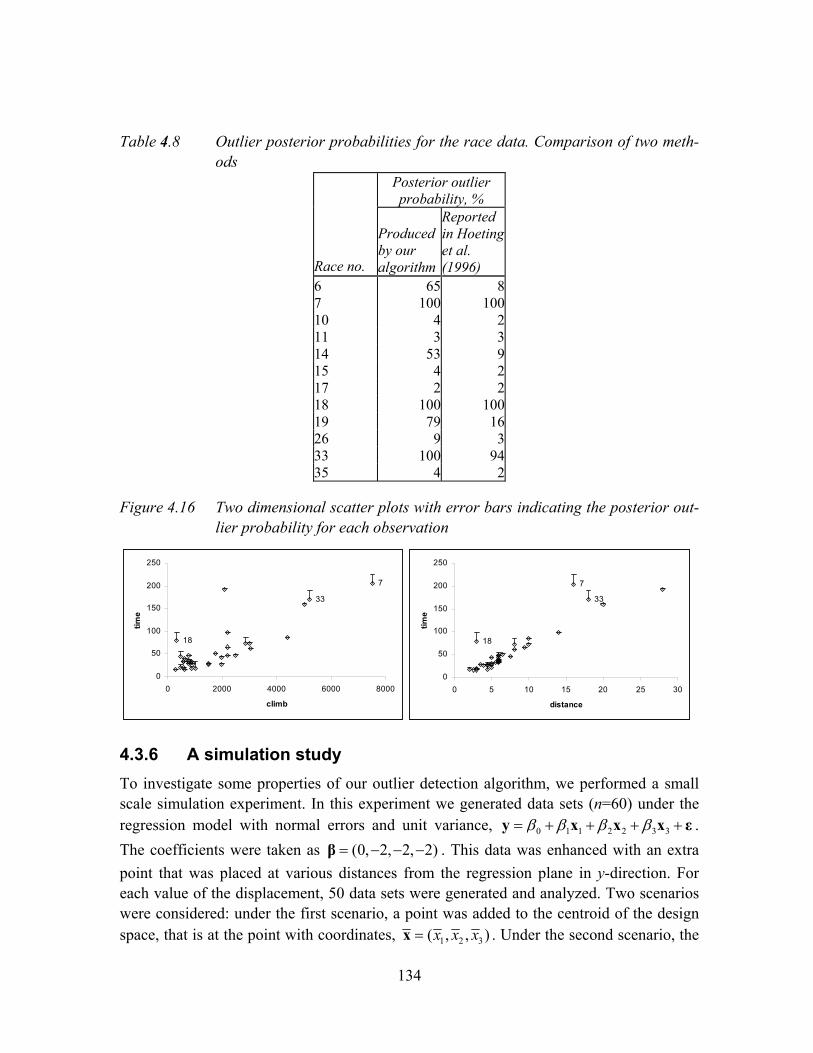
134

Table 4.8 Outlier posterior probabilities for the race data. Comparison of two meth-ods

Posterior outlier probability, %

Race no.

Produced by our algorithm

Reported in Hoeting et al. (1996)

6 65 87 100 10010 4 211 3 314 53 915 4 217 2 218 100 10019 79 1626 9 333 100 9435 4 2

Figure 4.16 Two dimensional scatter plots with error bars indicating the posterior out-lier probability for each observation

33

18

7

0

50

100

150

200

250

0 2000 4000 6000 8000

climb

time

33

18

7

0

50

100

150

200

250

0 5 10 15 20 25 30

distance

time

4.3.6 A simulation study To investigate some properties of our outlier detection algorithm, we performed a small scale simulation experiment. In this experiment we generated data sets (n=60) under the regression model with normal errors and unit variance, 0 1 1 2 2 3 3β β β β= + + + +y x x x ε . The coefficients were taken as (0, 2, 2, 2)= − − −β . This data was enhanced with an extra point that was placed at various distances from the regression plane in y-direction. For each value of the displacement, 50 data sets were generated and analyzed. Two scenarios were considered: under the first scenario, a point was added to the centroid of the design space, that is at the point with coordinates, 1 2 3( , , )x x x=x . Under the second scenario, the

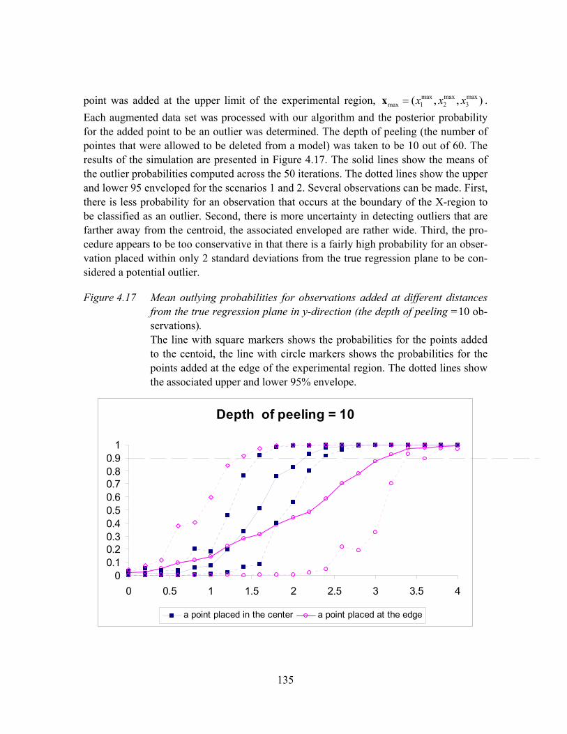
135

point was added at the upper limit of the experimental region, max max maxmax 1 2 3( , , )x x x=x .

Each augmented data set was processed with our algorithm and the posterior probability for the added point to be an outlier was determined. The depth of peeling (the number of pointes that were allowed to be deleted from a model) was taken to be 10 out of 60. The results of the simulation are presented in Figure 4.17. The solid lines show the means of the outlier probabilities computed across the 50 iterations. The dotted lines show the upper and lower 95 enveloped for the scenarios 1 and 2. Several observations can be made. First, there is less probability for an observation that occurs at the boundary of the X-region to be classified as an outlier. Second, there is more uncertainty in detecting outliers that are farther away from the centroid, the associated enveloped are rather wide. Third, the pro-cedure appears to be too conservative in that there is a fairly high probability for an obser-vation placed within only 2 standard deviations from the true regression plane to be con-sidered a potential outlier.

Figure 4.17 Mean outlying probabilities for observations added at different distances from the true regression plane in y-direction (the depth of peeling =10 ob-servations). The line with square markers shows the probabilities for the points added to the centoid, the line with circle markers shows the probabilities for the points added at the edge of the experimental region. The dotted lines show the associated upper and lower 95% envelope.

Depth of peeling = 10

00.10.20.30.40.50.60.70.80.9

1

0 0.5 1 1.5 2 2.5 3 3.5 4

a point placed in the center a point placed at the edge

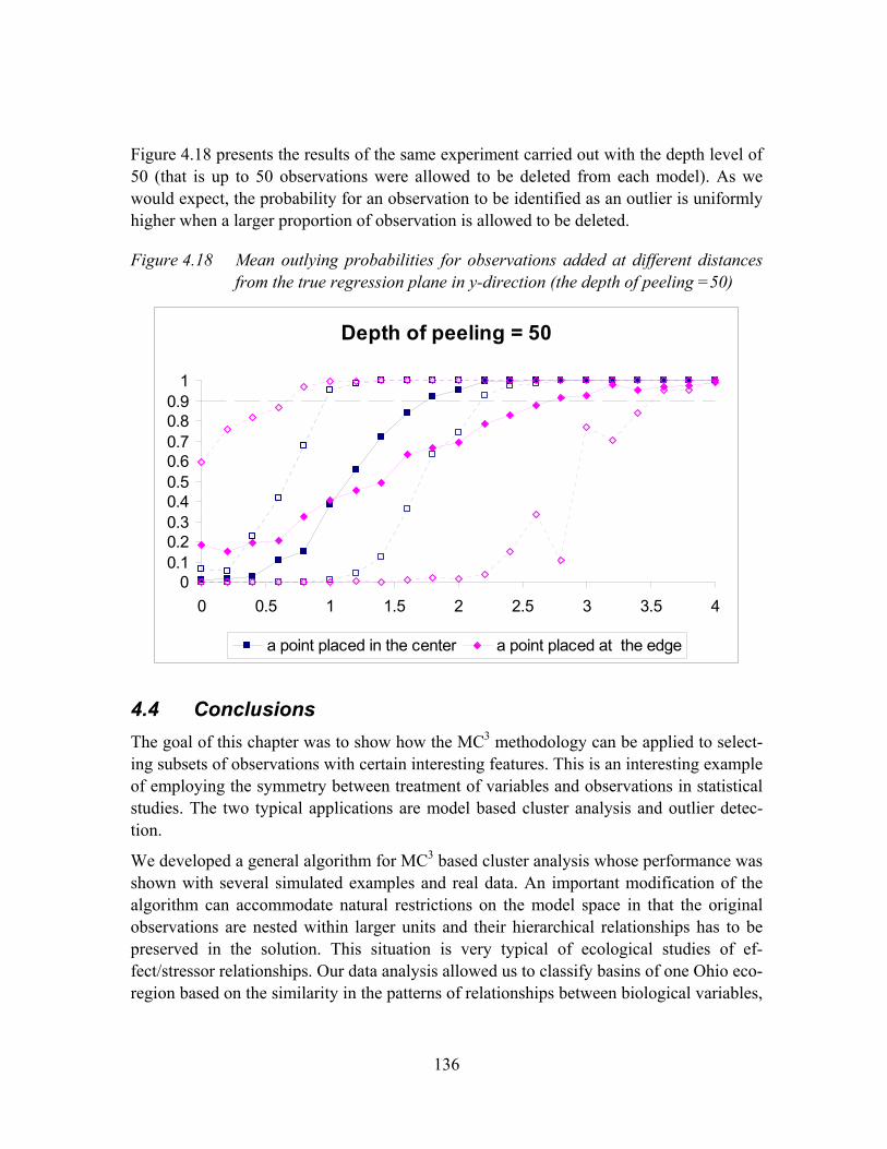
136

Figure 4.18 presents the results of the same experiment carried out with the depth level of 50 (that is up to 50 observations were allowed to be deleted from each model). As we would expect, the probability for an observation to be identified as an outlier is uniformly higher when a larger proportion of observation is allowed to be deleted.

Figure 4.18 Mean outlying probabilities for observations added at different distances from the true regression plane in y-direction (the depth of peeling =50)

Depth of peeling = 50

00.10.20.30.40.50.60.70.80.9

1

0 0.5 1 1.5 2 2.5 3 3.5 4

a point placed in the center a point placed at the edge

4.4 Conclusions The goal of this chapter was to show how the MC3 methodology can be applied to select-ing subsets of observations with certain interesting features. This is an interesting example of employing the symmetry between treatment of variables and observations in statistical studies. The two typical applications are model based cluster analysis and outlier detec-tion.

We developed a general algorithm for MC3 based cluster analysis whose performance was shown with several simulated examples and real data. An important modification of the algorithm can accommodate natural restrictions on the model space in that the original observations are nested within larger units and their hierarchical relationships has to be preserved in the solution. This situation is very typical of ecological studies of ef-fect/stressor relationships. Our data analysis allowed us to classify basins of one Ohio eco-region based on the similarity in the patterns of relationships between biological variables,

137

habitat and chemical stressors, rather than just similarity in the means of multivariate ob-servations.

We proposed a similar algorithm based on stochastic search that allows the researcher to screen potential outliers and its efficiency was demonstrated on several simulated exam-ples and a real data set. The advantage of these approaches over the traditional methods comes from using stochastic variable selection instead of relying on deterministic ap-proaches (such as in the case of stochastic variable selection versus the deterministic stepwise methods). In the case of outliers, for example, using stochastic search gives a better chance of avoiding masking by using randomization in forming combinations of potential outliers as opposed to choosing them sequentially.

In addition to providing a reliable search procedure, stochastic search methods enhances our analysis by the estimation of model selection uncertainty, which in the context of clus-ter analysis can be used to construct class memberships and in the context of outlier detec-tion are summarized as observation activation probabilities.

138

Chapter 5 Extensions and further research

• Instead of using the outlined semi-Bayesian approach where the results of the clas-sical model fitting are combined via the BIC approximations, we can employ full Bayesian model averaging using the Bayesian reduced rank regression approach (see Geweke, 1996)

• The BMA methodology developed in Chapter 2 for the RDA and CCA models works for the selection of subsets of explanatory variables. We could modify it to also be able to select among the species (columns of Y). In fact, we can define the model space in the associated Markov chain so as to simultaneously add/delete Y and X variables. As was pointed by ter Braak and Prentice (1986), CCA is sensi-tive to the sites that are rare or deviant.

• Imputing missing values for the abundance matrix in CCA can be accomplished via the data reconstruction formula (2.29). This can be used in conjunction with BMA analysis by averaging predictions over the set of data supported models. In addition to more reliable estimates of missing values, this can provide the re-searcher with the estimates of uncertainty.

• The developed algorithms for cluster and outlier analysis require more work.in particular it would be interesting to consider further restrictions of the model Is-pace when performing the stochastic search that would allow obtaining solutions with certain good features. We already saw one such restriction that was motivated by the hierarchical nature of the data. In general imposing restrictions on model space would imply that the classification would have a lower value of the BIC cri-terion and it would be interesting to investigate more the theoretical properties of BIC to be able to tell whether its change for the restricted solution is statistically significant. Also it is important to investigate the stability of the restricted solution. One way of doing it would be comparison of the restricted classification with that obtained after reallocation of observations into clusters. Apparently, a large differ-ence between the two would suggest that the restriction is critical.

• Choosing the correct number of clusters in the model based Cluster analysis is a very important problem, which was downplayed in our study, since we assumed that the user would perform the analysis for a range of values and choose the re-sults which are most interpretable. This procedure can be further automated by us-ing the BIC criterion, as was shown by Fraley and Raftery (1998). These ideas can be also applied to our method.

139

• The effect of colinearity of the predictor variables on the performance of BMA is not well understood. First it is not clear how to interpret the posterior probabilities in the presence of highly related predictors. Also in our limited experience, the numerical stability and the convergence of the MC3 algorithm may be poor when certain combinations of predictors are degenerate.

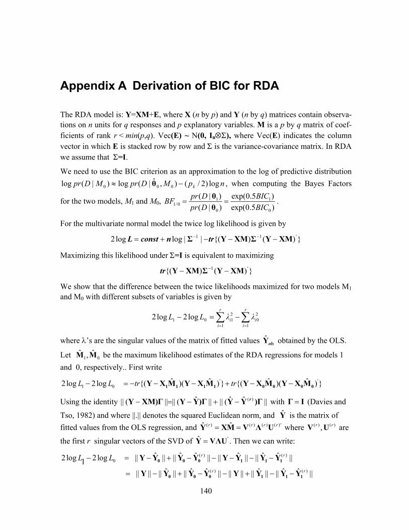
140

Appendix A Derivation of BIC for RDA

The RDA model is: Y=XM+E, where X (n by p) and Y (n by q) matrices contain observa-tions on n units for q responses and p explanatory variables. M is a p by q matrix of coef-ficients of rank r < min(p,q). Vec(E) ~ N(0, In⊗Σ), where Vec(E) indicates the column vector in which E is stacked row by row and Σ is the variance-covariance matrix. In RDA we assume that Σ=I.

We need to use the BIC criterion as an approximation to the log of predictive distribution npMDprMDpr k log)2/(),ˆ|(log)|(log 000 −≈ θ , when computing the Bayes Factors

for the two models, M1 and M0, 1 11/ 0

0 0

( | ) exp(0.5 )( | ) exp(0.5 )

pr D BICBFpr D BIC

= =θθ

.

For the multivariate normal model the twice log likelihood is given by

})(){(||loglog2 '11 XMYΣXMYΣ −−−+= −− trnconstL

Maximizing this likelihood under Σ=I is equivalent to maximizing

})(){( '1 XMYΣXMY −− −tr

We show that the difference between the twice likelihoods maximized for two models M1 and M0 with different subsets of variables is given by

∑∑==

−=−r

ii

r

ii λλLL

1

20

1

2101 log2log2

where λ’s are the singular values of the matrix of fitted values olsY obtained by the OLS.

Let 1 0ˆ ˆ,M M be the maximum likelihood estimates of the RDA regressions for models 1

and 0, respectively.. First write ' '

1 0ˆ ˆ ˆ ˆ2 log 2log {( )( ) } {( )( ) }L L tr tr− = − − − + − −1 1 1 1 0 0 0 0Y X M Y X M Y X M Y X M

Using the identity ||ˆˆ(||||ˆ(||||(|| )( )ΓYY)ΓYYXM)ΓY r−+−=− with =Γ I (Davies and

Tso, 1982) and where ||.|| denotes the squared Euclidean norm, and Y is the matrix of fitted values from the OLS regression, and ( ) ( ) ( ) ( ) 'ˆ ˆr r r r= =Y XM V Λ U where ( ) ( ),r rV U are

the first r singular vectors of the SVD of 'ˆ =Y VΛU . Then we can write: ( ) ( )

0

( ) ( )

ˆ ˆ ˆ ˆ ˆ ˆ2 log 2log || || || || || || || ||1ˆ ˆ ˆ ˆ ˆ ˆ || || || || || || || || || || || ||

r r

r r

L L− = − + − − − − −

= − + − − + − −

0 0 0 1 1 1

0 0 0 1 1 1

Y Y Y Y Y Y Y Y

Y Y Y Y Y Y Y Y

141

The second line is true because for the OLS regression, we can decompose the sum of squared residuals as follows (using the identity, '|| || ( )tr=A A A ).

'

'

1 1

ˆ ˆ ˆ|| || || || 2 ( ) || ||ˆ ˆ ˆ ˆ ˆ = || || 2 {( ) } 2 ( ' ) || ||

ˆˆ ˆ = || || ( ) || ||

ˆ || || || ||

q n

ij ij ijj i

tr

tr tr

y y y= =

− = − +

− − − +

− − −

= −

∑∑

Y Y Y Y Y Y

Y Y Y Y Y Y Y

Y Y

Y Y

Now by invoking the Eckart-Young (1936) theorem about low rank approximations of

rectangular matrices, we can write ( ) 2

1

ˆ ˆ|| ||q

ri

i rλ

= +

− = ∑Y Y where λi , i=1,..q are the singular

values of Y and therefore: ( ) ( )

1 0 1

2 2 2 21 1 0 0

1 1 1 1

ˆ ˆ ˆ ˆ ˆ ˆ2 log 2log || || || || (|| || || ||)

r r

q q q q

i i i ii i r i i r

L L

λ λ λ λ= = + = = +

− = − − − − −

= − − −

∑ ∑ ∑ ∑

1 1 0 0 0Y Y Y Y Y Y

2 21 0

1 1

( ) ( )

ˆ ˆ || || || ||

r r

i ii i

r r

λ λ= =

= −

= −

∑ ∑

1 0Y Y

as desired.

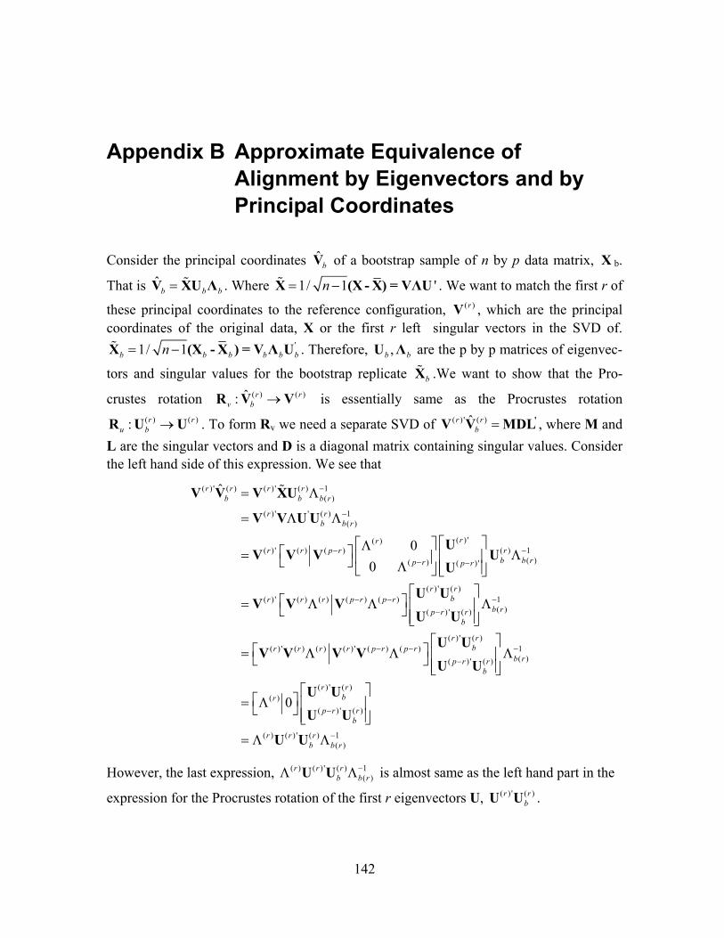
142

Appendix B Approximate Equivalence of Alignment by Eigenvectors and by Principal Coordinates

Consider the principal coordinates ˆbV of a bootstrap sample of n by p data matrix, X b.

That is ˆb b b=V XU Λ% . Where 1/ 1 'n= −X (X - X) = VΛU% . We want to match the first r of

these principal coordinates to the reference configuration, ( )rV , which are the principal coordinates of the original data, X or the first r left singular vectors in the SVD of.

'1/ 1b b b b b bn= −X (X - X ) = V Λ U% . Therefore, ,b bU Λ are the p by p matrices of eigenvec-

tors and singular values for the bootstrap replicate bX% .We want to show that the Pro-

crustes rotation ( ) ( )ˆ: r rv b →R V V is essentially same as the Procrustes rotation

( ) ( ): r ru b →R U U . To form Rv we need a separate SVD of ( ) ' ( )ˆr r

b = 'V V MDL , where M and L are the singular vectors and D is a diagonal matrix containing singular values. Consider the left hand side of this expression. We see that

( ) ' ( ) ( ) ' ( ) 1( )

( ) ' ' ( ) 1( )

( ) '( )( ) ' ( ) ( ) ( ) 1

( )( ) ( ) '

( ) ' ( )( ) ' ( ) ( ) ( ) ( ) 1

( )( ) ' ( )

( ) ' ( )

ˆ

00

r r r rb b b r

r rb b r

rrr r p r r

b b rp r p r

r rbr r r p r p r

b rp r rb

r r

−

−

− −− −

− − −−

= Λ

= Λ Λ

Λ = Λ Λ

= Λ Λ Λ

=

V V V XU

V V U U

UV V V U

U

U UV V V

U U

V V

%

( ) ' ( )( ) ( ) ' ( ) ( ) 1

( )( ) ' ( )

( ) ' ( )( )

( ) ' ( )

( ) ( ) ' ( ) 1( )

0

r rbr r p r p r

b rp r rb

r rbr

p r rb

r r rb b r

− − −

−

−

−

Λ Λ Λ

= Λ

= Λ Λ

U UV V

U U

U U

U U

U U

However, the last expression, ( ) ( ) ' ( ) 1( )

r r rb b r

−Λ ΛU U is almost same as the left hand part in the

expression for the Procrustes rotation of the first r eigenvectors U, ( ) ' ( )r rbU U .

143

Bibliography

Akaike, H. (1973). Information theory and an extension of the maximum likelihood prin-ciple. In 2nd International Symposium on Information Theory, eds. B. N. Petrov and F. Csaki, Budapest: academia Kiado, 267-281.

Anderson, T.W. (1951). Estimating linear restrictions on regression coefficients for multi-ple normal distributions. Annals of Mathematical Statistics, 29, 813-828

Antoniadis, A. and Fan, J. (2001). Regularization of wavelet approximations. JASA, 96:455, 939-962.

Atkinson, A.C. (1988). Transformations unmasked. Technometrics, 30, 311-318.

Banfield, J.D. and Raftery, A.E. (1993). Model based Gaussian and non Gaussian cluster-ing. Biometrics, 49, 803-821.

Bensmail, H., Celeux, G., Raftery, A.E. and Robert, C. (1997). Inference in model-based cluster analysis. Statistics and Computing, 7, 1-10.

Bensmail, H. and Meulman, J.J. (1998). MCMC Inference for model-based cluster analy-sis. In Advances in Data Science and Classification. Proceedings of the 6th Confer-ence of the International Federation of Classification Societies, Springer-Verlag (Ber-lin; New York), 191-196.

Breiman, L. (1996). Stacked regression. Machine Learning. 24, 49-64

Breiman, L. (1996a). Bagging predictors. Machine Learning. 24, 123-140

Breiman, L. (1992).The little bootstrap and other methods for dimensionality selection in regression: X-fixed prediction error. JASA, 87:419, 738-754.

Breiman, L. and Spector, P. (1992). Submodel selection and evaluation in regression. The X-random case. Int. Statist. Review, 60, 291-319.

Brown, P.J. and Vannucci, M. (1998). Multivariate Bayesian variable selection and pre-diction, J.R. Statist. Soc. B, 60:3, 627-641.

Buckland, S.T., Burnham, K.P. and Augustin, N.H. (1997). Model selection: an integral part of inference. Biometrics, 53:275-290.

Carlin. B.R. and Chib, S. (1995). Bayesian model choice via Markov chain Monte Carlo methods. J.R. Statist. Soc. B, 57:3, 473-484.

Chatfield, C (1995). Model uncertainty, data mining and statistical inference, J.R. Sta-tist.Soc. A, 158:3, 419-466

144

Chickering, D.W and Heckerman, D (2000). A comparison of scientific and engineering criteria for Bayesian model selection. Statistics and Computing, 10, 55-62.

Chipman, H. (1996). Bayesian variable selection with related predictors. The Canadian Journal of Statistics, 24:1, 17-36.

Chipman, H.A., George, E.I. and McCulloch, R.E. (1998). Bayesian CART model search. JASA. 93:443, 935-948.

Clarkson, D.B. (1979). Estimating the standard errors of rotated factor loadings by jack-knife. Phychometrika, 44, 3, 297-314

Clyde, M., DeSimone, H., and Parmigiani, G. (1996). Prediction via orthoganalized model mixing. JASA, 91:435, 1197-1208.

Clyde, M., Parmigiani, G. and Vidakovic, B. (1998). Multiple shrinkage and subset selec-tion in wavelets. Biometrika, 85, 391-402.

Clyde, M.A. (1999). Bayesian model averaging and model search strategies. In Bayesian Statistics 6, 157-185, Oxford University Press.

Clyde, M.A. (1999a). Discussion of Hoeting, J.A, Madigan, D, Raftery, A.E, Volinsky, C.T, Bayesian model averaging: a tutorial. Statistical Science, 14:4, 409-412.

Clyde, M.A. and George, E.I. (1999). Empirical Bayes estimation in wavelet nonparamet-ric regression. In Bayesian Inference in Wavelet-Based Models (P. Muller and B. Vi-dakovic, eds) 309-322. Springer, Berlin.

Cox, T.F. and Cox, M.A (1994). Multidimensional Scaling. Chapman & Hall, London

Davies, P.T. and Tso, K.S. (1982). Procedures for reduced-rank regression. Appl. Statist, 31:3, 244-255.

Draper, D. (1995). Assesment and propogation of model uncertainty (with discussion). J. Roy. Statist. Soc. B, 57, 45-70.

Eckart, C and Young, G. (1936). The approximation of one matrix by another of lower rank. Psychometrika, 1, 211-218.

Efron, B. (2000). The bootstrap and modern statistics. JASA. 95:452, 1293-1296.

Efron, B. and Gong, G. (1983). A leisurely look at the bootstrap, the jackknife, and cross-validation. American Statistician, 37, 36-48.

Efroymson, M.A. (1960). Multiple regression analysis. In Mathematical Methods for Digital Computers, eds. Ralston, A. and Wilf, H.S., Wiley, New York,191-203.

Fan, J. and Li, R. (1999). Variable selection via penalized likelihood, Technical report, Department of Statistics, UCLA

145

Foster, D.P. and George, E.I. (1994). The risk inflation criterion for multiple regression. The Annals of Statistics, 22, 1947-1975.

Fraley, C., Raftery, A.E. (1998). How many clusters? Which clustering method? Answers via model-based cluster analysis. Technical Report No. 329, Department of Statistics, University of Washington

Freedman, D.A., Navidi, W., Peters, S.C. (1986). On the impact of variable selection in fitting regression equations. In On model uncertainty and its statistical implications : proceedings of a workshop held in Groningen, the Netherlands, September 25-26, 1986 / Theo K. Dijkstra (ed.).

Furnival, G.M. and Wilson, R.W. (1974). Regression by leaps and bounds. Technomet-rics, 16, 499-511.

Gabriel, K.R. (1971). The biplot-graphic display of matrices with application to principal component analysis. Biometrika, 58, 453-67.

Gabriel, K.R. (1978). Least squares approximation of matrices by additive and multiplica-tive models. J.R. Statist. Soc. B , 187-196.

Gauch, H.G. (1982). Multivariate Analysis in Community Ecology. Cambridge University Press, Cambridge, 298.

Geisser, S. and Eddy, W.F. (1979). A predictive approach to model selection. JASA, 74:365, 153-160.

Gelfand, A.E. and Dey, D.K. (1994). Bayesian model choice: asymptotic and exact calcu-lations. J.R. Statist. Soc. B, 56:3, 501-514.

George, E.I. (1986). Minimax multiple shrinkage estimation. Annals of Statistics, 14, 188-205.

George, E.I. (1999). Discussion of “Model averaging and model search strategies” by M. Clyde. In Bayesian Statistics 6 (J.M. Bernardo, at al, eds), 157-185. University Press, Oxford.

George, E.I. (1999a). Discussion of Hoeting, J.A., Madigan, D., Raftery, A.E., Volinsky, C.T, Bayesian Model Averaging: a tutorial. Statistical Science, 14:4, 409-412.

George, E.I. (2000). The variable selection problem. JASA. 95:452, 1304-1308.

George, E.I. and McCulloch, R.R. (1993). Variable selection via Gibbs sampling. JASA, 88, 881-889.

George, E.I. and McCulloch, R.R. (1997). Approaches for Bayesian variable selection. Statist. Sinica 7, 339-373.

Geweke, J. (1996). Bayesian reduced rank regression in econometrics. Journal of econo-metrics, 75, 121-146.

146

Geweke, J. (1996). Variable selection and model comparison in regression. In Bayesian Statistics 5 (Edited by J.M. Bernardo, J.O. Berger, A.P. Dawid and A.F.M. Smith), 609-620.

Gower J.C. and Hand D.J. (1996) Biplots. Chapman and Hall, London.

Green, P.J. (1995). Reversible jump Markov chain Monte-Carlo computation and Bayes-ian model determination. Biometrika, 82, 711-732.

Greenacre, M.J. (1984). Theory and Application of Correspondence Analysis. Academic Press, London

Hastings, W.K. (1970). Monte Carlo sampling methods using Markov chains and their applications. Biometrika, 57:1, 97-109.

Hjorth, U. (1994). Computer Intensive Statistical Methods. Validation, Model Selection, and Bootstrap. Chapman & Hall, London.

Hoeting, J.A., Madigan, D., Raftery, A.E. and Volinsky, C.T. (1999). Bayesian model av-eraging: a tutorial (with discussion). Statistical Science, 14:4, 382-417.

Hoeting, J.A., Raftery, A.E., and Madigan, D. (1999a). Bayesian simultaneous variable and transformation selection in linear regression. Technical report 9905, Department of Statistics, Colorado State University, available at www.stat.colostate.edu

Hoeting, J.A., Raftery, A.E. and Madigan, D. (1996). A method for simultaneous variable selection and outlier identification in linear regression. Computational Statistics and Data Analysis, 22, 251-270. available at:

http://www.stat.washington.edu/raftery/Research/Mclust/mclust_papers.html

Ichikawa, M. and Konishi, S. (1995). Application of the bootstrap methods in factor analysis. Phychometrika, 60:1, 77-93

Izenman, A.J. (1975). Reduced-rank regression for the multivariate linear model. Journal of Multivariate Analysis, 5, 248-264

Jackson, J.,E. (1991). A user’s Guide to Principal Components. New York: Wiley & Sons

Johnson, D. E. (1998). Applied Multivariate Methods for Data Analysis. Brooks/ Cole Publishing Company, London.

Kass, R.E. and Raftery, A.E. (1995). Bayes Factors. JASA, 90, 773-795.

Kass, R.E. and Wasserman, L. (1995). A reference Bayesian test for nested hypotheses and its relationship to the Schwarz criterion. JASA, 90, 928-34.

Key, J.T, Pericchi, L.R. and Smith, A.F.M. (1999). Bayesian model choice: what and why? (with discussion). In Bayesian Statistics, 6, 343-370.

147

Krzanowski, W.J. and Radley, D. (1989). Nonparametric confidence and tolerance regions in canonical variate analysis. Biometrics, 45, 1163-1173

Krzanowski, W.J. (1989). On confidence regions in canonical variate analysis. Bio-metrika, 76:1, 107-116

Laud, P.W. and Ibrahim, J.G. (1995). Predictive model selection. J.R. Statist. Soc. B, 57:1, 247-262.

Laud, P.W. and Ibrahim, J.G. (1996). Predictive specification of prior model probabilities in variable selection. Biometrika, 83:2, 267-274.

Leamer, E.E. (1978). Specification Searches. Wiley, New York.

Legendre, P. and Legendre, L. (1998). Numerical ecology. Amsterdam

Lewis, S.M. and Raftery, A.E. (1997). Estimating Bayes factors via posterior simulation with the Laplace-Metropolis estimator. JASA, 92, 648-655

Lipkovich , I.A., Smith , E.P. and Ye, K. (2002). Evaluating the impact of environmental stressors on benthic microinvertebrate communities via Bayesian model averaging. In Case Studies in Bayesian Statistics 6th Workshop (to appear).

Lipkovich, I. and Smith, E.,P. (2001). Biplot and SVD macros for EXCEL. Journal of Statistical Software (under review).

Lynn, S. and McCulloch, C.E. (2000). Using principal component analysis and correspon-dence analysis for estimation in latent variable models. JASA, 95:450, 561-572.

Madigan, D., Gavrin, J. and Raftery, A.E. (1995). Eliciting prior information to enhance the predictive performance of Bayesian graphical models. Communications in statis-tics – Theory and Methods, 24, 2271-2292.

Madigan, D. and Raftery, A.E. (1994). Model selection and accounting for model uncer-tainty in graphical models using Occam’s window. JASA, 89:428, 1535-1546

Madigan, D. and York, J. (1995). Bayesian graphical models for discrete data. Int. Statist. Review. 63, 215-32.

Mallows, C.L. (1973). Some comments on Cp. Technometrics, 15, 661-676.

McLachlan, G.J. and Peel, D. (2000). Finite Mixture Models. Wiley, New York.

McQuarrie, A.D.R. and Tsai, C.L. (1998). Regression and Time Series. Model Selection. World Scientific, Singapore.

Meyer, D, R. and Wilkinson, R.G. (1998). Bayesian variable assessment. Communications in statistics – Theory and Methods. 27:11, 2675-2705

Miller, A. J. (1990). Subset Selection in Regression. Chapman and Hall, London.

148

Mitchell, T.J. and Beauchamp, J.J (1988). Bayesian variable selection in linear regression. JASA, 83:404, 1023-1036.

Noble, R. (2000). Multivariate Applications of Bayesian Model Averaging. PhD Disserta-tion, 2000, Virginia Polytechnic Institute.

Norton, S.B. (1999). Using Biological Monitoring Data to Distinguish Among Types of Stress in Streams of the Eastern Corn Belt Plains Ecoregion. Ph.D. thesis. George Mason University

O’Hagan, A. (1995). Fractional Bayes factors for model comparison (with discussion). Journal of the Royal Statisical Society, ser. B, 57:1, 99-138.

Pennel, R. (1972). Routinely computable confidence intervals for factor loadings using the “jackknife”. British journal of Mathematical and Statistical Phychology, 25, 107-114

Philips, R. and Guttman, I. (1998). A new criterion for variable selection. Statistics & Probability Letters 38, 11-19

Phillips, D.B. and Smith, A.F.M. (1995). Bayesian model comparison via jump diffusions. In Markov Chain Monte Carlo in Practice (edited by W.R. Gilks, S. Richardson and D.J. Spiegelhalter), 215-239. Chapman & Hall, London.

Pötscher, B.M. (1991). Effects of model selection on inference. Econometrics Theory, 7, 163-185.

Raftery, A.E. (1995) Bayesian model selection in social research (with discussion). In Marsden, P.V., editor, Sociological Methodology, 111-195. Blackwells Publishers, Cambridge, Mass

Raftery, A.E. (1996). Approximate Bayes factors and accounting for model uncertainty in generalized linear models. Biometrika, 83, 251-266.

Raftery, A.E., Madigan, D. and Hoeting, J.A. (1997). Bayesian model averaging for linear regression models. JASA, 92:437, 179-191.

Rao, C.R. (1964). The use and interpretation of principal components analysis in applied research. Sankhya A, 26, 329-358.

Reinsel, G.C. and Velu, R.P. (1998). Multivariate Reduced-Rank Regression. Springer-Verlag, New York.

Reynoldson, T.B., Day, K.E. and T. Pascoe. (2000). The development of the BEAST: a predictive approach for assessing sediment quality in the North American Great Lakes. In Assessing the biological quality of freshwaters. RIVPACS and other tech-niques, (editors J.F. Wright, D.W. Sutcliffe and M.T. Furse). Freshwater Biological Association, Ambleside, UK. Chapter 11, 165-180.

149

Reynoldson, T. B. and Day, K.E. (1998). Biological Guidelines for the Assessment of Sediment Quality in the Laurentian Great Lakes. NWRI Report No. 98-232. 119 pages + appendices.

Rubin, D.B. (1987). Multiple Imputation for Nonresponse in Surveys. J. Wiley & Sons, New York.

Schafer, J.L. (1997). Analysis of Incomplete Multivariate Data. Chapman and Hall, Lon-don.

Schwarz, G. (1978). Estimating the dimension of a model. The Annals of Statistics, 6:2, 461-464.

Shao, J. (1997). An asymptotic theory for linear model selection. Statistica Sinica, 7, 221-264.

Shao, J. (1996). Bootstrap model selection. JASA, 91:434, 655-665.

Shively, S., Kohn, R. and Wood, S. (1999) Variable selection and function estimation in additive nonparametric regression using a data based prior (with discussion). JASA, 94:447, 777-806.

Smith, A.F.M. and Roberts, G.O. (1993). Bayesian computation via the Gibbs sampler and related Markov chain Monte Carlo methods. J.R. Statist. Soc. B, 55:1, 3-23.

Smith, A.F.M. and Spiegelhalter, D.J. (1980). Bayes factors as choice criteria for linear models. J.R. Statist. Soc. B, 42:2, 213-220.

Smith, M. and Kohn, R. (1996). Nonparametric regression using Bayesian variable selec-tion. Journal of Econometrics, 75, 317-343.

Tanner, M.A. and Wong, W.H. (1987). The calculation of posterior distributions by data augmentation. JASA, 82:398, 528-540.

ter Braak, C.J.F (1986). Canonical correspondence analysis: A new eigenvector technique for multivariate direct gradient analysis. Ecology, 67:5, 1167-1179.

ter Braak, C.J.F. (1985). Correspondence analysis of incidence and abundance data: prop-erties in terms of a unimodal model. Biometrics, 41, 859-873.

ter Braak, C.J.F.(1992). Permutation versus bootstrap significance tests in multiple regres-sion and ANOVA. In Jokel K.H., Rothe, G. and Sendler, W. (eds), Bootstrapping and Related Techniques, Springer Verlag, Berlin, 79-85

ter Braak, C.J.F.(1994). Biplots in reduced-rank regression. Biom. J. 36:8, 983-1003

ter Braak, C.J.F. and Prentice, I.C. (1988). A theory of gradient analysis. Advances in eco-logical research, 18, 272-317.

150

ter Braak, C.J.F. and Verdonschot, P.F.M. (1995). Canonical correspondence analysis and related multivariate methods in aquatic ecology. Aquatic Sciences. 57:3, 255-289.

Thisted, R.A. (1988). Elements of Statistical Computing. Chapman and Hall, London.

Tso, K.S. (1981). Reduced-rank regression and canonical analysis. J.R. Statist. Soc. B, 43:2, 183-189.

Tyler, D.E. (1981). Asymptotic inference for eigenvectors. The Annals of Statistics, 9, 4, 725-736

Van der Leeden, R. (1990). Reduced Rank Regression With Structured Residuals. DSWO Press, Leiden.

Volinsky, C., Madigan, D., Raftery, A.E. and Kronmal, R.A. (1997). Bayesian model av-eraging in proportional hazard models: assessing the risk of a stroke. Applied Statis-tics, 46:4, 433-448.

Wedel, M. and Kamakura, W.A. (1999). Market Segmentation, Methodological and Con-ceptual Foundation. Dordrecht: Kluwer, 2nd edition.

Weinberg, S.L. and Carroll, J.D. (1984). Confidence regions for INDSCAL using the jackknife and bootstrap techniques. Psychometrica, 49:4, 475-491

151

Ilya A. Lipkovich

Education

Virginia Polytechnic Institute and State University, Blacksburg, Virginia, Department of Statistics. Degree: doctor of Philosophy in Applied Statistics. GPA 4.0. Dissertation topic: Bayesian Model Averaging in Multivariate Ecological Models. Graduation date: May 2002

8/ 98 – 4/ 02

University of Delaware, Department of Mathematical Sciences, Newark, Delaware. Degree: Master of Science in Applied Statistics. GPA 3.9. May 1998

9/ 95 – 6/ 98

Almaty Institute of National Economy. Almaty, Kazakhstan, Department of Statistics. Degree: equivalent to Bachelor of Science in statistics and economics. GPA 4.0. May 1985.

9/ 81 – 6/ 85

Experience

Senior Statistician at Eli Lilly and Company, Indianapolis, Indiana. De-signs and analyzes projects in the phase IV clinical areas.

to start 4 / 02

Instructor at Virginia Tech, Department of Statistics, Blacksburg, Vir-ginia. Teaching an introductory Biological Statistics class, developed lec-ture notes, prepared tests and quizzes. The course materials are available at http://filebox.vt.edu/users/ilipkovi/

9/01–1/02

Graduate Assistant at Virginia Tech, Department of Statistics, Blacks-burg, Virginia. Worked on a grant supported project (developed statistical software in VBA, performed analysis of ecological data).

Consultant at Statistics department consulting center. Consulted with non-statistics faculty and graduate students. Analyses included regression, multivariate methods, non-parametric methods, time series. Helped clients design and analyze experiments

9/ 98 – 4/02

Intern at DuPont company, Quality Management and Technology Cen-ter, Wilmington, Delaware. Worked on various projects involving design, analysis of experiments, and observational data analysis. Developed a set of tools for comprehensive validation of statistical software. Developed software for data analysis in SAS and Visual Basic, which included VBA macros for analysis of toxicological dose-response experiments, statistical quality control and analysis of factorial designs

8/ 97 – 6/ 98

152

Consultant at Statistical Laboratory, University of Delaware, Depart-ment of Mathematical Sciences. Newark, Delaware. Consulted with clients from various departments of UD, provided information on appropriate sta-tistical methods and interpretation of results, analyzed their data using SAS and SPSS, made presentations at weekly meetings. Was responsible for a special survey project

9/ 96 – 5/ 97

Consultant, World Bank, Economic Development Institute, Washington, DC. Developed a general purpose statistical software (INFRISK) for risk analysis of infrastructure projects based on Monte Carlo simulation (Visual Basic for Applications). Developed econometric models for panel data on infrastructure bonds (generalized estimating equations, survival analysis)

6–8/ 99; 6–8/98;

6– 8/ 97

Consultant, World Bank, Washington, DC. Designed and analyzed data from a comprehensive statistical survey for the social assessment of a large-scale irrigation project in Kazakhstan

6–8/ 96

Teaching Assistant, University of Delaware, Department of Mathematical Sciences. Newark, DE. Was responsible for running lab sessions in intro-ductory statistical courses, designed homework assignments and tests.

9/ 95 – 9/ 96

Instructor, University of Delaware, Department of Mathematical Sci-ences.

Taught an introductory course in business statistics. Developed lectures and tests

1-2/ 96

Consultant, World Bank, Almaty, Kazakhstan. Taught courses in statisti-cal modeling of housing market data at several World Bank seminars in Kazakhstan and Republics of Central Asia

4–7/ 95

Data analyst and software expert, International City/County Manage-ment Association, Almaty, Kazakhstan. Analyzed survey data, developed statistical models for the real estate appraisal; developed simulation models for housing allowances program, wrote reports.

1/ 94 – 3/ 95

Statistician/Programmer, StatEx Ltd., Almaty, Kazakhstan. Developed general-purpose statistical software using Turbo Pascal and C. Worked with a small team of statisticians and programmers. The statistical soft-ware developed (STATEX and QUESTIONNARIE) were used in many companies and research firms in Russia and Kazakhstan.

1/ 90 – 12/ 93

Data analyst and research assistant, Almaty Institute of National Econ-omy, Almaty, Kazakhstan. Analyzed data using multivariate methods, per-formed Monte Carlo simulations, maintained and enhanced a large FOR-TRAN library of statistical programs.

5/ 87 – 12/ 89

Economist/Statistician, The Statistical Committee of the Republic of Ka-zakhstan.

8/ 85 – 11/ 85

bayesian model averaging and variable selection in multivariate ... · bayesian model averaging and...

Documents