Department of Physics and Astronomy, University of Canterbury,Private Bag 4800, Christchurch, New Zealand

Averaging the Inhomogeneous Universe

YAO Hui

MAPH480 Project 2006

Supervisor: Dr David L. WILTSHIRE

Abstract

We re-formulate and examine T. Buchert’s recent averaging scheme for scalars in cosmolog-ical applications of general relativity. The equation thus obtained can be used to describethe averaged quantities of an arbitrary inhomogeneous co-moving region and show the im-portance of back-reaction.

We also study the use of information theory in this averaging framework. Original exten-sions are mainly made along two lines: the information of inhomogeneity for different scalesare compared; the possibility of use of Shannon’s entropy in inhomogeneous cosmology areinvestigated. We also discuss the non-locality of gravitational energy in inhomogeneouscosmology.

Examples of cosmological solutions of Buchert’s averaging scheme are studied.

Contents

1 Introduction 1

2 The Averaging Procedure 5

2.1 The 3+1 decomposition and Einstein’s equations . . . . . . . . . . . . . . . . 5

2.2 Averaging Einstein’s equations . . . . . . . . . . . . . . . . . . . . . . . . . . 6

2.3 The cosmic quartet . . . . . . . . . . . . . . . . . . . . . . . . . . . . . . . . 8

3 The Information of Cosmological Inhomogeneity 10

3.1 The relative entropy in cosmology . . . . . . . . . . . . . . . . . . . . . . . . 10

3.2 The component information and the structure information . . . . . . . . . . 12

3.3 The effective entropy in cosmology . . . . . . . . . . . . . . . . . . . . . . . 14

3.4 Non-locality of Gravitational Energy . . . . . . . . . . . . . . . . . . . . . . 16

4 Examples 20

4.1 Globally static Universe . . . . . . . . . . . . . . . . . . . . . . . . . . . . . 20

4.2 Globally stationary Universe . . . . . . . . . . . . . . . . . . . . . . . . . . . 21

4.3 The example of an accelerating Universe . . . . . . . . . . . . . . . . . . . . 23

5 Conclusion 24

Acknowledgments 26

Bibliography 27

A Notation and Conventions 29

B Details of calculation for section 3.4 30

iii

Chapter 1

Introduction

The main direction of modern fundamental physics is to conquer the unknown in the two

extreme scales. On the one hand, pursuits are being continued to understand the final

building blocks of the Universe and the nature of spacetime at Planck scale. On the other, it

is the modernisation of cosmology—the study of the Universe at the large scale—that made

these two efforts symmetric and, more importantly, connected, as the two extreme ends will

turn out to be the one: unified laws of physics, governing all.

This effort is a manifestation of belief in the simplicity of nature. However, caution has

also been exerted. Einstein said: “Everything should be made as simple as possible, but

not simpler.1” Following in this spirit, we study cosmology—the simple laws describing the

most complex object; in particular, we study inhomogeneous cosmology, the class of theories

which are far more complex than the simple homogeneous standard models; even more par-

ticularly we will study the averaging procedure in inhomogeneous cosmology, the powerful

and profound technique which enables us to extract simple properties from a complex system

and to examine the “Universe seen at different scales”. We therefore, before our formal ex-

position, ask three questions: What is the current status of cosmology? Why inhomogeneous

cosmology? Why averaging in inhomogeneous cosmology?

What is the current status of cosmology?

The advancement of modern cosmology is brought forth by technology and the availability

of massive flow of astronomical data, especially those from Sloan Digital Sky Survey(SDSS),

the Hubble telescope, the Chandra telescope and WMAP. Most cosmologists would agree

on that we are entering an era of “precision cosmology”, when data collected will be made

more and more precise to put constraint on cosmological parameters, cosmological models

and new physics proposed.

Although being in an optimistic situation, we need to emphasize that cosmology is a very

special subject and therefore has its special difficulties [2]. Its object of study, the Universe

as a whole together with its role as the background for all the rest of physics and science,

challenges both physicists and philosophers; philosophical preferences strongly influence the

resulting understanding and choices of models studied. Fashion or sociology in science could

be a tremendous negative force in studies of theory and investments of experiments, and

analysis of data is inevitably model-dependent. We are limited in our ability to observe both

1As quoted in [1].

1

the very distant regions and the very early times, and limited in our ability to test physics in

a direct manner over the large scale and to test high energy physics relevant at the earliest

epochs. It is very impressive to see how the new version of the standard model, the ΛCDM

model, is able to explain and predict wide classes of independent phenomena, especially the

newly released WMAP data [3]. However, “many commonly discussed elements of cosmology

still are on dangerous ground” [4]. Here we discuss some conceptual problems [5] of modern

cosmology which are of particular interest to our later discussion.

1) Gravitational energy problem. In FLRW model, conservation of energy-momentum

in General Relativity(GR) is equivalent to dE = −p dV for an arbitrary co-movig region.

This of course should be directly interpreted as the first law of thermodynamics for fluid

with no heat transfer. As long as the fluid is not ideal dust with zero pressure, we see that

an expanding universe would lead to a decrease of matter energy. We will discuss these

problems in section 3.4.

2) Dark energy problem. In the past decade, observations of the luminosity-distance of

TypeIA supernovae have been interpreted within FLRW model as that the scale factor of the

Universe must have a positive second order time derivative (“the Universe is accelerating”).

Together with WMAP and other independent observations, the best-fit parameters indicate

that 75% of the energy content of the Universe must be in a mysterious form of non-luminous,

non-gravitationally-clumping, negative pressure fluid, known as “dark energy”. The nature

of dark energy so far still lacks physical basis.

3) Hubble–de Vaucouleurs paradox. Hubble’s discovery that the redshift of a galaxy

is proportional to its distance is one of the cornerstones of the standard model. According

to modern observations, a linear Hubble’s law is well established starting from scales about

1.5 to 2 Mpc. This is usually understood to imply a homogeneous Universe. Hubble’s

law is directly deducible from the FLRW model, but the converse is not true. In fact, an

inhomogeneous matter distribution is observed from the scale of the atoms up to at least

the scales of superclusters and voids. Sandage et al. [6] were the first to note the puzzling

co-existence of the linear Hubble’s law and the (at least local) inhomogeneity. Although

their original paper was arguing against de Vaucouleurs’ hierarchy Universe based on the

linearity of Hubble’s law, it remains a great challenge to explain the co-existence of these two

independent universal aspects and it is indeed a crucial task to solve in modern cosmology.

Why inhomogeneous cosmology?

The central idea of inhomogeneous cosmology is to emphasize the importance of cosmo-

logical structures. There are three aspects of these:

• To study classes of (exact or non-exact) solutions of Einstein’s equations as cosmo-

logical models without the assumptions of homogeneity and isotropy. These problems

should not be categorised merely as pure mathematical problems. In fact, exact inho-

mogeneous solutions can describe several features of the Universe in agreement with

observations, especially the existence of voids [6].

• To investigate the effects of global expansion on local physics.

• To study effects of local inhomogeneous structures on the dynamics of global geom-

etry. Termed “back-reaction”, this aspect of cosmology is attracting more and more

2

researchers currently. This is encouraged by the increasing evidence of inhomogene-

ity and motivated as alternative solutions to the dark energy problem. We will be

particularly interested in this last aspect.

One particular interesting idea is the modern version of the hierarchy Universe—fractal

cosmology. Fractals are ubiquitous in Nature; should cosmology be an exception? Fractal

cosmology is based on modern observation. Pietronero [8], using statistical methods, argues

that in the various surveys galaxy counts are proportional to rD at least up to 20Mpc, where

r is radial distance and D ≈ 2 is fractal dimension. Recently it was further argued that the

above result is consistent with SDSS [9]. Fractal cosmology is based on a weaker interpre-

tation of the Copernican principle—the “conditional cosmological principle” formulated by

Mandelbrot. A concrete formulation of these ideas in GR is very difficult. Examples of these

efforts are [10], [11]. The validity of fractal cosmology remains an interesting open question.

Why averaging in inhomogeneous cosmology?

Any mathematical description of a physical system depends on an averaging scale charac-

terizing the nature of the model [12]. This scale is usually taken as understood and therefore

hidden from the model, but it is one crucial element of the model. For example, a fluid

continuum is an averaged concept over a scale which must be large enough such that the

property of each individual molecule can be neglected, yet small enough such that spatial

gradients of properties under interest are well represented and not smoothed out. Similar

concerns were also pointed out by Tolman [13] back in the 1930s: although most cosmological

quantities are assumed to be smooth functions which assign an exact value to each point of

the spacetime, they are really macroscopically and phenomenologically identified. It is the

(spacetime) averaged quantity that have direct observational status and physical meanings

[14].

Applications of general relativity in cosmology usually start from implicitly assuming the

validity of the theory at the largest scale, whereas GR is indeed only tested directly at the

solar scale. The problem lies in the fact that GR is not scale invariant! Suppose we have some

well defined averaging procedure 〈 〉1 over some scale L1 for tensors and assume GR is valid in

a direct manner over L1, by which we mean the following: (i) calculate the Einstein’s tensor

G from the L1-averaged metric tensor 〈g〉1 to obtain G(〈g〉1); (ii) determine the L1-averaged

energy-momentum 〈T〉1; (iii) then Einstein’s equations tell us that G(〈g〉1) = κ 〈T〉1, where

κ is a universal constant. In practice, L1 is implicitly assumed and 〈 〉1 is normally dropped.

Einstein’s equation is then commonly written as G(g) = κT. However, at some larger scale

L2, we need to average the above equation to obtain: 〈G(〈g〉1)〉2 = κ 〈〈T〉1〉2. If we pay

attention to the fact that G is a function of 〈g〉1 and its first/second order derivatives, we

see that the above valid equation is very different from G(〈〈g〉1〉2) = κ 〈〈T〉1〉2. The use of

Einstein’s equation implicitly requires an averaging scale L1; its direct use over some scale

L1 is not in general mathematically compatible with its direct use over some other scale L2.

As pointed out by Zalaletinov [15], we can either interpret GR macroscopically and

derive GR itself from some microscopic equations describing systems at smaller scales, or we

can interpret GR microscopically and derive the averaged macroscopic equations describing

physical systems at larger scales. The latter interpretation is inevitable in the study of

cosmology, since whatever scale we start with, we will need the averaged equations to describe

3

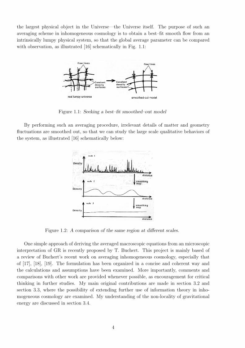
the largest physical object in the Universe—the Universe itself. The purpose of such an

averaging scheme in inhomogeneous cosmology is to obtain a best–fit smooth flow from an

intrinsically lumpy physical system, so that the global average parameter can be compared

with observation, as illustrated [16] schematically in Fig. 1.1:

Figure 1.1: Seeking a best–fit smoothed–out model

By performing such an averaging procedure, irrelevant details of matter and geometry

fluctuations are smoothed out, so that we can study the large scale qualitative behaviors of

the system, as illustrated [16] schematically below:

Figure 1.2: A comparison of the same region at different scales.

One simple approach of deriving the averaged macroscopic equations from an microscopic

interpretation of GR is recently proposed by T. Buchert. This project is mainly based of

a review of Buchert’s recent work on averaging inhomogeneous cosmology, especially that

of [17], [18], [19]. The formulation has been organized in a concise and coherent way and

the calculations and assumptions have been examined. More importantly, comments and

comparisons with other work are provided whenever possible, as encouragement for critical

thinking in further studies. My main original contributions are made in section 3.2 and

section 3.3, where the possibility of extending further use of information theory in inho-

mogeneous cosmology are examined. My understanding of the non-locality of gravitational

energy are discussed in section 3.4.

4

Chapter 2

The Averaging Procedure

In this chapter we will study the averaging procedure recently proposed by Buchert [17].

Through out this paper, we will restrict ourselves with irrotational dust continuum, that is,

cosmic fluid with negligible pressure and vorticity. For a similar averaging method covering

general perfect fluid, see [20]. For an alternative averaging procedure, see [14]. For a general

review on the early work of averaging problem prior to 1997, see chapter 8 of [7].

2.1 The 3+1 decomposition and Einstein’s equations

We start with the 3+1 splitting of the 4-dimensional manifold of spacetime of the Universe

M into one-parameter foliations of spacelike hypersurfaces Σt, labelled by global time coordi-

nate1 t. This is possible in general if M is globally hyperbolic. For such a choice of foliation,

it is always possible to choose Gaussian normal coordinates2, i.e. ds2 = −dt2 + gijdxidxj.

The parameter t is the proper time of observers co-moving with the cosmic fluid, for whom

∂txi = 0. The trajectories of fluid elements follow timelike geodesics everywhere orthogonal

to Σt, with unit tangent 4-vector ua = (1, 0, 0, 0), ua = (−1, 0, 0, 0).

For this choice of foliation, we define the extrinsic curvature of Σt with respect to M:

Kij ≡ −ui;j = Γ0ij u0 = −1

2gij,0 (2.1)

For this specific choice of coordinates, Einstein’s equations with a dust source and a

cosmological constant Gab = 8πρuaub − Λgab are equivalent to (see, e.g., section II of [23]):

1

2(R + K2 −Ki

jKji) = 8πGρ + Λ (2.2)

Kij||i −K,j = 0 (2.3)

Kij,0 = KKi

j + Rij − (4πGρ + Λ)δi

j (2.4)

where R = Rii is the Ricci scalar corresponding to the metric gij, K = Ki

i, and indices are

lowered/raised with respect to gij.

1See section 2.1 of [21] and reference therein, or section 21.4, 21.5 of [22] for further discussion.2This will be our working assumption, which is also the assumption of FLRW model and various other

models. But it introduces certain physical and geometrical restrictions, especially the existence of a globalproper time, which should be investigated more carefully.

5

For irrotational dust, we decompose the extrinsic curvature as: −Kij = ui;j ≡ σij + 13θgij,

where θ ≡ ui;i is the expansion rate, and σij is the shear tensor which is easily seen to be

trace-free and symmetric. We define the rate of shear σ correspondingly as 12σi

jσji. (See,

e.g., chapter 22 of [22]. Note the four-acceleration: uaub;a vanishes.)

With the above notation, (2.1),(2.2),(2.3) now read

gij,0 = 2σij +2

3θgij (2.5)

1

2R +

1

3θ2 − σ2 = 8πGρ + Λ (2.6)

σij||i −

2

3θ,j = 0 (2.7)

where all quantities depend on 4-coordinates (xa). We will call (2.6) the Friedmann equation.

Contracting i, j of (2.4), with the help of (2.6), we have the following Raychaudhuri equation:

θ +1

3θ2 + 2σ2 + 4πGρ− Λ = 0 (2.8)

Using again (2.6) and (2.8), equation (2.4) now reads

σij,0 + θσi

j + Rij −

1

3Rδi

j = 0 (2.9)

Finally, the conservation of energy equation (ρuaub);a = 0 , when contracted with ub,

gives:

ρ = Kρ = −θρ (2.10)

We also denote J =√

det(gij), then we have

J =1

2gikgki,0J = θJ (2.11)

It then follows from (2.10) and (2.11)that:

ρ(t, xi) = ρ(t0, xi)J(t0, x

i)(J(t, xi))−1 (2.12)

2.2 Averaging Einstein’s equations

We define the spatial averaging of a scalar field Ψ(t, xi) over a compact portion D of spacelike

hypersurface Σt as the following linear operation:

Ψ(t, xi) →⟨Ψ(t, xi)

⟩D≡ 1

VD

∫D

Ψ(t, xi)dV (2.13)

where we have used dV ≡ Jd3x for clarity and VD ≡∫

DdV is the integrated proper volume.

We therefore obtain the averaged covariant (with respect to spatial coordinates transfor-

mation) scalar field if we assign each point of D with the value 〈Ψ(t, xi)〉D indistinguishably.

However, such obtained “coarse-grained” field would not be globally smooth, and would

depend on arbitrary choice of division of Σt into a collection of averaging regions. Alterna-

tively, we can proceed as following: for some t, at each point xi ∈ Σt, we assign an unique

6

co-moving averaging region Dxi with xi in its interior. We define the value of the averaged

field at xi to be:

〈Ψ〉 (xi, t) ≡ 1

Vxi

∫Dxi

Ψ(t, xi) dV

where again Vxi is the proper volume of the co-moving region at time t. In order to get an

unique, covariant, globally smooth field, we would have to require a way of “coordinating”

averaging regions. For further pursuit along this direction, see cite15. However, from now

on, unless otherwise clearly stated, we will constrain ourselves with the study of a given fixed

co-moving averaging region. We emphasise that the averaged quantity is domain dependent,

even if when subscript “D” is dropped for convenience.

We also remark that the averaging defined above has physical meaning most transparent

if our primary concern of Ψ is energy density ρ. But for an arbitrary scalar field, the physical

meaning of this procedure is not as clear. For example, for a scalar field of temperature, it

is not clear that the volume averaging represents “the averaged temperature”. For energy

density field, the local form of conservation of energy (2.12) is equivalent to

M ≡∫

ρ dV = 〈ρ〉V = const. (2.14)

However, we make the warning that the total matter energy for an isolated co-moving region

is not a constant in general. See section 3.4 for further discussion.

In analogy to the standard cosmology, we define an effective scale factor

a(t) = (V (t)

V0

)13 (2.15)

where a subscript ”0” denotes the value at some initial time t0.

We similarly define effective Hubble function:

H(t) =a

a(2.16)

and effective deceleration parameter :

q(t) = − a

a

1

H2(2.17)

These quantities of course reduce back to the standard definition when we have, hypotheti-

cally, a homogeneous energy distribution.

With the above notation, the averaged expansion rate has a transparent meaning:

〈θ〉 =V

V= 3

a

a= 3H (2.18)

The important commutation rule then follows naturally from (2.11),(2.18):

∂t 〈Ψ〉 − 〈∂tΨ〉 = 〈Ψ θ〉 − 〈Ψ〉〈θ〉 = 〈Ψ δθ〉 = 〈θ δΨ〉 = 〈δΨ δθ〉 (2.19)

where δΨ = Ψ − 〈Ψ〉 and δθ = θ − 〈θ〉. The key statement of (2.19) is that the operations

of spatial averaging and time evolution do not commute.

7

For Ψ = ρ, this gives:

∂t 〈ρ〉 = −〈ρ〉〈θ〉 (2.20)

which should be compared with (2.10).

We next obtain two important results. The averaged Friedmann equation is the spatial

averaging of (2.6):

3 (a

a)2 − 8πG

M

V0a3+

1

2〈R〉 − Λ = −Q

2(2.21)

where

Q =2

3(⟨θ2

⟩− 〈θ〉2)− 2

⟨σ2

⟩=

2

3

⟨(θ − 〈θ〉)2

⟩− 2

⟨σ2

⟩(2.22)

is the back-reaction term which represents the global effect of local inhomogeneity. Averaging

(2.8), using (2.18) and (2.19), we obtain the averaged Raychaudhuri equation:

3a

a+ 4πG

M

V0a3− Λ = Q (2.23)

Equations (2.21) and (2.23) as well as their special forms in particular cosmology of chapter

4 will be referred simply as the averaged equations for convenience.

If we treat M, V0 and Λ as parameters to be determined observationally, then (2.21) and

(2.23) form a system of two ordinary differential equations with three unknowns. Unless we

introduce extra simplifying assumptions, this system can not be solved.

We end this section by stating the following necessary integrability condition, obtained

by differentiating (2.21) and using (2.23):

∂tQ+ 6a

aQ+ ∂t 〈R〉+ 2

a

a〈R〉 = 0 (2.24)

or equivalently:1

a6∂t(Qa6) +

1

a2∂t(〈R〉 a2) = 0 (2.25)

which shows that the averaged intrinsic curvature 〈R〉 and the averaged extrinsic curvature

(encoded in Q) are dynamically coupled.

2.3 The cosmic quartet

In this section, we draw further analogies to homogeneous cosmology and study the features

of averaged equations for a fixed co-moving region.

We start by interpreting Q, 〈R〉 , Λ as effective sources of gravitation, and define the

corresponding effective energy density as:

ρQ = − 1

16πGQ ρ〈R〉 = − 1

16πG〈R〉 ρΛ =

1

8πGΛ (2.26)

We also define the total energy density and the critical density as:

ρtot = 〈ρ〉+ ρQ + ρ〈R〉 + ρΛ, ρcri =3H2

8πG(2.27)

8

We emphasize that although formally identical, the critical density defined here in general

does not play the same role as the critical density in the standard model, i.e., it is not the

borderline between a closed Universe and an open Universe.

We continue to define the corresponding effective pressure respectively as:

pQ = ρQ = − 1

16πGQ p〈R〉 = −1

3ρ〈R〉 =

1

48πG〈R〉 pΛ = −ρΛ = − 1

8πGΛ

(2.28)

ptot = pQ + p〈R〉 + pΛ = − 1

16πGQ+

1

48πG〈R〉 − 1

8πGΛ (2.29)

The significance of the above formalism lies almost entirely in the following simple and

physically clear re-expression of (2.21),(2.23),(2.24):

3 (a

a)2 = 8πG ρtot (2.30)

3a

a= −4πG (ρtot + 3 ptot) (2.31)

ρtot + 3H(ρtot + ptot) = 0 (2.32)

Equations (2.30),(2.31) of course are just normal Friedmann equation and Raychaudhuri

equation with ordinary homogeneous fluid density replaced by our effective density which

takes into consideration of inhomogeneity structure.

However, we remark that this interpretation has only limited use. Especially, ρtotV for

an isolated fixed co-moving region generally is not a constant with respect to time. This is

manifest from differentiating ρtotV and comparing to (2.25). There is no physical reason to

view the change of ρtotV as transference to gravitational energy. In particular we note that

the term ρ〈R〉 and ρQ already represent gravitational structure. See section 3.4 for further

discussion.

For completeness of the analogy, we now further define the corresponding effective density

parameter respectively as following:

Ωm =〈ρ〉ρcri

=8πGM

3V0a3H2ΩQ =

ρQρcri

= − Q6H2

Ω〈R〉 =ρ〈R〉ρcri

= − 〈R〉6H2

ΩΛ =ρΛ

ρcri

=Λ

3H2(2.33)

and therefore (2.21) is equivalent to a form Buchert [18] dubs the cosmic quartet :

Ωm + ΩQ + Ω〈R〉 + ΩΛ = 1 (2.34)

Similar to the remark following (2.23), the system of ordinary differential equations

(2.30),(2.31) could be solved if a cosmic equation of state is given in the form ptot =

ptot(ρtot, a). Therefore questions related to the evolution of the inhomogeneous Universe

could be “reduced” to the problem of finding a cosmic state on a given spatial scale. Al-

though formally similar to the situation in the standard cosmology, here the equation of

state is dynamical and depends on the details of the evolution.

9

Chapter 3

The Information of CosmologicalInhomogeneity

Before we move on to investigate the interesting examples of the solutions to the system

of equations obtained in chapter 2, in this chapter we will use the language of information

theory to study the spatially averaged inhomogeneous Universe. In section 3.1 we review the

work of Hosoya et al. [18]. In section 3.2 we point out one important feature of the quantity

proposed in [18]. In section 3.3, we suggest another possible definition of [18].

3.1 The relative entropy in cosmology

In standard information theory, the well known relative entropy or Kullback-Leibler infor-

mation S is defined [1] as

S(p||q) =∑

pi ln(pi

qi

) for discrete random variable, or

S(p||q) =

∫p(x) ln(

p(x)

q(x)) dx for continuous random variable (3.1)

where p, q are two different probability distributions of the same random variable. This

is a quantity measuring the inefficiency of assuming the distribution is q when the “true”

distribution is p, or a measure of the “distance” between two different distributions. (The

word “distance” is used in a very limited sense, since this quantity is not generally symmetric

in p, q, let alone satisfying the triangle inequality.)

Application of this concept in inhomogeneous cosmology starts from identifying the prob-

ability distribution of p and q as energy density distribution of ρ and 〈ρ〉 respectively:

SD =

∫D

ρ ln(ρ

〈ρ〉D) dV (3.2)

We have dropped the explicit distribution dependence of SD since they are implicitly assumed

to be ρ, 〈ρ〉D without chances of confusion, but we have put subscript D to emphasize its

regional dependence, for reasons to become clearer in the next section. This quantity is

strictly positive, unless in the case of a homogeneous distribution ρ = 〈ρ〉D it vanishes.

Similar to the original use of relative entropy in information theory, we could view (3.2) as

10

an estimate of the inefficiency of assuming a homogeneous region when the true distribution

is inhomogeneous, or the degree of cosmological inhomogeneity.

Comparing with the standard index of inhomogeneity in cosmology:

(∆ρ)2

〈ρ〉D=〈ρ2〉 − 〈ρ〉2

〈ρ〉D(3.3)

we see the relative entropy is at least complementary. As pointed out in [18], (3.2) and (3.3)

are both members of a one-parameter family of inhomogeneity measures, the Tsallis relative

entropy, defined by :

Fα =〈ρ〉Dα

( ⟨(

ρ

〈ρ〉D)α+1

⟩D

− 1

)(3.4)

with α as a real parameter. When α = 1, (3.4) reduces to (3.3) and when α → 0, the limit

is (3.2). However, the relative entropy we adopted as in (3.2) is the only quantity satisfies

the following remarkable property: differentiating (3.2) and use (2.19), we have:

SD

VD

= 〈∂tρ〉D − ∂t 〈ρ〉D = −〈ρδθ〉D = −〈θδρ〉D = −〈δρδθ〉D (3.5)

We interpret this as: the production rate of relative information per unit volume is the

source of non-commutativity of spatial averaging and time evolution. This justifies the use

of (3.2) as an important quantification of inhomogeneity. Using Schwarz inequality:( ∫f(x) g(x) dx

)2

≤∫

f(x)2 dx

∫g(x)2 dx (3.6)

we have: ∣∣∣∣∣ SD

VD

∣∣∣∣∣ = |〈δρ δθ〉D| ≤ ∆ρ∆θ (3.7)

where

∆ρ =√〈(δρ)2〉D and ∆θ =

√〈(δθ)2〉D (3.8)

That is, the production rate of relative information per unit volume is bounded by the

product of amplitudes of density and expansion fluctuation. Hosoya et al. interpret this

as a competition between the production of information in the Universe and its volume

expansion.

We now follow [18] to study the condition upon which the second time derivative of (3.2)

is positive, the time convexity of relative entropy. Differentiating (3.5) as well as using (2.19),

we have:SD

VD

= −⟨δρ δ(θ)

⟩D

+ 〈ρ〉D (∆θ)2 (3.9)

Recalling (2.8) and using the variation of Schwarz inequality, 〈δa δb〉D ≥ −∆a∆b, we have:

SD

VD

= 4πG(∆ρ)2 + 〈ρ〉D (∆θ)2 +1

3

⟨δρ δ(θ2)

⟩D

+ 2⟨δρ δ(σ2)

⟩D

≥ 4πG(∆ρ)2 + 〈ρ〉D (∆θ)2 −∆ρ(1

3∆(θ2) + 2∆(σ2)) (3.10)

11

Viewing the right hand side as quadratic in ∆ρ, we obtain the sufficient condition for SD to

be strictly positive: √4πG 〈ρ〉D >

13∆(θ2) + 2∆(σ2)

2∆θ(3.11)

That is, time convexity of relative entropy will be obtained if gravity dominates over ex-

pansion and shear fluctuations. Time convexity implies that the rate of structure formation

eventually increases.

Looking back at (3.5), we see that relative entropy would be produced if, on average,

overdense fluid element (δρ > 0) are contracting (δθ < 0), or underdense element (δρ < 0) are

expanding (δθ > 0). In structure formation, the processes of relative accumulation of matter

(cluster formation) and relative dilution of matter (void formation) create an asymmetry of

states, for large enough time, at certain scales. Primarily motivated by this, in [18], Hosoya

et al. proposed the following Conjecture: The global relative entropy1of a dust model SΣt is

an increasing function of time, for sufficiently large time. At least at the time of this report

is written, the proof of this conjecture is not completed.

It is contemplated in [18] that the relative entropy proposed above may turn out to play

a fundamental role also in many other aspects of gravity, e.g., for the study of black holes

and the early Universe. Such possibly deep implications may remain future work, however,

in the next two sections, we restrict ourselves to two possible modest extensions of their

work.

3.2 The component information and the structure in-

formation

The use of the word “measure” in the literature may sometimes cause confusion. In [18]

it is implied that the relative entropy is a measure in the sense standard measure theory

and probability, which is defined [24] as a function µ from a σ-algebra over a set M into2

[0, ∞] such that: if Di is a countable sequence of pairwise disjoint sets in M, then

µ(⋃∞

i=0 Di) =∑∞

i=0 µ(Di). Contrary to [18], we point out that S in (3.2) is not a measure

in the above sense, when viewed as a function of different averaging regions. In this section

and the next, we temporary drop the restriction of averaging over a fixed domain and study

some properties of averaging over different regions and scales.

The essential property of a measure is that an object can be measured by breaking it up

to smaller pieces, measuring those, and adding the result. The above defined function is not

additive, in fact:

S −n∑

i=0

Si =n∑

i=0

Vi 〈ρ〉i ln(〈ρ〉i〈ρ〉

) (3.12)

where a subscript i represents the corresponding quantity of region Di, and the quantity

1By “global” we mean the relative entropy coresponds to the whole compact spacelike hypersurface Σt.This assumption of compactness of Σt, due to Hosoya et al. , of course needs to be justified.

2∞ is a symbol such that a < ∞, a +∞ = ∞+ a = ∞, ∀a ∈ R.

12

without subscript is that of region⋃n

i=0 Di. Also, as before:

〈ρ〉 =1

V

∫ρdV =

∑ni=0 Vi 〈ρ〉i∑n

i=0 Vi

(3.13)

The equation (3.13) is non-negative; it vanishes iff 〈ρ〉i = 〈ρ〉, for ∀i. This could be general-

ized to the case when n → ∞, either countably or not, which shows that S in (3.2) is not

additive in general.

It is not the subtlety of the usage of mathematical terminology that is our main concern.

Comparing the remarkable similarity between (3.2) and r.h.s. of (3.12), the physical meaning

of this is transparent: the total information of a system (S, the first term of l.h.s. of (3.12))

is different from the sum of the component information (Si in the second term of l.h.s.

of (3.12)), with the difference being the structure information (the r.h.s of (3.12)) of its

broken components Di. This is manifest even for a simple system when the only property

under interest is gravity. (By analogy, breaking a picture would leads to a greater loss of

information.)

As argued in [25] and [12], the loss of information is closely related to the coarse-grained

multi-scale description of matter and gravity. If we divide the Universe (or at least a com-

pact proportion of it) as the union of regions of the same scale, with the total information

decomposed as the sum of component information and structure information, then the finer

the description is, the more structure information we would have, and correspondingly the

less component information would remain. In analogy to that the individual pixels of a

picture convey no information, we also note that the component information is actually hid-

den behind the averaged density; it is the (spacetime) averaged quantity that have direct

observational status and physical meanings [14]. We illustrate these ideas by the following

schematic diagram:

Figure 3.1: Energy density of a region averaged over different scales, where only one of thethree spatial dimensions are plotted. The red curve represents a detailed density distributionwith its information of inhomogeneity given by (3.2). The green curve represents a densitydistribution averaged over a intermediate scale with only the structure information left. Theyellow curve represents the density distribution averaged over the whole region with zeroinformation of inhomogeneity.

Before we finish this section, we note that, although being not a mathematical concept

of a measure, S in (3.2) still possess the following physically desirable properties:

13

• limVD→0 SD(ρ) = 0. Thus we can use the notation S∅ = 0, where ∅ is an empty subset

of M.

• SD ≤ SD′ , if D ⊆ D′.

Finally, we show for two arbitrary sets A and B, possibly non-disjoint, the following

relation holds:

SA∪B−SA−SB = VA 〈ρ〉A ln(〈ρ〉A〈ρ〉A∪B

)+VB 〈ρ〉B ln(〈ρ〉B〈ρ〉A∪B

)−∫

A∩B

ρ ln(ρ

〈ρ〉A∪B

) dV (3.14)

where when A ∩B = ∅, this reduces to (3.12) with n = 2.

3.3 The effective entropy in cosmology

In [18], it is claimed the expression (3.2) was deduced. What seems to be the real case is that

Hosoya et al. first applied the concept of relative entropy from standard information theory

[1] in a cosmological context and then justified the physical importance of this definition by

the remarkable relation of (3.5). As pointed out in section 3.1, application of this concept in

cosmology starts from the identification of the probability distribution with matter density

distribution. Following the same ideas, it’s natural to apply also the concept of Shannon

entropy3 from information theory:

S(p) = −∑

pi ln(pi) for a discrete variable, or

S(p) = −∫

p(x) ln(p(x)) dx for a continuous variable (3.15)

in a similar way by defining the effective entropy, or simply entropy for short, as4:

SD(ρ) = −∫

D

ρ(x) ln(ρ(x)

ρ0

) dV (3.16)

where ρ0 is a constant with the dimension Joule/V olume, as opposed to the region–dependent

and time–dependent 〈ρ〉 in [18]. This needs to be determined from appropriate physics. If

we normalise ρ0 to be 〈ρ 〉Σt0for a compact global hypersurface Σt0 at some fixed initial

time t0, then −SΣt0(ρ) = SΣt0

. However, as we now demonstrate, Shannon’s entropy thus

interpreted in cosmology possesses interesting physical properties independent of the choice

of ρ0.

First of all, we notice that SD(ρ) is not positive-definite, which is in accord with the

standard information theory for continuous variable. It is not the second law of thermal

dynamics that requires a positive entropy; it is convention and the third law of thermal

3Strictly speaking, Shannon entropy only refers to the case of a discrete variable. The generalization ofShannon entropy for a continuous variable is called differential entropy or sometimes Boltzmann entropy.There are important differences between the two, however, they are not our concern here. See, e.g., chapter9 of [1].

4For the physical dimension to be the same as that of ordinary matter entropy, we should have defined

SD(ρ) = −const∫

Dρ(x) ln(ρ(x)

ρ0) dV . Here const is a constant with the dimension of Kelvin−1, e.g. k

√G

~c5 .This remark also applies to the relative entropy S defined in [18].

14

dynamics that gives zero entropy for zero absolute temperature state of matter and positive

otherwise [13]. We see no reason to carry on this convention to the effective entropy of

cosmological structure. In fact, we have the following limit:

limρ→0

SD(ρ) = 0 (3.17)

We also notice that SD(ρ) is additive, i.e.;

SA∪B(ρ) = SA(ρ) + SB(ρ), for all A ∩B = ∅ (3.18)

This is totally as expected. The physical reason for the difference between here and (3.12)

is as following: the entropy in (3.16) for the exact density distribution ρ is a measure of

internal physical properties which only depends on ρ, we therefore expect for two isolated

system without physical interactions, the total entropy is simply the sum of the entropy of

the two sub-regions; on the other hand, the relative entropy in (3.2) crucially depends on

the averaging region as a whole.

By comparison, for a system with two distinct components of matter: ρ = ρ1 + ρ2, we

have

SD(ρ) > SD(ρ1) + SD(ρ2) (3.19)

Comparing with (3.18), we see although the effective entropy is additive with respect to

its regional dependence, but it is not additive with respective to its constitute dependence.

Evidently the mixture of two components would lead to an increase of the total entropy.

We next calculate:

SD(〈ρ〉D)− SD(ρ) = SD (3.20)

i.e., the difference of the entropy corresponding to averaged matter distribution and “true”

matter distribution is the relative entropy of the region. Notice that this result is not

generally true for two arbitrary probability distributions in an information theory context.

The consequence of (3.20) is that for a co-moving region at a certain time, the maximum

entropy corresponds to a homogeneous matter distribution of the region. The coarse-grained

version of (3.20) reads:

S(〈ρ〉)−∑

Si(〈ρ〉i) =∑

Vi 〈ρ〉i ln(〈ρ〉i〈ρ〉

) (3.21)

which, again, indicates that the coarser the description, the higher the entropy. This expres-

sion of course reduces back to (3.20) in the case Vi → 0.

Using (2.10),(2.11),(2.18) and (2.19), we find that:

SD = VD 〈ρ θ〉D (3.22)

SD = VD

⟨ρ θ

⟩D

(3.23)

The expression (3.22) is positive for an expanding region with 〈ρ θ〉 > 0, regardless of its

inhomogeneity. This regional dependence of the sign of S is a key feature of an open system,

where gravity is long range. If the whole spacelike hypersurface Σt of the Universe is compact,

15

we would require 〈ρ θ〉Σt> 0 to satisfy the second law of thermodynamics for the effective

entropy; otherwise caution is in order with any statements.

It is important to distinguish between two cases. At a local structure formation scale, it

has been recently shown [26] that, although the inhomogeneity of density and temperature

due to gravitational contraction results in a decrease of entropy, this is outweighed by an

increase of entropy due to the increase of thermal energy from contraction. Hence the

total thermal entropy satisfy the second law of thermodynamics without the necessity of

introducing a gravitational entropy. On the other hand, in our case, local ordinary thermal

entropy has been neglected, due to the choice of co-moving coordinates, which is a suitable

approximation for ideal irrotational dust continuum. Our primary concern is the effective

entropy at a cosmological scale.

Finally, for small density fluctuations, we have:

SD

VD 〈ρ〉D∼ 〈θ〉D ,

SD

VD 〈ρ〉D∼

⟨θ⟩

D(3.24)

We end this chapter by considering some deep issues we have not resolved. The Decompo-

sition of relative entropy into the sum of component information and structure information

as in section 3.2 is of physical significance. The effective entropy proposed in section 3.3

is a natural extension of [18] and exhibits many physically desirable properties. However,

numerous problems remain: How is the effective entropy related to the entropy of gravi-

tational field? How is it related to the first law of relativistic thermodynamics, especially

that formulated by A.Einstein, R.Tolman [13] which take into consideration of both ordinary

fluid energy and gravitational energy. How can the concept of effective entropy be used to

explain structure formation and the attractive nature of gravity? The increase of entropy

in (3.21) relies on the expansion, and a homogeneous distribution actually corresponds to

a higher entropy states as in (3.19); is this really the case? Is the analogy between the

inequality (3.7) and the uncertainty relationship in quantum mechanics purely formal and

accidental or could it be used as a hint of inspiration showing that there is some kind of

“dual” relationship between energy density and expansion rate? How can we extend our

theory to other aspects of physics, as contemplated by Hosoya et al. in [18], e.g., in the

study of the early Universe when the content of fluid could not be modeled by dust, in the

study of black holes and in the profound question of the arrow of time?

The important aspect of introducing a new language is certainly not to play with for-

malism, but to examine the possibility of solving problems remained from old theory, or the

possibility of predicting new phenomena. But we also add that introducing a new language

may lead to new insights and understanding of new principles. Without being patient with

the infancy of new ideas, we could seldom advance much. Despite the numerous problems

remained, we conclude the direction pointed out in this chapter worth further study.

3.4 Non-locality of Gravitational Energy

Understanding gravitational energy is of fundamental importance in gravitational physics

and it is intimately related to many aspects of cosmology. In this section, we will discuss

16

some aspects of the issue. We will still restrict ourselves with the Universe described by

Gaussian normal coordinates.

Conservation of energy-momentum in GR is formulated into the equation

T ab;b = 0 or Tab

;b = 0 (3.25)

where Tab = J T ab is the energy-momentum density, J =√−det(gab) in general or J =√

det(gij) as in section 2.1 for Gaussian normal coordinates. This of course is very different

from

Tab,b = 0 (3.26)

since the system generally inhabits a non-flat spacetime. If we write (3.26) with a = 0, as:

∂t

∫R

T00 d3x = −

∫R

∂iTi0 d3x =

∫∂R

Ti0 dSi (3.27)

where integration is evaluated within some 3-region R and its 2-boundary ∂R with dSi as

its surface element; we have the interpretation that the rate of change of a system’s total

material energy is equal to the total flux of material energy flowing inwards across the

boundary. By giving up equation (3.26), do we also lose the conservation of energy? As in

the introduction, in FLRW cosmology, we have:

dE = −p dV (3.28)

Indeed the material energy of an arbitrary region therefore the material energy of the whole

Universe are decreasing with expansion when the cosmic fluid has non-zero pressure.

The answer to the above puzzle in fact is gravitational energy. GR must reduce to

Newtonian gravity in appropriate limit. A system of gravitational bodies in Newtonian

gravity do not have conserved kinetic energy in general, as kinetic energy and gravitational

potential energy are constantly transferred back and forth between each other. Similarly in

GR, we should not expect a conserved material energy in the first place.

Einstein introduced the pseudo-tensor density tab describing the energy of an arbitrary

gravitational field, which has the following expression:

tab =1

16π(δa

bL− gcd,b

∂L

∂gcd,a

) (3.29)

where gab is the metric density and the Lagrangian function is:

L = J gab(ΓdacΓ

cbd − Γc

abΓdcd) (3.30)

Now we can write (3.25) as

∂a(Tab + tab) = 0 (3.31)

which of course is just conservation of energy-momentum (3.26) with material energy re-

placed by the sum of material energy and gravitational energy. However, this proposal,

unlike the other aspects of GR, aroused controversy [27]. Those who agreed upon the use

of tab as gravitational energy include Tolman [28], and those who disagreed include Eddin-

ton [29]. The problem lies in the observation that tab is not a “true” tensor transforming

covariantly under coordinate transformation.

17

As argued by Einstein, the pseudo-tensor tab has sufficient coordinate-independence in

that the total gravitational 4-momentum of an isolated system R calculated as

P a =

∫R

(T0a + t0a) d3x (3.32)

is independent the choice of coordinate inside the system. By isolated system, we mean a

system with no gravitational interaction nor matter interaction with its environment. As

pointed out by Einstein, the only meaningful way of talking about an isolated gravitational

system is to embed the system in a Minkowski background. This is a good approximation

for any system at a scale, say solar scale, such that the cosmological expansion could be

neglected. For a finite Universe, it is interesting to ask whether the Universe itself could be

regarded as such an isolated system and whether the pseudo-tensor tab would enable us to

calculate the total gravitational energy for an exact model. The answer is yes, at least for

FLRW model with k=+1. The proof for a general model would be much more difficult, but

given the lucid physical argument, it is not unreasonable to postulate the answer is positive.

Still, why is gravitational energy so special? Can we find a better “formula”, that is, a

tensor field which captures all our physical intuition about gravitational energy? Various

effort has been put into solving this problem but no one succeeded. If fact besides Einstein’s

original expression, there are numerous other suggestions of pseudo-tensorial expression of

gravitational energy. Which one should we adopt? They all give the same result as far as

integral of energy of an isolated system is concerned. So why there is no tensor field repre-

senting gravitational energy? Let us consider three spherical bodies A, B, C in Newtonian

gravity, the total gravitational energy is given by

E = −GMAMB

R2AB

− GMBMC

R2BC

− GMCMA

R2CA

(3.33)

This is different from the sum of the gravitational energy of the system A-B and the grav-

itational energy of the system B-C. It is completely meaningless to talk about the part of

the total gravitational energy belonging to body A or to talk about the part belonging to

some spatial volume lying in between A and B. All we can talk about physically is the total

gravitational energy of the system. Corresponding to Newtonian gravity, in GR we have

the (strong) equivalence principle, which is indeed the spirit and foundation of GR. Given

a local volume we can choose a frame where gravity vanishes, therefore “local gravitational

field” has no coordinate-free physical meaning thus no tensorial expression [22].

Even the terminology “gravitational field” should be used with much caution. In New-

tonian gravity, we can “peel off” a test particle and talk about the gravitational potential

at some location outside of a massive gravitational body. However, gravitational potential

in GR has no local meaning as argued above. We talk about electromagnetic (EM) field,

but the two “fields” are fundamentally different in there nature. EM field can be localized,

whereas gravitational field can’t. EM serves as part of the right hand side of the Einstein’s

equation, i.e. material sources bending spacetime; whereas gravitational field does not act

as a source bending spacetime since its nature is Geometry5. EM field can be quantized

5This raises a question: in what sense shall we say gravitational energy has “mass” via the equationE = mc2?

18

to photon; can gravitational field be quantized? We don’t know, but we know a thorough

understanding of the non-locality of gravitational field is of crucial importance to the issue.

Before we finish this discussion, we will look at two examples to further illustrate the

ideas so far discussed.

In FLRW model, can we interpret (3.28) as “the change of gravitational energy of some

co-moving volume element is equal to the work done by the cosmic fluid inside that volume

on itself”? Yes and No: we can interpret this as the first law of thermodynamics only

applied to the whole Universe but not applied to some arbitrary co-moving region. Why do

we have a coordinate-free, conservation of energy type of equation here? This is because

of the homogeneity of the cosmological model: equation describing the whole homogeneous

Universe must also formally describe any co-moving region, even if a differential region. So

does gravitational energy has anything to do with pressure of the fluid? Let us consider

irrotational dust in an arbitrary Universe described in Gaussian normal coordinates.

For a co-moving region of dust continuum, equation (3.25) leads directly to (2.14): the

energy of the region’s dust is conserved. For a co-moving region, we also know that there

is no flow of fluid energy across the boundary of the region. Therefore the only possibility

is that as long as the pressure of the cosmic fluid is zero there is no transformation of

gravitational energy into fluid energy. Intuition may even lead us to postulate that there

is no transfer of gravitational energy across the boundary between any two neighbouring

co-moving regions; that is: ∂tt00 = 0. Is this true? These arguments only make sense if our

co-moving region can be regarded as an isolated system. Can a co-moving region of dust

continuum be regarded as an isolated system? After all, idealized dust is a very special kind

of object. A straightforward calculation shows the answer is unfortunately no.(See appendix

B for details.) We can’t regard an arbitrary co-moving region as an isolated system, whether

the fluid is simple dust or more general fluid. It makes no sense to to talk about transfer of

gravitational energy between two neighbouring co-moving regions.

As commented by Einstein [27]: “The differential law (of conservation of energy) is

equivalent to the integral law which has been abstracted from experience; in this alone rests

its meaning......We are thus led–contrary to our present habits of thinking—to assign more

weight of reality to an integral than to its differentials.” We conclude our discussion by

emphasizing again that gravitational energy only belongs to the whole isolated system.

19

Chapter 4

Examples

Applications of the averaging procedure in cosmology developed in the previous two chapters

require that the averaging region is compact in order to evaluate appropriate integrals, thus

one of the following approaches have to be adopted.

• We can restrict ourselves to the study of a compact portion of the Universe only. But as

pointed out in [19], although the averaged equations (2.21),(2.23) and their solutions

seem to only depend on the matter distribution and geometry inside the averaging

region, the initial data have to be constructed globally. Therefore it is misleading to

interpret that an arbitrary patch of the Universe can be described independent of its

environment.

• As argued by Wiltshire [30], Buchert’s averaging could be applied to the present horizon

volume which is compact.

• We can decompose the Universe to an union of compact regions. This method in

general depends on an arbitrary choice of decomposition. The study of averaging over

different scales and regions in an abstract manner so far has only limited applications,

as already pursued in section 2.2 and section 2.3.

• In this chapter we will study another approach used in [19] by Buchert himself, i.e.,

we assume the whole Universe can be modeled as a compact spacelike hypersurface

evolving in time. We therefore review the cosmological models provided in [19] as

further illustrations to the averaging procedures developed in the previous two chapters,

as motivations to new solutions to the system of equations (2.21),(2.23), and we will

also look at some of the interesting properties of these models. Through out this

chapter, we will drop the subscript of the explicit regional dependence; we emphasize

that all spatial averaged quantities in this chapter will be those averaged over the

whole compact spacelike hypersurface Σt. The assumption of the compactness of the

Universe needs to be justified in the first place, but this has not been provided in [19].

4.1 Globally static Universe

Following [19], we will call the Universe with constant scale factor the globally static Universe.

We have a = a = 0 and a = V (t)V0

= 1 since the volume is also a constant by the assumption

20

that a is a constant, therefore (2.21),(2.23) now read:

〈R〉 = 12πGM

V0

+ 3Λ (4.1)

Q = 4πGM

V0

− Λ (4.2)

This special solution of course reminds us of Einstein’s original static model:

4πGρ = Λ ρ = const. a =1√

4πGρ(4.3)

as a special case of a homogeneous cosmology, with positive spatial curvature. This picture

was abandoned not long after it was proposed, firstly due to Hubble’s discovery of the

redshift-distance relationship which is interpreted as that space defined by the galaxies in

our environment is expanding instead of static. As commented in [19], this was actually a

hasty decision. The underlying assumption for this abandonment is that the global model

of the static Universe could be used to describe any portion of the Universe; the observed

portion was regarded as already a fair sample of the entire Universe. In contemporary

standard the portion observable back then actually is quite small: in fact, we should also

be aware that the current observed Universe could also be only a tiny part of the whole

potentially observable Universe.

It was also pointed out by several authors that Einstein’s solution is not stable. Following

Buchert, we distinguish between global instability and local instability. In the first sense,

Einstein’s static model is not stable within the class of homogeneous cosmology, since a

slight change of density would destroy the balance set up in equation (4.3), leading to a

contraction if 4πGρ > Λ, and an expansion otherwise. In the second sense, all homogeneous

cosmologies including Einstein’s static cosmology are unstable under inhomogeneous density

perturbations. Inhomogeneity would be amplified due to the attractive nature of gravity

which tends to increase overdensities and to decrease underdensities. In our static solution,

however, the difference between these two cases does not matter, since both perturbation will

leave the solutions within the same class of cosmologies governed by the averaged equations

(2.21) and (2.23). These equations are more general than those of homogeneous cosmology.

The perturbation of density does not necessarily destroy the balance (4.1),(4.2). This is

because the back-reaction is time dependent in general and is coupled to 〈R〉, therefore it

indeed reacts back to the perturbation. Nevertheless, as concluded in [19], it is still premature

to advance the above solutions as a viable model to explain current observations; we mainly

study the models as an example of solutions to the averaging problem.

4.2 Globally stationary Universe

In this section, we consider a wider class of solutions than in the last section: the globally

stationary Universe. The Universe is assumed to have an effective scale factor of the form

a = a0+H0(t−t0), where H0 is a constant. It is pertinent to mention that the only non-empty

stationary homogeneous cosmology is Einstein’s static Universe, as is not difficult to see from

the Friedmann equation and the Raychaudhuri equation for homogeneous cosmology. We

21

will adopt the normalization for a as in (2.15), i.e., a0 = 1. We also have a = H0, a = 0 and

H = H0/a. Therefore, (2.21) and (2.23) now read:

〈R〉 = 12πGM

V0a3+ 3Λ− 6H2 (4.4)

Q = 4πGM

V0a3− Λ (4.5)

Inserting (4.5) into (4.4),

〈R〉 = 3Q+ 6Λ− 6H2 (4.6)

and evaluate (4.6) at t0, we can evaluate the constant H0 through:

6H02 = 3Q0 + 6Λ− 〈R〉0 (4.7)

We are now going to derive the exact solution to the averaged equations. First note that

the time derivative of (4.6) delivers a dynamical coupling relation between Q and 〈R〉 as a

special case of the integrability (2.24):

−∂tQ+1

3∂t 〈R〉 =

4H03

a3(4.8)

Evaluate (4.5) at t0 and then insert it back to (4.5), we solve for Q to be

Q =Q0 + Λ

a3− Λ (4.9)

We also solve for 〈R〉 from (4.4), also using (4.6),(4.7) and (4.9), to have:

〈R〉 = 3Λ +〈R〉0 − 3Q0 − 6Λ

a2+

3Q0 + 3Λ

a3(4.10)

We therefore obtain a set of solutions to the averaged equations (2.21) and (2.23) where

back-reaction and averaged curvature are dynamically coupled.

We next employ the language of (2.33) to study the globally stationary cosmology. We

first define two parameters on which our solutions will depend:

α ≡ Ωm(t0) =2Q0 + 2Λ

3H02 β ≡ ΩΛ(t0) =

Λ

3H02 (4.11)

where in defining α we have used (4.5). Since from (2.33),

Ωm ∝ 1

a3H2∝ 1

aΩΛ ∝

1

H2∝ a2 (4.12)

we have:

Ωm =α

aΩΛ = βa2 (4.13)

We write (4.5) and (4.6) in the notation of (2.33) and then use (4.12) to set:

ΩQ = −1

4Ωm +

1

2ΩΛ = −1

4

α

a+

1

2βa2 (4.14)

Ω〈R〉 = 1− 3

4Ωm −

3

2ΩΛ = 1− 3

4

α

a− 3

2βa2 (4.15)

22

The cosmic equation of state for the globally stationary cosmology is

ptot

ρtot

=− 〈R〉

3+Q

〈R〉+Q− 16πG 〈ρ〉= −1

3

(1− 3βa2

1− βa2

)(4.16)

which is time dependent for Λ 6= 0. Although the equation of state approaches ptot = −ρtot

for |a| → ∞, the asymptotic behavior is still stationary instead of a de-Sitter phase, since

the cosmological constant only shares the global balance condition (4.7). We also notice that

as |a| → ∞, the averaged equations (4.6) and (4.7) will tend to the limit of (4.1),(4.2) in the

globally static cosmology

4.3 The example of an accelerating Universe

The globally static and stationary cosmologies were built on the assumption that an exact

balance (4.5) is established among the averaged energy density, back-reaction and the cosmo-

logical constant. In this section we will consider an example without the restriction of (4.5)

and therefore a Universe with acceleration. We will make the simple assumption that the

acceleration and the expansion of the Universe are due entirely to the cosmological constant

with the matter density and back-reaction satisfying a balance condition as in the case of a

static Universe. That is, we decompose the equations (2.21) and (2.23) to four equations:

3 (a

a)2 = Λ − 8πG

M

V0a3+

1

2〈R〉− = −Q

2(4.17)

3a

a= Λ 4πG

M

V0a3= Q (4.18)

The equations are easy to solve:

a = e√

Λ3

t (4.19)

with a0 = 1. This is just the exponential solution of the flat de-Sitter model. We also have

〈ρ〉 =〈ρ〉0a3

(4.20)

Thus

〈R〉 = 12πG 〈ρ〉 =〈R〉0a3

Q = 4πG 〈ρ〉 =Q0

a3(4.21)

that is, the averaged curvature and back-reaction both obey conservation laws similar to the

averaged energy density and the balance equations (4.17) and(4.18) are maintained.

To obtain the density parameters, we first calculate:

H =

√Λ

3(4.22)

Using again the parameter α ≡ Ωm(t0), we have:

Ωm =α

a3ΩΛ = 1 Ω〈R〉 = −3

4Ωm = −3

4

α

a3ΩQ = −1

4Ωm = −1

4

α

a3(4.23)

The equation of state is the same as that of a globally static Universe with Λ = 0, i.e.

ptot = ρtot = 0 (4.24)

23

Chapter 5

Conclusion

We re-formulated and examined Buchert’s averaging scheme for scalars in GR. The scheme

studied here is restricted to a Universe of irrotational dust, using Gaussian normal coordi-

nates; nevertheless a generalisation is possible. Buchert’s averaging scheme is mathematically

simple. Physically, the averaged quantity as defined in (2.13) has a transparent meaning for

the scalar field of energy density ρ via (2.14), and for the scalar field of expansion rate θ

via equation (2.18). However, for an arbitrary scalar field, such volume averaging may or

may not have a transparent meaning. In particular, consider the following simple analogy:

could “wrinkles” on R2 possibly have the same “average” as “wrinkles” on the surface of

2-sphere S2? The averaged curvature may indeed serve to characterize the physical intuition

of “global curvature”, but this needs further justification.

Using the “scalar part” of Einstein’s equations as in section 2.1, we re-derived the aver-

aged equations of Buchert. In comparison with the FLRW models, we see that the averaged

equations (2.21) and (2.23) are generalisations of the normal Friedmann and Raychaudhuri

equations. The averaged equations can be applied to a homogeneous region in which case

they reduce back to the familiar form. Indeed, Buchert has put effort into drawing analogy

between the generalised averaged equations for an arbitrary region and the Friedmann and

Raychaudhuri equations: the averaged curvature 〈R〉 and the back-reaction of the region Qeffectively can be regarded as extra “source” terms added to Friedmann and Raychaudhuri

equations. These analogies seem to be overly formal. In particular, the so called total en-

ergy (2.27) is not conserved for a co-moving region and there is no reason to believe it has

anything to do with gravitational energy.

By contrast, we cannot apply equations describing a strict homogeneous region in a direct

manner to draw overall features of an inhomogeneous region. Equations describing an inho-

mogeneous region are very different from equations describing a corresponding hypothetical

homogeneous region even if the latter has a uniform density equal to the averaged den-

sity of the original inhomogeneous region. The averaged equations show the importance of

structures in a quantative and clear way; back-reaction plays an important role in cosmology.

The physical reason for the importance of back-reaction may be, as Buchert’s averaging

shows, that spatial averaging and time evolution do not commute. It was found by Hosoya

et al. that the source of this non-commutativity is in fact the production rate of relative

entropy per unit volume (3.5), and this production rate is bounded by the product of the

amplitudes of density and expansion fluctuation (3.7). At first sight, it may seem strange

24

that why should we identify the probability density from the original definition of relative

entropy in information theory with our cosmic energy density, but the search for “a deep

analogy between thermodynamic and Shannon’s information-theoretic entropy” [31] is indeed

a profound open challenge. In this report we have investigated whether the way Hosoya et al.

cite18 interpret relative entropy can also be applied to Shannon’s entropy. So far this work

has very limited use, but the effective entropy defined in section 3.3 does possess certain

interesting properties and is worth further study.

Buchert’s averaging requires that the region over which the averaging is performed must

be compact, therefore if we do not want to restrict ourselves to a fixed sub-region of the

Universe, applications of this averaging procedure in cosmology must either study the same

averaging over different scales or, following Buchert himself [19], study cosmology with the

assumption that the whole Universe is a compact manifold. Along the first line, we in

this project independently found the following interesting property of the information of

cosmic inhomogeneity. On further dividing a co-moving region into a family of sub-regions,

the total information of the system is the sum of two parts: the first part is the sum of

the information of each sub-region(the component information); the second is a quantity

describing the inhomogeneity amidst different sub-regions(the structure information). The

system is more complicated than the union of its broken components. If we divide the co-

moving region further and further, we will have more and more structure information and

correspondingly less and less component information.

Along the second line we studied three examples of the application of Buchert’s averaging

procedure as illustrations and motivations. We showed that the models constructed based

on the averaged equation possess more stability: firstly, amplification of local inhomogeneity

due to the attractiveness of gravity would lead to a homogeneous model transforming to

inhomogeneous cosmology whereas this is not a problem for an inhomogeneous model gov-

erned by more general equations; secondly, a perturbation on the averaged global density

would influence the time-dependent back-reaction and the averaged curvature, which may

indeed react back to the perturbation, so that any established stability may remain.

We finally point out that Buchert’s averaging scheme have applications in Wiltshire’s

cosmological model [32] originally proposed in 2005. The model has recently been improved

[30], which focus more closely on the relationship between the average time parameter and

proper time of our clocks. in an inhomogeneous cosmology these are not necessarily the

same.

We come back to the question asked at the beginning of the introduction, what is the

current status of cosmology? Cosmology is a rapidly developing subject. New ideas are

proposed constantly. Why has the dark energy become important only during the era when

the structure has formed? In his recent paper, Rasanen [33] proposed “the backreaction

conjecture”: the relative volume of the regions of space which are expanding faster will come

to dominate the slower expanding regions, so that the average expansion rate will rise. Is this

valid? We don’t know, but we believe a thorough understanding of the physical meanings of

cosmological parameters is vital [32], [30]. Are we close to a cosmology revolution? Again

we don’t know, but we know this is an exciting time: is the Universe better described

by a matter–curvature–backreaction–dark energy Cosmic Quartet, or better described by a

matter–curvature–backreaction Cosmic Trinity?

25

Acknowledgements

Many thanks to Dr. David. L. Wiltshire, the supervisor of this project, for all his teaching

and detailed comments.

I have been lucky enough to receive many kinds of help since I came here in New Zealand.

I would especially like to thank the Department of Physics and Astronomy and the De-

partment of Mathematics and Statistics at the University of Canterbury for their generous

financial support.

I also would like to use this chance to express my endless love to my parents: my mother

HAO JianHua and my father YAO JingBin.

26

Bibliography

[1] T. M. Cover and J. A. Thomas, Elements of Information Theory, (Wiley, 1991).

[2] G. F. R. Ellis, arXiv:astro-ph/0602280.

[3] Spergel et al. , arXiv:astro-ph/0603449.

[4] P. J. E. Peebles, Publ. Astron. Soc. Pac. 111 (1999) 274

[5] Y.V.Baryshev, report presented at Gamow Memorial Conference, August 1999, St.-

Petersburg, Russia arXiv:astro-ph/9912074.

[6] A. Sandage, G. Tammann and H. Hardy, Ap. J. 172 (1972) 253.

[7] A. Kransinski, Inhomogeneous Cosmological Models, (Cambridge, 1997).

[8] L. Pietronero, Physica A. 144 (1987) 257.

[9] M. Joyce et al. , Astron. Astrophys. 443 (2005) 11

[10] M. B. Ribeiro, Ap. J. 388 (1992) 1.

[11] A. K. Mittal and D. Lohiya, Fractals 11 (2003) 145.

[12] G. F. R. Ellis and T. Buchert, Phys. Lett. A. 347 (2005) 38.

[13] R. C. Tolman, Relativity, Thermodynamics and Cosmology, (Oxford Clarendon, 1934).

[14] R. Zalaletdinov, Annals. Eur. Acad. Sci. (2003) p. 344.

[15] R. Zalaletdinov, Bull. Astron. Soc. India 25 (1997) 401.

[16] G. F. R. Ellis, in B. Bertotti et al. (eds.), General Relativity and Gravitation, (D. Reidel

Publishing, 1984) pp. 215-288.

[17] T. Buchert, Gen. Rel. Grav. 32 (2000) 105.

[18] A. Hosoya, T. Buchert and M. Morita, Phys. Rev. Lett. 92 (2004) 141302.

[19] T. Buchert, Class. Quant. Grav. 23 (2006) 817.

[20] T. Buchert, Gen. Rel. Grav. 33 (2001) 1381.

[21] D. L. Wiltshire, in B. Robson, N. Visvanathan and W. S. Woolcock (eds.), Cosmology:

The Physics of the Universe, (World Scientific, Singapore, 1996) pp. 473-531.

27

[22] C. W. Misner, K. S. Thorne and J. A. Wheeler, Gravitation, (Freeman, 1973).

[23] R. K. Sachs, in C. DeWitt, B. deWitt(eds.), Relativity, Groups and Topology, (Gordon

and Breach, 1964) pp. 523-564.

[24] A. Browder, Mathematical Analysis: an introduction, (Springer, 1997).

[25] R. Penrose, The road to reality : a complete guide to the laws of the universe, (New

York : A.A. Knopf, 2005).

[26] M. Amarzguioui and O. Grøn, Phys. Rev. D. 71 (2005) 083011.

[27] A. Einstein, in A. Engel (translation.), The collected papers of Albert Einstein, volume

7, (Princeton, 2002), pp. 31-33 and pp. 47-61.

[28] R. C. Tolman, Phys. Rev. Vol. 35, No. 8 (1930) 875.

[29] A. S. Eddinton, The Mathematical Theory of Relativity, 2nd ed, (Cambridge: 1954).

[30] D. L. Wiltshire, in preparation.

[31] W. H. Zurek, (eds.), Complexity, entropy, and the physics of information : the pro-

ceedings of the Workshop on Complexity, Entropy, and the Physics of Information held

May-June, 1989, in Santa Fe, New Mexico , (Westview, 1990) p. vii.

[32] D. L. Wiltshire, arXiv:gr-qc/0503099.

[33] S. Rasanen, arXiv:astro-ph/0607626.

[34] L. D. Landau, E. M. Lifshitz, The Classical Theory of Fields, 4th rev. English. ed,

Courses of Theoretical Physics vol 2, (Pergamon: 1979).

28

Appendix A

Notation and Conventions

The sign convention in GR is the same as that of [22]. Specifically:

ηab = (−1, +1, +1, +1) (A.1)

Rabcd = Γa

bd,c − Γabc,d + Γa

ecΓebd − Γa

edΓebc (A.2)

Rab = Raacb (A.3)

Gab = Rab −1

2gabR (A.4)

Latin letters a, b, c, d (and sometimes e, f, g, h) will be used for 4-dimensional index, where

0 corresponds to timelike coordinate t, and 1, 2, 3 corresponds to three spatial coordinates.

Letters i, j, k (and sometimes l,m, n) will be used for 3-dimensional spatial index.

Semi-colon followed by an index represents covariant differentiation with respect to gab,

e.g., ui;j ≡ ∇jui. “||′′ followed by an index represents covariant differentiation with re-

spect to gij. Comma followed by an index represents partial differentiation with respect to

corresponding coordinate, e.g., gij,0 ≡ ∂t(gij) and K,i ≡ ∂iK. An over-dot above a scalar

represents partial derivative with respect to “t”, e.g., θ ≡ ∂tθ.

When new terminologies appear for the first time, they are labeled in Italic.

29

Appendix B

Details of calculation for section 3.4

We first write down the Christoffel symbols in Gaussian normal coordinates (equation (97.9)

of [34]):

Γ000 = Γ0

i0 = Γ00j = 0, Γ0

ij =1

2gij,0 = −Kij Γi

0j =1

2gikgkj,0 = −Ki

j (B.1)

From (58.52) and the equation following (58.72) of [29], we have

∂L

∂gab,0

= δ0aΓ

ccb − Γ0

ab gab,0 = J (gabΓd

0d − gadΓbd0 − gdbΓa

d0) (B.2)

Therefore

∂L

∂gab,0

gab,0 = J (g00Γd

0dΓcc0 − g00Γb

00Γccb − gdbΓ0

0dΓccb

−gabΓd0dΓ

0ab + gadΓb

d0Γ0ab + gdbΓa

d0Γ0ab)

= −JΓi0iΓ

j0j + Jgab (− Γd

0dΓ0ab + Γd

b0Γ0ad + Γd

a0Γ0db)

= −JΓi0iΓ

j0j + Jgij (− Γk

0kΓ0ij + 2Γk

i0Γ0kj) (B.3)

On the other hand, (3.30) gives us:

L = J gij(ΓbiaΓ

ajb − Γa

ijΓbab)− JΓj

0iΓi0j

= J gij(Γ0ikΓ

kj0 + Γk

i0Γ0jk + Γk

ilΓljk − Γ0

ijΓk0k − Γl

ijΓklk)− JΓj

0iΓi0j

= J gij(2Γki0Γ

0jk − Γ0

ijΓk0k) + J gij(Γk

ilΓljk − Γl

ijΓklk)− JΓj

0iΓi0j (B.4)

Compare (B.3) and (B.4), we see ∂tt00 = 0 is equivalent to

∂t(J gij(ΓkilΓ

ljk − Γl

ijΓklk)) = ∂t(J(Γj

0iΓi0j − Γi

0iΓj0j)) (B.5)

The Christoffel symbols on the r.h.s. are in fact 3-scalars via of (2.2), whereas the Christoffel

symbols on the l.h.s depends on the choice of the coordinates. The only hope for (B.5) to

be true is to see whether Einstein’s equations for dust can tell us anything about the l.h.s.

However the only equation involving Γijk is equation (2.3), which can also be written as:

ΓkljΓ

l0k − Γl

0jΓklk = Γi

0j,i − Γi0i,j (B.6)

We now see clearly Einstein’s equations, whether for dust or for more general fluid, does not

generally lead to vanishing of ∂tt00.

30