roman denysiuk - repositorium.sdum.uminho.pt
TRANSCRIPT

Roman Denysiuk
outubro de 2013
UM
inho
|201
3
Evolutionary Multiobjective Optimization: Review, Algorithms, and Applications
Universidade do Minho
Escola de Engenharia
Rom
an D
enys
iuk
Evo
luti
on
ary
Mu
ltio
bje
cti
ve O
pti
miz
ati
on
: R
evi
ew
, A
lgo
rith
ms,
an
d A
pp
lica
tio
ns
Programa Doutoral em Engenharia Industrial e Sistemas
Trabalho realizado sob a orientação doProfessor Doutor Lino Costae da Professora Doutora Isabel Espírito Santo
Roman Denysiuk
outubro de 2013
Evolutionary Multiobjective Optimization: Review, Algorithms, and Applications
Universidade do Minho
Escola de Engenharia
i
Abstract
Many mathematical problems arising from diverse fields of human activity can be formu-
lated as optimization problems. The majority of real-world optimization problems involve
several and conflicting objectives. Such problems are called multiobjective optimization
problems (MOPs). The presence of multiple conflicting objectives that have to be simul-
taneously optimized gives rise to a set of trade-off solutions, known as the Pareto optimal
set. Since this set of solutions is crucial for effective decision-making, which generally aims
to improve the human condition, the availability of efficient optimization methods becomes
indispensable.
Recently, evolutionary algorithms (EAs) have become popular and successful in approx-
imating the Pareto set. The population-based nature is the main feature that makes them
especially attractive for dealing with MOPs. Due to the presence of two search spaces,
operators able to efficiently perform the search in both the decision and objective spaces
are required. Despite the wide variety of existing methods, a lot of open research issues in
the design of multiobjective evolutionary algorithms (MOEAs) remains.
This thesis investigates the use of evolutionary algorithms for solving multiobjective
optimization problems. Innovative algorithms are developed studying new techniques for
performing the search either in the decision or the objective space. Concerning the search
in the decision space, the focus is on the combinations of traditional and evolutionary
optimization methods. An issue related to the search in the objective space is studied in
the context of many-objective optimization.
Application of evolutionary algorithms is addressed solving two different real-world
problems, which are modeled using multiobjective approaches. The problems arise from
the mathematical modelling of the dengue disease transmission and a wastewater treatment
plant design. The obtained results clearly show that multiobjective modelling is an effective
approach. The success in solving these challenging optimization problems highlights the
practical relevance and robustness of the developed algorithms.

ii

iii
Resumo
Muitos problemas matematicos que surgem nas diversas areas da actividade humana po-
dem ser formulados como problemas de otimizacao. A maioria dos problemas do mundo real
envolve varios objetivos conflituosos. Tais problemas chamam-se problemas de otimizacao
multiobjetivo. A presenca de varios objetivos conflituosos, que tem de ser otimizados em
simultaneo, da origem a um conjunto de solucoes de compromisso, conhecido como con-
junto de solucoes otimas de Pareto. Uma vez que este conjunto de solucoes e fundamental
para uma tomada de decisao eficaz, cujo objetivo em geral e melhorar a condicao humana,
o desenvolvimento de metodos de otimizacao eficientes torna-se indispensavel.
Recentemente, os algoritmos evolucionarios tornaram-se populares e bem sucedidos na
aproximacao do conjunto de Pareto. A natureza populacional e a principal caracterıstica
que os torna especialmente atraentes para lidar com problemas de otimizacao multiob-
jetivo. Devido a presenca de dois espacos de procura, operadores capazes de realizar a
procura de forma eficiente, tanto no espaco de decisao como no espaco dos objetivos, sao
necessarios. Apesar da grande variedade de metodos existentes, varias questoes de inves-
tigacao permanecem em aberto na area do desenvolvimento de algoritmos evolucionarios
multiobjetivo.
Esta tese investiga o uso de algoritmos evolucionarios para a resolucao de problemas
de otimizacao multiobjetivo. Sao desenvolvidos algoritmos inovadores que estudam novas
tecnicas de procura, quer no espaco de decisao, quer no espaco dos objetivos. No que diz re-
speito a procura no espaco de decisao, o foco esta na combinacao de metodos de otimizacao
tradicionais com algoritmos evolucionarios. A questao relacionada com a procura no espaco
dos objetivos e desenvolvida no contexto da otimizacao com muitos objetivos.
A aplicacao dos algoritmos evolucionarios e abordada resolvendo dois problemas reais,
que sao modelados utilizando abordagens multiobjetivo. Os problemas resultam da mod-
elacao matematica da transmissao da doenca do dengue e do desenho otimo de estacoes
de tratamento de aguas residuais. O sucesso na resolucao destes problemas de otimizacao
constitui um desafio e destaca a relevancia pratica e robustez dos algoritmos desenvolvidos.

iv

v
Acknowledgments
I would like to thank my advisors Lino Costa and Isabel Espırito Santo for introducing
me to multiobjective optimization, giving me the opportunity to do postgraduate research,
and helping me through this time. I am also thankful to Teresa Monteiro for believing in me
and helping me. I am grateful to my parents Tetyana and Vitaliy, who made my education
possible. Finally, I would like to thank my sisters Hanna and Oksana for encouragement
and support.

vi

vii
To my family.

viii

Contents
Abstract i
Acknowledgments v
List of Tables xv
List of Figures xvii
List of Acronyms xxi
1 Introduction 1
1.1 Motivation . . . . . . . . . . . . . . . . . . . . . . . . . . . . . . . . . . . . 1
1.2 Outline of the Thesis . . . . . . . . . . . . . . . . . . . . . . . . . . . . . . 4
1.3 Contributions . . . . . . . . . . . . . . . . . . . . . . . . . . . . . . . . . . 5
I Review 7
2 Multiobjective Optimization Background 9
2.1 Introduction . . . . . . . . . . . . . . . . . . . . . . . . . . . . . . . . . . . 9
2.2 General Concepts . . . . . . . . . . . . . . . . . . . . . . . . . . . . . . . . 10
2.3 Optimality Conditions . . . . . . . . . . . . . . . . . . . . . . . . . . . . . 17
2.3.1 First-Order Conditions . . . . . . . . . . . . . . . . . . . . . . . . . 18
2.3.2 Second-Order Conditions . . . . . . . . . . . . . . . . . . . . . . . . 19
ix

x CONTENTS
2.4 Summary . . . . . . . . . . . . . . . . . . . . . . . . . . . . . . . . . . . . 20
3 Multiobjective Optimization Algorithms 23
3.1 Introduction . . . . . . . . . . . . . . . . . . . . . . . . . . . . . . . . . . . 23
3.2 Classical Methods . . . . . . . . . . . . . . . . . . . . . . . . . . . . . . . . 25
3.2.1 Weighted Sum Method . . . . . . . . . . . . . . . . . . . . . . . . . 25
3.2.2 ε-Constraint Method . . . . . . . . . . . . . . . . . . . . . . . . . . 27
3.2.3 Weighted Metric Methods . . . . . . . . . . . . . . . . . . . . . . . 28
3.2.4 Normal Boundary Intersection Method . . . . . . . . . . . . . . . . 30
3.2.5 Normal Constraint Method . . . . . . . . . . . . . . . . . . . . . . 32
3.2.6 Timmel’s Method . . . . . . . . . . . . . . . . . . . . . . . . . . . . 34
3.3 Evolutionary Multiobjective Optimization Algorithms . . . . . . . . . . . . 36
3.3.1 Genetic Algorithm-Based Approaches . . . . . . . . . . . . . . . . . 36
3.3.2 Evolution Strategy-Based Approaches . . . . . . . . . . . . . . . . . 41
3.3.3 Differential Evolution-Based Approaches . . . . . . . . . . . . . . . 44
3.3.4 Particle Swarm Optimization-Based Approaches . . . . . . . . . . . 47
3.3.5 Scatter Search-Based Approaches . . . . . . . . . . . . . . . . . . . 49
3.3.6 Simulated Annealing-Based Approaches . . . . . . . . . . . . . . . . 51
3.3.7 Covariance Matrix Adaptation Evolution Strategy-Based Approaches 54
3.3.8 Estimation of Distribution Algorithm-Based Approaches . . . . . . 57
3.3.9 Multiobjective Evolutionary Algorithm Based on Decomposition . . 58
3.4 Evolutionary Many-Objective Optimization Algorithms . . . . . . . . . . . 63
3.4.1 Selection Pressure Enhancement . . . . . . . . . . . . . . . . . . . . 64
3.4.2 Different Fitness Assignment Schemes . . . . . . . . . . . . . . . . . 68
3.4.3 Use of Preference Information . . . . . . . . . . . . . . . . . . . . . 74
3.4.4 Dimensionality Reduction . . . . . . . . . . . . . . . . . . . . . . . 76
3.5 Summary . . . . . . . . . . . . . . . . . . . . . . . . . . . . . . . . . . . . 78

CONTENTS xi
4 Performance Assessment of Multiobjective Optimization Algorithms 85
4.1 Introduction . . . . . . . . . . . . . . . . . . . . . . . . . . . . . . . . . . . 85
4.2 Benchmark Problems . . . . . . . . . . . . . . . . . . . . . . . . . . . . . . 87
4.3 Quality Indicators . . . . . . . . . . . . . . . . . . . . . . . . . . . . . . . . 90
4.3.1 Indicators Evaluating Convergence . . . . . . . . . . . . . . . . . . 91
4.3.2 Indicators Evaluating Diversity . . . . . . . . . . . . . . . . . . . . 93
4.3.3 Indicators Evaluating Convergence and Diversity . . . . . . . . . . 98
4.4 Statistical Comparison . . . . . . . . . . . . . . . . . . . . . . . . . . . . . 101
4.4.1 Attainment Surface . . . . . . . . . . . . . . . . . . . . . . . . . . . 101
4.4.2 Statistical Testing . . . . . . . . . . . . . . . . . . . . . . . . . . . . 103
4.4.3 Performance Profiles . . . . . . . . . . . . . . . . . . . . . . . . . . 105
4.5 Summary . . . . . . . . . . . . . . . . . . . . . . . . . . . . . . . . . . . . 106
II Algorithms 109
5 Hybrid Genetic Pattern Search Augmented Lagrangian Algorithm 111
5.1 Introduction . . . . . . . . . . . . . . . . . . . . . . . . . . . . . . . . . . . 111
5.2 HGPSAL . . . . . . . . . . . . . . . . . . . . . . . . . . . . . . . . . . . . 112
5.2.1 Augmented Lagrangian . . . . . . . . . . . . . . . . . . . . . . . . . 112
5.2.2 Genetic Algorithm . . . . . . . . . . . . . . . . . . . . . . . . . . . 115
5.2.3 Hooke and Jeeves . . . . . . . . . . . . . . . . . . . . . . . . . . . . 117
5.2.4 Performance Assessment . . . . . . . . . . . . . . . . . . . . . . . . 118
5.3 MO-HGPSAL . . . . . . . . . . . . . . . . . . . . . . . . . . . . . . . . . . 125
5.3.1 Performance Assessment . . . . . . . . . . . . . . . . . . . . . . . . 126
5.4 Summary . . . . . . . . . . . . . . . . . . . . . . . . . . . . . . . . . . . . 130
6 Descent Directions-Guided Multiobjective Algorithm 131
6.1 Introduction . . . . . . . . . . . . . . . . . . . . . . . . . . . . . . . . . . . 131
6.2 DDMOA . . . . . . . . . . . . . . . . . . . . . . . . . . . . . . . . . . . . . 132

xii CONTENTS
6.2.1 Initialize Procedure . . . . . . . . . . . . . . . . . . . . . . . . . . . 133
6.2.2 Update Search Matrix Procedure . . . . . . . . . . . . . . . . . . . 134
6.2.3 Update Step Size Procedure . . . . . . . . . . . . . . . . . . . . . . 140
6.2.4 Parent Selection Procedure . . . . . . . . . . . . . . . . . . . . . . . 141
6.2.5 Mutation Procedure . . . . . . . . . . . . . . . . . . . . . . . . . . 142
6.2.6 Environmental Selection Procedure . . . . . . . . . . . . . . . . . . 142
6.3 Performance Assessment . . . . . . . . . . . . . . . . . . . . . . . . . . . . 143
6.3.1 Preliminary Experiments . . . . . . . . . . . . . . . . . . . . . . . . 144
6.3.2 Intermediate Summary . . . . . . . . . . . . . . . . . . . . . . . . . 146
6.3.3 Further Experiments . . . . . . . . . . . . . . . . . . . . . . . . . . 147
6.4 Summary . . . . . . . . . . . . . . . . . . . . . . . . . . . . . . . . . . . . 161
7 Generalized Descent Directions-Guided Multiobjective Algorithm 163
7.1 Introduction . . . . . . . . . . . . . . . . . . . . . . . . . . . . . . . . . . . 163
7.2 DDMOA2 . . . . . . . . . . . . . . . . . . . . . . . . . . . . . . . . . . . . 164
7.2.1 Initialize Procedure . . . . . . . . . . . . . . . . . . . . . . . . . . . 165
7.2.2 Leader Selection Procedure . . . . . . . . . . . . . . . . . . . . . . 165
7.2.3 Update Search Matrix Procedure . . . . . . . . . . . . . . . . . . . 166
7.2.4 Update Step Size Procedure . . . . . . . . . . . . . . . . . . . . . . 167
7.2.5 Parent Selection Procedure . . . . . . . . . . . . . . . . . . . . . . . 168
7.2.6 Mutation Procedure . . . . . . . . . . . . . . . . . . . . . . . . . . 169
7.2.7 Environmental Selection Procedure . . . . . . . . . . . . . . . . . . 169
7.3 Performance Assessment . . . . . . . . . . . . . . . . . . . . . . . . . . . . 170
7.3.1 Preliminary Experiments . . . . . . . . . . . . . . . . . . . . . . . . 170
7.3.2 Intermediate Summary . . . . . . . . . . . . . . . . . . . . . . . . . 177
7.3.3 Further Experiments . . . . . . . . . . . . . . . . . . . . . . . . . . 178
7.4 Summary . . . . . . . . . . . . . . . . . . . . . . . . . . . . . . . . . . . . 189
CONTENTS xiii
8 Many-Objective Optimization using DEMR 191
8.1 Introduction . . . . . . . . . . . . . . . . . . . . . . . . . . . . . . . . . . . 191
8.2 DEMR for Multiobjective Optimization . . . . . . . . . . . . . . . . . . . . 192
8.2.1 NSDEMR . . . . . . . . . . . . . . . . . . . . . . . . . . . . . . . . 192
8.2.2 Performance Assessment . . . . . . . . . . . . . . . . . . . . . . . . 195
8.2.3 Intermediate Summary . . . . . . . . . . . . . . . . . . . . . . . . . 197
8.3 IGD-Based Selection for Evolutionary Many-Objective Optimization . . . . 198
8.3.1 EMyO-IGD . . . . . . . . . . . . . . . . . . . . . . . . . . . . . . . 198
8.3.2 Performance Assessment . . . . . . . . . . . . . . . . . . . . . . . . 200
8.3.3 Intermediate Summary . . . . . . . . . . . . . . . . . . . . . . . . . 208
8.4 Clustering-Based Selection for Evolutionary Many-Objective Optimization 209
8.4.1 EMyO-C . . . . . . . . . . . . . . . . . . . . . . . . . . . . . . . . . 209
8.4.2 Performance Assessment . . . . . . . . . . . . . . . . . . . . . . . . 211
8.5 Summary . . . . . . . . . . . . . . . . . . . . . . . . . . . . . . . . . . . . 214
III Applications 217
9 Dengue Disease Transmission 219
9.1 Disease Background . . . . . . . . . . . . . . . . . . . . . . . . . . . . . . . 219
9.2 ODE SEIR+ASEI Model with Insecticide Control . . . . . . . . . . . . . . 222
9.3 Multiobjective Approach . . . . . . . . . . . . . . . . . . . . . . . . . . . . 226
9.4 Summary . . . . . . . . . . . . . . . . . . . . . . . . . . . . . . . . . . . . 233
10 Wastewater Treatment Plant Design 235
10.1 Activated Sludge System . . . . . . . . . . . . . . . . . . . . . . . . . . . . 235
10.2 Mathematical Model . . . . . . . . . . . . . . . . . . . . . . . . . . . . . . 237
10.3 Multiobjective Approach . . . . . . . . . . . . . . . . . . . . . . . . . . . . 250
10.4 Many-Objective Approach . . . . . . . . . . . . . . . . . . . . . . . . . . . 255
10.5 Summary . . . . . . . . . . . . . . . . . . . . . . . . . . . . . . . . . . . . 259

xiv CONTENTS
11 Conclusions 261
11.1 Conclusions . . . . . . . . . . . . . . . . . . . . . . . . . . . . . . . . . . . 261
11.2 Future Perspectives . . . . . . . . . . . . . . . . . . . . . . . . . . . . . . . 265
Bibliography 267
Appendix 291

List of Tables
5.1 Test problems. . . . . . . . . . . . . . . . . . . . . . . . . . . . . . . . . . . 119
5.2 Augmented Lagrangian parameters. . . . . . . . . . . . . . . . . . . . . . . 120
5.3 Genetic algorithm parameters. . . . . . . . . . . . . . . . . . . . . . . . . . 120
5.4 Median values of IGD. . . . . . . . . . . . . . . . . . . . . . . . . . . . . . 127
6.1 Median values of the epsilon indicator after 30 runs. . . . . . . . . . . . . . 150
6.2 Median values of the hypervolume indicator after 30 runs. . . . . . . . . . 151
7.1 Statistical comparison in terms of IGD. . . . . . . . . . . . . . . . . . . . . 172
7.2 Statistical comparison in terms of IIGD. . . . . . . . . . . . . . . . . . . . . 172
7.3 Comparison in terms of GD. . . . . . . . . . . . . . . . . . . . . . . . . . . 184
7.4 Comparison in terms of IGD. . . . . . . . . . . . . . . . . . . . . . . . . . 184
8.1 Parameter settings for the algorithms. . . . . . . . . . . . . . . . . . . . . . 201
8.2 Statistical comparison in terms of the hypervolume. . . . . . . . . . . . . . 206
8.3 Statistical comparison in terms of IGD. . . . . . . . . . . . . . . . . . . . . 207
10.1 Optimal values for the most important variables obtained using
multiobjective approach. . . . . . . . . . . . . . . . . . . . . . . . . . . . . 254
10.2 Optimal values for the most important variables obtained using
many-objective approach. . . . . . . . . . . . . . . . . . . . . . . . . . . . 257
xv

xvi LIST OF TABLES

List of Figures
2.1 Representation of the decision space and the corresponding objective space. 11
2.2 Representation of solutions in two different spaces. . . . . . . . . . . . . . . 12
2.3 Representation of the additive ε-dominance. . . . . . . . . . . . . . . . . . 13
2.4 Representation of the Pareto optimal front. . . . . . . . . . . . . . . . . . . 14
2.5 Representation of some special points in multiobjective optimization. . . . 16
3.1 Representation of the weighted sum method. . . . . . . . . . . . . . . . . . 26
3.2 Representation of the ε-constraint method. . . . . . . . . . . . . . . . . . . 27
3.3 Representation of the weighted metric method. . . . . . . . . . . . . . . . . 29
3.4 Representation of the normal boundary intersection method. . . . . . . . . 31
3.5 Pareto optimal solutions not obtainable using the NBI method. . . . . . . 32
3.6 Representation of the NC method. . . . . . . . . . . . . . . . . . . . . . . 34
3.7 Representation of Timmel’s method. . . . . . . . . . . . . . . . . . . . . . 35
3.8 Average percentage of nondominated vectors among 300 randomly generated
vectors in the m-dimensional unit hypercube. . . . . . . . . . . . . . . . . 64
4.1 Performance produced by two algorithms on a same problem. . . . . . . . . 86
4.2 Attainment surfaces and lines of intersection. . . . . . . . . . . . . . . . . . 102
5.1 Performance profiles on favg and nfevalavg for version 1. . . . . . . . . . . 121
5.2 Performance profiles on favg and nfevalavg for s = min(200, 10n). . . . . . 122
5.3 Boxplots for different population sizes (problem g02). . . . . . . . . . . . . 123
xvii

xviii LIST OF FIGURES
5.4 Performance profiles on fbest and fmedian. . . . . . . . . . . . . . . . . . . . 124
5.5 Performance profiles on the best and median values of IGD. . . . . . . . . 127
5.6 Performance of MO-HGPSAL on the ZDT test suite. . . . . . . . . . . . . 129
6.1 Representation of the working principle of updateSearchMatrix procedure
in the objective space. . . . . . . . . . . . . . . . . . . . . . . . . . . . . . 136
6.2 Representation of the working principle of localSearch procedure. . . . . 139
6.3 Step size adaptation. . . . . . . . . . . . . . . . . . . . . . . . . . . . . . . 140
6.4 Performance profiles on the median values of quality indicators. . . . . . . 145
6.5 Performance of DDMOA on DTLZ1 and DTLZ3 using 10,000 evaluations. 146
6.6 Computation of descent directions for leaders. . . . . . . . . . . . . . . . . 148
6.7 Performance profiles on the median values of quality indicators. . . . . . . 149
6.8 Performance of DDMOA on the ZDT test suite. . . . . . . . . . . . . . . . 153
6.9 Performance of DDMOA on the two-objective DTLZ test suite. . . . . . . 155
6.10 Performance of DDMOA on the three-objective DTLZ test suite. . . . . . . 156
6.11 Performance of DDMOA on the two-objective WFG test suite. . . . . . . . 158
6.12 Performance of DDMOA on the three-objective WFG test suite. . . . . . . 160
7.1 Performance profiles on the median values of quality indicators. . . . . . . 171
7.2 Performance of DDMOA2 on the two-objective WFG test suite. . . . . . . 175
7.3 Performance of DDMOA2 on the three-objective WFG test suite. . . . . . 177
7.4 Computation of descent directions. . . . . . . . . . . . . . . . . . . . . . . 179
7.5 Performance comparison of DDMOA2, IBEA, and MOEA/D on
the DTLZ test suite. . . . . . . . . . . . . . . . . . . . . . . . . . . . . . . 182
7.6 Performance profiles on the median values of quality indicators. . . . . . . 183
7.7 Performance of DDMOA2 on the two-objective DTLZ test suite. . . . . . . 186
7.8 Performance of DDMOA2 on the three-objective DTLZ test suite. . . . . . 187
7.9 Performance analysis of DDMOA and DDMOA2. . . . . . . . . . . . . . . 188
8.1 Length of mutation vector during the generations. . . . . . . . . . . . . . . 196

LIST OF FIGURES xix
8.2 Evolution of IGD during the generations. . . . . . . . . . . . . . . . . . . . 196
8.3 Comparison of NSDE and NSDEMR in terms of IGD. . . . . . . . . . . . . 197
8.4 Performance comparison of EMyO-IGD, MOEA/D, IBEA, SMPSO, and
GDE3 on the DTLZ1-4 test problems. . . . . . . . . . . . . . . . . . . . . 203
8.5 Performance of EMyO-IGD (left), IBEA (middle), SMPSO (right) on the
two and three-objective DTLZ1 and DTLZ3 test problems. . . . . . . . . . 204
8.6 Performance profiles on the median values of IGD. . . . . . . . . . . . . . . 208
8.7 Performance comparison of EMyO-C, EMyO-IGD, and IBEA on
the DTLZ1-3,7 test problems. . . . . . . . . . . . . . . . . . . . . . . . . . 212
8.8 Distribution of the proximity indicator on DTLZ2 for EMyO-C. . . . . . . 214
9.1 Mosquito Aedes aegypti. . . . . . . . . . . . . . . . . . . . . . . . . . . . . 220
9.2 Life cycle of Aedes aegypti. . . . . . . . . . . . . . . . . . . . . . . . . . . . 221
9.3 Trade-off curves obtained by six different algorithms. . . . . . . . . . . . . 228
9.4 Performance comparison of the algorithms in terms of the hypervolume on
the dengue transmission model. . . . . . . . . . . . . . . . . . . . . . . . . 229
9.5 Mapping of uniformly sampled points in the decision space into the objective
space defined by the dengue transmission model. . . . . . . . . . . . . . . . 230
9.6 Trade-off curve for the infected population and the control. . . . . . . . . . 231
9.7 Different scenarios of the dengue epidemic. . . . . . . . . . . . . . . . . . . 232
10.1 Schematic representation of a typical WWTP . . . . . . . . . . . . . . . . 236
10.2 Schematic representation of the activated sludge system. . . . . . . . . . . 236
10.3 Typical solids concentration-depth profile adopted by the ATV design
procedure. . . . . . . . . . . . . . . . . . . . . . . . . . . . . . . . . . . . . 244
10.4 Solids balance around the settler layers according to the double exponential
model. . . . . . . . . . . . . . . . . . . . . . . . . . . . . . . . . . . . . . . 246
10.5 Trade-off curve for the total cost and quality index. . . . . . . . . . . . . . 253
10.6 Trade-off curves obtained using multiobjective and many-objective approaches.258

xx LIST OF FIGURES

List of Acronyms
AbYSS archive-based hybrid scatter search
AMOSA archived multiobjective simulated annealing
ASM activated sludge model
BSM benchmark simulation model
CEC congress on evolutionary computation
CMA-ES covariance matrix adaptation evolution strategy
CMX center of mass crossover
C-PCA correntropy principal component analysis
CSTR completely stirred tank reactor
DDMOA descent directions-guided multiobjective algorithm
DDMOA2 generalized descent directions-guided multiobjective algorithm
DE differential evolution
DEMR differential evolution with mutation restriction
DF dengue fever
DHF dengue hemorrhagic fever
DRA dynamical resource allocation
DTLZ Deb-Thiele-Laumanns-Zitzler
EA evolutionary algorithm
EDA estimation of distribution algorithm
EMO evolutionary multiobjective optimization
EMyO evolutionary many-objective optimization
xxi

xxii LIST OF ACRONYMS
EMyO-C evolutionary many-objective optimization algorithm with clustering-based
selection
EMyO-IGD evolutionary many-objective optimization algorithm with inverted
generational distance-based selection
ER external repository
ES evolution strategy
ESP evolution strategy with probabilistic mutation
GA genetic algorithm
GAAL genetic algorithm with augmented Lagrangian
GD generational distance
GDE generalized differential evolution
HGPSAL hybrid genetic pattern search augmented Lagrangian algorithm
HJ Hooke and Jeeves
HJAL Hooke and Jeeves with augmented Lagrangian
HypE hypervolume estimation algorithm
IBEA indicator-based evolutionary algorithm
IGD inverted generational distance
jMetal metaheuristic algorithms in Java
LH Latin hypercube
MEES multiobjective elitist evolution strategy
MMEA probabilistic model-based multiobjective evolutionary algorithm
MO multiobjective optimization
MO-CMA-ES multiobjective covariance matrix adaptation evolution strategy
MOEA multiobjective evolutionary algorithm
MOEA/D multiobjective evolutionary algorithm based on decomposition
MOGA multiobjective genetic algorithm
MO-HGPSAL multiobjective hybrid genetic pattern search augmented Lagrangian
algorithm
MO-HGPSALNBI multiobjective hybrid genetic pattern search augmented Lagrangian

LIST OF ACRONYMS xxiii
algorithm with normal boundary intersection method
MO-HGPSALNC multiobjective hybrid genetic pattern search augmented Lagrangian
algorithm with normal constraint method
MO-NSGA-II reference-point based many-objective nondominated sorting genetic
algorithm
MOP multiobjective optimization problem
MOPSO multiobjective particle swarm optimization
MOSA multiobjective simulated annealing
MSOPS multiple single objective Pareto sampling
MVU maximum variance unfolding
NBI normal boundary intersection
NC normal constraint
NSDE nondominated sorting differential evolution
NSDEMR nondominated sorting differential evolution with mutation restriction
NSGA nondominated sorting genetic algorithm
NSGA-II elitist nondominated sorting genetic algorithm
OC optimal control
ODE SEIR+ASEI ordinary differential equations susceptible exposed infected resistant
+ aquatic susceptible exposed infected
PAES Pareto-archived evolution strategy
PCA principal component analysis
PCSEA Pareto corner search evolutionary algorithm
PDE Pareto differential evolution
PF Pareto optimal front
PISA a platform and programming language independent interface for search algorithms
PS Pareto optimal set
PSO particle swarm optimization
PWWF peak wet weather flow
RM-MEDA regularity model-based multiobjective estimation of distribution algorithm

xxiv LIST OF ACRONYMS
SA simulated annealing
SBX simulated binary crossover
SMPSO speed-constrained multiobjective particle swarm optimization
SMS-EMOA S metric selection evolutionary multiobjective algorithm
SOD-CNT sub-objective dominance count procedure
SOP single-objective optimization problem
SP secondary population
SPEA strength Pareto evolutionary algorithm
SPX simplex crossover
SS scatter search
VEGA vector evaluation genetic algorithm
WFG Walking Fish Group
WHO World Health Organization
WWTP wastewater treatment plant
ZDT Zitzler-Deb-Thiele

Chapter 1
Introduction
1.1 Motivation
An optimization problem can be simply described as the problem of finding the best solu-
tion from all feasible solutions. Such problems do not only occur in science and engineering
fields but also in the decision-making, which is an integral part of daily life. As an example,
consider a task of buying a car. The buyer seeks to purchase the car that best meets his
preferences, given a set of restrictions (e.g. a limited budget).
If only one criterion is considered, the given decision-making problem can be formulated
as a single-objective optimization problem (e.g., the only concern is the car price, so the
buyer, like any customer, seeks to minimize the cost of purchase). In this case, the existence
of a single solution (car) that meets buyer requirements is quite evident (it is possible to
find a car at the lowest price). However, in many real-world problems there are several and
often conflicting objectives that have to be simultaneously considered. The optimization
problems with more than one objective function are commonly known as multiobjective
optimization problems.
In our example, suppose the buyer likes rapid sport cars with powerful engines, but also
wants to minimize the cost of his purchase. So the buyer’s objectives can be determined as
follows: on one hand, the buyer seeks to maximize the car engine power when selecting the
1
2 CHAPTER 1. INTRODUCTION
car; on the other hand, the buyer seeks to make a purchase at the lowest possible cost. In
his search for a new car, the buyer remarks that a rapid sport car can be bought at a high
cost, but when sacrificing engine power he can spend much less money for the purchase.
Moreover, considering two cars with the same characteristics it is obvious that a car at
the lower cost is preferable; or, from the equally priced cars, the one with a more powerful
engine is preferable. Discarding unpreferable options the buyer reduces the set of possible
alternatives. Eventually, he ends up with a set of cars where a gain in price does not occur
without a loss in engine power. Since none of these found alternatives can be considered to
be superior than other in this set, they all are optimal. This set represents different trade-
offs between the two criteria (price and engine power). To select a final single alternative
from the obtained optimal set, further preference information is required.
Although a multiobjective optimization is basically an optimization process, there are
fundamental differences between single-objective and multiobjective optimization. In the
case of single-objective optimization, one seeks to find a single optimal solution. Since
minimization is often assumed, an optimal solution means a solution with the minimum
value of the given objective function. On the other hand, in multiobjective optimization
(MO) there is no generally accepted definition of optimum as it is in single-objective
optimization.
When several objectives are optimized at the same time, the search space becomes
partially ordered. As a consequence, there is no longer a single optimal solution but a
set of optimal solutions. This set contains equally important solutions that represent
different trade-offs between the given objectives. This set is generally known as the Pareto
optimal set, or Pareto set (PS) for short. Approximating the Pareto set is the main goal
in multiobjective optimization. However, achieving this goal is not an easy task. The
obtained solutions that aim to approximate the Pareto set must be as close as possible to
the true Pareto set. On the other hand, as many as possible solutions must be found. Since
from the practical point of view usually it is not possible to generate the whole Pareto set,
the generated set of solutions must cover the entire Pareto set and be as diverse as possible.
Due to the existence of two different and somewhat conflicting goals – the convergence and

1.1. MOTIVATION 3
diversity – the task of approximating the Pareto set is multiobjective in nature. The first
goal is similar to the optimality goal in single-objective optimization. The second goal is
specific to multiobjective optimization.
Furthermore, since a multiobjective optimization problem consists of different objec-
tives, it inherits all properties of its single-objective functions. There are several properties
of objective functions that can make even single-objective optimization difficult, namely,
multimodality, high-dimensionality, non-separability, deceptiveness, etc. Thus, a multiob-
jective problem possesses all these difficulties in the decision space. At the same time, the
presence of multiple conflicting objectives adds additional complexity requiring to perform
the search in the objective space as well. Two search spaces and two goals of approxi-
mating optimal solutions constitute the fundamental differences between single-objective
and multiobjective optimization. In general, they make multiobjective optimization more
difficult than single-objective optimization.
Algorithms for solving multiobjective optimization problems must be able to success-
fully deal with all of the aforementioned difficulties. They must be able to efficiently
explore the search space and find a set of optimal solutions. Mechanisms for providing
the convergence to the Pareto optimal region and for maintaining a diversity of obtained
solutions must be implemented to an algorithm.
The present thesis addresses multiobjective optimization using evolutionary algorithms.
As their single-objective counterparts, multiobjective evolutionary algorithms mimic the
principles of natural evolution to perform the search. Due to their ability to simultane-
ously deal with a set of candidate solutions and to approximate the Pareto set in a single
simulation run, MOEAs became especially attractive for solving multiobjective problems.
During the last two decades, they have been successfully applied to solve many real-world
multiobjective optimization problems, thereby highlighting their robustness. However,
growing complexity of problems emerging in different fields of human activity such as
science, engineering, business and medicine, among others, provides new challenges and
requires powerful tools for solving these problems. This thesis explores the methodology of
evolutionary multiobjective optimization (EMO) and aims to promote this area of research.

4 CHAPTER 1. INTRODUCTION
1.2 Outline of the Thesis
As the title suggests, the present thesis consists of three major parts: review, algorithms,
and applications. Each part comprises a specific aspect of evolutionary multiobjective
optimization addressed in this thesis.
Chapter 2 provides the definitions and essential background necessary for the work on
multiobjective optimization presented in the following chapters.
Chapter 3 reviews a number of approaches developed for dealing with multiobjective
optimization problems. The review includes classical methods and evolutionary algorithms.
Additionally, EMO algorithms designed specifically for handling many-objective problems
are discussed.
Chapter 4 addresses the issue of performance assessment of multiobjective optimization
algorithms. In particular, discussions of the existing test suites, unary quality indicators,
and statistical comparison methods used for the performance assessment of multiobjective
optimizers are presented. Some of presented techniques are used throughout the thesis for
the performance evaluation of the herein proposed algorithms.
Chapter 5 introduces a hybrid approach for constrained single-objective optimization.
This approach combines a genetic algorithm with a pattern search method, within an aug-
mented Lagrangian framework for constraint handling. After evaluating its performance
on a set of constrained single-objective problems, this technique is extended to deal with
multiobjective problems.
Chapter 6 suggests a hybrid multiobjective evolutionary algorithm termed descent
directions-guided multiobjective algorithm (DDMOA). DDMOA borrows the idea of gener-
ating new candidate solutions from Timmel’s method. The proposed framework combines
paradigms of classical methods and evolutionary algorithms.
Chapter 7 presents a generalized descent directions-guided multiobjective algorithm
(DDMOA2). The convergence property of the original algorithm is improved by allowing
all the solutions to participate in the reproduction process. Also, the algorithm is extended
for handling many-objective problems by introducing the scalarizing fitness assignment into
1.3. CONTRIBUTIONS 5
the selection process.
Chapter 8 focuses on many-objective optimization. Differential evolution with modified
reproduction operator is used as the basis. Two different selection schemes able to guide
the search in a high dimensional objective space are proposed.
Chapter 9 reports on applications of EMO algorithms to solve the problem arising from
a mathematical modelling of the dengue disease transmission. The performance comparison
of different algorithms is carried out on this problem. The obtained trade-off solutions are
presented, and different scenarios of the dengue epidemic are discussed.
Chapter 10 considers the problem of finding optimal values of the state variables in
a wastewater treatment plant design. Different modelling methodologies, consisting in
defining and simultaneously optimizing several objectives, are addressed. The discussion
of the obtained results and the analysis of the used approaches to find optimal values are
presented.
Chapter 11 concludes the work and discusses some possible future research.
1.3 Contributions
The main contributions of this thesis are:
• A contemporary state-of-the-art of multiobjective optimization. The review con-
siders different issues related to multiobjective optimization, including theoretical
background, classical methods, evolutionary algorithms, and performance assessment
of multiobjective optimizers. The main focus is on multiobjective evolutionary al-
gorithms, being their discussion is organized according to reproduction operators.
Additional emphasis is put on algorithms designed to deal with many-objective prob-
lems.
• A new hybrid evolutionary algorithm [35, 150]. The proposed approach combines a
genetic algorithm with a pattern search method, within an augmented Lagrangian

6 CHAPTER 1. INTRODUCTION
framework for handling constrained problems. The approach is extended to multi-
objective optimization adopting frameworks of classical methods for multiobjective
optimization.
• A new local search based approach for multiobjective optimization [52, 53, 55].
The approach adopts the idea of generating new candidate solutions from Timmel’s
method. A local search procedure is introduced to overcome some limitations and to
extend its applicability to multiobjective problems with nondifferentiable objective
functions. There are two versions of the proposed approach. The first proposal is
simpler, yet a viable one. Inspired by promising results of the first version, a gener-
alized approach has been developed, resulting in a highly competitive multiobjective
optimization algorithm.
• New selection schemes for evolutionary many-objective optimization [54]. Two dif-
ferent selection schemes are studied using differential evolution with an improved
variation operator. The first scheme is indicator-based. It incorporates the inverted
generational distance indicator in the selection process. The second scheme aims to
provide more flexible and self-adaptive approach. It uses clustering procedure and
calculates distances to a reference point to select a representative within each cluster.
• The application of MOEAs to find an optimal control in the mathematical model
of the dengue disease transmission. The problem is modeled using a multiobjective
approach, which after discretization of the involved system of eight differential equa-
tions results in a challenging large-scale optimization problem. The performance of
several state-of-the-art EMO algorithms on this real-world problem is also studied.
• The application of the developed algorithms to solve a multiobjective problem aris-
ing from a wastewater treatment plant design optimization. Different modelling
methodologies to find optimal values of the decision variables in the WWTP design
are considered.

Part I
Review
7

Chapter 2
Multiobjective Optimization
Background
2.1 Introduction
As the name suggests, a multiobjective optimization problem is an optimization problem
that deals with more than one objective. It is quite evident that the majority of practical
decision-making and optimization problems in science and engineering possess a number of
different usually conflicting objectives. In the past, because of a lack of suitable approaches
these problems have been mostly solved as single-objective optimization problems (SOPs).
The present chapter introduces the basic concepts of multiobjective optimization and
the notation used throughout this thesis. The concepts provided in this chapter are nec-
essary for understanding the principles and particularities of multiobjective optimization.
Furthermore, the established background is essential for developing efficient approaches to
deal with multiobjective optimization problems, which will be described later in this thesis.
Thus, a formal definition and some basic concepts in multiobjective optimization are
presented in Section 2.2. Furthermore, optimality conditions for any solution to be optimal
in the presence of multiple objectives are discussed in Section 2.3.
9

10 CHAPTER 2. MULTIOBJECTIVE OPTIMIZATION BACKGROUND
2.2 General Concepts
A multiobjective optimization problem with m objectives and n decision variables can be
formulated mathematically as follows:
minimize: f(x) = (f1(x), . . . , fm(x))T
subject to: gi(x) ≤ 0 i ∈ 1, . . . , p
hj(x) = 0 j ∈ 1, . . . , q
x ∈ Ω
(2.2.1)
where x is the decision vector, Ω ⊆ Rn and Ω = x ∈ Rn | l ≤ x ≤ u, g(x) is the vector of
inequality constraints, h(x) is the vector of equality constraints, l and u are the lower and
upper bounds of the decision variables, respectively, and f(x) is the objective vector defined
in the objective space Rm. Minimization is assumed throughout the thesis without loss of
generality. From (2.2.1), it can be seen that there are two different spaces. Each solution
in the decision space maps uniquely to the objective space. However, the inverse mapping
may be non-unique. The mapping, which is performed by a function f : Rn 7→ Rm, takes
place between the n-dimensional decision space and the m-dimensional objective space.
Figure 2.1 illustrates the representation of these two spaces and a mapping between them.
In (2.2.1), the statement “minimize” means that the goal is to minimize all objective
functions simultaneously. If there is no conflict between objectives, then a solution can be
found where every objective function achieves its optimum. However, it is a trivial case
which is unlikely to be encountered in practice. Another particular case arises when m = 1.
In this case, the problem formulated in (2.2.1) is a single-objective optimization problem.
In the following, it is assumed that a problem defined in (2.2.1) does not have a single
solution and the number of objectives is not less than two. This means that the objectives
are conflicting or at least partly conflicting. Therefore, the presence of multiple conflicting
objectives gives rise to a set of optimal solutions, instead of a single optimal solution. This
set represents different trade-offs between objectives, and, in the absence of any further
information, none of these solutions can be said to be better than other.
Since the objective space is partially ordered solutions are compared on the basis of the

2.2. GENERAL CONCEPTS 11
1f
2f
2x
3x
1x
Decision space Objective space
x)(xf
Feasible decision region Feasible objective region
Figure 2.1: Representation of the decision space and the corresponding objective space.
concept of the Pareto dominance.
Definition 2.2.1 (Pareto dominance). A vector u = (u1, . . . , uk) is said to dominate a
vector v = (v1, . . . , vk) if and only if:
∀i ∈ 1, . . . , k : ui ≤ vi ∧ ∃j ∈ 1, . . . , k : uj < vj.
Thus, in the context of multiobjective optimization, the following preference relations
on the feasible set in the decision space are defined on the basis of the associated objective
vectors.
Definition 2.2.2 (weak dominance). Given two solutions a and b from Ω, a solution a
is said to weakly dominate a solution b (denoted by a b) if:
∀i ∈ 1, . . . ,m : fi(a) ≤ fi(b).
Definition 2.2.3 (dominance). Given two solutions a and b from Ω, a solution a is said
to dominate a solution b (denoted by a ≺ b) if:
∀i ∈ 1, . . . ,m : fi(a) ≤ fi(b) ∧ ∃j ∈ 1, . . . ,m : fj(a) < fj(b).
12 CHAPTER 2. MULTIOBJECTIVE OPTIMIZATION BACKGROUND
1f
2f
2x
3x
1x
Decision space Objective space
a)(af
bc
deg
)(bf)(cf
)(df
)(ef
)(gf
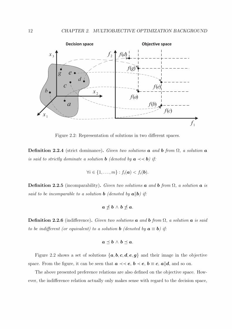
Figure 2.2: Representation of solutions in two different spaces.
Definition 2.2.4 (strict dominance). Given two solutions a and b from Ω, a solution a
is said to strictly dominate a solution b (denoted by a ≺≺ b) if:
∀i ∈ 1, . . . ,m : fi(a) < fi(b).
Definition 2.2.5 (incomparability). Given two solutions a and b from Ω, a solution a is
said to be incomparable to a solution b (denoted by a‖b) if:
a b ∧ b a.
Definition 2.2.6 (indifference). Given two solutions a and b from Ω, a solution a is said
to be indifferent (or equivalent) to a solution b (denoted by a ≡ b) if:
a b ∧ b a.
Figure 2.2 shows a set of solutions a, b, c,d, e, g and their image in the objective
space. From the figure, it can be seen that a ≺≺ e, b ≺ e, b ≡ c, a‖d, and so on.
The above presented preference relations are also defined on the objective space. How-
ever, the indifference relation actually only makes sense with regard to the decision space,

2.2. GENERAL CONCEPTS 13
1f
2f
2x
3x
1x
Decision space Objective space
a)(af
b
)(bf
)(af
Figure 2.3: Representation of the additive ε-dominance.
as in the objective space, it simply means equality. In addition, another widely used pref-
erence relation, called ε-dominance, is defined. Under ε-dominance, the conditions required
for one solution to dominate another are relaxed.
Definition 2.2.7 (multiplicative ε-dominance). Given two solutions a and b from Ω, a
solution a is said to ε-dominate a solution b (denoted by a ε b) if for a given ε:
∀i ∈ 1, . . . ,m : (1− ε)fi(a) ≤ fi(b).
Definition 2.2.8 (additive ε-dominance). Given two solutions a and b from Ω, a solution
a is said to ε-dominate a solution b (denoted by a ε b) if for a given ε:
∀i ∈ 1, . . . ,m : fi(a)− ε ≤ fi(b).
An illustration of the additive ε-dominance in the biobjective case is shown in Figure 2.3.
As we can see, solution a and solution b are incomparable (a‖b). The region that is
ε-dominated by solution a is composed of the area that would normally be dominated by
a plus the areas that would otherwise be nondominated with respect to a or would in fact

14 CHAPTER 2. MULTIOBJECTIVE OPTIMIZATION BACKGROUND
1f
2f
2x
3x
1x
Decision space Objective space
*x)( xf
Pareto optimal front
Figure 2.4: Representation of the Pareto optimal front.
dominate a. Thus, solution b that is nondominated with respect to a is also ε-dominated
by a (a ε b).
The concepts of optimality for multiobjective optimization are defined as follows.
Definition 2.2.9 (Pareto optimality). A solution x∗ ∈ Ω is Pareto optimal if and only if:
@y ∈ Ω : y ≺ x∗.
Definition 2.2.10 (Pareto optimal set). For a given multiobjective optimization problem
f(x), the Pareto optimal set (or Pareto set for short) is defined as:
PS∗ = x∗ ∈ Ω |@y ∈ Ω : y ≺ x∗.
Definition 2.2.11 (Pareto optimal front). For a given multiobjective optimization problem
f(x) and Pareto optimal set PS∗, the Pareto optimal front, or Pareto front (PF) for short,
is defined as:
PF∗ = f(x∗) ∈ Rm |x∗ ∈ PS∗.
Figure 2.4 illustrates the representation of the Pareto optimal front and the Pareto
optimal solution x∗.
2.2. GENERAL CONCEPTS 15
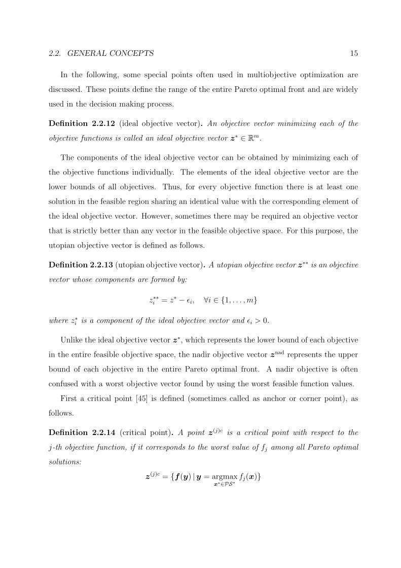
In the following, some special points often used in multiobjective optimization are
discussed. These points define the range of the entire Pareto optimal front and are widely
used in the decision making process.
Definition 2.2.12 (ideal objective vector). An objective vector minimizing each of the
objective functions is called an ideal objective vector z∗ ∈ Rm.
The components of the ideal objective vector can be obtained by minimizing each of
the objective functions individually. The elements of the ideal objective vector are the
lower bounds of all objectives. Thus, for every objective function there is at least one
solution in the feasible region sharing an identical value with the corresponding element of
the ideal objective vector. However, sometimes there may be required an objective vector
that is strictly better than any vector in the feasible objective space. For this purpose, the
utopian objective vector is defined as follows.
Definition 2.2.13 (utopian objective vector). A utopian objective vector z∗∗ is an objective
vector whose components are formed by:
z∗∗i = z∗ − εi, ∀i ∈ 1, . . . ,m
where z∗i is a component of the ideal objective vector and εi > 0.
Unlike the ideal objective vector z∗, which represents the lower bound of each objective
in the entire feasible objective space, the nadir objective vector znad represents the upper
bound of each objective in the entire Pareto optimal front. A nadir objective is often
confused with a worst objective vector found by using the worst feasible function values.
First a critical point [45] is defined (sometimes called as anchor or corner point), as
follows.
Definition 2.2.14 (critical point). A point z(j)c is a critical point with respect to the
j-th objective function, if it corresponds to the worst value of fj among all Pareto optimal
solutions:
z(j)c = f(y) |y = argmaxx∗∈PS∗
fj(x)

16 CHAPTER 2. MULTIOBJECTIVE OPTIMIZATION BACKGROUND
1f
2f worstz
cz )1(
cz )2(
z
nadz
z
Objective space
Feasible objective
region
Pareto optimal
front
Figure 2.5: Representation of some special points in multiobjective optimization.
The nadir objective vector can be defined as follows.
Definition 2.2.15 (nadir objective vector). An objective vector whose j-th element is
taken from the j-th component of the corresponding critical Pareto point is called a nadir
objective vector znad = (znad1 , . . . , znad
m )T where (znadj = z
(j)cj ).
Figure 2.5 illustrates the ideal objective vector z∗, the nadir objective vector znad, the
critical points z(1,2)c, and the worst objective vector zworst.
The ideal and nadir objective vectors represent the lower and upper bound of the Pareto
front for a given multiobjective optimization problem. The reliable estimation of both these
vectors is an important issue in multiobjective optimization. However, the estimation of
the nadir objective vector may be a quite difficult task. Usually, this involves computing
individual optimal solutions for objectives, constructing a payoff table by evaluating other
objective values at these optimal solutions, and estimating the nadir point from the worst
objective values from the table. This procedure may not guarantee a true estimation of
the nadir point for more than two objectives. Thus, in the majority of cases an estimation
of the nadir objective vector requires information about the whole Pareto optimal front.
The ideal objective vector and the nadir objective vector are used to normalize objec-

2.3. OPTIMALITY CONDITIONS 17
tive functions thereby mapping their values onto the interval [0, 1]. The normalization is
performed as follows:
f i =fi − z∗iznadi − z∗i
, ∀i ∈ 1, . . . ,m,
where f i is the normalized objective value.
2.3 Optimality Conditions
Optimality conditions are an important issue in optimization. Therefore, this section
presents a set of theoretical optimality conditions for a multiobjective optimization prob-
lem. As in single-objective optimization, there are first- and second-order optimality con-
ditions for multiobjective optimization. In the following, a multiobjective optimization
problem under consideration is of the form:
minimize: f(x) = (f1(x), f2(x), . . . , fm(x))T
subject to: x ∈ Ω,(2.3.1)
where Ω = x ∈ Rn | g(x) = (g1(x), g2(x), . . . , gp(x))T ≤ 0.
Furthermore, the set of active constraints at a point x∗ is denoted by:
J(x∗) = j ∈ 1, . . . , p | gj(x∗) = 0.
All optimality conditions provided in this section assume that all objectives and con-
straint functions are continuously differentiable. Thus, the following definitions need to be
established first.
Definition 2.3.1 (nondifferentiable MOP). The multiobjective optimization problem is
nondifferentiable if some of the objectives or the constraints forming the feasible region are
nondifferentiable.
Definition 2.3.2 (continuous MOP). If the feasible region Ω is a closed and connected
region in Rn and all the objectives are continuous of x then the multiobjective optimization
problem is called continuous.

18 CHAPTER 2. MULTIOBJECTIVE OPTIMIZATION BACKGROUND
Before a convex multiobjective problem is discussed, the definition of a convex function
is presented.
Definition 2.3.3 (convex function). A function f : Rn → R is a convex function if for
any two pairs of solutions x,y ∈ Rn, the following condition is true:
f(αx+ (1− α)y) ≤ αf(x) + (1− α)f(y),
for all 0 ≤ α ≤ 1.
Definition 2.3.4 (convex MOP). The multiobjective optimization problem is convex if all
objective functions and the feasible region are convex.
The convexity is an important matter to multiobjective optimization algorithms. Sim-
ilarly to the property of a convex function, the following theorem establishes a relation
between a local and a global Pareto optimal solution for a multiobjective optimization
problem.
Theorem 2.3.1. Let the multiobjective optimization problem be convex. Then every
locally Pareto optimal solution is also globally Pareto optimal solution.
For a proof, see Miettinen [133].
2.3.1 First-Order Conditions
The following condition is known as the necessary condition for Pareto optimality.
Theorem 2.3.2 (Fritz-John necessary condition for Pareto optimality). Let the objective
and the constraint functions of the problem shown in (2.3.1) be continuously differentiable
at a decision vector x∗ ∈ Ω. A necessary condition for x∗ to be Pareto optimal is that
there exist vectors λ ≥ 0 and µ ≥ 0 (where λ ∈ Rm, µ ∈ Rp and λ,µ 6= 0) such that:
1.m∑i=1
λi∇fi(x∗) +p∑j=1
µj∇gj(x∗) = 0
2. µjgj(x∗) = 0, ∀j ∈ 1, . . . , p.

2.3. OPTIMALITY CONDITIONS 19
For a proof, see Da Cunha and Polak [38].
If the multiobjective optimization problem is convex, then there can be stated a suffi-
cient condition for Pareto optimality. Thus, the following theorem offers sufficient condi-
tions for a solution to be Pareto optimal for convex functions.
Theorem 2.3.3 (Karush-Kuhn-Tucker sufficient condition for Pareto optimality). Let
the objective and the constraint functions of problem shown in (2.3.1) be convex and
continuously differentiable at a decision vector x∗ ∈ Ω. A sufficient condition for x∗ to be
Pareto optimal is that there exist vectors λ > 0 and µ ≥ 0 (where λ ∈ Rm, µ ∈ Rp) such
that:
1.m∑i=1
λi∇fi(x∗) +p∑j=1
µj∇gj(x∗) = 0
2. µjgj(x∗) = 0, ∀j ∈ 1, . . . , p.
For a proof, see Miettinen [133].
2.3.2 Second-Order Conditions
Second-order optimality conditions reduce the set of candidate solutions produced by the
first-order conditions. However, they tighten the assumptions set to the regularity of the
problem.
Furthermore, a definition of the regularity of decision vector follows.
Definition 2.3.5. A point x∗ ∈ Ω is said to be a regular point if the gradients of the active
constraints at x∗ are linearly independent.
The following theorem provides second-order necessary optimality conditions.
Theorem 2.3.4 (second-order necessary condition for Pareto optimality). Let the objec-
tive and the constraint functions of the problem shown in (2.3.1) be twice continuously
differentiable at a regular decision vector x∗ ∈ Ω. A necessary condition for x∗ to be
Pareto optimal is that there exist vectors λ ≥ 0 and µ ≥ 0 (where λ ∈ Rm, µ ∈ Rp and
λ 6= 0) such that:
20 CHAPTER 2. MULTIOBJECTIVE OPTIMIZATION BACKGROUND
1.m∑i=1
λi∇fi(x∗) +p∑j=1
µj∇gj(x∗) = 0
2. µjgj(x∗) = 0, ∀j ∈ 1, . . . , p
3. dT
(m∑i=1
λi∇2fi(x∗) +
p∑j=1
µj∇2gj(x∗)
)d ≥ 0,
∀d ∈ d ∈ Rn |d 6= 0, ∀i ∈ 1, . . . ,m : ∇fi(x∗)Td ≤ 0, ∀j ∈ J(x∗) : ∇gj(x∗)Td = 0.
For a proof, see Wang [185].
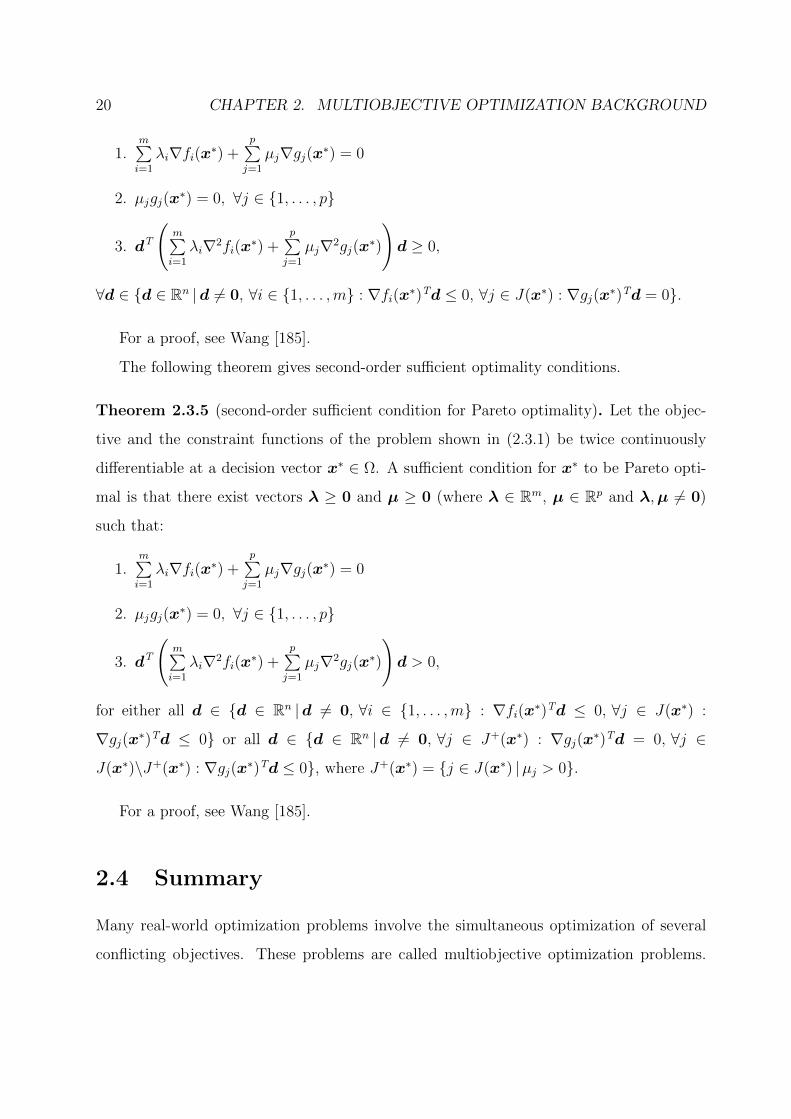
The following theorem gives second-order sufficient optimality conditions.
Theorem 2.3.5 (second-order sufficient condition for Pareto optimality). Let the objec-
tive and the constraint functions of the problem shown in (2.3.1) be twice continuously
differentiable at a decision vector x∗ ∈ Ω. A sufficient condition for x∗ to be Pareto opti-
mal is that there exist vectors λ ≥ 0 and µ ≥ 0 (where λ ∈ Rm, µ ∈ Rp and λ,µ 6= 0)
such that:
1.m∑i=1
λi∇fi(x∗) +p∑j=1
µj∇gj(x∗) = 0
2. µjgj(x∗) = 0, ∀j ∈ 1, . . . , p
3. dT
(m∑i=1
λi∇2fi(x∗) +
p∑j=1
µj∇2gj(x∗)
)d > 0,
for either all d ∈ d ∈ Rn |d 6= 0, ∀i ∈ 1, . . . ,m : ∇fi(x∗)Td ≤ 0, ∀j ∈ J(x∗) :
∇gj(x∗)Td ≤ 0 or all d ∈ d ∈ Rn |d 6= 0, ∀j ∈ J+(x∗) : ∇gj(x∗)Td = 0, ∀j ∈
J(x∗)\J+(x∗) : ∇gj(x∗)Td ≤ 0, where J+(x∗) = j ∈ J(x∗) |µj > 0.
For a proof, see Wang [185].
2.4 Summary
Many real-world optimization problems involve the simultaneous optimization of several
conflicting objectives. These problems are called multiobjective optimization problems.

2.4. SUMMARY 21
Since the objectives are in conflict, there is no single solution to the problems, but a
set of compromise solutions representing the different trade-offs with respect to the given
objective functions. This set is generally known as the set of Pareto optimal solutions.
The main goal in multiobjective optimization is to find a set of solutions that ap-
proximates the set of Pareto optimal solutions as well as possible. Since without further
preference information none of these solutions can be said superior than other, it is impor-
tant to find as many Pareto optimal solutions as possible. Therefore, there are two goals
in multiobjective optimization: (i) to find a set of solutions as close as possible to the true
Pareto optimal front, and (ii) to find a set of solutions as diverse as possible.
The first goal is identical to the goal of convergence in single-objective optimization.
However, the second goal is specific to multiobjective optimization. Additionally, all well-
distributed Pareto optimal solutions should cover the entire Pareto optimal region. A
diverse set of solutions assures a good set of trade-off solutions. The concept of diversity
can be defined either in the decision space or in the objective space. However, the diversity
in one space does not guarantee the diversity in the other space.
Since both goals are important, a multiobjective optimization algorithm must satisfy
both of them. When designing an efficient multiobjective algorithm, it should be realized
that the achievement of one goal does not necessarily achieve the other goal. Therefore,
explicit or implicit mechanisms of ensuring the convergence to the Pareto optimal region as
well as the maintenance of a diverse set of solutions must be implemented in an algorithm.
Due to these dual tasks, multiobjective optimization is more difficult than single-objective
optimization.

22 CHAPTER 2. MULTIOBJECTIVE OPTIMIZATION BACKGROUND

Chapter 3
Multiobjective Optimization
Algorithms
3.1 Introduction
The previous chapter presents the essential background necessary for dealing with multiob-
jective optimization. The present chapter discusses some of the most prominent approaches
developed for solving multiobjective optimization problems. In general, there is a large va-
riety of such methods, and all of these methods can be classified in according to different
criteria.
A general and probably most commonly used way for categorizing the methods is
by differentiating into the so-called classical methods and evolutionary algorithms. Such
classification is mainly based on the working principles for finding Pareto optimal solutions.
Additionally, according to the participation of the decision maker in the solution process,
all methods can be classified as [133]:
• No-preference methods (no articulation of preference information is used),
• A posteriori methods (a posteriori articulation of preference information is used),
• A priori methods (a priori articulation of preference information is used),
23

24 CHAPTER 3. MULTIOBJECTIVE OPTIMIZATION ALGORITHMS
• Interactive methods (progressive articulation of preference information is used).
As the name suggests, no-preference methods do not use any preference information
and do not rely on any assumptions about the importance of objectives. These methods
do not make an attempt to find multiple Pareto optimal solutions. Instead, the distance
between some reference point and the feasible objective region is minimized to find a single
optimal solution. A posteriori methods aim at finding multiple Pareto optimal solutions.
After the Pareto optimal set has been generated, it is presented to the decision maker, who
selects the most preferred solution among the alternatives. In the case of a priori methods,
the decision maker specifies his preferences before the search process. Then one preferred
solution or a subset of Pareto optimal solutions that satisfies these preferences is found
and presented to the decision maker. In interactive methods the preference information
is used progressively during the search process. The decision maker works together with
a computer program to answer some questions or provide additional information after a
certain number of iterations. The focus of the present thesis is on a posteriori methods.
Multiobjective evolutionary algorithms became very popular due to their ability to
simultaneously deal with a set of solutions and to approximate the Pareto set in a sin-
gle run. They can be also classified in various ways. For example, in the first book on
evolutionary multiobjective optimization [42] they are classified into non-elitist and elitist
approaches. On the other hand, MOEAs can be differentiated according to the princi-
ples of performing the search either in the decision or objective space. Concerning the
objective space, the selection of promising solutions is made based on the fitness assigned
to the population members. Therefore, one can categorize MOEAs according to the fit-
ness assignment mechanisms as: dominance-based, scalarizing-based, and indicator-based.
Dominance-based approaches calculate an individual’s fitness on the basis of the Pareto
dominance. Scalarizing-based approaches use traditional mathematical techniques based
on the aggregation of multiple objectives into a single parameterized objective to assign
a scalar fitness value to each individual in the population. In turn, indicator-based ap-
proaches, which are a relatively recent trend in EMO, employ performance indicators to

3.2. CLASSICAL METHODS 25
assign fitness to individuals in the current population.
Another way to classify MOEAs is based on how the search is performed in the deci-
sion space. In other words, the classification is based on how new candidate solutions are
generated (i.e., based on the variation operators of EAs). This classification is adopted in
this thesis to discuss different state-of-the-art MOEAs, except for MOEAs based on de-
composition that are put in a distinct category. Furthermore, due to the growing attention
to the field of many-objective optimization, evolutionary algorithms designed specifically
to deal with many-objective problems are discussed separately. The fitness assignment
and selection process are the main features under consideration in these algorithms. As a
final remark, it should be noted that the herein presented classifications are not absolute,
overlapping and combinations of different categories are possible. Some methods can be
put in more than one category. All classifications are for guidance only.
3.2 Classical Methods
Classical methods have been studied in literature for nearly last six decades. Each of
them has its own strengths and weaknesses. However, the proofs of convergence to the
Pareto optimal set are their main strength. In the following, a few classical methods for
multiobjective optimization are discussed.
3.2.1 Weighted Sum Method
The weighted sum method [75] associates each objective function with a weighting coeffi-
cient and minimizes the weighted sum of the objectives. In this way, the multiple objective
functions are transformed into a single objective function. Thus, the original MOP results
26 CHAPTER 3. MULTIOBJECTIVE OPTIMIZATION ALGORITHMS
01f
2f
2/wy
21/ww
21/ww
A
B
C
D
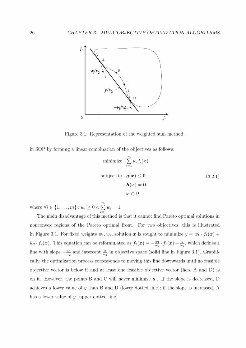
Figure 3.1: Representation of the weighted sum method.
in SOP by forming a linear combination of the objectives as follows:
minimizem∑i=1
wifi(x)
subject to g(x) ≤ 0
h(x) = 0
x ∈ Ω
(3.2.1)
where ∀i ∈ 1, . . . ,m : wi ≥ 0 ∧m∑i=1
wi = 1.
The main disadvantage of this method is that it cannot find Pareto optimal solutions in
nonconvex regions of the Pareto optimal front. For two objectives, this is illustrated
in Figure 3.1. For fixed weights w1, w2, solution x is sought to minimize y = w1 · f1(x) +
w2 · f2(x). This equation can be reformulated as f2(x) = −w1
w2· f1(x) + y
w2, which defines a
line with slope −w1
w2and intercept y
w2in objective space (solid line in Figure 3.1). Graphi-
cally, the optimization process corresponds to moving this line downwards until no feasible
objective vector is below it and at least one feasible objective vector (here A and D) is
on it. However, the points B and C will never minimize y . If the slope is decreased, D
achieves a lower value of y than B and D (lower dotted line); if the slope is increased, A
has a lower value of y (upper dotted line).

3.2. CLASSICAL METHODS 27
01f
2f
A
B
C
D
2
feasible
infeasible
2'
Figure 3.2: Representation of the ε-constraint method.
3.2.2 ε-Constraint Method
In the ε-constraint method, introduced in Haimes et al. [78], one of the objective functions is
selected to be optimized and all the other objective functions are converted into constraints
by setting an upper bound to each of them. The problem to be solved is now of the form:
minimize fl(x)
subject to fi(x) ≤ εi, ∀i ∈ 1, . . . ,m ∧ i 6= l
g(x) ≤ 0
h(x) = 0
x ∈ Ω
(3.2.2)
In the above formulation, the parameter εi represents an upper bound of the value of fi.
The working principle of the ε-constraint method for two objectives is shown in Figure 3.2.
The function f1(x) is retained and optimized whereas f2(x) is treated as a constraint:
f2(x) ≤ ε2. The optimal solution of this problem is the point C. It can be easily seen
that the method is able to obtain solutions in convex as well as nonconvex regions of the
Pareto optimal front. However, if the upper bounds are not chosen appropriately (ε′2), the
obtained new feasible set might be empty, i.e., there is no solution to the corresponding

28 CHAPTER 3. MULTIOBJECTIVE OPTIMIZATION ALGORITHMS
SOP. In order to avoid this situation, a suitable range of values for the εi has to been
known beforehand.
3.2.3 Weighted Metric Methods
In the weighted metric methods, the distance between some reference point and the feasible
objective region is minimized. For this purpose, the weighted Lp metrics are used for
measuring the distance of any solution from the reference point. The ideal objective vector
is often used as the reference point. Thus, the weighted Lp-problem is of the form:
minimize
(m∑i=1
wi|fi(x)− z∗i |p)1/p
subject to g(x) ≤ 0
h(x) = 0
x ∈ Ω
(3.2.3)
The parameter p can take any value between and 1 and ∞. When p = 1 is used,
the resulting problem is equivalent to the weighted sum approach (if z∗ = 0). When
p = 2 is used, a weighted Euclidean distance of any point in the objective space from the
ideal point is minimized. When p gets larger, the minimization of the largest deviation
becomes more and more important. When p = ∞, the only thing that matters is the
weighted relative deviation of one objective function, and the above problem reduces to
the following problem:
minimize: max1≤i≤m
wi|fi(x)− z∗i |
subject to: g(x) ≤ 0
h(x) = 0
x ∈ Ω
(3.2.4)
Problem shown in (3.2.4) was originally introduced in Bowman [106], and it is called
the weighted Chebyshev problem. In literature, the name of the above problem may vary
due to the different ways of spelling.

3.2. CLASSICAL METHODS 29
01f
2fA
B
C
DZ*
(a) The weighted metric method with p = 1
0
1f
2fA
B
C
DZ*
(b) The weighted metric method with p = 2
0
1f
2f
A
B
Z*
(c) The weighted metric method with p =∞
Figure 3.3: Representation of the weighted metric method.

30 CHAPTER 3. MULTIOBJECTIVE OPTIMIZATION ALGORITHMS
However, the resulting optimal solution obtained by the chosen Lp depends on the
parameter p. The working principle of this method for two objectives is illustrated in
Figures 3.3(a), 3.3(b) and 3.3(c) for p = 1, 2 and ∞, respectively.
In all these figures, optimal solutions for two different weight vectors are shown. It is
clear that with p = 1 or 2, not all Pareto optimal solutions can be obtained. In these
cases, the figures show that no solution in the region BC can be found by using p = 1 or 2.
However, when the weighted Chebyshev metric is used (Figure 3.3(c)), any Pareto optimal
solution can be found. The theorem which states that every Pareto optimal solution can be
obtained by the weighted Chebyshev method and its prove can be found in Miettinen [133].
It is important to note that even differentiable multiobjective problem becomes nondif-
ferentiable using the weighted Chebyshev method. On the other hand, for the low values
of p if the original MOP is differentiable the resulting SOP remains also differentiable and
it can be solved using gradient-based methods. Another difficulty may arise from dealing
with the objectives of different orders of magnitude. In this case, it is advisable to normal-
ize the objective functions. In turn, this requires a knowledge of minimum and maximum
function values of each objective. Moreover, this method also requires the ideal solution
z∗. Therefore, all m objectives need to be independently optimized before optimizing the
Lp metric.
3.2.4 Normal Boundary Intersection Method
Das and Denis [39] proposed the normal boundary intersection (NBI) method, which at-
tempts to find multiple Pareto optimal solutions of a given multiobjective problem by
converting it into a number of single objective constrained problems. In the NBI method,
it is assumed that the vector of global minima of the objectives (f ∗) is available. The
convex hull is obtained using the individual minimum of the functions. Then, the simplex
is constructed by the convex hull of the individual minimum and is expressed as Φβ. The
NBI scalarization scheme takes a point on the simplex and then searches for the maximum
distance along the normal pointing toward the origin. This obtained point may or may

3.2. CLASSICAL METHODS 31
01f
2f
A
aB
bC
cD
d E
e
F
f
G
g
H
h
I
iJKLMj
klm
1f
2f
Figure 3.4: Representation of the normal boundary intersection method.
not be a Pareto optimal point. The NBI subproblem for a given vector β is of the form:
maximize : t
subject to Φβ + tn = f(x)
g(x) ≤ 0
h(x) = 0
x ∈ Ω
(3.2.5)
where ∀i ∈ 1, . . . ,m : βi ≥ 0 ∧m∑i=1
βi = 1, Φ = [f(x1∗),f(x2∗), . . . ,f(xm∗)] is a m ×m
matrix, xi∗ is the minimizer of the i-th individual objective function (xi∗ = arg minxfi(x)),
n is the normal direction at the point Φβ pointing towards the origin. The solution of
the above problem gives the maximum t and also the corresponding approximation to the
Pareto optimal solution x. The method works even when the normal direction is not an
exact one, but a quasi-normal direction. The following quasi-normal direction vector is
suggested in Das and Denis [39]: n = −Φe, where e = (1, 1, . . . , 1)T is a m × 1 vector.
The above quasi-normal direction has the property that NBIβ is independent of the relative
scales of the objective functions.
Figure 3.4 illustrates the working principle of the NBI method. It shows the solutions
a, b, c, d, e, f, g, h, i, j, k, l,m obtained from the points A,B,C,D,E, F,G,H, I, J,K, L,M

32 CHAPTER 3. MULTIOBJECTIVE OPTIMIZATION ALGORITHMS
0
1f 2f
3f)( *3xf
Inaccessibleregions
)( *1xf )( *2xf
Figure 3.5: Pareto optimal solutions not obtainable using the NBI method.
on the convex hull (Φ = [f 1∗ f 2∗]) by solving the NBI subproblems for the different vectors
β. The method can find solutions in convex and nonconvex regions of the Pareto front. It
can be seen that points f, g, h are not Pareto optimal but are still found using the NBI
method.
Besides sometimes non-Pareto optimal solutions are obtained, another limitation of the
NBI method is that for dimensions more than two, the extreme Pareto optimal solutions
are not obtainable in all the cases. This limitation is due to the restriction of 0 ≤ β ≤ 1
parameters. This can be easily seen by considering a problem having a spherical Pareto
front satisfying f 21 + f 2
2 + f 23 in the range ∀i ∈ 1, . . . ,m: 0 ≤ fi ≤ 1. As seen from
Figure 3.5, there are unexplored regions outside the simplex obtained by the convex hull
of individual function minima.
3.2.5 Normal Constraint Method
Messac and Mattson [130] proposed the normal constraint (NC) method for generating
a set of evenly spaced Pareto optimal solutions. To describe the NC method, the fol-
lowing notations are introduced first. The NC method uses the normalized function
values to cope with disparate function scales. The normalized objective vectors (f =
3.2. CLASSICAL METHODS 33
(f 1, . . . , fm)T) are computed using the ideal (f ideal = (f ideal1 , . . . , f ideal
m )T) and the nadir
(fnadir = (fnadir1 , . . . , fnadir
m )T) objective vectors. The following equation is used to perform
the mapping:
f i =fi − f ideal
i
fnadiri − f ideal
i
, ∀i ∈ 1, . . . ,m.
The points µi∗ = f(xi∗) ∀i ∈ 1, . . . ,m are called the anchor points, where xi∗ is
the minimizer of the i-th objective. The normalized anchor points are denoted as µi∗
∀i ∈ 1, . . . ,m. The m-dimensional hyperplane passing through the anchor points is
constructed. A set of evenly distributed point is generated on the hyperplane. Any point
on the hyperplane can be defined as a function of the anchor points:
z = Φβ
where z is a point on the hyperplane corresponding to a given vector β which satisfies
∀i ∈ 1, . . . ,m : 0 ≤ βi ≤ 1 ∧m∑i=1
βi = 1,
and Φ = (µ1∗, . . . ,µm∗] is a m×m matrix.
The vectors to fixed anchor point µl∗ from other anchor points are computed:
vi = µl∗ − µi∗, ∀i ∈ 1, . . . ,m ∧ i 6= l.
Finally, the NC subproblem for a given point z on the constructed hyperplane is of the
form:
minimize f l(x)
subject to vTi (f(x)− z) ≤ 0, ∀i ∈ 1, . . . ,m ∧ i 6= l
g(x) ≤ 0
h(x) = 0
x ∈ Ω
(3.2.6)
The normal constraint method uses an inequality constraint reduction of the feasible
space. Figure 3.6 shows the obtained solution using the NC method for two objectives.
The hatched part is the feasible region corresponding to point B in the ideal plane. It can

34 CHAPTER 3. MULTIOBJECTIVE OPTIMIZATION ALGORITHMS
01f
2fReduced Feasible
Region
1
2
B
b
Figure 3.6: Representation of the NC method.
be seen that point b is not Pareto optimal but it is still found using the NC method. Since
evenly distributed points on the ideal plane are used, the final points on the Pareto front
are likely to be more evenly distributed than using the usual ε-constraint method.
3.2.6 Timmel’s Method
Timmel [174] proposed a stochastic approach for finding multiple Pareto optimal solutions
of a differentiable multiobjective optimization problem. It is a population based approach,
where for a given parent solution, a child solution is created in the following manner:
xchild = xparent − tkm∑i=1
ui∇fi(xparent) (3.2.7)
where xparent is the parent decision vector, xchild is the generated child decision vector,
∇fi(xparent) is the gradient of the i-th objective function, tk is the step size at the k-th
iteration and ui is a uniformly distributed random number between zero and one
(ui ∼ U(0, 1)).
The above formulation ensures that not all objective functions can be worsened simul-
taneously. Thus, the child solution xchild is either nondominated when compared to the

3.2. CLASSICAL METHODS 35
01f
2fA
B
C
D
a
b
c
d
Figure 3.7: Representation of Timmel’s method.
parent solution xparent, or it dominates the parent solution. The variation of the step size t
over iterations must be made carefully to ensure convergence to the Pareto optimal front.
In general, the step size update scheme must ensure the following aspects: (i) the step size
should slowly decrease to zero as solutions closer to the Pareto optimal set are found; (ii)
the decrease of the step size must not be slow enough so that the algorithm gets caught in
suboptimal regions.
Figure 3.7 shows the creation of child solutions a, b, c, d (denoted by the lowercase
letters) from the corresponding parents (denoted by the capital letters). The vectors of
the gradients are presented for the parent solution C. The child solution c is generated
by adding the linear combination of the gradients to the parent solution C. For the other
parent solutions children are generated in the same way. It can be seen that not all children
dominate their parents. After the child population is created, it is combined with the
parent population and only nondominated solutions are retained. Then, this set becomes
the parent population, and this procedure is repeated for a specified number of iterations.
The population size can vary with iterations, if fact, an increase in the population size is
expected in most of the problems. It is interesting to note that this algorithm uses an
elitist strategy, in which the best individuals from parents and offspring are retained.

36 CHAPTER 3. MULTIOBJECTIVE OPTIMIZATION ALGORITHMS
3.3 Evolutionary Multiobjective Optimization
Algorithms
The term evolutionary algorithm stands for a class of stochastic optimization methods that
simulate the process of natural evolution [199]. The origins of EAs can be traced back to
the late 1950s, however, the field remained relatively unknown to the broader scientific
community for almost three decades. This was largely due to the lack of available powerful
computer platforms at that time, but also due to some methodological shortcomings of
those early approaches. Since the 1970s several evolutionary methodologies have been pro-
posed, mainly genetic algorithms, evolutionary programming, and evolution strategies [4].
Evolutionary algorithms are particularly suitable for solving multiobjective optimiza-
tion problems because they deal simultaneously with a set of possible solutions, called
population, which allows to find several Pareto optimal solutions in a single run of the
algorithm, instead of having to perform multiple runs with different parameter settings as
in the case of the majority of classical methods for multiobjective optimization.
In the following, a number of state-of-the-art EMO algorithms are discussed. All al-
gorithms are structured according to variation operators, except for MOEAs based on
decomposition, which are put in a distinct category. A number of other approaches, such
as indicator-based and scalarizing-based algorithms as well as algorithms designed specifi-
cally to handle many-objective optimization problems are discussed in the next section.
3.3.1 Genetic Algorithm-Based Approaches
The concept of a genetic algorithm (GA) was first introduced by Holland in the early 1970s
at the University of Michigan. As the name suggests, genetic algorithm is a probabilistic
search algorithm which borrows its working principal from natural selection and natural
genetics. A comprehensive description of GAs can be found in [77, 85, 132, 134].
The first actual implementation of a multiobjective evolutionary algorithm was sug-
gested by Schaffer [156]. The proposed vector evaluation genetic algorithm (VEGA) ba-

3.3. EVOLUTIONARY MULTIOBJECTIVE OPTIMIZATION ALGORITHMS 37
sically consisted of a simple genetic algorithm with a modified selection mechanism. The
population at any generation is divided into N/m subpopulations, where m is the number
of objectives and N is the population size. To each individual in each subpopulation is
assigned a fitness based on the corresponding particular objective function only. In order
to reduce the positional bias in the population, the population is shuffled before it is par-
titioned into subpopulations. After each solution is assigned a fitness, the proportionate
selection operator [77] is applied until the complete subpopulation is filled. The described
selection procedure emphasizes solutions which are good for individual objective functions.
In order to find intermediate trade-off solutions, crossover is allowed between any two so-
lutions in the entire population. In this way, the main idea is that a crossover between two
good solutions, each corresponding to a different objective, may find offspring which are
good compromised solutions between the two objectives.
The idea of calculating the fitness for individuals in the population based on the concept
of Pareto optimality was for the first time suggested by Goldberg [77]. In turn, Fonseca
and Fleming [70, 72] first proposed a multiobjective genetic algorithm (MOGA) which
explicitly emphasizes nondominated solutions and simultaneously maintains diversity in
the nondominated solutions. The proposed approach differs from a standard GA in the
way fitness is assigned to each solution in the population. The rest of the algorithm (the
stochastic universal selection, a single point crossover, and a bit-wise mutation) is the
same as that in a classical GA. First, each solution is checked for its domination in the
population. To a solution i, a rank equal to one plus the number of solutions ni that
dominate solution i is assigned: ri = 1 + ni. In this way, nondominated solutions are
assigned a rank equal to 1, since no solution would dominate a nondominated solution in
a population. Therefore, there must be at least one solution with rank equal to one and
the maximum rank of any population member cannot be more than N (the population
size). In order to maintain diversity among nondominated solutions, the authors have
introduced niching among solutions of each rank. A shared fitness value is calculated by
dividing the fitness of a solution by its niche count. In order to keep the average fitness
of the solutions in a rank the same as that before sharing, these fitness values are scaled

38 CHAPTER 3. MULTIOBJECTIVE OPTIMIZATION ALGORITHMS
so that their average shared fitness value is the same as the average assigned fitness value.
After these calculations, the focus is shifted to the solutions of the next rank and an
identical procedure is executed. This procedure is continued until all ranks are processed.
Thereafter, the stochastic universal selection based on shared fitness values, the single point
crossover, and the bit-wise mutation operators are applied to create a new population.
Goldberg’s idea of using the nondominated sorting concept in GAs was more directly
implemented by Srinivas and Deb [164]. The proposed approach, called nondominated
sorting genetic algorithm (NSGA), uses a fitness assignment scheme which prefers nondom-
inated solutions and employs a sharing strategy which preserves diversity among solutions
of each nondominated front. The first step in NSGA is to sort the population P according
to non-domination. The fitness assignment procedure begins from the first nondominated
set and successively proceeds to dominated sets. Any solution i of the first nondominated
set is assigned a fitness equal to Fi = N (the population size). In this way, assigning more
fitness to solutions belonging to a better nondominated set ensures a selection pressure
towards the Pareto optimal front. In order to promote the diversity among solutions the
sharing function method is used which degrades the assigned fitness based on the num-
ber of neighboring solutions. That is, for each solution i in the front Pj, the normalized
Euclidean distance dij (in the decision space) from another solution j in the same front
is calculated. Once these distances are calculated, they are used to compute a sharing
function. The sharing function takes a value between zero and one, depending on the
distance dij . Any solution j which has a distance greater than σshare from the i-th solution
contributes nothing to the sharing function value. After all |Pj| sharing function values are
calculated, they are added together to calculate the niche count nci, of the i-th solution.
The niche count, in some sense, denotes the number of solutions in the neighborhood of
the i-th solution, including the latter. If there exists no other solution within a radius of
σshare from a solution the niche count for that solution would be one. On the other hand, if
|Pj| solutions in the front are very close to each other compared to σshare, the niche count
of any solution in the group would be close to |Pj|. When the niche count is calculated, the
fitness of the i-th solution is reduced as F ′i = Fi/nci. This process of degrading fitness of

3.3. EVOLUTIONARY MULTIOBJECTIVE OPTIMIZATION ALGORITHMS 39
a solution, which is crowded by many solutions, helps to emphasize the solutions residing
in less crowded regions. This procedure completes the fitness assignment procedure of all
solutions in the first front. Thereafter, a fitness value slightly smaller than the minimum
shared fitness in the first front is assigned to solutions in the second nondominated front.
This makes sure that no solution in the first front has a shared fitness worse than the as-
signed fitness of any solution in the second front. Once again, the sharing function method
is applied among the solutions of the second front and the corresponding shared fitness
values are computed. Next this procedure is applied to subsequent fronts until all solutions
in the population are assigned a shared fitness. Finally, the assigned shared fitness is used
to select the mating pool and genetic operators are applied to produce a new population.
Deb et al. [46] suggested an elitist nondominated sorting genetic algorithm (NSGA-II).
In NSGA-II, each solution in the current population P is evaluated using Pareto ranking
and a crowding measure. First the best rank is assigned to all the nondominated solutions
in the current population. Solutions with the best rank are removed from the current
population. Next, the second best rank is assigned to all the nondominated solutions in
the remaining population. In this manner, ranks are assigned to all solutions in the current
population. A fast nondominated sorting procedure was also proposed. Then, a binary
tournament selection based on non-domination rank and crowding distance is performed
to select a set of parent solutions. That is, when two solutions are selected, the one with
the lower non-domination rank is preferred. Otherwise, if both solutions belong to the
same rank, then the solution with the higher crowding distance is selected. Next, genetic
operators such as recombination and mutation are applied to create an offspring population
Q. Then, the two populations are merged together to form a combined population Rt =
Pt ∪ Qt. Next, the combined population is sorted according to different nondominated
front. If the size of the first nondominated front F1 is smaller then N , all members of
the set F1 are chosen for the new population. The remaining members of the population
Pt+1 are chosen from subsequent nondominated fronts in the order of their ranking. Thus,
solutions from the set F2 are chosen next, followed by solutions from the set F3, and so on.
This procedure is continued until no more sets can be accommodated. Say that the set Fl

40 CHAPTER 3. MULTIOBJECTIVE OPTIMIZATION ALGORITHMS
is the last nondominated set beyond which no other set can be accommodated. In general,
the count of solutions in all sets from F1 to Fl would be larger than the population size.
To choose exactly N population members, the solutions of the last nondominated front Flare sorted using the crowding distance in descending order and choose the best solutions
needed to fill all population slots. Then the algorithm proceeds to the next iteration and
the new population Pt+1 is used for selection, crossover, and mutation to create a new
population Qt+1.
Zitzler and Thiele [195, 201] proposed a strength Pareto evolutionary algorithm (SPEA).
SPEA uses a regular population and an archive to store nondominated solutions. The algo-
rithm starts by randomly creating an initial population P0 of size N and an empty archive
A0 with a maximum capacity of N . In any generation t, the nondominated solutions of
the population Pt are copied to the archive Pt, while any dominated individuals or du-
plicates (regarding the objective values) are removed from the archive during this update
procedure. If the size of the updated archive exceeds a predefined limit, further archive
members are deleted by a clustering technique. The fitness values are assigned to both
archive and population members. Each individual i in the archive is assigned a strength
value S(i), which at the same time represents its fitness value F (i). S(i) is the number of
population members j that are dominated by or equal to i, divided by the population size
plus one. The fitness F (j) of an individual j in the population is calculated by summing
the strength values S(i) of all archive members i that dominate or are equal to j, and
adding one at the end. Next, the mating selection is performed where individuals from
the union of population and archive are selected by means of binary tournaments. Here,
minimum fitness corresponds to better performance, so each individual in the archive has
a higher chance to be selected than any population member. After a pool of parents is se-
lected, recombination and mutation are applied to generate an offspring population which
replaces the old population. Thereafter, the external archive is updated.
To overcome some drawbacks encountered in SPEA, Zitzler et al. [200] suggested an
improved version of strength Pareto evolutionary algorithm, called SPEA2. The algorithm
starts by randomly generating an initial population P0 of size N and an empty archive A0 of

3.3. EVOLUTIONARY MULTIOBJECTIVE OPTIMIZATION ALGORITHMS 41
size N . Next, the fitness values are calculated for all solutions in the population and archive.
Each individual i in the archive Pt and the population Pt is assigned a strength value S(i),
representing the number of solutions it dominates. Then the raw fitness R(i) of individual
i is calculated by summing the strengths of its dominators. Next, the density D(i) is
calculated as D(i) = 1/(σki +2), where σki is the distance to the k-th nearest solution and k
is determined as the square root of the sum of the population and archive size. Thereafter,
the fitness of individual i is calculated by adding density D(i) to the raw fitness value R(i).
Mating selection procedure performs binary tournament selection with replacement on the
archive At+1 in order to fill the mating pool. Then, recombination and mutation operators
are applied to the mating pool, the resulting set of solutions forms a new population Pt+1.
During environmental selection, all nondominated individuals from archive and population
are copied to the archive of the next generation Pt+1. If the nondominated front fits exactly
into the archive the environmental selection step is completed. In the case, when the archive
is larger than the number of nondominated solutions, the remaining slots are filled with
the best N − |Pt+1| dominated individuals from the previous archive and population. In
the case, when the size of the current nondominated set exceeds N , an archive truncation
procedure is invoked which iteratively removes individuals from Pt+1 until Pt+1 = N .
At each stage, the truncation procedure chooses the individual which has the minimum
distance to another individual. If there are several individuals with minimum distance, the
tie is broken by considering the second smallest distance and so forth.
3.3.2 Evolution Strategy-Based Approaches
Evolution strategies (ESs) are a class of stochastic search methods inspired by the theory of
evolution by means of natural selection. Its roots date back to the mid 1960s when ES was
developed by three students (Bienert, Rechenberg, Schwefel) at the Technical University
in Berlin. ESs use mutation, recombination, and selection applied to a population of
individuals containing candidate solutions in order to evolve iteratively better and better
solutions. A review of ESs for single-objective optimization can be found in [14, 15, 159].

42 CHAPTER 3. MULTIOBJECTIVE OPTIMIZATION ALGORITHMS
Knowles and Corne [112, 113] suggested a Pareto-archived evolution strategy (PAES).
The algorithm is a simple (1+1)-ES extended to multiobjective optimization. At any
generation, PAES maintains the parent a and the offspring b along with an archive of the
best solutions found so far. At first, an initial random solution a is generated and added
to the archive. It is then mutated by using a normally distributed probability function
with zero-mean and with a fixed mutation strength. The produced offspring b is evaluated.
Thereafter, both parent and offspring are compared and the winner becomes the parent of
the next generation. First, the parent a and the offspring b are compared for domination.
If a dominates b, the offspring b is discarded and a new mutated solution is created from a
for further processing. On the other hand, if b dominates a, the offspring is better than the
parent. In this case, solution b is accepted as a parent of the next generation and is added
to the archive. Otherwise, when both a and b are nondominated to each other, the offspring
is compared with the current archive, which contains the set of nondominated solutions
found so far. Three cases are possible here. In the first case, the offspring is dominated by
a member of the archive. The offspring is then rejected and the parent a is mutated again
to find a new offspring for further processing. In the second case, the offspring dominates
a member of the archive. The dominated members of the archive are deleted and the
offspring is accepted without any condition. The offspring then becomes the parent of the
next generation. In the third case, the offspring is not dominated by any member of the
archive and it also does not dominate any member of the archive. In such a case, the
offspring is added to the archive only if there is a slot available in the latter. However, the
acceptance of the offspring in the achieve does not qualify it to become the parent of the
next generation. To decide who qualifies as a parent of the next generation, the density
of solutions in their neighborhood is checked. The one residing in the least crowded area
in the search space qualifies as the parent. If the archive is full, the above density-based
comparison is performed between the parent and the offspring to decide who remains in the
archive. The adaptive grid procedure based on recursively dividing up the d-dimensional
objective space is used to estimate the density of solutions in the archive. First, each
objective is divided into 2d equal divisions, where d is a user-defined depth parameter. In

3.3. EVOLUTIONARY MULTIOBJECTIVE OPTIMIZATION ALGORITHMS 43
this way, the entire search space is divided into (2d)m unique, equal-sized m-dimensional
hypercubes. The archived solutions are placed in these hypercubes according to their
locations in the objective space. Thereafter, the number of solutions in each hypercube is
counted. If the offspring resides in a less crowded hypercube than the parent, the offspring
becomes the parent of the next generation. Otherwise, the parent solution continues to
be the parent of the next generation. If the archive is already full with nondominated
solutions, the offspring cannot be included automatically. First, the hypercube with the
highest number of solutions is identified. If the offspring does not belong to that hypercube,
it is included in the archive and at random one of the solutions from the highest-count
hypercube is eliminated. Whether the offspring or the parent qualifies to be the parent of
the next generation is decided by the same parent-offspring density count.
Costa and Oliveira [34] proposed a multiobjective elitist evolution strategy (MEES). It
is an extension of the traditional single-objective ES to multiobjective optimization. MEES
maintains the main features of ESs such as real representation of the search parameters,
self-adaptation of step sizes and recombination. Moreover, an adaptive sharing scheme
was proposed together with a geometric selection to control and guide the search. At each
generation, the algorithm maintains the main population and the secondary population
(SP). The main population is used to generate (λ + θ) offspring solutions. Offspring are
created by means of recombination and mutation common to single-objective ES, the step
size for mutation is adapted with nonisotropic self-adaptation scheme. The parameter θ
is introduced in order to control the elitist level. This parameter states the maximum
number of nondominated solutions of the secondary population that are introduced in the
main population. If the number of nondominated solutions in SP is greater or equal then
θ, then θ nondominated solutions are randomly selected from SP to constitute the elite,
otherwise all nondominated solutions are selected from SP. MEES uses the (µ+λ) selection
scheme. Fitness assignment is performed in two steps. First, the population of (µ + λ)
solutions is sorted according to non-domination and ranks are assigned to each solution.
Thereafter, in order to maintain diversity a sharing scheme is applied to the fitness values
of solutions. The fitness value of each solution is multiplied by a quantity, called niche
44 CHAPTER 3. MULTIOBJECTIVE OPTIMIZATION ALGORITHMS
count, proportional to the number of solutions having a distance inferior to a parameter
σshare. This fitness assignment procedure is repeated for all nondominated fronts separately
until all solutions are assigned with fitness values. Two selection schemes were proposed
in MEES. In the first scheme, a deterministic selection is performed in the case where
the number of solutions in the first nondominated front is not greater then µ. Otherwise,
a tournament selection is performed when the number of solutions in the first front is
greater then µ. The second scheme is more complicated, and the main idea is to select
distinct quantities of solutions from each nondominated front for the next generation. The
quantities of solutions for each front are chosen in such a way that the number of solutions
selected from the first front will be greater than the number of solutions selected from the
second front and so on. In MEES, the secondary population is used to store nondominated
solutions found during the search. During the generations, new nondominated solutions
are added to SP whereas that became dominated are eliminated. To keep SP of bounded
size, a parameter d is introduced stating the minimum desirable distance in objective space
between solutions in SP.
3.3.3 Differential Evolution-Based Approaches
Differential evolution (DE), proposed by Storn and Price in 1995 [167], is a simple and
powerful population-based stochastic direct search method for real-parameter optimization.
DE uses a simple mutation operator based on differences between pairs of solutions with
the aim of finding a search direction based on the distribution of solutions in the current
population. Since its advent, DE has attracted the attention of the researchers from diverse
domains of knowledge, all over the world. This has resulted in a plenty of variants [141,
165, 166] of the basic DE algorithm and a steadily growing number of published articles. A
comprehensive review of single-objective DE-based approaches can be found in [40, 137].
Abbass et al. [1] proposed a Pareto differential evolution (PDE) algorithm. The al-
gorithm, which uses the DE/current-to-rand/1/bin variant for reproduction, works as
follows. Only nondominated solutions are retained in the population for recombination

3.3. EVOLUTIONARY MULTIOBJECTIVE OPTIMIZATION ALGORITHMS 45
(all dominated solutions are removed). Three parents are randomly selected (one as the
main parent and also trial solution) and a child is generated using these solutions. The
offspring is placed in the population only if it dominates the main parent. Otherwise, a
new selection process takes place. This process continues until the population is completed.
If the number of nondominated solutions exceeds a certain threshold, a distance metric is
adopted to remove parents, which are too close from each other. In this approach, the
scaling parameter F is generated from a Gaussian distribution N(0, 1) and the boundary
constraints are preserved either by reversing the sign if the variable is less than zero or by
repetitively subtracting one if it is greater then zero, until the variable is within the allow-
able boundaries. The algorithm also incorporates a mutation operator, which is applied
after the crossover with a certain probability, in order to add a small variation to each
variable.
Iorio and Li [96] proposed a nondominated sorting differential evolution (NSDE). This
approach is a simple modification of the NSGA-II. The only difference between this ap-
proach and NSGA-II is in the method for generating new individuals. In NSDE, simulated
binary crossover (SBX) and polynomial mutation operators are replaced by the DE opera-
tors. New candidates are generated using the DE/current-to-rand/1/bin variant, which is
known to be rotationally invariant. A number of experiments are conducted on a unimodal
rotated problem. Comparing the results produced by NSDE and NSGA-II, it was shown
that DE can provide rotationally invariant behavior on a multiobjective optimization prob-
lem.
Santana-Quintero and Coello Coello [149] proposed ε-MyDE. This approach keeps two
populations: the main population to select the parents and the secondary population,
in which the concept of ε-dominance is adopted to retain and to uniformly distribute
nondominated solutions found so far. The concept of ε-dominance does not allow two so-
lutions with a difference less than εi in the i-th objective to be nondominated with respect
to each other, thereby allowing a good spread of solutions. The algorithm incorporates
a constraint-handling mechanism that allows infeasible solutions to intervene during re-
combination. The DE/rand/1/bin variant is used for reproduction. After a user-defined
46 CHAPTER 3. MULTIOBJECTIVE OPTIMIZATION ALGORITHMS
number of generations is reached, three solutions used in the mutation operator are selected
from the secondary population in such a way that they are close among them in the objec-
tive space. If none of solutions satisfies this condition, other solution is randomly chosen
from the secondary population. To improve exploration capabilities, a uniform mutation
operator is used.
Kukkonen and Lampinen developed a generalized differential evolution (GDE). The
proposal extends DE/rand/1/bin to solve multiobjective optimization problems. The first
version [119] of this approach modifies the original DE selection operation by introducing
Pareto dominance as a selection criterion between the old population member and the trial
vector. Also, Pareto dominance in the constraint space is considered to handle constrained
problems.
To promote a better distribution of nondominated solutions, Kukkonen and
Lampinen [115] suggested a second version of their approach, called GDE2. In this version,
a crowding distance measure is used to select the best solution when the old population
vector and the trial vector are feasible and nondominated with respect to each other,
in such a way that the vector located in the less crowded region is selected to the next
generation. The authors acknowledge that GDE2 is sensitive to its initial parameters and
that the modified selection mechanism slows down the convergence.
To deal with the shortcomings of GDE2 regarding the slow convergence, Kukkonen
and Lampinen [116] proposed an improved version of their approach, called GDE3. This
version uses the nondominated sorting (as in NSGA-II), and allows the current population
to grow in order to improve the distribution of solutions and to decrease the sensitivity of
the approach to its initial parameters. In GDE3, when the old population member and
the trial vector are feasible and nondominated with respect to each other, both of them
are maintained. Hence, the population size grows. To maintain a fixed population size for
the next generation, the nondominated sorting is performed after each generation to prune
the population size.
A good review of the state-of-the-art multiobjective DE algorithms can be found
in [131].

3.3. EVOLUTIONARY MULTIOBJECTIVE OPTIMIZATION ALGORITHMS 47
3.3.4 Particle Swarm Optimization-Based Approaches
Particle swarm optimization (PSO) was originally proposed by Kennedy and Eberhart in
1995 [107]. The PSO algorithm is based on swarm intelligence techniques. The concept
of swarm intelligence was inspired by the social behavior of groups of animals such as a
flock of birds, a nest of ants, or a school of fish. More about PSO algorithms can be found
in [10, 11, 144].
Coello Coello et al. [30] proposed a particle swarm-based approach for multiobjective
optimization (MOPSO). MOPSO uses an external repository (ER), in which every particle
deposits its flight experiences after each flight cycle. After initialization of the particles
and their velocities, the particles that represent nondominated vectors are stored in ER.
Hypercubes of the search space explored so far are generated and the particles are located
using these hypercubes as a coordinate system. Each particle’s coordinates are defined
according to the values of its objective functions. The memory of each particle is also
stored in the repository. Then, for the predefined number of flight cycle particle swarm
optimization is performed using its conventional concepts. The speed of each particle is
calculated taken into account its best position and the nondominated particle taken from
the repository. To choose the particle from the repository, each hypercube receives a fitness
value based on the number of particles it contains. Then, roulette-wheel selection is applied
using these fitness values to select the hypercube from which the corresponding particle
will be taken. Once the hypercube has been selected, a particle within such hypercube
is selected at random. The best position of each particle is also stored in the repository.
When the current position of the particle is better than the position contained in its
memory, the particle’s position is updated. To decide what position from memory should
be retained, the particle is compared based on Pareto dominance. If the current position
is dominated by the position in memory, then the position in memory is kept. Otherwise,
the current position replaces the one in memory. On the other hand, if neither of them is
dominated by the other, one of them is selected randomly. After evaluating new positions
of the particles, the external repository is updated. The update consists of inserting all
48 CHAPTER 3. MULTIOBJECTIVE OPTIMIZATION ALGORITHMS
the currently nondominated locations into the repository. Any dominated locations from
the repository are eliminated in the process. Whenever ER has reached its maximum
allowable capacity, the adaptive grid procedure is invoked, which gives priority to the
particles located in the less populated areas of objective space over those lying in highly
populated regions. MOPSO also uses a mutation operator that acts both on the particles
of the swarm, and on the range of each design variable of the problem to be solved. At the
beginning of the search, the mutation operator covers the full range of each design variable
and then the range covered over time is narrowed using a nonlinear function.
Reyes Sierra and Coello Coello [145] proposed an improving version of MOPSO, called
OMOPSO. This proposal uses two external archives: one for storing the leaders currently
used for performing the flight and another for storing the final solutions. The density
estimator factor based on crowding distance is used to filter out the list of leaders whenever
the maximum limit imposed on such list is exceeded. Only the leaders with the best density
estimator values are retained. The concept of ε-dominance is used to select the particles
that will remain in the archive of final solutions. Additionally, the authors propose a scheme
in which they subdivide the swarm into three different subsets. A different mutation
operator is applied to each subset. However, for all other purposes, a single swarm is
considered.
Durillo et al. [61] studied the performance of six MOPSOs representative of the state-of-
the-art and found that all of them face significant difficulties in solving some multi-frontal
problems satisfactorily. The authors concluded that the velocity of the particles in these
algorithms can become too high, resulting in erratic movements towards the upper and
lower limits of the positions of the particles. In order to overcome these difficulties the
same authors proposed speed-constrained multiobjective PSO [135], called SMPSO. They
used OMOPSO as a starting point and incorporated a velocity constriction procedure. At
each generation, after the velocity for each particle is calculated, the resulting velocity is
multiplied by a constriction factor, and the resulting values are constrained by bounds
calculated for each component of the velocity.
A comprehensive survey of multiobjective PSO proposals can be found in [146].
3.3. EVOLUTIONARY MULTIOBJECTIVE OPTIMIZATION ALGORITHMS 49
3.3.5 Scatter Search-Based Approaches
Scatter search (SS) was first introduced by Glover in 1977 as a heuristic for integer pro-
gramming [76]. Scatter search derives its foundations from earlier strategies for combining
decision rules and constraints, with the goal of enabling a solution procedure based on the
combined elements to yield better solutions than one based only on the original elements.
A comprehensive description about scatter search heuristic can be found in [118].
A multiobjective scatter search algorithm, called M-scatter search, was presented
in [178]. As traditional scatter search algorithms, it works simultaneously with two sets of
possible solutions: the diversity and the reference sets. The authors use a nondominated
sorting procedure that ranks every solution of the reference set. The solutions from the
n-th front receive a higher score than the ones from the (n+1)-th front. This score is, then,
depreciated by a mechanism that penalizes each solution from a certain front based on the
number of points from this front that are closer than a defined niched radius. The adopted
procedure is similar to the one used in [164]. M-scatter search also uses an offline set that
stores nondominated solutions found during the computation. To maintain nondominated
solutions uniformly distributed along the Pareto front, the NSGA niching method is applied
in the updating procedure of the offline set.
Nebro et al. [136] proposed a hybrid metaheuristic for multiobjective optimization,
called AbYSS. The proposal adapts the scatter search template for single objective opti-
mization to the multiobjective domain. Initially, the diversification generation method is
invoked to generate s initial solutions. The method is based on dividing the range of each
variable in a number of subranges of equal size. Then, each solution is created in two steps.
Firstly, a subrange is randomly chosen, with the probability of selecting a subrange being
inversely proportional to its frequency count, the number of times the subrange has been
already selected. Secondly, a value is randomly generated within the selected range. There-
after, each solution is passed to the improvement method. The idea behind this method
is to use a local search algorithm to improve the new solutions. The improvement method
takes an individual as parameter, which is repeatedly mutated with the aim of obtaining

50 CHAPTER 3. MULTIOBJECTIVE OPTIMIZATION ALGORITHMS
a better individual. The term better is defined by checking whether two individuals are
feasible or not. If one of them is feasible and the other one is not, or both are infeasible
but one of them has a smaller overall constraint violation, the test returns the winner.
Otherwise, a dominance test is used to decide whether one of the individuals dominates
the other one. If the original individual wins, the mutated one is discarded. If the mutated
individual wins, it replaces the original one. Finally, if they are both nondominated, the
original individual is moved into the external archive and the mutated individual becomes
the newly original one. The result obtained after the improvement method is the initial
set P . After the initial phase, the scatter search main loop starts.
The main loop begins by building the reference set from the initial set with the reference
set update method. The reference set is composed of two subsets, RefSet1 and RefSet2.
The first subset contains the best quality solutions in P , while the second consists of
those individuals from P whose minimum Euclidean distance to RefSet1 is the highest.
Then, solutions in the reference set are systematically grouped in subsets of two or more
individuals by means of the subset generation method. In AbYSS, the subset generation
method produces, on the one hand, pairwise combinations of individuals from RefSet1 and,
on the other hand, pairwise combinations of individuals from RefSet2. In the next step,
the simulated binary crossover operator (SBX) is used in solution combination method
to produce new individuals from the combined solutions. The improvement method is
applied to each newly generated solution. Afterwards, the produced solutions are tested
for inclusion into the reference set. A new solution can become a member of the reference
set if it is better than another one in RefSet1 or it has a better distance value to the
reference set than the individual with the worst distance value in RefSet2. To decide
whether the individual is better than those in RefSet1, a dominance test is used. When
the new individual is not dominated by the RefSet1, it is inserted into this set only if it
is not full. This means that the new individual has to dominate at least one individual
in RefSet1. If this condition does not hold, the individual is checked for the insertion
into the external archive. Then, there is a re-start phase, which consists of three steps.
First, the individuals in RefSet1 are inserted into P . Second, the best n individuals from
3.3. EVOLUTIONARY MULTIOBJECTIVE OPTIMIZATION ALGORITHMS 51
the external archive, according to the crowding distance, are also moved to P . Third, the
diversification generation and improvement methods are used to produce new solutions
for filling up the set P . Then, if the stopping condition of the algorithm is not met, the
algorithm proceeds to the next iteration.
When a new solution is found in the improvement or the solution combination methods,
it is compared with the content of the archive, on a one-per-one basis. If this new solution
is dominated by an individual from the archive, then such solution is discarded. Otherwise,
the solution is stored. If there are solutions in the archive that are dominated by the new
element, then such solutions are removed. If the archive reaches its maximum allowable
capacity after adding the new solution, the crowding distance is used to decide which
individual has to be removed.
3.3.6 Simulated Annealing-Based Approaches
Simulated annealing (SA) is a probabilistic metaheuristic first introduced by Kirkpatrick et
al. in 1983 [109]. SA utilizes the principles of statistical mechanics regarding the behavior
of a large number of atoms at low temperature. The notion of slow cooling of the material
is implemented in the SA algorithm as a slow decrease in the probability of accepting
worse solutions as it explores the solution space. SA was successfully applied to solve
single-objective optimization problems in diverse areas [8, 26, 169].
The first multiobjective version of SA has been proposed by Serafini [160]. The al-
gorithm is almost the same as the algorithm of single-objective SA. The method uses a
modification of the acceptance criteria of solutions in the original algorithm. Various al-
ternative criteria have been investigated in order to increase the probability of accepting
nondominated solutions. A special rule given by the combination of several criteria has
been proposed in order to concentrate the search almost exclusively on the nondominated
solutions. Furthermore, the majority of early multiobjective SA proposals are based on
combining different objectives into a single one by using weighted sum approach [82, 170],
and then SA is used as a single-objective optimizer.

52 CHAPTER 3. MULTIOBJECTIVE OPTIMIZATION ALGORITHMS
Smith et al. [163] suggested a multiobjective SA algorithm (MOSA), which uses a
dominance-based energy function. In their approach, if the true Pareto front is available,
then the energy of a particular solution x is calculated as the total number of solutions that
dominates x. However, as the true Pareto front is not available all the time, a proposal has
been made to estimate the energy-based on the current estimate of the Pareto front F ′,
which is the set of mutually nondominated solutions found so far in the process. Then, the
energy of the current solution x is the total number of solutions in the estimated front which
dominates x. If ||F ′x′ || is the energy of the new solution x′ and ||F ′x|| is the energy of the
current solution x, then energy difference between the current and the proposed solution
is calculated as δE(x′, x) = (||F ′x′||− ||F ′x||)/||F ′||. Here, division by ||F ′|| is used to ensure
that δE is always less than unity and provides some robustness against fluctuations in the
number of solutions in F ′. If the size of F ′ is less than some threshold, then attainment
surface sampling method is adopted to increase the number of solutions in the final Pareto
front. Authors have perturbed a decision variable with a random number generated from
the Laplacian distribution. Two different sets of scaling factors, traversal scaling which
generates moves to a nondominated proposal within a front, and location scaling which
locates a front closer to the original front, are kept. These scaling factors are updated with
the iterations.
Bandyopadhyay et al. [9] proposed an archived multiobjective simulated annealing al-
gorithm (AMOSA). In AMOSA, the archive is used to store nondominated solutions found
so far. Two limits are kept on the size of the archive: a hard or strict limit denoted by HL,
and a soft limit denoted by SL. During the optimization process, nondominated solutions
are stored in the archive until the size of the archive increases to SL. If the size of the
archive exceeds the SL threshold, clustering is applied to reduce the size of the archive to
HL. The main idea of allowing the archive size to increase up to SL is not only to reduce
excessive calls to clustering, but also to enable the formation of more spread out clusters
and hence better diversity. The algorithm begins with the initialization of a number of
solutions. Each of these solutions is refined by using a simple hill-climbing technique,
accepting a new solution only if it dominates the previous one. This is continued for a

3.3. EVOLUTIONARY MULTIOBJECTIVE OPTIMIZATION ALGORITHMS 53
number of iterations. Thereafter, the obtained nondominated solutions are stored in the
archive. Then, one of the points, called current-pt, is randomly selected from the archive.
Next, current-pt is perturbed to generate a new solution called new-pt. The domination
status of new-pt is checked with respect to current-pt and solutions in the archive. Based
on the domination status between current-pt and new-pt, three different cases may arise.
In the first case, when the current-pt and k points from the archive dominate the new-pt,
the new-pt is selected to be the current-pt with a probability inversely proportional to the
average amount of domination of the new-pt by (k + 1) points. In the second case, when
the current-pt and new-pt are nondominated with respect to each other: (i) the new-pt is
selected as the current-pt with a probability inversely proportional to the average amount
of domination of the new-pt by k points, if some k points from the archive dominate new-
pt ; (ii) the new-pt is selected as the current-pt and added to the archive, if there are no
points in the archive that dominate the new-pt ; (iii) the new-pt is selected as the current-
pt and added to the archive, if the new-pt dominates some points in the archive, while
the dominated points are removed from the archive. In the third case, when the new-pt
dominates the current-pt, based on the domination status of the new-pt and the members
of the archive, the following three situations are considered: (i) if k points in the archive
dominate the new-pt, then the minimum of the difference of domination amounts between
the new-pt and the points is computed and the point from the archive which corresponds
to the minimum difference is selected as the current-pt with a probability depending on
the computed minimum difference, otherwise the new-pt is selected as the current-pt ; (ii)
if there are no points in the archive which dominate the new-pt, the new-pt is accepted
as the current-pt and stored in the archive, if the current-pt is in the archive, then it is
removed; (iii) if the new-pt also dominates k points in the archive, the new-pt is selected
as the current-pt and added to the archive, while all the dominated points of the archive
are removed. The described process is repeated for a predefined number of iterations for
each temperature. Temperature is reduced using the cooling rate of α till the minimum
temperature Tmin is attained. Thereafter, the optimization process stops and the archive
returns a set of nondominated solutions.
54 CHAPTER 3. MULTIOBJECTIVE OPTIMIZATION ALGORITHMS
Furthermore, a good review of several multiobjective SA algorithms and their compar-
ative performance analysis can be found in [169].
3.3.7 Covariance Matrix Adaptation Evolution Strategy-Based
Approaches
Covariance matrix adaptation evolution strategy (CMA-ES) is a popular descendant of the
evolution strategy algorithm developed by Hansen and Ostermeier [81]. CMA-ES learns the
dependencies between the variables by means of a covariance matrix build from successful
steps that the algorithm has taken. New candidate solutions are sampled according to a
multivariate normal distribution. The on-line adaptation of the covariance matrix makes
CMA-ES invariant with respect to orthogonal transformations of the coordinate system.
Igel et al. [94] proposed the covariance matrix adaptation evolution strategy for multi-
objective optimization (MO-CMA-ES). It is an extension of the powerful single-objective
evolution strategy with covariance matrix adaptation [81] to the multiobjective case. The
proposed approach is λMO × (1 + 1) elitist evolution strategy. At each generation, each
solution in the current population generates one offspring. Thereafter, the sets of parents
and offspring are combined and λ best individuals are retained for the next generation.
Here, the selection procedure is similar to one adopted in NSGA-II. However, contributing
hypervolume is used as the second sorting criterion. In the next step, the step size of par-
ent and its offspring is updated depending on whether the mutation was successful. The
proposed scheme considers an offspring to be successful if its Pareto rank is better than
those of a parent. In the case, when the both get the same Pareto rank, the decision is
made based on the contributing hypervolume. The covariance matrix of the offspring is
updated taking into account the mutation that has led to its genotype. Both the step size
and the covariance matrix update are the same as in the single-objective (1 + λ)-CMA-
ES. Experimental results on the set of benchmark problems showed that the algorithm
inherited the rotationally invariant properties. MO-CMA-ES outperformed NSGA-II and
NSDE on the most of tested problems.

3.3. EVOLUTIONARY MULTIOBJECTIVE OPTIMIZATION ALGORITHMS 55
In [95, 171], an efficient mechanism to update the covariance matrix for MO-CMA-ES
was investigated. The new update mechanism does not need to factorize the covariance
matrix, in turn, it operates directly on Cholesky factor used to obtain a multivariate normal
distribution with a given covariance. It was shown that the proposed method is easy to
implement, considerably faster in large dimensions and provides a significant improvement
for high dimensional optimization. Additionally, in [95] the authors proposed two steady-
state selection schemes for MO-CMA-ES. The first variant is (λ≺ + 1) where the parent is
selected among the nondominated solutions in the population. The second one is (λ + 1)
where the parent is selected uniformly at random from all solutions in the population. It
was observed that the steady-state versions perform better than generational MO-CMA-
ES on the unimodal problems. However, the generational version is superior on the multi-
modal problems.
Voß et al. [181] studied and compared the performance of steady-state MO-CMA-ES
with different scalarization algorithms, in which the elitist CMA-ES is used as a single-
objective optimizer. They considered the weighted sum and Chebyshev methods to trans-
form a multiobjective optimization problem into single-objective one. Then, a number
of obtained single-objective problems were solved by CMA-ES and results compared with
MO-CMA-ES using the same number of function evaluations. The experimental results
showed that MO-CMA-ES outperformed the elitist CMA-ES combined with scalarization
on the most of benchmark functions, however, it was also concluded that when the scalar-
ization produces perfect quadratic fitness functions CMA-ES could exploit the resulting
structure and perform on par with MO-CMA-ES.
Loshchilov et al. [128] studied different schemes of the parent selection in steady-state
MO-CMA-ES. Two selection procedures were considered. One is based on the tournament
selection, while another one inspired from the multi-armed bandit framework. There were
also defined four types of rewards received by the parents and offspring: (i) a reward based
on the survival of the offspring, (ii) a smoother reward defined by taking into account the
rank of the newly inserted offspring, (iii) a reward based on the hypervolume contribution
of the offspring, and (iv) a relaxed reward based on the hypervolume contribution of the

56 CHAPTER 3. MULTIOBJECTIVE OPTIMIZATION ALGORITHMS
offspring involving a rank-based penalization. Experiments on several biobjective problems
have shown a significant speed-up of MO-CMA-ES on unimodal problems. However, the
proposed approach results in a poor convergence on multimodal problems, or problems
where some parts of the Pareto front are much easier to reach than others.
Voß et al. [182] proposed a new covariance matrix update scheme for MO-CMA-ES
based on the recombination of the learning strategy parameters. The basic idea is to com-
bine covariance matrices of neighboring individuals in order to speed up the learning of
the covariance matrix by sharing the information about the topology of the search space
gathered by neighboring individuals. The proposed approach modifies the rank-one-update
of the covariance matrix by including the weighted sum of matrices which aggregate the
information from all successful offspring at generation. The weight is calculated anew in
each generation and it is different for each individual in the offspring population. The
weight reflects the relevance of individual j for the covariance matrix update of i-s indi-
vidual. The importance of the individual depends on its distance. The closer j is situated
to i, the higher the weight it is assigned. Empirical evaluation on biobjective benchmark
functions showed that the new update scheme significantly improved the performance of
MO-CMA-ES.
Voß et al. [183] proposed MO-CMA-ES with improved step size adaptation. The step
size adaptation scheme differs from those used in the previous works [94, 95, 128, 181, 182]
in the concept utilized to consider generated offspring as successful. In the original MO-
CMA-ES, a mutation is regarded as successful if the offspring ranks better than its parent.
In contrast, the authors propose to regard a mutation as successful if the offspring is selected
into the next parental population. Empirical results using a set of benchmark functions
showed that the new step size adaptation improved considerably the performance of the
MO-CMA-ES. Moreover, for the first time, experiments with MO-CMA-ES comprised
three-objective problems. There was also observed that the new update scheme in general
leads to larger step size, thereby improving the convergence speed and at the same time
reducing the risk of convergence into local optima.
3.3. EVOLUTIONARY MULTIOBJECTIVE OPTIMIZATION ALGORITHMS 57
3.3.8 Estimation of Distribution Algorithm-Based Approaches
Estimation of distribution algorithms (EDAs) are population-based probabilistic search
techniques that search solution spaces by learning and sampling probabilistic models [140].
EDAs explicitly extract statistical information from the selected solutions and build a
probability distribution model of promising solutions, based on the extracted information.
Subsequently, new solutions are sampled from the model thus built.
Zang et al. [191] proposed a regularity model-based multiobjective estimation of dis-
tribution algorithm (RM-MEDA). RM-MEDA starts by randomly generating an initial
population. Then, until the stopping condition is not met, the algorithm performs the
following steps: (i) a probability model of the distribution of the solutions in the popu-
lation is built, (ii) a new set of solutions is generated using the built model, (iii) a new
population is selected from the combined set of the generated solutions and the previous
population. It is assumed that the Pareto set of a continuous multiobjective optimization
problem is a piecewise continuous (m − 1)-D manifold, where m is the number of objec-
tives. The (m − 1)-dimensional local principal component analysis is used to partition
the population into K disjoint clusters. The centroid of each cluster is assumed to be a
(m− 1)-D hyperrectangle. Then, the obtained clusters are used to build a model for each
(m−1)-D hyperrectangle. Thereafter, in order to uniformly distribute the solutions on the
Pareto set, the probability of selecting each model is calculated, which is proportional to
its volume. A new solution is generated by summing a point drawn from the built model
and a noise vector. A nondominated sorting-based selection and the crowding distance are
used for choosing solutions for the next generation from the combined set generated trail
solutions and the population at the previous iteration.
Zhou et al. [193] proposed a probabilistic model-based multiobjective evolutionary al-
gorithm (MMEA). MMEA generalizes the idea used in RM-MEDA and adopts the same
framework, however it differs in the modeling phase. The modeling phase in MMEA works
as follows. First, a utopian PF is build. For this purpose, a (m− 1)-D simplex is used as
the utopian PF. Next, the used number of subpopulations K is determined by uniformly
58 CHAPTER 3. MULTIOBJECTIVE OPTIMIZATION ALGORITHMS
randomly choosing from the set 1, 2 . . . , Kmax. After that, the K uniformly spread refer-
ence points are selecting on the utopian PF. For each reference point, a number of points
from P closest to it are selected for forming clusters. In the obtained clusters, different
subpopulations may overlap, which could improve the search performance between differ-
ent reference points. Principal component analysis is performed on each subpopulation P k.
The subpopulation is modeled as a hyper-cuboid in the decision space. On the contrary to
the RM-MEDA which sets the dimensionality of the PS manifold to be (m − 1), MMEA
needs to estimate it. This difference is due to the fact that these two algorithms are for
different MOPs. Moreover, two different classes of MOPs were defined: (i) first class,
when PS and PF are of the same dimensionality; (ii) second class, PF is an (m − 1)-D
continuous manifold and PS is a continuous manifold of a higher dimensionality. Thus,
RM-MEDA is addressed for dealing with the first class of MOP while MMEA is developed
for approximating PS and PF of MOP of the second class.
3.3.9 Multiobjective Evolutionary Algorithm Based on
Decomposition
So far, in this section, there have been mainly discussed EMO algorithms which are the ex-
tensions of single-objective analogues to multiobjective case. In the following, a multiobjec-
tive evolutionary algorithm based on decomposition (MOEA/D) is considered. MOEA/D
is especially designed for solving multiobjective problems, and was first suggested by Zhang
and Li [189]. MOEA/D represents an efficient framework for multiobjective optimization
which combines decomposition techniques in mathematics and optimization methods in
evolutionary computation. MOEA/D decomposes a multiobjective optimization problem
into a number of scalar optimization subproblems and optimizes them simultaneously in
a single run instead of solving a multiobjective problem directly. Moreover, neighbor-
hood relations among the single objective subproblems are defined based on the distances
among their weight vectors. For each weight vector, a certain number of closest weight
vectors are associated which constitute the neighborhood to this vector. Each subproblem
3.3. EVOLUTIONARY MULTIOBJECTIVE OPTIMIZATION ALGORITHMS 59
is optimized by using information from its several neighboring subproblems. The major
motivation behind this idea is that any information about the solutions for the neighbor-
ing subproblems should be helpful for optimizing a given subproblem. It comes from the
assumption that subproblems in one neighborhood have similar fitness landscape and their
respective optimal solutions may probably be close to each other.
In the original version of the algorithm [189], first the set of evenly distributed weight
vectors λ1, . . . , λN is generated. For each weight vector λi, T closest weight vectors are
identified by calculating the Euclidean distance among them. These vectors constitute the
neighborhood B(i) of the i-th subproblem. Then, an initial individual for each weight
vector is randomly generated. The population size is the same as the number of weight
vectors. Next, for each subproblem i a couple of parents are randomly selected among its
neighborhood B(i) and a child solution is generated by crossover and mutation. Then, a
newly generated solution is compared with all solutions in its neighborhood B(i). Individ-
uals are compared with each other by the scalarizing function with the weight vector λi.
If the offspring is better than any solution in its neighborhood, it replaces this solution.
This process is repeated until the stopping criterion is met. Moreover, an external archive
is maintained in order to store all nondominated solutions found during the search.
In the second version of MOEA/D [123], a genetic operator is replaced by a differential
evolution operator which along with the polynomial mutation are utilized to produce a child
solution. Furthermore, two extra features were introduced comparing to its predecessor.
The first extra measure for maintaining the population diversity in MOEA/D-DE, which
is not used in MOEA/D-SBX, allows three parent solutions to be selected from the whole
population with a low probability. In such a way, a very wide range of child solutions is
expected to be generated due to the dissimilarity among these parent solutions, thereby
enhancing the exploration ability of the search. The second extra measure in MOEA/D-
DE for maintaining its population diversity controls the maximum number of solutions
replaced by a child solution. In MOEA/D-SBX, it could be as large as neighborhood
size. If a child solution is of high quality, it may replace most of current solutions to its
neighboring subproblems. As a result, diversity among the population could be reduced

60 CHAPTER 3. MULTIOBJECTIVE OPTIMIZATION ALGORITHMS
significantly. To overcome this shortcoming, the maximal number of solutions replaced by a
child solution in MOEA/D-DE is bounded. Therefore, there is little chance that a solution
has many copies in the population. MOEA/D-DE was tested on a set of challenging
multiobjective optimization problems with complicated Pareto sets and exhibited a good
performance.
Chen et al. [27] proposed an enhancing version of MOEA/D. Here, DE operator was
replaced by a guided mutation operator for reproduction which takes the subproblem
neighbors as the guided target. Moreover, a new update mechanism with a priority order
was introduced. The main difference with the original update mechanism is that in the
earlier versions of MOEA/D solutions are randomly picked from the neighborhood of the
whole population and the update checking is done. In the proposed version, all subproblems
are allocated in a priority queue. Each time the update process is done, the element at
the head of the queue is checked first and then the others in the order specified by the
queue. When the best solution of any subproblem is successfully updated, the subproblem
is moved back to the tail of the queue. Another difference of this mechanism lies in the
selection of parent solutions. For each evaluation, the element at the queue tail, which is
the newly updated one is taken as a parent.
In the versions of MOEA/D proposed in [27, 123, 189], all subproblems are treated
equally, each of them receives about the same amount of computational effort. How-
ever, in the work proposed in [190], the authors suggest to assign different amounts of
computational effort to different subproblems as these subproblems may have different
computational difficulties. Thus, the suggested MOEA/D with dynamical resource allo-
cation (DRA) computes a utility for each subproblem. In this way, computational efforts
are distributed to the subproblems based on their utilities. At each iteration, a fifth part
of the whole population is selected. First, the extreme subproblems are selected, then
the remaining ones are selected using 10-tournament selection based on their utility. The
utilities are updated every 50 generations. The variation operators used in this work are
the same as in [123]. This version of MOEA/D with a strategy for dynamical resource
allocation won the IEEE Congress on Evolutionary Computation 2009 algorithm contest.

3.3. EVOLUTIONARY MULTIOBJECTIVE OPTIMIZATION ALGORITHMS 61
Chiang and Lai [28] proposed an improving version of MOEA/D using an adaptive
mating selection mechanism. Along with the traditional MOEA/D framework where parent
solutions are selected from the neighborhood in the objective space, here after a specified
number of iterations the individuals allowed to mate are selected according to the Euclidean
distance in the decision space. To alleviate the computational burden related with the
calculation of the distances between individuals in the population, the proposed procedure
is invoked every ε iterations. Moreover, the subproblems are classified into solved and
unsolved. A subproblem is said to be solved if its solution is not improved for α consecutive
generations. If a subproblem is solved, it is disabled and its individual does not take
part in the reproduction process. But with time each disabled problem can be enabled if
its solution is improved by the offspring generated by other subproblems. Besides, the β
individuals with the largest crowding distance are always enabled. The experimental results
confirm the benefits of the proposed adaptive mating selection mechanism and controlled
subproblem selection.
Ishibuchi et al. [100] studied the use of different types of scalarizing functions simul-
taneously in MOEA/D. For this purpose, the weighted Chebyshev and the weighted sum
were used to assign a fitness function value. There was observed that each scalarizing func-
tion has its own advantages and disadvantages. For instance, the weighted sum has higher
convergence ability to drive the population toward the Pareto front whereas it does not
have high diversity maintenance ability to widen the population along the Pareto front. On
the other hand, the weighted Chebyshev has higher diversity maintenance ability whereas
its convergence ability seems to be inferior to the weighted sum. There were proposed two
implementation schemes in order to simultaneously use multiple scalarizing functions in
a single MOEA/D algorithm. One is to use multiple grids of weight vectors where each
grid is used by a single scalarizing function. The other is to alternately assign a different
scalarizing function to each weight vector in a single grid. The effectiveness of these imple-
mentation schemes was examined through computational experiments on multiobjective
0/1 knapsack problems with two, four and six objectives. Experimental results showed
that the simultaneous use of the weighted sum and the weighted Chebyshev outperforms

62 CHAPTER 3. MULTIOBJECTIVE OPTIMIZATION ALGORITHMS
their individual use in MOEA/D. Especially in the case of the six-objective 0/1 knapsack
problem, much better results were obtained from the proposed approach than the use of a
single scalarizing function.
Zhou et al. [194] proposed a multiobjective algorithm based on a probability model
under the MOEA/D framework. A multivariate Gaussian model is used to build a proba-
bilistic model and sample new trial solutions from the model. At each step of the algorithm,
a set of parent solutions is used from the neighborhood with probability pn otherwise from
the entire population with probability 1− pn to build a Gaussian model. A trial solution
is then sampled from this model. When a model is built from the neighboring solutions
it is said the algorithm does exploitation otherwise exploration. A multivariate Gaussian
model is built by calculating the covariance matrix, as the mean vector a parent xi which
is the best solution for i-s subproblem is considered. Then, a new child solution is sampled
from the built model and mutated by the polynomial mutation. Thereafter, the original
MOEA/D update mechanism is invoked. The algorithm showed the ability to solve all
tested problems however it was concluded that operators based on probabilistic models are
computationally costly comparing to generic offspring production operators.
Mashwani and Salhi [129] studied the use of different crossover operators in MOEA/D
with dynamical resource allocation. They used the simplex crossover (SPX) and center of
mass crossover operator (CMX). Initially, two crossovers have equal probability of creating
offspring, after each generation, each crossover operator receives a reward according to the
number of successful offspring produced and probability is updated. A crossover operation
is considered to be successful if its new generated solution can replace at least one solution.
Whenever a crossover operator is successful it gets a reward of 1, otherwise it gets a
reward of 0. Then the probability for each crossover to be applied is recalculated taken
into account the reward received. Consequently, the more successful crossover operator is
applied to more subproblems than the less successful one. The authors compared three
versions of the algorithm, two with one crossover SPX and CMX and another incorporated
two crossover SPX+CMX on the CEC’09 benchmark problems [192]. The results showed
that the version with combined SPX and CMX crossovers clearly outperforms two other

3.4. EVOLUTIONARY MANY-OBJECTIVE OPTIMIZATION ALGORITHMS 63
versions with one crossover at a time. As a result, it was concluded that where a crossover
is not so good, the other one is used instead. Therefore, the search process uses the most
suitable crossover and the search effectiveness of the process is increased.
3.4 Evolutionary Many-Objective Optimization
Algorithms
Multiobjective problems with four or more objectives are often referred to as many-
objective problems. Many-objective optimization is one of the main research activities
in EMO, mainly due to the fact that research in this area has revealed that the existing
state-of-the-art EMO algorithms scale poorly with the number of objectives [47, 91, 108,
142, 153].
In order to examine the relation between the percentage of nondominated solutions in
a population and the number of objectives, 300 vectors are randomly generated in the m-
dimensional unit hypercube [0, 1]m for m = 2, 3, . . . , 20. Among the generated 300 vectors
for each dimension, the percentage of nondominated vectors is calculated. The average
percentage over 30 runs for each m is shown in Figure 3.8.
From Figure 3.8, one can see that almost all vectors are nondominated when m is
larger than 10. As a result, a strong selection pressure toward the Pareto front cannot
be generated by the Pareto dominance-based fitness assignment mechanism. Moreover,
distance metrics used as a second sorting criterion emphasizes less crowded solutions, which
are far away from the Pareto front. The above difficulties are often referred as the curse
of dimensionality.
In the following, a number of different approaches designed specifically to deal with
many-objective optimization problems are discussed. The algorithms are structured as
follows:
• Selection pressure enhancement,
• Different fitness evaluation schemes,
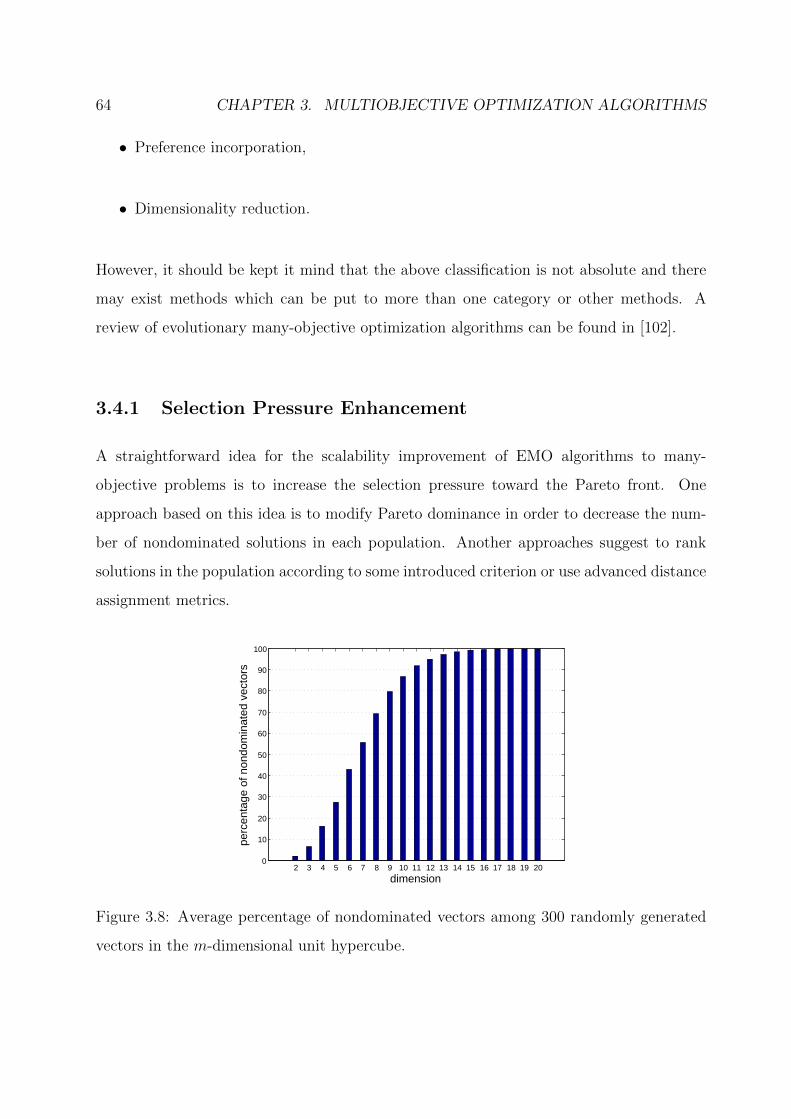
64 CHAPTER 3. MULTIOBJECTIVE OPTIMIZATION ALGORITHMS
• Preference incorporation,
• Dimensionality reduction.
However, it should be kept it mind that the above classification is not absolute and there
may exist methods which can be put to more than one category or other methods. A
review of evolutionary many-objective optimization algorithms can be found in [102].
3.4.1 Selection Pressure Enhancement
A straightforward idea for the scalability improvement of EMO algorithms to many-
objective problems is to increase the selection pressure toward the Pareto front. One
approach based on this idea is to modify Pareto dominance in order to decrease the num-
ber of nondominated solutions in each population. Another approaches suggest to rank
solutions in the population according to some introduced criterion or use advanced distance
assignment metrics.
2 3 4 5 6 7 8 9 10 11 12 13 14 15 16 17 18 19 200
10
20
30
40
50
60
70
80
90
100
dimension
perc
enta
ge o
f non
dom
inat
ed v
ecto
rs
Figure 3.8: Average percentage of nondominated vectors among 300 randomly generated
vectors in the m-dimensional unit hypercube.

3.4. EVOLUTIONARY MANY-OBJECTIVE OPTIMIZATION ALGORITHMS 65
Modification of Pareto Dominance
Sato et al. [152] demonstrated that the use of a modified dominance, instead of the stan-
dard Pareto dominance, clearly improved the performance of NSGA-II for many-objective
problems. In order to increase the selection pressure toward the Pareto front by the Pareto
sorting in NSGA-II, they modified Pareto dominance by widening the angle of the dom-
inance region. In this manner, the selection pressure toward the Pareto front can be
strengthened because the number of nondominated solutions in each population is de-
creased by the use of the modified dominance. The angle which extends the dominated
region should be adjusted to the number of objectives. Roughly speaking, the increase in
the number of objectives requires a wider angle of the dominated region.
Modification of Rank Definition
Drechsler et al. [60] proposed the use of a relation called favour to differentiate between
nondominated solutions for the handling of many-objective problems. They defined the
relation favour based on the number of objectives for which one solution is better than the
other. More specifically, a solution x is viewed as being better than another solution y if x
is better than y on more objectives than on which y is better than x. The relation favour
can be defined as follows:
|i : fi(x) < fi(y), 1 ≤ i ≤ m| < |j : fj(y) < fj(x), 1 ≤ j ≤ m|.
The relation favour was modified in Sulflow et al. [168] by taking into account not
only the number of objectives for which one solution is better than the other but also the
difference in objective values between the two solutions.
On the other hand, Kukkonen and Lampinen [117] studied two different aggregation
functions based on the ranks of solutions in terms of each separate objective. One fitness
function uses the sum of ranks for each objective while the other uses the minimum rank
among objectives. To maintain the diversity of the solutions, a linearly increasing diver-
sity maintenance scheme is proposed. At the first generation, the population of the next

66 CHAPTER 3. MULTIOBJECTIVE OPTIMIZATION ALGORITHMS
generation is selected from the combined parent and child population just based on the
ranking-dominance relation. In the half of generations, half of the population of the next
generation is selected based on the ranking-dominance relation from the combined parent
and child population. The rest half of the population is filled with the best members
according to diversity from the remaining individuals of the combined parent and child
population. At the final generation, individuals from the combined parent and child popu-
lation are selected just according to diversity. Experimental results indicated that in some
cases the selection based on ranking-dominance is able to advance the search towards the
Pareto front better than the selection based on Pareto dominance. However, in some cases
it is also possible that the search does not proceed into the direction of the Pareto front
because the ranking-dominance relation permits deterioration of individual objectives.
Corne and Knowles [32] compared various ranking methods with each other. They
reported that the best results were obtained from a simple average ranking method than
from more complicated ranking schemes. In the average ranking method, first a rank for
each objective is assigned to each solution based on the ranking of its objective value for the
corresponding objective among nondominated solutions in the current population. Thus
each solution has M ranks, each of which is based on one of the M objectives. Then the
average rank is calculated for each solution as its rank.
Substitute Distance Metrics
Koppen and Yoshida [114] discussed various substitute distance assignment schemes which
are used to replace the crowding distance assignment in NSGA-II. These distances are based
on measurement procedures for the highest degree, to which a solution is nearly Pareto
dominated by any other solution: like the number of smaller objectives, the magnitude
of all smaller or larger objectives, or a multi-criterion derived from the former ones. The
following four measurements were considered.
Given two solutions A and B, the subvector dominance procedure svd(A,B) counts the
number of objectives of B that are smaller than the corresponding objectives in A. For
3.4. EVOLUTIONARY MANY-OBJECTIVE OPTIMIZATION ALGORITHMS 67
each solution I[i] in a set I of solutions, the largest such value among all other solutions
is assigned as distance value to I[i]. The smaller this value, the smaller is the number of
lower objectives that appear among all other members of the set I. Such a solution is more
close to being not Pareto dominated by any other solution.
On the other hand, the epsilon dominance procedure mepsd(A,B) considers all objec-
tives of B that are larger than the corresponding objectives of A. It computes the smallest
value ε, which, if subtracted from all objectives of B, makes B Pareto dominating A. For
each solution I[i] in a set I of solutions, the smallest such value among all other solutions
is assigned as distance value to I[i]. The larger this distance for a solution, the higher the
effort that would be needed to make the other solutions Pareto dominating the former.
The fuzzy Pareto dominance procedure fuses all the magnitudes of larger objectives into
a single value, instead of seeking the maximum difference. It uses the notion of bounded
division of two reals x and y from [0, 1]:
x
y=
1, if y ≤ x
x/y, if x < y.
All bounded quotients of corresponding objectives in A and B are multiplied. For a smaller
objective in B, this gives a factor of 1. For each solution I[i] in a set I of solutions, the
largest product value from all other solutions is assigned as distance value to I[i]. The
smaller this value, the lower the degree by which a solution is dominated by any other
solution in I.
The subobjective dominance count (SOD-CNT) procedure performs a multi-criterion
ranking, where the number of larger objectives as well as its magnitude are considered.
Taking a solution A of a nondominated solution set I, a set SA of all pairs of two single-
criterion distance measures (svd(A,B) and mepsd(A,B) were used) to all other solutions
B of the set is derived. This set SA has a Pareto set, which is composed of all solutions
that perform well against A. Each solution in I gets the number of occurrences in all the
possible Pareto sets assigned. The higher this number, the more often the corresponding
solution performs well against some other solution in I.

68 CHAPTER 3. MULTIOBJECTIVE OPTIMIZATION ALGORITHMS
For a number of many-objective test problems, all proposed substitute distance assign-
ments resulted into a strongly improved performance of NSGA-II. Based on the analysis
of the obtained results, the authors outlined two promising strategies for the application
of NSGA-II to many-objective optimization problems: first is to replace the crowding dis-
tance completely by the epsilon dominance distance, second is to use the sub-objective
dominance count distance for the first generations of the algorithm, as long as most of the
individuals get rank 1 assigned, and switch to the crowding distance, once the SOD-CNT
values tend to be equalized over the whole population.
3.4.2 Different Fitness Assignment Schemes
Another idea for the scalability improvement of EMO algorithms is the use of different
fitness evaluation mechanisms instead of the Pareto dominance. One approach is to use
a number of different scalarizing functions for fitness evaluation. Another approach based
on this idea is the use of indicator-based evolutionary algorithms where indicator functions
such as hypervolume are used to evaluate each solution.
Scalarizing-Based Fitness Assignment
Converting a multiobjective problem into a single-objective one by using different scalariz-
ing functions is the basic idea behind many traditional mathematical programming meth-
ods for approximating the Pareto front. The main advantage of the use of scalarizing
functions for many-objective problems is their efficiency. For example, weighted sums of
multiple objectives can be easily calculated even when the number of objectives is large. On
the other hand, the computation time for hypervolume calculation exponentially increases
with the number of objectives.
In [91], there was shown that the use of many single objective optimizations based on
aggregation functions is more effective than the use of a Pareto-ranking based optimizers
on many-objective problems. However, the more efficient way is to use the ranking strategy
based on the aggregation methods in the the single run of a multiobjective optimizer then

3.4. EVOLUTIONARY MANY-OBJECTIVE OPTIMIZATION ALGORITHMS 69
performing multiple runs of a single objective optimizer.
Hughes [90] proposed non-Pareto evolutionary multiobjective algorithm, called multiple
single objective Pareto sampling (MSOPS). At every generation, the algorithm uses a set
of target vectors to evaluate the performance of every individual in the population based on
the chosen aggregation method. Thus, each member of the population has a set of scores
that indicate how well the population member performs on each scalarizing function. The
scores are held in a score matrix, which is ranked, with the best performing population
member on the corresponding target vector being given a rank of 1, and the worst a rank
of P . The rank values are stored in a rank matrix whose rows are sorted, with the ranks
for each population member placed in ascending order. Then the rank matrix is used to
rank the population, with the most fit being the solution that achieved the most scores
which were ranked 1.
In [92], there was proposed the improved version of MSOPS, called MSOPS-II. In this
work, two extensions are used compared to the previous work. The first provides automatic
target vector generation, removing the requirement for initial a-priori designer intervention;
and secondly redefines the fitness assignment method to simplify analysis and allow more
comprehensive constraint handling. The significant enhancements allow the new MSOPS-II
ranking process to be used as part of a general-purpose multi/many objective optimization
algorithm, requiring minimal initial configuration.
In [93], Hughes proposed an algorithm for many-objective optimization. The algorithm
is based on the same strategy as MSOPS [90] and MSOPS-II [92], which use a set of target
vectors to direct and control the search process. Each target vector is coupled with at
least one aggregation function that turns each objective vector into a scalar value for use
in the optimization process. The algorithm operates by treating each target vector and
associated aggregation function as a single-objective optimization process and tracks the
parameter vector that best optimizes the aggregated objective values in the target vector
direction. At each iteration, one target vector is chosen at random and its corresponding
parameter vector is utilized to the line search. All points evaluated as part of line search
are stored and used to update the population.

70 CHAPTER 3. MULTIOBJECTIVE OPTIMIZATION ALGORITHMS
Ishibuchi et al. [97] proposed a hybrid algorithm, which employees an idea of probabilis-
tically using a scalarizing fitness function in evolutionary multiobjective optimization. The
authors used the NSGA-II algorithmic framework introducing two probabilities to specify
how often the scalarizing fitness function is used for parent selection and generation update
in the algorithms. When a pair of parent solutions are to be selected from the current pop-
ulation, the weighted sum fitness function and the NSGA-II fitness evaluation mechanism
are used with the probabilities PPS and (1− PPS), respectively. As in the parent selection
phase, the weighted sum fitness function is probabilistically used in the generation update
phase. When one solution is to be chosen from the enlarged population and added to the
next population, the weighted sum fitness function and the NSGA-II fitness evaluation
mechanism are used with the probabilities PGU and (1 − PGU), respectively. The compu-
tational experiments on multiobjective 0/1 knapsack problems showed that the proposed
approach improves the performance of EMO algorithms.
Moreover, the scalarizing fitness functions were also used in other studies [98, 99,
103, 105]. Its use proved to be an efficient and effective way for fitness assignment in
EMO algorithms. Furthermore, the scalarizing fitness assignment mechanism is used in
MOEA/D, which was discussed in more detail in the previous section. In some recent
studies, MOEA/D has been also applied to many-objective problems producing a good
performance with the increasing number of objectives [44, 154].
Indicator-Based Fitness Assignment
A number of performance indicators have been proposed to quantitatively measure and
compare the quality of outcomes produced by EMO algorithms. Assuming that a perfor-
mance indicator provides a good ordering among sets that represent Pareto approximations,
the fitness function used to select individuals may be defined in such a way that the chosen
indicator is optimized. In fact, in recent years a trend can be observed to directly use
specific measures such as the hypervolume indicator and the epsilon indicator to guide
the search. The hypervolume is a popular performance evaluation measure but it was

3.4. EVOLUTIONARY MANY-OBJECTIVE OPTIMIZATION ALGORITHMS 71
rarely used until recently. This fact may be mostly explained by the complexity of the
hypervolume calculation in terms of programming and computation time. However, theo-
retical studies [68, 203] showed that it is the only indicator known to be strictly monotonic
with respect to Pareto dominance and thereby guaranteeing that the Pareto optimal front
achieves the maximum hypervolume possible, while any worse set will be assigned a worse
indicator value.
Several variants of indicator-based evolutionary algorithms have been proposed in the
literature. In those variants, the hypervolume was almost always used as an indica-
tor. However, the difficulty in the application of hypervolume-based algorithms to many-
objective problem is a large computation cost for the hypervolume calculation. Knowles
and Corne [110] were the first to propose the integration of the hypervolume indicator into
the optimization process. In particular, they described an adaptive archiving algorithm to
maintain a separate, bounded archive of nondominated solutions based on the hypervolume
indicator.
Huband et al. [89] presented MOEA, which includes a modified SPEA2 environmental
selection procedure, where a hypervolume-related measure replaces the original density
estimation technique. They involved the product of the one-dimensional lengths to the
next worse objective function value in the front for each objective as selection criterion
in case of equal fitness values. In the two-objective case, this exactly corresponds to
the S metric contribution. In case of more than two objectives, this procedure provides
only a lower bound of the hypervolume value. They presented an evolution strategy with
probabilistic mutation (ESP). It extends traditional evolution strategies in two principal
ways: ESP applies mutation probabilistically in a GA-like fashion, and it uses a new
hypervolume-based, parameterless, scaling independent measure for resolving ties during
the selection process.
A general framework of indicator-based evolutionary algorithm (IBEA) was proposed
by Zitzler and S. Kunzli [198]. This approach can use an arbitrary indicator to compare
a pair of candidate solutions, in their work authors consider the epsilon and hypervolume
indicators. In the IBEA, any additional diversity preservation mechanism such as fitness
72 CHAPTER 3. MULTIOBJECTIVE OPTIMIZATION ALGORITHMS
sharing is no longer required. In comparison to other EMO algorithms, the IBEA only
compares pairs of individuals instead of entire approximation sets. A scheme similar to
summing up the indicator values for each population member with respect to the rest of
population is used to assign the fitness for each individual in the population. Binary tour-
nament selection is performed in order to fill the temporary mating pool. Then, variation
operators are applied to generate a set of offspring. Environmental selection is performed
by iteratively removing from the combined population of parents and offspring a solution
with the smallest fitness value and recalculating the fitness of the remaining individuals.
Wagner et al. [184] reported good results by IBEA for many-objective problems. Since
IBEA does not use Pareto dominance, its search ability is not severely deteriorated by
the increase in the number of objectives. Ishibuchi et al. [101] proposed an iterative ver-
sion of IBEA to decrease the computation cost by searching for only a small number of
representative solutions. For the same purpose, Brockhoff and Zitzler [19, 20] examined
dimensionality reduction in indicator-based evolutionary algorithms.
Emmerich et al. [64] and Beume et al. [13] suggested an EMO algorithm adapted specif-
ically to the hypervolume indicator, called S metric selection evolutionary multiobjective
algorithm (SMS-EMOA). It was the first EMO algorithm aiming explicitly at the maxi-
mization of the dominated hypervolume within the optimization process. Moreover, the
proposed algorithm is the first steady-state evolutionary algorithm for multiobjective op-
timization. SMS-EMOA features a selection operator based on the hypervolume measure
combined with the concept of nondominated sorting. The algorithm’s population evolves
to a well-distributed set of solutions, thereby focussing on interesting regions of the Pareto
front. The algorithm was compared with state-of-the-art EMO algorithms on two and
three-objective benchmark suites as well as on aeronautical real-world applications pro-
viding superior performance in terms of the hypervolume indicator. Furthermore, a fast
algorithm for the calculation of the contributing hypervolume for three-dimensional case
is suggested in [13].
Bader et al. [6] proposed a method to calculate the contributing hypervolume of so-
lutions in the population using Monte Carlo simulation. The proposed procedure works

3.4. EVOLUTIONARY MANY-OBJECTIVE OPTIMIZATION ALGORITHMS 73
in two steps. First, a number of points are sampled within a hyperrectangle, next the
number of hits is calculated and the hypervolume contribution is evaluated as the hit ratio
multiplied with the volume of the sampling box. Moreover the algorithm uses an adaptive
scheme to reduce the total number of samples as well as a statistical test to determine
the probability that the solution with the smallest contribution has obtained the smallest
contribution estimate [5].
In [7], Bader and Zitzler suggested a fast hypervolume-based EMO algorithm called
HypE. It is a successor of the algorithm proposed in [6]. It also uses a fast method
based on Monte Carlo simulations to estimate the hypervolume value of an approximation
set, however, the entire objective space is utilized to draw samples. Additionally, both its
environmental and mating selection step rely on a new fitness assignment scheme based not
only on the hypervolume contribution, but also on parts of the objective space dominated
by more than one solution. The main idea is not that the actual indicator values are
important, but rather that the rankings of solutions induced by the hypervolume indicator.
Besides the algorithms based on optimizing popular quality indicators, such as the
hypervolume and epsilon indicator, some recent studies suggest approaches which incorpo-
rate other performance metrics. Thus, Bringmann et al. [18] proposed an EMO algorithm
that works with a formal notion of approximation and improves the approximation quality
during its iterative process. In every generation, the algorithm aims at minimizing the
additive approximation of the population with respect to the archive of nondominated
solutions found so far. For each solution in the combined population of parents and off-
spring, the approximation is computed which is the approximation of the set of all solution
except the solution for which the approximation is computed. The individuals with the
smallest such value are iteratively removed. The algorithm produced competitive results
with state-of-the-art algorithms on the set of problems having up to 20 dimensions.
Rodrıguez Villalobos and Coello Coello [148] proposed an EMO algorithm based on
the performance indicator called ∆p. The ∆p indicator consists of GD and IGD metrics
and is viewed as an averaged Hausdorff distance [158]. The algorithm uses the reference
set to approximate the Pareto front of MOP. The selection procedure is solely based on
74 CHAPTER 3. MULTIOBJECTIVE OPTIMIZATION ALGORITHMS
the ∆p indicator. After generating offspring population, the individuals with the lowest
contribution to ∆p are selected from the combined population to form the population of
the next generation.
3.4.3 Use of Preference Information
Besides the difficulty related with the dominance based selection mechanism discussed at
the beginning of this section, there is another difficulty which rises dealing with many-
objective problems. As the number of objectives increases, the objective space becomes
larger. In turn, this requires the exponential increase in the number of nondominated
solutions that are necessary for the approximation of the Pareto front. However, it may
become unacceptably difficult and computationally expensive to process a population with
a larger number of solutions by EMO algorithms which are usually designed to search for
a set of nondominated solutions that approximates the entire Pareto front. Therefore, it
is a good idea to focus on a specific region of the Pareto front using the decision makers
preference. In the following, we briefly discuss some studies where the preference informa-
tion is incorporated in EMO algorithms in order to concentrate on a small region of the
Pareto front handling high-dimensional objective space.
Fleming et al. [69] described a preference articulation method to many-objective prob-
lems where the focused region gradually becomes smaller during the evolutionary process.
The parallel coordinates representation is used after a number of generations to represent
the population to the decision maker. After analyzing the plots, some of the objectives
are converted to be constraints. The values are constrained to the worst solution for that
objective shown on the plot. Thereafter, the optimizer is released to cycle through more
generations. After that, the process of isolating the best solution and converting its objec-
tive into a constraint is repeated. In this way, the search is progressively concentrated on
the desirable objectives at the same time optimizing them until a very small set of solutions
is obtained.
Deb and Sundar [49] incorporated reference point-based preference information into

3.4. EVOLUTIONARY MANY-OBJECTIVE OPTIMIZATION ALGORITHMS 75
NSGA-II. In their approach, the normalized distance to a reference point is taken into
account to evaluate each solution after Pareto sorting. This means that the normalized
distance is used as a secondary criterion instead of the crowding distance in NSGA-II.
A number of nondominated solutions are obtained around the reference point. Multiple
reference points can be handled to explore the decision maker’s preferred regions of the
Pareto front.
Thiele et al. [173] used reference point-based preference information in IBEA. First a
rough approximation of the Pareto front is obtained. Such a rough approximation is used
by the decision maker to specify a reference point. Then IBEA searches for a number of
nondominated solutions around the reference point. The focus of the multiobjective search
by IBEA can be controlled using a parameter value and a reference point. Usually, the
focused region gradually becomes smaller through the interaction with the decision maker.
The use of preference information is based on a similar idea to weighted integration in [196].
In the abovementioned methods, preference information is used to focus on a specific region
in the high-dimensional objective space with many objectives while EMO algorithms are
used to search for a number of nondominated solutions in such a focused region.
Deb and Jain [44] suggested a reference-point based many-objective NSGA-II, called
MO-NSGA-II. MO-NSGA-II emphasizes population members which are nondominated yet
close to a set of well-distributed reference points. The basic framework of MO-NSGA-II
remains similar to the original NSGA-II, but significant changes were made in the selection
mechanism. At every generation, MO-NSGA-II builds a hyper-plane on which a predefined
set of evenly distributed reference points is generated. Then, the population members
from the last nondominated front being retained to the next generation are projected
to the constructed hyperplane and associated with a reference point that is closest to
the projected solution. The diversity among obtained solutions is ensured by emphasizing
population members which form less-crowded clusters around each reference point. During
the parent selection procedure, when two solutions from the same nondominated front are
compared the one which is associated with less-represented reference point is preferable.
MO-NSGA-II showed a good performance on problems having up to 10 objectives.

76 CHAPTER 3. MULTIOBJECTIVE OPTIMIZATION ALGORITHMS
3.4.4 Dimensionality Reduction
Another approach for dealing with many-objective problems is dimensionality reduction.
These approaches assume the existence of redundant objectives in a given many-objective
problem. Operating on the objective vectors of the nondominated solutions obtained from
an EMO algorithm, these approaches aim to identify a smallest set of conflicting objectives
which: (i) generates the same Pareto front as the original problem, or (ii) alternatively,
preserves the dominance relations of the original problem. Such objectives are termed as
essential and the remaining ones as redundant. Dimensionality reduction, always when
it is possible, can remedy virtually all difficulties related with many-objective problems,
namely it will contribute to higher search efficiency, lower computational cost and ease in
visualization and decision-making.
Dimensionality reduction approaches can be classified into linear and nonlinear ap-
proaches. Furthermore, it may be referred to online or offline reduction method depending
on whether it is performed during an EMO algorithm run to simplify the search or post
EMO algorithm run to assist in the decision making, respectively.
Saxena and Deb [47] proposed dimensionality reduction method based on principal
component analysis (PCA). In their proposal, referred as PCA-NSGA-II, a representative
set of solutions for dimensionality analysis is obtained by running NSGA-II for a large
number of generations. Thereafter, the correlation matrix R, with respect to the objec-
tives, is computed using the objective values of the final population. The eigenvalues and
corresponding eigenvectors are then analyzed in order to reduce the objectives. The proce-
dure starts with the original set of objectives, and the objectives are eliminated iteratively,
based on their contribution to the principal components and the degree of their conflict
with the other objectives. Once the set of objectives cannot be reduced further, the proce-
dure is stopped and the reduced set of objectives is declared. However, the proposed linear
PCA technique has a drawback of misinterpreting the data when it lies on submanifolds.
To mitigate the difficulties related to the use of linear PCA for dimensionality reduc-
tion, Saxena and Deb [153] suggested nonlinear dimensionality reduction-based techniques.

3.4. EVOLUTIONARY MANY-OBJECTIVE OPTIMIZATION ALGORITHMS 77
While the reduction procedure remained largely the same as in [47], the key difference lay
in the way the correlation was calculated. Instead of the linear PCA, two new proposals
were made: correntropy PCA (C-PCA) and maximum variance unfolding (MVU). The
corresponding algorithms were named C-PCA-NSGA-II and MVU-PCA-NSGA-II. Using
these nonlinear techniques, more accurate results were obtained for up to 50-objective
DTLZ5-(2,M) problems. Even so, the algorithms were found to be ineffective on a number
of other problems, such as DTLZ5-(5,10) and DTLZ5-(5,20), since the population for di-
mensionality analysis was not converged near enough to the Pareto front for a meaningful
analysis.
The dimensionality reduction approach proposed in [21] is based on preserving the
dominance relations in the given nondominated solutions. For a given objective set F , if
the dominance relations among the objective vectors remains unchanged when an objective
f ∈ F is removed, then f is considered to be nonconflicting with the other objectives in F .
Based on this criterion, an exact and a greedy algorithm is proposed to address δ-MOSS,
finding the minimum objective subset corresponding to a given error δ and k-EMOSS,
finding an objective subset of size k with minimum possible error problems. However, due
to the underlying assumptions, this approach is limited to linear objective reduction and
equally distributed solutions in the objective space.
Lopez Jaimes et al. [127] have developed a dimensionality reduction scheme based on
an unsupervised feature selection technique. In their approach, the objective set is first
divided into homogeneous neighborhoods based on a correlation matrix of a nondominated
set obtained using an evolutionary algorithm. The conflict between the objectives takes
role of a distance, meaning the more conflict between the objectives, the more distant
they are in the objective conflict space. Thereafter, the most compact neighborhood is
chosen, and all the objectives in it except the center one are dropped, as they are the least
conflicting.
Singh et al. [162] proposed Pareto corner search evolutionary algorithm (PCSEA). The
algorithm searches for only the corners of the Pareto optimal front instead of aiming for
the complete PF. The solutions so obtained are assumed to appropriately capture the
78 CHAPTER 3. MULTIOBJECTIVE OPTIMIZATION ALGORITHMS
dependency of PF on different objectives. To find the corners solutions, PCSEA uses
corner-sort ranking procedure. The solutions are sorted based on the increasing individual
objective values and increasing all-but-one objective, converted to a single composite value
using L2 norm values. Then, dimensionality reduction procedure is performed. It is based
on the premise that omitting a redundant and an essential objective will have negligible and
substantial effect, respectively, on the number of nondominated solutions in the population.
Starting from the first objective, each objective is dropped in turn, and the change in the
number of nondominated solutions is observed. If the ratio between resulting nondominated
solutions and the reference set exceeds a user-defined threshold, then the objective is
deemed redundant and removed. However, there are a number of limitations related to the
method due to the use of corner solutions only to identify dimensionality. The resulting
set may not be able to capture the entire information regarding the conflict in the Pareto
front, there also may be the situation where certain objectives do not contribute to the
extremities of the Pareto front, but contribute elsewhere.
3.5 Summary
The goal of multiobjective optimization to approximate the Pareto set is dual in nature,
it requires obtaining a set of solutions as close as possible to the true Pareto optimal
set and, at the same time, as diverse as possible. Algorithms for solving multiobjective
optimization problems must be able to satisfy this two goals. This chapter reviews a
number of approaches designed to perform this task.
The majority of classical methods treat multiobjective optimization in the same way as
single-objective optimization. They avoid the complexity induced by the presence of multi-
ple objectives by converting a multiobjective optimization problem into a single-objective
optimization problem with a real-valued objective function. This approach is referred
to as scalarization, and the function that depends on user-defined parameters is termed
the scalarizing function. In summary, the weighted sum method consists in minimizing
a weighted sum of multiple objectives; ε-constraint method suggests optimizing one ob-

3.5. SUMMARY 79
jective function imposing all other objectives as constraints; weighted metric methods are
based on minimizing an Lp metric constructed from all objectives. The normal boundary
intersection method suggests maximizing the distance along the normal vector towards
the origin from a point on the constructed hyper plane satisfying additional equality con-
straint. Finally, the normal constraint method provides the reduction of the feasible region
by imposing additional constraints and optimizing one objective.
All these methods result in a single-objective optimization problem, which must be
solved using a single-objective optimization algorithm. In most cases, the optimal solution
to the single-objective optimization problem is expected to be a Pareto optimal solution.
Such a solution is specific to the parameters used in the conversion method. To find
different Pareto optimal solutions, the parameters must be changed and the resulting new
single-objective optimization problem has to be solved again. On the other hand, Timmel’s
method is a population-based stochastic approach, hence it does not require multiple runs
with different parameter settings. It is expected to find the approximation to the Pareto
optimal set in a single run. Its stochastic nature to generate new solutions and the use of
a population of solutions instead of a single one represent philosophy similar to that used
in evolutionary algorithms. However, it does not employ any specific strategy to provide
the diversity among the obtained solutions. In turn, other classical methods rely on the
uniformly distributed set of weight vector to achieve the diversity of the obtained solutions
or on the value of ε in the case of the ε-constrained method.
Despite the simplicity of use and good theoretical properties, there are some limitations
related to the classical methods. In particular, some algorithms do not guarantee finding
solutions in the entire Pareto optimal region after performing a number of single-objective
optimizations. Thus, the weighted sum method and the weighted metric method with small
p have limitations in finding solutions in the nonconvex region of the Pareto optimal front.
Furthermore, some methods require additional knowledge about the problem that must
be provided in advance. Thus, the weighted metric method uses a reference point. The
normal boundary intersection method and the normal constraint method use the anchor
points to convert a multiobjective problem into a single-objective optimization problem.

80 CHAPTER 3. MULTIOBJECTIVE OPTIMIZATION ALGORITHMS
The main limitation of Timmel’s method is the use of the gradients of objectives to generate
new solutions. This requires all objectives in the multiobjective optimization problem to
be differentiable. However, Timmel’s method can find Pareto optimal solutions in both
convex and nonconvex regions of the Pareto front.
Contrarily to the majority of classical methods, evolutionary algorithms are population-
based optimization techniques. This feature makes them particularly suitable for solving
multiobjective optimization problems. The main aspects to be taken into consideration
when implementing MOEAs are: (i) fitness assignment, (ii) diversity preservation, and (iii)
elitism. Although the discussed algorithms are organized on the basis of their variation
operators, one can trace how each of these aspects was included into MOEAs since the first
pioneering studies appeared in the mid 1980s. Regarding the fitness assignment, one can
distinguish the following most popular techniques: dominance-based, scalarizing-based,
and indicator-based fitness assignment. Furthermore, diversity of solutions within the
current Pareto set approximation is maintained by incorporating density information into
the selection process of EMO algorithms. Some widely used diversity preserving methods
are: (i) fitness sharing, (ii) hypergrid, (iii) clustering, (iv) nearest neighbor, (v) crowding
distance. Recently, the use of quality indicators as the diversity estimator has become
very popular. Elitism is addressed to the issue of maintaining good solutions found during
the optimization process. The elite preserving operator is usually included in MOEAs to
make them better convergent to the Pareto front. One way to deal with this problem is to
combine the parent and offspring populations and to apply selection procedure to select a
new population. Alternatively, the external archive can be maintained where the promising
solutions are stored during the search.
The early MOEAs are mostly GA-based non-elitist algorithms. The first multiobjec-
tive evolutionary algorithm is VEGA. During its selection process individuals are selected
into the mating pool based on the particular objective function values. However, it does
not use any diversity technique. Later approaches proposed in the early 1990s (MOGA,
NSGA, etc.) followed the Goldberg’s suggestion of incorporating the concept of the Pareto
dominance in the fitness assignment mechanism during the mating selection. The most
3.5. SUMMARY 81
popular technique, at the time, to maintain the diversity among solutions is based on a
sharing function. The early MOEAs showed the ability to approximate the Pareto set on a
number of test functions and real-world applications, they provided substantial foundations
for developing further generations of MOEAs.
In the early 2000s, the selection using the Pareto dominance-based fitness assignment
became the most popular one. Additionally, the elitism is somehow implemented in almost
all algorithms of that time. Until now, the most popular algorithm framework is the one
used in NSGA-II. NSGA-II carries out a nondominated sorting of a combined population.
The use of the combined population instead of simply replacing the old population by
offspring makes the algorithm an elitist type. The introduced crowding distance is used
to decide which solutions from the last accepted nondominated front are included into the
new population. This operator preserves diversity of solutions in the population. Subse-
quently, a number of single-objective EAs (ES, DE, CMA-ES, etc.) were extended to deal
with multiobjective optimization problems by simply replacing the GA operator in the
NSGA-II framework. These proposals take advantage of their offspring generation opera-
tors adopting the same strategy to guide the search in the objective space. On the other
hand, other algorithms are extended with some modifications. For instance, in MEES the
elitism is implemented in such a way that a specified portion of nondominated solutions is
introduced in the main population from the archive, while the main population contains
mainly offspring produced by the previous population.
However, it is not possible for some single-objective EAs to be extended to deal with
multiple objectives by only modifying their selection operators. For example, PSO requires
to define the notion of the local and global best particles to guide the search of a particle.
In general, this is accomplished using the external archive where the local and global best
solutions are kept. Decision on the selection of the local and global best particles is usually
made using the Pareto dominance relation. Other algorithms use a local search strategy
to approximate the Pareto set. Thus, PAES uses point to point generation strategy, where
one offspring is created and compared with the parent using the dominance relation. In
the case when the parent and offspring are both nondominated with respect to each other,
82 CHAPTER 3. MULTIOBJECTIVE OPTIMIZATION ALGORITHMS
the offspring is compared with the current archive. Once again, decision on acceptance of
offspring is made considering the dominance relation and the density of solutions. More-
over, AMOSA uses SA updating rule to choose the parent of the next generation when an
offspring is dominated by the parent. Furthermore, the presence of the external archive
in these algorithms to store nondominated solutions found during the search ensures the
elitism.
A different class of algorithms from the ones discussed so far is MOEA/D. Contrar-
ily to other considered algorithms, which were developed on the basis of their single-
objective counterparts, MOEA/D was designed specifically to handle multiobjective opti-
mization problems. In MOEA/D, each solution is associated with one scalarizing function.
MOEA/D optimizes multiple subproblems in a single run exploring the information about
fitness landscape of the neighboring subproblems. Different variation operators (GA, DE,
EDA, etc.) can be used to generate offspring individuals. In general, MOEA/D represents
a flexible and powerful algorithmic framework, where such aspects as fitness assignment,
diversity preserving and elitism are implemented through the use of a set of uniformly
distributed weight vectors. Moreover, it can be easily hybridized using local search algo-
rithms.
Although state-of-the-art Pareto dominance-based EMO algorithms usually work well
on two- and three-objective problems, a number of studies in the early 2000s revealed that
their search ability is severely deteriorated when the number of objectives increases. This
weakness of the Pareto dominance-based fitness assignment prompted further research in
the field of many-objective optimization. To improve the scalability of EMO algorithms,
some studies suggest to increase the selection pressure toward the Pareto front modifying
the Pareto dominance relation or assigning different ranks to nondominated solutions. On
the other hand, the decision maker’s preferences can be used during the search in order
to concentrate on preferred regions of the Pareto front. Another idea for the scalability
improvement is to use different fitness assignment mechanisms instead of the Pareto dom-
inance. One approach to accomplish this is to incorporate the quality indicators (such
as the hypervolume and epsilon indicator) in the fitness assignment mechanism. Another

3.5. SUMMARY 83
approach is to use a number of different scalarizing functions for assigning the fitness to
individuals in the population. Another perspective to handling many-objective problems
is to decrease the number of objectives. This approach is based on the notion that not all
objectives are necessary to define the Pareto front. For this purpose, linear and nonlin-
ear correlation-based dimensionality reduction techniques based on principal component
analysis and maximum variance unfolding can be used. On the other hand, dimensionality
reduction can be based on the Pareto dominance.

84 CHAPTER 3. MULTIOBJECTIVE OPTIMIZATION ALGORITHMS

Chapter 4
Performance Assessment of
Multiobjective Optimization
Algorithms
4.1 Introduction
This chapter addresses the issue of performance assessment of different MO algorithms.
Generally, in optimization the notion of performance includes both the quality of the out-
come as well as the computational resources needed to generate this outcome. Concerning
the latter aspect, the number of function evaluations or the overall computing time is
commonly used. In this case, there is no difference between single and multiobjective op-
timization. However, there is a significant difference concerning the aspect related with
the produced outcome. In single-objective optimization, the quality of the outcome can
be defined by means of the objective function value: the smaller the value, the better
performance (assuming minimization). While in multiobjective optimization, the outcome
of the algorithm is usually a set of solutions. In the following, the outcome of a multiob-
jective optimizer is considered as a set of incomparable solutions, which is denoted as an
approximation set. In terms of the objective space, this can be formalized as follows [204].
85

86 CHAPTER 4. PERFORMANCE ASSESSMENT OF MO ALGORITHMS
1f
2f
Pareto optimal
front
(a) Approximation set obtained by Algorithm 1
(convergence is good, distribution is poor)
1f
2f
Pareto optimal
front
(b) Approximation set obtained by Algorithm 2
(convergence is poor, distribution is good)
Figure 4.1: Performance produced by two algorithms on a same problem.
Definition 4.1.1 (approximation set). Let A ⊆ Rm be a set of objective vectors. A
is called an approximation set if any element of A does not weakly dominate any other
objective vector in A. The set of all approximation sets is denoted as Ω.
The motivation behind this definition is that all solutions dominated by any other
solution returned by the optimization algorithm are of no interest, and therefore can be
discarded. Nevertheless, the above definition does not comprise any notion of quality,
while it is obvious that the final goal of an optimization process is not to obtain any
approximation set, but a good approximation set.
As it is mentioned in this thesis, there are two distinct goals in multiobjective opti-
mization. Therefore, there are two primary requirements to any approximation set: (i)
it should be as close as possible to the true Pareto optimal front, and (ii) it should be
as diverse as possible. However, it is not straightforward how to compare, under these
distinct and somewhat conflicting requirements, approximation sets produced by different
algorithms.
The difficulty in comparing two approximation sets can be easily understood observ-
ing Figure 4.1. The figure illustrates two approximation sets obtained by two different
4.2. BENCHMARK PROBLEMS 87
algorithms on the same problem. It can be seen that the approximation set produced by
the first algorithm (Figure 4.1(a)) converges well to the Pareto optimal front, but clearly
there is lack of diversity among solutions. This algorithm has failed to provide information
about the intermediate Pareto optimal region. On the other hand, the second algorithm
(Figure 4.1(b)) has obtained a well distributed set of solutions, but they are not close to
the true Pareto optimal front. Although the latter approximation set can provide a rough
idea of different trade-off solutions, the exact Pareto optimal solutions are not discovered.
So, with such sets of obtained solutions, it is difficult to conclude which approximation set
is better in an absolute sense.
Due to the stochastic nature of evolutionary algorithms, it is common practice to per-
form several runs on a chosen set of test problems in order to assess their performance.
The produced outcomes are quantitatively assessed using quality indicators. Quality indi-
cators can be categorized as follows: (i) first type of indicators measures the convergence
to the Pareto optimal front, (ii) second type of indicators measures the diversity among
the obtained solutions, and (iii) third type of indicators can be used to measure both goals
of multiobjective optimization. The formal definition of quality indicators is provided later
in this chapter. Assigning real values to each approximation set allows to perform common
statistical tests and to obtain quantitative and statistically sound inferences about the
algorithm’s performance.
In the following, this chapter reviews some existing test suites for multiobjective opti-
mization, a number of unary quality indicators and a few statistical comparison methods
that can be used for performance assessment of multiobjective optimizers.
4.2 Benchmark Problems
Benchmark problems are an important aspect of optimization. They are often used for both
assessing the qualities of optimization algorithms and designing new algorithms. Artificially
constructed test problems offer many advantages over real-world problems for the purpose
of general performance testing. Test problems can be designed to be easy to describe,

88 CHAPTER 4. PERFORMANCE ASSESSMENT OF MO ALGORITHMS
easy to understand, easy to implement, fast, and their optima are often known in advance.
This is also true for multiobjective optimization. First multiobjective test problems that
have been designed in the early stages of EMO research are relatively simple. Moreover, in
most problems neither the difficulty caused by such problems for multiobjective algorithms
cannot be controlled nor the dimensionality can be changed. As a result, they are rarely
used nowadays. So, during the last decade a number of publications has appeared in the
corresponding literature where the issue of designing challenging test problems has been
addressed. This section reviews some recent benchmark problems that are widely used for
comparing the performance of EMO algorithms.
Deb [41] first suggested a general methodology for constructing two-objective problems
from single-objective optimization problems. The proposed approach allows known diffi-
cult features of single-objective problems (such as multi-modality, isolation, or deception)
to be directly transferred to the corresponding multiobjective problem. Based on this con-
struction process Zitzler et al. [197] framed six problems, since then they have been widely
used and are known as ZDT test suites.
Furthermore, in order to study the performance of EMO algorithms on problems with
more than two objectives Deb et al. [50] proposed DTLZ test suite. The suggested test
problems, unlike all other earlier multiobjective test problems, are scalable with respect to
the number of parameters as well as the number of objectives. This important characteristic
has facilitated a number of investigations in the field of many-objective optimization. In the
original technical report [50], seven unconstrained (DTLZ1-DTLZ7) and two constrained
(DTLZ8 and DTLZ9) problems were suggested, while later in the conference paper [51]
some of the problems were dropped.
Despite the extensive use of scalable DTLZ test suite in many EMO studies, it has
been very often criticized for being too simple and due to its limitations. Specifically,
none of its problems is deceptive, none of its problems is non-separable, and the number of
position parameters is always fixed relative to the number of objectives. Moreover, DTLZ5
and DTLZ6 do not behave as expected, their Pareto fronts are unclear beyond three-
objectives [87]. So, Huband et al. [87, 88] proposed a toolkit for creating problems with an

4.2. BENCHMARK PROBLEMS 89
arbitrary number of objectives, where desirable features can easily be incorporated. The
proposed WFG toolkit defines a problem in terms of an underlying vector of parameters
x. The vector x is associated with a simple underlying problem that defines the fitness
space. The vector x is derived, via a series of transition vectors, from a vector of working
parameters z. Each transition vector adds complexity to the underlying problem. The
WFG toolkit allows a user to control, via a series of composable transformations, which
features will be present in the test problem. To create a problem, the user selects several
shape functions to determine the geometry of the fitness space, and employs a number
transformation functions that facilitate the creation of transition vectors. A number of
shape and transition functions were suggested. Additionally, the authors proposed nine test
problems (WFG1-WFG9) that possess some of the pertinent problem characteristics, some
of of them are nonseparable, multimodal, deceptive problems and with different geometry
of the Pareto front. Moreover, all problems are scalable objective- and parameter-wise,
where the number of position- and distance-related parameters can be controlled by the
user.
Deb et al. [48] addressed the issue of developing multiobjective test problems which
introduce controllable linkages among variables using ZDT and DTLZ test problems. The
authors studied three types of variable linkage: (i) linkages among variables affecting ei-
ther the convergence or diversity individually, (ii) linkages among all variables causing a
simultaneous effect in both convergence and maintenance of diversity among solutions, and
(iii) linkages which are non-linear, causing linear operators to face difficulty in preserving
optimality of solutions.
In [177], 19 multiobjective test problems are described, including two-objective, three-
objective, and five-objective problems. The major part of the proposed test suite is
constructed from the known benchmark functions. Thus, some of ZDT and DTLZ test
functions were shifted or rotated thereby adding additional complexity and overcoming
problems related with the original functions. The resulting test suite presents a variety
of difficulties to EMO algorithms and was used in the CEC 2007 Special Session and
Competition.

90 CHAPTER 4. PERFORMANCE ASSESSMENT OF MO ALGORITHMS
Li and Zhang [123] introduced a general class of continuous multiobjective optimization
test instances with arbitrarily prescribed Pareto set shapes. Like DTLZ and WFG test
suites, the proposed test suite uses component functions for defining its Pareto front and
introducing multimodality. Its major advantage over others is that the Pareto set can
be easily prescribed. The authors proposed nine challenged problems with complicated
Pareto set shapes, which take challenges to many MOEAs. Moreover, in the CEC 2009
Special Session and Competition, unconstrained and constrained test functions are designed
with complicated Pareto set shapes [143]. Furthermore, Saxena et al. [155] extended the
framework of constructing test instances with controlling Pareto sets to the case of four
and more objectives.
Moreover, a number of multiobjective test problems were suggested for performance
comparison of MOEAs in different studies [65, 94, 138, 191, 193]. In turn, the paper [67]
addresses the issue of developing dynamic multiobjective test problems by suggesting a
baseline algorithm. A suite of five test problems offering different patterns of changing the
Pareto front with time and different difficulties in tracking the dynamic Pareto optimal
front are presented. Additionaly, a review of so-called classical multiobjective test problems
can be found in [29, 88].
4.3 Quality Indicators
Various quality indicators for measuring the quality of approximation sets have been pro-
posed to compare the performance of different multiobjective optimization algorithms.
Some aim at measuring the distance of an approximation set to the Pareto optimal front.
Other indicators try to capture the diversity of an approximation set. However, some of
the quality indicators are able to measure the convergence to the true Pareto optimal front
as well as diversity of solutions in an approximation set. Generally speaking, it can be
stated that quality indicators map approximation sets to the set of real numbers. The
following definition formalizes this notion as stated in [204].

4.3. QUALITY INDICATORS 91
Definition 4.3.1 (quality indicator). A unary quality indicator is a function I : Ω 7→ R
that assigns each approximation set a real number.
The underlying idea behind the use of the quality indicators is to quantify quality
differences between approximation sets by applying common metrics to the resulting real
numbers. The indicators can be either unary or binary quality indicators; however, in
principle, a quality indicator can take an arbitrary number of arguments. In the following,
all indicators are categorized into three categories, and only the unary quality indicators
are presented.
4.3.1 Indicators Evaluating Convergence
The indicators presented in this section explicitly compute a measure of the closeness of an
approximation set A from the Pareto optimal front PF . They provide a good estimate of
convergence if a large set for PF is chosen. On the one hand, in some problems, the Pareto
front may be known and a set of finite Pareto optimal solutions can be computed. On the
other hand, when the Pareto front is not known, a reference set can be used instead.
Error Ratio Indicator
The error ratio indicator was proposed by Veldhuizen [179] to indicate the percentage of
solutions from an approximation set A that are not members of the Pareto front PF . This
indicator is defined as:
IER =
|A|∑i=1
ei
|A|(4.3.1)
where ei = 0 if vector i is a member of PF , and ei = 1 otherwise. It is clear that
IER = 0 indicates an ideal behavior, since it would mean that all vectors generated by
a multiobjective optimizer belong to PF . It should be noted that this metric requires
knowing the number of elements of the Pareto optimal front, which is often impossible to
determine.

92 CHAPTER 4. PERFORMANCE ASSESSMENT OF MO ALGORITHMS
Maximum Pareto Front Error Indicator
The maximum Pareto front error indicator was suggested by Veldhuizen [179] and deter-
mines a maximum error band which when considered with respect to an approximation set
A = a1, . . . ,a|A| encompasses every vector in the Pareto front PF = a′1, . . . ,a′|PF|.
Stating otherwise, this is the largest minimum distance between each vector in A and the
corresponding closest vector in PF . This indicator is defined as:
IME = maxk
minn
(m∑i=1
∣∣ani − a′ki ∣∣p) 1
p
(4.3.2)
where n = 1, . . . , |A|, k = 1, . . . , |PF|, m is the number of objectives, and p = 2. A result
of 0 indicates A ⊆ PF , any other value indicates at least one vector in A is not in PF .
Generational Distance Indicator
The generational distance (GD) indicator was introduced by Veldhuizen and Lamont [180]
as a way of estimating how far are the elements in an approximation set A from those in
the Pareto front PF and is defined as:
IGD =
(|A|∑i=1
dpi
) 1p
|A|(4.3.3)
where di is the Euclidean distance from i-th point in an approximation set A to its nearest
member of the Pareto optimal front PF .
Set Coverage Indicator
The set coverage indicator was proposed by Zitzler [?] for comparing the performance of two
algorithms by calculating the proportion of solutions in an approximation set produced by
one algorithm which are weakly dominated by solutions in an approximation set produced
by another algorithm. However, if a reference set R is used, this indicator will determine
the proportion of solutions in an approximation set A, which are weakly dominated by
4.3. QUALITY INDICATORS 93
members of R. Thus, this indicator is defined as:
ISC =|a ∈ A | ∃a′ ∈ R : a′ a|
|A|. (4.3.4)
The value ISC = 1 means that all members of A are weakly dominated by R, so smaller
values of ISC are preferable.
Epsilon Indicator
The unary additive ε-indicator was suggested by Zitzler et al. [204]. It is based on the
concept of additive ε-dominance [120] and defined with respect to a reference set R as:
Iε = infε∈R∀a′ ∈ R ∃a ∈ A : a ε a′. (4.3.5)
The ε-indicator gives the minimum factor ε such that any objective vector in R is ε-
dominated by at least one objective vector in A. Smaller values of Iε are preferable.
4.3.2 Indicators Evaluating Diversity
In the following, a few quality indicators are presented that are used to measure how the
second goal of multiobjective optimization is achieved. These indicators quantitatively
assess the diversity among obtained nondominated solutions.
Overall Nondominated Vector Generation Indicator
This indicator introduced by Veldhuizen [179] measures the total number of nondominated
vectors found during MOEA execution and is defined as:
IONV G = |A|. (4.3.6)
Although counting the number of nondominated solutions gives some feeling for how ef-
fective a multiobjective optimizer is in generating desired solutions, it does not reflect on
how far from PF the vectors in A are neither how well the solutions in A are distributed.
There are a few special cases where this indicator can be used to assess the quality of
an approximation set, for example, if the entire search space contains only nondominated
points.

94 CHAPTER 4. PERFORMANCE ASSESSMENT OF MO ALGORITHMS
Spacing Indicator
The spacing indicator was suggested by Schott [157], and it is used to calculate a relative
distance measure between consecutive solutions in an approximation setA = a1, . . . ,a|A|.
This indicator is defined as:
ISS =
√√√√√ |A|∑n=1
(dn − d)2
|A|(4.3.7)
where
dn = mink∈A∧k 6=n
m∑i=1
|ani − aki |
and d is the mean value of the above distance measure
d =
|A|∑n=1
dn|A|
.
The distance measure is the minimum value of the sum of the absolute difference in objec-
tive function values between the n-th solution and any other solution in the approximation
set. This distance measure is different from the minimum Euclidean distance between two
solutions.
Spread Indicator
The spread indicator proposed by Deb et al. [46] measures the extend of spread achieved
among the obtained solutions. This indicator is used to calculate the nonuniformity in the
distribution of the solutions in an approximation set A. The spread indicator is defined
as:
IS =
m∑i=1
dei +|A|−1∑n=1
|dn − d|m∑i=1
dei + (|A| − 1)d(4.3.8)
where dn can be any distance measure between neighboring solutions and d is the mean
value of these distance measures. The Euclidean distance, the sum of the absolute dif-
ferences in objective values or the crowding distance can be used to calculate dn. The

4.3. QUALITY INDICATORS 95
parameter dei is the distance between the extreme solutions of PF and A corresponding to
i-th objective function.
In the case, where there is a large variance in dn, the indicator may be greater than
one. However, a good distribution would make all distances dn equal to d and would
make dei = 0 ∀i ∈ 1, . . . ,m. Thus, for the most widely and uniformly distributed set of
nondominated solutions, the numerator of IS would be zero, making the indicator to take
a value zero. For any other distribution, the value of the metric would be greater than
zero.
In order to use the spread indicator for more then two objectives, Nebro et al. [136]
modified the spread indicator defined in (4.3.8) by computing the distance from a given
point to its nearest neighbor. On the other hand, Custodio et al. [36] proposed a slightly
modified spread indicator, which is defined as follows:
IS = max1≤i≤m
d0,i + d|A|,i +
|A|−1∑n=1
|dn,i − di|
d0,i + d|A|,i + (|A| − 1)di
(4.3.9)
where di, for i = 1, . . . ,m, is the average of the distances dn,i, n = 1, . . . , |A| − 1. The au-
thors report very similar results of their indicator compared to the original spread indicator
defined in [46] for m = 2.
Maximum Spread Indicator
The maximum spread indicator defined by Zitzler [?] measures the length of the diagonal
of a hyperbox formed by the extreme function values observed in an approximation set
A = a1, . . . ,a|A|. This indicator is defined as:
IMS =
√√√√ m∑i=1
(max
1≤n≤|A|ani − min
1≤n≤|A|ani
)2
. (4.3.10)
A normalized version of the maximum spread indicator can be defined as follows:
IMS =
√√√√√ 1
m
m∑i=1
max1≤n≤|A|
ani − min1≤n≤|A|
ani
amaxi − amin
i
2
. (4.3.11)

96 CHAPTER 4. PERFORMANCE ASSESSMENT OF MO ALGORITHMS
where amaxi and amin
i are the maximum and minimum values of the i-th objective in the
approximation set A. In this way, if the maximum spread indicator is one, a widely spread
set of solutions is obtained.
Chi-Square-Like Deviation Indicator
The chi-square-like deviation indicator proposed by Srinivas and Deb [164] is used to es-
timate the distributing ability of multiobjective optimization algorithms. A neighborhood
parameter ε is used to count the number of solutions, nk, within each chosen Pareto opti-
mal solution k ∈ PF . This indicator measures the deviation between this counted set of
numbers with an ideal set in the chi-square sense and is defined as:
ICD =
√√√√|PF|+1∑k=1
(nk − nkσk
)2
. (4.3.12)
Since a uniform distribution is considered as an ideal distribution of solutions in an approx-
imation set, the number of solutions allocated in the niche of each chosen Pareto optimal
solution should be nk = |A|/|PF|. The parameter σ2k = nk(1 − nk/|A|) is suggested for
k = 1, . . . , |PF|. However, the index k = |PF| + 1 represents all solutions which do not
reside in the ε-neighborhood of any of the chosen Pareto optimal solutions. For this index,
the ideal number of solutions and its variance are calculated as follows:
n|PF|+1 = 0, σ2|PF|+1 =
|PF|∑k=1
σ2k = |A|
(1− 1
|PF|
).
Number of Distinct Choices Indicator
The number of distinct choices indicator proposed by Wu and Azarm [188] counts the
number of distinct solutions in a given approximation set A. Each objective is divided
into 1/µ equal divisions, where µ is a user specified number. In this way, the objective
space is divided into (1/µ)m unique, equal-sized m-dimensional hypercubes. Each of the
hypercubes hi, i = 1, . . . , (1/µ)m is referred as the indifference region. Within this region
any two solutions ak,al ∈ A are considered similar to one another. The quantity NT (hi)

4.3. QUALITY INDICATORS 97
will be equal to 1 as long as there is at least one solution in A falling into the indifference
region defined by the hypercube hi. In general, NT (hi) can be stated as:
NT (hi) =
1 ∃ak ∈ A ak ∈ hi0 ∀ak ∈ A ak /∈ hi.
So, this indicator, which is the number of distinct choices for a specified value of µ, is
defined as:
INDC =
(1/µ)m∑i=1
NT (hi). (4.3.13)
Thus, an approximation set A with a higher value of the quantity INDC is preferable.
Cluster Indicator
The number of distinct choices indicator indicates the number of distinct solutions in an
approximation set A, however, it can not properly interpret how clustered these solutions
are. Thus, the cluster indicator [188] can be used to estimate how clustered solutions are.
This indicator is defined as:
ICL =|A|INDC
. (4.3.14)
The value of ICL = 1 would indicate that every solution in |A| is distinct, in all other
cases ICL > 1. Thus, the higher the value of the cluster indicator is, the more clustered an
approximation set A is, and hence the less preferred.
Diversity Indicator
The diversity indicator suggested by Li et al. [124] evaluates the spread of solutions in
an approximation set A considering not only the standard deviation of distances between
solutions in A but also the maximal spread. This indicator is defined as:
IDV =
m∑i=1
(f(max)i − f (min)
i )
1 +
√1|A|
|A|∑k=1
(dk − d)2
(4.3.15)

98 CHAPTER 4. PERFORMANCE ASSESSMENT OF MO ALGORITHMS
where dk is the Euclidean distance between the k-th solution and its closest neighbor, and
d is the mean value of all dk, f(max)i and f
(min)i represents the maximum and minimum
objective function value of i-th objective. The larger value of IDV means a better diversity
of solutions in A.
4.3.3 Indicators Evaluating Convergence and Diversity
In the following, some quality indicators where both tasks are evaluated in a combined
sense are presented. Such indicators can provide a qualitative measure of convergence as
well as diversity. Nevertheless, they are often used along with one of the above indicators
to get a better overall evaluation.
Distance from Reference Set Indicator
Czyzak and Jaszkiewicz [37] suggested the distance from reference set indicator, which
measures the mean distance over the points in a reference set R = r1, . . . , r|R| of the
nearest point in an approximation set A = a1, . . . ,a|A|. This indicator is defined as:
ID =
∑r∈R
mina∈A d(r,a)
|R|(4.3.16)
where d(r,a) = max1≤i≤m
λi(ri − ai) and λi = 1/si, with si being the range of objective i in
set R. Smaller values of ID are preferable.
R Indicators
Hansen and Jaszkiewicz [79] proposed R indicators to assess and compare approximation
sets on the basis of a set of utility functions. A parameterized utility function uλ with
a corresponding set of parameters Λ = λ1, . . . ,λ|Λ| is used to represent the decision
maker’s preferences. In [79], there were proposed several ways to transform such a family
of utility functions into a quality indicator. In particular, IR2 and IR3 indicators can be
defined as follows:
IR2 =
∑λ∈Λ
u∗(λ, A)− u∗(λ, R)
|Λ|(4.3.17)
4.3. QUALITY INDICATORS 99
IR3 =
∑λ∈Λ
[u∗(λ, R)− u∗(λ, A)]/u∗(λ, R)
|Λ|(4.3.18)
whereA is an approximation set, R is a reference set, u∗(λ, A) = maxa∈A
uλ(a) is the maximum
value reached by the utility function uλ with parameter λ on A, and u∗(λ, R) = maxr∈R
uλ(r)
is the maximum value reached by the utility function uλ with parameter λ on R.
There are various possibilities with respect to the choice of the parameterized utility
function uλ. For instance, uλ can represent the weighted Chebyshev function:
uλ(z) = − max1≤i≤m
λi|z∗i − zi|
where z is a vector in A or R, λ = (λ1, . . . , λm)T ∈ Λ is a particular weight vector, and
z∗ = (z∗1 , . . . , z∗m)T is a reference point. Smaller values of IR2 and IR3 are preferable.
Hypervolume Indicator
The hypervolume indicator or S-metric was introduced by Zitzler and Thiele [202]. Since
then, the hypervolume indicator, which measures the volume of the dominated portion
of the objective space relative to a reference set, has become a popular quality indicator
used to compare the performance of multiobjective algorithms. It can be defined as the
Lebesgue measure Λ of the union of hypercuboids in the objective space:
IH = Λ
( ⋃a∈A∧r∈R
f1(a′), . . . , fm(a′) : a ≺ a′ ≺ r
)(4.3.19)
where A = a1, . . . ,a|A| is an approximation set, and R = r1, . . . , r|R| is an appropri-
ately chosen reference set. The higher value of IH , the more preferable an approximation
set is.
In some cases, it is useful to consider the hypervolume difference to a reference set R.
This indicator is defined as:
I−H = IH(R)− IH(A) (4.3.20)
where IH(A) is as defined in (4.3.19), and IH(R) is a volume of objective space bounded
by R. Here, smaller values correspond to the higher quality in contrast to the original
hypervolume IH .

100 CHAPTER 4. PERFORMANCE ASSESSMENT OF MO ALGORITHMS
Inverted Generational Distance Indicator
Inverted generational distance (IGD) indicator proposed by Bosman and Thierens [17]
computes the average distance from each point in the Pareto front PF to the closest
solution in an approximation set A. This indicator can be referred as the distance from
the Pareto front to an approximation set, and is defined as:
IIGD =
∑a′∈PF
d(a′, A)
|PF|(4.3.21)
where d(a′, A) is the minimum Euclidean distance between a′ and the points in A. A
smaller value of IIGD corresponds to the higher quality of an approximation set A.
Averaged Hausdorff Distance Indicator
Schutze et al. [158] proposed the quality indicator I∆p , which measures the averaged Haus-
dorff distance of an approximation set A = a1, . . . ,a|A| to the Pareto front PF =
a′1, . . . ,a′|PF|. This indicator is based on slightly modified IGD and IIGD, and is defined
as:
I∆p = max(IGDp , IIGDp) (4.3.22)
where
IGDp =
|A|∑i=1
dpi
|A|
1p
, (4.3.23)
di is the Euclidean distance from ai to its nearest member of PF , and
IIGDp =
|PF|∑i=i
dpi
|PF|
1p
(4.3.24)
di is the Euclidean distance from a′i, to its nearest member of A. In [158], the authors argue
that a slight modification of both indicators IGD and IIGD (i.e., by using the power mean of
the considered distances) leads to more “fair” indicators. As larger archive sizes (for IGDp),

4.4. STATISTICAL COMPARISON 101
respectively, finer discretizations of the Pareto front (for IIGDp) do not automatically lead
to “better” approximations as in their original definitions.
Thus, the resulting I∆p , which defines an averaged Hausdorff distance (dH) for p <∞
and coincides with (dH) for p = ∞, offers better metric properties than its components.
Smaller values of I∆p are preferable.
4.4 Statistical Comparison
In the case of stochastic optimizers, the relation between performance of different algo-
rithms is not fixed, but described by a corresponding density function. Accordingly, every
statement about the performance of any stochastic algorithm is probabilistic in nature.
Thus, it is crucial to apply proper statistical procedures in order to get statistically sound
conclusions about the performance of different algorithms. In multiobjective optimization,
two basic approaches for the statistical comparison can be distinguished. One is the at-
tainment function approach, which models the outcome of a multiobjective optimizer as a
probability density function in the objective space. Another approach is indicator-based,
which quantitatively measures the quality of each outcome and performs the statistical
analysis on the corresponding distribution of performance values.
4.4.1 Attainment Surface
Fonseca and Fleming [71] introduced a statistical comparison method called an empirical
attainment surface. Figure 4.2 shows two approximation sets returned by two algorithms A
and B. The lines joining the points (solid for A and dashed for B) indicate the attainment
surfaces. An attainment surface divides objective space into two regions: one containing
vectors which are dominated by the approximation set produced by the algorithm, and
another one that contains vectors that dominate elements of the approximation set pro-
duced by the algorithm. As shown in Figure 4.2, a number of sampling lines (L1, . . . , L9)
can be drawn from the reference point, which intersect the attainment surfaces, across the

102 CHAPTER 4. PERFORMANCE ASSESSMENT OF MO ALGORITHMS
1f
2f
Objective space1L
2L
3L4L
5L
7L
8L
6L
A
B
9L
Figure 4.2: Attainment surfaces and lines of intersection.
full range of the Pareto front. For a given sampling line, the intersection of an algorithm
closer to the reference point is the winner. Thus, algorithm A is winner for line L8 and B
is winner for line L9.
If multiobjective optimizers run r times, each algorithm returns r attainment surfaces,
one from each run. Having these r attainment surfaces, some from algorithm A and some
from algorithm B, a single sampling line yields r points of intersection, one for each surface.
These intersections form a univariate distribution, therefore, standard non-parametric sta-
tistical procedures can be performed to determine whether or not the intersections for one
of the algorithms occur closer to the origin with some statistical significance. In this way,
the results of such analysis will yield a percentage of the surface in which algorithm A
outperforms algorithm B with statistical significance, and a percentage when algorithm B
outperforms algorithm A.
In addition, the concept of attainment surface can be used to visualize the outcomes of
multiple runs of an optimizer. For instance, one may be interested in plotting all the goals
that have been attained in k% of the runs. Thus, for each line the points of intersection
with an attainment surface produced by each run of the algorithm are calculated. These

4.4. STATISTICAL COMPARISON 103
points define a sample distribution, where the desired moments of the distribution can be
estimated and the resulting surface plotted. For details, see [72].
4.4.2 Statistical Testing
As it was mentioned at the beginning of this chapter, quality indicators perform a trans-
formation by mapping from a sample of approximation sets generated from multiple runs
of an optimizer to a set of real numbers. The ultimate purpose of generating the samples
and applying the transformations is to describe and make inferences about the underly-
ing approximation set distributions of the optimizers, thereby enabling to compare their
performance.
The standard statistical inference that is made considering the optimizer’s underlying
approximation set distributions is based on hypothesis testing. Hypothesis testing is the
use of statistics to determine the probability that a given hypothesis is true. There are
two types of statistical hypotheses: (i) the null hypothesis, denoted by H0, usually can
be stated as: samples A and B are drawn from the same distribution, (ii) the alternative
hypothesis, denoted by H1, is a statement that directly contradicts a null hypothesis. An
inferential statistical test is used to compute the p-value, which is compared with the
significance level α. The null hypothesis is rejected if the p-value is less than or equal to
the significance level.
The definition of the alternative hypothesis usually takes one of two forms. On the
one hand, it can be stated as: sample A comes from a better distribution than sample
B. On the other hand, it can be defined as: sample A and sample B are from different
distributions. The former inferential test is referred as a one-tailed test while the latter is
called a two-tailed test [111]. A one-tailed test is more powerful than a two-tailed test, in
the sense that for a given α, it rejects the null hypothesis more readily in cases where it is
actually true.
Some inferential statistical tests make assumptions about the parameters of the popu-
lation distribution. Thus, it is assumed that a distribution from which the data is drawn
104 CHAPTER 4. PERFORMANCE ASSESSMENT OF MO ALGORITHMS
is a known distribution such as the normal distribution. Such known distributions are
completely defined by their parameters (the mean and standard deviation), and these tests
are thus termed parametric statistical tests. Parametric tests are powerful because even
quite small difference between the means of two normal distributions can be detected accu-
rately, and should be used unless assumptions have been clearly not met. The examples of
parametric statistical tests that can be used for the performance comparison are: ANOVA
and t-test.
However, in order to to use the parametric tests, it is necessary to check the following
conditions [74]:
• Independence: In statistics, two events are independent when the fact that one occurs
does not modify the probability of the other one occurring.
• Normality: An observation is normal when its behavior follows a normal or Gauss
distribution with a certain value of average µ and variance σ2.
• Heteroscedasticity: This property indicates the existence of a violation of the hy-
pothesis of equality of variances.
While it is obvious that the condition of independence of the events is satisfied in the case
of independent runs of the algorithm, the other two conditions can be checked by carrying
out the following statistical tests: (i) Kolmogorov-Smirnov, Shapiro-Wilk or D’Agostino-
Pearson test to perform the normality analysis, (ii) Levene’s test can be used for checking
whether or not samples present homogeneity of variances (homoscedasticity).
However, when the above stated conditions are not satisfied nonparametric statistical
tests should be used, which make fewer and less stringent assumptions than their para-
metric counterparts. Nonparametric methods are often more powerful than parametric
methods if the assumptions for the parametric model cannot be met. Two main types of
nonparametric tests can be distinguished: rank tests and permutation tests. Rank tests
pool the values from several samples and convert them into ranks by sorting them, and
then employ tables describing the limited number of ways in which ranks can be dis-
4.4. STATISTICAL COMPARISON 105
tributed to determine the probability that the samples come from the same population.
In turn, permutation tests use the original values without converting them to ranks but
estimate the likelihood that samples come from the same population explicitly by Monte
Carlo simulation. Rank tests are the less powerful but are also less sensitive to outliers
and computationally cheap. Permutation tests are more powerful because information is
not thrown away, and they are also better when there are many tied values in the sample,
however they can be expensive to compute for large samples. The following nonparametric
statistical tests can be used: Kruskal-Wallis test, Friedman’s test, Mann-Whitney test,
Wilcoxon test, and Fisher’s test.
More about the use of statistical tests can be found in [24, 57, 74, 111].
4.4.3 Performance Profiles
Another statistical tool that can be used for the performance comparison using quality
indicators are the so-called performance profiles. Performance profiles were first introduced
by Dolan e More [59] to compare the performance of deterministic algorithms over a set
of distinct optimization problems, and they can be extended to the context of stochastic
algorithms with some adaptations [33]. Performance profiles are depicted by a plot of
a cumulative distribution function ρ(τ) representing a performance ratio for the different
solvers. Performance profiles provide a good visualization and easiness of making inferences
about the performance of the algorithms. A brief description of the performance profiles
follows.
Let P and S be the set of problems and the set of solvers in comparison, respectively,
and let mp,s be the performance metric required to solve problem p ∈ P by solver s ∈ S.
The comparison is based on performance ratios defined by
rp,s =mp,s
minmp,s : s ∈ S
and the overall assessment of the performance of a particular solver s is given by
ρs(τ) =1
total number of problemssizep ∈ P : rp,s ≤ τ.

106 CHAPTER 4. PERFORMANCE ASSESSMENT OF MO ALGORITHMS
For τ = 1, ρs(τ) gives the probability that the solver s will win over the others in the
set. Thus, for τ = 1, the uppermost curve shows the algorithm with the highest percentage
of problems with the best metric value. However, for large values of τ , the ρs(τ) measures
the solver robustness. Overall, the higher the ρs values, the better the solver is. Also, for
solver s that performs the best on a problem p, rp,s = 1. If rp,s = 2, it means that the
m-fold improvement by solver s on problem p is twice the best value found by another
solver on the same problem p.
In the original study [59] the authors used the computing time, tp,s, required to solve a
problem p by a solver s to evaluate the performance of the solvers. However, they suggested
that other measures can be used instead. So, in the context of multiobjective optimization
the quality indicators can be used as a performance metric. However, it should be noted
that the concept of performance profiles requires minimization of a performance metric.
Generally, performance profiles can be defined representing a statistic computed for a given
quality indicator value obtained in several runs (e.g., minimum, median, etc.).
4.5 Summary
The performance comparison concerning multiobjective optimization algorithms is more
difficult than in the case of single-objective optimization. As it has been stressed through-
out the thesis, there are two goals in multiobjective optimization: (i) find a set of solutions
which is as close as possible to the true Pareto optimal front, and (ii) find a set of solutions
which is as diverse as possible. Thus, when comparing different multiobjective algorithms
the ability of achieving these two goals simultaneously by the algorithms should be as-
sessed. To perform a comparative study, it is commonly accepted practice to run MO
algorithms on a set of artificially constructed tests problems and compare their outcomes.
The outcome of a given run approximates the Pareto front for a given test problem, and
is called approximation set. In turn, approximation sets can be compared in several ways.
One way is to use quality indicators to quantitatively assess how good the produced
approximation set is. The use of quality indicators is an attractive approach because that

4.5. SUMMARY 107
maps each approximation set to a real number, which allows to apply statistical methods
to conclude which algorithm provides statistically better approximation sets. However, the
statements need to be seen in the context of the preference represented by the considered
indicator. Some indicators measure the convergence to the Pareto front (such as genera-
tional distance indicator IGD, epsilon indicator Iε, etc.), other measure the diversity among
the obtained solutions (such as spacing indicator ISS, spread indicator IS, etc.). On the
other hand, some indicators can be used to measure both the convergence and diversity
(for instance, hypervolume indicator IH and inverted generational distance indicator IGD).
Therefore, it is preferable to use several different quality indicators in order to provide
quality assessments with respect to different preferences (say one indicator for evaluating
convergence and another one for evaluating diversity). Some authors recommend to use
the combination of Pareto compliant indicators.
Another approach to statistical evaluation is based on attainment functions, which give
for each vector in the objective space the probability that it is attained. An empirical
attainment function summarizes the outcomes of multiple runs of one algorithm by calcu-
lating for each vector the relative frequency that it has been attained. Comparing to the
approach based on the quality indicators, there is only little loss of information caused by
the transformation. Accordingly, the statistical comparison of two empirical attainment
functions can reveal a lot of information concerning where the outcomes of two algorithms
differ.
Additionally, whenever it is possible (the case of two or three objectives), it is always
useful to plot the outcomes produced by the algorithms. As for the most of test problems
the Pareto optimal front is know, a simple visual comparison can provide unbiased insights
about algorithm’s ability to converge to the Pareto front and to maintain the adequate
diversity among solutions.

108 CHAPTER 4. PERFORMANCE ASSESSMENT OF MO ALGORITHMS

Part II
Algorithms
109

Chapter 5
Hybrid Genetic Pattern Search
Augmented Lagrangian Algorithm
5.1 Introduction
The previous part of this thesis presents the necessary background and reviews existing
approaches for solving multiobjective optimization problems. However, it is well-known
that overall successful and efficient general solvers do not exist. Statements about the
optimization algorithms’ performance must be qualified with regard to the “no free lunch”
theorems for optimization [187]. Its simplest interpretation is that a general-purpose uni-
versal optimization strategy is theoretically impossible, and the only way one strategy can
outperform another is if it is specialized to the specific problem under consideration [84].
Therefore, the development of new optimization methods is essential for successful solving
difficult problems emerging in the modern world.
The chapters presented in this part of the thesis introduce new optimization techniques
based on evolutionary algorithms for solving multiobjective optimization problems. In
particular, this chapter suggests an approach based on a hybridization of an augmented
Lagrangian with a genetic algorithm and a pattern search method for solving constrained
single-objective optimization problems. After combining with the NBI and NC methods,
111

112 CHAPTER 5. HGPSAL
the proposed approach is extended to deal with multiobjective optimization problems.
Since an efficient algorithm is required for solving the NBI and NC constrained subprob-
lems, the proposed framework relying on augmented Lagrangian penalty can be a viable
alternative for solving such problems.
5.2 HGPSAL
In this section, a particular case of multiobjective optimization problem (m = 1) is under
consideration:
minimize f(x)
subject to gi(x) ≤ 0, i = 1, . . . , p
hj(x) = 0, j = 1, . . . , q
x ∈ Ω
(5.2.1)
where x is an n dimensional decision vector and Ω ⊂ Rn (Ω = x ∈ Rn : l ≤ x ≤ u), f(x)
is the objective function, g(x) ≤ 0 is the vector of inequality constraints and h(x) = 0
is the vector of equality constraints. In the following, the algorithm developed for solving
a problem shown in (5.2.1), which is termed hybrid genetic pattern search augmented
Lagrangian algorithm (HGPSAL), is described.
5.2.1 Augmented Lagrangian
An augmented Lagrangian technique solves a sequence of simple subproblems where the
objective function penalizes all or some of the constraint violations. This objective function
is an augmented Lagrangian that depends on a penalty parameter, as well as on the
multiplier vectors, and works like a penalty function. Using the ideas in [12, 31, 122], the
herein implemented augmented Lagrangian function is
Φ(x;λ, δ, µ) = f(x) + λTh(x) +1
2µ‖h(x)‖2
2 +µ
2
p∑i=1
(max
0, δi +
gi(x)
µ
2
− δ2i
)where µ is a positive penalty parameter, λ = (λ1, . . . , λq)
T and δ = (δ1, . . . , δp)T are
the Lagrange multiplier vectors associated with the equality and inequality constraints,
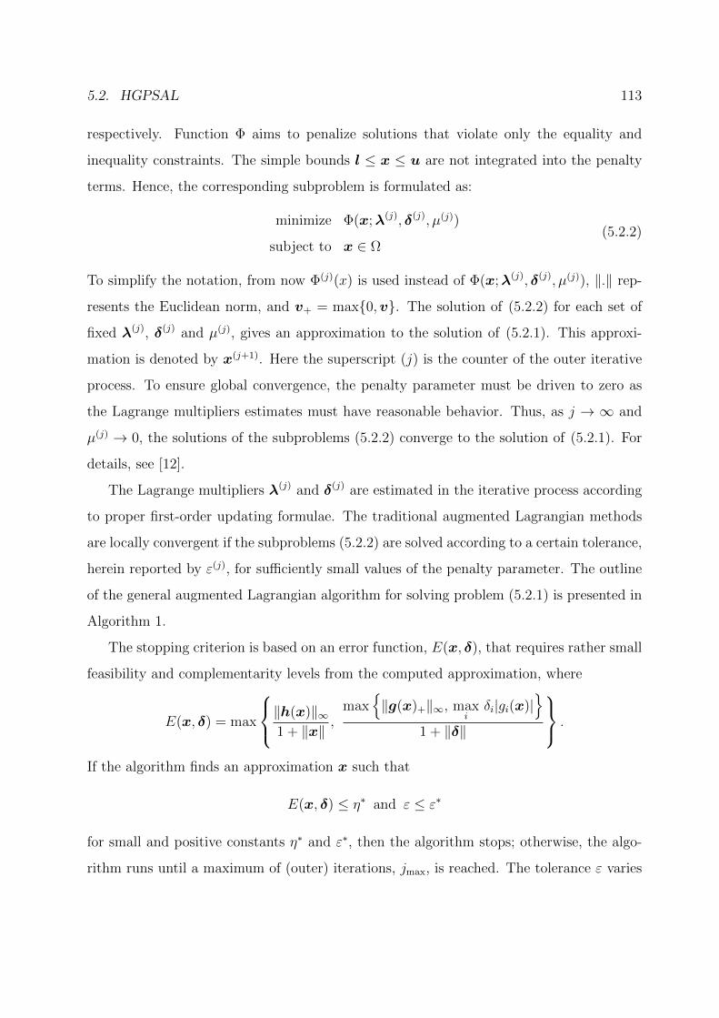
5.2. HGPSAL 113
respectively. Function Φ aims to penalize solutions that violate only the equality and
inequality constraints. The simple bounds l ≤ x ≤ u are not integrated into the penalty
terms. Hence, the corresponding subproblem is formulated as:
minimize Φ(x;λ(j), δ(j), µ(j))
subject to x ∈ Ω(5.2.2)
To simplify the notation, from now Φ(j)(x) is used instead of Φ(x;λ(j), δ(j), µ(j)), ‖.‖ rep-
resents the Euclidean norm, and v+ = max0,v. The solution of (5.2.2) for each set of
fixed λ(j), δ(j) and µ(j), gives an approximation to the solution of (5.2.1). This approxi-
mation is denoted by x(j+1). Here the superscript (j) is the counter of the outer iterative
process. To ensure global convergence, the penalty parameter must be driven to zero as
the Lagrange multipliers estimates must have reasonable behavior. Thus, as j → ∞ and
µ(j) → 0, the solutions of the subproblems (5.2.2) converge to the solution of (5.2.1). For
details, see [12].
The Lagrange multipliers λ(j) and δ(j) are estimated in the iterative process according
to proper first-order updating formulae. The traditional augmented Lagrangian methods
are locally convergent if the subproblems (5.2.2) are solved according to a certain tolerance,
herein reported by ε(j), for sufficiently small values of the penalty parameter. The outline
of the general augmented Lagrangian algorithm for solving problem (5.2.1) is presented in
Algorithm 1.
The stopping criterion is based on an error function, E(x, δ), that requires rather small
feasibility and complementarity levels from the computed approximation, where
E(x, δ) = max
‖h(x)‖∞1 + ‖x‖
,max
‖g(x)+‖∞, max
iδi|gi(x)|
1 + ‖δ‖
.
If the algorithm finds an approximation x such that
E(x, δ) ≤ η∗ and ε ≤ ε∗
for small and positive constants η∗ and ε∗, then the algorithm stops; otherwise, the algo-
rithm runs until a maximum of (outer) iterations, jmax, is reached. The tolerance ε varies

114 CHAPTER 5. HGPSAL
Algorithm 1 HGPSAL
1: input: λmin < λmax, δmax > 0, 0 < γ < 1, µmin 1, η∗ 1, ε∗ 1, λ(0)i ∈ [λmin, λmax],
i = 1, . . . , q, δ(0)i ∈ [0, δmax], i = 1, . . . , p, µ(0) > 0, η(0) > 0, π < 1;
2: Compute ε(0);
3: Randomly generate a point x(0) ∈ Ω;
4: j ← 0;
5: repeat
6: For a certain tolerance ε(j) find an approximate minimizer x(j+1) to
7: the subproblem (5.2.2) using Algorithm 2;
8: δ(j+1)i ← max
0,min
δ
(j)i + gi(x
(j+1))
µ(j) , δmax
, ∀i ∈ 1, . . . , p;
9: if E(x(j+1), δ(j+1)) ≤ η(j) then
10: λ(j+1)i ← λ
(j)i + max
λmin,min
hi(x
(j+1))
µ(j) , λmax
, ∀i ∈ 1, . . . , q;
11: µ(j+1) ← µ(j);
12: else
13: λ(j+1)i ← λ
(j)i ;
14: µ(j+1) ← maxµmin, γµ
(j)
;
15: end if
16: η(j+1) ← πη(j);
17: Compute ε(j+1);
18: j ← j + 1;
19: until the stopping criterion is met
20: output: xmin, fmin;
with the Lagrange multipliers and penalty parameter values according to
ε = τ(1 + ‖λ‖+ ‖δ‖+ (µ)−1
)−1, τ > 0.
Note that a decreasing sequence of µ values will yield a decreasing sequence of ε val-
ues forcing more and more accurate solutions to the subproblems (5.2.2). As shown in
Algorithm 1, the updating of the Lagrange multipliers relies on safeguards to maintain the
multiplier vectors bounded throughout the process. The sequence of penalty parameters
should also be maintained far away from zero so that solving the subproblem (5.2.2) is an

5.2. HGPSAL 115
Algorithm 2 GAPS
1: input x(j) ∈ Ω;
2: Y (j) ← GA(x(j));
3: X(j+1) ← HJ(Y (j));
4: x(j+1) ← compute the best point of X(j+1);
5: output: x(j+1) ∈ Ω;
easy task. The main differences between augmented Lagrangian algorithms are located on
the framework used to find an approximate global solution, for a defined tolerance ε(j), to
the subproblem (5.2.2). The herein proposed technique for solving (5.2.2) uses a popula-
tion based algorithm, known as genetic algorithm, followed by a local search procedure.
The outline of the hybrid genetic algorithm pattern search (GAPS) approach is shown in
Algorithm 2.
Since the genetic algorithm is a population based method, Y (j) is a set of y(j) points,
with best fitness found by the algorithm. Details concerning each step of the algorithm
are presented below.
5.2.2 Genetic Algorithm
In Algorithm 2, genetic algorithm is adopted with real representation of the search param-
eters to deal with continuous problems instead of the traditional binary representation.
The outline of GA is given by Algorithm 3.
GAs start from a population of points P of size s. Each point of the population
zl, for l = 1, . . . s, is an n dimensional vector. A fitness function is defined as evaluation
function in order to compare the points of the population and to apply a stochastic selection
that guarantees that better points are more likely to be selected. The fitness function
corresponds to the objective function of the subproblem (5.2.2), i.e., Φ(j)(x). A tournament
selection was considered, i.e., tournaments are played between two points and the best point
(with lower fitness value) is chosen for the mating pool.
New points in the search space are generated by the application of genetic operators
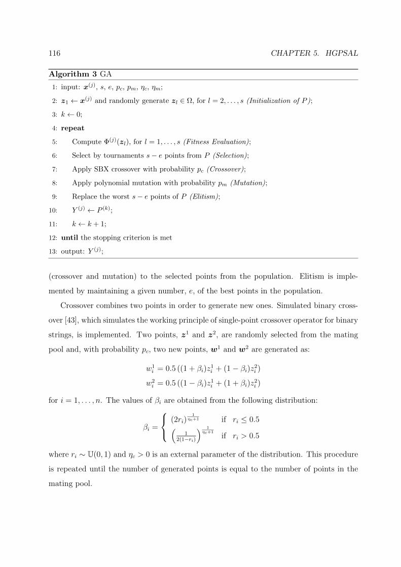
116 CHAPTER 5. HGPSAL
Algorithm 3 GA
1: input: x(j), s, e, pc, pm, ηc, ηm;
2: z1 ← x(j) and randomly generate zl ∈ Ω, for l = 2, . . . , s (Initialization of P );
3: k ← 0;
4: repeat
5: Compute Φ(j)(zl), for l = 1, . . . , s (Fitness Evaluation);
6: Select by tournaments s− e points from P (Selection);
7: Apply SBX crossover with probability pc (Crossover);
8: Apply polynomial mutation with probability pm (Mutation);
9: Replace the worst s− e points of P (Elitism);
10: Y (j) ← P (k);
11: k ← k + 1;
12: until the stopping criterion is met
13: output: Y (j);
(crossover and mutation) to the selected points from the population. Elitism is imple-
mented by maintaining a given number, e, of the best points in the population.
Crossover combines two points in order to generate new ones. Simulated binary cross-
over [43], which simulates the working principle of single-point crossover operator for binary
strings, is implemented. Two points, z1 and z2, are randomly selected from the mating
pool and, with probability pc, two new points, w1 and w2 are generated as:
w1i = 0.5 ((1 + βi)z
1i + (1− βi)z2
i )
w2i = 0.5 ((1− βi)z1
i + (1 + βi)z2i )
for i = 1, . . . , n. The values of βi are obtained from the following distribution:
βi =
(2ri)1
ηc+1 if ri ≤ 0.5(1
2(1−ri)
) 1ηc+1
if ri > 0.5
where ri ∼ U(0, 1) and ηc > 0 is an external parameter of the distribution. This procedure
is repeated until the number of generated points is equal to the number of points in the
mating pool.

5.2. HGPSAL 117
Since crossover cannot exclusively assure the exploration of new regions of the search
space, polynomial mutation is applied with a probability pm to the points produced by the
crossover operator. This operator guarantees that the probability of creating a new point
tl closer to the previous one wl (l = 1, . . . , s) is more than the probability of creating one
away from it. It can be expressed by:
tli = wli + (ui − li)ιi
for i = 1, . . . , n. The values of ιi are given by:
ιi =
(2ri)1
ηm+1 − 1 if ri < 0.5
1− (2(1− ri))1
ηm+1 if ri ≥ 0.5
where ri ∼ U(0, 1) and ηm > 0 is an external parameter of the distribution.
This procedure ends when |Φ(j)(z(k)best) − Φ(j)(z
(k−k∆)best )| ≤ εj, where Φ(j)(z
(k)best) is the
fitness value of the best point in the population, at iteration k, and k∆ is a parameter
that defines a periodicity for testing the criterion. However, if the stopping criterion is not
met in kmax iterations, the procedure is terminated and the best point in the population
is returned.
5.2.3 Hooke and Jeeves
A pattern search method is a derivative-free method that performs, at each iteration k, a
series of exploratory moves around a current approximation, z(k), in order to find a new
approximation z(k+1) = z(k)+∆(k)s(k), with a lower fitness value. In the following, k is used
for the iteration counter of this inner iterative process. For k = 0, the initial approximation
to start the search is z(0) = y(j) (y(j) ∈ Y (j)), see Algorithm 2. The scalar ∆(k) represents
the step length and the vector s(k) determines the direction of the step. The exploratory
moves to produce ∆(k)s(k), the updating of ∆(k) and s(k) defines a particular pattern search
method. Their choices are crucial to the success of the algorithm. If Φ(j)(zk+1) < Φ(j)(z(k))
then the iteration is considered successful; otherwise it is unsuccessful. If an iteration is

118 CHAPTER 5. HGPSAL
successful, the step length is not modified, while in an unsuccessful iteration ∆(k) is reduced.
For details, see [121, 175].
In the proposed approach, ∆(k)s(k) is computed by the Hooke and Jeeves (HJ) search
method [86]. This algorithm differs from the traditional coordinate search since it performs
two types of moves: the exploratory move and the pattern move. An exploratory move is a
coordinate search - a search along the coordinate axes - around a selected approximation,
using a step length of ∆(k). A pattern move is a promising direction that is defined by
z(k) − z(k−1) when the previous iteration was successful and z(k) was accepted as the new
approximation. A new trial approximation is then defined as z(k) + (z(k) − z(k−1)) and an
exploratory move is then carried out around this trial point. If this search is successful,
the new approximation is accepted as z(k+1). For details, see [86, 121]. This HJ iterative
procedure terminates providing a new set of approximations X(j+1) to the problem (5.2.1),
x(j+1) ← z(k+1), when the stopping condition is met, ∆(k) ≤ ε(j). However, if this condition
cannot be satisfied in kmax iterations, then the procedure is stopped with the last available
approximation.
The inner iterative process must return a feasible approximation. While using the
genetic algorithm and the Hooke and Jeeves method, any computed approximation x
that does not lie in the feasible set Ω is projected component by component as follows:
∀i ∈ 1, . . . , n : xi = minmaxxi, li, ui.
5.2.4 Performance Assessment
HGPSAL is implemented in the MATLAB R© programming language and tested on a set
of 24 benchmark problems. This set of difficult constrained problems with very distinct
properties is taken from [125]. The characteristics of these problems are summarized in
Table 5.1 that indicates the type of objective function, the number of decision variables
(n), the number of inequality constraints (p), the number of equality constraints (q), the
number of active constraints at the optimum (nact) and the optimal value known (fglobal).
All parameters of the HGPSAL algorithm are kept constant for all problems. No effort

5.2. HGPSAL 119
Prob. Type of f(x) n p q nact fglobal
g01 min quadratic 13 9 0 6 -15.00000
g02 max nonlinear 20 2 0 1 0.803619
g03 max polynomial 10 0 1 1 1.000000
g04 min quadratic 5 6 0 2 -30665.54
g05 min cubic 4 2 3 3 5126.498
g06 min cubic 2 2 0 2 -6961.814
g07 min quadratic 10 8 0 6 24.30621
g08 max nonlinear 2 2 0 0 0.095825
g09 min polynomial 7 4 0 2 680.6301
g10 min linear 8 6 0 6 7049.248
g11 min quadratic 2 0 1 1 0.750000
g12 max quadratic 3 1 0 0 1.000000
g13 min nonlinear 5 0 3 3 0.053945
g14 min nonlinear 10 0 3 3 -47.76488
g15 max quadratic 3 0 2 2 -961.7150
g16 min nonlinear 5 38 0 4 -1.905155
g17 min nonlinear 6 0 4 4 8853.539
g18 max quadratic 9 13 0 6 0.866025
g19 min nonlinear 15 5 0 0 32.65559
g20 min linear 24 6 14 16 0.204979
g21 min linear 7 1 5 6 193.7245
g22 min linear 22 1 19 19 236.4309
g23 min linear 9 2 4 6 -400.0551
g24 max linear 2 2 0 2 5.508013
Table 5.1: Test problems.

120 CHAPTER 5. HGPSAL
λmin λmax δmax µ0 µmin γ ε∗ η∗ λ0i ,∀i δ0i ,∀i η0 jmax
−1012 1012 1012 1 10−12 0.5 10−12 10−6 1 1 1 300
Table 5.2: Augmented Lagrangian parameters.
kmax s e pc ηc pm ηm ε ∆g
200 20 2 0.9 20 1/n 20 10−8 2n
Table 5.3: Genetic algorithm parameters.
is made in finding the best parameter setting for each problem. Table 5.2 shows the
parameters of the augmented Lagrangian used in all experiments. The genetic algorithm
parameters are listed in Table 5.3. The maximum number of function evaluations for
HGPSAL is set to 200, 000.
Hybridization Schemes
Four different hybridization schemes are proposed. They differ in the number of points of
the population that are selected to be improved in the local search. The tested alternatives
are: just one point, the best point of the population; the 10% best points; the 25% best
points; and the 50% best points. For simplicity, the hybridization schemes are denoted as
follows:
• version 1 that improves the best population point found by GA with HJ;
• version 2 that improves the best 10% population points found by GA with HJ;
• version 3 that improves the best 25% population points found by GA with HJ;
• version 4 that improves the best 50% population points found by GA with HJ.
Figure 5.1 allows to analyze the effect of the population size s on the algorithm perfor-
mance. The profiles in Figure 5.1(a), based on the metric favg, the central tendency of the
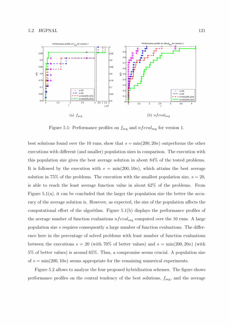
5.2. HGPSAL 121
1 1.5 2 2.5 30.6
0.65
0.7
0.75
0.8
0.85
0.9
0.95
1Performance profile on favg for version 1
τ
ρ(τ)
s=20s=40s=min(200,10n)s=min(200,20n)
0.5 1 1.5 2
x 104
0.6
0.65
0.7
0.75
0.8
0.85
0.9
0.95
1
(a) favg
1 1.5 2 2.5 3 3.5 40
0.1
0.2
0.3
0.4
0.5
0.6
0.7
0.8
0.9
1Performance profile on nfevalavg for version 1
τ
ρ(τ)
s=20s=40s=min(200,10n)s=min(200,20n)
(b) nfevalavg
Figure 5.1: Performance profiles on favg and nfevalavg for version 1.
best solutions found over the 10 runs, show that s = min(200, 20n) outperforms the other
executions with different (and smaller) population sizes in comparison. The execution with
this population size gives the best average solution in about 84% of the tested problems.
It is followed by the execution with s = min(200, 10n), which attains the best average
solution in 75% of the problems. The execution with the smallest population size, s = 20,
is able to reach the least average function value in about 62% of the problems. From
Figure 5.1(a), it can be concluded that the larger the population size the better the accu-
racy of the average solution is. However, as expected, the size of the population affects the
computational effort of the algorithm. Figure 5.1(b) displays the performance profiles of
the average number of function evaluations nfevalavg computed over the 10 runs. A large
population size s requires consequently a large number of function evaluations. The differ-
ence here in the percentage of solved problems with least number of function evaluations
between the executions s = 20 (with 70% of better values) and s = min(200, 20n) (with
5% of better values) is around 65%. Thus, a compromise seems crucial. A population size
of s = min(200, 10n) seems appropriate for the remaining numerical experiments.
Figure 5.2 allows to analyze the four proposed hybridization schemes. The figure shows
performance profiles on the central tendency of the best solutions, favg, and the average

122 CHAPTER 5. HGPSAL
1 1.2 1.4 1.6 1.8 20.4
0.5
0.6
0.7
0.8
0.9
1Performance profile on favg for s= min(200, 10 n)
τ
ρ(τ)
5000 100000.4
0.5
0.6
0.7
0.8
0.9
1
version 1version 2version 3version 4
(a) favg
1 1.2 1.4 1.6 1.8 20.3
0.4
0.5
0.6
0.7
0.8
0.9
1Performance profile on nfevalavg for s = min(200,10 n)
τ
ρ(τ)
version 1version 2version 3version 4
2 40.3
0.4
0.5
0.6
0.7
0.8
0.9
1
τ
(b) nfevalavg
Figure 5.2: Performance profiles on favg and nfevalavg for s = min(200, 10n).
number of function evaluations, nfevalavg, over 10 runs.
In Figure 5.2(a), it can observed that version 3 outperforms the other versions, attaining
the best average solution in more than 90% of the problems. Recall that this version
improves the best 25% best points of the population obtained by the GA algorithm with
the HJ local search. The worst performance is obtained by version 4, meaning that it is
self defeating to use an excessive number of points of the population to improve by local
search. As to the nfevalavg (Figure 5.2(b)), version 3 obtains the lower number of average
function evaluations in about 33% of the problems. Despite version 2 and version 4 are less
expensive in this item (42% of efficiency), it seems a good compromise to choose version 3
as the one that gives the best results.
Figure 5.3 shows the boxplot representations of the comparative performance of the
HGPSAL versions with different population sizes for the problem g02. It should be noted
that this problem is difficult and, in general, solvers fail to achieve an accurate approxima-
tion to the global optimum. The figure indicates the distribution of the approximations
obtained in 10 runs (the worst, upper quartile, median, lower quartile, and best approx-
imations are depicted). In Figures 5.3(a) and 5.3(b), it can be observed that the best
performance is obtained with the version 4, which presents the best median. However, for
larger population sizes, version 3 outperforms version 4 (Figures 5.3(c) and 5.3(d)).

5.2. HGPSAL 123
Version 1 Version 2 Version 3 Version 4
−0.8
−0.7
−0.6
−0.5
−0.4
−0.3
f(x)
s=20
(a) population size of 20.
Version 1 Version 2 Version 3 Version 4−0.8
−0.7
−0.6
−0.5
−0.4
−0.3
s=40
f(x)
(b) population size of 40.
Version 1 Version 2 Version 3 Version 4−0.8
−0.7
−0.6
−0.5
−0.4
−0.3
s=min(200,10n)
f(x)
(c) population size of min(200, 10n).
Version 1 Version 2 Version 3 Version 4
−0.8
−0.7
−0.6
−0.5
−0.4
−0.3
s=min(200,20n)f(
x)
(d) population size of min(200, 20n).
Figure 5.3: Boxplots for different population sizes (problem g02).
Performance Comparison
In order to compare the performance of HGPSAL with non-hybrid approaches using aug-
mented Lagrangian technique, two different algorithms are considered to find a minimizer
x(j+1) in Algorithm 1 (line 6). The first algorithm uses GA to find a solution for the sub-
problem (5.2.2), it is referred as GAAL. The second algorithm uses HJ to find a solution
for the subproblem (5.2.2), it is referred as HJAL. For each algorithm, 10 independent runs
are performed setting the maximum number of function evaluations equal to 200, 000. A

124 CHAPTER 5. HGPSAL
1 1.2 1.4 1.6 1.80
0.1
0.2
0.3
0.4
0.5
0.6
0.7
0.8
0.9
1
τ
ρ(τ)
1150515 525
HGPSALGAAL
HJAL
(a) fbest
1 2 3 4 5 60
0.1
0.2
0.3
0.4
0.5
0.6
0.7
0.8
0.9
1
τ
ρ(τ)
500 1500
HGPSALGAAL
HJAL
(b) fmedian
Figure 5.4: Performance profiles on fbest and fmedian.
population size of s = min(200, 20n) is used for HGPSAL and GAAL. For HJAL, the initial
solution is randomly generated within the bounds. Furthermore, version 2 of hybridiza-
tion is used for HGPSAL. The remaining parameter settings for Lagrangian and GA are
presented in Tables 5.2 and 5.3, respectively.
Figure 5.4 presents performance profiles on the best and the median function values
obtained over 10 runs. From Figure 5.4(a), it can be seen that HGPSAL outperforms other
algorithms in terms of accuracy achieving the best function values in 58% of the problems.
The second best is GAAL providing the best values in 38% of the problems. In terms of
robustness, the best algorithms is also HGPSAL followed by GAAL.
Figure 5.4(b) shows performance profile on the median function values. In terms of
accuracy, the best algorithm is HGPSAL, which provides the best median values in 67%
of the problems, followed by GAAL, which achieves the best median values in 25% of the
problems. In terms of robustness, the best algorithms is HGPSAL followed by HJAL.
From the above discussion, it can be concluded that the proposed hybridization of GA
and HJ with the augmented Lagrangian technique performs better than any of the consid-
ered algorithms separately. Thus, HGPSAL seems to be a valid optimizer for constrained
single-objective optimization.

5.3. MO-HGPSAL 125
5.3 MO-HGPSAL
So far in this chapter the optimization of single-objective function has been discussed. The
proposed HGPSAL shows ability to solve challenging constrained single-objective problems.
However, the focus of the present thesis is on solving multiobjective optimization problems.
Therefore, in the following the application of HGPSAL to multiobjective optimization is
discussed.
Chapter 3 discusses some classical methods for multiobjective optimization. Almost
all of them convert a given MOP into several SOPs. In particular, the normal boundary
intersection method and the normal constraint method transform unconstrained problems
into constrained ones. Such methods require to use efficient single-objective optimization
algorithms able to handle all types of constraints. In turn, as it is shown early in this chap-
ter, the proposed HGPSAL is an efficient algorithm for solving constrained optimization
problems. Thus, it seems a promising idea to apply HGPSAL to solve multiobjective op-
timization problems using scalarizing methods, which require to solve a set of constrained
single-objective optimization problems.
In the following, two approaches are considered to extend HGPSAL to solve MOPs.
First approach uses the normal boundary intersection method to perform scalarization, it
is referred as MO-HGPSALNBI. Second approach uses the normal constraint method to
perform scalarization, it is referred as MO-HGPSALNC. The outline of a general approach
to multiobjective optimization using HGPSAL (MO-HGPSAL) is shown in Algorithm 4.
Since both the NBI and NC methods require a knowledge of anchor (critical) points
needed to construct a hyperplane Φβ, the optimization process starts by initializing Φ =
(f(x1∗),f(x2∗), . . . ,f(xm∗)) and generating a set of evenly distributed points β ∈ B,
where ∀i ∈ 1, . . . ,m : 0 ≤ βi ≤ 1 ∧∑m
i=1 βi = 1. After that, ∀i ∈ 1, . . . , |B| : βi ∈ B,
the corresponding subproblem is solved using HGPSAL (line 4). A solution found after
solving each subproblem becomes an initial point for solving subsequent subproblem using
HGPSAL (line 5). All found solutions are stored in the archive A (line 6), which is
eventually returned as an approximation to the Pareto set for a given MOP.

126 CHAPTER 5. HGPSAL
Algorithm 4 MO-HGPSAL
1: initialize: x(0), β ∈ B, Φ = (f(x1∗), . . . ,f(xm∗));
2: A← ;
3: for β ∈ B do
4: (x∗,f(x∗))← HGPSAL(x(0)) on fagr;
5: x(0) ← x∗ ;
6: A← A ∪ x∗;
7: end for
8: output: A;
5.3.1 Performance Assessment
In the following, the performance of MO-HGPSALNBI and MO-HGPSALNC is studied
on the continuous ZDT test suite. All problems are adopted with 30 decision variables.
For each algorithm, 10 independent runs are performed on each problem, running for
100,000 function evaluations. The number of evenly distributed points used to construct
the hyperplane is 100 (B = β1, . . . ,β100). This means that 100 constrained single-
objective optimizations must be solved using HGPSAL.
Parameter settings adopted for HGPSAL are as follows. The version 1 of hybridization
is used. The maximum number of function evaluations for HGPSAL is set to 1,000. GA is
run for 10 generations with a population of 5 individuals. In this case, GA performs like
a micro-genetic algorithm. The maximum number of function evaluations used by Hooke
and Jeeves method is 50. The remaining parameter settings for HGPSAL are the same as
shown in Tables 5.2 and 5.3.
Table 5.4 presents the median values of IGD for the Pareto set approximations obtained
by MO-HGPSALNBI and MO-HGPSALNC after 10 runs. The best values are marked bold.
The last column in the table indicates the results of the Wilcoxon rank-sum test performed
at the significance level of α = 0.05, where “+” indicates that there is a significant difference
between two algorithms while “−” indicates that there is no significant difference between
two algorithms.

5.3. MO-HGPSAL 127
MO-HGPSALNBI MO-HGPSALNC significance
ZDT1 0.0375 0.0095 +
ZDT2 0.0138 0.0249 +
ZDT3 0.0388 0.0522 +
ZDT4 0.0879 0.0107 +
ZDT6 0.2394 0.2393 −
Table 5.4: Median values of IGD.
The results presented in Table 5.4 show that MO-HGPSALNBI performs better on
the ZDT2,3 test problems, whereas MO-HGPSALNC performs better on the ZDT1,4 test
problems. Additionally, MO-HGPSALNC provides the lower median value of IGD on ZDT6,
however, no significant difference is observed between the two algorithms on this problem.
Figure 5.5 depicts performance profiles on the best and median values of IGD. Analyzing
the presented plots, it can be concluded that both algorithms have quite similar perfor-
mance in terms of accuracy based on the best and median values of IGD. However, in terms
of robustness, MO-HGPSALNC outperforms MO-HGPSALNBI based on both best and me-
dian values of IGD. The better performance of MO-HGPSALNC in terms of robustness can
0 1 2 3 4 5 6 7 8 90
0.1
0.2
0.3
0.4
0.5
0.6
0.7
0.8
0.9
1
τ
ρ(τ)
MO−HGPSALNBI
MO−HGPSALNC
0 1 2 3 4 5 6 7 8 90
0.1
0.2
0.3
0.4
0.5
0.6
0.7
0.8
0.9
1
τ
ρ(τ)
MO−HGPSALNBI
MO−HGPSALNC
Figure 5.5: Performance profiles on the best (left hand side) and median (right hand side)
values of IGD.
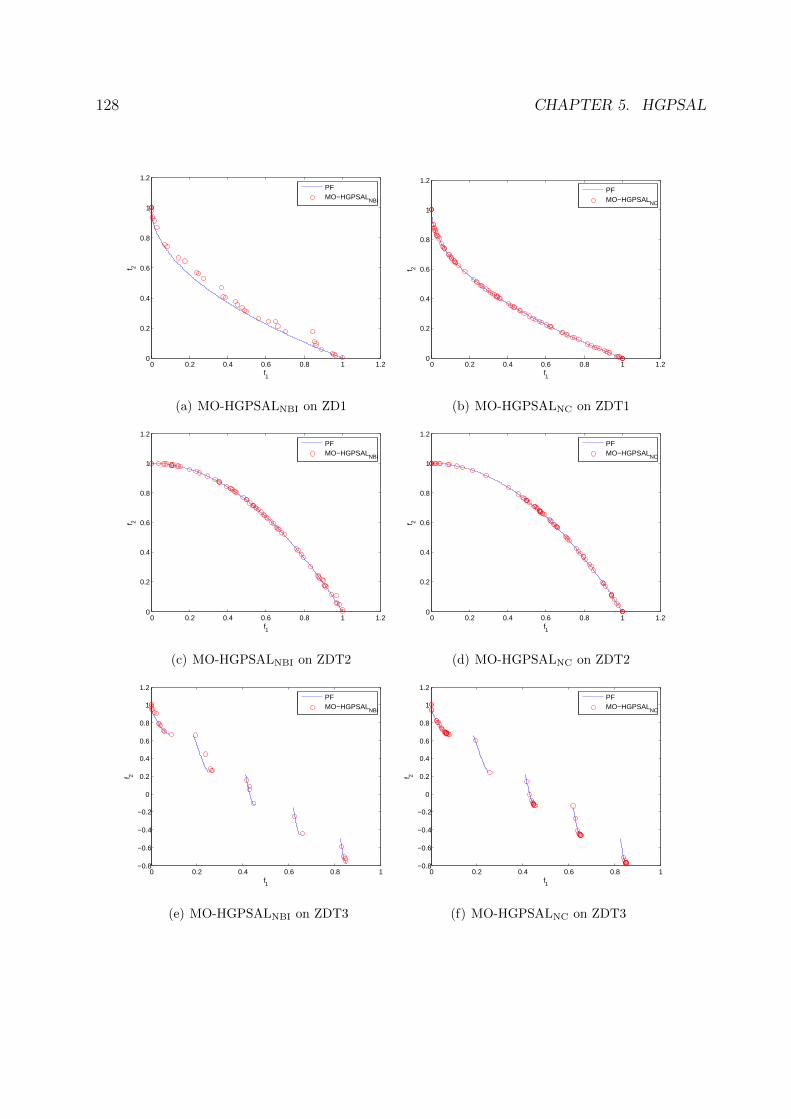
128 CHAPTER 5. HGPSAL
0 0.2 0.4 0.6 0.8 1 1.20
0.2
0.4
0.6
0.8
1
1.2
f1
f 2
PFMO−HGPSALNBI
(a) MO-HGPSALNBI on ZD1
0 0.2 0.4 0.6 0.8 1 1.20
0.2
0.4
0.6
0.8
1
1.2
f1
f 2
PFMO−HGPSALNC
(b) MO-HGPSALNC on ZDT1
0 0.2 0.4 0.6 0.8 1 1.20
0.2
0.4
0.6
0.8
1
1.2
f1
f 2
PFMO−HGPSALNBI
(c) MO-HGPSALNBI on ZDT2
0 0.2 0.4 0.6 0.8 1 1.20
0.2
0.4
0.6
0.8
1
1.2
f1
f 2
PFMO−HGPSALNC
(d) MO-HGPSALNC on ZDT2
0 0.2 0.4 0.6 0.8 1−0.8
−0.6
−0.4
−0.2
0
0.2
0.4
0.6
0.8
1
1.2
f1
f 2
PFMO−HGPSALNBI
(e) MO-HGPSALNBI on ZDT3
0 0.2 0.4 0.6 0.8 1−0.8
−0.6
−0.4
−0.2
0
0.2
0.4
0.6
0.8
1
1.2
f1
f 2
PFMO−HGPSALNC
(f) MO-HGPSALNC on ZDT3

5.3. MO-HGPSAL 129
0 0.2 0.4 0.6 0.8 1 1.20
0.2
0.4
0.6
0.8
1
1.2
f1
f 2
PFMO−HGPSALNBI
(g) MO-HGPSALNBI on ZD4
0 0.2 0.4 0.6 0.8 1 1.20
0.2
0.4
0.6
0.8
1
1.2
f1
f 2
PFMO−HGPSALNC
(h) MO-HGPSALNC on ZDT4
0.2 0.4 0.6 0.8 1 1.20
0.2
0.4
0.6
0.8
1
1.2
f1
f 2
PFMO−HGPSALNBI
(i) MO-HGPSALNBI on ZDT6
0.2 0.4 0.6 0.8 1 1.20
0.2
0.4
0.6
0.8
1
1.2
f1
f 2
PFMO−HGPSALNC
(j) MO-HGPSALNC on ZDT6
Figure 5.6: Performance of MO-HGPSAL on the ZDT test suite.
be explained by the fact that it seems to be easier for HGPSAL to solve a constrained
problem with inequality rather than equality constraints. Therefore, MO-HGPSALNC can
be considered a good choice to handle multiobjective optimization problems. However,
the major limitations of this approach is a high computational cost and the need to pro-
vide the critical points of the Pareto front in advance. Since some studies have clearly
shown that EMO algorithms are more efficient for solving MOPs than classical methods
for multiobjective optimization [161, 181], the performance comparison of MO-HGPSAL
with multiobjective evolutionary algorithms is not provided in this chapter. Additionally,
the Pareto front approximations with the lowest values of IGD obtained by both algorithms
over 10 runs are presented in Figure 5.6.

130 CHAPTER 5. HGPSAL
5.4 Summary
Many optimization problems in science and engineering involve a number of constraints,
which the optimal solution must satisfy. Such problems are posed as constrained opti-
mization problems. There are many studies on solving constrained optimization problems.
Penalty function methods are among the most popular approaches, because of their simplic-
ity and ease of implementation. In general, the penalty function approaches are applicable
to any type of constraints (inequality or equality).
This chapter introduces a new hybrid algorithm within an augmented Lagrangian
framework for constrained optimization. In each iteration of the augmented Lagrangian, a
set of promising solutions is found by a genetic algorithm. Afterwards, a specified number
of these solutions is improved using a pattern search method. It is shown that the hybrid
approach exhibits a better performance than each of the methods separately. Moreover,
different hybridization schemes are investigated.
The proposed single-objective algorithm is extended to solve MOPs. Two variants of the
resulting multiobjective approach are developed. The first variant uses the NBI method for
converting MOP into SOP. The second variant employees the NC method for scalarization.
The performance of both variants is studied on the continuous ZDT test suite. Although
two variants show ability to solve MOPs producing quite similar performance in terms
of IGD, there are some disadvantages of MO-HGPSAL compared with EMO algorithms.
Since both variants use a hyperplane passing through the critical points of the Pareto
front, these points must be known before the search. One way to overcome this limitation
is to apply a single-objective optimizer to find a minimum of each objective. However,
this does not guarantee that the obtained points will be critical. On the other hand, MO-
HGPSAL needs to perform a relatively large number of function evaluations. This may
be unacceptable to solve real-world optimization problems with computationally expensive
function evaluations. Therefore, the following chapters address MO using EAs designed to
overcome these limitations.

Chapter 6
Descent Directions-Guided
Multiobjective Algorithm
6.1 Introduction
This chapter introduces a descent directions-guided multiobjective algorithm (DDMOA).
DDMOA is a hybrid multiobjective evolutionary algorithm, which borrows the idea of
generating new promising solutions from Timmel’s method incorporating it in a general
framework of EMO algorithms. In order to overcome the limitations of original Timmel’s
method imposed by the assumptions of differentiability of the objective functions, descent
directions for each objective are used instead of the gradients. Thus, new promising solu-
tions are generated by adding to a parent solution a linear combination of descent directions
for each objective function. In DDMOA, these descent directions are calculated using a
pattern search method. However, it is clear that performing computation of descent di-
rections for each population member and for each objective function is an inefficient way
to conduct the search. Therefore, a strategy based on subpopulations is implemented to
avoid the direct computation of descent directions for the entire population. This sim-
ple mechanism is proposed to avoid computational overhead caused by the local search
procedure.
131

132 CHAPTER 6. DDMOA
6.2 DDMOA
The main loop of DDMOA is given by Algorithm 5. It is a hybrid evolutionary algorithm
with (µ+λ) selection scheme, where in each generation the adaptation of strategy param-
eters of population members is followed by the successive application of parent selection,
mutation, and environmental selection.
In DDMOA, the population consists only of nondominated individuals. Furthermore,
an individual ai in the current population P (g) in generation g is a tuple of the form
[xi, δi,Si, σi], where xi ∈ Rn is the decision vector, δi > 0 is the step size used for local
search, Si ∈ Rn×m is the search matrix, and σi > 0 is the step size used for reproduction.
DDMOA starts by randomly generating an initial population P 0 of size µ and initial-
izing the set of strategy parameters of each population member. Then, the population is
evaluated and all dominated individuals are removed from the population. The evolution-
ary process is started by computing descent directions for each objective for all individuals
in the population in updateSearchMatrix procedure. These directions are stored in the
search matrix S of the corresponding individual. Additionally, during this procedure all
nondominated solutions with respect to the current population found during local search
Algorithm 5 DDMOA
1: g ← 0;
2: initialize: P (g);
3: repeat
4: g ← g + 1;
5: (P (g), Q(g))← updateSearchMatrix(P (g));
6: P (g) ← updateStepSize(P (g));
7: R(g) ← parentSelection(P (g));
8: Q(g) ← mutation(R(g), Q(g));
9: P (g) ← environmentalSelection(P (g) ∪Q(g));
10: until the stopping criterion is met
11: output: P (g);

6.2. DDMOA 133
are added to the offspring population, which is empty at the beginning of each generation.
Next, the step size σ of each individual a is updated in updateStepSize procedure. Then,
in order to select a pool of parents R(g), parentSelection procedure is performed that
uses binary tournament selection based on crowding distance. After the pool of parents is
selected, a set of offspring is generated and added to the offspring population in mutation
procedure. Then, a set of fittest individuals is selected from the composed multiset in
environmentalSelection procedure. This procedure selects nondominated individuals
and uses crowding distance to keep the population of bounded size. Finally, if the stopping
criterion is met, the evolutionary process terminates, and the algorithm returns its final
population, otherwise the algorithm proceeds to the next generation. The following two
stopping conditions are used: (i) the maximum number of objective function evaluations
is reached, and (ii) δ ≤ δtol for all individuals in the population.
In the following, the components of DDMOA are discussed in more detail.
6.2.1 Initialize Procedure
First, the initial population is generated and the set of strategy parameters is initialized
P 0 = [x(0)i , δ
(0)i ,S
(0)i , σ
(0)i ], ∀i ∈ 1, . . . , µ. The initial values of decision vectors ∀i ∈
1, . . . , µ : x(0)i can be generated in multiple ways. They can be either generated randomly
such that all the variables are inside the search space or can be uniformly sampled. In turn,
DDMOA creates the initial population using Latin hypercube (LH) sampling [126] since it
gives a good overall random distribution of the population in the decision space. The set
of strategy parameters of each generated individual is initialized taking default values.
After the initial populations is sampled, it is evaluated and only nondominated indi-
viduals are retained while all dominated solutions are removed from the population. So
usually the number of individuals in P 0 is less than µ.

134 CHAPTER 6. DDMOA
6.2.2 Update Search Matrix Procedure
The procedure updateSearchMatrix is used to update the search matrix of each individual
in the current population. Each column of the search matrix stores a descent direction
for the corresponding objective function. Thus, to update the search matrix of a given
individual, m descent directions need to be computed. The procedure is designed in such a
way that the direct computation of descent directions for all individual is avoided, thereby
alleviating the computational burden.
Main Loop
The steps of updateSearchMatrix procedure are outlined in Algorithm 6.
Algorithm 6 updateSearchMatrix
1: input: P ;
2: Q← ;
3: for m = 1 . . .M do . M - is the number of objectives
4: i← 0;
5: sort population P in ascending order according to fm;
6: partition sorted P into α subpopulations:
7: P = p1, p2, .., pα;
8: for k = 1 . . . α do
9: identify the leader individual aleader ∈ pk;
10: (aleader, sleader, Q)← localSearch(aleader,m,Q);
11: for j = 1 . . . |pk| do
12: i← i+ 1;
13: Si( : ,m)← xleader − xi + sleader;
14: end for
15: end for
16: end for
17: output: P , Q;

6.2. DDMOA 135
The search matrices of all individuals in the current population are updated by columns.
At the beginning, the first column of the search matrix of each individual, which stores
a descent direction for the first objective, is updated. Then, the second column of the
search matrix of each individual, which stores a descent direction for the second objective,
is updated and so on.
For each objective function, the population is sorted in ascending order and partitioned
into α equal parts. This way, α subpopulations are defined in order to promote different
reference points for the computation of descent directions. It follows that in each sub-
population pk a leader individual aleader is selected. The leader of the subpopulation is a
solution with the lower value of the corresponding objective function among other solutions
in the subpopulation and δ > δtol. Thus, if δ ≤ δtol of the solution with the lower value
of the corresponding objective then the second best solution is selected as the leader and
so on. Thereafter, a descent direction for the m-th objective function is computed for the
leader in localSearch procedure (line 10). The procedure localSearch returns the leader
with updated set of the strategy parameters, descent direction for the leader, and offspring
population Q, which at the moment contains individuals nondominated with respect to
the current population found in localSearch procedure. Using descent direction sleader,
the m-th column of the search matrix of each individual in the subpopulation is updated:
Si( : ,m) = xleader − xi + sleader, (6.2.1)
where Si( : ,m) is the m-th column of the search matrix of the i-th individual in the
subpopulation, xi is the decision vector of the i-th individual in the subpopulation, xleader
is subpopulation leader, and sleader is descent direction for the leader. At the end, all
m columns of the search matrix S of each individual in the population are updated.
Partitioning the population into different subpopulations and the calculation of descent
directions for solutions in the subpopulation based on a descent direction for the leader
allow to significantly reduce the number of function evaluations. This way, the direct
computation of descent directions for the entire population using localSearch procedure,
which is computationally expensive, is avoided.

136 CHAPTER 6. DDMOA
1f
2f1s
1º subpopulation
2º subpopulation
3º subpopulation
1
2
3
4
6
7
8
9 1011
52s
3s
(a) descent directions for f1
1f
2f
1º subpopulation
2º subpopulation
3º subpopulation
1234
6
7
8
9
10
11
5
1s
2s
3s
(b) descent directions for f2
Figure 6.1: Representation of the working principle of updateSearchMatrix procedure in
the objective space.
The working principle of updateSearchMatrix procedure is illustrated in Figure 6.1.
The figure presents the population of 11 nondominated solutions at some generation of the
algorithm. The population and the corresponding directions are shown in the objective
space. Solid arrows denote descent directions found for subpopulation leaders while dashed
arrows denote descent directions for the remaining individuals.
In Figure 6.1(a), the population is sorted according to f1. Three subpopulations are
defined (α = 3). The first and second subpopulations consist of 4 individuals, whereas the
third subpopulation consists of 3 individuals. When the exact division is not possible, the
last subpopulation has always less individuals. In the first subpopulation, solution 1 is the
leader. Descent direction with respect to f1 for the leader is S1. Dashed arrows from points
2, 3, 4 show descent directions for the corresponding solutions in the first subpopulation.
In the second subpopulation, the leader is solution 5. Descent direction with respect to
f1 for the leader is S2. Dashed arrows from points 6, 7, 8 show descent directions for
the corresponding solutions in the second subpopulation. In the third subpopulation, the
leader is solution 9. Descent direction with respect to f1 for the leader is S3. Dashed

6.2. DDMOA 137
arrows from points 10, 11 show descent directions for the corresponding individuals in
the third subpopulation.
In Figure 6.1(b), the population is sorted according to f2. Three subpopulations are
defined. In the first subpopulation, solution 1 is the leader. Descent direction with respect
to f2 for the leader is S1. Dashed arrows from points 2, 3, 4 show descent directions for
the corresponding solutions in the first subpopulation. In the second subpopulation, the
leader is solution 6. Although solution with the lower value of f2 in the second subpopu-
lation is solution 5, solution 6 is chosen as leader because δ5 < δtol. This means that the
vicinity of this solution has been already explored. Consequently, the next best solution
is chosen. Thus, descent direction with respect to f2 for the leader is S2. Dashed arrows
from points 5, 7, 8 show descent directions for the corresponding solutions in the second
subpopulation. In the third subpopulation, the leader is solution 9. Descent direction
with respect to f2 for the leader is S3. Dashed arrows from points 10, 11 show descent
directions for the corresponding solutions in the third subpopulation.
Local Search Procedure
In line 10 of Algorithm 6, localSearch procedure is invoked to compute descent directions
for subpopulation leaders. In general, any local search procedure can be used for this
purpose. DDMOA uses a simple coordinate search method [175], which is adopted with
slight modifications. The steps of localSearch procedure are outlined in Algorithm 7.
A randomization procedure is introduced whose idea is similar to that used in facto-
rial design where the experiment is performed in a random order to guarantee that the
environment in which treatments are applied is as uniform as possible, and the unknown
biases are avoided. Thus, this procedure randomly generates the order of the variables to
be tested (line 3), instead of the usual standard order, and the direction along which a
given variable is tested (line 4). The order of the variables and the corresponding direction
are determined randomly so that the algorithm can escape from a local optimum during
the coordinate search. This becomes even more relevant to large-scale problems.

138 CHAPTER 6. DDMOA
Algorithm 7 localSearch
1: input: a = [x, δ,S, σ], m, Q;
2: s← 0, ρ← 0, min← fm(x);
3: order ← randomly permute 1, 2, . . . , n;
4: direction ← randomly permute 1,−1 ;
5: while δ > δtol do
6: for i = order do
7: for d = direction do
8: strial ← s+ d δ ei; . ei denotes the standard coordinate vector
9: xtrial ← x+ strial;
10: evaluate f(xtrial);
11: if @y ∈ P : y ≺ xtrial then
12: Q← Q ∪ xtrial;
13: end if
14: if fm(xtrial) < min then
15: ρ← min− fm(xtrial);
16: min← fm(xtrial);
17: s← strial;
18: break
19: end if
20: end for
21: end for
22: if ρ > 0 then
23: break
24: else
25: δ ← δ/2;
26: end if
27: end while
28: output: a = [x, δ,S, σ], s, Q;
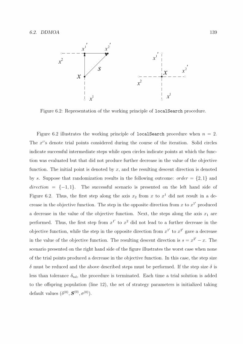
6.2. DDMOA 139
1x
2x
1x
2x
1x
2x
2x
1x
x xs
Figure 6.2: Representation of the working principle of localSearch procedure.
Figure 6.2 illustrates the working principle of localSearch procedure when n = 2.
The xi’s denote trial points considered during the course of the iteration. Solid circles
indicate successful intermediate steps while open circles indicate points at which the func-
tion was evaluated but that did not produce further decrease in the value of the objective
function. The initial point is denoted by x, and the resulting descent direction is denoted
by s. Suppose that randomization results in the following outcome: order = 2, 1 and
direction = −1, 1. The successful scenario is presented on the left hand side of
Figure 6.2. Thus, the first step along the axis x2 from x to x1 did not result in a de-
crease in the objective function. The step in the opposite direction from x to x1′ produced
a decrease in the value of the objective function. Next, the steps along the axis x1 are
performed. Thus, the first step from x1′ to x2 did not lead to a further decrease in the
objective function, while the step in the opposite direction from x1′ to x2′ gave a decrease
in the value of the objective function. The resulting descent direction is s = x2′ − x. The
scenario presented on the right hand side of the figure illustrates the worst case when none
of the trial points produced a decrease in the objective function. In this case, the step size
δ must be reduced and the above described steps must be performed. If the step size δ is
less than tolerance δtol, the procedure is terminated. Each time a trial solution is added
to the offspring population (line 12), the set of strategy parameters is initialized taking
default values (δ(0),S(0), σ(0)).

140 CHAPTER 6. DDMOA
Algorithm 8 updateStepSize
1: input: P ;
2: for i = 1, . . . , |P | do
3: σi = maxσ(0)
g , δtol
;
4: end for
5: output: P ;
6.2.3 Update Step Size Procedure
As it is mentioned earlier, step size σ is associated with each individual in the population.
The step size is used to control the mutation strength. In Algorithm 5, step size σ of each
individual is updated in updateStepSize procedure.
However, there is no common rule to update step size σ, but it must be done carefully
to ensure convergence to the Pareto optimal set. DDMOA uses a simple deterministic
parameter control rule, where values of σ are determined as a function of time (generation).
The outline of updateStepSize procedure is given by Algorithm 8.
Using this method step size σ is equal among individuals in the population and de-
creases during the generations from the initial value σ(0) at the first generation and never
becomes less then δtol. Graphically, step size adaptation during the generations is shown
in Figure 6.3.
g
0
tol
1
)(g
Figure 6.3: Step size adaptation.

6.2. DDMOA 141
6.2.4 Parent Selection Procedure
At every generation, a pool of parents R of size µ is selected in parentSelection procedure.
The outline of this procedure is shown in Algorithm 9. The procedure parentSelection
performs binary tournament selection based on crowding distance measured in the objec-
tive space. Therefore, individuals with the higher crowding distances have more probability
of creating offspring. However, as DDMOA uses only nondominated solutions, the situa-
tion where the number of individuals in the population is very small or even equal to one
may occur. So if the number of solutions in the population is less or equal to the number of
objectives then parents are randomly selected from given individuals. Otherwise tourna-
ment selection is performed. This selection process that combines crowding distance with
a stochastic selection operator promotes a good spread of solutions in the objective space
Algorithm 9 parentSelection
1: input: P ;
2: R← ;
3: while |R| < µ do
4: if |P | ≤M then
5: randomly pick a ∈ P ;
6: R← R ∪ a;
7: else
8: randomly pick a ∈ P , b ∈ P ∧ a 6= b;
9: if I[a] < I[b] then . I[] denotes crowding distance measure
10: R← R ∪ b;
11: else
12: R← R ∪ a;
13: end if
14: end if
15: end while
16: output: R;

142 CHAPTER 6. DDMOA
Algorithm 10 mutation
1: input: R = [xi, δi,Si, σi] : 1 ≤ i ≤ |R|, Q;
2: for i = 1, . . . , |R| do
3: x′i ← xi + σiSi ν;
4: x′i ← minmaxx′i, l,u;
5: evaluate x′i;
6: Q← Q ∪ x′i;
7: end for
8: output: Q;
as well as the exploration of new promising areas of the decision space.
6.2.5 Mutation Procedure
After the pool of parents is selected, offspring are generated by mutating the corresponding
parent in mutation procedure. The outline of this procedure is given by Algorithm 10.
Search matrix S and step size σ of the parent are used for the mutation (line 3), where ν
is a column vector of random numbers (∀i ∈ 1, . . . ,m : νi ∼ U(0, 1)). The mutation is
similar to that used in Timmel’s method. The only difference is that the gradients of the
objective functions are replaced by descent directions, which are stored in search matrix S.
In order to guarantee that each new solution x′ = [x′1, . . . , x′n]T belongs to Ω, projection
is applied to each component of the decision vector (line 4). After offspring x′ is repaired,
it is evaluated (line 5) and added to the offspring population (line 6), which is initialized
in localSearch procedure by saving promising solutions found during the computation of
descent directions.
6.2.6 Environmental Selection Procedure
The procedure environmentalSelection is used to select a set of fittest individuals from
the multiset composed of parents and offspring. The outline of environmentalSelection
procedure is shown in Algorithm 11. Two main steps of environmentalSelection proce-

6.3. PERFORMANCE ASSESSMENT 143
Algorithm 11 environmentalSelection
1: input: P ′ = P ∪Q;
2: P ← ;
3: for i = 1, . . . , |P ′| do
4: for j = 1, . . . , |P ′| and j 6= i do
5: if P ′(j) ≺ P ′(i) then
6: break
7: end if
8: end for
9: if j = |P ′| then
10: P ← P ∪ P ′(i);
11: end if
12: end for
13: if |P | > µ then
14: P ← truncation(P );
15: end if
16: output: P ;
dure can be distinguished. First, all dominated individuals are removed from the combined
population (lines 3-12). Then, if the size of the resulting population P is greater than user-
specified population size µ, truncation procedure (lines 14) is used to reduce the number
of individuals in the population, at the same time, preserving diversity among popula-
tion members. DDMOA uses truncation procedure based on crowding distance, where
individuals having higher values of crowding distance measure are selected for the next
generation.
6.3 Performance Assessment
This section presents and discusses empirical results obtained by DDMOA. The perfor-
mance produced by DDMOA is compared with that produced by representative state-of-

144 CHAPTER 6. DDMOA
the-art multiobjective evolutionary algorithms. The experimental study is performed in
two stages. In the first stage, the performance of original DDMOA is studied. In the
second stage, more extensive study is performed, where DDMOA is tested with slight
modifications.
6.3.1 Preliminary Experiments
In this study, the results obtained by DDMOA are compared with that produced by
NSGA–II [46], SPEA2 [200] and AbYSS [136]. The performance of all algorithms is stud-
ied on the ZDT [197] (except for ZDT5, which is a binary problem) and three-objective
DTLZ [50] test suites.
Experimental Setup
DDMOA is implemented in the MATLAB R© programming language, whereas the other
algorithms are used within the jMetal framework [62]. Problems ZDT1-3 and 6 are used
with 30 decision variables, and ZDT4 is tested using 10 decision variables. Problems
DTLZ1-6 are adopted with 12 decision variables, and DTLZ7 is tested with 22 decision
variables. For each algorithm, 30 independent runs are performed on each problem with
population size of µ = 100, running for 20, 000 function evaluations. Further, the size of
archive in SPEA2 and AbYSS is set to 100, while the default settings are used for the other
parameters. Parameter settings used in DDMOA are the following: the initial step size for
local search δ(0) = 1, the initial step size for reproduction σ(0) = 5, the tolerance for step
size δtol = 10−3, the number of subpopulations α = 5. Although DDMOA uses the step
size adaptation rule presented in Algorithm 8, in this study the step size is updated as:
σ = maxσ(0)(1− g/Eg), 1
,
where Eit = 10 is the expected number of generations, and g is the current generation.

6.3. PERFORMANCE ASSESSMENT 145
1 1.5 2 2.5 30
0.1
0.2
0.3
0.4
0.5
0.6
0.7
0.8
0.9
1
τ
ρ(τ)
69.5 80
DDMOANSGA2SPEA2AbYSS
(a) median values of Iε+
1 1.05 1.1 1.15 1.2 1.250
0.1
0.2
0.3
0.4
0.5
0.6
0.7
0.8
0.9
1
τ
ρ(τ)
45 123
DDMOANSGA2SPEA2AbYSS
(b) median values of I−H
Figure 6.4: Performance profiles on the median values of quality indicators.
Experimental Results
Figure 6.4 shows the median run comparisons in terms of the epsilon and hypervolume
indicators. Figure 6.4(a) shows that the most accurate algorithm with respect to the
epsilon indicator is DDMOA together with AbYSS, providing the best median values in
33% of the tested problems. In terms of robustness with respect to Iε+, the best algorithm
is DDMOA. Figure 6.4(b) shows that the most accurate algorithm with respect to the
hypervolume indicator is DDMOA, providing the best median values in 50% of the tested
problems. In terms of robustness with respect to I−H , the best algorithm is again DDMOA.
Large difference in the values of τ for ρ(1) observed in the above plots is explained by the
fact that NSGA2, SPEA2, and AbYSS face difficulties in finding adequate approximation
sets within the given number of function evaluations (20,000) on the DTLZ1 and DTLZ3
problems. This results in higher values of Iε+ and I−H . On the contrary, DDMOA obtains
good approximation sets on these problems. This result is achieved due to the reproduction
operator used in DDMOA. While the other three considered EMO algorithms use stochastic
reproduction operators that may often require a significant computational effort to be spent
until the optimal region is reached, DDMOA uses the combination of a pattern search
method to learn the fitness landscape and a stochastic technique to generate offspring.

146 CHAPTER 6. DDMOA
0
0.2
0.4
0.6
0.8
0
0.20.4
0.60.8
0
0.2
0.4
0.6
0.8
f1f2
f 3
PFDDMOA
(a) DTLZ1
0
0.5
1
1.5
0
0.5
1
1.5
0
0.5
1
1.5
f1f2
f 3
PFDDMOA
(b) DTLZ3
Figure 6.5: Performance of DDMOA on DTLZ1 and DTLZ3 using 10,000 evaluations.
This allows DDMOA to reach Pareto optimal region much faster than the other algorithms,
especially on multimodal functions.
To reinforce these observations and to show the ability and efficiency of DDMOA in
solving multimodal DTLZ1,3 problems, DDMOA is run on these two problems setting
only the half of function evaluations as stopping criterion (10,000). Figure 6.5 presents
approximation sets with the best values of the hypervolume indicator obtained by DDMOA
after 30 runs. From Figures 6.5(a) and 6.5(b), it can be seen that DDMOA is able to find
adequate approximations even within 10,000 function evaluations.
6.3.2 Intermediate Summary
In the performed experiments, DDMOA is tested on a set of problems and compared with
state-of-the-art EMO algorithms. The obtained results reveal that DDMOA is able to solve
a set of benchmark multiobjective problems. The proposed scheme to search for descent
directions using local search combined with the strategy based on subpopulations is able to
learn the fitness landscape and to generate new promising solutions spending a reasonable
computational effort. When compared with other multiobjective solvers, DDMOA provides
competitive results with respect to the epsilon and hypervolume indicators. Furthermore,

6.3. PERFORMANCE ASSESSMENT 147
the experimental results show that DDMOA outperforms the other considered algorithms
on multimodal problems due to its hybrid reproduction operator. Moreover, it is observed
that DDMOA is able to find adequate approximations at much lower computational cost.
6.3.3 Further Experiments
In this experimental study, the performance of DDMOA is further studied on a set of
challenging problems. DDMOA is compared to popular EMO algorithms, namely, NSGA–
II [46], IBEA [198] (in combination with the epsilon indicator), and MOEA/D [123].
Thus, DDMOA is compared against different algorithmic frameworks (dominance-based,
indicator-based, and decomposition-based) employing different reproduction operators (ge-
netic and DE operators). The performance of all algorithms is studied on the ZDT [197],
DTLZ [50], and WFG [88] test suites.
Experimental Setup
DDMOA is implemented in the MATLAB R© programming language, whereas the other
algorithms are used within the jMetal framework [62]. All two and three-objective DTLZ
and ZDT test problems except for ZDT4 are adopted with 30 decision variables, ZDT4
is tested using 10 decision variables. All two and three-objective WFG test problems are
tested with 10 decision variables (k = 4 position-related parameters and l = 6 distance-
related parameters). Additionally, WFG1 is used with a slight modification to the original
definition presented in [88].
For all algorithms, 30 independent runs are performed on each test problem. The
population size is set to 100 and the maximum number of function evaluations is set to
15,000 and 20,000 for the two-objective and three-objective test problems, respectively. All
other parameter settings for NSGA–II, IBEA, and MOEA/D are default as defined in [62].
The parameter settings for DDMOA are the following: the initial step size for local
search δ(0) = 1, the initial step size for reproduction σ(0) = 5, the tolerance for step size
δtol = 10−3, and the number of subpopulations α = 5. In order to focus on promising re-

148 CHAPTER 6. DDMOA
1f
2f
leaderx
leaderssubpopulation
trailx
(a) without additional condition
1f
2f
leaderxleaders
subpopulationtrailx
(b) with additional condition
Figure 6.6: Computation of descent directions for leaders.
gions of the search space, an additional condition for the acceptance of descent directions
calculated for subpopulation leaders in localSearch procedure is introduced. Thus, de-
scent direction s is accepted for subpopulation leader xleader if two conditions are satisfied:
(i) if s leads to a decrease in the value of the corresponding objective, and (ii) if a trail
solution xtrail = xleader + s is nondominated with respect to the current population (i.e.
when a trail is added to the offspring population). To better understand this idea consider
Figure 6.6, which presents a set of nondominated solutions in the objective space. Suppose
that a descent direction needs to be computed with respect to f1 for subpopulation leader
xleader.
Figure 6.6(a) shows a possible descent direction sleader that leads to the decrease in
the value of f1. It can be see that xtrail is dominated with respect to the population, so
the descent direction shown in this figure may not lead to a promising region. On the
other hand, Figure 6.6(b) shows a descent direction that can be obtained by introducing
the condition that xtrail should be nondominated with respect to the population. This
way, the possibility of obtaining a descent direction shown in Figure 6.6(a) is excluded,
consequently the search pressure is increased. Thus, the DDMOA framework provides
an additional feature to guide the search that can be easily exploited depending on the

6.3. PERFORMANCE ASSESSMENT 149
characteristics of a given problem.
Furthermore, from Figure 6.5, one can see that DDMOA is able to converge to the
Pareto front at low computational cost. However, the overall distribution of solutions along
the Pareto front is not so good. Thus, to obtain a well-distributed set of solutions, in this
study DDMOA uses truncation procedure (Algorithm 11) based on the nearest neighbor
technique (truncation procedure used in SPEA2 [200]). This procedure works as follows.
If the size of the new population is greater than population size µ, then individuals that
have the minimum distance to the other individuals in the objective space are iteratively
removed from the population until |P (g+1)| = µ. If there are several individuals with the
minimum distance, the tie is broken by considering the second smallest distances, and so
on.
Experimental Results
Figure 6.7 presents performance profiles on the median values of the epsilon and hypervol-
ume indicators. The presented plots allow to observe and analyze the overall performance
of the algorithms on all tested problems. Figure 6.7(a) shows that the most accurate algo-
rithm is DDMOA, providing the best median values of the epsilon indicator in 46% of the
5 10 150
0.1
0.2
0.3
0.4
0.5
0.6
0.7
0.8
0.9
1
τ
ρ(τ)
1130
650
180
DDMOANSGA−IIIBEAMOEA/D
(a) median values of Iε+
1 1.5 2 2.5 3 3.5 4 4.5 50
0.1
0.2
0.3
0.4
0.5
0.6
0.7
0.8
0.9
1
τ
ρ(τ)
3.75
x 106
630
DDMOANSGA−IIIBEAMOEA/D
(b) median values of I−H
Figure 6.7: Performance profiles on the median values of quality indicators.
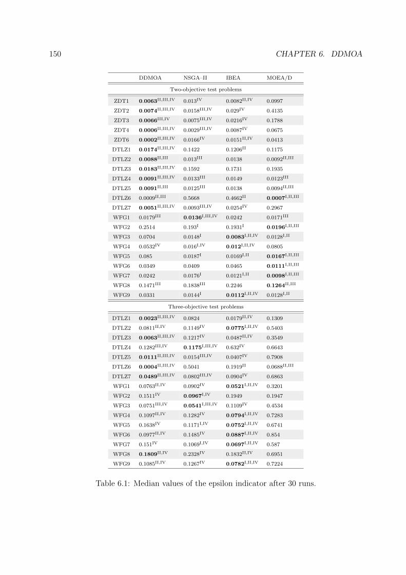
150 CHAPTER 6. DDMOA
DDMOA NSGA–II IBEA MOEA/D
Two-objective test problems
ZDT1 0.0063II,III,IV 0.013IV 0.0082II,IV 0.0997
ZDT2 0.0074II,III,IV 0.0158III,IV 0.029IV 0.4135
ZDT3 0.0066III,IV 0.0075III,IV 0.0216IV 0.1788
ZDT4 0.0006II,III,IV 0.0029III,IV 0.0087IV 0.0675
ZDT6 0.0002II,III,IV 0.0166IV 0.0151II,IV 0.0413
DTLZ1 0.0174II,III,IV 0.1422 0.1206II 0.1175
DTLZ2 0.0088II,III 0.013III 0.0138 0.0092II,III
DTLZ3 0.0183II,III,IV 0.1592 0.1731 0.1935
DTLZ4 0.0091II,III,IV 0.0133III 0.0149 0.0123III
DTLZ5 0.0091II,III 0.0125III 0.0138 0.0094II,III
DTLZ6 0.0009II,III 0.5668 0.4662II 0.0007I,II,III
DTLZ7 0.0051II,III,IV 0.0093III,IV 0.0254IV 0.2967
WFG1 0.0179III 0.0136I,III,IV 0.0242 0.0171III
WFG2 0.2514 0.193I 0.1931I 0.0196I,II,III
WFG3 0.0704 0.0148I 0.0083I,II,IV 0.0128I,II
WFG4 0.0532IV 0.016I,IV 0.012I,II,IV 0.0805
WFG5 0.085 0.0187I 0.0169I,II 0.0167I,II,III
WFG6 0.0349 0.0409 0.0465 0.0111I,II,III
WFG7 0.0242 0.0176I 0.0121I,II 0.0098I,II,III
WFG8 0.1471III 0.1838III 0.2246 0.1264II,III
WFG9 0.0331 0.0144I 0.0112I,II,IV 0.0128I,II
Three-objective test problems
DTLZ1 0.0023II,III,IV 0.0824 0.0179II,IV 0.1309
DTLZ2 0.0811II,IV 0.1149IV 0.0775I,II,IV 0.5403
DTLZ3 0.0063II,III,IV 0.1217IV 0.0487II,IV 0.3549
DTLZ4 0.1282III,IV 0.1175I,III,IV 0.632IV 0.6643
DTLZ5 0.0111II,III,IV 0.0154III,IV 0.0407IV 0.7908
DTLZ6 0.0004II,III,IV 0.5041 0.1919II 0.0688II,III
DTLZ7 0.0489II,III,IV 0.0802III,IV 0.0904IV 0.6863
WFG1 0.0763II,IV 0.0902IV 0.0521I,II,IV 0.3201
WFG2 0.1511IV 0.0967I,IV 0.1949 0.1947
WFG3 0.0751III,IV 0.0541I,III,IV 0.1109IV 0.4534
WFG4 0.1097II,IV 0.1282IV 0.0794I,II,IV 0.7283
WFG5 0.1638IV 0.1171I,IV 0.0752I,II,IV 0.6741
WFG6 0.0977II,IV 0.1485IV 0.0887I,II,IV 0.854
WFG7 0.151IV 0.1069I,IV 0.0697I,II,IV 0.587
WFG8 0.1809II,IV 0.2328IV 0.1832II,IV 0.6951
WFG9 0.1085II,IV 0.1267IV 0.0782I,II,IV 0.7224
Table 6.1: Median values of the epsilon indicator after 30 runs.
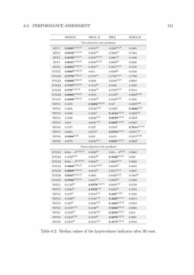
6.3. PERFORMANCE ASSESSMENT 151
DDMOA NSGA–II IBEA MOEA/D
Two-objective test problems
ZDT1 0.2265II,III,IV 0.2315IV 0.2287II,IV 0.3285
ZDT2 0.5576II,III,IV 0.5657IV 0.5639IV 0.7364
ZDT3 0.2758II,III,IV 0.2787III,IV 0.2801IV 0.4499
ZDT4 0.0041II,III,IV 0.0048III,IV 0.0089IV 0.0526
ZDT6 0.2854II,III,IV 0.2951IV 0.2941II,IV 0.3125
DTLZ1 0.0007II,III,IV 0.041 0.0289II 0.0438
DTLZ2 0.7776II,III,IV 0.7791IV 0.7785II,IV 0.7799
DTLZ3 0.0006II,III,IV 0.0394 0.0345II,IV 0.0684
DTLZ4 0.7797II,III,IV 0.7812IV 0.7806 0.7858
DTLZ5 0.779II,III,IV 0.7801IV 0.7797II,IV 0.7814
DTLZ6 0.0083II,III,IV 0.5818 0.4125II 0.0083II,III
DTLZ7 0.3398II,III,IV 0.3442IV 0.3428II,IV 0.5286
WFG1 0.3476 0.3382I,III,IV 0.34I 0.3395I,III
WFG2 0.4645 0.3746I,III 0.3766I 0.3283I,III
WFG3 0.4828 0.4221I 0.4184I,II,IV 0.4202I,II
WFG4 0.7228 0.6892I,IV 0.6873I,II,IV 0.7064I
WFG5 0.645 0.6291I,IV 0.6287I,II,IV 0.6301I
WFG6 0.7477 0.732I 0.7313I 0.7014I,II,III
WFG7 0.6954 0.6775I 0.6753I,II,IV 0.6761I,II
WFG8 0.5968II,III 0.633 0.6415 0.5971II,III
WFG9 0.6779 0.6343I,IV 0.6321I,II,IV 0.6362I
Three-objective test problems
DTLZ1 0.08e− 6II,III,IV 0.0026IV 0.05e− 3II,IV 0.2962
DTLZ2 0.4592II,IV 0.4813IV 0.4429I,II,IV 0.893
DTLZ3 0.08e− 5II,III,IV 0.0043IV 0.0002II,IV 0.5863
DTLZ4 0.4666II,III,IV 0.4721III,IV 0.6256IV 0.8852
DTLZ5 0.8808II,III,IV 0.8818IV 0.8817II,IV 0.9807
DTLZ6 0.0047II,III,IV 0.3865 0.0438II,IV 0.1807II
DTLZ7 0.3763II,III,IV 0.4017IV 0.3876IV 0.9499
WFG1 0.1143IV 0.0778I,III,IV 0.0816I,IV 0.4749
WFG2 0.2022IV 0.0725I,IV 0.2223IV 0.3724
WFG3 0.416IV 0.3514I,IV 0.349I,II,IV 0.7235
WFG4 0.5309IV 0.5104I,IV 0.4587I,II,IV 0.8674
WFG5 0.492IV 0.4602I,IV 0.4263I,II,IV 0.8553
WFG6 0.5735II,IV 0.6106IV 0.5553I,II,IV 0.9292
WFG7 0.4372IV 0.3732I,IV 0.3376I,II,IV 0.814
WFG8 0.5204II,IV 0.5579IV 0.5075I,II,IV 0.8991
WFG9 0.5372IV 0.5214I,IV 0.4717I,II,IV 0.8794
Table 6.2: Median values of the hypervolume indicator after 30 runs.

152 CHAPTER 6. DDMOA
tested problems. In terms of robustness, the best algorithm is also DDMOA. Figure 6.7(b)
shows that the most accurate algorithm is DDMOA, providing the best median values of
the hypervolume indicator in 49% of the tested problems. In terms of robustness, the best
algorithm is again DDMOA.
Table 6.1 presents the statistical comparison and the median values of the epsilon
indicator. The superscripts I, II, III and IV indicate whether the respective algorithm
performs significantly better than DDMOA, NSGA–II, IBEA, and MOEA/D, respectively.
The best value in each row is marked bold (the lower the better). DDMOA outperforms
the other algorithms on ZDT and the majority of the two and three-objective DTLZ test
problems. On the two-objective WFG test problems, the best performance is achieved by
MOEA/D that provides the best median values of the epsilon indicator in 5 out of 9 test
problems. On the three-objective WFG test problems, IBEA has the best performance,
providing the best median values of the epsilon indicator in 6 out of 9 test problems.
Table 6.2 shows the statistical comparison and the median values of the hypervolume
indicator. The superscripts I, II, III and IV indicate whether the respective algorithm
performs significantly better than DDMOA, NSGA–II, IBEA, and MOEA/D, respectively.
The best value in each row is marked bold (the lower the better). DDMOA outperforms
the other algorithms on the two-objective ZDT and DTLZ test problems, providing sig-
nificantly better values of the hypervolume indicator than all other considered algorithms.
IBEA performs significantly better than the other algorithms on the 5 two-objective WFG
test problems. On the three-objective WFG3-9 test problems, IBEA gives significantly
better results in terms of the hypervolume indicator than the other algorithms. The domi-
nance of IBEA on WFG test problems in terms of the hypervolume can be explained by the
fact that it is the only algorithm that attempts to maximize the cumulative hypervolume
covered by nondominated solutions.
Figures 6.8–6.12 present approximation sets with the best hypervolume values found
by DDMOA in 30 runs. In Figures 6.8, 6.9, and 6.10, it can be seen that DDMOA reaches
the Pareto fronts for all the ZDT and DTLZ test problems, giving well-distributed sets of
solutions in the objective space. From Figure 6.11, one can see that DDMOA performs
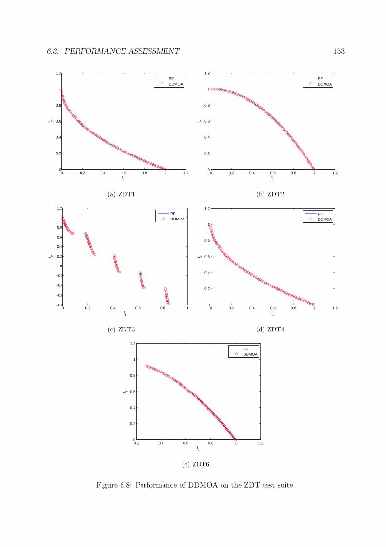
6.3. PERFORMANCE ASSESSMENT 153
0 0.2 0.4 0.6 0.8 1 1.20
0.2
0.4
0.6
0.8
1
1.2
f1
f 2
PFDDMOA
(a) ZDT1
0 0.2 0.4 0.6 0.8 1 1.20
0.2
0.4
0.6
0.8
1
1.2
f1
f 2
PFDDMOA
(b) ZDT2
0 0.2 0.4 0.6 0.8 1−0.8
−0.6
−0.4
−0.2
0
0.2
0.4
0.6
0.8
1
1.2
f1
f 2
PFDDMOA
(c) ZDT3
0 0.2 0.4 0.6 0.8 1 1.20
0.2
0.4
0.6
0.8
1
1.2
f1
f 2
PFDDMOA
(d) ZDT4
0.2 0.4 0.6 0.8 1 1.20
0.2
0.4
0.6
0.8
1
1.2
f1
f 2
PFDDMOA
(e) ZDT6
Figure 6.8: Performance of DDMOA on the ZDT test suite.

154 CHAPTER 6. DDMOA
0 0.1 0.2 0.3 0.4 0.5 0.60
0.1
0.2
0.3
0.4
0.5
0.6
f1
f 2
PFDDMOA
(a) DTLZ1
0 0.2 0.4 0.6 0.8 1 1.20
0.2
0.4
0.6
0.8
1
1.2
f1
f 2
PFDDMOA
(b) DTLZ2
0 0.2 0.4 0.6 0.8 1 1.20
0.2
0.4
0.6
0.8
1
1.2
f1
f 2
PFDDMOA
(c) DTLZ3
0 0.2 0.4 0.6 0.8 1 1.20
0.2
0.4
0.6
0.8
1
1.2
f1
f 2
PFDDMOA
(d) DTLZ4
0 0.2 0.4 0.6 0.8 1 1.20
0.2
0.4
0.6
0.8
1
1.2
f1
f 2
PFDDMOA
(e) DTLZ5
0 0.2 0.4 0.6 0.8 1 1.20
0.2
0.4
0.6
0.8
1
1.2
f1
f 2
PFDDMOA
(f) DTLZ6

6.3. PERFORMANCE ASSESSMENT 155
0 0.2 0.4 0.6 0.8 12.2
2.4
2.6
2.8
3
3.2
3.4
3.6
3.8
4
4.2
f1
f 2
PFDDMOA
(g) DTLZ7
Figure 6.9: Performance of DDMOA on the two-objective DTLZ test suite.
00.2
0.40.6
0.8
00.2
0.40.6
0.8
0
0.2
0.4
0.6
0.8
f1f2
f 3
PFDDMOA
(a) DTLZ1
0
0.5
1
1.5
0
0.5
1
1.5
0
0.5
1
1.5
f1f2
f 3
PFDDMOA
(b) DTLZ2

156 CHAPTER 6. DDMOA
0
0.5
1
1.5
0
0.5
1
1.5
0
0.5
1
1.5
f1f2
f 3
PFDDMOA
(c) DTLZ3
0
0.5
1
1.5
0
0.5
1
1.5
0
0.5
1
1.5
f1f2
f 3
PFDDMOA
(d) DTLZ4
0
0.2
0.4
0.6
0.8
00.2
0.40.6
0.8
0
0.5
1
1.5
f1f2
f 3
PFDDMOA
(e) DTLZ5
0
0.2
0.4
0.6
0.8
00.2
0.40.6
0.8
0
0.5
1
1.5
f1f2
f 3
PFDDMOA
(f) DTLZ6
0
0.2
0.4
0.6
0.8
1
00.2
0.40.6
0.81
2
3
4
5
6
f1f2
f 3
PFDDMOA
(g) DTLZ7
Figure 6.10: Performance of DDMOA on the three-objective DTLZ test suite.
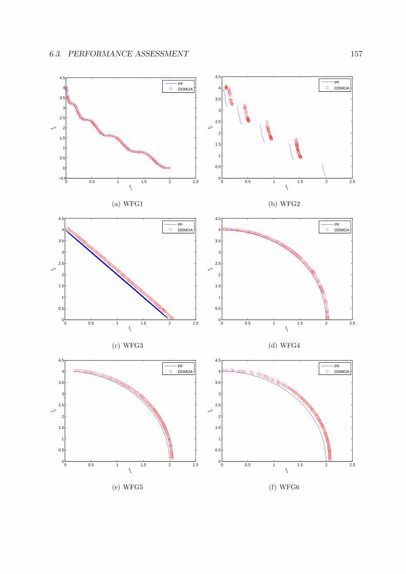
6.3. PERFORMANCE ASSESSMENT 157
0 0.5 1 1.5 2 2.5−0.5
0
0.5
1
1.5
2
2.5
3
3.5
4
4.5
f1
f 2
PFDDMOA
(a) WFG1
0 0.5 1 1.5 2 2.50
0.5
1
1.5
2
2.5
3
3.5
4
4.5
f1
f 2
PFDDMOA
(b) WFG2
0 0.5 1 1.5 2 2.50
0.5
1
1.5
2
2.5
3
3.5
4
4.5
f1
f 2
PFDDMOA
(c) WFG3
0 0.5 1 1.5 2 2.50
0.5
1
1.5
2
2.5
3
3.5
4
4.5
f1
f 2
PFDDMOA
(d) WFG4
0 0.5 1 1.5 2 2.50
0.5
1
1.5
2
2.5
3
3.5
4
4.5
f1
f 2
PFDDMOA
(e) WFG5
0 0.5 1 1.5 2 2.50
0.5
1
1.5
2
2.5
3
3.5
4
4.5
f1
f 2
PFDDMOA
(f) WFG6

158 CHAPTER 6. DDMOA
0 0.5 1 1.5 2 2.50
0.5
1
1.5
2
2.5
3
3.5
4
4.5
f1
f 2
PFDDMOA
(g) WFG7
0 0.5 1 1.5 2 2.50
0.5
1
1.5
2
2.5
3
3.5
4
4.5
f1
f 2
PFDDMOA
(h) WFG8
0 0.5 1 1.5 2 2.50
0.5
1
1.5
2
2.5
3
3.5
4
4.5
f1
f 2
PFDDMOA
(i) WFG9
Figure 6.11: Performance of DDMOA on the two-objective WFG test suite.
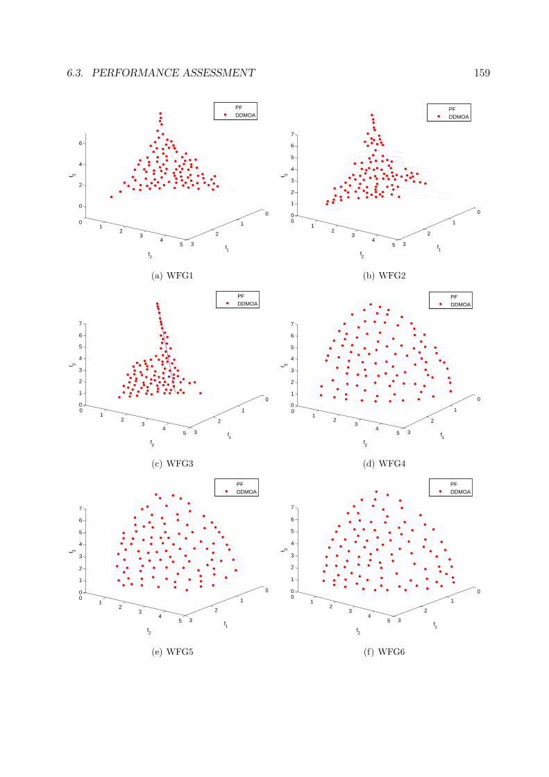
6.3. PERFORMANCE ASSESSMENT 159
0
1
2
3
01
23
45
0
2
4
6
f1f2
f 3
PFDDMOA
(a) WFG1
0
1
2
3
01
23
45
0
1
2
3
4
5
6
7
f1f2
f 3
PFDDMOA
(b) WFG2
0
1
2
3
01
23
45
0
1
2
3
4
5
6
7
f1f2
f 3
PFDDMOA
(c) WFG3
0
1
2
3
01
23
45
0
1
2
3
4
5
6
7
f1f2
f 3
PFDDMOA
(d) WFG4
0
1
2
3
01
23
45
0
1
2
3
4
5
6
7
f1f2
f 3
PFDDMOA
(e) WFG5
0
1
2
3
01
23
45
0
1
2
3
4
5
6
7
f1f2
f 3
PFDDMOA
(f) WFG6

160 CHAPTER 6. DDMOA
0
1
2
3
01
23
45
0
1
2
3
4
5
6
7
f1f2
f 3
PFDDMOA
(g) WFG7
0
1
2
3
01
23
45
0
1
2
3
4
5
6
7
f1f2
f 3
PFDDMOA
(h) WFG8
0
1
2
3
01
23
45
0
1
2
3
4
5
6
7
f1f2
f 3
PFDDMOA
(i) WFG9
Figure 6.12: Performance of DDMOA on the three-objective WFG test suite.
poorly on the majority of the two-objective WFG test problems. However, adequate Pareto
front approximations are achieved by DDMOA on WFG1,4,7. Although DDMOA performs
poorly on the WFG8 test problem, from Table 6.2, one can see that DDMOA provides the
best median value of the hypervolume indicator, being significantly better than NSGA-II
and IBEA on this problem. In Figure 6.12, it can be observed that DDMOA is able to
find adequate Pareto front approximations for all the three-objective WFG test problems,
except for the WFG3 test problem.

6.4. SUMMARY 161
6.4 Summary
The review of existing approaches for MO given in Chapter 3 shows that the majority
of state-of-the-art EMO algorithms use variation operators initially designed for single-
objective EAs. Since the particularities of multiobjective optimization are often not taken
into consideration, some operators that are suitable for single-objective optimization may
lead to a poor performance in the presence of multiple conflicting objectives. Although
combinations of classical methods and evolutionary algorithms often outperform traditional
EAs in single-objective optimization, such methods still remain to be an under-explored
research area in multiobjective optimization.
This chapter introduces a new hybrid multiobjective evolutionary algorithm, termed
DDMOA. DDMOA combines different concepts from single-objective and multiobjective
optimization. The main idea of generating new candidate solutions is borrowed from
Timmel’s method for MO. To overcome the limitations related to the use of gradients,
descent directions are calculated. Found descent directions are stored in the search matrix
of each individual in the population. This way, search matrices store information about
fitness landscape in the vicinity of each population member. The computation of descent
directions is performed by a pattern search method. To perform the search in the objective
space, the widely used Pareto dominance-based environmental selection is adopted from
EMO algorithms.
The performed experimental studies show that DDMOA is a competitive multiobjective
optimizer. The ability of DDMOA to outperform state-of-the-art EMO algorithms on
multimodal problems is directly related to its hybrid reproduction operator. The obtained
results clearly indicate that the proposed approach is a promising direction for further
research.

162 CHAPTER 6. DDMOA

Chapter 7
Generalized Descent
Directions-Guided Multiobjective
Algorithm
7.1 Introduction
The previous chapter introduces a multiobjective evolutionary algorithm with a hybrid
reproduction operator, which is based on the idea of Timmel’s method for generating
new candidate solutions. Although the algorithm exhibits a competitive performance in
the comparative studies with some state-of-the-art MOEAs, several issues are identified
as potential weaknesses of DDMOA. In particular, in DDMOA the population consists
only of nondominated individuals that can cause only a few or even one individual being
present in the current population. That can severely deteriorate the performance of the
algorithm. Since a few individuals are present in the population, it becomes difficult to
escape from suboptimal regions of the search space. Another weakness is that the original
DDMOA is not applicable to many-objective problems. Moreover, when the number of
objectives is increased, finding descent directions for all objectives using local search may
be computationally expensive.
163
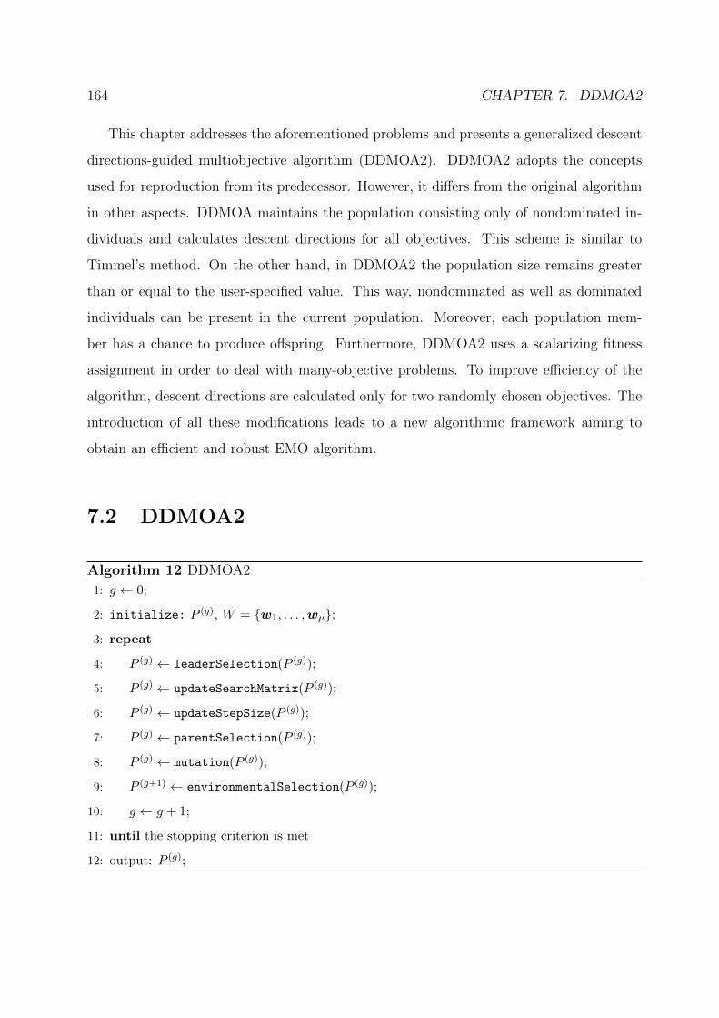
164 CHAPTER 7. DDMOA2
This chapter addresses the aforementioned problems and presents a generalized descent
directions-guided multiobjective algorithm (DDMOA2). DDMOA2 adopts the concepts
used for reproduction from its predecessor. However, it differs from the original algorithm
in other aspects. DDMOA maintains the population consisting only of nondominated in-
dividuals and calculates descent directions for all objectives. This scheme is similar to
Timmel’s method. On the other hand, in DDMOA2 the population size remains greater
than or equal to the user-specified value. This way, nondominated as well as dominated
individuals can be present in the current population. Moreover, each population mem-
ber has a chance to produce offspring. Furthermore, DDMOA2 uses a scalarizing fitness
assignment in order to deal with many-objective problems. To improve efficiency of the
algorithm, descent directions are calculated only for two randomly chosen objectives. The
introduction of all these modifications leads to a new algorithmic framework aiming to
obtain an efficient and robust EMO algorithm.
7.2 DDMOA2
Algorithm 12 DDMOA2
1: g ← 0;
2: initialize: P (g), W = w1, . . . ,wµ;
3: repeat
4: P (g) ← leaderSelection(P (g));
5: P (g) ← updateSearchMatrix(P (g));
6: P (g) ← updateStepSize(P (g));
7: P (g) ← parentSelection(P (g));
8: P (g) ← mutation(P (g));
9: P (g+1) ← environmentalSelection(P (g));
10: g ← g + 1;
11: until the stopping criterion is met
12: output: P (g);
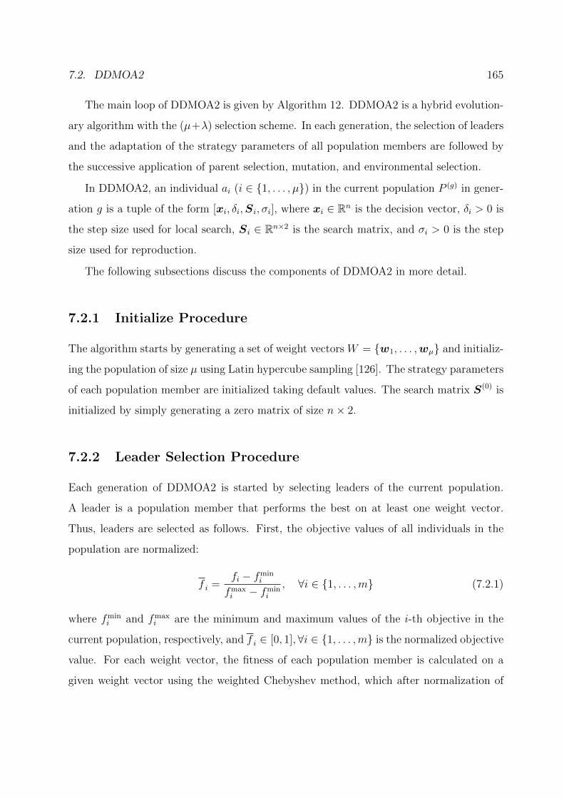
7.2. DDMOA2 165
The main loop of DDMOA2 is given by Algorithm 12. DDMOA2 is a hybrid evolution-
ary algorithm with the (µ+λ) selection scheme. In each generation, the selection of leaders
and the adaptation of the strategy parameters of all population members are followed by
the successive application of parent selection, mutation, and environmental selection.
In DDMOA2, an individual ai (i ∈ 1, . . . , µ) in the current population P (g) in gener-
ation g is a tuple of the form [xi, δi,Si, σi], where xi ∈ Rn is the decision vector, δi > 0 is
the step size used for local search, Si ∈ Rn×2 is the search matrix, and σi > 0 is the step
size used for reproduction.
The following subsections discuss the components of DDMOA2 in more detail.
7.2.1 Initialize Procedure
The algorithm starts by generating a set of weight vectors W = w1, . . . ,wµ and initializ-
ing the population of size µ using Latin hypercube sampling [126]. The strategy parameters
of each population member are initialized taking default values. The search matrix S(0) is
initialized by simply generating a zero matrix of size n× 2.
7.2.2 Leader Selection Procedure
Each generation of DDMOA2 is started by selecting leaders of the current population.
A leader is a population member that performs the best on at least one weight vector.
Thus, leaders are selected as follows. First, the objective values of all individuals in the
population are normalized:
f i =fi − fmin
i
fmaxi − fmin
i
, ∀i ∈ 1, . . . ,m (7.2.1)
where fmini and fmax
i are the minimum and maximum values of the i-th objective in the
current population, respectively, and f i ∈ [0, 1],∀i ∈ 1, . . . ,m is the normalized objective
value. For each weight vector, the fitness of each population member is calculated on a
given weight vector using the weighted Chebyshev method, which after normalization of

166 CHAPTER 7. DDMOA2
objectives can be defined as:
ffitness = max1≤i≤m
wi f i(x) (7.2.2)
where ffitness is the fitness of the population member x on the weight vector w. An
individual having the best fitness on a given weight vector is a leader. It should be noted
that one leader can have the best fitness value on several weight vectors.
7.2.3 Update Search Matrix Procedure
After selecting leader individuals, the search matrices of all individuals in the current pop-
ulation are updated in updateSearchMatrix procedure. In DDMOA2, descent directions
are calculated only for two randomly chosen objectives, regardless of the dimensionality
of the objective space. Thus, the search matrix of each population member contains two
columns that store descent directions for these randomly chosen objectives. The motiva-
tion behind finding descend directions only for two instead of all objectives is that in the
presence of a large number of objectives calculating descend directions for all objectives
using local search may become computationally expensive.
In the beginning of updateSearchMatrix procedure, two objectives are chosen at ran-
dom, and only leaders of the current population are considered while all the other indi-
viduals are temporarily discarded. Thereafter, for the first chosen objective, the resulting
population is sorted in ascending order and partitioned into α equal parts. Thus, α sub-
populations are defined in order to promote different reference points for the computation
of descent directions. It follows that in each subpopulation, a representative individual ar is
selected. A representative of the subpopulation is a solution with the smallest value of the
corresponding objective function among other solutions in the subpopulation and δ > δtol.
Thus, if the solution with the smallest value of the corresponding objective has δ ≤ δtol
then the solution with the second smallest value is selected as representative and so on.
After that, a descent direction for the corresponding objective function is computed for the
representative using coordinate search [175]. During coordinate search, the step size δ of
the representative is reduced if no decrease in the objective function value is found. Each

7.2. DDMOA2 167
time a trial solution is calculated, this solution is compared with the current population. If
this trial solution has a smaller value for at least one objective compared with each member
of the current population then it is added to the population, assuming the default values of
the strategy parameters. When a descent direction sr for the subpopulation representative
is found, descent directions for all other subpopulation members are computed as follows:
si = xr − xi + sr, (7.2.3)
where si is the descent direction for the i-th subpopulation member, xi is the decision
vector of the i-th subpopulation member, xr is the subpopulation representative, and sr is
the descent direction for the representative. The calculated descent directions are stored
in the first column of the search matrices of the corresponding individuals. Thereafter, the
same procedure for finding descent directions is performed for the second chosen objective
and the results are stored in the second column of the search matrices.
After the search matrices of leaders of the current population are updated, the search
matrices of all other population members need to be updated. For this purpose, a simple
stochastic procedure is used. For each non-leader individual, a leader is randomly chosen
and this leader shares its search matrix, i.e., non-leader individual’s search matrix is equal
to the selected leader’s search matrix. At the end of updateSearchMatrix procedure, the
search matrices of all population members are updated. Since some promising solutions
satisfying the aforementioned conditions are added to the population during coordinate
search, at the end of this procedure, the population size is usually greater than µ.
7.2.4 Update Step Size Procedure
Before generating offspring, the step size of each population member needs to be updated.
However, there is no common rule to update the step size σ, but it must be done carefully
to ensure convergence to the Pareto set, starting from a larger value at the beginning
and gradually reducing it during the generations. DDMOA2 uses the following rule for

168 CHAPTER 7. DDMOA2
updating the step size of each population member:
σ = maxexp(τN(0, 1))σ(1− 3 funEval
maxEval)
0 , δtol (7.2.4)
where τ is the learning parameter (τ = 1/√
2n), N(0, 1) is a random number sampled from
the normal distribution with mean 0 and standard deviation 1, σ0 is the initial value of
the step size, funEval is the current number of function evaluations, and maxEval is the
maximum number of function evaluations. The idea here is to exponentially reduce the
step size depending on the current number of function evaluations and multiply it by a
scaling factor, thereby obtaining different step size values among the population members.
7.2.5 Parent Selection Procedure
In each generation, λ offspring individuals are generated by mutating the correspondent
parent. The decision on how many offspring are produced from each population member is
made in parentSelection procedure. At the beginning, it is assumed that none offspring
is generated by each individual. Then, binary tournament selection based on scalarizing
fitness is performed to identify which population members will be mutated in order to
produce offspring. This selection process is based on the idea proposed in [97] and fosters
promising individuals to produce more offspring.
The procedure starts by normalizing the objective values of all individuals in the pop-
ulation as defined in (7.2.1). Then, the selection process is performed in two stages. In the
first stage, only leaders of the current population are considered. For each weight vector,
two individuals are randomly selected and the fitness of the corresponding individual is
calculated as defined in (7.2.2). The individual having smallest fitness value is a winner
and the number of times it is mutated is augmented by one. Thereafter, all leaders are
removed from the population and, for each weight vector, binary tournament selection is
performed on the resulting population in the same way as it is done for leaders. It should
be noted that some population members might be mutated several times, as a result of
this procedure, while others will not produce any offspring at all.

7.2. DDMOA2 169
7.2.6 Mutation Procedure
After identifying which population members have to be mutated, offspring are generated
in mutation procedure. For the corresponding individual, the mutation is performed as
follows:
x′ = x+ σS ν (7.2.5)
where σ is the step size, S is the search matrix and ν is a column vector of random numbers
sampled from the uniform distribution (∀i ∈ 1, 2 : νi ∼ U(0, 1)). To guarantee that each
new solution x′ = (x′1, . . . , x′n)T belongs to Ω, projection is applied to each component of
the decision vector: x′ = minmaxx′, l,u. After offspring x′ is repaired, it is evaluated
and added to the population.
7.2.7 Environmental Selection Procedure
At the end of each generation, µ fittest individuals are selected from the enlarged population
in environmentalSelection procedure. DDMOA2 uses the selection mechanism proposed
in [92].
First, the objective values of all individuals are normalized as defined in (7.2.1). Next,
the following steps are performed:
1. matrix M is calculated, which stores metrics for each population member on each
weight vector (for each population member, a metric on a corresponding weight vector
is computed as defined in (7.2.2));
2. for each column (weight vector), the minimum and second smallest metric value are
found;
3. for each column, metric values are scaled by the minimum value found, except for
the row which gave the minimum value. This result is scaled by the second lowest
value;

170 CHAPTER 7. DDMOA2
4. for each row (population member), the minimum scaled value is found, this value
represents individual’s fitness;
5. the resulting column vector is sorted, and µ individuals with the smallest fitness
values are selected.
Normalizing objective values allows to cope with differently scaled objectives, while the
weighted Chebyshev method can find optimal solutions in convex and nonconvex regions
of the Pareto front.
7.3 Performance Assessment
In this section, the performance of DDMOA2 is investigated. First, the algorithm is com-
pared with its predecessor on a set of two and three-objective test instances in order to
study the impact of the introduced modifications. Then, the performance of DDMOA2
on many-objective problems is studied and compared with some state-of-the-art many-
objective optimizers. Once again, the main feature under concern is the proposed hybrid
reproduction operator and its viability within a new algorithmic framework adopted by
DDMOA2.
7.3.1 Preliminary Experiments
In this study, DDMOA2 is compared with its predecessor DDMOA and state-of-the-art
EMO algorithm NSGA-II [46] on the WFG test suite [88]. The outcomes of the algorithms
are assessed using the GD and IGD indicators. Furthermore, the overall performance of the
algorithms is shown using performance profiles, and the pairwise statistical comparison is
performed using the nonparametric Wilcoxon rank-sum test performed at the significance
level of α = 0.05.
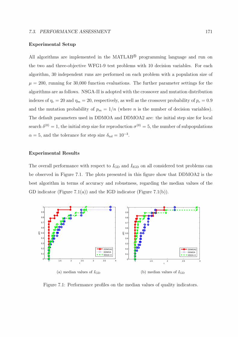
7.3. PERFORMANCE ASSESSMENT 171
Experimental Setup
All algorithms are implemented in the MATLAB R© programming language and run on
the two and three-objective WFG1-9 test problems with 10 decision variables. For each
algorithm, 30 independent runs are performed on each problem with a population size of
µ = 200, running for 30,000 function evaluations. The further parameter settings for the
algorithms are as follows. NSGA-II is adopted with the crossover and mutation distribution
indexes of ηc = 20 and ηm = 20, respectively, as well as the crossover probability of pc = 0.9
and the mutation probability of pm = 1/n (where n is the number of decision variables).
The default parameters used in DDMOA and DDMOA2 are: the initial step size for local
search δ(0) = 1, the initial step size for reproduction σ(0) = 5, the number of subpopulations
α = 5, and the tolerance for step size δtol = 10−3.
Experimental Results
The overall performance with respect to IGD and IIGD on all considered test problems can
be observed in Figure 7.1. The plots presented in this figure show that DDMOA2 is the
best algorithm in terms of accuracy and robustness, regarding the median values of the
GD indicator (Figure 7.1(a)) and the IGD indicator (Figure 7.1(b)).
1 1.5 2 2.5 3 3.5 40
0.1
0.2
0.3
0.4
0.5
0.6
0.7
0.8
0.9
1
τ
ρ(τ)
DDMOA2DDMOANSGA−II
(a) median values of IGD
1 1.5 2 2.5 30
0.1
0.2
0.3
0.4
0.5
0.6
0.7
0.8
0.9
1
τ
ρ(τ)
DDMOA2DDMOANSGA−II
(b) median values of IGD
Figure 7.1: Performance profiles on the median values of quality indicators.

172 CHAPTER 7. DDMOA2
DDMOA2 DDMOA NSGA-II
2-objectives
WFG1 0.0052 0.0048I,III 0.0051
WFG2 0.0183II 0.0502 0.0133I,II
WFG3 0.0037II,III 0.0052 0.0047
WFG4 0.0191 0.0192 0.0096I,II
WFG5 0.0630II,III 0.0640 0.0639
WFG6 0.0265III 0.0288III 0.0709
WFG7 0.0051 0.0040I 0.0041I
WFG8 0.1892III 0.1984 0.2272
WFG9 0.0177 0.0125I 0.0132I
3-objectives
WFG1 0.0459II,III 0.0720 0.0709
WFG2 0.0845II,III 0.2080 0.1388II
WFG3 0.2006II,III 0.4940III 0.5185
WFG4 0.0867II,III 0.1278 0.1186II
WFG5 0.0995II,III 0.1362 0.1228II
WFG6 0.0762II,III 0.1268III 0.1688
WFG7 0.0733II,III 0.0908 0.0843II
WFG8 0.2090II,III 0.3556III 0.3978
WFG9 0.0721II,III 0.0858 0.0829II
Table 7.1: Statistical comparison
in terms of IGD.
DDMOA2 DDMOA NSGA-II
2-objectives
WFG1 0.007II,III 0.0081 0.0076II
WFG2 0.0169II 0.0267 0.0164II
WFG3 0.0067II,III 0.0094 0.0085II
WFG4 0.0149II 0.0175 0.0078I,II
WFG5 0.0649II,III 0.0653 0.0653
WFG6 0.0243III 0.0243III 0.0709
WFG7 0.0075II,III 0.0083 0.0080II
WFG8 0.1373 0.1366 0.1495
WFG9 0.0125 0.0125 0.0118
3-objectives
WFG1 0.2252 0.1757I 0.1359I,II
WFG2 0.2469 0.2256I 0.1580I,II
WFG3 0.0258II,III 0.0390III 0.0504
WFG4 0.1840II,III 0.2169 0.1980II
WFG5 0.2075II,III 0.2447 0.2189II
WFG6 0.1921II,III 0.2706 0.2512II
WFG7 0.1882II,III 0.2447 0.1938II
WFG8 0.4607II,III 0.5790 0.5331II
WFG9 0.1895II,III 0.2208 0.1974II
Table 7.2: Statistical comparison
in terms of IIGD.
Tables 7.1 and 7.2 show the median values of the generational distance indicator and
the inverted generational distance indicator, respectively, over 30 runs. The superscripts
I, II and III indicate whether the respective algorithm performs significantly better than
DDMOA2, DDMOA, and NSGA–II, respectively. The best value in each row is marked
bold (the lower the better). For the two-objective problems, DDMOA2 achieves the best

7.3. PERFORMANCE ASSESSMENT 173
values of both quality indicators on the four test problems, always being significantly bet-
ter than NSGA–II. On the majority of the problems DDMOA2 is significantly better than
DDMOA. With respect to the three-objective problems, the new DDMOA2 completely out-
performs the other algorithms regarding IGD. Concerning IIGD, DDMOA2 is significantly
better on 7 out of 9 WFG test problems.
From the discussed results, it becomes clear that the new DDMOA2 performs generally
better than its predecessor DDMOA. The achieved outperformance can be attributed to
the fact that in DDMOA2 the population is constituted not only of nondominated solutions
as well as all population members can generate offspring. Furthermore, it is shown that
the proposed approach based on finding descent directions only for two randomly chosen
objectives is able to guide efficiently the search.
Additionally, Figures 7.2 and 7.3 show approximation sets with the best values of IIGD
obtained by DDMOA2 on the two and three-objective WFG test problems. It can be seen
that DDMOA2 is able to obtain adequate Pareto front approximations on the majority
of the two-objective test problems (Figures 7.2). However, on the WFG5 problem, the
approximation set is not close enough to the true Pareto front (Figure 7.2(e)). Also,
a poor performance is observed on the WGF8 test problem (Figure 7.2(h)). This is a
difficult nonseparable problem [88], on which many algorithms fail to obtain a good Pareto
0 0.5 1 1.5 2 2.5−0.5
0
0.5
1
1.5
2
2.5
3
3.5
4
4.5
f1
f 2
PFDDMOA2
(a) WFG1
0 0.5 1 1.5 2 2.50
0.5
1
1.5
2
2.5
3
3.5
4
4.5
f1
f 2
PFDDMOA2
(b) WFG2

174 CHAPTER 7. DDMOA2
0 0.5 1 1.5 2 2.50
0.5
1
1.5
2
2.5
3
3.5
4
4.5
f1
f 2
PFDDMOA2
(c) WFG3
0 0.5 1 1.5 2 2.50
0.5
1
1.5
2
2.5
3
3.5
4
4.5
f1
f 2
PFDDMOA2
(d) WFG4
0 0.5 1 1.5 2 2.50
0.5
1
1.5
2
2.5
3
3.5
4
4.5
f1
f 2
PFDDMOA2
(e) WFG5
0 0.5 1 1.5 2 2.50
0.5
1
1.5
2
2.5
3
3.5
4
4.5
f1
f 2
PFDDMOA2
(f) WFG6
0 0.5 1 1.5 2 2.50
0.5
1
1.5
2
2.5
3
3.5
4
4.5
f1
f 2
PFDDMOA2
(g) WFG7
0 0.5 1 1.5 2 2.50
0.5
1
1.5
2
2.5
3
3.5
4
4.5
f1
f 2
PFDDMOA2
(h) WFG8
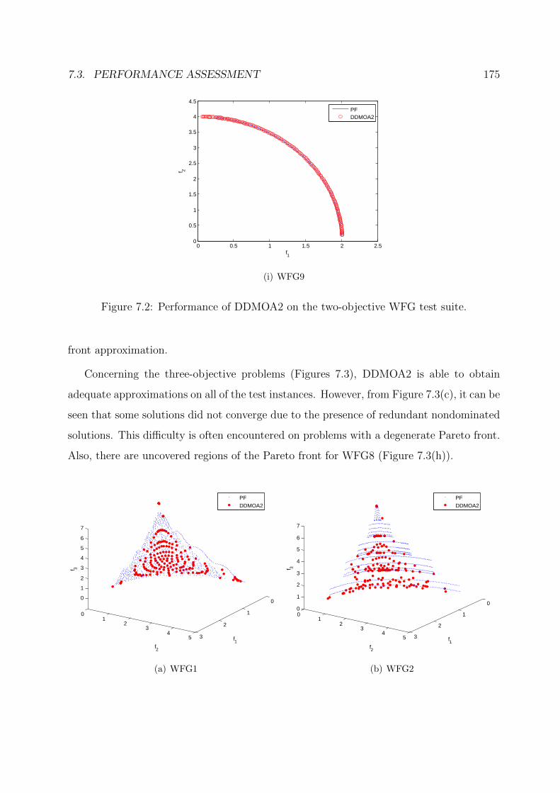
7.3. PERFORMANCE ASSESSMENT 175
0 0.5 1 1.5 2 2.50
0.5
1
1.5
2
2.5
3
3.5
4
4.5
f1
f 2
PFDDMOA2
(i) WFG9
Figure 7.2: Performance of DDMOA2 on the two-objective WFG test suite.
front approximation.
Concerning the three-objective problems (Figures 7.3), DDMOA2 is able to obtain
adequate approximations on all of the test instances. However, from Figure 7.3(c), it can be
seen that some solutions did not converge due to the presence of redundant nondominated
solutions. This difficulty is often encountered on problems with a degenerate Pareto front.
Also, there are uncovered regions of the Pareto front for WFG8 (Figure 7.3(h)).
0
1
2
3
01
23
45
0
1
2
3
4
5
6
7
f1f2
f 3
PFDDMOA2
(a) WFG1
0
1
2
3
01
23
45
0
1
2
3
4
5
6
7
f1f2
f 3
PFDDMOA2
(b) WFG2

176 CHAPTER 7. DDMOA2
0
1
2
3
01
23
45
0
1
2
3
4
5
6
7
f1f2
f 3
PFDDMOA2
(c) WFG3
0
1
2
3
01
23
45
0
1
2
3
4
5
6
7
f1f2
f 3
PFDDMOA2
(d) WFG4
0
1
2
3
01
23
45
0
1
2
3
4
5
6
7
f1f2
f 3
PFDDMOA2
(e) WFG5
0
1
2
3
01
23
45
0
1
2
3
4
5
6
7
f1f2
f 3
PFDDMOA2
(f) WFG6
0
1
2
3
01
23
45
0
1
2
3
4
5
6
7
f1f2
f 3
PFDDMOA2
(g) WFG7
0
1
2
3
01
23
45
0
1
2
3
4
5
6
7
f1f2
f 3
PFDDMOA2
(h) WFG8

7.3. PERFORMANCE ASSESSMENT 177
0
1
2
3
01
23
45
0
1
2
3
4
5
6
7
f1f2
f 3
PFDDMOA2
(i) WFG9
Figure 7.3: Performance of DDMOA2 on the three-objective WFG test suite.
7.3.2 Intermediate Summary
In the above discussed experiments, the performance of a generalized descent directions-
guided multiobjective algorithm DDMOA2 is investigated and compared with its predeces-
sor DDMOA. Both algorithms employ the same reproduction operator and general prin-
ciples for computing descent directions. However, they differ significantly in some other
components.
DDMOA2 does not rely on the concept of the Pareto dominance. Its parent and en-
vironmental selections are based on the scalarizing fitness assignment. DDMOA2 always
maintains a number of individuals in the population that is not less than µ. This leads
to the need for selecting promising individuals in the population to apply a local search
procedure. Contrary to DDMOA, DDMOA2 uses the local search procedure to find de-
scent directions only for two randomly chosen objectives. Furthermore, in DDMOA2 all
individuals in the population have a chance to produce offspring.
The experimental results show that DDMOA2 generally outperforms its predecessor
DDMOA, regarding the convergence to the Pareto front and the diversity of the obtained
solutions. At the same time, DDMOA2 performs better than representative state-of-the-art
NSGA–II in terms of both considered quality indicators.
178 CHAPTER 7. DDMOA2
7.3.3 Further Experiments
In the following, the performance of DDMOA2 is studied on many-objective problems. The
introduction of a scalarizing fitness assignment into the framework of descent directions-
guided multiobjective algorithm is a major motivation for solving this sort of problems.
The performance of DDMOA2 is compared with that produced by the state-of-the-art
many-objective optimizers IBEA [198] and MOEA/D [123] on the DTLZ test suite [50]
with 30 decision variables having between 2 and 8 objectives.
Experimental Setup
DDMOA2 and MOEA/D are implemented in the MATLAB R© programming language,
IBEA is used within the PISA [16] framework. For each algorithm, 30 independent runs
are performed on each problem with a population size of µ = 200, running for 60,000 func-
tion evaluations. The further parameter settings for the algorithms are as follows. IBEA
is adopted with the crossover and mutation distribution indexes of ηc = 20 and ηm = 20,
respectively, as well as the crossover probability of pc = 0.9 and the mutation probabil-
ity of pm = 1/n (where n is the number of decision variables). The control parameters
used in MOEA/D are: the number of weight vectors in the neighborhood of each weight
vector T = 20, the probability that the parent selected from the neighborhood δ = 0.9,
the maximum number of solutions replaced by each child solution nr = 2. Settings for
the DE operator are: CR = 0.15 and F = 0.5, the mutation probability of pm = 1/n and
the mutation distribution index of ηm = 20 are used in the polynomial mutation operator.
The parameters used in DDMOA2 are: the initial step size for local search δ(0) = 0.4, the
initial step size for reproduction σ(0) = 5, the number of subpopulations α = 5, and the
tolerance for step size δtol = 10−3.
Dealing with many-objective problems often requires an additional search pressure ei-
ther in the decision or the objective space. The scalarizing fitness assignment used by
DDMOA2 ensures the selection pressure during the evolutionary process. To increase the
search pressure in the decision space, an additional condition for the acceptance of descent

7.3. PERFORMANCE ASSESSMENT 179
1f
2f
rx
rr sx
rs
2x
3x4x
5x
(a) without additional condition
1f
2f
rx
rr sx
rs2x
3x4x
5x
(b) with additional condition
1f
2f
rxrs
2x
3x4x
5x
(c) resulted descent directions
Figure 7.4: Computation of descent directions.
directions is introduced. Thus, descent direction sr for representative xr is accepted during
local search if trail solution xr + sr is not worse in all objectives than xr, and direction sr
leads to the decrease of the corresponding objective (objective for which descent direction
is calculated).
Figure 7.4 allows to better understand this procedure. In which a subpopulation is
presented and local search is used to find descent directions with respect to f1. Simply
calculating the descent direction sr for subpopulation representative xr, a descent direction
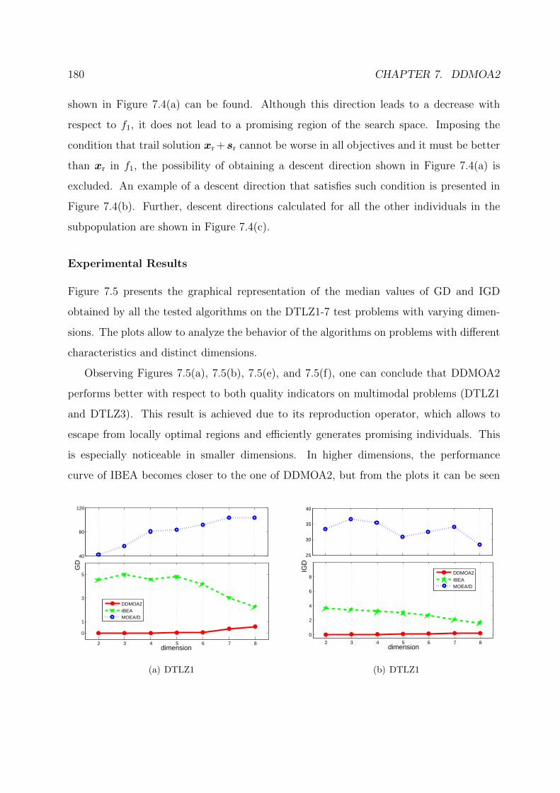
180 CHAPTER 7. DDMOA2
shown in Figure 7.4(a) can be found. Although this direction leads to a decrease with
respect to f1, it does not lead to a promising region of the search space. Imposing the
condition that trail solution xr +sr cannot be worse in all objectives and it must be better
than xr in f1, the possibility of obtaining a descent direction shown in Figure 7.4(a) is
excluded. An example of a descent direction that satisfies such condition is presented in
Figure 7.4(b). Further, descent directions calculated for all the other individuals in the
subpopulation are shown in Figure 7.4(c).
Experimental Results
Figure 7.5 presents the graphical representation of the median values of GD and IGD
obtained by all the tested algorithms on the DTLZ1-7 test problems with varying dimen-
sions. The plots allow to analyze the behavior of the algorithms on problems with different
characteristics and distinct dimensions.
Observing Figures 7.5(a), 7.5(b), 7.5(e), and 7.5(f), one can conclude that DDMOA2
performs better with respect to both quality indicators on multimodal problems (DTLZ1
and DTLZ3). This result is achieved due to its reproduction operator, which allows to
escape from locally optimal regions and efficiently generates promising individuals. This
is especially noticeable in smaller dimensions. In higher dimensions, the performance
curve of IBEA becomes closer to the one of DDMOA2, but from the plots it can be seen
2 3 4 5 6 7 8
0
1
3
5
dimension
GD
40
80
120
DDMOA2IBEAMOEA/D
(a) DTLZ1
2 3 4 5 6 7 8
0
2
4
6
8
dimension
IGD
25
30
35
40
DDMOA2IBEAMOEA/D
(b) DTLZ1

7.3. PERFORMANCE ASSESSMENT 181
2 3 4 5 6 7 8
0
0.05
0.1
0.15
0.2
0.25
0.3
0.35
0.4
0.45
dimension
GD
DDMOA2IBEAMOEA/D
(c) DTLZ2
2 3 4 5 6 7 8
0
0.1
0.2
0.3
0.4
0.5
0.6
0.7
dimension
IGD
DDMOA2IBEAMOEA/D
(d) DTLZ2
2 3 4 5 6 7 8
0
5
10
15
20
dimension
GD
100
140
180
DDMOA2IBEAMOEA/D
(e) DTLZ3
2 3 4 5 6 7 8
0
5
10
15
20
dimension
IGD
70
80
90
DDMOA2IBEAMOEA/D
(f) DTLZ3
2 3 4 5 6 7 8
0
0,1
0,2
0,3
0,4
dimension
GD
DDMOA2IBEAMOEA/D
(g) DTLZ4
2 3 4 5 6 7 8
0
0.1
0.2
0.3
0.4
0.5
0.6
0.7
dimension
IGD
DDMOA2IBEAMOEA/D
(h) DTLZ4

182 CHAPTER 7. DDMOA2
2 3 4 5 6 7 8
0
1
2
3
dimension
GD
DDMOA2IBEAMOEA/D
(i) DTLZ5
2 3 4 5 6 7 8
0
0.04
0.08
0.12
0.16
dimension
IGD
DDMOA2IBEAMOEA/D
(j) DTLZ5
2 3 4 5 6 7 8
0
1
2
3
4
5
6
7
8
dimension
GD
DDMOA2IBEAMOEA/D
(k) DTLZ6
2 3 4 5 6 7 8
0
0.2
0.4
0.6
0.8
1
1.2
1.4
1.6
1.8
2
dimension
IGD
DDMOA2IBEAMOEA/D
(l) DTLZ6
2 3 4 5 6 7 8
0
0.1
0.2
0.3
0.4
0.5
0.6
0.7
dimension
GD
DDMOA2IBEAMOEA/D
(m) DTLZ7
2 3 4 5 6 7 8
0
0.2
0.4
0.6
0.8
1
1.2
1.4
dimension
IGD
DDMOA2IBEAMOEA/D
(n) DTLZ7
Figure 7.5: Performance comparison of DDMOA2, IBEA, and MOEA/D on the DTLZ test
suite. The plots present the median values of GD (left hand side) and IGD (right hand
side) over 30 runs.

7.3. PERFORMANCE ASSESSMENT 183
that DDMOA2 still clearly outperforms the other algorithms with respect to both quality
indicators.
DTLZ2 and DTLZ4 test problems do not present as much difficulties in terms of con-
vergence to the Pareto front as the above considered problems (DTLZ1 and DTLZ3). In
Figures 7.5(c), 7.5(d), 7.5(g), 7.5(h), one can see that DDMOA2 provides competitive re-
sults with the representative state-of-the-art algorithms. However, the deterioration of
performance can be observed in dimensions higher than 6, and a slight loss with respect
to IGD.
In Figures 7.5(i), 7.5(j), 7.5(k), 7.5(l), abrupt changes in the performance of the algo-
rithms can be observed. This fact can be explained by the presence of redundant objectives
in DTLZ5 and DTLZ6 test problems. Dimensionality reduction techniques are suitable for
solving such sort of problems in higher dimensions. Nevertheless, the competitive perfor-
mance of DDMOA2 on DTLZ6 can be observed especially with respect to IGD.
Also, highly competitive results can be observed on DTLZ7 test problem with respect
to both quality indicators up to 6 dimensions (Figures 7.5(m) and 7.5(n)). This problem
does not present a lot of difficulties in terms of convergence, and its main characteristic is
the discontinuity of the Pareto optimal front.
Figure 7.6 represents performance profiles on the median values of GD and IGD. The
0 5 100
0.1
0.2
0.3
0.4
0.5
0.6
0.7
0.8
0.9
1
τ
ρ(τ)
1.2
x 105
1.2
x 104
DDMOA2IBEAMOEA/D
(a) GD
0 5 10 150
0.1
0.2
0.3
0.4
0.5
0.6
0.7
0.8
0.9
1
τ
ρ(τ)
3.8
x 104
6500
DDMOA2IBEAMOEA/D
(b) IGD
Figure 7.6: Performance profiles on the median values of quality indicators.
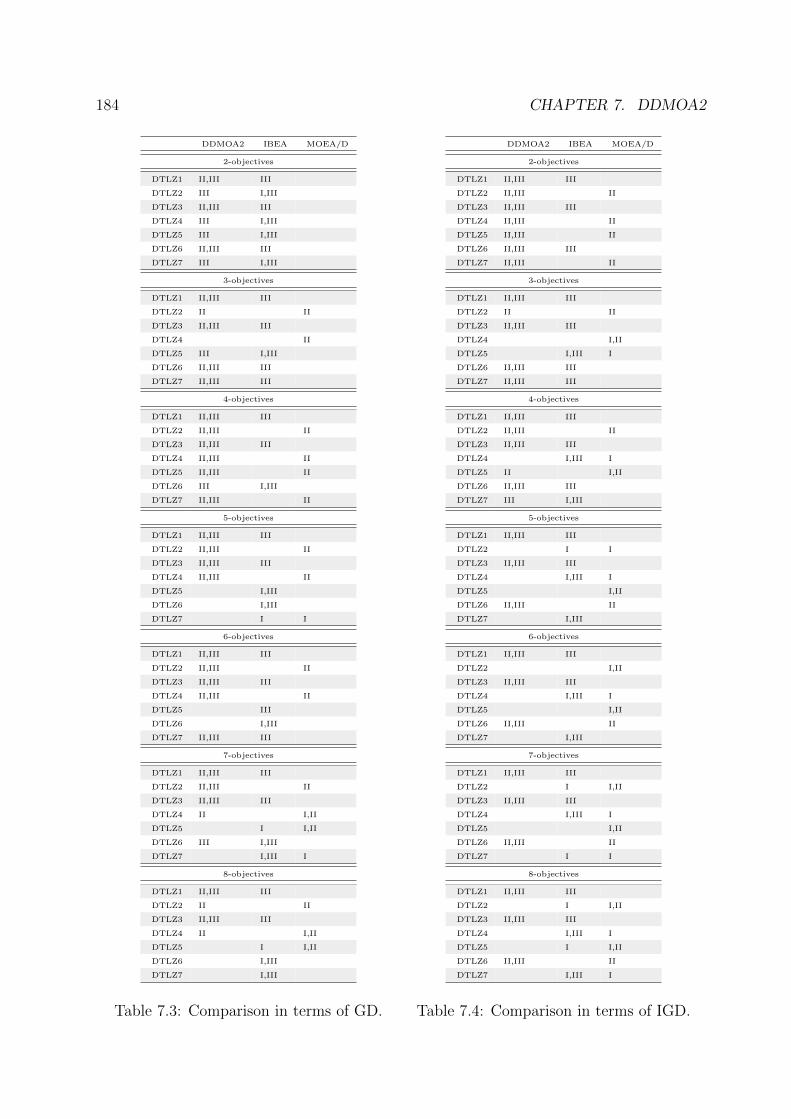
184 CHAPTER 7. DDMOA2
DDMOA2 IBEA MOEA/D
2-objectives
DTLZ1 II,III III
DTLZ2 III I,III
DTLZ3 II,III III
DTLZ4 III I,III
DTLZ5 III I,III
DTLZ6 II,III III
DTLZ7 III I,III
3-objectives
DTLZ1 II,III III
DTLZ2 II II
DTLZ3 II,III III
DTLZ4 II
DTLZ5 III I,III
DTLZ6 II,III III
DTLZ7 II,III III
4-objectives
DTLZ1 II,III III
DTLZ2 II,III II
DTLZ3 II,III III
DTLZ4 II,III II
DTLZ5 II,III II
DTLZ6 III I,III
DTLZ7 II,III II
5-objectives
DTLZ1 II,III III
DTLZ2 II,III II
DTLZ3 II,III III
DTLZ4 II,III II
DTLZ5 I,III
DTLZ6 I,III
DTLZ7 I I
6-objectives
DTLZ1 II,III III
DTLZ2 II,III II
DTLZ3 II,III III
DTLZ4 II,III II
DTLZ5 III
DTLZ6 I,III
DTLZ7 II,III III
7-objectives
DTLZ1 II,III III
DTLZ2 II,III II
DTLZ3 II,III III
DTLZ4 II I,II
DTLZ5 I I,II
DTLZ6 III I,III
DTLZ7 I,III I
8-objectives
DTLZ1 II,III III
DTLZ2 II II
DTLZ3 II,III III
DTLZ4 II I,II
DTLZ5 I I,II
DTLZ6 I,III
DTLZ7 I,III
Table 7.3: Comparison in terms of GD.
DDMOA2 IBEA MOEA/D
2-objectives
DTLZ1 II,III III
DTLZ2 II,III II
DTLZ3 II,III III
DTLZ4 II,III II
DTLZ5 II,III II
DTLZ6 II,III III
DTLZ7 II,III II
3-objectives
DTLZ1 II,III III
DTLZ2 II II
DTLZ3 II,III III
DTLZ4 I,II
DTLZ5 I,III I
DTLZ6 II,III III
DTLZ7 II,III III
4-objectives
DTLZ1 II,III III
DTLZ2 II,III II
DTLZ3 II,III III
DTLZ4 I,III I
DTLZ5 II I,II
DTLZ6 II,III III
DTLZ7 III I,III
5-objectives
DTLZ1 II,III III
DTLZ2 I I
DTLZ3 II,III III
DTLZ4 I,III I
DTLZ5 I,II
DTLZ6 II,III II
DTLZ7 I,III
6-objectives
DTLZ1 II,III III
DTLZ2 I,II
DTLZ3 II,III III
DTLZ4 I,III I
DTLZ5 I,II
DTLZ6 II,III II
DTLZ7 I,III
7-objectives
DTLZ1 II,III III
DTLZ2 I I,II
DTLZ3 II,III III
DTLZ4 I,III I
DTLZ5 I,II
DTLZ6 II,III II
DTLZ7 I I
8-objectives
DTLZ1 II,III III
DTLZ2 I I,II
DTLZ3 II,III III
DTLZ4 I,III I
DTLZ5 I I,II
DTLZ6 II,III II
DTLZ7 I,III I
Table 7.4: Comparison in terms of IGD.
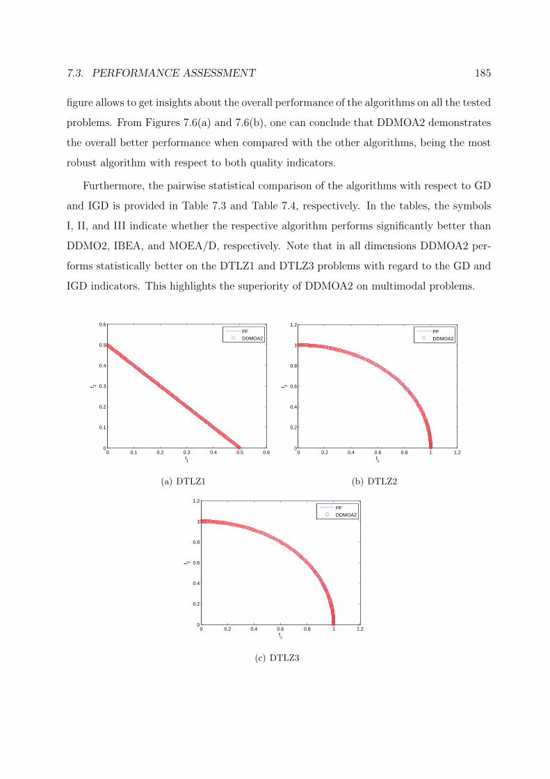
7.3. PERFORMANCE ASSESSMENT 185
figure allows to get insights about the overall performance of the algorithms on all the tested
problems. From Figures 7.6(a) and 7.6(b), one can conclude that DDMOA2 demonstrates
the overall better performance when compared with the other algorithms, being the most
robust algorithm with respect to both quality indicators.
Furthermore, the pairwise statistical comparison of the algorithms with respect to GD
and IGD is provided in Table 7.3 and Table 7.4, respectively. In the tables, the symbols
I, II, and III indicate whether the respective algorithm performs significantly better than
DDMO2, IBEA, and MOEA/D, respectively. Note that in all dimensions DDMOA2 per-
forms statistically better on the DTLZ1 and DTLZ3 problems with regard to the GD and
IGD indicators. This highlights the superiority of DDMOA2 on multimodal problems.
0 0.1 0.2 0.3 0.4 0.5 0.60
0.1
0.2
0.3
0.4
0.5
0.6
f1
f 2
PFDDMOA2
(a) DTLZ1
0 0.2 0.4 0.6 0.8 1 1.20
0.2
0.4
0.6
0.8
1
1.2
f1
f 2
PFDDMOA2
(b) DTLZ2
0 0.2 0.4 0.6 0.8 1 1.20
0.2
0.4
0.6
0.8
1
1.2
f1
f 2
PFDDMOA2
(c) DTLZ3
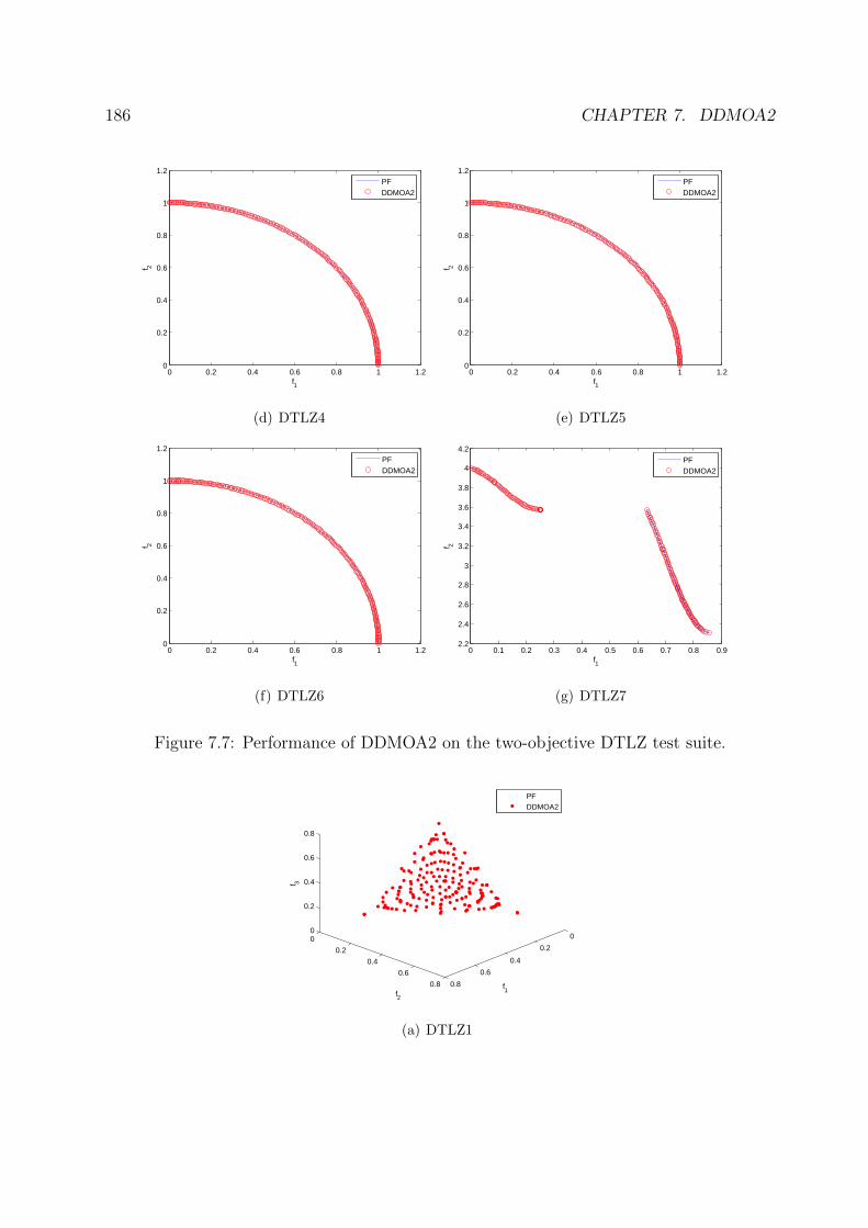
186 CHAPTER 7. DDMOA2
0 0.2 0.4 0.6 0.8 1 1.20
0.2
0.4
0.6
0.8
1
1.2
f1
f 2
PFDDMOA2
(d) DTLZ4
0 0.2 0.4 0.6 0.8 1 1.20
0.2
0.4
0.6
0.8
1
1.2
f1
f 2
PFDDMOA2
(e) DTLZ5
0 0.2 0.4 0.6 0.8 1 1.20
0.2
0.4
0.6
0.8
1
1.2
f1
f 2
PFDDMOA2
(f) DTLZ6
0 0.1 0.2 0.3 0.4 0.5 0.6 0.7 0.8 0.92.2
2.4
2.6
2.8
3
3.2
3.4
3.6
3.8
4
4.2
f1
f 2
PFDDMOA2
(g) DTLZ7
Figure 7.7: Performance of DDMOA2 on the two-objective DTLZ test suite.
0
0.2
0.4
0.6
0.8
0
0.2
0.4
0.6
0.8
0
0.2
0.4
0.6
0.8
f1f2
f 3
PFDDMOA2
(a) DTLZ1
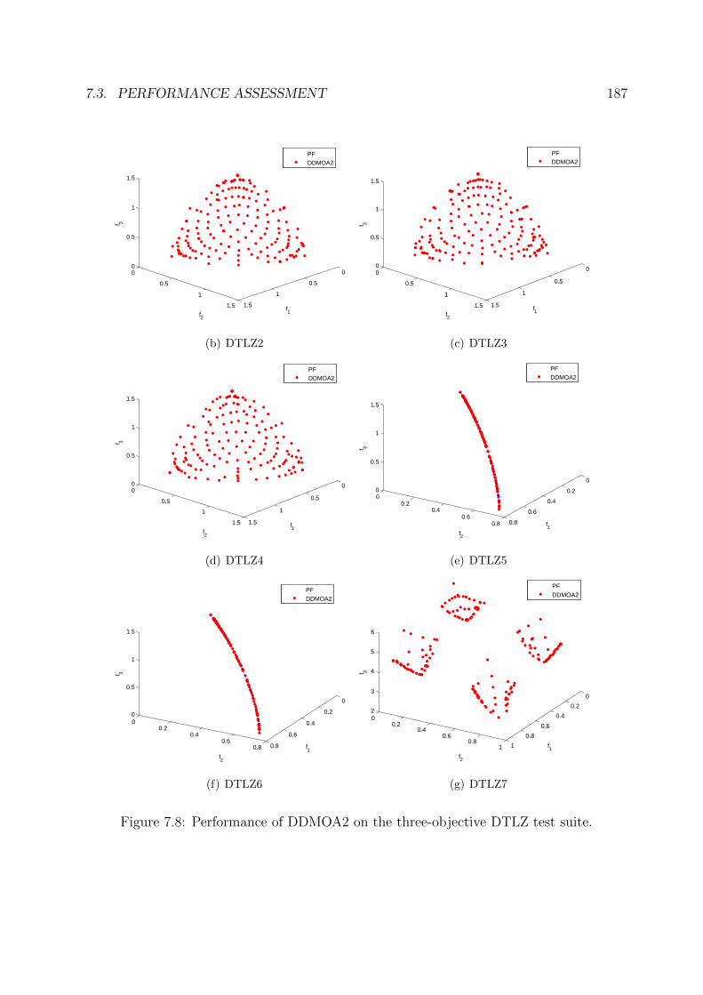
7.3. PERFORMANCE ASSESSMENT 187
0
0.5
1
1.5
0
0.5
1
1.5
0
0.5
1
1.5
f1f2
f 3
PFDDMOA2
(b) DTLZ2
0
0.5
1
1.5
0
0.5
1
1.5
0
0.5
1
1.5
f1f2
f 3
PFDDMOA2
(c) DTLZ3
0
0.5
1
1.5
0
0.5
1
1.5
0
0.5
1
1.5
f1f2
f 3
PFDDMOA2
(d) DTLZ4
0
0.2
0.4
0.6
0.8
00.2
0.40.6
0.8
0
0.5
1
1.5
f1f2
f 3PFDDMOA2
(e) DTLZ5
0
0.2
0.4
0.6
0.8
00.2
0.40.6
0.8
0
0.5
1
1.5
f1f2
f 3
PFDDMOA2
(f) DTLZ6
0
0.2
0.4
0.6
0.8
1
00.2
0.40.6
0.81
2
3
4
5
6
f1f2
f 3
PFDDMOA2
(g) DTLZ7
Figure 7.8: Performance of DDMOA2 on the three-objective DTLZ test suite.

188 CHAPTER 7. DDMOA2
Additionally, approximation sets with the best values of IGD obtained on the two and
three-objective test problems are shown in Figures 7.7 and 7.8. From the presented plots
it can be seen that DDMOA2 is able to converge and provide an adequate distribution of
solutions along the Pareto front for all the two and three-objective DTLZ test problems.
To emphasize the difference between DDMOA and DDMOA2, the IGD indicator values
obtained by both algorithms on multimodal DTLZ1 and DTLZ3 with two and three ob-
jectives are shown in Figure 7.9. From plots presented in this figure, a drastic performance
improvement can be readily observed. Although DDMOA is able to obtain comparable
indicator values on these problems, the variability of the distributions of these values are
0
1
2
3
4
5
6
7
DDMOA DDMOA2
IGD
(a) two-objective DTLZ1
0
5
10
15
20
25
DDMOA DDMOA2
IGD
(b) two-objective DTLZ3
0
1
2
3
4
5
6
DDMOA DDMOA2
IGD
(c) three-objective DTLZ1
0
5
10
15
20
25
DDMOA DDMOA2
IGD
(d) three-objective DTLZ3
Figure 7.9: Performance analysis of DDMOA and DDMOA2.

7.4. SUMMARY 189
completely different. Although in some cases it may be interesting to compare the best
indicator values, here this comparison is not carried out, as performance based on extreme
values should be read with care, if not at all avoided [33]. Here the main focus is on the
variability of the two distributions. As for real world problems, especially with compu-
tationally expensive functions, it is more important to have an algorithm that exhibits
a higher average performance and small variability, than an algorithm which converges
occasionally to the optimal region. From this perspective, it is clear that DDMOA2 is
superior compared to its predecessor. The high improvement in the variability observed in
the above plots is achieved by more extensive exploration of the search space performed
by DDMOA2. In DDMOA2, this exploration is due to the fact that all individuals in the
current population can produce offspring.
7.4 Summary
This chapter presents a generalized descent directions-guided multiobjective algorithm
(DDMOA2), which is developed on the basis of its predecessor DDMOA. Although
DDMOA2 inherits the basic principles of reproduction from its predecessor, it is generalized
in some ways. DDMOA2 maintains the population that can consist of nondominated as
well as dominated individuals. Each individual in the population has a chance to produce
offspring. This way, a better exploration of the search space is achieved, as individuals
being not promising at some stages of the search can significantly benefit to the search
as the evolution goes on. This feature is especially desirable for dealing with multimodal
problems. Furthermore, DDMOA2 does not rely on the Pareto dominance relation dur-
ing the selection process, instead the scalarizing fitness assignment is incorporated into the
parent and environmental selection procedures. The presence of nondominated solutions in
the population leads to the need for differentiation of individuals in the population. Thus,
in DDMOA2 the population consists of leader and non-leader individuals. The selection
of leaders is based on the scalarizing fitness assignment.
The performed experimental studies show the viability of the proposed approach.

190 CHAPTER 7. DDMOA2
DDMOA2 demonstrates a significantly superior performance compared to its predeces-
sor. This is achieved due to the introduced modifications. Moreover, DDMOA2 produces
highly competitive performance when compared with some state-of-the-art EMO algo-
rithms, even in high dimensional objective spaces. At the same time, DDMOA2 is often
able to outperform other algorithms on multimodal problems. However, the performance
deterioration is observed when the number of objectives is increased. This leaves open
questions for further research.
In conclusion, DDMOA2 appears a robust and efficient approach for solving continuous
multiobjective optimization problems, which is validated in several comparative studies
with other MOEAs on a number of test problems. Further, DDMOA2 is applied to solve
real-world optimization problems. Its hybrid reproduction operator is expected to be a
crucial feature to successfully deal with problems under consideration.

Chapter 8
Many-Objective Optimization using
Differential Evolution with Mutation
Restriction
8.1 Introduction
So far in this part of the thesis the main concern has been about developing EMO al-
gorithms with efficient reproduction operators for searching the Pareto optimal solutions.
The design of such operators especially for MO can require some adaptations of the algo-
rithmic framework. Thus, DDMOA2 differentiates the entire population into leader and
non-leader individuals. Moreover, leaders are further divided into subpopulations in order
to efficiently compute descent directions. In turn, DDMOA and MO-HGPSAL adopt ex-
isting approaches to perform the search in the objective space, taken advantage of their
hybrid operators for generating offspring. Although an efficient reproduction operator is
a crucial feature of either a single-objective or multiobjective optimization algorithm, the
presence of two search spaces in MO requires to develop proper selection mechanisms to
guide the search in the objective space. This becomes especially relevant to many-objective
problems.
191
192 CHAPTER 8. MYO USING DEMR
This chapter addresses the issue of fitness assignment and how to guide the search
in a high-dimensional objective space. Two different selection procedures based on the
nondominated sorting with IGD-based and clustering-based second sorting criteria are
suggested. On the other hand, a strategy to control the mutation strength in a DE operator
is proposed to handle efficiently multimodal problems.
8.2 DEMR for Multiobjective Optimization
8.2.1 NSDEMR
As it has already been stressed in this thesis, a multiobjective optimization problem inher-
its all properties of its single objectives. Differential evolution generates new individuals by
using differences of randomly sampled pairs of individuals in the current population. This
reproduction strategy allows the population to adapt to the fitness landscape of a given
problem, and makes DE invariant under any rotations of the search space. This feature
makes DE an attractive choice to solve continuous real-world optimization problems. How-
ever, DE often faces difficulties in solving multimodal problems. So this section addresses
the issue of the convergence properties of DE on multiobjective optimization problems with
a multimodal fitness landscape. A variant of a nondominated sorting differential evolution
(NSDE) [96] is considered. The outline of NSDE is given by Algorithm 13.
The algorithm works as follows. First, an initial population is randomly generated.
Next, for the predefined number of generations the evolutionary process is performed. In
each generation, each individual in the population generates one offspring employing a DE
operator (lines 9-18).
For each individual in the population, two different population members (r1 and r2)
are selected. The difference vector v is calculated using the selected individuals. In the
following, this vector is also referred as a mutation vector. Then, in order to introduce some
variation to the difference vector, it is mutated using polynomial mutation with probability
pm = 1/n, where n is the dimensionality of the decision space. Thereafter, the resulting

8.2. DEMR FOR MULTIOBJECTIVE OPTIMIZATION 193
Algorithm 13 NSDE
1: initialize: P ;
2: repeat
3: P ′ ← P , P ′′ ← ;
4: for i = 1 to µ do
5: randomly select two indexes r1 6= r2 6= i;
6: v ← xr1 − xr2
;
7: apply polynomial mutation on v;
8: restrict vector v;
9: for j = 1 to n do
10: if rand < CR then
11: yj ← xij + vj ;
12: else
13: yj ← xij ;
14: end if
15: end for
16: if xi = y then go to 10;
17: else P ′′ ← P ′′ ∪ y;
18: end if
19: end for
20: P ← environmentalSelection (P ′ ∪ P ′′);
21: until the stopping criterion is met
22: output: P ;
difference vector is restricted (line 8) and is used to mutate the corresponding parent with
probability CR.
The (If) statement in (line 16) is used to guarantee that at least one gene of the parent
individual is mutated. Some preliminary experiments showed that this approach works
better than the commonly used strategy in DE, where an integer jr is first generated and
then the jr-th gene is mutated. Used reproduction operator is similar to the
194 CHAPTER 8. MYO USING DEMR
DE/current-to-rand/1/bin variant withK = 0. If some genes of a newly generated offspring
are out of the bounds of the variables of the problem, then the corresponding lower or upper
values are assigned to these genes.
After generating the offspring population P ′′, this population is evaluated and com-
bined with the parent population P ′. Thereafter, environmentalSelection procedure is
performed in order to create a new population. This procedure is the same as the one used
in NSGA-II [46].
In the following, two different schemes to restrict the mutation vector and their impacts
on the performance of the algorithm are investigated. Generally, EAs use some sort of step
size adaptation scheme or restriction rule in order to control the mutation strength during
the search. For instance, evolution strategies use 1/5th success rule [15] or cumulative step-
size adaptation [80] for controlling the mutation strength. On the other hand, a variable-
wise restriction mechanism was proposed to control the speed of particles in SMPSO [135].
In turn, in DE the difference vector is usually scaled by multiplying it by the parameter F ,
which is a constant or may be adapted during the search. This simple strategy to control
the mutation strength may not be suitable for multimodal problems. The population can
rapidly loss diversity and, as a result, get stuck in suboptimal regions.
The following two restriction mechanisms are considered:
1. The most commonly used strategy in DE, where difference vector v is scaled by
multiplying it by the parameter F = 0.5.
2. The proposed strategy, where difference vector v is restricted as:
vj =
−δj if vj < −δjδj if vj > δj
vj otherwise
(8.2.1)
where
δj =uj − lj
2j ∈ 1, . . . , n, (8.2.2)
uj and lj are the upper and lower bounds of the j-th variable, respectively.

8.2. DEMR FOR MULTIOBJECTIVE OPTIMIZATION 195
It should be noted that the proposed restriction mechanism is the same as the one
used in SMPSO [135] to control the speed of particles. Due to some similarities in the
working principles of PSO and DE, this approach is used in the context of DE optimization.
Differential evolution with the mutation restriction mechanism shown in (8.2.2) will be
referred as DEMR. This mechanism is expected to improve the convergence properties of
DE-based algorithms on multimodal problems.
8.2.2 Performance Assessment
In the following, two variants of NSDE are under consideration: (i) uses the conventional
DE mutation restriction strategy, where mutation vector v is multiplied by parameter F ,
referred as NSDE; (ii) employs the proposed variable-wise mutation restriction (8.2.2),
referred as NSDEMR.
Experimental Setup
For each variant, 30 independent runs are performed on the ZDT4 and two-objective
DTLZ1 test problems with 30 decision variables. Both problems are highly multimodal.
For both approaches, the population size is set to 300, and the total number of generations
is 300. The remaining parameters are: the crossover probability CR = 0.15, and the
distribution index for polynomial mutation ηm = 20.
Experimental Results
To illustrate the effect of the proposed mutation restriction mechanism, Figure 8.1 shows
the length of mutation vector for randomly chosen parent in each generation. The two
plots presented in this figure refer to the medians over 30 runs. From Figure 8.1(a), one
can observe that the norm of mutation vector is larger in NSDEMR. The norms in both
algorithms become equal only at the end of the evolutionary process. From Figure 8.1(b),
it can be seen that in early generations the norm of v in NSDEMR is significantly larger.
The norms in both algorithms become to have a comparable length after 100 generations.

196 CHAPTER 8. MYO USING DEMR
0 50 100 150 200 250 3000
2
4
6
8
10
12
14
16
18
20
generation
|| V
||2
NSDENSDEMR
(a) ZDT4
0 50 100 150 200 250 3000
0.5
1
1.5
2
2.5
generation
|| V
||2
NSDENSDEMR
(b) DTLZ1
Figure 8.1: Length of mutation vector during the generations.
From the considered figures, it becomes clear that the proposed scheme to restrict
the mutation vector results in higher lengths of mutation vectors over the generations.
On the other hand, the components of mutation vector cannot be larger than the limits
imposed by the restriction mechanism. This prevents high mutations of genes to take place
during one generation. Next, the impact of increasing the length of mutation vector on the
performance of the algorithm needs to be investigated. This impact can be readily observed
0 50 100 150 200 250 3000
50
100
150
200
250
300
350
400
generation
IGD
NSDENSDEMR
(a) ZDT4
0 50 100 150 200 250 3000
100
200
300
400
500
600
700
800
900
generation
IGD
NSDENSDEMR
(b) DTLZ1
Figure 8.2: Evolution of IGD during the generations.

8.2. DEMR FOR MULTIOBJECTIVE OPTIMIZATION 197
0
5
10
15
20
NSDE NSDEMR
IGD
(a) ZDT4
0
10
20
30
40
50
60
NSDE NSDEMR
IGD
(b) DTLZ1
Figure 8.3: Comparison of NSDE and NSDEMR in terms of IGD.
in Figure 8.2. The plots presented in this figure show the median values of IGD over 30
runs during the generations. From both plots, it can be seen that NSDEMR demonstrates
the faster convergence rate and the better final values of IGD on both ZDT4 and DTLZ1
test problems. The improved performance is directly related to larger lengths of mutation
vectors in NSDEMR, preventing the algorithm from getting stuck in suboptimal regions
of the search space.
Additionally, Figure 8.3 presents the distributions of IGD produced by both algorithms
on the ZDT4 and DTLZ1 test problems. The two plots depicted in this figure clearly
highlight the superiority of NSDEMR on both problems.
8.2.3 Intermediate Summary
This section discusses a restriction mechanism to control the mutation strength in the DE-
based reproduction operator. The proposed strategy is implemented within the modified
nondominated sorting differential evolution. The effect of using the proposed mutation
restriction is studied on the multimodal ZDT4 and DTLZ1 test problems. The proposed
mechanism to control mutation strength by means of imposing the lower and upper param-
eter values on the genes of mutation vector results in higher lengths of mutation vectors

198 CHAPTER 8. MYO USING DEMR
during the evolution. Experimental results reveal that larger lengths of mutation vectors
help to prevent the population from getting stuck in locally optimal regions. Although
this section does not report on the performance of the algorithm without any restriction
mechanism (i.e. the mutation vector is not restricted at all), preliminary results showed
that this strategy performs poorly on the considered problems. In summary, the performed
experiments demonstrate a significant improvement in terms of convergence and the supe-
riority of the proposed restriction mechanism on multimodal problems. In the subsequent
sections, the variation operator based on differential evolution with mutation restriction is
used to develop efficient evolutionary many-objective optimization (EMyO) algorithms.
8.3 IGD-Based Selection for Evolutionary
Many-Objective Optimization
8.3.1 EMyO-IGD
This section presents an evolutionary many-objective optimization algorithm with
IGD-based selection (EMyO-IGD). The outline of EMyO-IGD is given by Algorithm 14.
EMyO-IGD adopts the same algorithmic framework and variation operator as used in
NSDEMR. However, the significant difference between the two algorithms lies in
environmentalSelection procedure. The selection process relies on two sorting crite-
Algorithm 14 EMyO-IGD
1: initialize: P and P ∗;
2: repeat
3: P ′ ← P , P ′′ ← ;
4: P ′′ ← variation(P ′);
5: P ← environmentalSelection(P ′ ∪ P ′′);
6: until the stopping criterion is met
7: output: P ;

8.3. IGD-BASED SELECTION FOR EMYO 199
ria: (i) nondominated sorting, and (ii) distance metric. As it is discussed in this thesis,
to successfully handle many-objective optimization problems, a proper secondary sorting
criterion must be used. Actually, there is a trend in EMO community to use quality indi-
cators in the selection process to guide the search in a high dimensional objective space.
Following this current trend, a new selection mechanism based on the IGD indicator is
developed. However, a reference set is required to calculate IGD. Thus, a set of evenly
distributed points on an (m − 1)-dimensional unit hyperplane must be provided before
the search. In Algorithm 14, this hyperplane is denoted as P ∗. In each generation, the
hyperplane is used to approximate the Pareto front for calculating IGD.
Thus, in detail environmentalSelection procedure works as follows. First, the com-
bined population P ′ ∪ P ′′ is sorted according to different non-domination levels (F1, F2
and so on). Then, each non-domination level is selected one at a time, starting from F1,
until no further level can be included without increasing the population size. Say the last
accepted non-domination level is the l-th level. In general, the last accepted level cannot be
completely accommodated. In such a case, only those solutions are kept, which maximize
the second sorting criterion.
As the second sorting criterion, a distance metric based on the inverted generational
distance is used. For choosing the remaining k = |P |−∑l−1
i=1 |Fi| population members from
the last accepted front Fl, the following steps are performed:
1. The objectives of the solutions in Fl are normalized as:
f i =fi − fmin
i
fmaxi − fmin
i
, ∀i ∈ 1, . . . ,m (8.3.1)
where fmini and fmax
i are the minimum and maximum values of the i-th objective in
Fl, respectively. f i ∈ [0, 1],∀i ∈ 1, . . . ,m is the normalized objective value.
2. If there are normalized solutions in Fl that are below the unit hyperplane, then the
hyperplane is moved until no solutions are below it. The resulting hyperplane is used
as a reference set to calculate IGD for the normalized set of objective vectors in Fl.
200 CHAPTER 8. MYO USING DEMR
3. For each a ∈ Fl, a distance metric I[a] based on IGD is calculated as:
I[a] = IGD(P ∗, A) (8.3.2)
where A = Fl\a, and P ∗ is the reference set.
In (8.3.2), the quality of solution a is evaluated by calculating the IGD metric of the
set Fl without the solution a. The metric is the resulting IGD for the set Fl removing a.
The higher value of I[a], the better quality of solution a is, as removing solution a leads to
a higher value of IGD that, in turn, corresponds to a poorer performance of the resulting
set. Thus, removing the solutions with high values of I[a] is undesirable, so they should
be kept in the population.
Therefore, after computing the distance metric I for each solution in Fl, the set Fl is
sorted in descending order with respect to I. Finally, k first elements of the sorting set are
included into P .
8.3.2 Performance Assessment
In the following, EMyO-IGD is compared with IBEA [198], GDE3 [116], SMPSO [135],
and MOEA/D [123]. The main concern of the study is the ability of the algorithms to
guide the search in a high dimensional objective space. Although SMPSO and GDE3
are expected to perform poorly when the number of objectives is increased, they serve as
an important reference as they are state-of-the-art EMO algorithms. Moreover, it is also
interesting to compare the convergence property of stochastic direct search algorithms on
multimodal problems, thereby validating the proposed mutation restriction mechanism.
The DTLZ test suite is used as the basis for comparison, since it can be scaled to an
arbitrary number of objectives. Thus, the DTLZ1-4 test problems are adopted, each with
30 decision variables, ranging from 2 to 20 objectives.

8.3. IGD-BASED SELECTION FOR EMYO 201
EMyO-IGD MOEA/D IBEA SMPSO GDE3
CR = 0.15 CR = 0.15 pc = 0.9 ηm = 20 CR = 0.15
ηm = 20 F = 0.5 ηc = 20 pm = 1/n F = 0.5
pm = 1/n ηm = 20 ηm = 20
|P ∗| = 500 pm = 1/n pm = 1/n
Table 8.1: Parameter settings for the algorithms.
Experimental Setup
EMyO-IGD and MOEA/D are implemented in the MATLAB R© programming language,
IBEA is used within the PISA framework [16], whereas GDE3 and SMPSO are provided
by the jMetal framework [62]. For each algorithm, 30 independent runs are performed
on each problem with a population size of µ = 300, running for 500 generations. The
remaining parameter settings for the algorithms are presented in Table 8.1 (the parameters
not specified use the default values as stated in the corresponding papers).
Experimental Results
Figure 8.4 presents the graphical representation of the median values of the hypervolume
indicator and IGD obtained by all the algorithms on the benchmark functions with varying
dimensions.
Problems DTLZ1,3 are known to be hard to solve as they contain a very large number of
local Pareto optimal fronts [50], so they are considered in more detail. For DTLZ1, EMyO-
IGD achieves the best hypervolume for m > 2, except for m = 20, where the best median
hypervolume is obtained by MOEA/D. However, in terms of the IGD indicator EMyO-
IGD provides better results for m > 2 than the other four algorithms on DTLZ1. For
DTLZ3, EMyO-IGD achieves the best hypervolume for 2 < m < 15. Similar performance
is observed in terms of the IGD indicator.
Concerning the other problems, EMyO-IGD is always better, concerning both quality
indicators, than SMPSO and GDE3 for m > 3, except for DTLZ4 with five objectives,
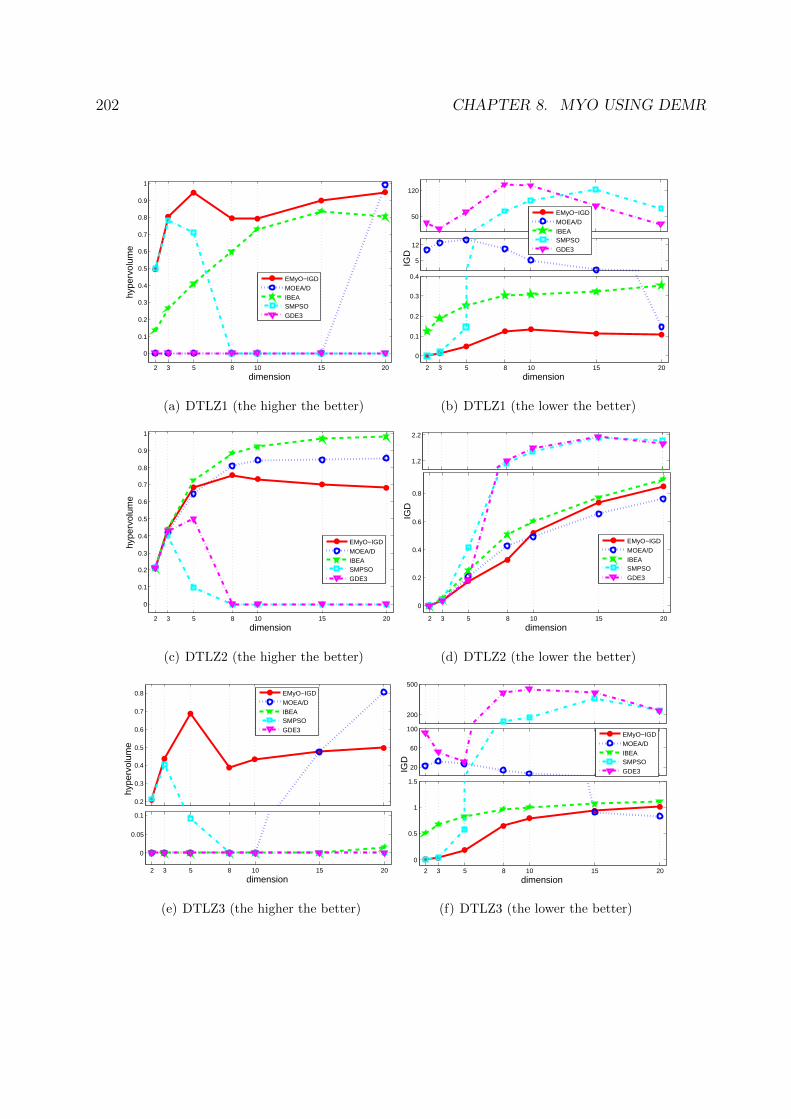
202 CHAPTER 8. MYO USING DEMR
2 3 5 8 10 15 20
0
0.1
0.2
0.3
0.4
0.5
0.6
0.7
0.8
0.9
1
dimension
hype
rvol
ume
EMyO−IGDMOEA/DIBEASMPSOGDE3
(a) DTLZ1 (the higher the better)
50
120
2 3 5 8 10 15 20
0
0.1
0.2
0.3
0.4
dimension
5
12
IGD
EMyO−IGDMOEA/DIBEASMPSOGDE3
(b) DTLZ1 (the lower the better)
2 3 5 8 10 15 20
0
0.1
0.2
0.3
0.4
0.5
0.6
0.7
0.8
0.9
1
dimension
hype
rvol
ume
EMyO−IGDMOEA/DIBEASMPSOGDE3
(c) DTLZ2 (the higher the better)
2 3 5 8 10 15 20
0
0.2
0.4
0.6
0.8
dimension
IGD
1.2
2.2
EMyO−IGDMOEA/DIBEASMPSOGDE3
(d) DTLZ2 (the lower the better)
0.2
0.3
0.4
0.5
0.6
0.7
0.8
hype
rvol
ume
2 3 5 8 10 15 20
0
0.05
0.1
dimension
EMyO−IGDMOEA/DIBEASMPSOGDE3
(e) DTLZ3 (the higher the better)
200
500
2 3 5 8 10 15 20
0
0.5
1
1.5
dimension
20
60
100
IGD
EMyO−IGDMOEA/DIBEASMPSOGDE3
(f) DTLZ3 (the lower the better)

8.3. IGD-BASED SELECTION FOR EMYO 203
0.2
0.3
0.4
0.5
0.6
0.7
hype
rvol
ume
0.8
0.9
1
2 3 5 8 10 15 20
0
0.1
dimension
EMyO−IGDMOEA/DIBEASMPSOGDE3
(g) DTLZ4 (the higher the better)
1
1.5
2 3 5 8 10 15 200
0.1
0.2
0.3
0.4
0.5
dimension
0.6
0.7
0.8
IGD
EMyO−IGDMOEA/DIBEASMPSOGDE3
(h) DTLZ4 (the lower the better)
Figure 8.4: Performance comparison of EMyO-IGD, MOEA/D, IBEA, SMPSO, and GDE3
on the DTLZ1-4 test problems. The plots present the median values of the hypervolume
(left hand side) and IGD (right hand side) over 30 runs.
where GDE3 yields the best results among all the algorithms in terms of IGD. Moreover,
EMyO-IGD is always better than IBEA with respect to IGD, except for DTLZ4 with
m = 2. Furthermore, IBEA provides the best hypervolume among all algorithms for m > 2
on DTLZ2 and DTLZ4. However, these problems do not present as much difficulties in
terms of convergence to the Pareto front as the other considered problems, and IBEA is
the only considered indicator based algorithm (the epsilon indicator was used) while the
other algorithms use a diversity mechanism which attempts to uniformly distribute points
along the Pareto front.
From the above discussion, it can be seen that EMyO-IGD performs the best on the
multimodal problems (DTLZ1 and DTLZ3). Better results are only obtained by SMPSO
for m = 2, which also outperforms all the algorithms in terms of IGD on all the problems
with two objectives. MOEA/D performs better with regard to the hypervolume than
EMyO-IGD on DTLZ1 with m = 20, and in terms of IGD on DTLZ3 with m = 20.
EMyO-IGD is the only algorithm which is able to converge to the Pareto front for
all the problems, providing an adequate distribution of solutions along the Pareto front.
Although IBEA converges to the Pareto front for all the problems too, it is observed

204 CHAPTER 8. MYO USING DEMR
0 0.1 0.2 0.3 0.4 0.5 0.60
0.1
0.2
0.3
0.4
0.5
0.6
f1
f 2
(a) two-objective DTLZ1
0 0.1 0.2 0.3 0.4 0.5 0.60
0.1
0.2
0.3
0.4
0.5
0.6
f1
f 2
(b) two-objective DTLZ1
0 0.1 0.2 0.3 0.4 0.5 0.60
0.1
0.2
0.3
0.4
0.5
0.6
f1
f 2
(c) two-objective DTLZ1
00.2
0.40.6
0.8
00.2
0.40.6
0.8
0
0.2
0.4
0.6
0.8
f1f2
f 3
(d) three-objective DTLZ1
00.2
0.4
0.60.8
0
0.2
0.4
0.6
0.8
0
0.2
0.4
0.6
0.8
f1f2
f 3
(e) three-objective DTLZ1
00.2
0.40.6
0.8
00.2
0.40.6
0.8
0
0.2
0.4
0.6
0.8
f1f2
f 3
(f) three-objective DTLZ1
0 0.2 0.4 0.6 0.8 1 1.20
0.2
0.4
0.6
0.8
1
1.2
f1
f 2
(g) two-objective DTLZ3
0 0.2 0.4 0.6 0.8 1 1.20
0.2
0.4
0.6
0.8
1
1.2
f1
f 2
(h) two-objective DTLZ3
0 0.2 0.4 0.6 0.8 1 1.20
0.2
0.4
0.6
0.8
1
1.2
f1
f 2
(i) two-objective DTLZ3
00.5
11.5
00.5
11.5
0
0.5
1
1.5
f1f2
f 3
(j) three-objective DTLZ3
0
0.5
1
1.5
0
0.5
1
1.5
0
0.5
1
1.5
f1f2
f 3
(k) three-objective DTLZ3
0
0.5
1
1.5
0
0.5
1
1.5
0
0.5
1
1.5
f1f2
f 3
(l) three-objective DTLZ3
Figure 8.5: Performance of EMyO-IGD (left), IBEA (middle), SMPSO (right) on the two
and three-objective DTLZ1 and DTLZ3 test problems.

8.3. IGD-BASED SELECTION FOR EMYO 205
that it is able to converge only to the corner points of the Pareto front for DTLZ1 and
DTLZ3. Figure 8.5 displays approximation sets with the best values of IGD obtained
on the multimodal DTLZ1 and DTLZ3 test problems. The figure does not present the
performance of the algorithms that did not converge to the Pareto front for these problems.
A good convergence of EMyO-IGD on multimodal problems is due to the proposed
restriction mechanism used in the DE reproduction operator. EMyO-IGD clearly out-
performs all of the considered DE-based algorithms on multimodal problems, even in
low-dimensional objective spaces where the selection mechanism of all the algorithms is
expected to work well.
However, it is interesting to note that with the increasing number of objectives the
performance of MOEA/D becomes notably better in terms of both quality indicators, es-
pecially on multimodal problems. Such behavior is related to the properties of the DTLZ
test suite. The decision space of multiobjective problems consists of k position- and l
distance-related parameters (n = k + l) [87]. For the DTLZ test suite, the number of
position-related parameters is k = m − 1, and the number of distance-related parameters
which account for the convergence is l = n − m + 1. Thus, when the number of objec-
tives increases and the total number of decision variables remains constant, the number of
distance-related parameters decreases. Such situation results in that a problem in question
has a lower number of local Pareto fronts, consequently it is much easier to converge to
the Pareto front.
Such scenario can be easily observed in the case of DTLZ1. In Figures 8.4(a) and 8.4(b),
one can see that if m ≤ 15, the number of distance-related parameters is l = n−m+1 ≥ 16,
MOEA/D is unable to converge that results in zero hypervolume and high values of IGD.
However, if m = 20 then l = 11, and MOEA/D succeeds to converge to the Pareto
front. Nevertheless, when the number of distance-related parameters is high, especially
in the case of two and three dimensions, EMyO-IGD is the only among all of the tested
DE-based algorithms that converges to the Pareto front. At the same time, EMyO-IGD
provides highly competitive results compared to SMPSO on multimodal benchmarks with
two and three objectives (Figure 8.5).

206 CHAPTER 8. MYO USING DEMR
EMyO-IGD MOEA/D IBEA SMPSO GDE3
2-objectives
DTLZ1 II,III,V II,V I,II,III,V
DTLZ2 I,III I I,II,III I,II,III,IV
DTLZ3 II,III,V I,II,III,V
DTLZ4 I,III I I,II,III I,II,III,IV
3-objectives
DTLZ1 II,III,IV,V II,V II,III,V
DTLZ2 II,IV,V IV I,II,IV,V II,IV
DTLZ3 II,III,IV,V II,III,V
DTLZ4 II,IV,V IV I,II,IV,V II,IV
5-objectives
DTLZ1 II,III,IV,V II,V II,III,V
DTLZ2 II,IV,V IV,V I,II,IV,V IV
DTLZ3 II,III,IV,V II,III,V
DTLZ4 II,IV,V IV,V I,II,IV,V IV
8-objectives
DTLZ1 II,III,IV,V II,IV,V
DTLZ2 IV,V I,IV,V I,II,IV,V IV
DTLZ3 II,III,IV,V
DTLZ4 II,IV,V IV,V I,II,IV,V IV
10-objectives
DTLZ1 II,III,IV,V II,IV,V
DTLZ2 IV,V I,IV,V I,II,IV,V
DTLZ3 II,III,IV,V
DTLZ4 II,IV,V IV,V I,II,IV,V IV
15-objectives
DTLZ1 II,III,IV,V IV,V II,IV,V
DTLZ2 IV,V I,IV,V I,II,IV,V
DTLZ3 III,IV,V III,IV,V III III
DTLZ4 IV,V I,IV,V I,II,IV,V
20-objectives
DTLZ1 III,IV,V I,III,IV,V IV,V IV
DTLZ2 IV,V I,IV,V I,II,IV,V
DTLZ3 III,IV,V I,III,IV,V IV,V
DTLZ4 IV,V I,IV,V I,II,IV,V V
Table 8.2: Statistical comparison in terms of the hypervolume.

8.3. IGD-BASED SELECTION FOR EMYO 207
EMyO-IGD MOEA/D IBEA SMPSO GDE3
2-objectives
DTLZ1 II,III,V V II,V I,II,III,V
DTLZ2 III I,III I,II,III,V I,II,III
DTLZ3 II,III,V V II,V I,II,III,V
DTLZ4 I,III I I,II,III,V I,II,III
3-objectives
DTLZ1 II,III,IV,V V II,V II,III,V
DTLZ2 III,IV III,IV III I,II,III,IV
DTLZ3 II,III,V V II,V II,III,V
DTLZ4 II,III,IV III,IV III I,II,III,IV
5-objectives
DTLZ1 II,III,IV,V V II,V II,III,V
DTLZ2 II,III,IV,V III,IV IV II,III,IV
DTLZ3 II,III,IV,V V II,V II,V
DTLZ4 II,III,IV IV II,IV I,II,III,IV
8-objectives
DTLZ1 II,III,IV,V IV,V II,IV,V V
DTLZ2 II,III,IV,V III,IV,V IV,V V
DTLZ3 II,III,IV,V IV,V II,IV,V V
DTLZ4 II,III,IV,V IV,V II,IV,V IV
10-objectives
DTLZ1 II,III,IV,V IV,V II,IV,V V
DTLZ2 III,IV,V I,III,IV,V IV,V V
DTLZ3 II,III,IV,V IV,V II,IV,V V
DTLZ4 II,III,IV,V IV,V II,IV,V IV
15-objectives
DTLZ1 II,III,IV,V IV,V II,IV,V IV
DTLZ2 III,IV,V I,III,IV,V IV,V
DTLZ3 III,IV,V III,IV,V IV,V V
DTLZ4 II,III,IV,V IV,V II,IV,V IV
20-objectives
DTLZ1 II,III,IV,V III,IV,V IV,V IV
DTLZ2 III,IV,V I,III,IV,V IV,V IV
DTLZ3 III,IV,V I,III,IV,V IV,V
DTLZ4 III,IV,V III,IV,V IV,V
Table 8.3: Statistical comparison in terms of IGD.
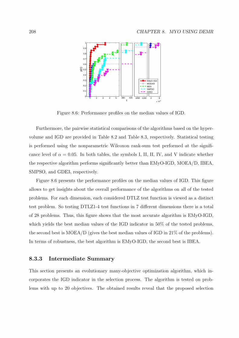
208 CHAPTER 8. MYO USING DEMR
1 2 3 4 50
0.1
0.2
0.3
0.4
0.5
0.6
0.7
0.8
0.9
1
ρ(τ)
380 420τ
1050 1150 2 8
x 104
EMyO−IGDMOEA/DIBEASMPSOGDE3
Figure 8.6: Performance profiles on the median values of IGD.
Furthermore, the pairwise statistical comparisons of the algorithms based on the hyper-
volume and IGD are provided in Table 8.2 and Table 8.3, respectively. Statistical testing
is performed using the nonparametric Wilcoxon rank-sum test performed at the signifi-
cance level of α = 0.05. In both tables, the symbols I, II, II, IV, and V indicate whether
the respective algorithm performs significantly better than EMyO-IGD, MOEA/D, IBEA,
SMPSO, and GDE3, respectively.
Figure 8.6 presents the performance profiles on the median values of IGD. This figure
allows to get insights about the overall performance of the algorithms on all of the tested
problems. For each dimension, each considered DTLZ test function is viewed as a distinct
test problem. So testing DTLZ1-4 test functions in 7 different dimensions there is a total
of 28 problems. Thus, this figure shows that the most accurate algorithm is EMyO-IGD,
which yields the best median values of the IGD indicator in 50% of the tested problems,
the second best is MOEA/D (gives the best median values of IGD in 21% of the problems).
In terms of robustness, the best algorithm is EMyO-IGD, the second best is IBEA.
8.3.3 Intermediate Summary
This section presents an evolutionary many-objective optimization algorithm, which in-
corporates the IGD indicator in the selection process. The algorithm is tested on prob-
lems with up to 20 objectives. The obtained results reveal that the proposed selection

8.4. CLUSTERING-BASED SELECTION FOR EMYO 209
scheme is able to effectively guide the search in a high-dimensional objective space. The
algorithm produces highly competitive results compared with some state-of-the-art many-
objective optimization algorithms. EMyO-IGD shows ability to produce well-covered and
well-distributed approximations to the set of Pareto optimal solutions for all the considered
problems. Therefore, it can be used as a viable alternative to solve optimization problems
with a large number of objectives.
8.4 Clustering-Based Selection for Evolutionary
Many-Objective Optimization
8.4.1 EMyO-C
The previous section introduces an approach based on the IGD indicator to handle many-
objective problems, where a reference set is used to approximate the Pareto front for calcu-
lating distance metrics for each solution in the last non-domination level. The experimental
results show that this strategy allows to effectively guide the search in a high-dimensional
objective space. The idea of using a set of evenly distributed reference points has been
adopted in some other studies [3, 44, 104]. All these proposed approaches significantly
improve the scalability of EMO algorithms and appear to be suitable for dealing with
many-objective problems. However, the major drawback of these approaches is that all of
them require the user to specify a set of evenly distributed points on the unit hyperplane.
In turn, it is not always an easy task especially for higher dimensions. Furthermore, chang-
ing the population size often requires to change the number of points on the hyperplane.
These issues make EMO algorithms less flexible and less attractive to practitioners.
This section presents an evolutionary many-objective optimization algorithm with
clustering-based selection (EMyO-C), which is developed to overcome the aforementioned
difficulties. The outline of EMyO-C is given by Algorithm 14. The only difference between
EMyO-IGD and EMyO-C is in environmentalSelection procedure. EMyO-C performs
the selection process relying on the nondominated sorting to sort the combined population

210 CHAPTER 8. MYO USING DEMR
according to different non-domination levels and a clustering-based procedure to select
individuals from the last non-domination level.
In order to select the remaining k = |P | −∑l−1
i=1 |Fi| population members from the last
accepted non-domination front Fl, the following steps are performed:
1. The distances from each individual in Fl to the reference point are calculated in the
objective space.
2. Each objective of an individual in Fl is translated by substracting objective fi by
fmini , where fmin
i is the minimum value of the i-th objective in Fl. As a result, the
ideal point of Fl is a zero vector, and objectives in Fl are nonnegative.
3. Each individual in Fl is projected on the unit hyperplane.
4. Clustering technique is performed using projected individuals in order to form k
clusters.
5. From each cluster, a representative is selected, where a cluster representative is an
individual having the smallest distance to the reference point.
Using this procedure, k individuals are selected and added to the population of the next
generation. It should be be noted that this procedure is easy to implement, and it is
completely self-adaptive.
The reference point z used in the above described procedure is initialized by setting
the minimum values of each objective in the initial population (zj = min1≤i≤µ fj(xi)). At
the end of each generation, the components of the reference point are updated if there are
smaller objective values in the offspring population. The clustering algorithm is as follows:
Step 1 Initially, each point belongs to a separate cluster (Ci = i), so that
C = C1, C2, . . . , C|Fl|.
Step 2 If |C| ≤ k, stop. Otherwise, go to Step 3.

8.4. CLUSTERING-BASED SELECTION FOR EMYO 211
Step 3 For each pair of clusters, calculate the distance between two cluster d12 as:
d12 =1
|C1||C2|∑
i∈C1,j∈C2
d(i, j),
where d(i, j) is the Euclidean distance between two points i and j. Find the pair
(i1, i2) which corresponds to the minimum cluster-distance.
Step 4 Merge the clusters Ci1 and Ci2 . This reduces the size of C by one.
Go to Step 2.
If implemented in a proper way, the complexity of the above clustering algorithm is
O(m|Fl|2) [42]. So the complexity is mainly governed by the number of points in Fl,
while it is polynomial in the number of objectives. This feature is especially attractive to
solve problems with a large number of objectives.
8.4.2 Performance Assessment
In the following, EMyO-C is compared with EMyO-IGD and IBEA. The main concern of
this study is to investigate the ability of the clustering-based selection scheme to guide
the search in a high-dimensional objective space. The performance of the algorithms is
studied on the DTLZ1-3,7 test problems with 30 decision variables. Since these problems
have different Pareto front geometries, including linear, concave, and disconnected geome-
tries, strengths and weakness of different selection schemes used by the algorithms can be
identified.
Experimental Setup
For each algorithm, 30 independent runs are performed on each problem with a population
size of 300, running for 500 generations. Further parameters for IBEA and EMyO-IGD
are the same as the ones used in the previous section. EMyO-C uses the same parameter
settings as EMyO-IGD.

212 CHAPTER 8. MYO USING DEMR
Experimental Results
Figure 8.7 shows the median values of the IGD indicator obtained by three algorithms
on the DTLZ1-3,7 test problems with varying dimensions. From Figure 8.7(a), it can
be seen that EMyO-C has the worst performance on DTLZ1 with 10 and 15 objectives.
However, in other dimensions the performance of EMyO-C is very close to that produced
by EMyO-IGD, which generally performs the best on this problem. It is not surprising,
2 3 5 10 15 20
0
0.05
0.1
0.15
0.2
0.25
0.3
0.35
0.4
0.45
0.5
dimension
IGD
IBEAEMyO−IGDEMyO−C
(a) DTLZ1 (the lower the better)
2 3 5 10 15 20
0
0.1
0.2
0.3
0.4
0.5
0.6
0.7
0.8
0.9
dimension
IGD
IBEAEMyO−IGDEMyO−C
(b) DTLZ2 (the lower the better)
2 3 5 10 15 20
0
0.2
0.4
0.6
0.8
1
1.2
1.4
dimension
IGD
IBEAEMyO−IGDEMyO−C
(c) DTLZ3 (the lower the better)
2 3 5 10 15 20
0
2
4
6
8
10
12
dimension
IGD
IBEAEMyO−IGDEMyO−C
(d) DTLZ7 (the lower the better)
Figure 8.7: Performance comparison of EMyO-C, EMyO-IGD, and IBEA on
the DTLZ1-3,7 test problems.

8.4. CLUSTERING-BASED SELECTION FOR EMYO 213
since EMyO-IGD uses unit hyperplane in its selection process, which coincides with the
Pareto front geometry of this problem. EMyO-C produces similar performance as EMyO-
IGD on DTLZ2 and DTLZ3 with up to 5 objectives (Figures 8.7(b) and 8.7(c)). Both
algorithms outperform IBEA on these two problems with respect to the IGD indicator.
However, EMyO-C performs the best on DTLZ2 and DTLZ3 when the dimensionality of
the objective space is larger than 5 (Figures 8.7(b) and 8.7(c)). In Figure 8.7(d), one can
see that EMyO-C outperforms all the other algorithms in higher dimensions on DTLZ7. It
is interesting to note that, when the number of objectives grows, the performance of EMyO-
IGD on this problem becomes increasingly poorer. This is due to the fact that the unit
hyperplane used in EMyO-IGD cannot approximate the Pareto front geometry of DTLZ7
properly. In this case, the selection mechanism used in EMyO-C becomes particularly
useful.
Furthermore, in order to show the scalability of the proposed approach, EMyO-C is run
on DTLZ2 with 50 and 100 objectives, having 60 and 110 decision variables, respectively.
Parameter settings for EMyO-C are the same as in the previous experiment. To measure
the convergence of solutions in the final population P to the Pareto front, the proximity
indicator [142] is used, which is defined as:
Ip = median
(
m∑i=1
(fi(x))2
) 12
− 1
. (8.4.1)
Smaller values of Ip indicate that the population P is closer to the Pareto optimal front.
Figure 8.8 shows the distributions of the proximity indicator for the final populations
returned by EMyO-C on the DTLZ2 test problem with 50 and 100 objectives over 30
runs. The small values of Ip presented in the plot clearly indicate that EMyO-C converges
to the Pareto front in the presence of such a large number of objectives. Moreover, the
relatively small variability of the values of Ip in both 50 and 100-dimensional objective
spaces emphasizes the robustness of the approach.
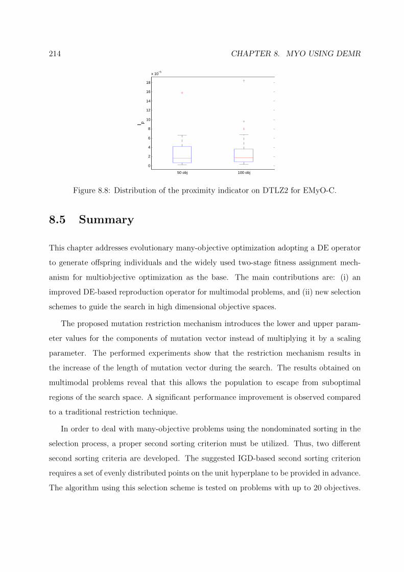
214 CHAPTER 8. MYO USING DEMR
0
2
4
6
8
10
12
14
16
18
x 10−5
50 obj 100 obj
I p
Figure 8.8: Distribution of the proximity indicator on DTLZ2 for EMyO-C.
8.5 Summary
This chapter addresses evolutionary many-objective optimization adopting a DE operator
to generate offspring individuals and the widely used two-stage fitness assignment mech-
anism for multiobjective optimization as the base. The main contributions are: (i) an
improved DE-based reproduction operator for multimodal problems, and (ii) new selection
schemes to guide the search in high dimensional objective spaces.
The proposed mutation restriction mechanism introduces the lower and upper param-
eter values for the components of mutation vector instead of multiplying it by a scaling
parameter. The performed experiments show that the restriction mechanism results in
the increase of the length of mutation vector during the search. The results obtained on
multimodal problems reveal that this allows the population to escape from suboptimal
regions of the search space. A significant performance improvement is observed compared
to a traditional restriction technique.
In order to deal with many-objective problems using the nondominated sorting in the
selection process, a proper second sorting criterion must be utilized. Thus, two different
second sorting criteria are developed. The suggested IGD-based second sorting criterion
requires a set of evenly distributed points on the unit hyperplane to be provided in advance.
The algorithm using this selection scheme is tested on problems with up to 20 objectives.

8.5. SUMMARY 215
EMyO-IGD demonstrates the ability to effectively guide the search in a high-dimensional
objective space producing highly competitive results, when compared with other state-of-
the-art many-objective algorithms. However, drawbacks due to the need to specify a set of
uniformly distributed points and relatively poor performance on problems with a complex
Pareto front geometry are identified. To overcome these drawbacks, the clustering-based
selection is suggested. The performed experiments show that this selection mechanism is
able to guide the search in a high-dimensional objective space. Although some limitations
of the IGD-based selection are overcome, it is observed that EMyO-C produces sightly
poorer performance on some test instances. However, the results obtained on problems
with a large number of objectives clearly indicate a promising direction for future research.

216 CHAPTER 8. MYO USING DEMR

Part III
Applications
217


Chapter 9
Dengue Disease Transmission
During the last decades, the global prevalence of dengue progressed dramatically. It is
a disease which is now endemic in more than one hundred countries of Africa, America,
Asia, and the Western Pacific. This chapter presents a mathematical model for the dengue
disease transmission and uses a multiobjective approach to find an optimal strategy to
control the disease.
9.1 Disease Background
Dengue is a vector-borne disease transmitted from an infected human to a female Aedes
mosquito by a bite. Then, the mosquito, that needs regular meals of blood to feed their
eggs, bites a potentially healthy human and transmits the disease, turning it into a cycle.
There are two forms of dengue: dengue fever (DF) and dengue hemorrhagic fever
(DHF). The first one is characterized by a sudden high fever without respiratory symptoms,
accompanied by intense headaches, pain in joints and muscles and lasts between three to
seven days. Humans may only transmit the virus during the febrile stage. DHF initially
exhibits a similar, if more severe pathology as DF, but deviates from the classic pattern
at the end of the febrile stage. Additionally, the hemorrhagic form is characterized by
nose bleeding, skin or mouth and gums bruising, nausea, vomiting and fainting due to
219

220 CHAPTER 9. DENGUE DISEASE TRANSMISSION
Figure 9.1: Mosquito Aedes aegypti (adapted from [147]).
low blood pressure and fluid leakage. It usually lasts between two to three days and may
have lethal outcome. Nowadays, dengue is the mosquito-borne infection that has become
a major international public health concern. According to the World Health Organization
(WHO), 50 to 100 million dengue fever infections occur yearly, including 500000 dengue
hemorrhagic fever cases and 22000 deaths, mostly among children [186].
There are four distinct, but closely related, viruses that cause dengue. The four
serotypes, named DEN-1 to DEN-4, belong to the Flavivirus family, but they are anti-
genically distinct. Recovery from infection by one virus provides lifelong immunity against
that virus but provides only partial and transient protection against subsequent infection
by the other three viruses. There are strong evidences that a sequential infection increases
the risk of developing DHF.
The spread of dengue is attributed to the geographic expansion of the mosquitoes re-
sponsible for the disease: Aedes aegypti and Aedes albopictus. The Aedes aegypti mosquito
(Figure 9.1) is a tropical and subtropical species widely distributed around the world,
mostly between latitudes 35oN and 35oS. In urban areas, Aedes mosquitoes breed on water
collections in artificial containers such as cans, plastic cups, used tires, broken bottles and
flower pots. Due to its high interaction with humans and its urban behavior, the Aedes
aegypti mosquito is considered the major responsible for the dengue transmission.
Dengue is spread only by adult females that require blood consumption for the devel-
opment of their eggs, whereas male mosquitoes feed on fruit nectar and other sources of
sugar. In this process, the female mosquitoes acquire the virus while feeding from the blood
of an infected person. After virus incubation from eight to twelve days (extrinsic period)
and for the rest of its life, an infected mosquito is capable of transmitting the virus to
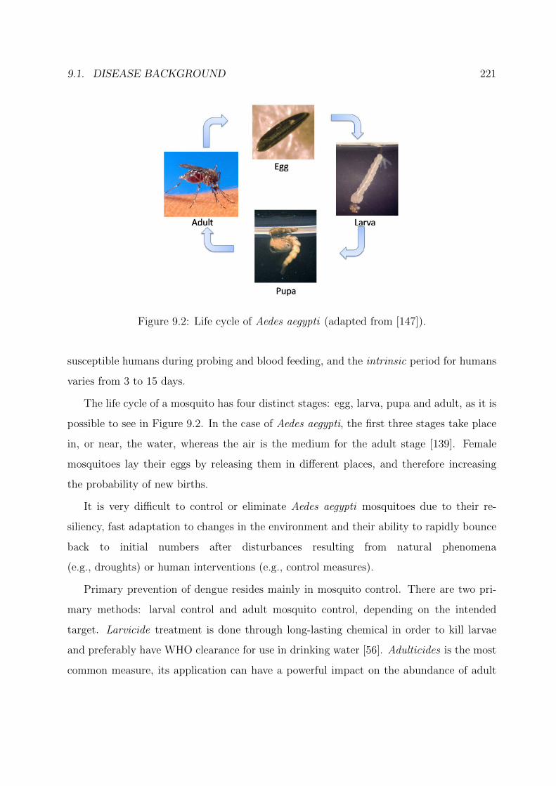
9.1. DISEASE BACKGROUND 221
Figure 9.2: Life cycle of Aedes aegypti (adapted from [147]).
susceptible humans during probing and blood feeding, and the intrinsic period for humans
varies from 3 to 15 days.
The life cycle of a mosquito has four distinct stages: egg, larva, pupa and adult, as it is
possible to see in Figure 9.2. In the case of Aedes aegypti, the first three stages take place
in, or near, the water, whereas the air is the medium for the adult stage [139]. Female
mosquitoes lay their eggs by releasing them in different places, and therefore increasing
the probability of new births.
It is very difficult to control or eliminate Aedes aegypti mosquitoes due to their re-
siliency, fast adaptation to changes in the environment and their ability to rapidly bounce
back to initial numbers after disturbances resulting from natural phenomena
(e.g., droughts) or human interventions (e.g., control measures).
Primary prevention of dengue resides mainly in mosquito control. There are two pri-
mary methods: larval control and adult mosquito control, depending on the intended
target. Larvicide treatment is done through long-lasting chemical in order to kill larvae
and preferably have WHO clearance for use in drinking water [56]. Adulticides is the most
common measure, its application can have a powerful impact on the abundance of adult

222 CHAPTER 9. DENGUE DISEASE TRANSMISSION
mosquito vector. However, the efficacy is often constrained by the difficulty in achieving
sufficiently high coverage of resting surfaces [58].
The most recent approach for fighting the disease is biological control. It is a natu-
ral process of population regulation through natural enemies. There are techniques that
combine some parasites that kill partially the larval population; however, the operational
difficulty stems from the lack of expertise in producing this type of parasites as well as
cultural objections in introducing external agents into the water aimed for human con-
sumption [25].
Another way of insect control is by changing the reproduction process, in particular,
releasing sterile insects. This technique, known as sterile insect technique, consists of
releasing sterile insects in natural environment, so that as a result of mating produces
non-viable eggs are released, which can lead to drastic reduction of the species. This way
of control faces two types of challenges: the cost of producing and releasing insects, as well
as possible social objection, because an uninformed population may fail to understand how
the addition of insects can represent a good solution [66].
Mathematical modeling is critical to understand how epidemiological diseases spread.
It can help to explain the nature and dynamics of infection transmissions and can be used
to devise effective strategies for fighting them. Therefore, a multiobjective optimization
approach is applied to a mathematical model for the dengue transmission in order to find
an optimal strategy to reduce economical costs incurred by the dengue disease.
9.2 ODE SEIR+ASEI Model with Insecticide Control
In the following, a mathematical model for the dengue disease transmission proposed
in [147] is described. The model consists of eight mutually-exclusive compartments repre-
senting the human and vector dynamics. It also includes a control parameter, an adulticide
spray, as a measure to fight the disease. Furthermore, the presented model uses real data
of a dengue disease outbreak that occurred in the Cape Verde archipelago in 2009.
The notation used in the mathematical model includes four epidemiological states for

9.2. ODE SEIR+ASEI MODEL WITH INSECTICIDE CONTROL 223
humans:
Sh(t) : susceptible
Eh(t) : exposed
Ih(t) : infected
Rh(t) : resistant
It is assumed that the total human population (Nh) is constant, so, Nh = Sh+Eh+Ih+Rh.
There are also four other state variables related to the female mosquitoes (as discussed
earlier, male mosquitoes do not affect the dynamics of the disease). The considered state
variables for mosquitoes are:
Am(t) : aquatic phase
Sm(t) : susceptible
Em(t) : exposed
Im(t) : infected
Similarly, it is assumed that the total adult mosquito population is constant, which means
Nm = Sm + Em + Im.
The model includes a control variable, which represents the amount of insecticide that
is continuously applied during a considered period, as a measure to fight the disease:
c(t) : level of insecticide campaigns
The control variable is an adimensional value that is considered in relative terms varying
from 0 to 1.
In the following, for the sake of simplicity, the independent variable t is omitted when
writing the dependent variables (for instance, Sh is used instead of Sh(t)).
The following parameters are necessary to completely describe the model, and include
the real data related to the outbreak of dengue disease occurred in the Cape Verde in 2009:

224 CHAPTER 9. DENGUE DISEASE TRANSMISSION
Nh = 480000 : total population
B = 1 average daily bites (per mosquito per day)
βmh = 0.375 : transmission probability from Im (per bite)
βhm = 0.375 : transmission probability from Ih (per bite)
µh = 1/(71× 365) : average human lifespan (in day)
ηh = 1/3 : mean viremic period (in days)
µm = 1/11 : average lifespan of adult mosquitoes (in day)
ϕ = 6 : number of eggs at each deposit per capita (per day)
µA = 1/4 : natural mortality of larvae (per day)
ηA = 0.08 : rate of maturing from larvae to adult (per day)
ηm = 1/11 : extrinsic incubation period (in days)
νh = 1/4 : intrinsic incubation period (in days)
m = 6 : number of female mosquitoes per human
k = 3 : number of larvae per human
Furthermore, in order to obtain a numerically stable problem, all the state variables
are normalized as follows:
sh =ShNh
eh =EhNh
ih =IhNh
rh =Rh
Nh
am =AhkNh
sm =SmmNh
em =EmmNh
im =ImmNh
Thus, the dengue epidemic is modeled by the following nonlinear time-varying state

9.2. ODE SEIR+ASEI MODEL WITH INSECTICIDE CONTROL 225
equations:
dshdt
= µh − (Bβmhmim + µh)shdehdt
= Bβmhmimsh − (νh + µh)ehdihdt
= νheh − (ηh + µh)ihdrhdt
= ηhih − µhrhdamdt
= ϕm
k(1− am)(sm + em + im)− (ηA + µA)am
dsmdt
= ηAk
mam − (Bβhmih + µm)sm − csm
demdt
= Bβhmihsm − (µm + ηm)em − cemdimdt
= ηmem − µmim − cim
(9.2.1)
with the initial conditions
sh(0) = 0.99865, eh(0) = 0.00035, ih(0) = 0.001, rh(0) = 0,
am(0) = 1, sm(0) = 1, em(0) = 0, im(0) = 0.
Since any mathematical model is an abstraction of a complex natural system, additional
assumptions are made to make the model mathematically treatable. This is also the case
for the above epidemiological model, which comprises the following assumptions:
• the total human population (Nh) is constant;
• there is no immigration of infected individuals into the human population;
• the population is homogeneous, which means that every individual of a compartment
is homogeneously mixed with other individuals;
• the coefficient of transmission of the disease is fixed and does not vary seasonally;
• both human and mosquitoes are assumed to be born susceptible, i.e., there is no
natural protection;
• there is no resistant phase for mosquitoes, due to their short lifetime.

226 CHAPTER 9. DENGUE DISEASE TRANSMISSION
9.3 Multiobjective Approach
The most effective ways to reduce the costs related to the infected human population and
the prevention measures to control the dengue disease transmission are investigated. In
general, such problems are formulated and solved using optimal control (OC) theory, where
a control problem includes a cost functional that is a function of state and control variables.
The optimal control is calculated using the Pontryagin maximum principle. As the objec-
tive functional includes several different components, weights are often associated to each
component that represent different decision-maker’s preferences. Thus, attributing a larger
weight to the cost of infected humans one can focus on the medical perspective to obtain
as small as possible percentage of the affected population. On the other hand, attributing
a larger weight to the insecticide cost, a solution representing economical perspective of
savings for the prevention campaign can be obtained.
The aforementioned approach allows to obtain a single optimal solution that minimizes
the cost functional formulated from some specific perspective. The most straightforward
disadvantage of such approach is that not all optimal solutions can be obtained. This way,
only a limited amount of information about a choice of the optimal strategy can be pre-
sented to the decision maker. Also, as it has been already emphasized in the present thesis,
the goal of multiobjective optimization is to find a set of optimal solutions representing
different trade-offs with respect to given objective functions. Much more information about
optimal strategies can be obtained and presented to the decision maker solving a multiob-
jective optimization problem. Thus, a multiobjective approach to find optimal strategies
for applying insecticide, taking into account the costs associated with the insecticide and
infected humans, is formulated as follows:
minimize: f1(c(t)) =∫ T
0ih(t) dt
f2(c(t)) =∫ T
0c(t) dt
subject to: (9.2.1)
(9.3.1)
where T is a period of time, f1 and f2 represent the total cost incurred in the form of infected
population and the total cost of applying insecticide for the period T , respectively.

9.3. MULTIOBJECTIVE APPROACH 227
Experimental Setup
The constraints presented in (9.2.1) are numerically integrated using the fourth-order
Runge-Kutta method with 1000 equally spaced time intervals over the period of 84 days.
The decision variable c(t) is also discretized ending up with a total of 1001 decision vari-
ables. Thus, the feasible decision space is c ∈ [0, 1]1001. Furthermore, the integrals used
to determine objective function values in (9.3.1) are calculated using the trapezoidal rule.
The problem is coded in the MATLAB R© and JavaTM programming languages. In order to
solve this large-scale problem, the MATLAB R© implementation of DDMOA2 is used, while
NSGA-II [46], IBEA [198], GDE3 [116], MOEA/D [123], and SMPSO [135] are used within
the jMetal framework [62].
For each algorithm, 30 independent runs are performed with a population size of 100,
and 105 function evaluations. For each algorithm within the jMetal framework, the other
parameters use the default settings. The parameter settings employed for DDMOA2 are:
the initial step size for local search δ(0) = 0.4, the initial step size for reproduction σ(0) =
5, the number of subpopulations α = 5, and the tolerance for step size δtol = 10−3.
Furthermore, descent direction s for subpopulation representative is accepted when trail
solution x+ s is nondominated with respect to the current population.
Experimental Results
Figure 9.3 depicts the sets containing all of the nondominated solutions obtained by each
algorithm after 30 runs. The total infected human population is shown in the x-axis (f1).
The total cost of insecticide is shown in the y-axis (f2). One can easily observe that all
EMO algorithms, with the exception of DDMOA2, face significant difficulties in obtaining
a set of well-distributed nondominated solutions in the objective space. The obtained
solutions are located in very small regions, while the majority of the search space remains
unexplored (Figures 9.3(a)–9.3(e)). However, DDMOA2 is the only algorithm able to
provide a good spread in the obtained nondominated solutions (Figure 9.3(f)). DDMOA2
extensively explores the search space and provides a wide range of trade-off solutions.

228 CHAPTER 9. DENGUE DISEASE TRANSMISSION
(a) NSGA-II (b) IBEA
(c) GDE3 (d) MOEA/D
(e) SMPSO (f) DDMOA2
Figure 9.3: Trade-off curves obtained by six different algorithms.

9.3. MULTIOBJECTIVE APPROACH 229
140
160
180
200
220
240
NSGA−II IBEA GDE3 MOEA/D SMPSO DDMOA2
(a) distribution of hypervolume values
NSGA−II IBEA GDE3 MOEA/D SMPSO DDMOA20
60
120
180
240
(b) total hypervolume
Figure 9.4: Performance comparison of the algorithms in terms of the hypervolume on the
dengue transmission model.
Thus, even visual comparison of the obtained results shows the superiority of DDMOA2
over the other EMO algorithms tested on the given real-world optimization problem.
To quantitatively assess the outcomes produced by the algorithms, the hypervolume
is calculated using [3, 80] as a reference point. Performance comparison of the algorithms
with respect to the hypervolume is shown in Figure 9.4. The boxplots representing the
distributions of the hypervolume values over the runs for each algorithm are depicted
in Figure 9.4(a). It is interesting to note that the performance of genetic algorithms,
namely NSGA-II (dominance-based) and IBEA (indicator-based), seems to be quite sim-
ilar. However, NSGA-II gives a better spread of solutions that results in slightly higher
values of the hypervolume. Two DE-based algorithms, namely GDE3 (dominance-based)
and MOEA/D (scalarizing-based), perform differently. GDE3 has the worst performance,
while MOEA/D behaves the best without considering DDMOA2. It can also be observed
that the only PSO-based algorithm performs poorly. In turn, DDMOA2 yields the highest
values of the hypervolume when compared to the other EMO algorithms. Moreover, the
small variability of the achieved values highlights the robustness of DDMOA2. Performance
comparison with respect to the total hypervolume achieved by all nondominated solutions
obtained by each algorithm is presented in Figure 9.4(b). The data presented in this plot
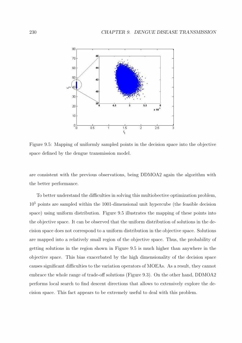
230 CHAPTER 9. DENGUE DISEASE TRANSMISSION
Figure 9.5: Mapping of uniformly sampled points in the decision space into the objective
space defined by the dengue transmission model.
are consistent with the previous observations, being DDMOA2 again the algorithm with
the better performance.
To better understand the difficulties in solving this multiobective optimization problem,
105 points are sampled within the 1001-dimensional unit hypercube (the feasible decision
space) using uniform distribution. Figure 9.5 illustrates the mapping of these points into
the objective space. It can be observed that the uniform distribution of solutions in the de-
cision space does not correspond to a uniform distribution in the objective space. Solutions
are mapped into a relatively small region of the objective space. Thus, the probability of
getting solutions in the region shown in Figure 9.5 is much higher than anywhere in the
objective space. This bias exacerbated by the high dimensionality of the decision space
causes significant difficulties to the variation operators of MOEAs. As a result, they cannot
embrace the whole range of trade-off solutions (Figure 9.3). On the other hand, DDMOA2
performs local search to find descent directions that allows to extensively explore the de-
cision space. This fact appears to be extremely useful to deal with this problem.

9.3. MULTIOBJECTIVE APPROACH 231
0 0.5 1 1.5 2 2.5 30
2
4
6
8
infected humans
cont
rol
40
50
60nondominated solutionsCase ACase BCase CCase D
Figure 9.6: Trade-off curve for the infected population and the control.
For this particular problem, the above analysis allows to conclude that DDMOA2 works
significantly better than the other tested algorithms. However, from a decision maker’s
perspective, instead of comparing the performance of the EMO algorithms, the main con-
cern is a set of optimal solutions. Therefore, all obtained nondominated solutions produced
by the algorithms are combined and a set of nondominated solutions is selected from the
composed multiset. Figure 9.6 presents all nondominated solutions obtained afterwards.
Observing this figure, one can see that for the insecticide cost in the range 0 ≤ f2 ≤ 4
there is almost linear dependency between the total infected human population (f1) and
the insecticide cost (f2). Hence, reducing the number of infected humans from the worst
scenario to 0.5 can be done at a relatively low cost. However, starting from some further
point, say f1 = 0.5, reducing the number of infected humans can be achieved through ex-
ponential increase in spendings for insecticide. Thus, even a small decrease in the number
of infected humans corresponds to a high increase in expenses for insecticide. Scenarios
represented by this part of the trade-off curve can be unacceptable from the economical
point of view.

232 CHAPTER 9. DENGUE DISEASE TRANSMISSION
0 10 20 30 40 50 60 70 80 900
0.5
1
1.5
2
2.5
3
3.5
4x 10
−3
t
I h
(a) Case A
0 10 20 30 40 50 60 70 80 900
0.5
1
1.5
2
2.5
3
3.5
4x 10
−3
t
I h
(b) Case B
0 10 20 30 40 50 60 70 80 900
0.01
0.02
0.03
0.04
0.05
0.06
0.07
0.08
0.09
0.1
t
I h
(c) Case C
0 10 20 30 40 50 60 70 80 900
0.01
0.02
0.03
0.04
0.05
0.06
0.07
0.08
0.09
0.1
t
I h
(d) Case D
Figure 9.7: Different scenarios of the dengue epidemic.
Furthermore, Figure 9.6 depicts four distinct points (Case A, Case B, Case C,
Case D) representing different parts of the trade-off curve, and, consequently, different
scenarios of the dengue epidemic. For each case, Figure 9.7 plots the dynamics of the
numbers of infected humans over the considered period of time.
Thus, Case A represents the medical perspective, when the number of infected humans
is the lowest. From Figure 9.7(a), one can see that the number of infected people decreases
from the very beginning. However, it is achieved through a huge expense for the insecticide.
Case B represents a point in the trade-off curve where an exponential dependency
between the infected humans and the total control begins. From Figure 9.7(b), it can be
9.4. SUMMARY 233
seen that at the beginning the number of infected humans decreases slightly. Thereafter,
it grows steadily.
Case C represents a point located close to the part of the trade-off curve with seemingly
linear dependency between the two objectives. Figure 9.7(b) shows that in this case the
number of infected humans grows from the very first moment. A more rapid grow is
observed in the second half of the considered period of time.
Finally, Case D represents the economical perspective, when the treatment for infected
population is neglected and the main concern is the saving from not performing insecticide
campaigns. Figure 9.7(d) illustrates that in Case D the number of infected humans grows
rapidly from the very beginning, reaching its peak approximately on the 60-th day. After
that the number of infected people decreases. This case corresponds to the worst scenario
from the medical point of view.
9.4 Summary
This chapter presents a multiobjective approach to find an optimal control for reducing
financial expenses caused by the outbreak of the dengue epidemic. The problem includes
two clearly conflicting objectives. The first objective represents expenses due to the infected
population. The second objective represents the total cost of applying insecticide in order
to fight the disease.
Additionally, the performance comparison of DDMOA2 with other state-of-the-art
EMO algorithms is carried out on this problem. The obtained results show that DDMOA2
significantly outperforms the other considered algorithms. DDMOA2 is able to present a
wide range of trade-off solutions, whereas the other tested EMO algorithms face significant
difficulties in solving this problem: the obtained solutions are located in small regions of
the objective space, thus, presenting only a limited amount of alternatives.
The obtained nondominated solutions reveal different perspectives on applying insecti-
cide: a low number of infected humans can be achieved spending larger financial recourses,
whereas low spendings for prevention campaigns result in significant portions of the pop-

234 CHAPTER 9. DENGUE DISEASE TRANSMISSION
ulation affected by the disease. At the same time, a number of other solutions represent
different trade-offs between the given objectives. Once the whole range of optimal solutions
is obtained, the final decision on the control strategy can be made taking into considera-
tion the available financial resources and goals of public health care. Hence, multiobjective
optimization presents clear advantages over other approaches to find an optimal control
strategy.

Chapter 10
Wastewater Treatment Plant Design
The high costs associated with the design and operation of wastewater treatment plants
(WWTPs) motivate the research in the area of WWTP modelling and the water treatment
process optimization. This chapter addresses different methodologies, which are based
on defining and simultaneously optimizing several conflicting objectives, for finding the
optimal values of the state variables in the WWTP design.
10.1 Activated Sludge System
A typical WWTP is schematically represented in Figure 10.1. There is a primary treatment,
which is a physical process and aims to eliminate the gross solids and grease, so avoiding
the blocking up of the secondary treatment. Although the dimensioning of such a unit is
usually empirical and based on the wastewater to be treated, its cost is not affected by
the (biological, chemical and biochemical) characteristics of the wastewater. The cost just
corresponds to the civil engineering construction work of a tank. This is the reason why
this process usually is not included in the optimization procedure. The next two units
define the secondary treatment of the wastewater. This is the most important treatment
in the plant because it eliminates the soluble pollutants. In the majority of the WWTPs,
it is a biological process which, in the case herein studied, comprises an aeration tank and
235

236 CHAPTER 10. WASTEWATER TREATMENT PLANT DESIGN
Figure 10.1: Schematic representation of a typical WWTP (adapted from [23]).
a clarifier that aims to separate the biological sludge from the treated water. There are
other biological and chemical treatments but this is, by far, the most widely used. Finally,
the last unit is used to treat the biological sludge that is wasted by the secondary settler.
When the wastewater is very polluted and the secondary treatment does not provide the
demanded quality, a tertiary treatment, usually a chemical process, can be included. There
are many other possible WWTP layouts, but most of them are alike the above described.
The work herein presented focus solely on the secondary treatment, in particular on
an activated sludge system that is represented in Figure 10.2. This system consists of an
aeration tank and a secondary settler. The influent enters the aeration tank where the
biological reactions take place, in order to remove the dissolved carbonaceous matter and
nitrogen. The sludge that leaves this tank enters the secondary settler where suspended
solids are removed. After this treatment, the treated final effluent leaves the settling tank
and half of the thickened sludge is recycled back to the aeration tank and the rest of it is
Figure 10.2: Schematic representation of the activated sludge system (adapted from the
GPS-X simulator [23]).

10.2. MATHEMATICAL MODEL 237
wasted. The mathematical models used to describe the aeration tank and the settling tank
are the ASM1 model [83], and the ATV model [63] combined with the double exponential
model [172], respectively.
10.2 Mathematical Model
The mathematical model can be subdivided into seven types of equations. The system
under study consists of an aeration tank, where the biological reactions take place, and a
secondary settler for the sedimentation of the sludge and clarification of the effluent.
To describe the aeration tank, the activated sludge model n.1 (ASM1) described by
Henze et al. [83] is used. ASM1 considers both the elimination of the carbonaceous matter
and the removal of the nitrogen compounds. This model is widely accepted by the scientific
community, as it produces good predictive values by simulation [2]. This means that all
state variables keep their biological interpretation. The tank is considered a completely
stirred tank reactor (CSTR) in steady state.
For the settling tank, a combination of the ATV design procedure [63] with the dou-
ble exponential model model [172] is used. The ATV model is usually used as a design
procedure to new WWTPs. It is based on empirical equations obtained by experiments
and does not contain any solid balances, although it contemplates peak wet weather flow
(PWWF) events. The double exponential model model is the most widely used in simula-
tions and it produces results very close to reality. However, since it does not provide extra
sedimentation area needed during PWWF events, the resulting design has to consider the
use of security factors that yield an over-dimensioned and expensive unit.
In [151], it is shown that this combined model is prepared to overcome PWWF events
without over dimensioning and provides the most equilibrated WWTP design when com-
pared with the other two used separately. When these three designs were introduced in
the GPS-X simulator [23] and a stress condition of a PWWF value of five times the normal
flow was imposed, only the combined model was able to support this adverse condition
maintaining the quality of the effluent under the values imposed by the portuguese law.

238 CHAPTER 10. WASTEWATER TREATMENT PLANT DESIGN
Mass Balances around Aeration Tank
The first set of equations come from the mass balances around the aeration tank. The
Peterson matrix of the ASM1 model [83] is used to define the model for the mass balances.
For a CSTR, it is assumed that the mass of a given component entering the tank minus
the mass of the same compound in the tank, plus a reaction term (positive or negative)
equals the accumulation in the tank of the same compound:
Q
Va(ξin − ξ) + rξ =
dξ
dt. (10.2.1)
It is convenient to refer that in a CSTR the concentration of a compound is the same
at any point inside the reactor and at the effluent of that reactor. The reaction term for
the compound in question, rξ, is obtained by the sum of the product of the stoichiometric
coefficients, νξj, with the expression of the process reaction rate, ρj, of the ASM1 Peterson
matrix [83]
rξ =∑j
νξjρj. (10.2.2)
In steady state, the accumulation term given by dξdt
is zero, because the concentration of
a given compound is constant in time. The ASM1 model involves 8 processes incorporating
13 different components. The mass balances for the inert materials, SI and XI , are not
considered because they are transport-only components.
All the symbols used in the WWTP modelling are listed in the Appendix. The process
rates are the following:
• Aerobic growth of heterotrophs
ρ1 = µH
(SS
KS + SS
)(SO
KOH + SO
)XBH ; (10.2.3)
• Anoxic growth of heterotrophs
ρ2 = µH
(SS
KS + SS
)(KOH
KOH + SO
)(SNO
KNO + SNO
)ηgXBH ; (10.2.4)

10.2. MATHEMATICAL MODEL 239
• Aerobic growth of autotrophs
ρ3 = µA
(SNH
KNH + SNH
)(SO
KOA + SO
)XBA; (10.2.5)
• Decay of heterotrophs
ρ4 = bHXBH ; (10.2.6)
• Decay of autotrophs
ρ5 = bAXBA; (10.2.7)
• Ammonification of soluble organic nitrogen
ρ6 = kaSNDXBH ; (10.2.8)
• Hydrolysis of entrapped organics
ρ7 = kh
XSXBH
KX+XSXBH
[(SO
KOH+SO
)+ηh
(KOH
KOH+SO
)(SNO
KNO+SNO
)]XBH ;
(10.2.9)
• Hydrolysis of entrapped organic nitrogen
ρ8 = ρ7XND
XS
. (10.2.10)
The unit adopted for concentration is g COD/m3 and the equations obtained from the
ASM1 model with mass balances are as follows:
• Soluble substrate (SS)
Q
Va(SSin − SS)− 1
YHρ1 −
1
YHρ2 + ρ7 = 0; (10.2.11)
• Slowly biodegradable substrate (XS)
Q
Va(XSin −XS) + (1− fP )ρ4 + (1− fP )ρ5 − ρ7 = 0; (10.2.12)
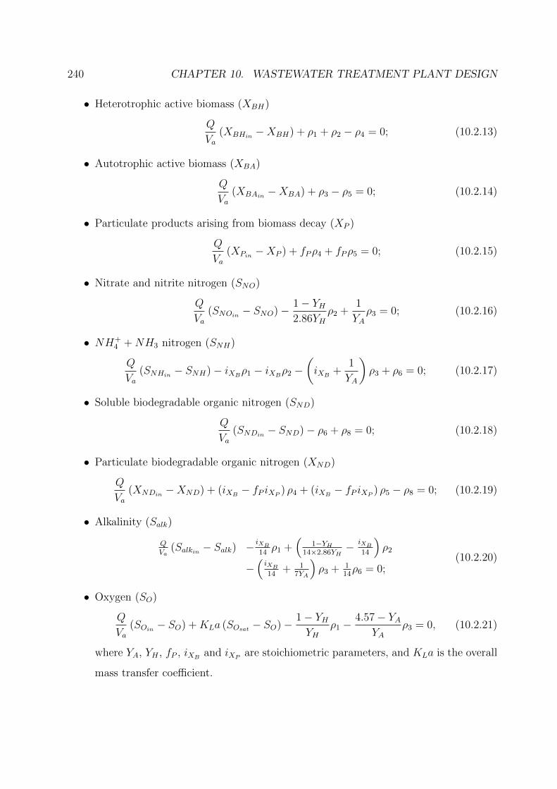
240 CHAPTER 10. WASTEWATER TREATMENT PLANT DESIGN
• Heterotrophic active biomass (XBH)
Q
Va(XBHin −XBH) + ρ1 + ρ2 − ρ4 = 0; (10.2.13)
• Autotrophic active biomass (XBA)
Q
Va(XBAin −XBA) + ρ3 − ρ5 = 0; (10.2.14)
• Particulate products arising from biomass decay (XP )
Q
Va(XPin −XP ) + fPρ4 + fPρ5 = 0; (10.2.15)
• Nitrate and nitrite nitrogen (SNO)
Q
Va(SNOin − SNO)− 1− YH
2.86YHρ2 +
1
YAρ3 = 0; (10.2.16)
• NH+4 +NH3 nitrogen (SNH)
Q
Va(SNHin − SNH)− iXBρ1 − iXBρ2 −
(iXB +
1
YA
)ρ3 + ρ6 = 0; (10.2.17)
• Soluble biodegradable organic nitrogen (SND)
Q
Va(SNDin − SND)− ρ6 + ρ8 = 0; (10.2.18)
• Particulate biodegradable organic nitrogen (XND)
Q
Va(XNDin −XND) + (iXB − fP iXP ) ρ4 + (iXB − fP iXP ) ρ5 − ρ8 = 0; (10.2.19)
• Alkalinity (Salk)
QVa
(Salkin − Salk) −iXB14ρ1 +
(1−YH
14×2.86YH− iXB
14
)ρ2
−(iXB14
+ 17YA
)ρ3 + 1
14ρ6 = 0;
(10.2.20)
• Oxygen (SO)
Q
Va(SOin − SO) +KLa (SOsat − SO)− 1− YH
YHρ1 −
4.57− YAYA
ρ3 = 0, (10.2.21)
where YA, YH , fP , iXB and iXP are stoichiometric parameters, and KLa is the overall
mass transfer coefficient.

10.2. MATHEMATICAL MODEL 241
For oxygen mass transfer, aeration by diffusion is considered:
KLa =α GS η PO2 1333.3
VaSOsatθ(T−20) (10.2.22)
where
SOsat =1777.8β ρPO2
HenryO2
, (10.2.23)
ρ = 999.96(2.29× 10⁻²T )− (5.44× 10⁻³T 2), (10.2.24)
HenryO2 = 708 T + 25700, (10.2.25)
GS is the air flow rate and α, β, ρ, η, PO2 , T and θ are operational parameters [22].
Composite Variables
In a real system, some state variables are, most of the time, not available from direct
measurements. Thus, readily measured composite variables are used instead. They are
defined as follows:
• Particulate chemical oxygen demand
X = XI +XS +XBH +XBA +XP ; (10.2.26)
• Soluble chemical oxygen demand
S = SI + SS; (10.2.27)
• Chemical oxygen demand
COD = X + S; (10.2.28)
• Volatile suspended solids
V SS =X
icv; (10.2.29)

242 CHAPTER 10. WASTEWATER TREATMENT PLANT DESIGN
• Total suspended solids
TSS = V SS + ISS; (10.2.30)
• Biochemical oxygen demand
BOD = fBOD (SS +XS +XBH +XBA) ; (10.2.31)
• Total nitrogen of Kjeldahl
TKN = SNH + SND +XND + iXB (XBH +XBA) + iXP (XP +XI) ; (10.2.32)
• Total nitrogen
N = TKN + SNO; (10.2.33)
where icv and fBOD define ratios to convert units.
Quality Constraints
Quality constraints are usually derived from environmental law restrictions. The most used
are related with limits in COD, N , and TSS at the effluent. In mathematical terms, these
constraints are defined as:
CODef ≤ CODlaw
Nef ≤ Nlaw (10.2.34)
TSSef ≤ TSSlaw
where the subscript “ef” stands for effluent.
Secondary Settler Constraints
Traditionally, the importance of the secondary settler is underestimated when compared
with the aeration tank. However, it plays a crucial role in the activated sludge system. For
example, the clarification efficiency of the settling tank has great influence on the treatment
plant efficiency because the particulate fraction arising from biomass contributes to the

10.2. MATHEMATICAL MODEL 243
major portion of the effluent COD. Further, it has been observed that the investment
cost of a typical settling tank in a WWTP context could reach 25% of the total [73].
Thus, when trying to reduce both investment and operation costs, the importance of the
secondary settler is by far emphasized.
When the wastewater leaves the aeration tank, where the biological treatment took
place, the treated water should be separated from the biological sludge, otherwise, the
COD would be higher than it is at the entry of the system. The most common way of
achieving this purpose is by sedimentation in tanks.
A good settling tank has to accomplish three different functions. As a thickener, it
aims to produce a continuous underflow of thickened sludge to return to the aeration tank;
as a clarifier, it produces a good quality final effluent; and as a storage tank it allows the
conservation of the sludge in peak flow events. None of these functions could fail. If that
happens the effluent will be of poor quality and the overall behavior of the system can be
compromised.
The behavior of a settling tank depends on its design and operation, namely the hy-
draulic features, as the flow rate, the physical features, as inlet and sludge collection
arrangements, site conditions, as temperature and wind, and sludge characteristics. The
factors that most influence the size of the tank are the wastewater flow and the character-
istics of the sludge. As the influent flow is known, the optimization of the sedimentation
area and depth must rely on the sludge characteristics, which in turn are related with the
performance of the aeration tank. So, the operation of the biological reactor influences
directly the performance of the settling tank and for that reason, one should never be
considered without the other.
The ATV design procedure contemplates the PWWF events, in which the sludge mass
transferred from the biological reactor is ∆X Va, where ∆X is the change in the sludge
concentration within the aeration tank. A reduction of 30% on the sludge concentration
for a PWWF event is considered. A higher reduction of the sludge concentration into the
biological reactor may compromise the entire process.

244 CHAPTER 10. WASTEWATER TREATMENT PLANT DESIGN
Figure 10.3: Typical solids concentration-depth profile adopted by the ATV design
procedure (adapted from [63]).
A way of turning around this problem is to allocate a certain depth (h3 from Figure 10.3)
to support the fluctuation of solids during these events. Thus, the sludge storage depth
depends on the mass that needs to be stored during a PWWF and is given by
h3 = ∆XVaDSV I
480As, (10.2.35)
where As is the sedimentation area and DV SI is the diluted sludge volume index. When
this zone is considered, a reduction in the sedimentation area is allowed.
The transferred sludge causes the biological sludge concentration in the reactor at
PWWF to decline, which allows a higher overflow rate and therefore a smaller surface
area. However, the greater the decrease in reactor concentration is, the greater is the
mass of sludge to be stored in the settler tank, so the deeper the tank needs to be. The
ATV procedure allows a trade-off between surface area and depth and one may select the
area/depth combination that suites better the particular site under consideration.
The compaction zone, h4, where the sludge is thickened in order to achieve the conve-
nient concentration to return to the biological reactor, depends only on the characteristics

10.2. MATHEMATICAL MODEL 245
of the sludge, and is given by
h4 = XpDSV I
1000(10.2.36)
where Xp is the sludge concentration in the biological reactor during a PWWF event.
The clear water zone, h1, and the separation zone, h2, are set empirically to 1 m
(h1 + h2 = 1). The depth of the settling tank, h, is the sum of these four zones.
The sedimentation area is still related to the peak flow, Qp, by the expression
Qp
As≤ 2400 (XpDSV I)−1.34 . (10.2.37)
The double exponential model assumes a one dimensional settler, in which the tank is
divided into ten layers of equal thickness (Figure 10.4). Some simplifications are considered.
No biological reactions take place in this tank, meaning that the dissolved matter concen-
tration is maintained across all the layers. Only vertical flux is considered and the solids
are uniformly distributed across the entire cross-sectional area of the feed layer (j = 7).
This model is based on a traditional solids flux analysis but the flux in a particular layer
is limited by what can be handled by the adjacent layer. The settling function, described
by Takacs et al. in [172], which represents the settling velocity, is given by
νs,j = max (0,min (ν ′0, w0)) (10.2.38)
where νs,j is the settling velocity in layer j,
w0 = ν0
(e−rh(TSSj−fnsTSSa) − e−rp(TSSj−fnsTSSa)
), (10.2.39)
TSSj is the total suspended solids concentration in each of the ten considered layers of the
settler, TSSa is the TSS in the feed layer (TSSa = TSS7) and ν0, ν ′0, rh, rp and fns are
the settling parameters [23].
The solids flux due to the bulk movement of liquid may be up or down, νup and νdn

246 CHAPTER 10. WASTEWATER TREATMENT PLANT DESIGN
Figure 10.4: Solids balance around the settler layers according to the double exponential
model (adapted from [172]).
respectively, depending on its position relative to the feed layer, thus
νup =Qef
Asand νdn =
Qr +Qw
As. (10.2.40)
The subscript “r” is concerned with the recycled sludge and “w” refers to the wasted
sludge.
The sedimentation flux, Js, for the layers under the feed layer (j = 7, . . . , 10) is given

10.2. MATHEMATICAL MODEL 247
by
Js,j = νs,jTSSj (10.2.41)
and above the feed layer (j = 1, . . . , 6) the clarification flux, Jclar, is given by
Jclar,j =
νs,jTSSj if TSSj+1 ≤ TSSt
min(νs,jTSSj, νs,j+1TSSj+1) otherwise(10.2.42)
where TSSt is the threshold concentration of the sludge. The resulting solids balances
around each layer, considering steady state, are the following:
• for the layers above the feed layer (j = 1, . . . , 6)
νup(TSSj+1 − TSSj) + Jclar,j−1 − Jclar,jh/10
= 0, (10.2.43)
• for the feed layer (j = 7)
Q TSSaAs
+ Jclar,j−1 − (νup + νdn)TSSj −min(Js,j, Js,j+1)
h/10= 0, (10.2.44)
• for the intermediate layers under the feed layer (j = 8, . . . , 10)
νdn(TSSj−1 − TSSj) + min(Js,j, Js,j−1)−min(Js,j, Js,j+1)
h/10= 0. (10.2.45)
By convention, Jclar,0 = Js,11 = 0.
The use of the combination of these two models to describe the secondary settler is
prepared to turn around the PWWF events without over dimensioning and overcomes the
limitations and powers the advantages of each one.
Flow and Mass Balances
The system behavior, in terms of concentration and flows, may be predicted by balances.
In order to achieve a consistent system, these balances must be done around the entire
system and not only around each unit operation. This is crucial to reinforce the robust-
ness of the model. Furthermore, these balances may not be a sum of the mass balances

248 CHAPTER 10. WASTEWATER TREATMENT PLANT DESIGN
of the individual components since the PWWF events are contemplated in the ATV de-
sign included in the settler modelling. The balances were done to the suspended matter,
dissolved matter and flows.
In the case of the suspended matter, the mass balances concern the organic (X) and
inorganic (XII) solids:
(1 + r)QinfXin = QinfXinf + (1 + r)QinfX −VaX
SRT Xr
(Xr −Xef )−QinfXef , (10.2.46)
Qinf0.2TSSinf =VaXII
SRT Xr
(XIIr −XIIef
)+QinfXIIef , (10.2.47)
where r is the recycle rate. The subscripts “inf” and “in” denote the influent and the
entry of the aeration tank, respectively.
The balances of the dissolved matter are done for each one of the dissolved components
SS, SO, SNO, SNH , SND, Salk, as shown below in the SS case:
(1 + r)QinfSSin = QinfSSinf + rQinfSSr . (10.2.48)
Besides the mass balances, flow balances are also necessary:
Q = Qinf +Qr and Q = Qef +Qr +Qw. (10.2.49)
System Variables Definition
To complete the model, some definitions are added:
• Sludge retention time
SRT =VaX
QwXr
; (10.2.50)
• Hydraulic retention time
HRT =VaQ
; (10.2.51)
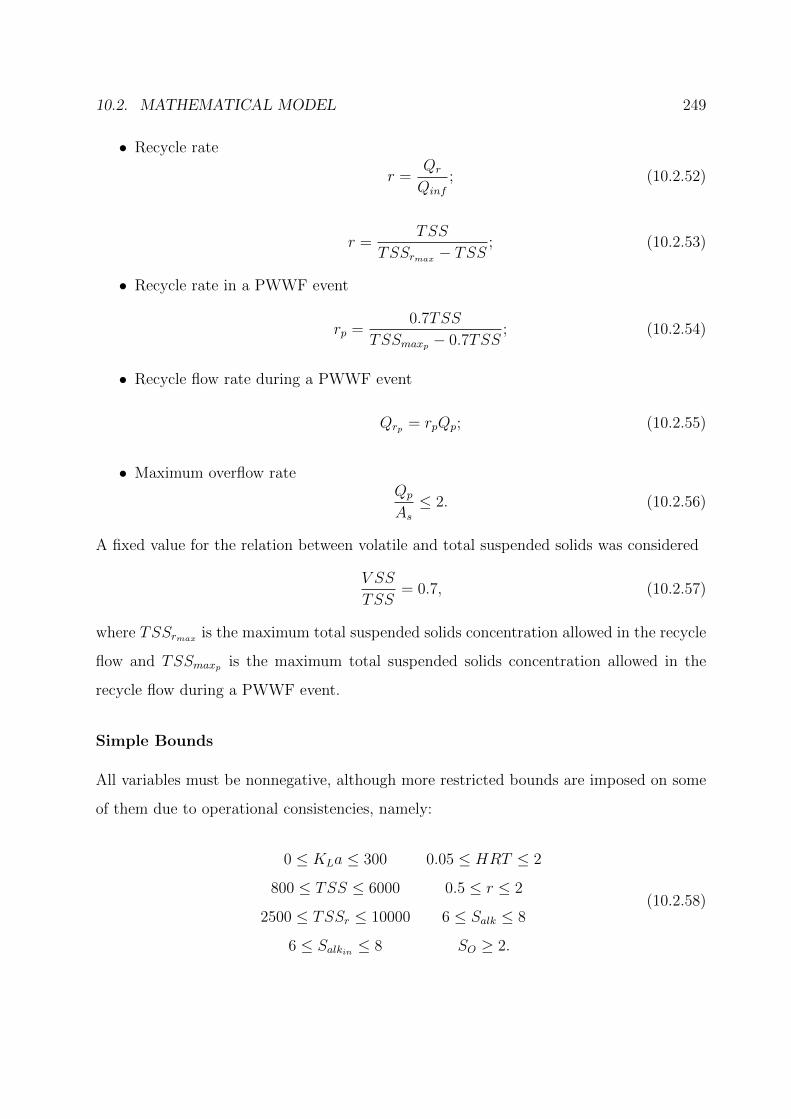
10.2. MATHEMATICAL MODEL 249
• Recycle rate
r =Qr
Qinf
; (10.2.52)
r =TSS
TSSrmax − TSS; (10.2.53)
• Recycle rate in a PWWF event
rp =0.7TSS
TSSmaxp − 0.7TSS; (10.2.54)
• Recycle flow rate during a PWWF event
Qrp = rpQp; (10.2.55)
• Maximum overflow rateQp
As≤ 2. (10.2.56)
A fixed value for the relation between volatile and total suspended solids was considered
V SS
TSS= 0.7, (10.2.57)
where TSSrmax is the maximum total suspended solids concentration allowed in the recycle
flow and TSSmaxp is the maximum total suspended solids concentration allowed in the
recycle flow during a PWWF event.
Simple Bounds
All variables must be nonnegative, although more restricted bounds are imposed on some
of them due to operational consistencies, namely:
0 ≤ KLa ≤ 300 0.05 ≤ HRT ≤ 2
800 ≤ TSS ≤ 6000 0.5 ≤ r ≤ 2
2500 ≤ TSSr ≤ 10000 6 ≤ Salk ≤ 8
6 ≤ Salkin ≤ 8 SO ≥ 2.
(10.2.58)

250 CHAPTER 10. WASTEWATER TREATMENT PLANT DESIGN
10.3 Multiobjective Approach
In the following, the WWTP design is optimized in terms of a secondary treatment, in
a way that the strict laws on effluent quality are accomplished. In essence, the WWTP
design optimization consists in minimizing the total cost, hereupon denoted by TC, which
is the sum of investment and operation costs, and maximizing the effluent quality measured
by a quality index function, represented by the variable QI.
Total Cost Function
The cost function represents the total cost and includes both investment and operation
costs. For the sake of simplicity, no pumps are considered, which means that all the flows
in the system move by the effect of gravity. The total cost is given by the sum of the
investment (IC) and operation (OC) costs. To obtain a cost function based on portuguese
real data, a study was carried out with a WWTP building company. The basic structure
of the model is C = aZb [176], where a and b are parameters that depend on the region
where the WWTP is being built, and have to be estimated. Variable Z is the characteristic
of the unit operation that is influencing the cost, for example, the volume Va and the air
flow GS for the case of the aeration tank. Parameters a and b were estimated by a least
squares technique, giving the following investment cost function for the aeration tank:
ICa = 148.6V 1.07a + 7737G0.62
S . (10.3.1)
The operation cost is usually estimated on an annual basis, so it has to be updated to
a present value using the updating term Γ:
Γ =N∑j=1
1
(1 + i)j=
1− (1 + i)−N
i, (10.3.2)
where i represents the discount rate (rate of return), i.e., the rate that is used to valuing
a project using the concept of the time value of money, over a certain amount of time,
for example, N years. This is also taken as the average life-expectancy of a WWTP. In
this study, i = 0.05 and N = 20 years are used. Since the collected data come from a

10.3. MULTIOBJECTIVE APPROACH 251
set of WWTPs in design, operation data are not available. However, from the company
experience, the expected life span for the civil engineering construction works is 20 years
and the maintenance expenses are around 1% of the investment costs during the first 10
years and around 2% during the remaining ones. Although the replacement costs of the
electromechanical components are negligible, they are usually replaced after 10 years. The
predominant cost comes from the energy used for pumping the air flow into the aeration
tank. The power cost (Pc) in Portugal is 0.08 e/kWh. With this information and with
the updating term Γ in (10.3.2), the operation cost of the aeration tank is then
OCa =[0.01Γ + 0.02Γ (1 + i)−10] 148.6V 1.07
a +(1 + i)−107737G0.62S +115.1ΓPcGS. (10.3.3)
The term (1 + i)−10 is used to bring to present a future value, in this case, 10 years from
now.
Similarly, the least squares technique is used to fit the basic model to the available
data, and the correspondent investment cost function
ICs = 955.5A0.97s , (10.3.4)
and the operation cost function, that is concerned only with the maintenance for the civil
construction,
OCs =[0.01Γ + 0.02Γ (1 + i)−10] 148.6(As h)1.07 (10.3.5)
are obtained for the settling tank. The objective cost function (TC) is then given by the
sum of all the previous functions:
TC = 174.2V 1.07a + 12487G0.62
S + 114.8GS + 955.5A0.97s + 41.3 (As h)1.07 . (10.3.6)
Quality Index Function
To be able to attain effluent quality at a required level, a quality index function may be
used to measure the amount of pollution in the effluent.
The quality index (QI) defined by the BSM1 model [2] gives a measure of the amount
of daily pollution, in average terms during seven days. It depends on the quality of the

252 CHAPTER 10. WASTEWATER TREATMENT PLANT DESIGN
effluent in terms of the total suspended solids (TSS), the chemical oxygen demand (COD),
the biochemical oxygen demand (BOD), the total Kjeldahl nitrogen (TKN), the nitrate
and nitrite nitrogen (SNO) and the effluent flow (Qef ). The obtained function is:
QI = (2TSS + COD + 2BOD + 20TKN + 2SNO)Qef
1000. (10.3.7)
Experimental Setup
The presented model is coded in the MATLAB R© programming language. The problem
consists of 2 objective functions, 115 decision variables, 1 inequality constraint, and 99
equality constraints. All the variables are bounded below and above. To solve this problem
EMyO-C is used.
In order to handle constraints, the original nondominated sorting used in EMyO-C
is modified introducing the constrained-domination principle [46]. Under this principle,
solution a is said to constrained-dominate solution b, if any of the following conditions is
true: (i) solution a is feasible and solution b is not, (ii) solutions a and b are both infeasible,
but solution a has a smaller overall constraint violation, (iii) solutions a and b are feasible
and solution a dominates solution b. For a given solution, the overall constraint violation
cv is calculated as: cv =p∑i=1
max0 , gi(x)+q∑j=1
|hj(x)|.
The major difficulty in solving this real-world problem is related to the presence of
a larger number of equality constraints. So to successfully solve this highly constrained
problem, the experiments are conducted in several steps. First, 30 independent runs of
EMyO-C were performed with a population size of µ = 1000, running for 1000 generations.
Further parameter settings were the same as discussed in Chapter 8. In each run, the initial
population was randomly generated within the bounds. As a result, no feasible solution
was found. Therefore, all the produced outcomes were combined and one nondominated
solution was selected from the resulting set based on the concept of constrained-domination.
Afterwards, this solution was improved using a single-objective optimizer to find a feasible
solution. For this purpose, HGPSAL was used. After obtaining the feasible solution,
further experiments are conducted using EMyO-C. In this instance, 30 independent runs
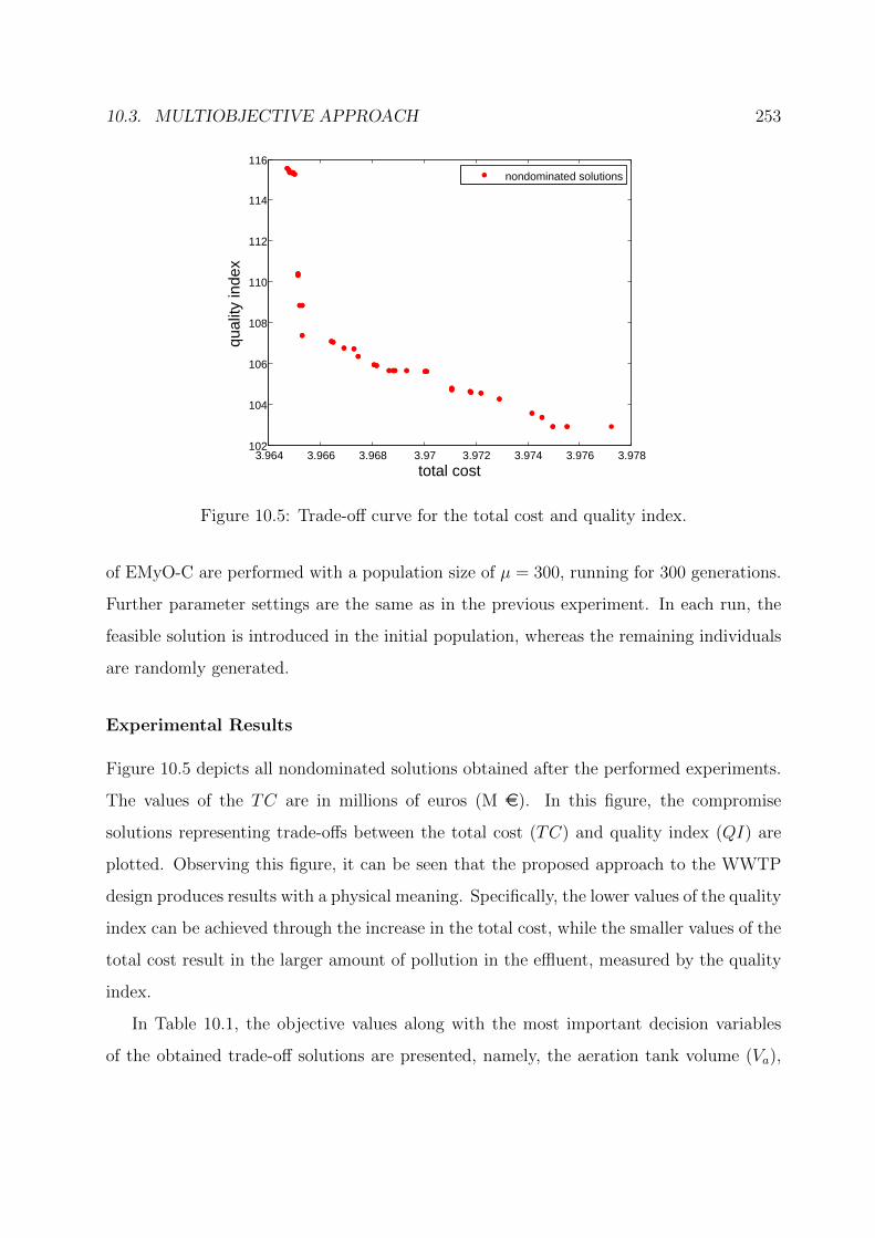
10.3. MULTIOBJECTIVE APPROACH 253
3.964 3.966 3.968 3.97 3.972 3.974 3.976 3.978102
104
106
108
110
112
114
116
total cost
qual
ity in
dex
nondominated solutions
Figure 10.5: Trade-off curve for the total cost and quality index.
of EMyO-C are performed with a population size of µ = 300, running for 300 generations.
Further parameter settings are the same as in the previous experiment. In each run, the
feasible solution is introduced in the initial population, whereas the remaining individuals
are randomly generated.
Experimental Results
Figure 10.5 depicts all nondominated solutions obtained after the performed experiments.
The values of the TC are in millions of euros (M e). In this figure, the compromise
solutions representing trade-offs between the total cost (TC) and quality index (QI) are
plotted. Observing this figure, it can be seen that the proposed approach to the WWTP
design produces results with a physical meaning. Specifically, the lower values of the quality
index can be achieved through the increase in the total cost, while the smaller values of the
total cost result in the larger amount of pollution in the effluent, measured by the quality
index.
In Table 10.1, the objective values along with the most important decision variables
of the obtained trade-off solutions are presented, namely, the aeration tank volume (Va),
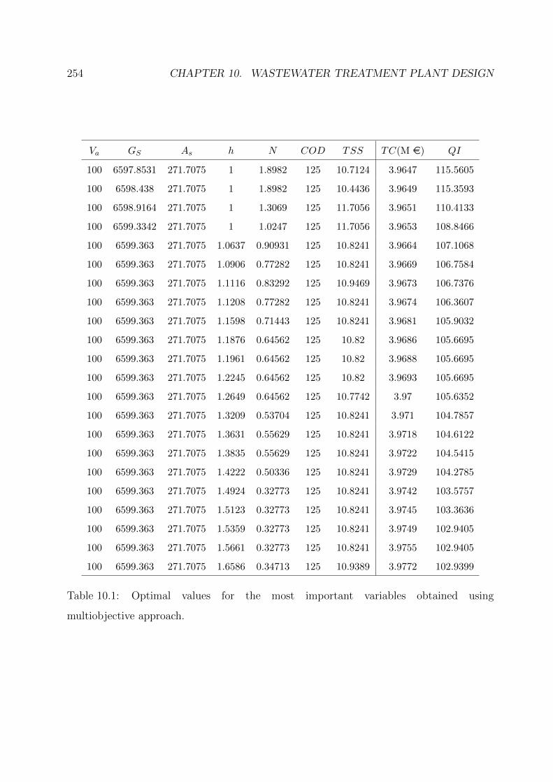
254 CHAPTER 10. WASTEWATER TREATMENT PLANT DESIGN
Va GS As h N COD TSS TC(M e) QI
100 6597.8531 271.7075 1 1.8982 125 10.7124 3.9647 115.5605
100 6598.438 271.7075 1 1.8982 125 10.4436 3.9649 115.3593
100 6598.9164 271.7075 1 1.3069 125 11.7056 3.9651 110.4133
100 6599.3342 271.7075 1 1.0247 125 11.7056 3.9653 108.8466
100 6599.363 271.7075 1.0637 0.90931 125 10.8241 3.9664 107.1068
100 6599.363 271.7075 1.0906 0.77282 125 10.8241 3.9669 106.7584
100 6599.363 271.7075 1.1116 0.83292 125 10.9469 3.9673 106.7376
100 6599.363 271.7075 1.1208 0.77282 125 10.8241 3.9674 106.3607
100 6599.363 271.7075 1.1598 0.71443 125 10.8241 3.9681 105.9032
100 6599.363 271.7075 1.1876 0.64562 125 10.82 3.9686 105.6695
100 6599.363 271.7075 1.1961 0.64562 125 10.82 3.9688 105.6695
100 6599.363 271.7075 1.2245 0.64562 125 10.82 3.9693 105.6695
100 6599.363 271.7075 1.2649 0.64562 125 10.7742 3.97 105.6352
100 6599.363 271.7075 1.3209 0.53704 125 10.8241 3.971 104.7857
100 6599.363 271.7075 1.3631 0.55629 125 10.8241 3.9718 104.6122
100 6599.363 271.7075 1.3835 0.55629 125 10.8241 3.9722 104.5415
100 6599.363 271.7075 1.4222 0.50336 125 10.8241 3.9729 104.2785
100 6599.363 271.7075 1.4924 0.32773 125 10.8241 3.9742 103.5757
100 6599.363 271.7075 1.5123 0.32773 125 10.8241 3.9745 103.3636
100 6599.363 271.7075 1.5359 0.32773 125 10.8241 3.9749 102.9405
100 6599.363 271.7075 1.5661 0.32773 125 10.8241 3.9755 102.9405
100 6599.363 271.7075 1.6586 0.34713 125 10.9389 3.9772 102.9399
Table 10.1: Optimal values for the most important variables obtained using
multiobjective approach.

10.4. MANY-OBJECTIVE APPROACH 255
the air flow rate (GS), the sedimentation area (As), the settler tank depth (h), the total
nitrogen (N), the chemical oxygen demand (COD), the total suspended solid (TSS). The
presented solutions are obtained after applying clustering procedure to group the data in
the objective space. This way, each solution represents a distinct cluster, hence a different
part of the trade-off curve. This procedure allows to reduce the number of points, thereby
facilitating the visualization of the results. Thus, different design perspectives can be easily
observed from the obtained solutions.
It can be seen that the aeration tank volume and the sedimentation area maintain the
same values in all the presented solutions. Only the slight variation in a few solutions is
observed concerning the air flow rate, whereas the settler depth has the larger variation in
the values between all the variables composing the cost function. This hints that the lower
cost as well as the desirable values of the quality index can be mostly achieved through
controlling the settler depth. Furthermore, it can be seen that the chemical oxygen demand
is at the highest allowable level (125), whereas the total nitrogen and the total suspended
solid are far below the law limits (15 and 35, respectively).
10.4 Many-Objective Approach
In the following, the WWTP design is optimized by simultaneously minimizing the vari-
ables that influence the operation and investment costs as well as the quality index func-
tion. These variables are referred as to the influential variables. This approach results in
a many-objective optimization problem.
Influential Variables
To avoid the use of cost functions that are time and local dependent, four objective func-
tions, each describing a variable that influences the investment and operation costs of a
WWTP, in each unit operation, are used.
As far as the aeration tank is concerned, the variables that mostly influence the costs
are the volume (Va) and the air flow (GS). In terms of investment, the first variable

256 CHAPTER 10. WASTEWATER TREATMENT PLANT DESIGN
influences directly the cost of the construction of the tank, and the second influences the
required power of the air pumps. In terms of operation, both variables will determine
the power needed to aerate the sludge properly, as well as the maintenance, in terms of
electromechanical and civil construction material, due to deterioration.
As to the secondary settler, and assuming that the settling process is only due to the
gravity, the variables that most influence the costs are the sedimentation area (As) and
the tank depth (h), for obvious reasons.
Concerning the quality index function, each variable on the right-hand side of (10.3.7) is
considered as a distinct function, thereby adding to the optimization problem six different
objectives.
Experimental Setup
The problem is coded in the MATLAB R© programming language. This time, the problem
consists of 10 objective functions, 115 decision variables, 1 inequality constraint, and 99
equality constraints. All the variables are bounded below and above. To solve this prob-
lem, 30 independent runs of EMyO-C are performed with a population size of µ = 300,
running for 750 generations. Further parameter settings are the same as in the previous ex-
periment. In each run, the feasible solution is introduced in the initial population, whereas
the remaining individuals are randomly generated.
Experimental Results
The clustering procedure is used to group all nondominated solutions in the objective
space. Table 10.2 presents the most important variables and the objective function values
for a representative of each cluster. Additionally, the values of the total cost (TC) and
the quality index (QI) are calculated for these solutions. From the table, it can seen that
the values of the aeration tank volume, the sedimentation area as well as the nitrate and
nitrite nitrogen are constant for all the presented solutions. The values of the chemical
oxygen demand are slightly reduced compared with that obtained using the multiobjective

10.4. MANY-OBJECTIVE APPROACH 257Va
GS
As
hN
COD
TSS
BOD
TKN
SNO
Qef
TC
(Me
)QI
100
6594
.302
327
1.70
751
2.81
61
124.2
268
11.8
656
61.1
615
2.8
064
0.0
802
374.6
088
3.9
633
122.8
764
100
6594
.302
327
1.70
751
2.81
71
124.1
447
19.2
583
61.0
899
2.8
064
0.0
802
374.6
306
3.9
633
128.3
383
100
6594
.302
327
1.70
751
2.84
53
124.3
486
29.1
979
57.9
506
2.8
064
0.0
802
373.5
855
3.9
633
133.1
374
100
6594
.302
327
1.70
751
2.95
06
124.2
268
11.3
468
61.2
184
2.8
064
0.0
802
373.7
916
3.9
633
122.2
631
100
6599
.363
271.
7075
13.
2074
123.4
647
34.0
113
60.1
686
3.2
387
0.0
802
373.2
369
3.9
653
141.1
593
100
6589
.241
627
1.70
751.
3647
2.19
74125
19.7
987
60.7
109
1.9
417
0.0
802
373.4
868
3.9
678
121.9
279
100
6594
.302
327
1.70
751.
3849
3.20
28123.3
74
25.6
511
61.0
103
3.2
387
0.0
802
374.5
473
3.9
702
135.9
887
100
6599
.363
271.
7075
1.30
362.
4526
124.1
36
15.4
315
60.4
597
2.3
74
0.0
802
373.1
675
3.9
707
121.2
809
100
6599
.363
271.
7075
1.43
513.
2256
122.8
556
34.5
301
61.0
103
3.2
387
0.0
802
374.0
567
3.9
731
142.2
592
100
6594
.302
327
1.70
751.
5554
2.95
8123.6
176
15.4
219
61.1
504
2.8
064
0.0
802
373.6
879
3.9
733
124.9
963
100
6599
.363
271.
7075
1.50
612.
106
124.5
326
34.5
059
60.7
304
1.9
417
0.0
802
373.3
003
3.9
744
132.6
874
100
6594
.302
327
1.70
751.
6622
2.14
92124.5
326
12.1
456
59.9
099
2.3
74
0.0
802
374.1
559
3.9
753
118.8
802
100
6599
.363
271.
7075
1.55
542.
958
122.8
556
30.1
749
61.1
504
2.8
064
0.0
802
374.2
245
3.9
753
135.9
325
100
6599
.363
271.
7075
1.55
582.
4022
125
16.2
075
60.6
728
2.3
74
0.0
802
373.0
643
3.9
753
122.3
076
100
6594
.302
327
1.70
751.
6879
3.05
18123.6
599
19.0
348
60.8
003
2.8
064
0.0
802
377.0
701
3.9
757
128.6
042
100
6599
.363
271.
7075
1.62
982.
8089
122.9
04
32.9
028
61.0
551
2.8
064
0.0
802
373.8
48
3.9
767
137.7
822
100
6599
.363
271.
7075
1.62
982.
958
123.3
74
31.3
109
60.5
197
2.8
064
0.0
802
373.3
762
3.9
767
136.1
953
100
6599
.363
271.
7075
1.68
792.
9973
123.9
122
19.0
348
60.8
003
2.8
064
0.0
802
373.2
73.9
777
127.4
023
100
6589
.241
627
1.70
751.
9295
3.27
03124.6
942
19.2
583
61.6
308
2.8
064
0.0
802
373.3
365
3.9
782
128.5
04
100
6594
.302
327
1.70
751.
927
2.86
89124.3
001
13.7
515
60.7
982
3.2
387
0.0
802
373.5
766
3.9
802
126.9
33
Tab
le10
.2:
Opti
mal
valu
esfo
rth
em
ost
imp
orta
nt
vari
able
sob
tain
edusi
ng
man
y-o
bje
ctiv
eap
pro
ach.
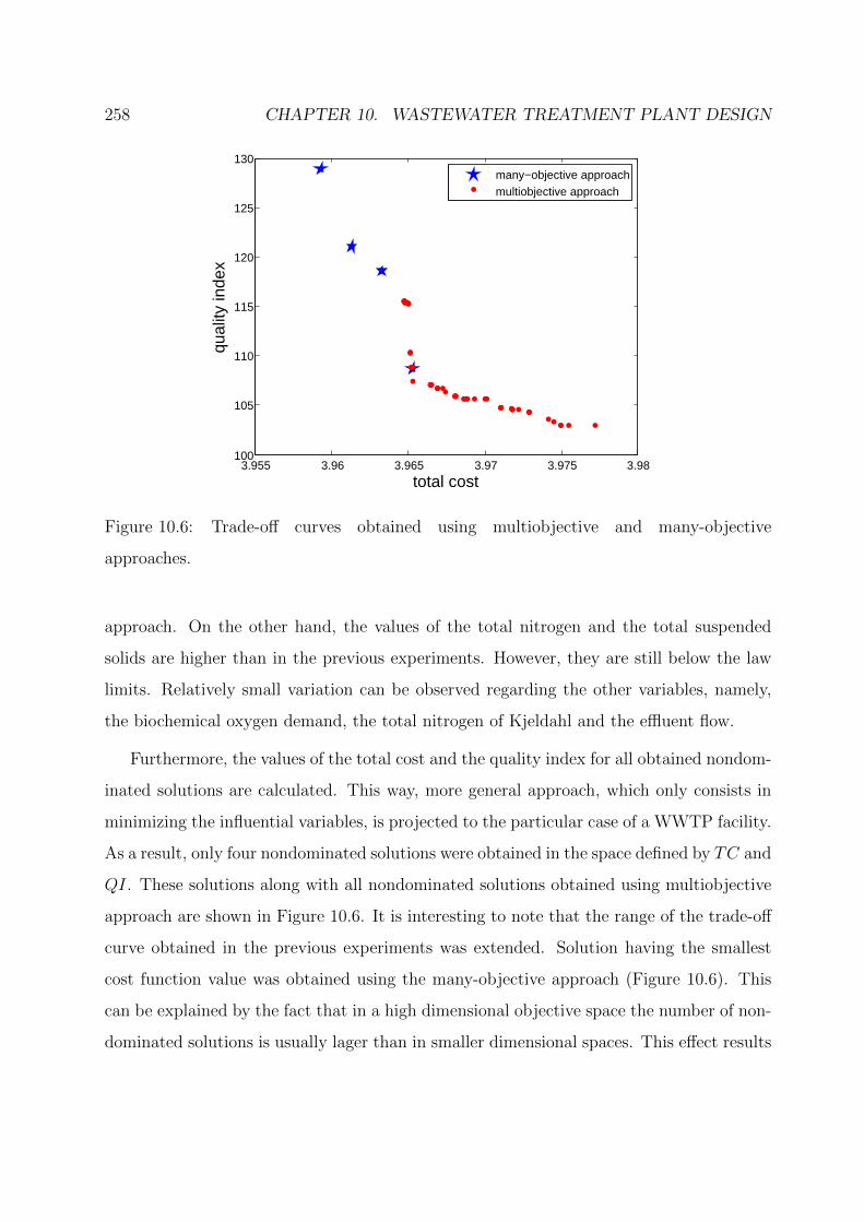
258 CHAPTER 10. WASTEWATER TREATMENT PLANT DESIGN
3.955 3.96 3.965 3.97 3.975 3.98100
105
110
115
120
125
130
total cost
qual
ity in
dex
many−objective approachmultiobjective approach
Figure 10.6: Trade-off curves obtained using multiobjective and many-objective
approaches.
approach. On the other hand, the values of the total nitrogen and the total suspended
solids are higher than in the previous experiments. However, they are still below the law
limits. Relatively small variation can be observed regarding the other variables, namely,
the biochemical oxygen demand, the total nitrogen of Kjeldahl and the effluent flow.
Furthermore, the values of the total cost and the quality index for all obtained nondom-
inated solutions are calculated. This way, more general approach, which only consists in
minimizing the influential variables, is projected to the particular case of a WWTP facility.
As a result, only four nondominated solutions were obtained in the space defined by TC and
QI. These solutions along with all nondominated solutions obtained using multiobjective
approach are shown in Figure 10.6. It is interesting to note that the range of the trade-off
curve obtained in the previous experiments was extended. Solution having the smallest
cost function value was obtained using the many-objective approach (Figure 10.6). This
can be explained by the fact that in a high dimensional objective space the number of non-
dominated solutions is usually lager than in smaller dimensional spaces. This effect results

10.5. SUMMARY 259
in the propagation of the dissimilarities between solutions in the decision space. Typically,
this is an undesirable feature that adversely affects the performance of EMO algorithms.
However, the advantageous side effect is that different regions of the search space can be
explored, which happens to be the case in the herein described experiments. Thus, the
obtained results show that the many-objective approach can be useful not only during a
draft project when the exact data about design of a particular WWTP is not available, but
also for finding optimal values in the later stages of the decision-making process. Defining
and simultaneously optimizing different combinations of objectives can enrich the final set
of the obtained alternatives, which are eventually presented to the decision maker.
10.5 Summary
This chapter addresses new methodologies to model and solve a WWTP design optimiza-
tion problem that can be extended to any WWTP unit operation modelling, regardless
adjusting to each particularity of the problem under study. Two different approaches are
considered. In the first approach, the WWTP design is addressed through a biobjective
optimization problem that consists in minimizing the total cost and the quality index func-
tions. To estimate some model parameters, the real portuguese data were used. Since the
least squares technique needs to be used for parameter estimation, the formulated problem
is time and local dependent. The second approach is more suitable for a draft project,
when the exact location and time where the WWTP is going to be built is still unknown.
The approach consists in simultaneously minimizing influential variables, which results in
a ten-objective optimization problem. After solving this problem, the decision-maker has
a set of alternatives from which he(she) can choose from. This information might help to
elaborate a first version of the project, allowing to study all the alternatives, even with
different unit operations. When the specific location and moment in time are defined, the
analysis based on the minimization of the two objective functions – the total cost and the
quality index – is to be preferred.
The results obtained in this study clearly show that the multiobjective modelling is

260 CHAPTER 10. WASTEWATER TREATMENT PLANT DESIGN
an effective tool to the WWTP design optimization. The achieved optimal solutions are
meaningful in physical terms. Investment and operation costs are highly influenced by
the optimized variables, meaning that the obtained solutions are economically attractive.
Both approaches to WWTP design optimization provide a set of nondominated solutions
from which the decision-maker can choose according to his(her) preferences.

Chapter 11
Conclusions
11.1 Conclusions
Optimization problems involving multiple conflicting objectives are common in the real
world. These problems, called multiobjective optimization problems, contain multiple
conflicting objectives, giving rise to a set of optimal solutions instead of a single optimal
solution. This set is generally known as the Pareto optimal set. The existence of two search
spaces and multiple optimal solutions constitutes the fundamental difference between a
single-objective and multiobjective optimization, making in general the latter more difficult
than the former. Recently, due to their population-based nature evolutionary algorithms
have become a powerful and increasingly popular technique to approximate the Pareto set.
The present thesis investigates the application of EMO algorithms to solve multiob-
jective optimization problems from different perspectives. As new approaches based on
combinations of existing techniques have proved to be successful in single-objective opti-
mization, the bulk of the thesis is dedicated to develop hybrid multiobjective evolutionary
algorithms. Such methods are devised to exploit better features of their single components,
increasing the diversity of the existing approaches, thereby representing a significant con-
tribution in the optimization research area. Since the decision maker is prone to put every
performance index of the underlying problem as a separate objective, optimization prob-
261
262 CHAPTER 11. CONCLUSIONS
lems with a large number of objectives arise continuously in diverse fields of science and
engineering, leading to an increasing demand for efficient approaches capable to handle
such problems. Therefore, a significant effort is spent enforcing the field of many-objective
optimization. As a consequence, two highly competitive selection methods for evolutionary
many-objective optimization are proposed. Since the demand for solving real-world prob-
lems is the main motivation to develop new optimization techniques, the herein developed
algorithms are applied to solve two real-world optimization problems arising from epidemi-
ological and environmental mathematical models, thereby making the contributions of the
thesis relevant in terms of practical applications.
The review of the existing approaches to multiobjective optimization is presented in
Chapter 3. Although different approaches are discussed, the review clearly indicates the
popularity of EMO algorithms. Nevertheless, since their emergence in the mid 1980s and
a wide variety of proposed algorithmic frameworks, almost all existing EMO algorithms
are created by extending single-objective EAs. This is often made by modifying selection
operators of EAs, meanwhile maintaining the same variation operators. There is a rela-
tively limited number of hybrid MOEAs, especially, based on combinations of traditional
evolutionary algorithms and local search methods.
The first attempt to develop a hybrid algorithm for MO is presented in Chapter 5.
The resulting HGPSAL approach uses genetic operators for global search and a pattern
search method to improve solutions, within an augmented Lagrangian framework for con-
strained single-objective optimization. Despite the promising results obtained on SOPs,
the extension of this approach to MO adopting frameworks of the NBI and NC methods
possesses several disadvantages when compared with EMO due to a relatively large number
of function evaluations required for the optimization process.
Further, exploring the direction of hybrid algorithms for MO, two local search-based
approaches are proposed in subsequent chapters. Adopting the idea of Timmel’s classical
method for generating new candidate solutions, DDMOA is introduced in Chapter 6. The
potential strengths of this approach are revealed in comparative studies with some state-
of-the-art EMO algorithms. The proposed procedure to explore the search space appears
11.1. CONCLUSIONS 263
to be highly competitive with different established MOEAs. Employing descent directions
found for each objective to generate offspring makes the reproduction operator of DDMOA
intrinsically multiobjective. It is devised taking into consideration the fundamental nature
of MOPs, i.e., the presence of multiple objectives. On the contrary, most of the exist-
ing EMO algorithms just employ variation operators initially designed for single-objective
optimization.
Motivated by promising results and some identified potential weaknesses of DDMOA,
further research has been conducted in the direction paved by this approach. This results
in the successor of DDMOA, termed DDMOA2, which generalizes the original algorithm,
and is presented in Chapter 7. Although DDMOA2 mainly inherits the way offspring are
generated from its predecessor, significant improvements of the performance are achieved.
Moreover, due to the use of scalarizing fitness assignment DDMOA2 is applicable to solve
problems with more than three-objectives. Although DDMOA2 represents a viable alter-
native for solving MOPs, exhibiting a highly competitive and often superior performance
with respect to the existing approaches, the deterioration of performance is observed when
the number of objectives increases.
Chapter 8 is particularly devoted to many-objective optimization. Adopting the frame-
work of DE, slight modifications are introduced to improve its convergence properties on
multimodal problems. The resulting differential evolution with variable-wise mutation re-
striction is used as the basis for creating efficient many-objective optimization algorithms.
Two different mechanisms to provide necessary selection pressure in a high-dimensional ob-
jective space are developed. The indicator-based approach uses a set of evenly distributed
points on the hyperplane to approximate the Pareto front to calculate distance metrics
based on IGD for solutions in the last accepted non-domination level. This approach ex-
hibits a good performance being capable to converge to the Pareto set for all the tested
problems. The second selection scheme is created as an attempt to obtain a more flexible
and self-adaptive approach for many-objective optimization. Although it shows ability to
guide the population toward the Pareto front in a high-dimensional objective space, the
results on some problems reveal that more computational effort may be eventually required

264 CHAPTER 11. CONCLUSIONS
to obtain more precise approximations. However, results obtained on DTLZ2 and DTLZ7
clearly highlight the advantages of the suggested clustering-based selection scheme. Since
this approach does not require any additional parameters and is polynomial in the number
of objectives, it points a promising direction for future research. Similarly to optimization
algorithms in general, where it is not possible to obtain one solver that performs the best on
all problems, it seems to be difficult, if not impossible, to have the best fitness assignment
and selection scheme to guide the population in the objective space.
The third part of the thesis is concerned with solving real-world problems using EMO
algorithms. The first problem arises from a mathematical model of the dengue disease
transmission, where one seeks to identify the most effective way of applying insecticide
minimizing two conflicting objectives: the total cost due to infected humans and the total
cost of applying insecticide. Additionally, the performance comparison of different EMO
algorithms on this problem is carried out. The obtained results reveal that all of the
used state-of-the-art MOEAs perform poorly, failing to provide a wide range of trade-off
solutions within the given budget. On the other hand, DDMOA2 takes advantage of its
embedded local search procedure that helps to extensively search the high-dimensional
decision space. Even the visual comparison of the trade-off solutions obtained by different
algorithms clearly shows the superiority of DDMOA2 when solving this problem.
Another considered problem arises from optimizing a wastewater treatment plant de-
sign. To solve this problem, different methodologies for finding optimal values of the de-
cision variables are addressed. Although one can define two essential goals in the WWTP
design, namely, reducing the total cost and maximizing the WWTP performance, the
ways for achieving these goals can be different. Thus, a multiobjective approach, based
on a biobjective problem, appears to be an effective way for finding optimal values in the
WWTP design. The obtained set of trade-off solutions gives much more possible alterna-
tives than single-objective approach does. The wide range of trade-off solutions provides
valuable information about the problem, being highly beneficial to the decision-making
process. Aside from the two-objective approach, which is time and local dependent, a
more general approach is considered. Thus, each influential variable is minimized sepa-

11.2. FUTURE PERSPECTIVES 265
rately. Although this approach is mainly conceived for a draft project, the obtained results
reveal that defining and simultaneously optimizing different objectives can be beneficial at
any stage of the decision-making process. In turn, this opens new research opportunities
in the WWTP design area.
The performance analysis of different algorithms on real-world problems is particularly
important. It can reveal strengths and weaknesses of different methodologies, which in
the design phase are often tested only on artificial test functions. Such problems are un-
doubtedly useful, however, they do not possess all the difficulties encountered in real-world
optimization problems. Therefore, careful analysis of algorithms’ performance and inherent
difficulties of real problems constitute a significant contribution to the research. In turn,
the promising results obtained by DDMOA2 on the dengue disease transmission model
highlight the relevance of hybrid approaches to multiobjective optimization. Actually,
they motivate further research in this direction.
11.2 Future Perspectives
Despite the significant advances achieved in the design of EMO algorithms during the last
two decades, and a growing attention to the field of EMO that resulted in a large number of
publications, there are a lot of open issues and opportunities for future research. Thus, the
popular algorithmic frameworks need to be investigated thoroughly to further define their
strengths and weaknesses. Such studies on real-world problems are of particular interest.
As a result, some new frameworks or combinations of the existing frameworks may arise
in the near future. In turn, these new proposals will also rise other new research questions
and opportunities.
Since there are two search spaces in which EAs operate when solving multiobjective op-
timization problems, new advanced operators for performing the search in each space must
be designed. They are essential to successfully deal with increasingly complex real-world
problems. Although the current research in EMO very often focuses on either the man-
aging of the external archive or developing an appropriate selection strategy to guide the

266 CHAPTER 11. CONCLUSIONS
search, new fitness assignment and selection procedures capable to maintain the diversity
among the population members and to assure the convergence to the Pareto set in difficult
problem environments must be investigated. This is especially relevant to problems with
a large number of objectives.
Moreover, there is a continuous demand for efficient variation operators, which are cru-
cial to the performance of either single-objective or multiobjective optimization algorithms.
A substantial amount of work must still be done to successfully handle multimodal, ill-
conditioned, nonseparable, deceptive problems. Although there exists a variety of EAs with
different offspring generation strategies that are successful in single-objective optimization,
their extensions to the multiobjective case may correspond to a poor performance. How-
ever, the current research in evolutionary computation community is mainly based on using
the same variation operators in single-objective and multiobjective optimization. Further-
more, hybridization of evolutionary algorithms with local search methods in multiobjective
optimization is another promising research direction, which until now seems to receive rel-
atively small attention.
Another important issue that highly affects the performance of EMO algorithms is how
to properly choose several control parameters for the algorithms. Usually, the parameters
are predefined based on algorithmic or problem knowledge. They also can be determined as
a result of an empirical study, where a set of suitable parameters is chosen after performing
repeated tests with different settings. However, in real-world applications, especially with
computationally expensive function evaluations, this strategy may not be applicable. Thus,
new strategies to adaptively tune control parameters need to be investigated. This idea
can also be applied to search strategies either in the decision or objective space, where the
best suitable among available strategies is chosen in different phases of the search process.

Bibliography
[1] H. A. Abbass, R. Sarker, and C. Newton. A Pareto-frontier differential evolution
approach for multi-objective optimization problems. In Proceedings of the IEEE
Congress on Evolutionary Computation, CEC’01, pages 971–978, 2001.
[2] J. Alex, L. Benedetti, J. Copp, K. V. Gernaey, U. Jeppsson, I. Nopens, M. N. Pons,
C. Rosen, J. P. Steyer, and P. Vanrolleghem. Benchmark simulation model no. 1
(BSM1). Technical report, IWA Taskgroup on Benchmarking of Control Strategies
for WWTPs, 2008.
[3] Md. Asafuddoula, T. Ray, and R. Sarker. A decomposition based evolutionary al-
gorithm for many objective optimization with systematic sampling and adaptive
epsilon control. In Proceedings of the Conference on Evolutionary Multi-Criterion
Optimization, EMO’13, pages 413–427, 2013.
[4] T. Back, U. Hammel, and H. P. Schwefel. Evolutionary computation: Comments
on the history and current state. IEEE Transactions on Evolutionary Computation,
1(1):3–17, 1997.
[5] J. Bader. Hypervolume-based search for multiobjective optimization: Theory and
methods. PhD thesis, Swiss Federal Institute of Technology, Zurich, Switzerland,
2010.
267

268 BIBLIOGRAPHY
[6] J. Bader, K. Deb, and E. Zitzler. Faster hypervolume-based search using Monte Carlo
sampling. In Proceedings of the Conference on Multiple Criteria Decision Making,
MCDM’08, pages 313–326, 2008.
[7] J. Bader and E. Zitzler. HypE: An algorithm for fast hypervolume-based many-
objective optimization. Evolutionary Computation, 19(1):45–76, 2011.
[8] S. Bandyopadhyay, U. Maulik, and M. K. Pakhira. Clustering using simulated anneal-
ing with probabilistic redistribution. Journal of Pattern Recognition and Artificial
Intelligence, 15(2):269–285, 2001.
[9] S. Bandyopadhyay, S. Saha, U. Maulik, and K. Deb. A simulated annealing-based
multiobjective optimization algorithm: AMOSA. IEEE Transactions on Evolution-
ary Computation, 12(3):269–283, 2008.
[10] A. Banks, J. Vincent, and C. Anyakoha. A review of particle swarm optimization.
Part I: background and development. Natural Computing, 6(4):467–484, 2007.
[11] A. Banks, J. Vincent, and C. Anyakoha. A review of particle swarm optimization.
Part II: hybridisation, combinatorial, multicriteria and constrained optimization, and
indicative applications. Natural Computing, 7(1):109–124, 2008.
[12] D. P. Bertsekas. Nonlinear Programming. Athena Scientific, Belmont, 2 edition,
1999.
[13] N. Beume, B. Naujoks, and M. Emmerich. SMS-EMOA: Multiobjective selec-
tion based on dominated hypervolume. European Journal of Operational Research,
181(3):1653–1669, 2007.
[14] H.-G. Beyer. The theory of evolution strategies. Springer-Verlag, New York, USA,
2001.
[15] H.-G. Beyer and H.-P. Schwefel. Evolution strategies: A comprehensive introduction.
Natural Computing, 1(1):3–52, 2002.

BIBLIOGRAPHY 269
[16] S. Bleuler, M. Laumanns, L. Thiele, and E. Zitzler. PISA: A platform and program-
ming language independent interface for search algorithms. In Proceedings of the
Conference on Evolutionary Multi-Criterion Optimization, EMO’03, pages 494–508,
2003.
[17] P. A. N. Bosman and D. Thierens. The balance between proximity and diversity in
multiobjective evolutionary algorithms. IEEE Transactions on Evolutionary Com-
putation, 7(2):174–188, 2003.
[18] K. Bringmann, T. Friedrich, F. Neumann, and M. Wagner. Approximation-guided
evolutionary multi-objective optimization. In Proceedings of the International Joint
Conference on Artificial Intelligence, pages 1198–1203, 2011.
[19] D. Brockhoff and E. Zitzler. Are all objectives necessary? On dimensionality reduc-
tion in evolutionary multiobjective optimization. In Proceedings of the Conference
on Parallel Problem Solving from Nature, PPSN’06, pages 533–542, 2006.
[20] D. Brockhoff and E. Zitzler. Improving hypervolume-based multiobjective evolution-
ary algorithms by using objective reduction methods. In Proceedings of the IEEE
Congress on Evolutionary Computation, CEC’07, pages 2086–2093, 2007.
[21] D. Brockhoff and E. Zitzler. Objective reduction in evolutionary multiobjective opti-
mization: Theory and applications. Evolutionary Computation, 17(2):135–166, 2009.
[22] Hydromantis Inc. Canada. GPS-X user’s guide, 2001.
[23] Hydromantis Inc. Canada. Gps-x v4.1. http://www.hydromantis.com/software02.html,
2002.
[24] E. G. Carrano, E. F. Wanner, and R. H. C. Takahashi. A multicriteria statistical
based comparison methodology for evaluating evolutionary algorithms. IEEE Trans-
actions on Evolutionary Computation, 15(6):848–870, 2011.
270 BIBLIOGRAPHY
[25] P. Cattand, P. Desjeux, M. G. Guzman, J. Jannin, A. Kroeger, A. Medici, P. Mus-
grove, M. B. Nathan, A. Shaw, and C. J. Schofield. Tropical Diseases Lacking Ade-
quate Control Measures: Dengue, Leishmaniasis, and African Trypanosomiasis. Con-
trol Priorities in Developing Countries. DCPP, 2 edition, 2006.
[26] R. Caves, S. Quegan, and R. White. Quantitative comparison of the performance of
SAR segmentation algorithms. Transactions on Image Processing, 7(11):1534–1546,
1998.
[27] C. Chen, Y. Chen, and Q. Zhang. Enhancing MOEA/D with guided mutation and
priority update for multi-objective optimization. In Proceedings of the IEEE Congress
on Evolutionary Computation, CEC’09, pages 209–216, 2009.
[28] T. Chiang and Y. Lai. MOEA/D-AMS: Improving MOEA/D by an adaptive mating
selection mechanism. In Proceedings of the IEEE Congress on Evolutionary Compu-
tation, CEC’11, pages 1473–1480, 2011.
[29] C. A. Coello Coello, G. B. Lamont, and D. A. Van Veldhuizen. Evolutionary Algo-
rithms for Solving Multi-Objective Problems. Genetic and Evolutionary Computation.
Springer, 2 edition, 2007.
[30] C. A. Coello Coello, G. T. Pulido, and M. S. Lechuga. Handling multiple objectives
with particle swarm optimization. IEEE Transactions on Evolutionary Computation,
8(3):256–279, 2004.
[31] A. R. Conn, N. I. M. Gould, and P. L. Toint. A globally convergent augmented
Lagrangian algorithm for optimization with general constraints and simple bounds.
SIAM Journal on Numerical Analysis, 28(2):545–572, 1991.
[32] D. W. Corne and J. D. Knowles. Techniques for highly multiobjective optimisation:
Some nondominated points are better than others. In Proceedings of the Conference
on Genetic and Evolutionary Computation, GECCO’07, pages 773–780, 2007.

BIBLIOGRAPHY 271
[33] L. Costa, I. Espırito Santo, and P. Oliveira. Stochastic algorithms assessment using
performance profiles. In Proceedings of the Conference on Genetic and Evolutionary
Computation, GECCO’11, pages 933–940, 2011.
[34] L. Costa and P. Oliveira. An adaptive sharing elitist evolution strategy for multiob-
jective optimization. Evolutionary Computation, 11(4):417–438, 2003.
[35] L. Costa, I. A. C. P. Espırito Santo, R. Denysiuk, and E. M. G. P. Fernandes.
Hybridization of a genetic algorithm with a pattern search augmented Lagrangian
method. In Proceedings of the Conference on Engineering Optimization, EngOpt’10,
page 1195, 2010.
[36] A. L. Custodio, J. F. A. Madeira, A. I. F. Vaz, and L. N. Vicente. Direct multisearch
for multiobjective optimization. SIAM Journal on Optimization, 21(3):1109–1140,
2011.
[37] P. Czyzak and A. Jaszkiewicz. Pareto simulated annealing - a metaheuristic technique
for multiple-objective combinatorial optimization. Journal of Multi-Criteria Decision
Analysis, 7(1):34–47, 1998.
[38] N. O. Da Cunha and E. Polak. Constrained minimization under vector-valued criteria
in finite dimensional spaces. Journal of Mathematical Analysis and Applications,
9(1):103–124, 1967.
[39] I. Das and J. E. Dennis. Normal-boundary intersection: A new method for generating
the Pareto surface in nonlinear multicriteria optimization problems. SIAM Journal
on Optimization, 8(3):631–657, 1998.
[40] S. Das and P. N. Suganthan. Differential evolution: A survey of the state-of-the-art.
IEEE Transactions on Evolutionary Computation, 15(1):4–31, 2011.
[41] K. Deb. Multi-objective genetic algorithms: Problem difficulties and construction of
test problems. Evolutionary Computation, 7(3):205–230, 1999.
272 BIBLIOGRAPHY
[42] K. Deb. Multi-Objective Optimization using Evolutionary Algorithms. Wiley-
Interscience Series in Systems and Optimization. John Wiley & Sons, 2001.
[43] K. Deb and R. B. Agrawal. Simulated binary crossover for continuous search space.
Complex Systems, 9:115–148, 1995.
[44] K. Deb and H. Jain. Handling many-objective problems using an improved NSGA-
II procedure. In Proceedings of the IEEE Congress on Evolutionary Computation,
CEC’12, pages 1–8, 2012.
[45] K. Deb, K. Miettinen, and S. Chaudhuri. Toward an estimation of nadir objective
vector using a hybrid of evolutionary and local search approaches. IEEE Transactions
on Evolutionary Computation, 14(6):821–841, 2010.
[46] K. Deb, A. Pratap, S. Agarwal, and T. Meyarivan. A fast and elitist multiobjec-
tive genetic algorithm: NSGA-II. IEEE Transactions on Evolutionary Computation,
6(2):182–197, 2002.
[47] K. Deb and D. K. Saxena. Searching for Pareto-optimal solutions through dimension-
ality reduction for certain large-dimensional multi-objective optimization problems.
In Proceedings of the World Congress on Computational Intelligence, WCCI’06, pages
3352–3360, 2006.
[48] K. Deb, A. Sinha, and S. Kukkonen. Multi-objective test problems, linkages, and evo-
lutionary methodologies. Technical Report 2006001, Indian Institute of Technology,
Kanpur, India, 2006.
[49] K. Deb and J. Sundar. Reference point based multi-objective optimization using evo-
lutionary algorithms. In Proceedings of the Conference on Genetic and Evolutionary
Computation, GECCO’06, pages 635–642, 2006.
[50] K. Deb, L. Thiele, M. Laumanns, and E. Zitzler. Scalable test problems for evolu-
tionary multi-objective optimization. Technical Report 112, Swiss Federal Institute
of Technology, Zurich, Switzerland, 2001.
BIBLIOGRAPHY 273
[51] K. Deb, L. Thiele, M. Laumanns, and E. Zitzler. Scalable multi-objective optimiza-
tion test problems. In Proceedings of the IEEE Congress on Evolutionary Computa-
tion, CEC’02, pages 825–830, 2002.
[52] R. Denysiuk, L. Costa, and I. Espırito Santo. DDMOA: Descent directions based
multiobjective algorithm. In Proceedings of the Conference on Computational and
Mathematical Methods in Science and Engineering, CMMSE’12, pages 460–471, 2012.
[53] R. Denysiuk, L. Costa, and I. Espırito Santo. DDMOA2: Improved descent
directions-based multiobjective algorithm. In Proceedings of the Conference on Com-
putational and Mathematical Methods in Science and Engineering, CMMSE’13, pages
513–524, 2013.
[54] R. Denysiuk, L. Costa, and I. Espırito Santo. Many-objective optimization using
differential evolution with variable-wise mutation restriction. In Proceedings of the
Conference on Genetic and Evolutionary Computation, GECCO’13, pages 591–598,
2013.
[55] R. Denysiuk, L. Costa, and I. Espırito Santo. A new hybrid evolutionary multiob-
jective algorithm guided by descent directions. Journal of Mathematical Modelling
and Algorithms in Operations Research, 12(3):233–251, 2013.
[56] M. Derouich, A. Boutayeb, and E. Twizell. A model of dengue fever. Biomedical
Engineering Online, 2(4):1–10, 2003.
[57] J. Derrac, S. Garcıa, D. Molina, and F. Herrera. A practical tutorial on the use
of nonparametric statistical tests as a methodology for comparing evolutionary and
swarm intelligence algorithms. Swarm and Evolutionary Computation, 1(1):3–18,
2011.
[58] G. J. Devine, E. Z. Perea, G. F. Killen, J. D. Stancil, S. J. Clark, and A. C. Morrison.
Using adult mosquitoes to transfer insecticides to aedes aegypti larval habitats. In

274 BIBLIOGRAPHY
Proceeding of the National Academy of Sciences of the United States of America,
2009.
[59] E. D. Dolan and J. J. More. Benchmarking optimization software with performance
profiles. Mathematical Programming, 91(2):201–213, 2002.
[60] N. Drechsler, R. Drechsler, and B. Becker. Multi-objective optimisation based on
relation favour. In Proceedings of the Conference on Evolutionary Multi-Criterion
Optimization, EMO’01, pages 154–166, 2001.
[61] J. J. Durillo, J. Garcıa-Nieto, A. J. Nebro, C. A. Coello Coello, F. Luna, and E. Alba.
Multi-objective particle swarm optimizers: An experimental comparison. In Proceed-
ings of the Conference on Evolutionary Multi-Criterion Optimization, EMO’09, pages
495–509, 2009.
[62] J. J. Durillo and A. J. Nebro. jMetal: A Java framework for multi-objective opti-
mization. Advances in Engineering Software, 42(10):760–771, 2011.
[63] G. A. Ekama, J. L. Barnard, F. W. Gunthert, P. Krebs, J. A. McCrquodale D. S.
Parker, and E. J. Wahlberg. Secondary settling tanks: Theory, modelling, design and
operation. Technical Report 6, IAWQ - International Association on Water Quality,
1997.
[64] M. Emmerich, N. Beume, and N. Boris. An EMO algorithm using the hypervolume
measure as selection criterion. In Proceedings of the Conference on Evolutionary
Multi-Criterion Optimization, EMO’05, pages 62–76, 2005.
[65] M. T. M. Emmerich and A. H. Deutz. Test problems based on Lame superspheres.
In Proceedings of the Conference on Evolutionary Multi-Criterion Optimization,
EMO’07, pages 922–936, 2007.
[66] L. Esteva and H. M. Yang. Mathematical model to assess the control of aedes aegypti
mosquitoes by the sterile insect technique. Mathematical Biosciences, 198:132–147,
2005.
BIBLIOGRAPHY 275
[67] M. Farina, K. Deb, and P. Amato. Dynamic multiobjective optimization problems:
test cases, approximations, and applications. IEEE Transactions on Evolutionary
Computation, 8(5):425–442, 2004.
[68] M. Fleischer. The measure of Pareto optima applications to multi-objective meta-
heuristics. In Proceedings of the Conference on Evolutionary Multi-Criterion Opti-
mization, EMO’03, pages 519–533, 2003.
[69] P. J. Fleming, R. C. Purshouse, and R. J. Lygoe. Many-objective optimization: An
engineering design perspective. In Proceedings of the Conference on Evolutionary
Multi-Criterion Optimization, EMO’05, pages 14–32, 2005.
[70] C. M. Fonseca and P. J. Fleming. Genetic algorithms for multiobjective optimization:
Formulation, discussion and generalization. In Proceedings of the Conference on
Genetic Algorithms, pages 416–423, 1993.
[71] C. M. Fonseca and P. J. Fleming. On the performance assessment and comparison
of stochastic multiobjective optimizers. In Proceedings of the Conference on Parallel
Problem Solving from Nature, PPSN’96, pages 584–593, 1996.
[72] C. M. M. Fonseca. Multiobjective Genetic Algorithms with Application to Control
Engineering Problems. PhD thesis, University of Sheffield, UK, 1995.
[73] X.-S. Qin G.-H. Huang G.-M. Zeng, S.-F. Zhang and J.-B. Li. Application of nu-
merical simulation on optimum design of two-dimensional sedimentation tanks in
the wastewater treatment plant. Journal of Environmental Sciences, 15(3):346–350,
2003.
[74] S. Garcıa, D. Molina, M. Lozano, and F. Herrera. A study on the use of non-
parametric tests for analyzing the evolutionary algorithms’ behaviour: A case study
on the CEC’2005 special session on real parameter optimization. Journal of Heuris-
tics, 15(6):617–644, 2009.

276 BIBLIOGRAPHY
[75] S. Gass and T. Saaty. The computational algorithm for the parametric objective
function. Naval Research Logistics Quarterly, 2(1):39–45, 1955.
[76] F. Glover. Heuristics for integer programming using surrogate constraints. Decision
Sciences, 8:156–166, 1977.
[77] D. E. Goldberg. Genetic Algorithms in Search, Optimization and Machine Learning.
Addison-Wesley, Boston, USA, 1989.
[78] Y. Y. Haimes, L. S. Lasdon, and D. A. Wismer. On a bicriterion formulation of
the problems of integrated system identification and system optimization. IEEE
Transactions on Systems, Man and Cybernetics, 1(3):296–297, 1971.
[79] M. P. Hansen and A. Jaszkiewicz. Evaluating the quality of approximations to
the non-dominated set. Technical Report IMM-REP-1998-7, Technical University of
Denmark, Copenhagen, Denmark, 1998.
[80] N. Hansen and A. Ostermeier. Adapting arbitrary normal mutation distributions in
evolution strategies: The covariance matrix adaptation. In Proceedings of the IEEE
Conference on Evolutionary Computation, CEC’96, pages 312–317, 1996.
[81] N. Hansen and A. Ostermeier. Completely derandomized self-adaptation in evolution
strategies. Evolutionary Computation, 9(2):159–195, 2001.
[82] M. Hapke, A. Jaszkiewicz, and R. Slowinski. Pareto simulated annealing for fuzzy
multi-objective combinatorial optimization. Journal of Heuristics, 6(3):329–345,
2000.
[83] M. Henze, C. P. L. Grady Jr, W. Gujer, G. V. R. Marais, and T. Matsuo. Acti-
vated sludge model no. 1. Technical report, IAWPRC Task Group on Mathematical
Modelling for design and operation of biological wastewater treatment, 1986.
BIBLIOGRAPHY 277
[84] Y. C. Ho and D. L. Pepyne. Simple explanation of the no-free-lunch theorem and
its implications. Journal of Optimization Theory and Applications, 115(3):549–570,
2002.
[85] J. H. Holland. Adaptation in Natural and Artificial Systems. MIT Press, Ann Arbor,
MI, 1975.
[86] R. Hooke and T. A. Jeeves. Direct search solution of numerical and statistical prob-
lems. Journal on Associated Computation, 8(2):212–229, 1961.
[87] S. Huband, P. Hingston, L. Barone, and L. While. A scalable multi-objective test
problem toolkit. In Proceedings of the Conference on Evolutionary Multi-Criterion
Optimization, EMO’05, pages 280–295, 2005.
[88] S. Huband, P. Hingston, L. Barone, and L. While. A review of multiobjective test
problems and a scalable test problem toolkit. IEEE Transactions on Evolutionary
Computation, 10(5):477–506, 2006.
[89] S. Huband, P. Hingston, L. White, and L. Barone. An evolution strategy with
probabilistic mutation for multi-objective optimisation. In Proceedings of the IEEE
Congress on Evolutionary Computation, CEC’03, pages 2284–2291, 2003.
[90] E. J. Hughes. Multiple single objective Pareto sampling. In Proceedings of the IEEE
Congress on Evolutionary Computation, CEC’03, pages 2678–2684, 2003.
[91] E. J. Hughes. Evolutionary many-objective optimisation: Many once or one many?
In Proceedings of the IEEE Congress on Evolutionary Computation, CEC’05, pages
222–227, 2005.
[92] E. J. Hughes. MSOPS-II: A general-purpose many-objective optimiser. In Proceedings
of the IEEE Congress on Evolutionary Computation, CEC’07, pages 3944–3951, 2007.
278 BIBLIOGRAPHY
[93] E. J. Hughes. Many-objective directed evolutionary line search. In Proceedings of the
Conference on Genetic and Evolutionary Computation, GECCO’11, pages 761–768,
2011.
[94] C. Igel, N. Hansen, and S. Roth. Covariance matrix adaptation for multi-objective
optimization. Evolutionary Computation, 15(1):1–28, 2007.
[95] C. Igel, T. Suttorp, and N. Hansen. Steady-state selection and efficient covariance
matrix update in the multi-objective CMA-ES. In Proceedings of the Conference on
Evolutionary Multi-Criterion Optimization, EMO’07, 2007.
[96] A. W. Iorio and X. Li. Solving rotated multi-objective optimization problems using
differential evolution. In Proceedings of the Australian Joint Conference on Artificial
Intelligence, pages 861–872, 2004.
[97] H. Ishibuchi, T. Doi, and Y. Nojima. Incorporation of scalarizing fitness functions
into evolutionary multiobjective optimization algorithms. In Proceedings of the Con-
ference on Parallel Problem Solving from Nature, PPSN’06, pages 493–502, 2006.
[98] H. Ishibuchi and T. Murata. Multi-objective genetic local search algorithm and
its application to flowshop scheduling. IEEE Transactions on Systems, Man and
Cybernetics, 28(3):392–403, 1998.
[99] H. Ishibuchi and Y. Nojima. Optimization of scalarizing functions through evolution-
ary multiobjective optimization. In Proceedings of the Conference on Evolutionary
Multi-Criterion Optimization, EMO’07, pages 51–65, 2007.
[100] H. Ishibuchi, Y. Sakane, N. Tsukamoto, and Y. Nojima. Simultaneous use of different
scalarizing functions in MOEA/D. In Proceedings of the Conference on Genetic and
Evolutionary Computation, GECCO’10, pages 519–526, 2010.
[101] H. Ishibuchi, N. Tsukamoto, and Y. Nojima. Iterative approach to indicator-based
multiobjective optimization. In Proceedings of the IEEE Congress on Evolutionary
Computation, pages 3967–3974, 2007.

BIBLIOGRAPHY 279
[102] H. Ishibuchi, N. Tsukamoto, and Y. Nojima. Evolutionary many-objective opti-
mization: A short review. In Proceedings of the IEEE Congress on Evolutionary
Computation, CEC’08, 2008.
[103] H. Ishibuchi, T. Yoshida, and T. Murata. Balance between genetic search and local
search in memetic algorithms for multiobjective permutation flowshop scheduling.
IEEE Transactions on Evolutionary Computation, 7(2):204–223, 2003.
[104] H. Jain and K. Deb. An improved adaptive approach for elitist nondominated sorting
genetic algorithm for many-objective optimization. In Proceedings of the Conference
on Evolutionary Multi-Criterion Optimization, EMO’13, pages 307–321, 2013.
[105] A. Jaszkiewicz. Genetic local search for multi-objective combinatorial optimization.
European Journal of Operational Research, 137(1):50–71, 2002.
[106] V. J. Bowman Jr. On the relationship of the Chebyshev norm and the efficient
frontier of multiple criteria objectives. Lecture Notes in Economics and Mathematical
Systems, 130:76–86, 1976.
[107] J. Kennedy and R. Eberhart. Particle swarm optimization. In Proceedings of the
Conference on Neural Networks, volume 4, pages 1942–1948, 1995.
[108] V. R. Khare, X. Yao, and K. Deb. Performance scaling of multi-objective evolution-
ary algorithms. In Proceedings of the Conference on Evolutionary Multi-Criterion
Optimization, EMO’03, pages 376–390, 2003.
[109] S. Kirkpatrick, C. D. Gelatt, and M. P. Vecchi. Optimization by simulated annealing.
Science, 220:671–680, 1983.
[110] J. Knowles and D. Corne. Properties of an adaptive archiving algorithm for storing
nondominated vectors. IEEE Transactions on Evolutionary Computation, 7(2):100–
116, 2003.
280 BIBLIOGRAPHY
[111] J. Knowles, L. Thiele, and E. Zitzler. A tutorial on the performance assessment of
stochastic multiobjective optimizers. Technical Report 214, Computer Engineering
and Networks Laboratory, Swiss Federal Institute of Technology, Zurich, Switzerland,
2006.
[112] J. D. Knowles. Local-Search and Hybrid Evolutionary Algorithms for Pareto Opti-
mization. PhD thesis, University of Reading, UK, 2002.
[113] J. D. Knowles and D. W. Corne. Approximating the nondominated front using the
Pareto archived evolution strategy. Evolutionary Computation, 8(2):149–172, 2000.
[114] M. Koppen and K. Yoshida. Substitute distance assignments in NSGA-II for han-
dling many-objective optimization problems. In Proceedings of the Conference on
Evolutionary Multi-Criterion Optimization, EMO’07, pages 727–741, 2007.
[115] S. Kukkonen and J. Lampinen. An extension of generalized differential evolution for
multi-objective optimization with constraints. In Proceedings of the Conference on
Parallel Problem Solving from Nature, PPSN’04, pages 752–761, 2004.
[116] S. Kukkonen and J. Lampinen. GDE3: the third evolution step of generalized differ-
ential evolution. In Proceedings of the IEEE Congress on Evolutionary Computation,
CEC’05, pages 443–450, 2005.
[117] S. Kukkonen and J. Lampinen. Ranking-dominance and many-objective optimiza-
tion. In Proceedings of the IEEE Congress on Evolutionary Computation, CEC’07,
pages 3983–3990, 2007.
[118] M. Laguna and R. Marti. Scatter Search: Methodology and Implementations in C.
Kluwer Academic Publishers, Norwell, MA, USA, 2002.
[119] J. Lampinen. DE’s selection rule for multiobjective optimization. Technical report,
Lappeenranta University of Technology, Lappeenranta, Finland, 2001.

BIBLIOGRAPHY 281
[120] M. Laumanns, L. Thiele, K. Deb, and E. Zitzler. Combining convergence and
diversity in evolutionary multiobjective optimization. Evolutionary Computation,
10(3):263–282, 2002.
[121] R. M. Lewis and V. Torczon. Pattern search algorithms for bound constrained min-
imization. SIAM Journal on Optimization, 9(4):1082–1099, 1999.
[122] R. M. Lewis and V. Torczon. A globally convergent augmented Lagrangian pattern
search algorithm for optimization with general constraints and simple bounds. SIAM
Journal on Optimization, 12(4):1075–1089, 2002.
[123] H. Li and Q. Zhang. Multiobjective optimization problems with complicated Pareto
sets, MOEA/D and NSGA-II. IEEE Transactions on Evolutionary Computation,
13(2):284–302, 2009.
[124] H. Li, Q. Zhang, E. Tsang, and J. A. Ford. Hybrid estimation of distribution al-
gorithm for multiobjective knapsack problem. In Proceedings of the Conference on
Evolutionary Computation in Combinatorial Optimization, EvoCOP’04, pages 145–
154, 2004.
[125] J. J. Liang, T. P. Runarsson, E. Mezura-Montes, M. Clerc, P. N. Suganthan, C. A.
Coello Coello, and K. Deb. Problem definitions and evaluation criteria for the CEC
2006 special session on constrained real-parameter optimization. Technical report,
School of EEE, Nanyang Technological University, Singapore, 2006.
[126] W. L. Loh. On latin hypercube sampling. Annals of Statistics, 33(6):2058–2080,
1996.
[127] A. Lopez Jaimes, C. A. Coello Coello, and D. Chakraborty. Objective reduction
using a feature selection technique. In Proceedings of the Conference on Genetic and
Evolutionary Computation, GECCO’08, pages 673–680, 2008.
282 BIBLIOGRAPHY
[128] I. Loshchilov, M. Schoenauer, and M. Sebag. Not all parents are equal for MO-CMA-
ES. In Proceedings of the Conference on Evolutionary Multi-Criterion Optimization,
EMO’11, pages 31–45, 2011.
[129] W. K. Mashwani and A. Salhi. A decomposition-based hybrid multiobjective evo-
lutionary algorithm with dynamic resource allocation. Applied Soft Computing,
12(9):2765–2780, 2012.
[130] A. Messac and C. Mattson. Normal constraint method with guarantee of even rep-
resentation of complete Pareto frontier. AIAA Journal, 42:2101–2111, 2004.
[131] E. Mezura-Montes, M. Reyes-Sierra, and C. A. Coello Coello. Multi-objective opti-
mization using differential evolution: A survey of the state-of-the-art. Advances in
Differential Evolution, 143:173–196, 2008.
[132] Z. Michalewicz. Genetic Algorithms + Data Structures = Evolution Programs.
Springer-Verlag, Berlin, 1992.
[133] K. Miettinen. Nonlinear multiobjective optimization, volume 12 of International Se-
ries in Operations Research and Management Science. Kluwer Academic Publishers,
1999.
[134] M. Mitchell. Introduction to Genetic Algorithms. MIT Press, Ann Arbor, MI, 1996.
[135] A. J. Nebro, J. J. Durillo, J. Garcıa-Nieto, C. A. Coello Coello, F. Luna, and E. Alba.
SMPSO: A new PSO-based metaheuristic for multi-objective optimization. In Pro-
ceedings of the Symposium on Computational Intelligence in Multicriteria Decision-
Making, MCDM’09, pages 66–73, 2009.
[136] A. J. Nebro, F. Luna, E. Alba, B. Dorronsoro, J. J. Durillo, and A. Beham. AbYSS:
Adapting scatter search to multiobjective optimization. IEEE Transactions on Evo-
lutionary Computation, 12(4), 2008.

BIBLIOGRAPHY 283
[137] F. Neri and V. Tirronen. Recent advances in differential evolution: A survey and
experimental analysis. Artificial Intelligence Review, 33(1-2):61–106, 2010.
[138] T. Okabe, Y. Jin, M. Olhofer, and B. Sendhoff. On test functions for evolutionary
multi-objective optimization. In Proceedings of the Conference on Parallel Problem
Solving From Nature, PPSN’04, pages 792–802, 2004.
[139] M. Otero, N. Schweigmann, and H. G. Solari. A stochastic spatial dynamical model
for aedes aegypti. Bulletin of Mathematical Biology, 70(5):1297–1325, 2008.
[140] M. Pelikan, D. E. Goldberg, and F. G. Lobo. A survey of optimization by building
and using probabilistic models. Computational Optimization and Applications, 21(1),
2002.
[141] K. Price, R. M. Storn, and J. A. Lampinen. Differential Evolution: A Practical
Approach to Global Optimization. Natural Computing Series. Springer, 2005.
[142] R. C. Purshouse and P. J. Fleming. Evolutionary many-objective optimisation: An
exploratory analysis. In Proceedings of the IEEE Congress on Evolutionary Compu-
tation, CEC’03, pages 2066–2073, 2003.
[143] S. Zhao P. N. Suganthan W. Liu S. Tiwari Q. Zhang, A. Zhou. Multiobjective opti-
mization test instances for the CEC 2009 special session and competition. Technical
Report CES-487, University of Essex, UK, 2009.
[144] S. Rana, S. Jasola, and R. Kumar. A review on particle swarm optimization algo-
rithms and their applications to data clustering. Artificial Intelligence Review, 35(3),
2011.
[145] M. Reyes Sierra and C. A. Coello Coello. Improving pso-based multi-objective op-
timization using crowding, mutation and epsilon-dominance. In Proceedings of the
Conference on Evolutionary Multi-Criterion Optimization, EMO’05, pages 505–519,
2005.
284 BIBLIOGRAPHY
[146] M. Reyes Sierra and C. A. Coello Coello. Multi-objective particle swarm optimizers:
A survey of the state-of-the-art. International Journal of Computational Intelligence
Research, 2(3):287–308, 2006.
[147] H. S. Rodrigues. Optimal control and numerical optimization applied to epidemio-
logical models. PhD thesis, University of Aveiro, Aveiro, Portugal, 2012.
[148] C. A. Rodrıguez Villalobos and C. A. Coello Coello. A new multi-objective evolu-
tionary algorithm based on a performance assessment indicator. In Proceedings of
the Genetic and Evolutionary Computation Conference, GECCO’12, pages 505–512,
2012.
[149] L. V. Santana-Quintero and C. A. Coello Coello. An algorithm based on differen-
tial evolution for multi-objective problems. International Journal of Computational
Intelligence Research, 1(2):151–169, 2005.
[150] I. A. C. P. Espırito Santo, L. Costa, R. Denysiuk, and E. M. G. P. Fernandes. Hybrid
genetic pattern search augmented Lagrangian algorithm: Application to WWTP
optimization. In Proceedings of the Conference on Applied Operational Research,
ICAOR’10, pages 45–56, 2010.
[151] I. A. C. P. Espırito Santo, E. M. G. P. Fernandes, M. M. Araujo, and E. C. Ferreira.
On the secondary settler models robustness by simulation. WSEAS Transactions on
Information Science and Applications, 3:2323–2330, 2006.
[152] H. Sato, H. E. Aguirre, and K. Tanaka. Controlling dominance area of solutions
and its impact on the performance of MOEAs. In Proceedings of the Conference on
Evolutionary Multi-Criterion Optimization, EMO’07, pages 5–20, 2007.
[153] D. K. Saxena and K. Deb. Non-linear dimensionality reduction procedures for certain
large-dimensional multi-objective optimization problems: employing correntropy and
a novel maximum variance unfolding. In Proceedings of the Conference on Evolu-
tionary Multi-Criterion Optimization, EMO’07, pages 772–787, 2007.
BIBLIOGRAPHY 285
[154] D. K. Saxena, Q. Zhang, J. Duro, and A. Tiwari. Framework for many-objective test
problems with both simple and complicated Pareto-set shapes. In Proceedings of the
Conference on Evolutionary Multi-Criterion Optimization, EMO’11, pages 197–211,
2011.
[155] D. K. Saxena, Q. Zhang, J. A. Duro, and A. Tiwari. Framework for many-objective
test problems with both simple and complicated Pareto-set shapes. In Proceedings of
the Conference on Evolutionary Multi-Criterion Optimization, EMO’11, pages 197–
211, 2011.
[156] J. D. Schaffer. Multiple objective optimization with vector evaluated genetic al-
gorithms. In Proceedings of the Conference on Genetic Algorithms, pages 93–100,
1985.
[157] J. R. Schott. Fault tolerant design using single and multi-criteria genetic algorithms.
Master’s thesis, Massachusetts Institute of Technology, Cambridge, Massachusetts,
USA, 1995.
[158] O. Schutze, X. Esquivel, A. Lara, and C. A. Coello Coello. Using the averaged Haus-
dorff distance as a performance measure in evolutionary multiobjective optimization.
IEEE Transactions on Evolutionary Computation, 16(4):504–522, 2012.
[159] H.-P. Schwefel. Evolution and Optimum Seeking. John Wiley & Sons, New York,
USA, 1995.
[160] P. Serafini. Simulated annealing for multiobjective optimization problems. In Pro-
ceedings of the Conference on Multiple Criteria Decision Making, pages 87–96, 1992.
[161] P. K. Shukla and K. Deb. On finding multiple Pareto-optimal solutions using classical
and evolutionary generating methods. European Journal of Operational Research,
181(3):1630–1652, 2007.
286 BIBLIOGRAPHY
[162] H. K. Singh, A. Isaacs, and T. Ray. A Pareto corner search evolutionary algorithm
and dimensionality reduction in many-objective optimization problems. IEEE Trans-
actions on Evolutionary Computation, 15(4):539–556, 2011.
[163] K. I. Smith, R. M. Everson, and J. E. Fieldsend. Dominance measures for multi-
objective simulated annealing. In Proceedings of the IEEE Congress on Evolutionary
Computation, CEC’04, pages 23–30, 2004.
[164] N. Srinivas and K. Deb. Muiltiobjective optimization using nondominated sorting in
genetic algorithms. Evolutionary Computation, 2(3):221–248, 1994.
[165] R. Storn. Differential evolution research: Trends and open questions. Advances in
Differential Evolution, 143:1–31, 2008.
[166] R. Storn and K. Price. Differential evolution: A simple and efficient heuristic
for global optimization over continuous spaces. Journal of Global Optimization,
11(4):341–359, 1997.
[167] R. Storn and K. V. Price. Differential evolution: A simple and efficient adaptive
scheme for global optimization over continuous spaces. Technical Report TR-95-012,
ICSI, USA, 1995.
[168] A. Sulflow, N. Drechsler, and R. Drechsler. Robust multi-objective optimization in
high dimensional spaces. In Proceedings of the Conference on Evolutionary Multi-
Criterion Optimization, EMO’06, pages 715–726, 2006.
[169] B. Suman and P. Kumar. A survey of simulated annealing as a tool for single and mul-
tiobjective optimization. Journal of the Operational Research Society, 57(18):1143–
1160, 2006.
[170] A. Suppapitnarm, K. A. Seffen, G. T. Parks, and P. J. Clarkson. A simulated anneal-
ing algorithm for multiobjective optimization. Engineering Optimization, 33(1):59–
85, 2000.
BIBLIOGRAPHY 287
[171] T. Suttorp, N. Hansen, and C. Igel. Efficient covariance matrix update for variable
metric evolution strategies. Machine Learning, 75(2):167–197, 2009.
[172] I. Takacs, G. G. Patry, and D. Nolasco. A dynamic model of the clarification-
thickening process. Water Research, 25(10):1263–1271, 1991.
[173] L. Thiele, K. Miettinen, P. J. Korhonen, and J. Molina. A preference-based evo-
lutionary algorithm for multi-objective optimization. Evolutionary Computation,
17(3):411–436, 2009.
[174] G. Timmel. Ein stochastisches suchverrahren zur bestimmung der optimalen kom-
promilsungen bei statischen polzkriteriellen optimierungsaufgaben. Wiss. Z. TH Il-
menau, 26(5):159–174, 1980.
[175] V. Torczon. On the convergence of pattern search algorithms. SIAM Journal on
Optimization, 7:1–25, 1997.
[176] D. Tyteca. Cost functions for wastewater conveyance systems. Water Pollution
Control Federation, 48(9):2120–2130, 1976.
[177] K. Deb E. Zitzler P. N. Suganthan J. J. Liang M. Preuss S. Huband V. L. Huang,
A. K. Qin. Problem definitions for performance assessment on multi-objective opti-
mization algorithms. Technical report, Nanyang Technological University, Singapore,
2007.
[178] J. A. Vasconcelos, J. H. R. D. Maciel, and R. O. Parreiras. Scatter search techniques
applied to electromagnetic problems. Transactions on Magnetics, 41(5):1804–1807,
2005.
[179] D. A. V. Veldhuizen. Multiobjective Evolutionary Algorithms: Classifications, Anal-
yses, and New Innovations. PhD thesis, Air Force Institute of Technology, Wright-
Patterson AFB, Ohio, USA, 1999.

288 BIBLIOGRAPHY
[180] D. A. Van Veldhuizen and G. B. Lamont. Multiobjective evolutionary algorithm
research: A history and analysis. Technical Report TR-98-03, Air Force Institute of
Technology, Wright-Patterson AFB, Ohio, USA, 1998.
[181] T. Voß, N. Beume, G. Rudolph, and C. Igel. Scalarization versus indicator-based
selection in multi-objective CMA evolution strategies. In Proceedings of the IEEE
Congress on Evolutionary Computation, CEC’08, pages 3036–3043, 2008.
[182] T. Voß, N. Hansen, and C. Igel. Recombination for learning strategy parameters in
the MO-CMA-ES. In Proceedings of the Conference on Evolutionary Multi-Criterion
Optimization, EMO’09, pages 155–168, 2009.
[183] T. Voß, N. Hansen, and C. Igel. Improved step size adaptation for the MO-CMA-
ES. In Proceedings of the Conference on Genetic and Evolutionary Computation,
GECCO’10, pages 487–494, 2010.
[184] T. Wagner, N. Beume, and B. Naujoks. Pareto-, aggregation-, and indicator-based
methods in many-objective optimization. In Proceedings of the Conference on Evo-
lutionary Multi-Criterion Optimization, EMO’07, pages 742–756, 2007.
[185] S. Wang. Second-order necessary and sufficient conditions in multiobjective program-
ming. Numerical Functional Analysis and Application, 12(1–2):237–252, 1991.
[186] WHO. Dengue. http://www.who.int/topics/dengue/en/, January 2012.
[187] D. H. Wolpert and W. G. Macready. No free lunch theorems for optimization. IEEE
Transactions on Evolutionary Computation, 1(1):67–82, 1997.
[188] J. Wu and S. Azarm. Metrics for quality assessment of a multiobjective design
optimization solution set. Journal of Mechanical Design, 123(1):18–25, 2001.
[189] Q. Zhang and H. Li. MOEA/D: A multiobjective evolutionary algorithm based on
decomposition. IEEE Transactions on Evolutionary Computation, 11(6):712–731,
2007.
BIBLIOGRAPHY 289
[190] Q. Zhang, W. Liu, and H. Li. The performance of a new version of MOEA/D on
CEC09 unconstrained MOP test instances. In Proceedings of the IEEE Congress on
Evolutionary Computation, CEC’09, pages 203–208, 2009.
[191] Q. Zhang, A. Zhou, and Y. Jin. RM-MEDA: A regularity model-based multiob-
jective estimation of distribution algorithm. IEEE Transactions on Evolutionary
Computation, 12(1):41–63, 2008.
[192] Q. Zhang, A. Zhou, S. Z. Zhao, P. N. Suganthan, and S. Tiwari W. Liu. Multiobjec-
tive optimization test instances for the CEC 2009 special session and competition.
Technical Report CES-887, University of Essex and Nanyang Technological Univer-
sity, 2008.
[193] A. Zhou, Q. Zhang, and Y. Jin. Approximating the set of Pareto-optimal solutions
in both the decision and objective spaces by an estimation of distribution algorithm.
IEEE Transactions on Evolutionary Computation, 13(5):1167–1189, 2009.
[194] A. Zhou, Q. Zhang, and G. Zhang. A multiobjective evolutionary algorithm based
on decomposition and probability model. In Proceedings of the IEEE Congress on
Evolutionary Computation, CEC’12, pages 1–8, 2012.
[195] E. Zitzler. Evolutionary Algorithms for Multiobjective Optimization: Methods and
Applications. PhD thesis, Swiss Federal Institute of Technology, Zurich, Switzerland,
1999.
[196] E. Zitzler, D. Brockhoff, and L. Thiele. The hypervolume indicator revisited: On the
design of Pareto-compliant indicators via weighted integration. In Proceedings of the
Conference on Evolutionary Multi-Criterion Optimization, EMO’07, pages 862–876,
2007.
[197] E. Zitzler, K. Deb, and L. Thiele. Comparison of multiobjective evolutionary algo-
rithms: Empirical results. Evolutionary Computation, 8(2):173–195, 2000.
290 BIBLIOGRAPHY
[198] E. Zitzler and S. Kunzli. Indicator-based selection in multiobjective search. In
Proceedings of the Conference on Parallel Problem Solving from Nature, PPSN’04,
pages 832–842, 2004.
[199] E. Zitzler, M. Laumanns, and S. Bleuler. A tutorial on evolutionary multiobjec-
tive optimization. In Metaheuristics for Multiobjective Optimization, pages 3–38.
Springer-Verlag, Berlin, Germany, 2004.
[200] E. Zitzler, M. Laumanns, and L. Thiele. SPEA2: Improving the strength pareto
evolutionary algorithm. Technical Report 103, Computer Engineering and Networks
Laboratory (TIK), ETH Zurich, Zurich, Switzerland, 2001.
[201] E. Zitzler and L. Thiele. An evolutionary algorithm for multiobjective optimization:
The strength pareto approach. Technical Report 43, Computer Engineering and
Communication Networks Lab (TIK), Swiss Federal Institute of Technology (ETH),
Zurich, Switzerland, 1998.
[202] E. Zitzler and L. Thiele. Multiobjective optimization using evolutionary algorithms
- A comparative case study. In Proceedings of the Conference on Parallel Problem
Solving From Nature, PPSN’98, pages 292–304, 1998.
[203] E. Zitzler, L. Thiele, M. Laumanns, C. M. Fonseca, and V. G. da Fonseca. Per-
formance assessment of multiobjective optimizers: An analysis and review. IEEE
Transactions on Evolutionary Computation, 7(2), 2003.
[204] E. Zitzler, L. Thiele, M. Laumanns, C. M. Fonseca, and V. Grunert da Fonseca.
Performance assessment of multiobjective optimizers: An analysis and review. IEEE
Transactions on Evolutionary Computation, 7(2):117–132, 2003.

Appendix
The symbols related to the WWTP modelling are the following:
As = sedimentation area, m2
bA = decay coefficient for autotrophic biomass, day−1
bH = decay coefficient for heterotrophic biomass, day−1
BOD = biochemical oxygen demand, g O2/m3
BODU = ultimate BOD, g O2/m3
COD = chemical oxygen demand, g COD/m3
CSTR = completely stirred tank reactor
DSV I = diluted sludge volume index
fBOD = BOD/BODU ratio
fns = non-settleable fraction
fP = fraction of biomass leading to particulate products
GS = air flow rate, m3/day at STP
h = settler tank depth, m
HenryO2 = Henry constant
HRT = hydraulic retention time, day
i = discount rate
icv = X/V SS ratio, g COD/g V SS
iXB= nitrogen content of active biomass, g N/g COD
iXP= nitrogen content of endogenous/inert biomass, g N/g COD
IC = investment cost, e
291

292 APPENDIX
ISS = inorganic suspended solids, g/m3
Jclar = clarification flux above the feed layer, g/(day m2)
Js = sedimentation flux under the feed layer, g/(day m2)
ka = ammonification rate, m3/(g COD day)
kh = maximum specific hydrolysis rate, day−1
KLa = overall mass transfer coefficient, day−1
KNH = ammonia half-saturation coefficient for autotrophic biomass growth, g N/m3
KNO = nitrate half saturation coefficient for denitrifying heterotrophic biomass, g N/m3
KOA = oxygen half-saturation coefficient for autotrophs growth, g O2/m3
KOH = oxygen half-saturation coefficient for heterotrophs growth, g O2/m3
KS = readily biodegradable substrate half-saturation coefficient for heterotrophic biomass, g COD/m3
KX = half-saturation coefficient for hydrolysis of slowly biodegradable substrate, g COD/g COD
N = life span of the treatment plant, years
N = total nitrogen, g N/m3
OC = operation cost, e
Pc = power cost, e/kWh
PO2= partial pressure of oxygen uncorrected
PWWF = peak wet weather flow
Q = flow, m3/day
QI = quality index, kg of pollution/day
r = recycle rate
rh = hindered zone floating parameter, m3/g TSS
rp = flocculant zone settling parameter, m3/g TSS
S = soluble COD, g COD/m3
Salk = alkalinity, molar units
SI = soluble inert organic matter, g COD/m3
SND = soluble biodegradable organic nitrogen, g N/m3
SNH = free and ionized ammonia, g N/m3
SNO = nitrate and nitrite nitrogen, g N/m3

APPENDIX 293
SO = dissolved oxygen, g (−COD)/m3
SOsat = saturated oxygen concentration, g/m3
SS = readily biodegradable soluble substrate, g COD/m3
SRT = sludge retention time, day
STP = standard temperature and pressure
TC = total cost, e
Va = aeration tank volume, m3
V SS = volatile suspended solids, g/m3
T = temperature, oC
TKN = total nitrogen of Kjeldahl, g N/m3
TSS = total suspended solids, g/m3
TSSt = threshold concentration of the sludge, g/m3
X = particulate COD, g COD/m3
XBA = active autotrophic biomass, g COD/m3
XBH = active heterotrophic biomass, g COD/m3
XI = particulate inert organic matter, g COD/m3
XII = inert inorganic suspended solids, g/m3
XND = particulate biodegradable organic nitrogen, g N/m3
XP = particulate products arising from biomass decay, g COD/m3
XS = slowly biodegradable substrate, g COD/m3
YA = yield for autotrophic biomass, g COD/g N
YH = yield for heterotrophic biomass, g COD/g COD
Greek symbols
α = wastewater/clean water coefficient
β = salts and ions correction factor
η = standard oxygen transfer efficiency
ηg = correction factor for µH under anoxic conditions

294 APPENDIX
ηh = correction factor for hydrolysis under anoxic conditions
µA = maximum specific growth rate for autotrophic biomass, day−1
µH = maximum specific growth rate for heterotrophic biomass, day−1
νs,j = settling velocity in layer j, m/day
ν0 = maximum Vesilind settling velocity, m/day
ν′0 = security barrier to the maximum Vesilind settling velocity, m/day
νup = solids flux due to the descending bulk movement of the liquid, m/day
νdn = solids flux due to the ascending bulk movement of the liquid, m/day
ρ = density of water, kg/m3
θ = temperature correction factor
∆X = change in sludge concentration within the aeration tank
Subscripts
a = aeration tank
ef = effluent
in = entry of the aeration tank
inf = influent
p = during a PWWF event
r = recycle
s = settling tank
w = sludge waste
no index = inside the aeration tank=exit of the aeration tank