ana regina oliveira macedo - repositorium.sdum.uminho.pt

Universidade do Minho

Escola de Engenharia

Ana Regina Oliveira Macedo Serial Batch Processing Machine Scheduling - A Cement Industry Case Study

Dissertação de Mestrado Mestrado em Engenharia de Sistemas Trabalho realizado sob a orientação do Professor Doutor José António Oliveira e do Professor Doutor Luís Dias

outubro 2018

ii

DECLARAÇÃO

Nome: Ana Regina Oliveira Macedo

Endereço eletrónico: [email protected]

Título dissertação: Serial Batch Processing Machine Scheduling - A Cement Industry Case Study

Orientadores:

Professor Doutor José António Vasconcelos Oliveira

Professor Doutor Luís Miguel da Silva Dias

Ano de conclusão: 2018

Mestrado em Engenharia de Sistemas

É AUTORIZADA A REPRODUÇÃO INTEGRAL DESTA TESE/TRABALHO APENAS PARA

EFEITOS DE INVESTIGAÇÃO, MEDIANTE DECLARAÇÃO ESCRITA DO INTERESSADO,

QUE A TAL SE COMPROMETE.

Universidade do Minho, ___/___/______

Assinatura: ________________________________________________

iii

To my godparents, whom I

miss so much.

iv

– This page is intentionally left blank –

v

Acknowledgments

I could not let this moment of my life pass by without saying thanks to the ones who made all

this work and my academic life possible. Over the past five years of my academic experience I was

able to exceed my expectations and build memories with people I will never forget.

First of all, I would like to thank my advisors José António Oliveira, Ph.D and Luís Dias Ph.D, for

all the encouragement and support in this process of becoming a Master.

To my parents, because without their effort I could never become what I am now. Thank you

for the education you gave me, the life values you passed me and, most of all, thank you for always

giving me the freedom to choose whomever I wanted to be.

To my youngest brothers, Carlos, Marco e Afonso, for teaching me that sometimes human

relationships are not easy to deal with and having patience, listen and understanding the point of

view of the other person is the most important thing if we want to become better versions of

ourselves.

To my grandpas for being an example of strength and for proving to me that even if life is not

easy, it is always worth living. To the ones who have already left, my godparents, I am just so

grateful for having so much of you in me that I could not ask for more, I hope you are proud of me.

To my boyfriend, Pedro, for being my confidant, the one whom I share everything with, and the

one who is always there for me whenever I need. Thank you for always having a friendly word to

say and for always cheer up my day.

To my project colleagues and friends, João Fonseca and Ricardo Alves, for all the help they

gave me when I needed, for all the good conversations and for always encouraging me to be a

better person and professional. It was a pleasure working with you.

To my family, in general, especially to my cousins Salomé, Luís and António, for all the

memories and companionship over the years. To my childhood friends, to my biomedical

graduation friends and to my master’s degree friends, thank you for all the adventures, sense of

friendship, funny moments and all the support over the years.

To all the teachers who crossed my school path, thank you for all the lessons.

Last, but not least, to God, for putting all these people in my life and for all the gifts He presented

me with.

vi


vii

Abstract

This work arises in the Cement Industry in the process of scheduling the clients to the

warehouse and assignment to docking bays. The goal is to solve the scheduling and assignment

problem, to improve both company’s service levels and the efficiency of its resources. After the

real problem analysis, it was possible to conclude that it could be solved as a batching machine

scheduling problem, where the jobs are the clients to be schedule, and the machine is the

warehouse. The problem can be described as max1 , jr s batch C− . A Mixed Integer Linear

Programming (MILP) model was proposed. However, as the number of jobs increased it started

having computational difficulties. To overcome the problems of the MILP model two heuristics were

proposed. The first one is a Constructive Algorithm (CA) that creates a first solution for the problem.

The second heuristic is a metaheuristic algorithm, based on Simulated Annealing procedures, that

starts with the initial solution of the CA and through three possible moves starts constructing the

neighboring solutions space. After constructing the neighboring solutions space, it returns the best

solution found. The computational tests proved that both the MILP model and the heuristics can

ensure both feasible and optimum solutions. However, the MILP model consumes more

computational resources. For some larger instances and giving a maximum limit of computational

time of 8 hours, the MILP model cannot reach the optimality, nor the good results obtained by the

heuristics, for those larger instances.

The machine scheduling is a good approach for scheduling the trucks to the warehouse. Since

it is also an innovative approach for the problem, considering the literature studied, maybe this

work will inspire others to work on this idea or, at least, serve as a basis for future researches.

Key-words: scheduling, batch processing machine, cement industry, MILP, heuristic methods.

viii


ix

Resumo

Este trabalho tem como cenário a Indústria Cimenteira no processo de agendamento de

clientes para atendimento no armazém e atribuição de pontos de carga. O objetivo é resolver o

problema de agendamento visando otimizar tanto os níveis de serviço da empresa bem como a

eficiência dos seus recursos. Depois da análise detalhada do problema real foi possível concluir

que este podia ser resolvido como um problema de processamento em lotes em máquina única,

onde as tarefas a agendar seriam os clientes e a máquina o armazém. O problema pode então ser

descrito como max1 , jr s batch C− . Um modelo de Programação Linear Inteira Mista (PLIM)

foi proposto. Contudo, à medida que o número de tarefas aumentava, o modelo começava a ter

dificuldades computacionais na obtenção de solução ótima. Para ultrapassar essas dificuldades,

foram desenhadas e propostas duas heurísticas. A primeira é um Algoritmo Construtivo (AC) capaz

de retornar uma solução inicial. A segunda, uma meta-heurística, baseada na abordagem do

Simulated Annealing, que trabalha a solução inicial gerada pelo AC, através de três movimentos

possíveis, e gera uma vizinhança de soluções. Depois, procura e retorna a melhor solução possível

dessa vizinhança. Os testes computacionais provaram que tanto o modelo de PLIM como as

heurísticas são capazes de retornar tanto soluções possíveis como ótimas. Contudo, o modelo de

PLIM consome muitos mais recursos computacionais do que as heurísticas. Para instâncias de

tamanho superior, dado um tempo de computação máximo de 8 horas, o PLIM, não conseguindo

atingir a solução ótima, nem sequer consegue atingir soluções tão boas como as das heurísticas.

A abordagem de agendamento em máquinas, utilizada neste trabalho, mostrou-se ser uma boa

abordagem para o agendamento de clientes no armazém. Para além disso, esta é uma abordagem

inovadora, tendo em conta a literatura estudada, e, talvez possa inspirar outros autores a trabalhar

nesta ideia ou então servir de base para pesquisas futuras.

Palavras-chave: agendamento, máquina de processamento em lotes, Indústria Cimenteira,

PLIM, métodos heurísticos.

x


xi

List of Contents

ACKNOWLEDGMENTS ..................................................................................................................... V

ABSTRACT...................................................................................................................................... VII

RESUMO ..........................................................................................................................................IX

LIST OF FIGURES ........................................................................................................................... XIII

LIST OF TABLES .............................................................................................................................. XV

LIST OF ACRONYMS ..................................................................................................................... XVII

1. INTRODUCTION ........................................................................................................................ 1

1.1. STUDY FRAMEWORK .................................................................................................................. 1

1.2. OBJECTIVES .............................................................................................................................. 2

1.3. DOCUMENT STRUCTURE ............................................................................................................. 3

1.4. LIST OF PUBLICATIONS ................................................................................................................ 4

2. LITERATURE REVIEW ................................................................................................................ 5

2.1. LOGISTICS AND SUPPLY CHAIN MANAGEMENT ................................................................................ 5

2.1.1. Clarification of the Concepts ....................................................................................... 6

2.1.2. Competitive Advantages through the Supply Chain .................................................... 7

2.2. DISTRIBUTION ........................................................................................................................... 9

2.2.1. Value-Adding Time ...................................................................................................... 9

2.2.2. Activities .................................................................................................................... 10

2.2.3. Impact on Companies ................................................................................................ 11

2.3. WAREHOUSING ....................................................................................................................... 12

2.3.1. Decision-making Activities ........................................................................................ 13

2.3.2. Receiving and Shipping ............................................................................................. 15

2.4. SCHEDULING ........................................................................................................................... 17

2.4.1. Machine Environment ............................................................................................... 18

2.4.2. Job Characteristics..................................................................................................... 20

2.4.3. Optimality Criterion ................................................................................................... 21

2.4.4. Three-Field Representation ....................................................................................... 21

2.5. METHODOLOGIES .................................................................................................................... 24

2.5.1. Mathematical Model................................................................................................. 26

2.5.2. Heuristic Methods ..................................................................................................... 28

xii

3. PROBLEM DESCRIPTION ......................................................................................................... 33

3.1. CEMENT INDUSTRY – GLOBAL OVERVIEW ..................................................................................... 33

3.2. THE CASE STUDY ...................................................................................................................... 35

3.2.1. Cement Storage System ............................................................................................ 36

3.2.2. Problem Specifications .............................................................................................. 37

3.3. PROBLEM FORMULATION .......................................................................................................... 38

3.3.1. Single Machine .......................................................................................................... 39

3.3.2. Batch Processing Machine ........................................................................................ 40

3.3.3. Parallel Machine ....................................................................................................... 40

4. METHODOLOGY ..................................................................................................................... 43

4.1. BACKGROUND SITUATION ......................................................................................................... 43

4.2. BATCH PROCESSING PROBLEM ................................................................................................... 44

4.3. PROBLEM DEFINITION .............................................................................................................. 45

4.4. MILP MODEL ......................................................................................................................... 47

4.5. HEURISTICS ............................................................................................................................ 50

4.5.1. Constructive Algorithm ............................................................................................. 50

4.5.2. Metaheuristic Algorithm ........................................................................................... 51

5. COMPUTATIONAL EXPERIMENTS ........................................................................................... 57

5.1. INSTANCE SETS ........................................................................................................................ 57

5.2. RESULTS AND DISCUSSION ......................................................................................................... 59

6. CONCLUSION .......................................................................................................................... 69

REFERENCES ................................................................................................................................... 73

APPENDIX ....................................................................................................................................... 81

APPENDIX I. ......................................................................................................................................... 81

APPENDIX II. ........................................................................................................................................ 82

xiii

List of Figures

FIGURE 1. SUPPLY CHAIN SYSTEM (CHRISTOPHER, 2011). ........................................................................................ 9

FIGURE 2. LIFE CYCLE OF A PRODUCT (CHRISTOPHER, 2011). ................................................................................... 13

FIGURE 3. CLASSIFICATION OF THE DECISION-MAKING ACTIVITIES OF THE WAREHOUSING. .............................................. 14

FIGURE 4. WORLD CEMENT PRODUCTION OVER THE PAST 10 YEARS. DATA SOURCE: (USGS, 2018) - CEMENT STATISTICS

AND INFORMATION. ............................................................................................................................... 34

FIGURE 5. CEMENT SUPPLY CHAIN SCHEME. .......................................................................................................... 35

FIGURE 6. GANTT DIAGRAM SOLUTION FOR THE INSTANCE: COMPANY 1, N=10 AND 1.5 = USING THE CA. ................ 60

FIGURE 7. GANTT DIAGRAM SOLUTION FOR THE INSTANCE: COMPANY 1, N=10 AND 1.5 = USING THE SA. ................ 60

FIGURE 8. GANTT DIAGRAM SOLUTION FOR THE INSTANCE: COMPANY 1, N=10 AND 1.5 = USING THE MILP. ............ 60

FIGURE 9. DEVIATION FROM THE OPTIMAL FOR N=10 FOR EACH INSTANCE, STARTING WITH THE COMPANY 1 TO COMPANY 3,

WITH INCREASING VALUES OF , FOR EACH COMPANY. ................................................................................. 61

FIGURE 10. DEVIATION FROM THE OPTIMAL FOR N=20 FOR EACH INSTANCE, STARTING WITH THE COMPANY 1 TO COMPANY

3, WITH INCREASING VALUES OF , FOR EACH COMPANY. ............................................................................. 61







FIGURE 14. AVERAGE COMPUTATIONAL TIME FOR EACH METHOD, FOR EACH COMPANY. ............................................... 64

FIGURE 15. AVERAGE COMPUTATIONAL TIME FOR EACH ALGORITHM, FOR EACH VALUE OF . ....................................... 64

FIGURE 16. EVOLUTION OF THE COMPUTATIONAL TIMES PER COMPANY FOR EACH N, FOR THE MILP MODEL. ................... 65

FIGURE 17. EVOLUTION OF THE COMPUTATIONAL TIMES PER COMPANY FOR EACH N, FOR THE CA. ................................. 65

FIGURE 18. EVOLUTION OF THE COMPUTATIONAL TIMES PER COMPANY FOR EACH N, FOR THE SA ALGORITHM. ................. 65

FIGURE 19. PERCENTAGE OF SOLUTIONS REACHED BY THE HEURISTIC ALGORITHMS THAT ARE THE SAME, BEST OR WORSE THAN

THE ONES PROVIDED BY THE MILP MODEL. ................................................................................................. 66

xv

List of Tables

TABLE 1. NOTATION OF THE MODEL PARAMETERS AND DECISION VARIABLES ............................................................... 48

TABLE 2. PSEUDO-CODE OF THE CA HEURISTIC ...................................................................................................... 50

TABLE 3. PSEUDO-CODE OF THE METAHEURISTIC ALGORITHM BASED ON A SA APPROACH .............................................. 54

TABLE 4. COMPANIES' CHARACTERISTICS .............................................................................................................. 58

TABLE 5. DISCRETE DISTRIBUTION OF THE DEMAND FOR EACH TYPE OF PRODUCT .......................................................... 58

TABLE 6. THE PARAMETERS OF THE PROBLEM ........................................................................................................ 59

TABLE 7. LOADING RATES FOR EACH PRODUCT, AT EACH DOCKING BAY, IN PALLETS PER MINUTE, FOR COMPANY 1 ............. 81



TABLE 10, COMPUTATIONAL RESULTS FOR N=10 ................................................................................................... 82

TABLE 11. COMPUTATIONAL RESULTS FOR N=20 ................................................................................................... 82

TABLE 12. COMPUTATIONAL RESULTS FOR N=50 ................................................................................................... 83

TABLE 13. COMPUTATIONAL RESULTS FOR N=100 ................................................................................................. 83

TABLE 14. COMPUTATIONAL RESULTS FOR N=200 ................................................................................................. 84

xvii

List of Acronyms

AMPL A Mathematical Programming Language

CA Constructive Algorithm

CI Cement Industry

CPS Cyber-Physical Systems

ERD Earliest Release Date

IoS Internet of Services

IoT Internet of Things

LS Local Search

MILP Mixed Integer Linear Programming

SA Simulated Annealing

SCM Supply Chain Management

UH4SP Unified Hub for Smart Plants

1

1. Introduction

In this technological and competitive era that companies currently live in, being alert and aware

of its own weaknesses, can be decisive for future success. Having the processes synchronized and

available for optimization at any time, can help companies improve and gain competitive

advantages. In fact, companies that recognized what processes need optimizations or updates, are

more prepared for any changes that the future holds. Part of these processes include the logistics

activities. The logistic field makes part of almost every industry or activity, and it is responsible for

the flow of goods and information. Having the logistics operations optimized is, in many cases, half

of the way for companies to succeed.

In this first chapter a brief framework of this study is going to be presented as well as the main

objectives. Last, the main structure of the work will be presented.

1.1. Study Framework

This work arises in a project called Unified Hub for Smart Plants (UH4SP). The goal of the

project UH4SP is the development of a software service-oriented architecture and technology

solutions, under the paradigm of Internet of Things (IoT) and Industry 4.0. This revolution called

Industry 4.0 or Smart Manufacturing or Industrial Internet, apparently, has the potential to affect

entire industries by transforming the way how goods are designed, manufactured, delivered and

payed (Hofmann & Rüsch, 2017). Trends and new catchwords such as digitalization, the IoT,

Internet of Services (IoS) and Cyber-Physical Systems (CPS) are becoming more and more relevant

nowadays due to this 4th revolution (Ford, 2015; Hofmann & Rüsch, 2017). Basically, these

concepts value the Internet connection to allow the total interaction and exchange of information

not only between humans and human and machine but also between the machines themselves

(Roblek, Meško, & Krapež, 2016). This is what the UH4SP intends, through the Internet

connectivity, to promote a corporate and aggregate vision of industrial units’ operations dispersed

across different geographies through remote and local access. The first industrial units in study,

called the pilot industry, are cement units. However, this project is not restricted to cement

2

industries, in fact, the goal is to expand the horizons and create a software able to suit any type of

industry.

Among the objectives of the UH4SP project is the optimization of operations in industrial units

through the development of heuristics to optimize logistics processes. This objective is mostly what

defines the objectives of this work. The analysis of the logistics processes and identification and

resolution of problems was the big motivation of this dissertation since the major goal is having an

optimized and integrated supply chain capable of ensuring the success of companies. Plus, to

ensure the correct product, in the right time, exact quantity, in the programmed destination, by the

authorized person, in right conditions and at the best price are challenges that require a high level

of organization of the logistics processes. In this context, the systems of control, monitoring,

optimization and automation of the logistical flows that involve loading and unloading operations in

industrial units have assumed a special preponderance. These loading and unloading operations

are the main logistics operations in study in this work, which makes them the target of study.

1.2. Objectives

Since the UH4SP has a component responsible for optimizing the logistic process of loading

and unloading the goods, in cement units, this is, in fact, the logistic operation that will be analyzed.

In other words, the main goal of this work is to study the operations of loading goods, in cement

warehouses. This study includes the analysis of all the problem characteristics and the proposal of

solutions to improve the company’s service levels and resources’ efficiency. These solutions come

in form of both exact method and heuristics models. In the end, the objective is to understand if

the proposed algorithms are good approaches for the problem and to understand the importance

of this type of studies in the innovation field.

Besides, this work also aims to be a contribution or motivation for other people who are trying

to solve similar problems since, considering the actual literature, it was not possible to find many

studies about this matter. However, the fact that there is not many contributions in the literature

about this topic does not mean it is a theme of little importance, on the contrary. The loading

operations are daily operations in a big majority of industries and that is why it is such an important

and relevant study.

3

1.3. Document Structure

In the second chapter of this work – the Literature Review – a detailed literature review of the

problem in study will be presented. Themes such as the logistics and supply chain, distribution

process and warehousing operations will be explained. Plus, the scheduling field will also be

addressed.

In the third chapter – the Problem Description – a detailed description of the problem will be

presented as well as the proposed problem formulations. These proposed formulations of the

problem are the single machine scheduling, the batch processing machine and the parallel

machine scheduling.

In the fourth chapter – the Methodology – the final assumptions made to start modeling the

problem are presented, as well as the mathematical formulation. In this chapter the batch

processing problem will be addressed since this is the analogy used to solve the loading operations

in the warehouse. Plus, it is in this chapter where the Mixed Integer Linear Programming (MILP)

model is addressed as well as the heuristic methods – both the Constructive Algorithm (CA) and

the metaheuristic method.

In the fifth chapter – the Computational Experiments – the instances generated to test the

algorithms will be presented as well as the obtained results.

The sixth and last main chapter – the Conclusion – will include the main conclusions of the

work as well as future work proposals.

4

1.4. List of Publications

The third chapter of this dissertation presents the description of the case study problem. The

case study was the basis for the development of six scientific research publications, published or

submitted to publication. The full list of publications is presented below.

(1) Fonseca, J., Alves, R., Macedo, A. R., Oliveira, J. A., Pereira, G. and Carvalho, M. S. (2019),

Integer programming model for ship loading management, in J. Machado, F. Soares and G.

Veiga, eds, Innovation, Engineering and Entrepreneurship, Springer International Publishing,

Cham, pp. 743-749.

(2) Macedo, A. R., Fonseca, J., Alves, R., Oliveira, J. A., Carvalho, M. S., Pereira, G. (2018). The

impact of Industry 4.0 to the environment in the cement industry supply chain. Proceedings of

ECOS 2018 - The 31st International Conference on Efficiency, Cost, Optimization, Simulation

and Environmental Impact of Energy Systems (ECOS). Presented at the ECOS 2018

Conference.

(3) Alves, R., Fonseca, J., Macedo, A. R., Veloso, H., Dias, L., Pereira, G., Carvalho, M. S.,

Figueiredo, M., Oliveira, J. A., Martins, C. and Abreu, R. (2018), Cement Industry - A Routing

Problem, Cement Update by Daily Cement (5), 10-15.

(4) Fonseca, J., Macedo, A. R., Alves, R., Veloso, H., Dias, L., Carvalho, M. S., Pereira, G.,

Figueiredo, M., Oliveira, J. A., Abreu, R. and Martins, C. (2018), Rules for Dispatch, BMHR

2018 supplement in World Cement (September).

(5) Macedo, A. R., Alves, R., Fonseca, J., Veloso, H., Dias, L., Figueiredo, M., Pereira, G.,

Carvalho, M. S., Abreu, R. and Martins, C. (n.d.), What can we learn from Industry 4.0:

Opportunities in the logistics field on Cement Industry.

(6) Veloso, H., Vieira, A., Alves, R., Fonseca, J., Macedo, A. R., Pereira, G., Dias, L., Carvalho,

S., Figueiredo, M. (2018), Simulation in cement industry, CemWeek (July).

5

2. Literature Review

2.1. Logistics and Supply Chain Management

Logistics and Supply Chain Management (SCM) have been an issue of study and curiosity for

many researchers. In fact, there is a lot of research concerning this study field, starting with the

definition, the impact and ending with the evolution of these two topics.

However, logistics and SCM are not new ideas considering that their practice is guided by some

basic concepts that have not changed much over the centuries (Hugos, 2018). From the building

of the pyramids to the relief of hunger in Africa, the principles underpinning the effective flow of

materials and information to meet costumers’ requirements have altered little (Christopher, 2016).

Nevertheless, it is only in the latest decades (Mangan & Lalwani, 2016) that logistics and SCM

finally became recognized as a key part to achieve the overall business success (Rushton,

Croucher, & Baker, 2010). With this recognition, the appreciation of the scope and importance of

logistics and the supply chain has led to a more scientific approach being adopted towards this

subject (Gundlach, Bolumole, Eltantawy, & Frankel, 2006; Rushton et al., 2010). This approach

has been focusing at the overall concept of the logistics function and at the individual sub-systems.

Much of this approach has addressed the need for, and means of, planning logistics and the supply

chain, but has also considered some of the major operational issues (Rushton et al., 2010).

Furthermore, not only are logistics and SCM key features of today's business world, but they

are also important for the public sectors. Much of the logistics thinking and practice are in a

manufacturing context, more specifically in the textile industry (Lummus & Vokurka, 1999).

However, with the increasingly and successful application of logistics and SCM principles in a

services context proves the importance and relevance of this topic of study. For instance, the

banking and hospitals are good examples of service based activities that took advantage of the

proficiencies of logistics and SCM, where the emphasis has shifted to serving more customers,

better, faster and cheaper (Mangan & Lalwani, 2016).

6

2.1.1. Clarification of the Concepts

Even though there is no ‘true’ definition that should be meticulously applied, because products

differ, companies differ, and systems differ (Rushton et al., 2010), the underlying concept of

logistics can be defined as:

“Logistics is the process of strategically managing the procurement, movement and storage of

materials, parts and finished inventory (and the related information flows) through the organization

and its marketing channels in such a way that current and future profitability are maximized through

the cost-effective fulfilment of orders (Christopher, 2016).”

In sum, logistics is a diverse and dynamic function that must be flexible and has to change

according to the various constraints and demands and with respect to the environment in which it

works (Rushton et al., 2010). That said, logistics is essentially a planning orientation and framework

that seeks to create a single plan for the flow of products and information through a business.

SCM, on the other hand, builds upon this framework and seeks to achieve linkage and collaboration

between the processes of other entities in the pipeline, i.e. suppliers and customers, and the

organization itself (Christopher, 2011; Mentzer, Esper, Stank, & Esper, 2008). In other words,

logistics typically refers to activities that occur within the boundaries of a single organization while

supply chains refer to networks of companies that work together and coordinate their actions to

deliver a product to market (Hugos, 2018).

The focus of SCM is on the cooperation and trust and the recognition that, accurately managed,

the ‘whole can be greater than the sum of its parts’ (Christopher, 2011; Mangan & Lalwani, 2016).

A definition of SCM proposed by Christopher (2016) is:

“The management of upstream and downstream relationships with suppliers and customers in

order to deliver superior customer value at less cost to the supply chain as a whole.”

In this context, there are some authors that defend that the phrase ‘supply chain management’

should really be termed ‘demand chain management’. Their idea is that the definition should reflect

the fact that the chain should be driven by the market, not by suppliers (Christopher, 2011). Equally

the word ‘chain’ should be replaced by ‘network’ since there will normally be multiple suppliers

and, indeed, suppliers to suppliers as well as multiple customers and customers’ customers to be

included in the total system (Christopher, 2011; Mangan & Lalwani, 2016). So, extending this idea,

it has been suggested that a supply chain could more correctly be defined as:

7

“A network of connected and interdependent organizations mutually and cooperatively working

together to control, manage and improve the flow of materials and information from suppliers to

end users (Aitken, 1998).”

At this point, it is possible to recognize that the concept of SCM, even if relatively new, is in fact

no more than an extension of the logic of logistics. While logistics management is primarily

concerned with optimizing flows within the organization, SCM, instead, recognizes that internal

integration by itself is not enough (Christopher, 2011). Also, traditional logistics focuses its attention

on activities such as procurement, distribution, maintenance, and inventory management, while

SCM acknowledges all traditional logistics and includes activities such as marketing, new product

development, finance, and customer service (Hugos, 2018).

2.1.2. Competitive Advantages through the Supply Chain

With the concepts of logistics and SCM addressed and explained it is now understandable why

throughout the history of mankind wars have been won and lost through logistics strengths and

capabilities – or the lack of them (Christopher, 2016). Also, while previously considered a function

with little added value, and primarily focused on cost management, logistics has evolved into a

source of competitive advantage (Christopher, 2016; Mentzer et al., 2008; Rushton et al., 2010).

But, what are these competitive advantages and how can companies achieve them. Firstly, the

source of competitive advantage is found in the ability of the organization to differentiate itself from

its competition, in a way that adds value for the costumer (Christopher, 2016; Fawcett, Birou, &

Cofield Taylor, 1993). Secondly, they can be found in the capacity of the companies to operate at

lower costs and hence at greater profits. Competitive advantages are so important that have

become the concern of every manager who is alert to the realities of the marketplace, and who is

seeking for a sustainable and defensible company’s growth (Christopher, 2011; Stadtler, 2015).

An increasingly powerful way to achieve cost advantages comes not necessarily through volume

and the economies of scale but instead through logistics and SCM (Christopher, 2011). It is in this

idea that this work will be grounded on. The idea that with logistics optimizations it is possible to

improve profits and gain competitive advantage (Christopher, 2016).

Logistics costs have become, then, a main target to be eliminated for most companies,

nowadays. These costs can appear, for instances, in the plants, depots and warehouses that form

the logistics network (Christopher, 2016). Plus, the materials handling equipment, vehicles and

other equipment involved in storage and transport can also add considerably value to the total sum

8

of fixed assets (Christopher, 2016). In the past, this total sum of fixed assets associated to logistics

costs had gone unmeasured since they were essential to the business worldwide (Fawcett et al.,

1993).

One approach to reducing global logistics costs while increasing service levels has been to trust

on third-party suppliers of transport and logistics services (Christopher, 2016; Fawcett et al., 1993).

Therefore, many companies have outsourced the physical distribution of their products partly to

move assets off their balance sheet (Fawcett et al., 1993). Warehouses, for example, with their

associated storage and handling equipment represent a sizeable investment (Christopher, 2011).

But, in some cases it is not possible for companies to outsource so they must improve by

themselves to reduce costs.

To conclude the ideas presented so far, it is possible to witness that in several industries,

logistics costs represent a big proportion of total costs and, it is possible to make major cost

reductions through essentially reengineering logistics processes (Christopher, 2011; Fawcett et al.,

1993). Additionally, and supporting what initially has been mentioned about logistics and

competitive advantage, following these ideas, logistics management has the potential to assist the

organization in the achievement of cost advantages (Christopher, 2016; Lummus & Vokurka,

1999).

To better understand where there can be cost improvements and competitive advantages

through the supply chain it is necessary to distinguish all the different stages that constitute any of

them. Even though these stages are different, they are not independent from each other. So, it is

necessary to emphasize that the primary philosophy behind the logistics concept is the planning

and coordination of materials flow from source to user as an integrated system (Lummus &

Vokurka, 1999). Rather than, as was so often the case in the past, managing the goods flow as a

series of independent activities (Christopher, 2016). Thus, under this integrated approach the goal

is to link the marketplace, the distribution network, the manufacturing process and the

procurement activity in such a way that customers are serviced at higher service levels and yet at

lower cost, gaining competitive advantages (Christopher, 2011; Stadtler, 2015). The Figure 1

illustrates the different stages that form almost every supply chain.

9

Figure 1. Supply Chain system (Christopher, 2011).

As it is possible to see, generically, the supply chain is composed by these five different stages.

The suppliers, the procurement of essential raw materials, the operations that transform the raw

materials into the final product, or service, that will then be distributed to the costumers. The idea

supported by this work is that it is possible to make improvements in all these five stages of the

supply chain, to reduce costs and gain competitive advantages. In this work in specifically the stage

of the supply chain that is going to be in study is the distribution. Thereby, in the next chapter this

one is going to be studied to understand what it is and where are the costs that can be cut out or,

at least, reduced.

2.2. Distribution

The discussion in the previous sections of this chapter has presented the major stages found

within a logistics or supply chain system. In sum, from a physical point of view, and according to

Figure 1, a supply chain consists of several stages where items are produced, transformed,

assembled, packaged and distributed to costumers (Brandimarte & Zotteri, 2007). Therefore, the

fundamental characteristics of a physical distribution structure could be considered as the flow of

material or product, combined at various points by periods when the material or product is

stationary (Rushton et al., 2010). The stationary periods are usually for storage or to allow some

transformation to the product.

2.2.1. Value-Adding Time

While the management of materials represents the storage and flows into and through the

production process, distribution represents the storage and flows from the final production point to

the customer or end user (Christopher, 2011; Rushton et al., 2010). There is, though, one aspect

that makes distribution such a critical stage for any supply chain. This aspect is associated to a

10

certain concept, being it the value-adding time. It is actually very simple, value-adding time is the

time spent doing something that creates a benefit for which the customer is prepared to pay

(Christopher, 2016; Kozakowska & Taljedal, 2017). For example, it is legitime to classify

manufacturing as a value-added activity as well as the physical movement of the product and the

means of creating the exchange. In this context, the old saying ‘the right product in the right place

at the right time’ summarizes the idea of customer value-adding activities (Christopher, 2011).

Thus, any activity that contributes to the accomplishment of that goal could be considered as value

adding.

On the other hand, non-value-adding time is the time spent on an activity whose elimination

would lead to no reduction of benefit to the customer but may be necessary to facilitate long-term

value adding activities (Kozakowska & Taljedal, 2017). However, some non-value-adding activities

are necessary because of the design or state of some processes, but they still represent a cost that

should be minimized (Christopher, 2011).

The difference between value-adding time and non-value-adding time is crucial to an

understanding of how logistics processes can be improved. For example, operations such as

moving a pallet into a warehouse, repositioning it, storing it and then moving it out has added no

value but has added considerably to the total cost (Christopher, 2011). In the distribution stage

these are daily procedures and that is what makes this stage a critical one. With optimizations in

these procedures, that do not add value to the final product, it could, then, be possible to reduce

costs and improve profits.

2.2.2. Activities

For most organizations it is possible to establish a list of key areas representing the major

activities of distribution. These will, commonly, include transport, warehousing, inventory,

packaging and information (Mentzer et al., 2008; Rushton et al., 2010).

Transport includes elements such as the mode of transport, type of delivery operation, load

planning and route schedule (Rushton et al., 2010).

Warehousing, on the other hand, deals with problems such as – location of warehouses,

number and size of distribution depots, types of storage and the necessary materials handling

equipment (Rouwenhorst et al., 2000; Rushton et al., 2010).

The inventory area, even if it is related to the warehousing, it is a more specific activity that

answers questions such as what to stock, where to stock and how much to stock (Rushton et al.,

11

2010). While the packaging component decides questions related to unit load, protective packaging

and handling systems (Rushton et al., 2010).

Finally, the information area deals with the design of information systems, controls procedures

and forecasts to make sure everything goes as planned (Rushton et al., 2010).

In terms of costs, the costliest element of distribution is the transport, mainly due to high fuel

costs, followed by warehousing (Rushton et al., 2010). If a company aims to improve processes

related to distribution, these two elements should be a starting point because, since they are the

costliest ones, slight reductions could have large impacts on the costs.

In this work, the element of distribution that is going to be the target of study is the warehousing.

It is a very important element for the industry sector in study and is the final element that connects

the company and the costumers. So, to better understand what operations make part of the

warehousing and which one is going to be in study, in the next chapter – the Problem Description

– a more detailed approach is made under this subject.

2.2.3. Impact on Companies

Before concluding this chapter, there are still some aspects to underline about distribution’s

importance in the current days. In fact, in the past few years, the concern about this stage of the

supply chain has grown and so has the necessity to control it. Not only in terms of effectiveness

but also in efficiency (Amstel & D’hert, 1996; Barreto, Amaral, & Pereira, 2017; Mentzer et al.,

2008). This means that companies are becoming to pay more attention to this area and now, they

do not only must make things adequately, but, instead, they must do them better. Especially better

than the competition.

A major development that has contributed to the need for more control in distribution is the fact

that distribution has a vital importance in fulfilling customer service (Amstel & D’hert, 1996)).

Besides, the market growth and aspects such as lead time, delivery reliability, globalization and

the shortening of the life cycle of products have contributed to a more competitive world (Amstel &

D’hert, 1996; Gundlach et al., 2006; Huang & Keskar, 2007) where the companies who succeed

are the ones prepared for any challenge and unpredictability of the market. With these aspects

combined and with the growing number of performance indicators available in the distribution

sector (Amstel & D’hert, 1996; Rezaei, Hemmes, & Tavasszy, 2017; Seth, Deshmukh, & Vrat,

2006), it is no surprise why companies recently started to worry more about aspects such as

12

transportation and warehousing. Specifically, in what concerns with reduction of costs and service

levels improvement.

2.3. Warehousing

Warehouses are an essential component of any supply chain. Their major roles include:

buffering the material flow along the supply chain to accommodate variability caused by factors

such as product seasonality and/or batching in production and transportation; consolidation of

products from various suppliers for combined delivery to customers; and value-added-processing

such as pricing, labeling, and product customization (Gu, Goetschalckx, & McGinnis, 2007).

Generally, it is possible to distinguish two types of warehouses: the distribution warehouses and

the production warehouses (Berg & Zijm, 1999; Rouwenhorst et al., 2000). A distribution

warehouse stores a big variety of materials that are often from different suppliers and delivers to a

certain number of costumers (Rouwenhorst et al., 2000). A production warehouse, on the other

hand, stores either raw materials, semi-finished products and finished products, and it is located

in a production facility (Berg & Zijm, 1999; Rouwenhorst et al., 2000).

The store functions or warehouse operations, particularly inventory management, have

advanced in the last few decades due to the short product life cycles and more demand fluctuation.

The performance parameters selected are for instance truck time at the dock, accurate receipts

received, time from receiving to pick location, labor hours consumed per order, time from picked

order to departure, among others (Tjahjono, Esplugues, Ares, & Pelaez, 2017). The creation and

storage of inventory is a cost and to achieve high levels of efficiency, the cost of inventory should

be kept as low as possible (Damand, Barth, & Lepori, 2017; Hugos, 2018). As it is possible to see

in Figure 2, in the moments when the raw materials or the finished products are in stock there is

usually no value added to the product.

13

Figure 2. Life cycle of a product (Christopher, 2011).

The fact that the stock stages add no value to the product is the main reason why the price of

stocks is so high, comparing to other logistics activities. While other operations, such as the

production, add value to the final product, the creation of stock, adds no value while is costing a

lot of money. However, in most of cases, warehouses and the inventory associated to them is

necessary, for the reasons already mentioned above. So, it has been becoming an extreme

important task to manage the warehouses in a way that the costs can be minimized. In this sense,

there are some problems associated to warehouses. These problems are an example of what

should be studied to reduce warehousing costs and still maintain the required inventory.

2.3.1. Decision-making Activities

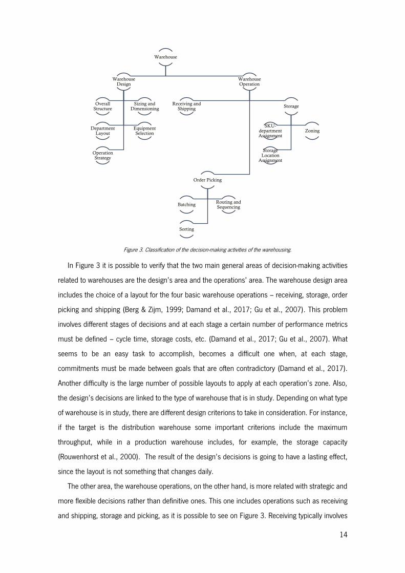
According to Gu et al. (2007), a simple scheme to classify both warehouse design and operation

planning problems is presented in Figure 3. This one summarizes the existing logistics’ decision-

making activities associated to warehouses.

14

Figure 3. Classification of the decision-making activities of the warehousing.

In Figure 3 it is possible to verify that the two main general areas of decision-making activities

related to warehouses are the design’s area and the operations’ area. The warehouse design area

includes the choice of a layout for the four basic warehouse operations – receiving, storage, order

picking and shipping (Berg & Zijm, 1999; Damand et al., 2017; Gu et al., 2007). This problem

involves different stages of decisions and at each stage a certain number of performance metrics

must be defined – cycle time, storage costs, etc. (Damand et al., 2017; Gu et al., 2007). What

seems to be an easy task to accomplish, becomes a difficult one when, at each stage,

commitments must be made between goals that are often contradictory (Damand et al., 2017).

Another difficulty is the large number of possible layouts to apply at each operation’s zone. Also,

the design’s decisions are linked to the type of warehouse that is in study. Depending on what type

of warehouse is in study, there are different design criterions to take in consideration. For instance,

if the target is the distribution warehouse some important criterions include the maximum

throughput, while in a production warehouse includes, for example, the storage capacity

(Rouwenhorst et al., 2000). The result of the design’s decisions is going to have a lasting effect,

since the layout is not something that changes daily.

The other area, the warehouse operations, on the other hand, is more related with strategic and

more flexible decisions rather than definitive ones. This one includes operations such as receiving

and shipping, storage and picking, as it is possible to see on Figure 3. Receiving typically involves

Warehouse

Warehouse Design

Overall Structure

Sizing and Dimensioning

Department Layout

Equipment Selection

Operation Strategy

Warehouse Operation

Receiving and Shipping

Storage

SKU-department Assignment

Zoning

Storage Location

Assignment

Order Picking

BatchingRouting and Sequencing

Sorting

15

the physical unloading of incoming transport and, in some cases, also includes activities such as

unpacking, and repackaging, and quality control (Berg & Zijm, 1999; Rushton et al., 2010). While

this operation brings products to the warehouse, there is the opposite one, the shipping, that loads

outbound vehicles making the products leave the warehouse.

Inside the warehouse, there are two main operations, the storage and the picking. In the storage

operation, products are usually taken to the storage area, which is, most of the cases, the largest

space user in many warehouses (Gu et al., 2007; Rushton et al., 2010). The order picking, or just

picking, is the operation of collecting a certain type and number of products before shipping, to

satisfy the customer’s request. About these two inside operations there is a high number of

problems to solve such as the picking routing, picking batching and sorting, the storage layout and

zoning, among others (Damand et al., 2017).

In this work, all the efforts of study are directed to the warehouse operation of receiving and

shipping. Inside this thematic there are a lot of specific problems that must be considered. Some

of these problems will be exemplified next, as well as the specification of which one is the target of

this dissertation.

2.3.2. Receiving and Shipping

Receiving and shipping are the interface of any warehouse for incoming and outgoing physical

flow. Incoming shipments are brought to the warehouse, unloaded at the receiving docks, and put

into storage (Rouwenhorst et al., 2000). Orders are picked from storage, prepared and shipped to

customers through shipping docks. Receiving and shipping operations involve, for example, the

assignment of trucks to docks and the scheduling of loading and unloading activities (Gu et al.,

2007; Rouwenhorst et al., 2000). Thus, associated to the operation of receiving and shipping there

are other specific problems. Among others, it is possible to differentiate three: the truck-dock

assignment; the order-truck assignment; and the truck dispatch schedule (Shipping) (Gu et al.,

2007).

So, with information about things such as the incoming shipments – arrival time and contents;

the customers’ demands – orders and their expected shipping time; and the warehouse dock layout

and available material handling resources (Gu et al., 2007), it is possible to make decisions about

what strategies to adopt to avoid costs and delays. In this sense, the basic decisions in

receiving/shipping operations can be summarized as:

16

(1) The assignment of inbound and outbound shippers – either client’s shippers or

supplier’s shippers – to docks, which determines the total internal material flows;

(2) The schedule of the service of shippers at each dock. Assuming a set of shippers is

assigned to a dock, the problem is like a machine scheduling problem, where the

arriving shippers are the jobs to be scheduled;

(3) The allocation and dispatching of material handling resources, such as labor and

material handling equipment (Gu et al., 2007; Rouwenhorst et al., 2000).

These decisions are usually subject to performance criteria and constraints such as:

• Resources required to complete all shipping/receiving operations;

• Levels of service, such as the total cycle time and the load/unload time for the shippers;

• Layout, or the relative location and arrangement of docks and storage departments;

• Management policies, e.g., one customer per shipping dock;

• Throughput requirements for all docks (Gu et al., 2007).

Considering the level of knowledge about the shipments, decision making in receiving and

shipping can be distinguished in three different problems (Gu et al., 2007):

(a) No knowledge, other than warehouse layout;

(b) Partial statistical knowledge of arriving and departing processes, such as the average

level of material flow from an incoming shipper to an outgoing shipper;

(c) Perfect knowledge of the content of each arriving shipper and each departing shipper

(Gu et al., 2007).

In the scenario (a), it is not possible to have any basis for assigning carriers to docks, as well

as it is not possible to precisely assign goods to storage locations. So, it is not clear in this case if

there is any storage assignment rule that fits better than others. Usually, public warehouses can

operate under this set of conditions, for example (Gu et al., 2007).

The second scenario is most common in company-owned or dedicated distribution warehouses

and is the basis for most of the decision models in the literature (Gu et al., 2007).

The third, and last, scenario is becoming increasingly common through the application of

advanced information technologies (Gu et al., 2007), as it is the one that aggregates all of the

information needed to make more precise decisions.

In this work the general problem in study is the one stated in the point (2) – the schedule of the

service of shippers at each dock, including the specific problems of dock-truck assignment and the

dispatch schedule. In fact, the problem consists of scheduling, and is solved as a machine

17

scheduling problem where the trucks/shippers are the jobs to be schedule. Also, the focus

operation is the shipping, not including the receiving. Also, the warehouse in study is a production

warehouse that is located outside the production line, so the final products enter the facility directly

from the production line.

In the next section the concepts about the machine scheduling problem are going to be

discussed to understand how this problem stated so far is going to be solved. In fact, there are two

ways to solve this problem, the exact method and the heuristic one. What these two ways mean

and what distinguish from one to another, are also the topics of the next section.

2.4. Scheduling

The problem in study is going to be treated as a Scheduling Problem, a Machine Scheduling

Problem. But, before the real problem description itself and the modeling, there is some

background that needs to be clarified.

Scheduling is a decision-making process that is used on a regular basis in many manufacturing

and service industries. It deals with the allocation of resources to tasks over given time periods and

its goal is to optimize one or more objectives (Pinedo, 2016c).

The resources and tasks in an organization can take many different forms. The resources may

be machines in a workshop, runways at an airport, crews at a construction site, processing units

in a computing environment, and so on. The tasks may be operations in a production process,

take-offs and landings at an airport, stages in a construction project, executions of computer

programs, and so on (Pinedo, 2016c). Taking in consideration this work, the resource is the

warehouse while the task is the allocation of the clients. Each task may have a certain priority level,

an earliest possible starting time and a due date. The objectives can also take many different forms.

One objective may be the minimization of the completion time of the last task and another may be

the minimization of the number of tasks completed after their respective due dates (Pinedo,

2016c).

About the scheduling of the shipping operation, very few formal models have been developed

for the management of shipping as well as the receiving operations. Most of the literature that is

available in this area addresses shipping and receiving operations and truck-to-dock assignment

strategies for cross-docking warehouses (Gu et al., 2007). However, this work is not about cross-

docking – considered a distribution warehouse – but instead, a production warehouse, as stated

18

so far. So, with this study the goal is also to address some research about this type of problems,

considering the lack of it in the current literature.

One thing that needs to be considered when discussing about scheduling is that the focus of

any scheduling problem is the efficient allocation of one or more resources to activities over time

(Chen, Potts, & Woeginger, 1998). Considering the Machine Scheduling Problem – a more specific

problem of scheduling –, originally found in the manufacturing systems, a job consists of one or

more activities, and a machine is a resource that can perform at least one activity at a time (Chen

et al., 1998). The number of jobs is denoted by n and the number of machines by m . Usually,

the subscript j refers to the job while the subscript i refers to the machine (Pinedo, 2016c).

The Machine Scheduling Problem that is consider for this problem can be described as follows:

there are m machines that are used to process n jobs. A schedule specifies, for each machine

( 1,..., )i i m= and each job ( 1,..., )j j n= , one, or more, time intervals throughout which

processing is performed on job j by the machine i (Brucker & Knust, 2012b; Chen et al., 1998).

A schedule is feasible if there is no overlapping of time intervals corresponding to the same job (so

that a job cannot be processed by two machines at once), and also if it satisfies various

requirements relating to the specific problem type. The problem type is specified by the machine

environment, the job characteristics and an optimality criterion (Chen et al., 1998).

2.4.1. Machine Environment

Different configurations of machines are possible. An operation refers to a specific period of

processing by some machine type. It is possible to assume that all machines become available to

process jobs at time zero (Chen et al., 1998).

In a single-stage production system, each job requires one operation, whereas in multi-stage

systems the jobs require operations at different stages. Single-stage systems involve either a single

machine, or m machines operating in parallel. The case of a single machine is the simplest of all

possible machine environments and is a special case of all other more complicated machine

environments (Brucker & Knust, 2012b; Pinedo, 2016b). In the case of parallel machines three

general cases can occur: identical parallel machines in which the processing time of job j does

not depend on the machine performing the job; uniform parallel machines in which the machines

operate at different speeds but are otherwise identical; and unrelated parallel machines – the

19

opposite of identical parallel machines, – in which the processing time of a job j depends on the

machine assignment (Brucker & Knust, 2012b; Chen et al., 1998; Pinedo, 2016b).

Regarding the multi-stage systems, or so-called shop scheduling problems (Brucker & Knust,

2012b), there are three main types to take in consideration. All such systems that are going to be

consider comprise S stages, each having a different function. In a flow shop with S stages, the

processing of each job goes through the stages 1,..., s in that order (Brucker & Knust, 2012b;

Chen et al., 1998). In an open shop, the processing of each job also goes once through each stage,

but the routing (that specifies the sequence of stages through which a job must pass) can differ

between jobs and forms part of the decision process (Chen et al., 1998). In a job shop, each job

has a given routing through the stages – specific precedencies, and the routing may differ from job

to job (Brucker & Knust, 2012b; Chen et al., 1998). There are also multiprocessor variants of multi-

stage systems, where each stage comprises several (usually identical) parallel machines (Chen et

al., 1998), becoming flexible job shop and flexible flow shop (Pinedo, 2016b).

Furthermore, a machine may be able to process several jobs, say b , simultaneously; that is, it

can process a batch of up to b jobs at the same time. In this context, the motivation for batching

jobs is in the increase of efficiency since it may be cheaper or faster to process jobs in a batch

than to process them individually (Potts & Kovalyov, 2000).The processing times of the jobs in a

batch may not be all the same and the entire batch is finished only when the last job of the batch

has been completed (Pinedo, 2016b). The definition of a batch is given as follows. The jobs are

supposed to be partitioned into F families, 1F . A group of jobs belongs to the same family

according to their similarity, so that no setup is required for a job if it belongs to the same family

of the previously processed job (Potts & Kovalyov, 2000). Hereupon, a batch is defined as a set of

jobs of the same family. While families are supposed to be given in advance, batch formation is a

part of the decision-making process (Allahverdi, Ng, Cheng, & Kovalyov, 2008).

In addition, two types of batching machines are categorized in the literature: the serial batching

machine and the parallel batching machine. On a serial batching machine, the length of a batch

equals the sum of the processing times of its jobs (Baptiste, 2000). While on a parallel batching

machine, the length of a batch equals the largest processing time of its jobs (Baptiste, 2000).

Batching models are further partitioned into batch availability and job availability models.

According to the batch availability model, all the jobs of the same batch become available for

processing and leave the machine together (Allahverdi et al., 2008; Potts & Kovalyov, 2000). For

example, this situation is very common to occur if the jobs in a batch are placed on a pallet. In

20

these cases, the pallet is only moved from the machine when all these jobs are processed. An

alternative assumption is the job availability model, in which each job’s start and completion times

are independent of other jobs in its batch (Allahverdi et al., 2008; Potts & Kovalyov, 2000).

2.4.2. Job Characteristics

The processing requirements of each job j are given: for the case of a single machine and

identical parallel machines, jp is the processing time; for uniform parallel machines, the

processing time on machine i may be expressed as /j ip s where is is the speed of machine i ;

for the case of unrelated parallel machines, a flow shop and an open shop, ijp is the processing

time on machine/stage i ; and for a job shop, ijp denotes the processing time of the ith operation

(which is not necessarily performed at stage i ). It is possible to assume that all jp and ijp are

non-negative integers (Chen et al., 1998).

In addition to its processing requirements, a job is also characterized by its availability for

processing, any dependence on other jobs, and whether interruptions in the processing of its

operations are allowed (Chen et al., 1998; Meiswinkel, 2018). The availability of each job j may

be restricted by its integer release date jr that defines when it becomes available for processing,

and/or by its integer due date jd that represents the completion date. Completion of a job after

its due date is allowed, but then a penalty is incurred. When a due date must be met it is referred

to as deadline and denoted by jd (Chen et al., 1998; Meiswinkel, 2018; Pinedo, 2016b).

Job dependence arises when there are precedence constraints on the jobs. If job j has

precedence over job k , then k cannot start its processing until j is completed. Precedence

constraints are usually specified by a directed acyclic precedence graph G with vertices 1,...,n .

There is a directed path from vertex j to vertex k if and only if job j has precedence over job k

(Chen et al., 1998; Pinedo, 2016b). Some scheduling models allow preemption: the processing of

any operation may be interrupted and resumed at a later time on the same or on a different

machine (Chen et al., 1998).

21

2.4.3. Optimality Criterion

Given a schedule , it is possible to calculate for job j : the completion time jC ; the flow time

j j jF C r= − ; the lateness j j jL C d= − ; the earliness max ,0j j jE d C= − ; the tardiness

max ,0j j jT C d= − ; and the unit penalty 1jU = if j jC d , and 0jU = otherwise (Chen et

al., 1998).

Some commonly used optimality criteria involve the minimization of the maximum completion

time, or makespan, max max jC C= – a minimum makespan usually means a good utilization of

the machine(s); the maximum lateness max max jL L= – it measures the worst violation of the

due dates; the maximum cost max max if f= , and the maximum earliness max max jE E= (Chen

et al., 1998; Meiswinkel, 2018; Pinedo, 2016b).

In case of weighted criterions, where the weight measures the importance of the job, some

commonly used criterions are the total weighted completion time ( )j j

j

w C ; the total weighted

flow time ( )j j

j

w F ; the total weighted earliness ( )j j

j

w E ; the total weighted tardiness

( )j j

j

w T ; the weighted number of late jobs ( )j j

j

w U ; or the total cost j

j

f , where each

maximization and each summation is taken over all jobs j (Chen et al., 1998; Meiswinkel, 2018).

Some situations require more than one of these criteria to be considered (Chen et al., 1998;

Pinedo, 2016b).

2.4.4. Three-Field Representation

Considering all these aspects, a representation is needed to define any machine scheduling

problem. So, it is convenient to adopt the representation scheme of (Graham, Lawler, Lenstra, &

Kan, 1979). This is a three-field descriptor | | which specifies the problem type where

represents the machine environment, defines the job characteristics, and is the optimality

criterion (Allahverdi et al., 2008; Chen et al., 1998; Meiswinkel, 2018).

For there is a possibility of combinations that can occur. This field takes the form

1 2 3 = , where 1 , 2 and 3 are interpreted as follows. If 1 = , it means the problem

deals with a single machine; if 1 P = : identical parallel machines; and if 1 Q = , R ,O , F or

22

J uniform parallel machines, unrelated parallel machines, an open shop, a flow shop or a job

shop, respectively (Chen et al., 1998; Meiswinkel, 2018).

For the 2 field there are only three different possibilities: if 2 = the number of

machines/stages is arbitrary; if 2 m = it means that there is a fixed number m of machines;

and last if 2 s = that means that there is a fixed number s of stages. Finally, the 3 element

only exists if there are any stages on the process (Chen et al., 1998; Meiswinkel, 2018).

So, to conclude and taking into example a single machine problem, the 1 2 3 = would be

represented as 1 = , or simply 1 = (Chen et al., 1998).

The second field 1 2 3 4 5 6 7, , , , , , indicates job characteristics. Excluding the

1 , that is related to the on-line concepts and on-list, typically all the other ones are characterized

when describing a problem. Saying so, the other fields are described as follows: 2 , jr and

defines the existence or not of the release dates, if jobs have release dates than 2 jr = . On the

other hand, 3 is destined to characterize the existence or not of the deadlines, following the same

example of 2 . That said, 3 , jd , and in case of specific deadlines: 3 jd = . The 4

factor defines the existence or not of preemption. So, 4 , pmtn and if preemption is allowed,

4 pmtn = (Chen et al., 1998; Meiswinkel, 2018).

The two parameters – 5 6, – are the ones related to precedencies and processing times,

respectively. In terms of precedencies, 5 = if there is not any precedence constraint specified.

In the case of specific precedencies 5 can be equal to chain, intree, outtree, tree or prec. The

meaning of each possibility is related to the way precedencies are defined. For example, in the

case of 5 prec = it means that jobs have arbitrary precedence constraints (Allahverdi et al.,

2008; Chen et al., 1998).

The processing times identified by 6 , can be equal to one out of three different ways. Saying

so, 6 , 1, 1j ijp p = = , where 6 = means that processing times are arbitrary;

6 1jp = = means that all jobs in a single-stage system have unit processing times (Chen et al.,

23

1998; Meiswinkel, 2018); and finally 6 1ijp = = means that all operations in a multi-stage

system have unit processing times (Chen et al., 1998).

The 7 defines the existence, or not, of batching scheduling. A machine may be able to process

several jobs, say b , simultaneously; that is, it can process a batch of up to b jobs at the same time

(Pinedo, 2016b). There three alternative values for 7 (Dürr, Knust, Prot, & Vásquez, 2016).

7 s batch = − , the batching machine is a serial batching machine which means that the

processing time of a batch is the total processing time over all jobs in the batch (Baptiste & Jouglet,

2001; Dürr et al., 2016). 7 ( )batch = , the machine is a parallel batch machine and there is

no limit on the number of jobs in a batch and the processing time of a batch is the maximum

processing time over all jobs in the batch (Dürr et al., 2016; Potts & Kovalyov, 2000). Last,

7 ( )batch b = , the batching machine is a parallel batch machine and the batch consists of a

maximum b jobs and its processing time is the maximum processing time over all jobs in the batch

(Brucker et al., 1998; Dürr et al., 2016).

Lastly, the third field defines the optimality criterion, which involves the minimization of

max ,C max ,L max ,E max ,T max ,f ( ) ,j jw C ( ) ,j jw F ( ) ,j jw E ( ) ,j jw T

( ) ,j jw U jf (Allahverdi et al., 2008; Chen et al., 1998; Meiswinkel, 2018). As it was

being said lately, it is sometimes appropriate to consider several of these criteria.

To finish this section and to illustrate the three-field descriptor, three examples are now

presented: the 1| , |j j jr prec w C is the problem of scheduling jobs with release dates and

precedence constraints on a single machine to minimize the total weighted completion time. The

max| |R pmtn L is the problem of preemptively scheduling jobs on an arbitrary number of

unrelated parallel machines to minimize the maximum lateness (Chen et al., 1998). And finally,

the third example, | , |m j j j jP r d w T (Pinedo, 2016b) refers to a system with m machines in

parallel; job j arrives at release date jr and has to leave by the due date jd . If job j is not

completed in time a penalty j jw T is incurred.

24

2.5. Methodologies

After understanding how the machine scheduling problem is characterized and defined, in this

section, the main goal is to outline the methods and techniques that are used to analyze and solve

scheduling problems.

In fact, a scheduling problem is not more than a special type of combinatorial optimization

problem. Thus, it is possible to use methodologies already used for combinatorial optimization

(Chen et al., 1998). In this sense, a significant research topic in scheduling as well as in

combinatorial optimization is the use of Complexity Theory to classify scheduling problems as

polynomial solvable or NP-hard.

About the complexity theory, generically it is a central field of the theoretical foundations of

Computer Science. This field is concerned with the study of the intrinsic complexity of

computational tasks. Therefore, a typical complexity theoretic study refers to the computational

resources required to solve a computational task. Thus, computational complexity is the general

study of what can be achieved within limited time and/or other limited natural computational

resources (Goldreich, 2008).

About this matter, practical experience has shown that some scheduling problems are easier to

solve than others. For example, computers of today can solve instances of problem 1 | | j jw C

with several thousands of jobs within seconds, whereas it takes at least several hours to solve some

even moderately sized instances of problem max | | CJ with, for example, 30 jobs and 30 machines

(Chen et al., 1998). So, in this sense, computational complexity theory provides a mathematical

framework that is able to explain these “observations from practice” and that yields a classification

of problems into easy and hard ones (Chen et al., 1998; Dorigo & Stützle, 2003). This

mathematical framework is not relevant for this study so, about this matter the goal is only to

understand that some problems are not easy to solve, even for computers, therefore sometimes it

is necessary to have some techniques to overcome these difficulties. But, before the analysis of

these techniques, it is important to distinguish the easy from the hard problems, even if in general

aspects.

Let us start with a definition of an algorithm. An algorithm is a step-by-step procedure for solving

a computational problem. For a given input x , it generates the correct output ( )f x after a finite

number of steps. The efficiency of an algorithm for a given problem is measured by the maximum

25

number of computational steps and time needed to obtain an optimal solution as a function of the

size of the instance (Chen et al., 1998; Pinedo, 2016a).

This, in turn, requires a definition of a computational step. In practice, a computational step in

an algorithm is either a comparison, a multiplication or any data manipulation step concerning one

job (Pinedo, 2016a). The efficiency of an algorithm is then measured by the maximum number of

computational steps needed to obtain an optimal solution (as a function of the size of the instance,

i.e., the number of jobs). The number of computational steps may often be just the maximum of

iterations the algorithm has to go through. Even if this number of iterations is typically approximated

(Chen et al., 1998; Pinedo, 2016a).

In this sense, a problem is said to be polynomial if its time complexity is bounded by a

polynomial input size (Chen et al., 1998); on the other hand, if that polynomial time is not verified,

the problem is said to be NP-hard. The NP-hardness of a problem suggests that there are instances

for which the computational time required to find an optimal solution increases exponentially with

problem size. So, for NP-hard problems, what seems to happen is that it is not always possible to

find an optimal solution quickly.

So, if large computational times for such problems are unacceptable, then, instead of searching

for an optimal solution with enormous computational effort, a heuristic (method) or an

approximation algorithm is used to give an approximate solution (Chen et al., 1998; Pinedo,

2016c).

In addition to exact methods for small instances, to obtain exact solutions of NP-hard scheduling

problems, enumerative algorithms are usually applied. The main types of enumerative algorithms

are branch and bound and dynamic programming, and both may benefit from dominance rules

which help to restrict the search (Chen et al., 1998; Pinedo, 2016d). For many scheduling

problems, metaheuristic methods including simulated annealing, greedy randomized adaptive

search, tabu search and genetic algorithms are very successful in generating high-quality solutions

(Berghman & Leus, 2015; Chen et al., 1998; Damodaran, Ghrayeb, & Guttikonda, 2013; Kadhim,

Ali, & Kassim, 2018).

Resuming all these ideas, the main tools for providing negative results – meaning the non-

existence of fast algorithms for a specific problem, – come from computational complexity theory.

Also, the main tools for providing positive results are exact methods and enumerative algorithms

for finding exact solutions and heuristic methods for finding approximate solutions. For this work

26

the tools used for providing solutions were an exact method and two heuristic methods. Therefore,

in the next sections these two subjects are going to be contextualized.

2.5.1. Mathematical Model

To solve a problem with exact methods, a mathematical model is usually developed. This in

turn, when associated to optimization problems may become a linear programming model, if the

function to minimize, as well as its constraints, are linear.

The linear programming subject is mainly concerned with the optimization – minimization or

maximization – of a linear function, always having in consideration a set of linear equality and/or

inequality constraints or restrictions (Bazaraa, Jarvis, & Sherali, 2010). Therefore, it is possible to

condense the structure that characterizes a linear programming problem into the following form

(Bazaraa et al., 2010; Lewis, 2008; Taha, 2007; Vanderbei, 2014):

In a more mathematical approach, it is possible to summarize a linear programming model in

the following notation (Bazaraa et al., 2010; Lewis, 2008; Vanderbei, 2014):

1 1 2 2Minimize ... n nc x c x c x z+ + + =

11 1 12 2 1 1

21 1 22 2 2 2

Subject to a ...

a ...

n n

n n

x a x a x b

x a x a x b

+ + +

+ + +

1 1 2 2

1 2

a ...

, , ..., 0.

m m mn n m

n

x a x a x b

x x x

+ + +

Note that in this case the constraints considered are inequalities ( ), but they can be either

equalities or inequalities. The next relation sums up this idea (Vanderbei, 2014):

1 1 2 2 ... n na x a x a x b

+ + + =

So, and subtitling the notation presented so far, in linear programming, z , the expression being

optimized, is called the objective function. Plus, the variables 1 2, ,..., nx x x are called decision

variables, the ones to be determined (Bazaraa et al., 2010; Lewis, 2008). Last, but not least, the

max or min Objective Function

subject to Constraints

27

coefficients 1 2, ,..., nc c c are known as cost coefficients and the coefficients ija for 1,...,i m= ;

1,...,j n= are called the technological coefficients (Bazaraa et al., 2010).

Any solution of the model is feasible if it satisfies all the constraints (Lewis, 2008; Taha, 2007).

However, it is only optimal if, in addition to being feasible, it yields the best – maximum or minimum

– value of the objective function (Taha, 2007). However, even if linear programming models are

designed to "optimize" a specific objective criterion subject to a set of constraints and can achieve

in fact the best solution, that does not ensure the quality of the resulting solution for the practical

problem. In fact, the quality highly depends on the capacity of the model in representing the real

system (Taha, 2007).

The linear programming model becomes an Integer Linear Programming (ILP) model if all the

variables are restricted to be integers. If the optimization problem involves continuous and integer

variables, then the linear programming model becomes a Mixed Integer Linear Programming

(MILP) model (Pochet & Wolsey, 2006).

Considering the amount of constraints and variables and the length of the input information, a

computer solver is going to be used to solve the MILP model. To have access to commercial solvers,

internet platforms are usually used, one example is the NEOS Server. The NEOS Server is a free

internet-based service for solving numerical optimization problems (Wisconsin Institutes for

Discovery, 2018). Hosted by the Wisconsin Institute for Discovery at the University of Wisconsin in

Madison, the NEOS Server provides access to more than 60 state-of-the-art solvers in more than a

dozen optimization categories (Wisconsin Institutes for Discovery, 2018), for academic and

scientific purposes. To submit a model – usually named job – in the NEOS Server, a modeling

language is needed. In this sense, one example of a modeling language is the AMPL – A

Mathematical Programming Language. AMPL closely resembles the symbolic algebraic notation,

already mentioned, that many modelers use to describe mathematical programs (Fourer, Gay, &

Kernighan, 1990). Still, it is regular and formal enough to be processed by a computer system

(Fourer et al., 1990).

While AMPL creates optimization problems from models and data, and retrieves results for

analysis, solvers are the number-processing algorithms that compute optimal solutions (AMPL

Optimization Inc., 2018). There are several solvers that can solve specific linear optimization

problems, the so called LP-solvers (Meindl & Templ, 2013). Available LP-solvers differ in many

ways. They come with different licenses and features, for instance, different solvers may contrast

in terms of how problems can be specified (Meindl & Templ, 2013). Among the most popular

28

solvers is the Gurobi. Since it is beyond the scope of this project to enumerate more solvers and

describe them, the Gurobi was the one being used to solve the mathematical model. Saying so,

and just briefly presenting this solver, the Gurobi Optimizer is seen as a modern solver for linear

as well as other related (non-linear, e.g.) mathematical optimization problems (Meindl & Templ,

2013).

2.5.2. Heuristic Methods

The knowledge that a scheduling problem is considered NP-hard brings no consolation when

the goal is to solve the problem. Therefore, after understanding how mathematical models can be

modeled and processed, to obtain both feasible and optimal solutions, it is now time to realize how

these mathematical models can be “transformed” into approximate algorithms. Often, approximate

algorithms are the only feasible way to obtain near optimal solutions at relatively low computational

cost (Dorigo & Stützle, 2003). However, there is not any recipe to turn a mathematical model in

an approximation algorithm so, in this case the word “transform” is used in a figurative way. In

fact, “transform” in this case only means to create an algorithm capable to incorporate the

objective function and all its constraints but, without needing to cover all the feasible solutions that

an exact algorithm usually covers (Brucker, 2004b).

Heuristic algorithms are often applied to determine solutions that hopefully are not too far away

from the global optimum (Brucker, Hurink, & Werner, 1997). Among the reasons that justify the

large utilization of heuristics in operations research, it is possible to highlight the fast results

(Brucker, 2004b; Silver, 2002). However, even if the main usage of the word “heuristic” is mostly

the adjective of “improving problem solving”, there might also be a slightly negative meaning

attached to it (Groner & Groner, 1983). In fact, between the main disadvantages of a heuristic

method is the lack of a good solution guarantee (Brucker, 2004b; Groner & Groner, 1983). That

happens because the quality of a solution is directly attached to the quality of the heuristic’s

method. So even if the modern picture of a search for the solution is intelligently directed, there is

still an inherent uncertainty (Aickelin & Clark, 2011; Groner & Groner, 1983). Thus, giving this

context, a possible generic definition associated to the concept of heuristic might simply be any

approach without formal guarantee of performance (Brucker, 2004b).

Most heuristic algorithms used are either constructive algorithms or local search algorithms

(Dorigo & Stützle, 2003). However, these two types of methods are significantly different.

Considering the constructive algorithms, these type of heuristic algorithms build solutions in an

29

incremental way starting with an empty initial solution and iteratively adding appropriate solution

components without backtracking until a complete solution is obtained (Dorigo & Stützle, 2003).

For example, the construction of a first solution following a simple rule such as the Earliest Due

Date (EDD) is a constructive algorithm. The main advantage of constructive algorithms is that they

are typically the fastest approximate methods (Dorigo & Stützle, 2003). However, the solutions

they generate are not of a very high quality and they are not guaranteed to be optimal with respect

to small changes (Dorigo & Stützle, 2003). Giving this first solution for a problem a constructive

algorithm provides, another common heuristics that arises and, one of the most successful

methods for getting rid of hard combinatorial optimization problems is the discrete equivalent of

"hill climbing", currently known as local (or neighborhood) search (Brucker, 2004b; Brucker et al.,

1997; Brucker & Knust, 2012a; Dorigo & Stützle, 2003).

Local search is an iterative procedure which moves from one solution to another as long as

necessary (Brucker, 2004b). The procedure of a typical local search algorithm is to explore the

search space of complete solutions, in order to find better feasible solutions (Dorigo & Stützle,

2003). The search space is known as neighborhood structure. To implement local search it is

necessary to define a base solution and a neighborhood structure (Brucker & Knust, 2012a; Dorigo

& Stützle, 2003; Sampson & Weiss, 1993). To create the neighborhood structure a certain move,

or more than one, are applied to a given solution. The quality of the final solution achieved is

directly related to the moves applied to obtain the final neighborhood structure. So, it is possible

to conclude that the choice of a suitable structure has some important influence on the quality of

the search algorithm (Brucker et al., 1997; Dorigo & Stützle, 2003; Sampson & Weiss, 1993). In

sum, a local search procedure can be defined by the next four steps (Sampson & Weiss, 1993):

(1) The construction of a primary solution as the base solution, using arbitrary methods or

constructive algorithms, for example;

(2) The changing of the base solution accordingly to the neighborhood structure;

(3) If the changed solution provides a better objective function value than the base solution,

then the changed solution becomes the base solution;

(4) Start again at step 2 until no improving neighbor solution can be found.

Usually these steps are repeated until no improving neighbor solution can be found in the

neighborhood of the current solution and the algorithm ends in a local optimum (Dorigo & Stützle,

2003).

30

Besides constructive algorithms and local search, another type of heuristic method is the

metaheuristics. Metaheuristics are powerful algorithmic approaches which have been applied with

great success to many difficult combinatorial optimization problems. An advantage of

metaheuristics is that they can easily handle the complicating constraints found in real-life

applications (Gendreau & Potvin, 2005).

In the term metaheuristics, first introduced by (Glover, 1986), the prefix meta- means “beyond”

or “higher level.” This type of heuristic algorithms usually perform better than simple heuristics

(Dorigo & Stützle, 2003; Gandomi, Yang, Talatahari, & Alavi, 2013; Yang, 2011). All metaheuristic

algorithms use some trade-off of local search and global exploration. The variety of solutions is

often realized via randomization (Gandomi et al., 2013). What this randomization is good for is to

provide a method to move away from local search and instead look for a more global scale search

(Gandomi et al., 2013).

The main components of any metaheuristic algorithm are: intensification and diversification, or

exploitation and exploration (Blum & Roli, 2003). Diversification means generating diverse solutions

so as to explore the search space on the global scale (Gandomi et al., 2013). On the other hand,

intensification means focusing on the search in a local region by exploiting the information that a

current good solution is found in this region (Gandomi et al., 2013; Yang, 2011). The diversification

via randomization increases the diversity of the solutions while keeping the solutions from being

stuck at local optima. The good combination of these two major components will usually ensure

that the global solution is achievable (Gandomi et al., 2013).

Summarizing and concluding metaheuristic’s topic, it is possible to outline some fundamental

characteristics, being them (Blum & Roli, 2003; Gandomi et al., 2013; Osman & Laporte, 1996):

• Metaheuristics are strategies that “guide” the search process;

• Techniques which constitute metaheuristic algorithms range from simple local search

procedures to complex learning processes;

• Metaheuristics are approximate and usually non-deterministic;

• Metaheuristic algorithms may incorporate mechanisms to avoid getting trapped in

confined areas of the search space;

• Today’s more advanced metaheuristics use search experience (using memory) to guide

the search.

To conclude this section, it is relevant to notice that when evolving from construction algorithms,

to local search and lately to metaheuristics, the level of complexity and the time needed to solve

31

the problem grows. On the other hand, it is likely to find a better solution using a metaheuristic

than a construction algorithm. Nevertheless, any heuristic algorithm is usually (or always), faster

than a mathematical program, or exact method, because, as it was already mentioned, heuristic

methods do not cover all feasible solutions. When solving a problem, it is important for the expert

to analyze all the possibilities of resolutions in order to find the one that generates good solutions

with the lesser number of resources needed.

33

3. Problem Description

The problem in study arises in the cement industry. To begin this new chapter, a global overview

of this industry is going to be presented. After this, the real problem itself is going to be descripted

and some assumptions will be established. Finally, before ending this chapter, three different ways

for formulating the problem will be presented, however, only one of them is going to be extended

for the chapter 4 – The Methodology. These three ways are different because some problem

specifications differ from one to another. The one that is going to be adopted to solve the problem,

is the one that best approaches the formulation of the problem from the reality.

3.1. Cement Industry – Global Overview

Cement being the second most consumed substance in the world, after water, is an

irreplaceable ingredient in a vast majority of applications (Amrina & Vilsi, 2015; Noche & Elhasia,

2013). It is the glue of concrete and the most massive manufactured product by human society

with the largest materials flow in the world and the basic ingredient for the construction industry

(Elhasia, Noche, & Zhao, 2013; Selim & Salem, 2010; Shen et al., 2017). For instance,

constructions such as civil infrastructure projects, houses, power generation plants and many more

cannot be built without cement (Noche & Elhasia, 2013).

The consumption of cement, in return, is closely linked to both the state of economic

development in any given country or region and to the economic cycle (Noche & Elhasia, 2013).

In some more developed markets the cement sales are dependent on the growth and habits in the

construction sector, a sector that is itself following very closely the economic situation prevailing

(Noche & Elhasia, 2013). The fast industrialization and urbanization of the current world calls for

more and more infrastructures, highways, rail ways, and being cement the main construction

material, the demand of this product keeps increasing quickly (Shen et al., 2017). So, allied to

both economic and population growth (Roser, 2018; Roser & Ortiz-Ospina, 2018), the production

of cement worldwide is growing too, as it is possible to verify in the Figure 4.

34

Figure 4. World cement production over the past 10 years. Data source: (USGS, 2018) - Cement Statistics and Information.

Even if this growth of the cement production is a good sign for companies in this sector, because

the demand is getting bigger, there are still many challenges to overcome. Sustainable

manufacturing, for instance, is certainly one of the critical issues for the cement industry (Amrina

& Vilsi, 2015; Selim & Salem, 2010). Sustainable manufacturing, on the other hand, can be defined

as the creation of manufactured products that minimize negative environmental impacts, preserve

energy and natural resources, are safe for employees, communities and consumers (Amrina &

Vilsi, 2015). The general principle of sustainable manufacturing is to reduce the intensity of

materials use, energy consumption and emissions, while maintaining, or improving, the value of

products to society and to organizations (Amrina & Vilsi, 2015).

Besides the sustainability, studies reflect that the two other major concerns of the cement

industry include the manufacturing process itself and the cement material management (Agudelo,

2009; Elhasia et al., 2013). While the manufacturing process does not match the scope of this

project, the cement material management on the other hand can clearly be included in the supply

chain management and the logistics of the cement industry (Agudelo, 2009). However, it is only a

part of the SCM which for itself is already a topic with limited research in the cement industry. In

the meantime, while topics such as distribution and transportation are also addressed in the

current literature (Agudelo, 2009), there is not much information about them (Elhasia et al., 2013;

Fonseca et al., 2018). With this work the aim is also to address more information concerning the

supply chain management in the cement industry, specifically in what concerns the distribution

process. A simple scheme that can illustrate the cement supply chain is evidenced in the Figure

5.

26062900 2825

33113597

38004080 4180 4100 4102 4128

0

500

1000

1500

2000

2500

3000

3500

4000

4500

5000

2007 2008 2009 2010 2011 2012 2013 2014 2015 2016 2017CEM

ENT

PR

OD

UC

TIO

N (

MIL

LIO

N T

ON

)

YEAR

35

Figure 5. Cement supply chain scheme.

The first operation of the cement supply chain includes the purchase and storage of raw

materials. Cement plants are frequently located near the quarries which are the source of their

main raw materials (Agudelo, 2009). After the manufacturing process, the cement is moved to

storage silos. Then, two things can happen because of the cement as a final product being sold

both as a bulk product or in bags. In the first situation the cement reaches the final client, through

bulk trucks, and in the second one the cement is bagged and lately storage until a customer places

an order.

The distribution process in the cement supply chain shows up in both bulk and bag cement

delivery and there are physical characteristics about the cement that challenge this distribution

process (Agudelo, 2009). Besides the fact that cement is a heavy and bulky load, which hinders

the process of moving the cement, it also has low-cost prices (Agudelo, 2009; Rushton et al.,

2010). Among others, these are the characteristics that make the relative costs of cement’s

logistics very high (Rushton et al., 2010). So, with certain improvements on the cement distribution

operations, costs can be reduced, service levels improved and, consequently, a more sustainable

industry might be achieved.

3.2. The case study

The case study of this work is inserted in the UH4SP project. The UH4SP was born in a

Portuguese company that provides a management software for other companies. In this case,

these other companies are, mostly, cement ones. In a typical cement plant, the cement

manufacturing facility is linked to the distribution one. After the operation of processing the cement,

this one is stored in silos or bagged and then stored in a distribution warehouse. However, it is also

frequent to have cement plants that do not include the manufacturing facility. These ones usually

36

only contain cement silos and distribution warehouses of bagged cement. In this specific case of

no manufacturing plants the only purpose of the plant is the distribution operations. Despite the

fact of the existence or not of the manufacturing facility, the distribution process in cement plants

always exist.

Regarding the current state of the processes that appears in every plant of the cement industries

in study, there are usually five steps. First, when a client arrives to the cement facilities he needs

to check in. Next, he will wait for being called to enter, in the parking lot. After waiting he will enter

through, usually, one of two different entries. In one of them there is the process of weighing and

in the other one there is not. Usually the clients that do not need to be weighed are the bulk trucks.

All the others, both to enter and to leave the cement plant, must be weighed, for control and

security purposes. Following the entry on the facility the client is going to drive to the place that

brought him to the cement plant. If he wants bagged cement he is going to the warehouse, if he

wants bulk cement then he is going to the cement silos and, finally, if he is not a client but else a

provider, he is going to the raw material warehouse to leave the products. Concluding his specific

process, the client is finally ready to leave the cement facility.

For this work the only clients that are going to be scheduled are the ones that request bagged

cement, since the distribution process in study is the distribution of bagged cement. In the next

section this distribution process is going to be descripted, as well as what are the real problems

that are happening that are causing troubles to both the cement company and its clients.

3.2.1. Cement Storage System

In the cement plants in study, the warehouses work as distribution centers. They store the

bagged cement and the customers go directly to the warehouse’s facility to pick their order, by

truck. For each warehouse there is a certain number of docking bays. A docking bay is a limited

space of the warehouse where the client’s truck can stop to load its order. An order is fulfilled only

through the companies’ resources. They might be manpower or other type of material handling

equipment such as forklifts. They usually are forklifts. The number of resources is equivalent to the

loading rate at each moment. The more resources exist, the faster is the loading process. On the

other hand, the number of docking bays of each warehouse is equivalent to its length. Usually the

length of the warehouse does not follow the number of resources available. So, if a certain

warehouse has a bigger length than another, that does not mean it has more resources.

37

These two characteristics – the length and the number of resources – of the warehouses are

the most important for this problem in study. Of course, there are other specifications such as the

level of stock of the warehouse, however, in this specific case study the level of stock is given as

being always enough to fulfill all the demand.

Giving this background, the main question now relies on what is happening in the reality that

causes trouble to both the cement company and its clients. The problem is primarily in the lack of

information and organization through all the supply chain. Allied to this, there is the nonexistence

of specific priority dispatching rules for the process of scheduling the clients/trucks. The

combination of these problems brings nothing but long queues in the parking lot, delays and

inefficient use of the resources. For example, with no scheduling models and with the lack of

information through the different entities in the supply chain, what happens is that sometimes there

is an opportunity to fulfill an order but there is not any information that both the resource of the

warehouse and the docking bay is available. On the other hand, in some cases what happens is

that for not knowing if there is not any docking bay or resource available the trucks start entering

the facility and are directed to the warehouse. When they arrive at the warehouse they realize it is

full and must wait in the roads of the cement plant causing congestions and consequently delaying

other clients that must use that road.

With all these problems a necessity of improvement and optimization arises. Considering this

conclusion, a scheduling model appears to be a good solution to work around these problems. In

fact, besides the necessity to promote the trade of information through the supply chain, a

scheduling procedure is also necessary to overcome problems such as inefficient use of resources

and the delays. In the next section some specifications and assumptions will be stablished to create

a scheduling model capable of solving most of the problems already mentioned.

3.2.2. Problem Specifications

Before initializing the process of scheduling the clients to the warehouse some assumptions

were established. First, a warehouse is seen as a set of four main characteristics. These ones are

the number of docking bays, the number of resources and the number and type of different

products available and their positions relatively to the docking bays of the warehouse – which will

directly interfere with the loading rate at each docking bay. The docking bays might be closer to a

certain type of product and distant from another. That means that the products are spread through

the warehouse but grouped per type of product. This implies that, when choosing the docking bay

38

that each client must go, it will be better to choose the one that is closer to the product demanded.

That way the loading rate will be greater. In addition, in some warehouses, several forklift trucks

move the pallets and place them inside the trucks. In other ones, depending on the country and

level of technology, rather than forklift trucks, it is the workers that move the cement bags and

place them inside the costumer’s trucks. In this study the only warehouses considered are the

ones whose resources are forklift trucks. However, the only thing that changes in these two different

scenarios is the loading rate. The loading rate is measured in number of material transported per

unit of time. If the warehouse’s resource is a forklift, this rate is going to be bigger than the case

where the warehouse’s resource is a worker. Besides, there is one more characteristic about the

forklifts that is important to considerate. In some warehouses the operation of loading one truck

can be done by more than one forklift. It is important to have this in consideration because it will

interfere with the loading rate. If two forklift trucks are loading one truck in simultaneously then the

loading rate is bigger than in the case where there is only one forklift. This is another technical

feature of the warehouse because it will differ from one to another. In some warehouses it will be

possible to have one truck being loaded by more than one resource and in others it will not.

Besides these characteristics of the warehouses there are the ones about the clients. Globally,

the clients are characterized by the type and the quantity of product they order, their release dates

and due dates. With this information and the information about the warehouse, it is possible to

build a schedule capable of satisfying both the costumers and company restrictions. This schedule

will also add more organization to the cement plant and, also, possibly reduce delays and the

waiting time in the parking lot. Also, with the entire knowledge of where the costumers at each time

of the process are and what resources are being used, it will be possible to improve the efficiency

of the resources themselves. The case where it would not be possible to know if a resource was

available to be use, with the scheduling model, hopefully, will not happen again.

In the next section three different ways to solve this scheduling problem will be exposed. In the

end only one of them will be used. However, it is important to notice that all the three can be used

depending of the technical features of the warehouses in study.

3.3. Problem Formulation

Three main different warehouse configurations were distinguish considering the range of

cement industries in study. In the first one, the warehouse has more than one docking bay but only

39

one forklift truck. In the second configuration the warehouse has equally more than one docking

bay but in this case it has more than one forklift truck but less than the number of docking bays.

In the third and last configuration the number of docking bays and the number of forklifts are the

same and more than one. Different configurations ask for different ways of solving the problem.

Therefore, if the warehouse has only one forklift truck it can be solve as a single machine scheduling

problem, if it has more than one forklift but less than the number of docking bays it can be solve

as a batch scheduling processing problem and, last, if the number of forklifts is equal to the number

of docking bays it can be solve as a parallel machine scheduling problem. In these considerations

it is assumed that one forklift can only load one truck at a time. For the case of parallel machines,

for example, if one forklift could load more than one truck at the same time, then the problem

could be solved as a shop floor problem. These ways of solving the problem are only suggestions

and even if other ones could be presented, these were the ones that were thought to be closer to

the reality having in consideration the case study.

3.3.1. Single Machine

A single machine scheduling problem can be described as follows: there are n jobs

1 2, ,..., nj j j to be processed on a single machine – only processes one job at a time. For the

problem under consideration, all jobs are non-preemptive.

In this case the jobs are the clients that ordered bagged cement and the machine is the

warehouse. As in this case there is only one forklift available to fulfill all the orders, the warehouse

works as a single machine since it can only process one job at a time. Depending on the cement

type requested, the docking bay that is going to be used differs.

This kind of situation is found in small distribution centers where the number of docking bays

itself is small too, usually more than one but less than six docking bays. The fact that these

distribution centers are small explain the reason of only having one forklift available. The forklifts

usually need space to maneuvering and if there is not enough space, then there is no reason to

have more than one resource available, or else it would only delay the work. These small

distribution centers exist but they are not very common considering the range of cement industries

under study. So, this single machine scheduling could be a good approach to solve this problem

in these small distribution centers, but since these are not the most common type of distribution

centers, this approach remains here like a suggestion only, for possible enthusiastic on the matter.

40

3.3.2. Batch Processing Machine

In some scheduling applications, sets of jobs must be grouped into batches. A batch is a set of

jobs which must be processed jointly on a machine. A batching problem is to group the jobs into

batches and to schedule these batches (Brucker, 2004a).

In this case the jobs are the clients that need to be schedule and the machine is the warehouse.

The difference considering the past formulation of the single machine problem is that in this case

the warehouse can process more than one job at a time, because of having more than one forklift.

The number of forklifts limits the minimum number of jobs in a batch and the number of docking

bays the maximum one.

Batching problems have been identified by adding the symbol "s-batch" or "p-batch" to the

-field of the classification scheme. For p-batching problems (s-batching problems) the length of a

batch is equal to the maximum (sum) of processing times of all jobs in the batch. 6 p batch = −

or 6 s batch = − indicates a batching problem. Otherwise 6 does not appear in (Brucker,

2004a).

This type of situation is the most common considering the total number of cement industries in

study. It frequently appears in cement industries with medium distribution centers where the

number of docking bays varies between six and fifteen. As this configuration is going to be the

focus of this work, in the next chapter a more detailed description is going to be presented.

3.3.3. Parallel Machine

A parallel machine scheduling problem can be described as follows: there are m machines in

parallel where machines may be identical ( P ), or have different speeds or uniform (Q ), or

completely unrelated ( R ). Each job can be performed on any of the machines (Allahverdi et al.,

2008).

For this specific case of study, the machines would be the forklifts, available in each docking

bay, and the jobs would be the clients to be scheduled. This type of situation appears in big

distribution centers where almost all the processes are already automated and where the rate of

arrival of the trucks is constantly and high. This kind of situation is not very commonly found

however it exists and in some cases the amount of resources – equivalent to the number of docking

bays – is more than enough to fulfill the orders. In fact, what happens sometimes is that the

resources are way much more than what is needed, and their efficiency is lower than in other

41

situations. Yet, there are also other situations where the number of resources is more than needed

giving the demand in the specific case.

In sum, this kind of situation appears in some cement industries and when it happens, it is

usually on big distribution centers – usually with more than fifteen docking bays –, with high

demand associated. However, since the total number of cement industries in study does not

include many big distribution centers, this type of interpretation, as in the single machine

formulation, stays only as a suggestion for future work.

43

4. Methodology

The scheduling problem that is going to be presented in detail in this chapter arises in the

warehouses in cement companies involving the scheduling, dispatching and assignment of truck

loading operations. The purpose of this study is to start modelling the truck loading operations as

a batch processing problem with serial batch scheduling and with restrictions in the batch capacity.

A procedure based on a mathematical algorithm was developed to sequence the dispatch of

trucks and to assign trucks to docking bays, on the warehouses inside the plants. Based on the

limitations of the exact method, two heuristic methods were also developed. In the next sections

these three models will be presented but, before that, both the background of the real problem

and the specifications of the batch processing problem will be considered.

4.1. Background Situation

In this study it is consider the problem of scheduling the truck loading operations in a cement

industry warehouse. The truck loading operation happens when the costumer’s trucks come to the

cement plant and pick up their requests through the assistance of the company’s forklifts. Each

costumer has its own material request and availability during the day. To fulfil all the requests,

there is only one warehouse available, with a limited number of resources (forklifts), and that is

why there is some difficulties in programming when and to what docking bay, the trucks should be

assigned to.

Due to this difficulty concerning the planning and scheduling of the trucks to the warehouse,

the queues of clients waiting outside the cement plant become larger during the day. Additionally,

and because of the long wait queues, the resources efficiency decreases because at some point

they stop working, waiting for some client to arrive. On the other hand, the next client cannot reach

the free docking bay because the lack of organization is so big that when a client leaves a docking

bay it is not perceptible for the other ones waiting. This phenomenon causes delays and increases

the idle time of the warehouse’s resources.

Considering this background situation, an algorithm was developed for assigning jobs

(costumers) to batches and then sequencing batches to minimize the makespan for all jobs. But,

44

before the analysis of the algorithm, in the next section, some aspects about the batch processing

problem considered in this study will be presented.

4.2. Batch Processing Problem

In the literature there are several reasons to justify the motivation for grouping batches. It may

come, for instance, from the capability of the machine to process several jobs at once, as Webster

& Baker (1995) illustrate. Imagine that jobs must be placed in an oven, for a heat-treat or a burn-

in operation. The oven has a finite capacity, so that several of the jobs can be processed

simultaneously. As in baking cookies, a group of jobs processed together is called a batch, and the

model is called a batch processing model. Typically, the capacity of the oven is related to the

weight, size, or the number of jobs in a batch. To the specific case of study of this work, the oven

is the warehouse that has a limited number of resources, that consequently limits its capacity, and

the jobs, or the cookies as mentioned in the last example, are the costumer’s trucks that need to

be loaded.

As Albers & Brucker (1993) underline, batching problems present a fruitful research direction

and their solution enhances the ability to manage operations efficiently. This is one of the

motivations to transform this problem in a batching problem and, also, because the results,

obtained using batching scheduling, usually lead to improvement of resource usage and customer

satisfaction which are important objectives for this work. Additionally, it was perceptible that there

is not much, or even none, research in the application of batching models in this kind of problem

of scheduling trucks to the warehouse so, this study shows innovation and, hopefully, inspires other

researchers to investigate this problem following this point of view.

As the scheduling and assignment of trucks to docks is part of the decision making problem,

so is the batch formation (Allahverdi et al., 2008). Which job is going to group with which other

ones becomes now a part of the problem and, besides that, so does the order dispatch of each

batch. Batch models are further partitioned into batch availability and job availability models.

According to the batch availability model, all the jobs of the same batch become available for

processing and leave the machine together. In the job availability model, each job’s start and

completion times are independent of other jobs in its batch (Allahverdi et al., 2008; Yuan, Liu, Ng,

& Cheng, 2006). For this problem the model that is going to be used is the batch availability. Jobs

that belong to the same batch start and complete the loading process at the same time. Giving

45

these features and to solve this scheduling problem, some assumptions must be taken. In the next

section these assumptions will be presented.

4.3. Problem Definition

In almost every problem, and more specifically in the case of scheduling problems, assumptions

must be made to transform the real problem into a feasible problem. These simplifications of the

real problem, or assumptions, are important because they allow us to simplify the problem and

focus only on what is important to optimize or to solve. Therefore, and before the problem

formulation, it is important to recognize some aspects.

First, all clients arrive to the cement facilities by truck. Each client has a specific request and

release date. Each request is composed by the type of product the client wants and its quantity.

The quantity of product – bagged cement – is measured in number of pallets. Plus, the clients

enter the warehouse in group. These groups of clients are called batches and each batch has a

minimum and a maximum number of clients. The minimum number of clients is given by the

number of forklifts available in the warehouse and the maximum number is given by the number

of docking bays. This means that, if the number of clients in the batch is the minimum one, each

client is being served by each one of the forklift trucks. This is only possible because each client

can only be serviced by one forklift at a time to easy the mobility of the forklifts inside the warehouse

and to prevent possible incidents. Such as possible damage on the products and accidents with

the workers, due to possible collisions of forklift trucks. On the other hand, when the length of the

batch is more than the minimum, this means that the forklift trucks are loading simultaneously all

the client’s trucks. Concluding, when the clients enter the warehouse they are served by the total

number of forklifts available, with at most only one forklift per client, at the same time, and which

forklift is servicing which client, does not cover the focus of this study. Because of these

assumptions related with the forklift trucks, the processing time is given by batch instead of by

client. Plus, it is assumed that clients of the same batch enter and leave the warehouse at the

same time, what turns the batch processing into a serial batch processing problem with restrictions

in the batch capacity.

Regarding the warehouse there are also some assumptions that must be established. First, the

stock associated to the warehouse is given as “unlimited”. This means that at each time of the day

there is always enough bagged cement to fulfil the costumer’s orders. On the other hand, the

46

warehouse’s resources are limited, which means that there is a finite number of resources and

these ones are only forklifts. These forklifts are also available at each time of the day. In addition,

the warehouse has a limited number of docking bays and each docking bay is associated to a

specific loading rate for each type of product available. This means that, for example, the docking

bay 1 might have a bigger loading rate for the product 1 and a lesser one for the product 2, because

the product 1 might be closer to the docking bay than the product 2. The loading rate is measured

in number of pallets per minute.

To summarize all of the characteristics of the problem stated so far, the three-field notation

of (Graham et al., 1979) is going to be adopted to describe the scheduling problem in

study. The field, given as 1 2 3 = , for this problem in specific takes the value of 1 = .

For that to happen, the 1 = , because the problem in study deals with a single machine

environment. The 2 1 = since there is only one machine, that is represented by the warehouse.

And finally, the 3 = because there is not any stages on the process in study.

Regarding the field, which indicates job characteristics and is composed by seven different

fields, for this case of study, only two of the seven fields exist, or are different from zero. These two

fields are the 2 and the 7 . Since each job is characterized by its release dates 2 jr = , and

since the problem in study is considered as a serial batching problem 7 s batch = − . Finally,

the last field, that considers the optimality criterion that is going to be minimized, which is the

makespan of the scheduling problem, appears like maxC = . The final three-field notation for this

problem is max1 , jr s batch C− .

When looking in the literature for studies that could include the problem described in the last

paragraph, it was not possible to find records of the exact same problem described so far. However,

there are some records of researchers who have studied similar problems. Starting with the oldest

record, in 1977, (Lenstra, Rinnooy Kan, & Brucker, 1977) were able to study several scheduling

problems and actually proved they were strongly NP-hard. Among the scheduling problems studied

by (Lenstra et al., 1977) the ones that are more similar to this study are the

max1 , Ljr s batch− and the 1 , j jr s batch C− . Later in 1990 (Du & Leung, 1990)

studied the problem of 1 js batch T− where, at the time, they prove it to be NP-hard. In

47

1993, (Albers & Brucker, 1993) studied the problem of 1 j js batch w C− and they were

able to prove it to be strongly NP-hard, at least at that time. Since these dates, to this day, these

are the last records of problems identical to the one in study in this work. The thing that is missing

in all of them is that none of it is trying to minimize the makespan, plus in some of the records the

release dates did not exist. With these evidences it is possible to conclude that at the time, since

no one has studied this problem in specific, there is no proof that this problem in study –

max1 , jr s batch C− –, is in fact NP-hard or strongly NP-hard.

However, the purpose of this study is not to prove whether the problem is NP-hard or not.

Instead, the goal is to create an algorithm capable of solving it to obtain optimal or, if not possible,

at least, feasible solutions. If the problem in consideration is, in fact, NP-hard, then, what is going

to happen is that it will run into computational difficulties at some point as the number of jobs

increases (Azizoglu & Webster, 2001). If these computational difficulties start to happen, then the

practical question that must be taken is, after all, what is the size of the problem – the number of

jobs –, that allows it to be solve in a reasonable amount of time. Plus, in cases where the

computational difficulties start to happen and the computational time to solve the problem

increases, heuristics methods appear to be good solution to adopt. In this sense, in the next section

the mathematical model is going to be presented and, after that, two heuristic methods are

proposed to overcome the computational difficulties of the mathematical model.

4.4. MILP model

In this section a Mixed Integer Linear Programming (MILP) is proposed to optimize the problem

of scheduling all batches such that the makespan is minimize. Before introducing the objective

function and its restrictions, it is necessary to identify all the notation used, including the problem

parameters and decision variables. In the next table the notation and its description is summarized.

48

Table 1. Notation of the model parameters and decision variables

Notation Description

Model Parameters

n number of jobs

m number of docking bays – maximum length of a batch

bn maximum number of batches possible

pn number of products

f number of forklifts – minimum length of a batch

j index of the job, 1,2,...,j n=

i index of the docking bay, 1,2,...,i m=

b index of the batch, 1,2,..., bb n=

p index of the product, 1,2,..., pp n=

J set of jobs, 1,2,...,J n=

M set of docking bays, 1,2,...,M m=

B set of batches, 1,2,..., bB n=

P set of products, 1,2,...,P p=

jt type of material requested by job j

jq quantity of material requested by job j

jr release date of job j

,p il loading rate of the product p on the docking bay i

Decision Variables

, ,j b ix 1 if job j belongs to batch b and is loaded on docking bay i , 0 otherwise

bq quantity of clients on batch b , 0

bp processing time of batch b , 0

ba availability of batch b , 0

bs starting time of batch b , 0

bC completion time of batch b , 0

maxC makespan

49

Giving this notation, the model is presented as follows:

Minimize maxC (1)

Subject to:

, , 1 for in j b i

b i

x j J= (2)

, , 1 for in and in j b i

j

x b B j J (3)

for in bf q m b B (4)

, ,

,

for in

j

j

b j b i

j i t i

qp x b B

l f=

(5)

, , for in , in and in b j j b ia r x j J b B i I (6)

for in b bs a b B (7)

for in b b bc s p b B= + (8)

1 for in and 1b bs C b B b− (9)

max for in bC C b B (10)

The model is composed by one single objective function and nine constraints. The objective of

this model, represented on (1), is to minimize the makespan. The makespan for this batch-

processing machine is equal to the completion time of the latest batch processed. To guarantee

that the makespan is the completion time of the latest batch is the function of the constraint (10).

The minimization of the makespan usually allows minimizing the idle time of the warehouse’s

equipment (Oliveira, 2007).

The constraint (2) ensures that each job j belongs to only one batch b and has only one

docking bay i associated. Constraint (3) on the other hand, ensures that there is not more than

one job on the same docking bay in the same batch. Constraint (4) is related with the length of

each job that cannot be less than the number of forklifts and more than the number of docking

bays. (5) is the constraint that allows to calculate the processing time of each one of the batches.

The processing time of each batch is given by the sum of the quotients between the number of

pallets each client, that belongs to the batch, ordered, and the multiplication of the loading rate

associated to each client and the number of forklifts available. The constraint (6) ensures that the

availability of the batch is given by the largest release time of the jobs that belong to the batch.

This way the batch is only available to begin if all jobs are available. On the other hand, the

50

constraint (7) ensures that the starting time of each batch must be the same or greater than the

availability of the batch. (8) is the constraint that allows the calculation of the conclusion time of

the batch, which is given by the starting time of the batch plus the processing time of it. And finally,

(9) ensures that a certain batch b can only start to be processed if the previous one has already

concluded its process.

4.5. Heuristics

In this section, two different algorithms will be presented. These algorithms are heuristic

procedures, also known as approximate algorithms. The goal now is not to cover all the solutions

available and pick the best one, as the exact method does, but instead, to cover a limited area of

the feasible region, or solution space, and find the best solution possible in that area. The first

heuristics is a constructive algorithm, that starts with an empty initial solution and the second one

is a local search algorithm that starts with the solution obtained with the constructive algorithm. In

these two next sections these algorithms will be descripted and its results, as well as the results

for the MILP model, will only be presented on the Chapter 5 – Results and Discussion.

4.5.1. Constructive Algorithm

For this first algorithm, the Constructive Algorithm (CA), the main goal is to achieve a first

feasible solution. To do so, the first step of this algorithm is to order the list of jobs by the Earliest

Release Date (ERD). Then, the jobs are grouped into batches until all jobs belong to a batch. The

next table presents the general steps of the constructive algorithm.

Table 2. Pseudo-code of the CA heuristic

Algorithm 1 Constructive Heuristic Algorithm

Step 1 Arrange jobs in order of the ERD

Step 2 While j n : group the jobs in batches with the minimum length possible, in other

words, where the length equals the number of forklifts available

Step 2.1 If the number of jobs remaining to group is less than the number of forklifts, then, add the remaining jobs to the last batch formed

Step 3 Assign docking bays to each job, for each batch

Step 4 Calculate the makespan of the final list of batches

The Step 1 ensures that the first jobs that arrive to the warehouse are the first ones to be

processed. To do so, on Step 2 the jobs are grouped in the minimum number possible aiming the

minimization of the processing time of each batch. After grouping almost all jobs, if the remaining

51

ones are not enough to create a new batch, in other words, in the number of remaining jobs is not

the same as the number of resources – forklifts – available, then these jobs are added to the latest

batch formed. If this situation happens, the last batch is going to be the batch with the greatest

length. Only after the creation of the batches, will it be possible to calculate the makespan of the

scheduling process and assign each one of the jobs to docking bays. The assignment of jobs to

docking bays is made by a simple function that chooses, for each job, the docking bay that is still

available in the batch and has the maximum loading rate possible considering the type of product

requested. After this assignment, the formula to calculate the processing time for each batch is the

same as the one already presented on the constraint (5). The final makespan is equal to the

conclusion time of the last batch leaving the warehouse.

4.5.2. Metaheuristic Algorithm

The metaheuristic algorithm, on the contrary of the CA, instead of starting with an empty

solution, starts with a base solution. With this base solution it is possible to achieve other solutions

through small changes on the first one. These changes allow to create a neighborhood structure

and, only there, it will be possible to look for a better solution than the first one. There are two

characteristics that appear to be desirable when choosing a neighborhood. First, the neighborhood

should provide what is called of “objective congruence,” which is the same to say that solutions

with good objective function values should be relatively near neighbors to other good solutions. The

second desirable characteristic of a neighborhood is that it should allow for “diversity”. If the search

is too myopic, it may fail to locate good solutions which are located just beyond some relatively

poor solutions, causing the search to get stuck at a poor local optimum. The characteristics of

objective congruence and diversity therefore trade off against one another (Sampson & Weiss,

1993). While the congruence is going to be ensured by changes, or moves, in the solutions, that

allow to maintain the search for best solutions, near to already good solutions. The diversity is

going to be given by the Simulated Annealing (SA) approach, that is going to be used, that allows

to accept bad solutions, with a certain probability, to not get stuck in local optimums. The

neighborhood structure should allow to achieve the optimal solution.

SA is a metaheuristic widely used to solve difficult combinatorial optimization problems (Melouk,

Damodaran, & Chang, 2004). SA is also a stochastic approach that endeavors to overcome local

optimality by accepting bad solutions with a definite probability (Kadhim et al., 2018; Kadhim &

Hanoon, 2018; Melouk et al., 2004). The basic idea is to create a path through the feasible region,

52

from one solution to another, leading eventually to the optimum solution (Kadhim et al., 2018).

The SA algorithm is an analog to the physical annealing of solids to attain minimum internal energy

states (Kadhim et al., 2018). When generating the neighborhood structure, solutions are chosen

from changes in the preceding solution by a probabilistic function of the improvement gained by

the change. At the start, almost all changes are likely to be accepted, however, as the algorithm

develops, the tolerance for bad solutions decreases, eventually to the point where only

improvements are accepted (Kadhim et al., 2018; Melouk et al., 2004; Sel & Hamzadayi, 2018).

The typical SA algorithm parameters are the initial temperature T , the cooling rate r and the

number of iterations for each temperature level N (Dowsland & Thompson, 2012; Melouk et al.,

2004; Sel & Hamzadayi, 2018).

The temperature, analogous to physical annealing, is a control parameter that is supposed to

reduce at a fixed rate called cooling rate. If the final solution is to be independent of the starting

point, then the initial temperature must be hot enough to allow free movement through the solution

space (Dowsland & Thompson, 2012). For this problem it is expected to not have high values of

temperature. Plus, the success of any SA is highly sensitive to the rate at which the temperature

is reduced and, it is apparent from the theory that the temperature needs to be reduced slowly

(Dowsland & Thompson, 2012). Empirical evidence from the literature shows that typical values

for r are in the range 0.8 0.99− (Dowsland & Thompson, 2012; Melouk et al., 2004). The value

of N is often related to the size of the neighborhood and may vary from temperature to

temperature. For low initial temperatures, for example, it is important to spend enough time looking

for new solutions to ensure that the regions around a local optimum have been fully explored

(Dowsland & Thompson, 2012). A random set of preliminary experimental runs helped to choose

the values for these three parameters, being them 100T = , 0.99r = and 100N = . Besides

these parameters, other important features are the moves to apply to current solutions to build the

neighborhood structure.

Three moves were applied in this metaheuristic method to obtain the neighborhood structure.

The first one, named Swap Length, choses the biggest batch, in other words, the batch with the

biggest length, in terms of number of jobs in the batch, and randomly picks one of the jobs of that

batch and places it on the previous or the next batch. If the biggest batch is the last one on the list,

then the chosen job is placed on the previous batch. If the biggest batch is the first one, then the

chosen job is placed on the next batch. This first move will allow to the local search algorithm to

test which batch should be the one with the maximum length and, which job is the best to transfer

53

from one batch to another. For instance, if in the initial solution, the biggest batch has three clients

with high values of quantities ordered, and there is a subsequent batch that has the ones with the

less quantities ordered, then, if this move is applied, it is likely that the makespan is decreased. It

is a possibility because if the workload is better distributed, in other words, if the quantity of

products to load is well distributed through the batches, it is expected to achieve better values of

makespan.

The second move, named Swap Jobs, basically chooses two random batches, they only must

be consecutive, and swaps two jobs. In other words, the job 1j , from the batch 1b , is placed in

the batch 2b and, the job 2j is placed on the batch 1b . This second move has the same possible

consequence of balance the workload of the batches, as the last one, and, plus, it also has the

possible capacity of guarantee for the job 1j , for example, a biggest loading rate. Imagine that on

the batch 1b all jobs ordered the product 1p and there are only two docking bays with the

maximum loading rate, let us say it is one pallet per minute. This means that if the job 1j is

transferred to the batch 2b where there are not any jobs requesting the product 1p , and another

job from 2b is transferred to the batch 1b , then, it is possible that the makespan is decreased.

Finally, the third and last move, named Spread Jobs, basically choses a random batch and

splits it in a random position and spreads one part to one subsequent batch and the other one to

another subsequent batch. This move is only applied if the final length of each one of the batches

that are going to gain more jobs, is not bigger than the number of docking bays available. This third

move allows the local search algorithm to decrease the total number of batches, and, in some

conditions, it can be advantageous. With these three moves and initial parameters defined, a SA

approach was created as a local search method to improve a given base solution. In the next table

the pseudo-code for the local search algorithm is presented.

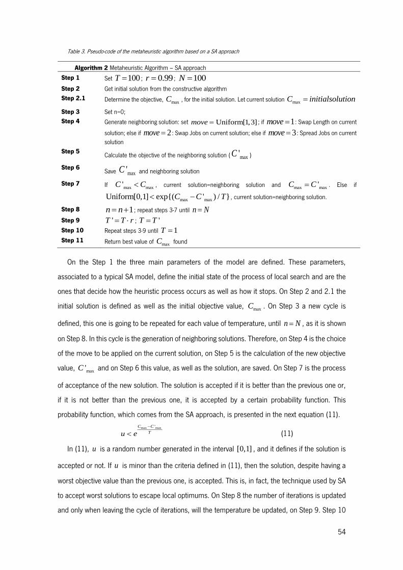
54

Table 3. Pseudo-code of the metaheuristic algorithm based on a SA approach

Algorithm 2 Metaheuristic Algorithm – SA approach

Step 1 Set 100T = ; 0.99r = ; 100N =

Step 2 Get initial solution from the constructive algorithm

Step 2.1 Determine the objective, maxC , for the initial solution. Let current solution maxC initialsolution=

Step 3 Set n=0;

Step 4 Generate neighboring solution: set Uniform[1,3]move = ; if 1move = : Swap Length on current

solution; else if 2move = : Swap Jobs on current solution; else if 3move = : Spread Jobs on current

solution

Step 5 Calculate the objective of the neighboring solution ( max'C )

Step 6 Save max'C and neighboring solution

Step 7 If max max'C C , current solution=neighboring solution and max max'C C= . Else if

max maxUniform[0,1] exp{( ' ) / }C C T − , current solution=neighboring solution.

Step 8 1n n= + ; repeat steps 3-7 until n N=

Step 9 'T T r= ; 'T T=

Step 10 Repeat steps 3-9 until 1T =

Step 11 Return best value of maxC found

On the Step 1 the three main parameters of the model are defined. These parameters,

associated to a typical SA model, define the initial state of the process of local search and are the

ones that decide how the heuristic process occurs as well as how it stops. On Step 2 and 2.1 the

initial solution is defined as well as the initial objective value, maxC . On Step 3 a new cycle is

defined, this one is going to be repeated for each value of temperature, until n N= , as it is shown

on Step 8. In this cycle is the generation of neighboring solutions. Therefore, on Step 4 is the choice

of the move to be applied on the current solution, on Step 5 is the calculation of the new objective

value, max'C and on Step 6 this value, as well as the solution, are saved. On Step 7 is the process

of acceptance of the new solution. The solution is accepted if it is better than the previous one or,

if it is not better than the previous one, it is accepted by a certain probability function. This

probability function, which comes from the SA approach, is presented in the next equation (11).

max max'C C

Tu e−

(11)

In (11), u is a random number generated in the interval [0,1] , and it defines if the solution is

accepted or not. If u is minor than the criteria defined in (11), then the solution, despite having a

worst objective value than the previous one, is accepted. This is, in fact, the technique used by SA

to accept worst solutions to escape local optimums. On Step 8 the number of iterations is updated

and only when leaving the cycle of iterations, will the temperature be updated, on Step 9. Step 10

55

defines the stop criterion, which is when the temperature is set to 1. Finally, on Step 11, the best

solution found on the local search is returned. This is an additional step, considering the typical SA

algorithm, and it is important because it returns the best solution found in all of the search process.

Without this step, what would happen is that, as the SA allows worst solutions under a certain

probability, the last solution found by this approach, could not be the best found in all process.

That is why on Step 6 all solutions are saved and on Step 11 only the best solution found is

presented, instead of the last one found.

Giving these three developed methods for solving the problem, in the next section it will be

shown how they were tested and implemented. It will be followed by a results analysis as well as

a discussion. The goal of this work is to solve the problem and present feasible, and when possible,

optimal solutions.

57

5. Computational Experiments

In this chapter the three different methods presented previously, the MILP model, the CA and

the SA algorithms are going to be tested. It is usual, and valuable, to include computational tests

of the proposed algorithms, and these tests aim to, for example, demonstrate the potential of new

algorithms in specific situations, demonstrate that an algorithm is practical, identify conditions

under which an algorithm performs best or worst, and compare competing algorithms (Hall &

Posner, 2001).

To perform the tests, it was necessary to generate data that could allow a good evaluation and

comparison of the three methods. Besides generating the data, to perform the tests, it was

necessary to implement the procedures. The MILP model was implemented using the AMPL

language and submitted in the NEOS Server and solved through the Gurobi solver. The heuristic

models were implemented in Java language and run on a PC with the following characteristics:

Intel Core i3-2365M with 1.40GHz and 4GB of RAM, in the operating system Windows 10. The

data description and respective computational results are presented in the next sections.

5.1. Instance Sets

Due to the lack of benchmark instances in the literature, the performance of the exact and

heuristic methods is going to be evaluated by solving randomly generated instances. These

instances are going to be generated based on previous work present in literature to have a variety

set of instances with different conditions and workloads. Some characteristics of the instances

generated, that are considered to be important for the computational evaluation (Hall & Posner,

2001), are, for example, the variety, the practical relevance, and the regularity. On one hand, the

variety is obtained through generating different sizes of instances. On the other hand, the practical

relevance and the regularity ensure that the data generated is similar to real-world scenarios and

that each instance is treated in a similar way, respectively.

The number of cement companies in study – each company defines a set of instances –, is

three. These three companies differ on the machine environment, or in other words, in the length

of the warehouse. In the Table 4 it is possible to see the main parameters of each company.

58

Table 4. Companies' characteristics

Company No. of Docking Bays No. of Forklifts No. of products Available

1 6 2 3

2 12 3 3

3 16 3 4

For more details on the loading rates for each product, at each docking bay, of the companies’

warehouses, check Appendix I. For each company, or set, several instances were generated varying

the job’s parameters. The job’s parameters include the number of jobs n , the type of product

requested for each job jt , the quantity of material requested jq and the releases dates of each

job jr . They were randomly generated and can cover different circumstances.

The number of jobs per set that will be considered are 10, 20, 50, 100, 200n = . These

values assure that the experiment will be done starting with small size problems to reasonable

large size ones. Each job parameter followed a different distribution, the type of product, jt , uses

a discrete distribution, presented in the Table 5 for each company. With this distribution it is

possible to distinguish the two most demanded products from the other(s). This way, the practical

relevance is ensured, since in every warehouse of every cement company in study, there are

products more requested than others.

Table 5. Discrete distribution of the demand for each type of product

jt % of the demand

Company 1 1 37,5% 2 37,5% 3 25,0%

Company 2 1 37,5% 2 37,5% 3 25,0%

Company 3 1 30,0% 2 30,0% 3 25,0% 4 15,0%

The quantity of material requested, jq uses a normal distribution: ~ ( 6, 2)jq N = = . For

the release dates, on the other hand, jr uses a uniform distribution: max~ [0, ]jr U R . Where, the

maxR measures the expected total processing time. It is calculated as the following equation (12)

suggests. avgq is the average amount of product requested, avgv is the average loading rate

considering all the docking bays and respective loading rates for each type of product, n is the

59

total number of jobs and avgm is the average length of batches given as the average between the

number of docking bays and the number of forklifts.

avg

avg avg

q n

v m (12)

Finally, the element on the uniform distribution of jr is given as {0.5,0.75,1,1.25,1.5}

and it is based on the work of authors such as (Chu, 1992; Kooli & Serairi, 2014; Selim Akturk &

Ozdemir, 2000), and it guarantees the spread of the release dates of the jobs. As the size of

gets larger, the release dates are more spread out. The goal is to analyze how the algorithms

behave in all kind of circumstances, including the times when the clients arrive to the facilities

closer or more distant from each other. The Table 6 gives a summary of all the parameters of the

problem already described as well as the number of alternatives of each parameter for each

instance, and the total number of instances generated.

Table 6. The parameters of the problem

Parameter Alternatives Values

n 5 10, 20, 50, 100, 200

jt 1 Presented in Table 5

jq 1 ~ (6,2)N

jr 5 max~ [0, ]U R , {0.5,0.75,1,1.25,1.5}

No. of Companies 3

Total no. of instances 75

5.2. Results and Discussion

Each one of the 75 instances generated in the last section was submitted to each one of the

algorithms: the MILP, CA and SA. For the SA algorithm, each instance was run six times, since the

SA algorithm is made by some probabilistic functions. The probability functions give the algorithm

some uncertainty and that is why it is usual to run it more than one time to see what range of

solutions it is capable to obtain. In this section all results will be presented as well as a discussion

of what they represent. In the Appendix II. the results are presented in tables with the computational

results for each value of n .

To start the analysis of the results, the following Gantt diagrams pretend to give a visual example

of how the solutions change according to the algorithm used. The example presented refers to the

60

Company 1, for 10n = and 1,5 = which is a solution where the CA could not reach the MILP

solution, but the SA did. In the Figure 6, Figure 7 and Figure 8 three different solutions are

presented, the Figure 6 is the one obtained through the CA, the Figure 7 is the worst solution

obtained with the SA algorithm and, finally, the Figure 8 is the one obtained with the MILP that is

equivalent to the best solution found by the SA.

Figure 6. Gantt diagram solution for the instance: Company 1, n=10 and 1.5 = using the CA.

Figure 7. Gantt diagram solution for the instance: Company 1, n=10 and 1.5 = using the SA.

Figure 8. Gantt diagram solution for the instance: Company 1, n=10 and 1.5 = using the MILP.

As it is possible to see from Figures 6, 7 and 8, as the solution evolves from CA to MILP model,

the objective function improves – the makespan goes from 46 minutes to 44,5 minutes – and

achieves a point where the work is concentrated in one region only. This is favorable mainly for the

warehouse’s resources since it appears to improve the workflow. In fact, with the schedule obtained

using the MILP model – the optimum solution – the forklifts can do the work all at once, since the

batches enter the warehouse almost one after another. The schedule of the SA algorithm solution

is better than the schedule of the CA, even it being the worst solution found by SA. The best solution

found by the SA algorithm is equal to the optimum solution provided by the MILP model and

presented in Figure 8. As it is possible to see the SA method has the capacity to improve the CA

solution and, in this case as it happened in other instances, the SA algorithm could really achieve

61

the optimum solution. The graphics of the Figures 9 to 13 include the deviation from the MILP

model solutions for the CA and SA models. Through the Figure 9 to Figure 13 it is also possible to

see in how many instances the SA algorithm could improve the CA solutions. For the case of the

SA solutions, it is the deviation between the best solution reached by the SA algorithm and the

solution achieved by the MILP model.

Figure 9. Deviation from the optimal for n=10 for each instance, starting with the Company 1 to Company 3, with increasing values of , for each company.

Figure 9 presents the results for 10n = . As it is possible to see, for the instances where the

CA did not reach the optimum value, 0dev , the SA algorithm, in all situations, could achieve, at

least one time, the solution reached by the MILP model, which for these instances is the optimum.


On the graph of Figure 10, that presents the results for 20n = , the SA method could not reach

the optimum value in all instances. There were five instances where the SA method did not achieve

the optimum value. However, the SA model could reach, at least one time in almost every instance,

solutions closer to the optimum value comparing with the solutions of the CA solutions. In other

words, the SA algorithm, in the instances where it failed to reach the optimum values, at least it

could improve the solutions first obtained with the CA. The only instance where this did not happen

was in the last instance which corresponds to the instance of the Company 3 and 1,5 = .


62

In the Figure 11, that presents the results for 50n = , there are instances where both CA and

SA reached the optimum values, there are other instances where the CA did not reach the optimum

but the SA did, there are other instances where neither the CA or SA reached the optimum but the

SA managed to improve the CA results and, finally there are instances where neither the CA or the

SA reached the optimum and the SA also did not manage to improve the CA solution. For these

three first graphics, besides the situations of improving or not improving CA solutions, or reaching

or not reaching the optimum, the values of the deviation are all 0 but still close to zero. This

proves that the solutions, even if they are not the optimum solutions, they are near to the optimum

which is a good signal about the efficiency of the algorithms.



For the two last graphs of Figures 12 and 13, there are instances where the deviation from the

MILP solution becomes 0 . Since the maximum computational time dispensed by the NEOS

server is 8 hours and, if by that time the MILP model did not has the time to test all possibilities,

what happens is that it returns a solution with no guarantees of optimality. In this sense, for some

larger instances the MILP model could not get to the optimum solution, or at least there are no

guarantees that the solution achieved is optimum, since it ran out of time. From the results,

presented in the Appendix II., it is possible to verify that this type of situation happened for 50n =

to the company 3 when 1,5 = ; for 100n = to the company 1 when 1,25 = and 1,5 = , to

company 2 when 1,5 = and to company 3 when 1,25 = and 1,5 = ; and for 200n = to

the company 1 when 1 = , 1,25 = and 1,5 = , to company 2 when 1 = , 1,25 = and

1,5 = , and finally, to company 3 when 1,25 = and 1,5 = . From here it is possible to see

63

that for larger instances, 50n and larger values of , the MILP model starts having

computational difficulties in finding the optimum solution, which is a signal of the problem difficulty.

For the case where the number of jobs increases, i.e., when the length of the instances gets bigger,

it was already expected that the problem started having computational difficulties. In fact, as the

instances get bigger, there are more combinations for the solver to compute and, at some point, it

cannot compute all the possibilities in a reasonable amount of time and the problem becomes

computationally difficult. This also gives some hints of the problem NP-hardness. On the other

hand, for the values, it was also expected for the instances to became hard to solve as the

values of grow since the problem is relatively simple when is small, because the release

dates are not scattered (Selim Akturk & Ozdemir, 2000). In fact, when is small, the problem

rapidly becomes a problem without release dates after having scheduled a few jobs, which is an

easier class of problems (Chu, 1992). Having these computational difficulties in consideration, it

is now possible to understand why there are cases where the deviation assumes a negative value

( 0 ). These cases, that start to happen for instances where 100n = and 200n = , as it is

possible to see on Figure 12 and Figure 13, occurred in instances where the MILP model could

not get to the optimum value and, both the CA and SA models achieved better values of makespan

than the MILP. This also proves the efficiency of the heuristic algorithms that, in shorter periods of

time, can achieve best solutions, for larger instances. In the Figure 14 and Figure 15 it is possible

to see how shorter, in average, these periods of time really are. The Figure 14 present a bar chart

with the average computational time for each method, in each company. The Figure 15 presents

a bar chart with the average computational time for each method, for each value. Note that for

the CA, comparing with the two other methods, the computational time needed to solve the

problem is so smaller that it is not possible to see the bar that corresponds to this method.

64

Figure 14. Average computational time for each method, for each company.

Figure 15. Average computational time for each algorithm, for each value of .

From Figure 14 and Figure 15 it is possible to confirm that when both instances get bigger and

release dates get spreader, the computational effort of the problem gets harder for the MILP model.

For the heuristic models, no matter the size of the instance or the level of spread of the release

dates, the computational time needed to solve the problem is, in average, always shorter than the

exact method approach. Despite the average computational difficulties of the MILP model,

considering the heuristic methods, there are some instances that it could reach the optimum

solution in a reasonable amount of time. In the Figure 16, Figure 17 and Figure 18, the evolution

of the computational time for each model, both exact and heuristics, in each company, for each

instance size, is presented.

6353,326852,28

8386,8

0,11 0,14 0,14

37,74 36,9440,74

0,00

10,00

20,00

30,00

40,00

50,00

60,00

70,00

80,00

90,00

100,00

0,00

1 000,00

2 000,00

3 000,00

4 000,00

5 000,00

6 000,00

7 000,00

8 000,00

9 000,00

1 2 3

Co

mp

uta

tio

nal

Tim

e (s

ec)

Companies

MILP

CA

SA

2624,931481,47

6235,07

10257,40

15388,47

0,13 0,13 0,13 0,12 0,14

35,90 39,23

40,2038,50 38,53

0,00

20,00

40,00

60,00

80,00

100,00

120,00

0

2000

4000

6000

8000

10000

12000

14000

16000

18000

0,5 0,75 1 1,25 1,5

Co

mp

uta

tio

nal

Tim

e (s

ec)

values

MILP

CA

SA

65

Figure 16. Evolution of the computational times per company for each n, for the MILP model.

Figure 17. Evolution of the computational times per company for each n, for the CA.

Figure 18. Evolution of the computational times per company for each n, for the SA algorithm.

5,2 9,4 11,6

84,614,2 32

557

5814,8 6478,2

11718,2

7207,6

12861,8

19401,621215,4

22550,4

0

5000

10000

15000

20000

25000

1 2 3

Co

mp

uta

tio

nal

Tim

e (s

ec)

Company

10

20

50

100

200

0,05 0,07

0,030,040,06 0,06

0,09 0,100,09

0,180,15

0,17

0,20

0,320,33

0,00

0,05

0,10

0,15

0,20

0,25

0,30

0,35

1 2 3

Co

mp

uta

tio

nal

Tim

e (s

ec)

Company

10

20

50

100

200

4,39 4,66 4,856,20 8,46 13,00

19,53 18,4034,06

49,59 49,2238,41

109,00103,96

113,38

0,00

20,00

40,00

60,00

80,00

100,00

120,00

1 2 3

Co

mp

uta

tio

nal

Tim

e (s

ec)

Companies

10

20

50

100

200

66

For the three methods implemented, when the number of jobs increases, so does the

computational time, as expected. For the MILP approach, it is clear why the computational time

increases, since this problem is characterized by being a combinatorial problem, and it was

something predictable already in the previous chapter of this work. For the heuristic models, the

computational time also increases since the steps that each one of the algorithms must follow, as

the number of jobs increases will take longer to compute. However, while the maximum average

computational time reached for the MILP model was almost 8 hours – without guarantees of

optimality –, for the CA it was 0,33 seconds and for the SA approach it was 114 seconds. With

these results of the differences of computational times for each algorithm and having in

consideration the previous study about the average deviation from the optimum for the heuristic

models, it is safe to say that solutions found by the heuristic models are of good quality and they

can give solutions near the optimum or even the optimum. To conclude, a final analysis was made

about the influence of the warehouses’ features in the achievement of good solutions comparatively

to the optimum. In the Figure 19 it is presented the percentages of cases where solutions provided

by the heuristic models were the same, best or worse than the ones provided by the MILP model.

Again, the solutions reach by the heuristic models are only better than the MILP when this last one

did not reach the optimality due to having reached the maximum computational time available by

NEOS server.

Figure 19. Percentage of solutions reached by the heuristic algorithms that are the same, best or worse than the ones provided by the MILP model.

For each company, 12% of the solutions found by the heuristic methods are better than the

ones reached by the MILP model. A possible explanation for this same percentage for each

company might be the fact that for each company, the MILP model had difficulties in the same

values of n , in this case, for the largest values of n . Plus, it is possible to verify a large difference

between the percentage of worst cases between the company 2 and the two others. This suggests

38,0%

68,0%

28,0%

12,0% 12,0% 12,0%

50,0%

20,0%

60,0%

0,0%

10,0%

20,0%

30,0%

40,0%

50,0%

60,0%

70,0%

80,0%

1 2 3

% o

f so

luti

on

s

Company

same

best

worst

67

that there is something in the company 2 that eases the process of achieving the optimum

solutions, since the percentage of better solution is the same for the three companies. From

company 1 to 2, what changes is the amount of docking bays available and the number of forklifts,

which consequently increases the number of alternatives where jobs could be assigned and the

number of resources to do the work. On the other hand, from company 2 to 3, what changes is

also the number of docking bays and the number of materials available. Looking to the Figure 19

it seems possible to assume that the company 2 has the most favorable conditions to allow the

algorithms to reach best values of the objective function, comparatively to the two other companies.

69

6. Conclusion

This dissertation presented a case study in the cement industry. Inserted in a project called

UH4SP, the goal of this dissertation was to study the operation of loading trucks in a warehouse,

related with the cement industry. Despite the link with the cement industry, this work aims to be a

contribution to other industries, since the operation of loading trucks in warehouses is a common

logistic process in several industries.

The literature review provided in this work proved the importance of the logistics and SCM in

the achievement of improvements for companies. These improvements usually come as

competitive advantages that companies can reach through the monitorization and the optimization

of their supply chains. Among the supply chain’s activities is the distribution. The distribution, as

the operation of delivering the final product or service to the final client, is given as an important

and critical activity. On one hand, the importance is given by the fact that the distribution has the

task to control whether the product or service reaches the final client in the right conditions and at

the right time. On the other hand, the critical characteristic is given by the fact that, if any mistake

or delay happens in the process of distribution, it can directly affect the final client, lowering the

service levels as well as the company reputation. The distribution itself is an activity that includes

other minor activities. Among others there is the warehousing activity. The warehousing is given as

an important activity to quickly answer variations in demand. To satisfy the clients’ orders in the

fastest time possible, having finished products available in stock becomes an imperative feature.

The warehousing activity must be efficient otherwise there will be unnecessary costs in stake. For

instances, if the stock level becomes higher than what is necessary, the company will incur in

avoidable costs. In order to achieve higher efficiency levels, decision-making activities related with

both the design and operations in the warehouse, must be optimized. Inside the warehouse

operations there is the shipping activity characterized by being the operation responsible for making

the product leave the warehouse. The shipping activity is in return characterized by decision-making

processes such as the scheduling and assignment of trucks – that usually are the means of

transport of the products – to docking bays. With the literature review made about all these topics

addressed so far – the distribution, the warehousing and the shipping – it was possible to give a

general framework of the real problem inside of what it is the scope of the logistics and SCM. In

70

addition, the topics of scheduling and the methodologies to solve scheduling problems were also

addressed in the literature review. The research about these topics provided a powerful tool to both

characterize and solve the real problem in study. One advantage of studying the literature, is that

it is possible to compare the already studied problems with problems that are still about to solve,

and with that comparison make conclusions about how to formalize and solve problems. Basically,

this was the main goal of studying the scheduling field. Only after understanding how scheduling

problems are defined and characterized, it was possible to characterize the real problem of this

dissertation. Plus, only with the right knowledge of how scheduling problems are solved, it was

possible to design the needed models to solve the real problem. Concluding, the literature review

made in this dissertation proved to be a great source of knowledge needed to frame, characterize,

formalize and solve the real problem.

Considering the knowledge acquired with the literature review, it was possible to study the real

problem as an analogy to the machine scheduling problem. But, after solving the problem, a

detailed characterization of it was necessary. First, and to better understand what type of industry

the cement industry is, a brief research about the state of this industry was addressed. With this

research it was possible to conclude that the cement industry is a growing industry and its growth

is directly linked to the globalization and the population growth. Being a growing industry involves

higher levels of efficiency to better meet the demand requirements. In what concerns the state of

the art of the shipping activity in the cement industry, it was not possible to find many studies about

the matter. This fact makes possible to conclude that this work addresses some contributions to

the shipping process in the cement industry, more precisely, to the process of scheduling and

assigning trucks to the warehouse’s docking bays. Plus, since no background was found and to

help the process of formalizing the problem, some assumptions were needed to simplify the

problem. The simplification of the problem is needed to later formalize it. After the formalization,

the problem was treated as a serial batch processing machine scheduling problem. To solve the

problem, an exact method, more specifically a MILP model, was developed. However, since this

method showed computational difficulties for larger instances and to overcome these difficulties,

two heuristics were further developed. The first one was created aiming to achieve a first feasible

solution. The second one was developed aiming to improve the solution obtained with the first

heuristic algorithm. Hence, the first heuristic is given as a Constructive Algorithm (CA), and the

second one as a metaheuristic method. The results obtained through computational tests showed

that for the instances where the MILP model was able to reach the optimum, both heuristics

71

presented solutions of good quality, some of them even reach the optimum. Plus, the average

computational time is larger for the MILP model (in the range of 1000 seconds), following the

metaheuristic (in the range of 114 seconds) and last the fast algorithm the CA (in the range of 0,3

seconds). For the cases where the MILP model could not reach the optimum solutions, due to

maximum computational time limits to process – being the limit 8 hours –, the heuristic algorithms

managed to achieve better solutions in less than one second for the CA, and less than one minute

for the metaheuristic method.

Regarding the future work proposals, first, a possible suggestion could be to try to create other

constructive algorithms, as well as other metaheuristics approaches, to compare with the ones

already developed in this work. With other methods it would be possible to understand the

limitations and/or advantages of the algorithms presented in this dissertation. Another idea would

be to test other moves in the metaheuristic. As the moves applied in metaheuristic approaches

are, usually, directly related to the solutions’ quality, to test other moves rather than the ones

implemented could provide another vision and would help to understand which moves are better.

Another challenge would be to transform the main problem in a shop scheduling problem since,

in some industries, it is possible for clients to require more than one type of product. If the clients

demand is more than one type of product, in analogy to the machine scheduling, is the same as

having a job with more than one operation. In other words, it is the same as having more than one

stage in the process. The problem in study in this dissertation would then be turned into a shop

scheduling problem and it could give origin to an all-new study.

To conclude, even if this work remains as a study framework for future implementations in the

real life, it showed up to be an innovative work and of high scientific value. Since, according to the

current literature studied, the number of studies regarding the scheduling of trucks to warehouses,

not including cross-docking warehouses, is a small number, this work proved to be a contribution

for future researches in the field. Therefore, to finish this dissertation and as an inspiring thought

for future researches that are trying to solve, or at least proposing ways to solve, problems, just

remember that, as Gaston Bachelard said, and citing: “The characteristic of scientific progress is

our knowing that we did not know”, because only knowing that we do not know, we will be able to

discover and learn. There is no learning without the unknowing.

73

References

Agudelo, I. (2009). Supply chain management in the cement industry. Massachusetts Institute of

Technology.

Aickelin, U., & Clark, A. (2011). Heuristics optimization. Journal of Operational Research Society,

62, 251–252.

Aitken, J. (1998). Supply Chain Integration within the Context of a Supplier Association. Cranfield

University.

Albers, S., & Brucker, P. (1993). The complexity of one-machine batching problems. Discrete

Applied Mathematics, 47(2), 87–107.

Allahverdi, A., Ng, C. T., Cheng, T. C. E., & Kovalyov, M. Y. (2008). A survey of scheduling problems

with setup times or costs. European Journal of Operational Research, 187(3), 985–1032.

AMPL Optimization Inc. (2018). AMPL. Retrieved July 11, 2018, from

https://ampl.com/products/solvers/

Amrina, E., & Vilsi, A. L. (2015). Key performance indicators for sustainable manufacturing

evaluation in cement industry. Procedia CIRP, 26, 19–23.

Amstel, R. P. van, & D’hert, G. (1996). Performance Indicators in Distribution. The International

Journal of Logistics Management, 7(1), 73–82.

Azizoglu, M., & Webster, S. (2001). Scheduling a batch processing machine with incompatible job

families. Computers and Industrial Engineering, 39(3–4), 325–335.

Baptiste, P. (2000). Batching identical jobs. Mathematical Methods of Operations Research, 52(3),

355–367.

Baptiste, P., & Jouglet, A. (2001). On Minimizing total tardiness in a serial batching problem. RAIRO

Operations Research, 35(1), 107–115.

Barreto, L., Amaral, A., & Pereira, T. (2017). Industry 4.0 implications in logistics: an overview.

Procedia Manufacturing, 13, 1245–1252.

Bazaraa, M. S., Jarvis, J. J., & Sherali, H. D. (2010). Linear Programming and Network Flows (4th

ed.). Hoboken, New Jersey: John Wiley & Sons, Inc.

Berg, J. P. V. Den, & Zijm, W. H. M. (1999). Models for warehouse management: Classification

and examples. International Journal of Production Economics, 59(1), 519–528.

74

Berghman, L., & Leus, R. (2015). Practical solutions for a dock assignment problem with trailer

transportation. European Journal of Operational Research, 246(3), 787–799.

Blum, C., & Roli, A. (2003). Metaheuristics in Combinatorial Optimization : Overview and

Conceptual Comparison. ACM Computing Surveys, 35(3), 268–308.

Brandimarte, P., & Zotteri, G. (2007). Introduction to Distribution Logistics (1st ed.). John Wiley &

Sons, Inc.

Brucker, P. (2004a). Classification of scheduling problems. In Scheduling Algorithms.

Brucker, P. (2004b). Computational Complexity. In Scheduling Algorithms (4th ed., pp. 37–56).

Berlin, Heidelberg, New York: Springer.

Brucker, P., Gladky, A., Hoogeveen, H., Kovalyov, M. Y., Potts, C. N., Tautenhahn, T., & Van De

Velde, S. L. (1998). Scheduling a batching machine. Journal of Scheduling, 1(1), 31–54.

https://doi.org/10.1002/(SICI)1099-1425(199806)1:1<31::AID-JOS4>3.0.CO;2-R

Brucker, P., Hurink, J., & Werner, F. (1997). Improving local search heuristics for some scheduling

problems. Part II. Discrete Applied Mathematics, 72(1–2), 47–69.

Brucker, P., & Knust, S. (2012a). Algorithms and Complexity. In Complex Scheduling (pp. 23–91).

GOR Publications.

Brucker, P., & Knust, S. (2012b). Scheduling Models. In GOR Publications (Ed.), Complex

Scheduling (pp. 1–28). Berlin, Heidelberg: Springer.

Chen, B., Potts, C. N., & Woeginger, G. J. (1998). A Review of Machine Scheduling: Complexity,

Algorithms and Approximability. In D.-Z. Du & P. M. Pardalos (Eds.), Handbook of

Combinatorial Optimization (Vol. 3, pp. 21–169). Kluwer Academic Publishers.

Christopher, M. (2011). Logistics & supply chain management (4th ed.).

Christopher, M. (2016). Logistics & supply chain management (5th ed.).

Chu, C. (1992). A Branch-And-Bound Algorithm to Minimize Total Tardiness with Different Release

Dates. Naval Research Logistics, 39, 265–283.

Damand, D., Barth, M., & Lepori, E. (2017). Problem Graph for Warehousing Design. In Cavallucci

D. (Ed.), TRIZ – The Theory of Inventive Problem Solving (pp. 105–128). Springer, Cham.

Damodaran, P., Ghrayeb, O., & Guttikonda, M. C. (2013). GRASP to minimize makespan for a

capacitated batch-processing machine. International Journal of Advanced Manufacturing

Technology, 68(1–4), 407–414. https://doi.org/10.1007/s00170-013-4737-z

Dorigo, M., & Stützle, T. (2003). The ant colony optimization metaheuristic: algorithms,

applications and advances. In G. F. & K. G.A. (Eds.), Handbook of Metaheuristics (Vol. 57).

75

Boston, MA: Springer.

Dowsland, K. A., & Thompson, J. M. (2012). Simulated Annealing. In G. Rozenberg, T. Bäck, & J.

N. Kok (Eds.), Handbook of Natural Computing (pp. 1623–1655). Springer, Berlin,

Heidelberg.

Du, J., & Leung, J. Y.-T. (1990). Mathematics of Operations Research Minimizing Total Tardiness

on One Machine is NP-Hard. Mathematics of Operations Research, 15(3), 483–495.

Dürr, C., Knust, S., Prot, D., & Vásquez, Ó. C. (2016). The Scheduling Zoo.

Elhasia, T., Noche, B., & Zhao, L. (2013). Simulation of a Sustainable Cement Supply Chain ;

Proposal Model Review. Engineering and Technology, 7(3), 464–472.

Fawcett, S. E., Birou, L., & Cofield Taylor, B. (1993). Supporting Global Operations through

Logistics and Purchasing. International Journal of Physical Distribution & Logistics

Management, 23(4), 3–11.

Fonseca, J., Alves, R., Macedo, A. R., Carvalho, M. S., Pereira, G., & Oliveira, J. A. (2018). Integer

Programming Model for Ship Loading Management. In J. Machado, F. Soares, & G. Veiga

(Eds.), Innovation, Engineering and Entrepreneurship. HELIX 2018. Lecture Notes in

Electrical Engineering (Vol. 505). Springer, Cham.

Ford, M. (2015). Industry 4.0: Who Benefits? SMT: Surface Mount Technology, 30(7), 52–55.

Fourer, R., Gay, D. M., & Kernighan, B. W. (1990). AMPL : A Mathematical Programming Language.

Management Science, 36, 519–554.

Gandomi, A. H., Yang, X., Talatahari, S., & Alavi, A. H. (2013). Metaheuristic Algorithms in Modeling

and Optimization. In Metaheuristic Applications in Structures and Infrastructures (1st ed., pp.

1–24). Elsevier Inc.

Gendreau, M., & Potvin, J.-Y. (2005). Metaheuristics in Combinatorial Optimization. Annals of

Operations Research, 140, 189–213.

Glover, F. (1986). Future paths for integer programming and links to artificial intelligence.

Computers & Operations Research, 13(5), 533–549.

Goldreich, O. (2008). Computational Complexity : A Conceptual Perspective. ACM SIGACT, 39(3),

35–39.

Graham, R. L., Lawler, E. L., Lenstra, J. K., & Kan, A. H. G. R. (1979). Optimization and

approximation in deterministic sequencing and scheduling: a survey. Annals of Operations

Research, 5, 287–326.

Groner, R., & Groner, M. (1983). Methods of Heuristics. In R. Groner, M. Groner, & W. F. Bischof

76

(Eds.), Proceedings of an interdisciplinary symposium (pp. 1–18). Bern, Switzerland:

Lawrence Erlabaum Associates, Inc.

Gu, J., Goetschalckx, M., & McGinnis, L. F. (2007). Research on warehouse operation: A

comprehensive review. European Journal of Operational Research, 177(1), 1–21.

Gundlach, G. T., Bolumole, Y. A., Eltantawy, R. A., & Frankel, R. (2006). The changing landscape

of supply chain management , marketing channels of distribution , logistics and purchasing.

Journal of Business & Industrial Marketing, 21(7), 428–438.

Hall, N. G., & Posner, M. E. (2001). Generating Experimental Data for Computational Testing with

Machine Scheduling Applications. Operations Research, 49(6), 854–865.

Hofmann, E., & Rüsch, M. (2017). Industry 4.0 and the current status as well as future prospects

on logistics. Computers in Industry, 89, 23–34.

Huang, S. H., & Keskar, H. (2007). Comprehensive and configurable metrics for supplier selection.

Int. J. Production Economics, 105, 510–523.

Hugos, M. (2018). Essentials of Supply Chain Management (4th ed.). New Jersey: John Wiley &

Sons, Inc.

Kadhim, A. M., Ali, S. K., & Kassim, M. M. (2018). Solving Machine Scheduling Problem under

Fuzzy Processing Time using the Simulated Annealing Method. Journal of Progressive

Research in Mathematics, 14(1), 2308–2317.

Kadhim, A. M., & Hanoon, S. K. (2018). Local search Methods to Solve The Sum of Two Objective

Functions. Journal of Progressive Research in Mathematics, 13(3), 2245–2264.

Kooli, A., & Serairi, M. (2014). A mixed integer programming approach for the single machine

problem with unequal release dates. Computers and Operations Research, 51, 323–330.

Kozakowska, N., & Taljedal, H. (2017). A Qualitative Study of Operational Excellence at a Logistics

Service Provider. Chalmers University of Techonology.

Lenstra, J. K., Rinnooy Kan, A. H. G., & Brucker, P. (1977). Complexity of Machine Scheduling

Problems. Annals of Discrete Mathematics, 1(8), 343–362.

Lewis, C. (2008). Linear Programming : Theory and Applications.

Lummus, R. R., & Vokurka, R. J. (1999). Defining supply chain management : a historical

perspective and practical guidelines. Industrial Management & Data Systems, 99(1), 11–17.

Mangan, J., & Lalwani, C. (2016). Global Logistics and Supply Chain Management (3rd ed.).

Meindl, B., & Templ, M. (2013). Analysis of Commercial and Free and Open Source Solvers for the

Cell Suppression Problem. Transactions on Data Privacy, 6, 147–159.

77

Meiswinkel, S. (2018). Mechanism Design and Machine Scheduling : Literature Review. In

Combinatorial Optimization and Machanism Design Problems Arising at Container Ports (pp.

15–30). Springer Gabler, Wiesbaden.

Melouk, S., Damodaran, P., & Chang, P. Y. (2004). Minimizing makespan for single machine batch

processing with non-identical job sizes using simulated annealing. International Journal of

Production Economics, 87(2), 141–147.

Mentzer, J. T., Esper, T. L., Stank, T. P., & Esper, T. L. (2008). Supply chain management and its

relationship to logistics, marketing, production, and operations management. Journal of

Business Logistics, 29(1), 31–46.

Noche, B., & Elhasia, T. (2013). Approach to innovative supply chain strategies in cement industry ;

Analysis and Model simulation. In Procedia - Social and Behavioral Sciences. The Second

International Conference on Leadership, Technology and Innovation Management Approach

(Vol. 75, pp. 359–369). Elsevier Ltd.

Oliveira, J. A. (2007). Scheduling the truckload operations in automatic warehouses. European

Journal of Operational Research, 179(3), 723–735.

Osman, I. H., & Laporte, G. (1996). Metaheuristics: A bibliography. Annals of Operations Research,

63(5), 511–623.

Pinedo, M. L. (2016a). Complexity Theory. In Scheduling: Theory, Algorithms, and Systems (5th

ed., pp. 589–602). New York: Springer.

Pinedo, M. L. (2016b). Deterministic Models: Preliminaries. In Scheduling: Theory, Algorithms, and

Systems (5th ed., pp. 13–33). New York: Springer.

Pinedo, M. L. (2016c). Introduction. In Scheduling: Theory, Algorithms, and Systems (5th ed., pp.

1–10). New York: Springer.

Pinedo, M. L. (2016d). Scheduling: Theory, Algorithms, and Systems. Scheduling: Theory,

Algorithms, and Systems (5th ed.). New York: Springer.

Pochet, Y., & Wolsey, L. A. (2006). Mixed Integer Programming Algorithms. In Production Planning

by Mixed Integer Programming (1st ed., pp. 77–113). Springer-Verlag New York.

Potts, C. N., & Kovalyov, M. Y. (2000). Scheduling with batching: a review. European Journal of

Operational Research, 120(2), 228–249.

Rezaei, J., Hemmes, A., & Tavasszy, L. (2017). Multi-criteria decision-making for complex bundling

configurations in surface transportation of air freight. Journal of Air Transport Management,

61, 95–105.

78

Roblek, V., Meško, M., & Krapež, A. (2016). A Complex View of Industry 4.0. SAGE Open, 6(2), 1–

11.

Roser, M. (2018). Economic Growth. Retrieved July 25, 2018, from

https://ourworldindata.org/economic-growth

Roser, M., & Ortiz-Ospina, E. (2018). World Population Growth. Retrieved July 25, 2018, from

https://ourworldindata.org/world-population-growth

Rouwenhorst, B., Reuter, B., Stockrahm, V., Houtum, G. J. van, Mantel, R. J., & Zijm, W. H. M.

(2000). Warehouse design and control: Framework and literature review. European Journal

of Operational Research, 122, 515–533.

Rushton, A., Croucher, P., & Baker, P. (2010). Introduction to logistics and distribution. In The

Handbook of Logistics and Distribution Management: Understanding the Supply Chain (pp.

3–14).

Sampson, S. E., & Weiss, E. N. (1993). Local Search Techniques for the Generalized Resource

Constrained Project Scheduling Problem. Naval Research Logistics, 40, 665–675.

Sel, Ç., & Hamzadayi, A. (2018). A Simulated Annealing approach based simulation-optimisation

to the dynamic job-shop scheduling problem. Pamukkale University Journal of Engineering

Sciences, 24(4), 665–674.

Selim Akturk, M., & Ozdemir, D. (2000). An exact approach to minimizing total weighted tardiness

with release dates. IIE Transactions, 32(11), 1091–1101.

Selim, T. H., & Salem, A. S. (2010). Global Cement Industry: Competitive and Institutional

Frameworks. Journal of Strategic Management Education, 7.

Seth, N., Deshmukh, S. G., & Vrat, P. (2006). A framework for measurement of quality of service

in supply chains. Supply Chain Management: An International Journal, 11(1), 82–94.

Shen, W., Liu, Y., Yan, B., Wang, J., He, P., Zhou, C., … Xu, G. (2017). Cement industry of China:

Driving force, environment impact and sustainable development. Renewable and Sustainable

Energy Reviews, 75, 618–628.

Silver, E. A. (2002). An overview of heuristic solution methods.

Stadtler, H. (2015). Supply Chain Management: An Overview. In H. Stadtler, C. Kilger, & H. Meyr

(Eds.), Supply Chain Management and Advanced Planning (pp. 3–28). Springer, Berlin,

Heidelberg: Springer Texts in Business and Economics.

Taha, H. A. (2007). Operations Research: an introduction. (M. J. Horton, H. Stark, V. O’Brien, &

D. A. George, Eds.) (8th ed.). New Jersey: Pearson Education, Inc.

79

Tjahjono, B., Esplugues, C., Ares, E., & Pelaez, G. (2017). What does Industry 4.0 mean to Supply

Chain? Procedia Manufacturing, 13, 1175–1182.

USGS. (2018). Cement Statistics and Information.

Vanderbei, R. J. (2014). Linear Programming: Foundations and Extensions. International Series in

Operations Research and Management Science, 196.

Webster, S., & Baker, K. (1995). Scheduling Groups of Jobs on a Single Machine. Operations

Research, 43(4), 692–703.

Wisconsin Institutes for Discovery. (2018). NEOS Server. Retrieved July 11, 2018, from

https://neos-server.org/neos/

Yang, X.-S. (2011). Review of Metaheuristics and Generalized Evolutionary Walk Algorithm. Int. J.

Bio-Inspired Computation, 3(2), 77–84.

Yuan, J. J., Liu, Z. H., Ng, C. T., & Cheng, T. C. E. (2006). Single machine batch scheduling

problem with family setup times and release dates to minimize makespan. Journal of

Scheduling, 9(6), 499–513.

81

Appendix

Appendix I.

Table 7. Loading Rates for each product, at each docking bay, in pallets per minute, for Company 1

Product WAREHOUSE CONFIGURATION

1 1,0 1,0 0,8 0,5 0,2 0,2

2 0,2 0,2 0,5 0,8 1 1

3 0,2 0,2 0,5 1 0,5 0,2

DB1 DB2 DB3 DB4 DB5 DB6

Table 8. Loading rates for each product, at each docking bay, in pallets per minute, for Company 2


1 1,0 1,0 0,8 0,5 0,5 0,2 0,2 0,5 0,5 0,8 1 1

2 0,5 0,8 1 1 0,8 0,5 0,5 0,8 1 1 0,8 0,5

3 0,2 0,2 0,2 0,5 0,8 1 1 0,8 0,5 0,2 0,2 0,2

DB1 DB2 DB3 DB4 DB5 DB6 DB7 DB8 DB9 DB10 DB11 DB12

Table 9. Loading rates for each product, at each docking bay, in pallets per minute, for Company 3


1 1 1 0,8 0,8 0,5 0,5 0,2 0,2 0,1 0,1 0,1 0,1 0,1 0,1 0,1 0,1

2 0,5 0,5 0,8 0,8 1,0 1,0 0,8 0,8 0,5 0,5 0,2 0,2 0,1 0,1 0,1 0,1

3 0,1 0,1 0,1 0,1 0,2 0,2 0,5 0,5 0,8 0,8 1 1 0,8 0,8 0,5 0,5

4 0,1 0,1 0,1 0,1 0,1 0,1 0,1 0,1 0,2 0,2 0,5 0,5 0,8 0,8 1 1 DB1 DB2 DB3 DB4 DB5 DB6 DB7 DB8 DB9 DB10 DB11 DB12 BD13 DB14 DB15 DB16

82

Appendix II.

Table 10, Computational results for n=10

Company

MILP CA SA

maxC CT (sec) No.

Batch maxC CT (sec) No.

Batch Dev

Best

maxC Avg

maxC Worst

maxC

Avg CT

(sec)

Avg No. Batch

Dev

1

0,5 28,5 6,00 5 28,5 0,08 5 0,0E+00 28,5 28,5 28,5 4,40 5 0,0E+00

0,75 28,5 5,00 5 28,5 0,07 5 0,0E+00 28,5 28,5 28,5 4,32 5 0,0E+00

1 32,5 5,00 5 32,5 0,04 5 0,0E+00 32,5 32,5 32,5 4,12 5 0,0E+00

1,25 36,5 5,00 5 36,5 0,04 5 0,0E+00 36,5 36,5 36,5 4,91 5 0,0E+00

1,5 44,5 5,00 4 46 0,03 5 3,3E-02 44,5 44,8 45 4,20 4 7,4E-03

2

0,5 23 11,00 3 23,6 0,09 3 2,5E-02 23 23 23 4,85 3 0,0E+00

0,75 22 10,00 3 22 0,04 3 0,0E+00 22 22 22 4,71 3 0,0E+00

1 22 5,00 3 22 0,05 3 0,0E+00 22 22 22 4,40 3 0,0E+00

1,25 23 16,00 3 24 0,13 3 4,2E-02 23 23 23 4,73 3 0,0E+00

1,5 27,7 5,00 3 27,7 0,04 3 0,0E+00 27,7 27,7 27,7 4,61 3 0,0E+00

3

0,5 23,3 6,00 3 23,3 0,03 3 0,0E+00 23,3 23,3 23,3 4,54 3 0,0E+00

0,75 25,3 6,00 3 26,3 0,03 3 3,8E-02 25,3 25,3 25,3 4,92 3 0,0E+00

1 28,3 10,00 3 28,3 0,03 3 0,0E+00 28,3 28,3 28,3 5,04 3 0,0E+00

1,25 31 26,00 3 31,7 0,05 3 2,2E-02 31 31 31 5,06 3 0,0E+00

1,5 28,3 10,00 3 29,7 0,03 3 4,7E-02 28,3 28,3 28,3 4,67 3 0,0E+00

Table 11. Computational results for n=20

Company

MILP CA SA

maxC CT (sec) No.


Batch Dev

Best

maxC Avg

maxC Worst

maxC

Avg CT

(sec)

Avg No. Batch

Dev

1

0,5 63 5 9 66,5 0,03 10 5,3E-02 63 63,5 64,5 6,03 7,8 7,9E-03

0,75 63 6 9 64 0,05 10 1,6E-02 63 63,7 64 6,07 9,7 1,1E-02

1 68 10 9 75 0,05 10 9,3E-02 71 72,6 74 6,08 9 6,3E-02

1,25 84 281 9 86,5 0,03 10 2,9E-02 84,5 85,4 86,5 6,49 9 1,6E-02

1,5 94 121 7 98 0,05 10 4,1E-02 95 96,8 98 6,32 8,7 2,9E-02

2

0,5 40 10 6 40 0,04 6 0,0E+00 40 40 40 8,82 6 0,0E+00

0,75 39 5 6 39 0,12 6 0,0E+00 39 39 39 9,05 6 0,0E+00

1 40 15 6 40 0,05 6 0,0E+00 40 40 40 8,20 6 0,0E+00

1,25 42 15 6 42 0,04 6 0,0E+00 42 42 42 8,04 6 0,0E+00

1,5 45 26 6 45 0,05 6 0,0E+00 45 45 45 8,19 6 0,0E+00

3

0,5 42 25 5 43,6 0,07 6 3,7E-02 42 42,2 42,5 12,46 5 4,7E-03

0,75 41 25 6 41,4 0,05 6 9,7E-03 41 41,2 41,4 14,82 6 4,9E-03

1 41 5 6 42,2 0,06 6 2,8E-02 41,3 41,7 42,2 12,50 6 1,6E-02

1,25 48 10 6 48,8 0,09 6 1,6E-02 48 48,3 48,5 17,29 6 6,2E-03

1,5 54,7 95 6 55,7 0,04 6 1,8E-02 55,7 55,7 55,7 7,94 6 1,8E-02

83


Company

MILP CA SA

maxC CT (sec) No.


Batch Dev

Best

maxC Avg

maxC Worst

maxC

Avg CT

(sec)

Avg No. Batch

Dev

1

0,5 162,5 31 25 166,5 0,09 25 2,4E-02 162,5 163,3 164,5 19,25 22 4,9E-03

0,75 166,5 286 25 166,5 0,07 25 0,0E+00 166,5 166,5 166,5 22,12 23,7 0,0E+00

1 164,5 60 24 164,5 0,15 25 0,0E+00 164,5 164,5 164,5 18,68 24,7 0,0E+00

1,25 184 1587 20 188,5 0,09 25 2,4E-02 188,5 188,5 188,5 17,67 23,8 2,4E-02

1,5 220 821 21 220 0,07 25 0,0E+00 220 220,0 220 19,92 20,5 0,0E+00

2

0,5 98,3 45 14 98,3 0,05 16 0,0E+00 98,3 98,3 98,3 17,20 15,2 0,0E+00

0,75 99 75 15 99 0,16 16 0,0E+00 99 99 99 15,71 15,5 0,0E+00

1 98,3 70 16 98,4 0,09 16 1,0E-03 98,4 98,4 98,4 12,51 15,5 1,0E-03

1,25 100 160 15 100,6 0,07 16 6,0E-03 100 100,3 100,6 25,43 13,7 3,0E-03

1,5 110,3 28724 15 110,3 0,15 16 0,0E+00 110,3 110,3 110,3 21,16 15,7 0,0E+00

3

0,5 95 45 14 95,4 0,07 16 4,2E-03 95 95,3 95,4 26,03 15,3 3,1E-03

0,75 95 35 15 95,4 0,05 16 4,2E-03 95 95,3 95,4 23,40 15,5 3,1E-03

1 97 100 16 97,7 0,10 16 7,2E-03 97 97,3 97,7 34,00 16 3,1E-03

1,25 105,7 3504 15 108,8 0,08 16 2,8E-02 108,3 108,5 108,8 39,62 15,7 2,6E-02

1,5 112,7 28707 15 116,7 0,14 16 3,4E-02 116,7 116,7 116,7 47,23 15,5 3,4E-02


Company

MILP CA SA

maxC CT (sec) No.


Batch Dev

Best

maxC Avg

maxC Worst

maxC

Avg CT

(sec)

Avg No.

Batch Dev

1

0,5 293 26 49 302 0,20 50 3,0E-02 293 295,5 297,5 46,10 49 8,5E-03

0,75 297 141 49 311,5 0,12 50 4,7E-02 298 301,4 304 41,54 49 1,5E-02

1 296 1002 49 296 0,10 49 0,0E+00 296 296 296 54,73 49,2 0,0E+00

1,25 338 28714 29 341 0,17 50 8,8E-03 338 339,3 341 50,88 49 3,8E-03

1,5 398 28708 26 397 0,29 50 -2,5E-03 397 397,0 397 54,68 50 -2,5E-03

2

0,5 206 1712 32 206 0,10 33 0,0E+00 206 206 206 56,64 31,3 0,0E+00

0,75 207 641 33 207 0,16 33 0,0E+00 207 207 207 50,40 31,5 0,0E+00

1 206 321 32 206 0,10 33 0,0E+00 206 206 206 54,96 30,2 0,0E+00

1,25 209 4655 29 209 0,10 33 0,0E+00 209 209 209 47,62 31,3 0,0E+00

1,5 218 28709 21 213,7 0,30 33 -2,0E-02 213,7 213,7 213,7 36,48 31,8 -2,0E-02

3

0,5 197,3 245 31 198,3 0,22 33 5,0E-03 198 198,2 198,3 45,93 32,2 4,5E-03

0,75 198,3 376 32 198,9 0,13 33 3,0E-03 198,3 198,8 198,9 39,93 31,5 2,5E-03

1 200,3 6252 31 201,8 0,26 33 7,4E-03 201,2 201,5 201,8 37,50 31,75 6,0E-03

1,25 204,7 28717 30 204,7 0,11 33 0,0E+00 204,7 204,7 204,7 36,06 32,8 0,0E+00

1,5 225 28719 22 221,7 0,13 33 -1,5E-02 221,3 221,6 221,7 32,63 32,7 -1,5E-02

84


Company

MILP CA SA

maxC CT (sec) No.


Batch Dev

Best

maxC Avg

maxC Worst

maxC

Avg CT

(sec)

Avg No.

Batch Dev

1

0,5 617 2928 91 639,5 0,24 100 3,5E-02 623,5 624,9 625,5 96,70 96,8 1,3E-02

0,75 619 7918 90 639,5 0,16 100 3,2E-02 628,5 630,2 632 113,40 98 1,8E-02

1 643 28720 74 640,5 0,24 100 -3,9E-03 634 637,9 640,5 116,23 99,2 -8,0E-03

1,25 740,5 28723 55 736,5 0,18 100 -5,4E-03 735,5 736,3 736,5 105,98 98,2 -5,7E-03

1,5 859 28719 50 862,5 0,19 100 4,1E-03 860 861,2 862,5 112,67 98 2,6E-03

2

0,5 414,7 13658 58 415 0,36 66 7,2E-04 415 415 415 91,00 64,7 7,2E-04

0,75 415,7 6227 62 416,8 0,33 66 2,6E-03 416,1 416,3 416,6 86,54 59,7 1,4E-03

1 418,7 28729 62 419,2 0,29 66 1,2E-03 418,7 418,8 419,2 130,33 63,8 2,4E-04

1,25 436,7 28734 54 415,7 0,26 66 -5,1E-02 415,7 415,7 415,7 95,81 65,3 -5,1E-02

1,5 466 28729 50 433,7 0,36 66 -7,4E-02 427 431,1 433,7 116,10 64,7 -8,1E-02

3

0,5 413 20621 66 416,9 0,32 66 9,4E-03 414,5 415,6 416,5 98,56 63,5 6,3E-03

0,75 416 6466 65 417,1 0,38 66 2,6E-03 416,9 417,1 417,1 151,48 65,7 2,6E-03

1 411 28222 65 414,4 0,37 66 8,3E-03 413,7 413,9 414,4 103,76 65,3 7,0E-03

1,25 463,7 28714 50 426,3 0,36 66 -8,8E-02 424,6 425,9 426,3 111,95 65,2 -8,9E-02

1,5 510,3 28729 41 459 0,23 66 -1,1E-01 458,3 458,9 459 101,15 65,5 -1,1E-01

ana regina oliveira macedo - repositorium.sdum.uminho.pt

Documents