rock stresses - crc press online · 2020-03-23 · rock stresses 115 of that expansion is governed...

109

4Rock Stresses

No discussion of fracturing is possible without first discussing in situ stresses since these stresses dominate the fracturing process. As described in the following, the fracture will form perpendicular to the minimum in situ stress—thus the injection pressure must be greater than this minimum. In this way, in situ stresses control injection pressure and thus dominate well construction requirements and required hydraulic horsepower to pump the treatment. After the fracture forms and propped open, this minimum stress acts to crush the proppant, thus determining the type of proppant required. In situ stresses dominate the fracturing process.

This chapter discusses building a rock stress log, what assumptions are made, and how to minimize uncertainty. Pore pressure and calculations on how to determine effective in situ stress are included. How everything in fracturing flows from in situ stress, how/why this must be calibrated, and examples of stress test methods are included, not actually detailed discus-sions of such testing. This is discussed in Chapter 8.

Introduction

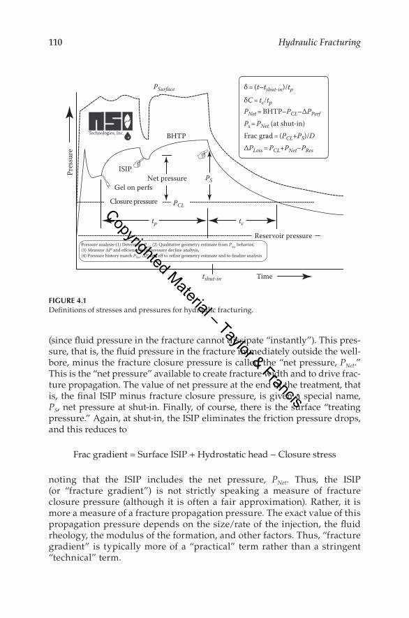
Prior to a discussion of in situ stress, some definitions may be in order. One thing hydraulic fracturing has in abundance is “pressures” (Figure 4.1). First, of course, is reservoir pressure. Above that is a value called “fracture closure pressure” or “closure stress.” This is equal to and the same as the minimum in situ stress. This is often (but not always) the same as the minimum hori-zontal stress (implying that most fractures are vertical since fractures always form perpendicular to the minimum in situ stress).

After pumping starts, the pressure inside the wellbore is the bottom-hole treating pressure (BHTP), and if the pumps are suddenly shut in, we see a sudden loss in bottom-hole pressure, and this sudden loss indicates that this loss was some form of downhole friction (pure orifice perforation fric-tion in the simplest case), followed by an instant shut-in pressure (ISIP). This ISIP equals the injection pressure in the fracture, right outside the wellbore

Copyrighted Material – Taylor & Francis

110 Hydraulic Fracturing

(since fluid pressure in the fracture cannot dissipate “instantly”). This pres-sure, that is, the fluid pressure in the fracture immediately outside the well-bore, minus the fracture closure pressure is called the “net pressure, PNet.” This is the “net pressure” available to create fracture width and to drive frac-ture propagation. The value of net pressure at the end of the treatment, that is, the final ISIP minus fracture closure pressure, is given a special name, PS, net pressure at shut-in. Finally, of course, there is the surface “treating pressure.” Again, at shut-in, the ISIP eliminates the friction pressure drops, and this reduces to

Frac gradient = Surface ISIP + Hydrostatic head − Closure stress

noting that the ISIP includes the net pressure, PNet. Thus, the ISIP (or “ fracture gradient”) is not strictly speaking a measure of fracture closure pressure (although it is often a fair approximation). Rather, it is more a measure of a fracture propagation pressure. The exact value of this propagation pressure depends on the size/rate of the injection, the fluid rheology, the modulus of the formation, and other factors. Thus, “fracture gradient” is typically more of a “practical” term rather than a stringent “technical” term.

PSurface δ = (t–tshut-in)/tp

δC = tc/tpPNet = BHTP–PCL–ΔPPerf

Ps = PNet (at shut-in)Frac grad = (PCL+PS)/DΔPLoss = PCL+PNet–PRes

BHTP

ISIP

Technologies, Inc.

Net pressureGel on perfs

Pres

sure

PCL

PS

tp tc

Timetshut-in

Closure pressure

Pressure analysis-(1) Determine PCL, (2) Qualitative geometry estimate from PNet behavior,(3) Measure ΔP' and effciency from pressure decline analysis,(4) Pressure history match PNet, ΔP' and eff to refine geometry estimate and to finalize analysis

Reservoir pressure

Figure 4.1Definitions of stresses and pressures for hydraulic fracturing.


111Rock Stresses

History

When fracturing was first introduced in 1949, it was assumed that all hydrau-lic fractures were horizontal based on early, shallow experiments. Indeed, the original Stanolind (later Amoco) patent specifically used the word “horizontal.” It quickly became evident this was incorrect (groundbreaking work by Hubbert and Willis, 1957), but despite much discussion and contro-versy, the patent was never tested. Legally, fractures remained horizontal for 17 years before suddenly becoming mostly vertical! Such is the vagaries of the legal system as compared to the physical world (Brown, 1978).

VerticalStress

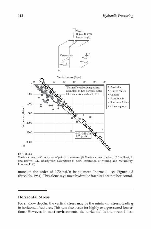
Proper hydraulic fracture treatment design requires knowledge of every piece of information in a well file, along with some information normally not found in any well file! This begins with in situ stress, geology, and geologic structure creating the stress. Stress, of course, is defined as “force/area” such as the weight of the overburden per square in. (or cm2). In fact, as pictured in Figure 4.2a, the vertical stress is in nearly all cases equal to the weight of the overburden per unit area. Figure 4.2b includes some measured val-ues of the vertical stress collected from mining and construction projects (Brown, 1978). The vertical stress/overburden is quite variable at shallow depths but “settles down” around 0.023 MPa/m (1.05 psi/ft). Direct density measurements generally show a lower value on the order of 1.0–1.05 psi/ft (0.0225 MPa/m) (equivalent to a 10%–12%, water-filled porosity sandstone from surface to total depth [TD]). Of course offshore, attention must be paid, and corrections made for water depth. In rare cases, upward, uplift forces (e.g., salt diapers) can create subsurface vertical stress locally greater than the weight of the overburden.

In the earth, each block of rock is acted on by three principle stresses (i.e., three stresses oriented such that they act purely to compress the rock, not shear/twist it). Given sufficient geologic time, stress always returns to the condition pictured in Figure 4.2a (i.e., one of the principal stresses is the vertical stress)—gravity is patient! Given this condition, a fracture must be either vertical or horizontal since the fracture will be perpendicular to the minimum of these three stresses. However, in active tectonic areas, it is pos-sible to have shorter term shear stresses acting on the rock mass such that “inclined fractures may be possible” (Wright, 1997).

Typical field data, on the other hand, nearly universally show fracture prop-agation pressures or “fracture gradients” much less than 1.0 psi/ft, something



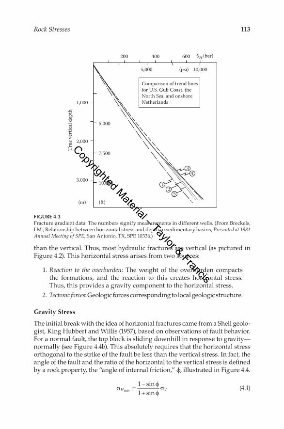
more on the order of 0.70 psi/ft being more “normal”—see Figure 4.3 (Breckels, 1981). This alone says most hydraulic fractures are not horizontal.

HorizontalStress

For shallow depths, the vertical stress may be the minimum stress, leading to horizontal fractures. This can also occur for highly overpressured forma-tions. However, in most environments, the horizontal in situ stress is less

00

500

1000

1500

2000

2500

3000

0.023 MPa/m1.05 psi/ft

Australia“Normal” overburden gradientequivalent to 12% porosity, water-filled rock from surface to TD

United StatesCanadaScandinaviaSouthern AfricaOther regions

Vert

ical

dep

th (m

)

10 20 30Vertical stress (Mpa)

40 50 60 70

(σHmax)(σHmin)

σmin

σmax(Equal to over-burden, σV?)

(a)

(b)

σintermediate

Figure 4.2Vertical stress. (a) Orientation of principal stresses. (b) Vertical stress gradient. (After Hoek, E. and Brown, E.T., Undergrown Excavations in Rock, Institution of Mining and Metallurgy, London, U.K.)


113Rock Stresses

than the vertical. Thus, most hydraulic fractures are vertical (as pictured in Figure 4.2). This horizontal stress arises from two sources:

1. Reaction to the overburden: The weight of the overburden compacts the formations, and the reaction to this creates horizontal stress. Thus, this provides a gravity component to the horizontal stress.

2. Tectonic forces: Geologic forces corresponding to local geologic structure.

gravity Stress

The initial break with the idea of horizontal fractures came from a Shell geolo-gist, King Hubbert and Willis (1957), based on observations of fault behavior. For a normal fault, the top block is sliding downhill in response to gravity—normally (see Figure 4.4b). This absolutely requires that the horizontal stress orthogonal to the strike of the fault be less than the vertical stress. In fact, the angle of the fault and the ratio of the horizontal to the vertical stress is defined by a rock property, the “angle of internal friction,” ϕ, illustrated in Figure 4.4.

σ

φφσH Vmin

sinsin

=−+

11

(4.1)

10,000

10,000(psi)

Comparison of trend linesfor U.S. Gulf Coast, theNorth Sea, and onshoreNetherlands

(m) (ft)

12

34

5

3,000

2,000

True

vert

ical

dep

th

1,000

7,500

5,000

5,000

200 400 600 SH (bar)

Figure 4.3Fracture gradient data. The numbers signify measurements in different wells. (From Breckels, I.M., Relationship between horizontal stress and depth in sedimentary basins, Presented at 1981 Annual Meeting of SPE, San Antonio, TX, SPE 10336.)



For a typical value of ϕ = 30°, this gives

σ σH Vmin =

13

(4.2)

A similar result was presented somewhat later by Ben Eaton (1969) based on the theory of elasticity and the idea of uniaxial compaction. This is currently the more commonly applied theory and is used as the basis for shear sonic stress log generation (as possibly first applied by Rosepiler, 1979).

Consider the subsurface block of rock in Figure 4.5 being compacted by the overburden. As it compacts, it wants to expand laterally. The magnitude

High-anglenormal fault

φσHmin

σV

(a)

(b)

σHmax

Figure 4.4Faulting theory for gravity component of horizontal stress. (a) Outcrop showing a normal fault. (b) Orientation of a hydraulic fracture near a high angle normal fault. (From http://pages. uoregon.edu.)


115Rock Stresses

of that expansion is governed by the rock property, Poisson’s ratio, ν. For an isotropic rock, simple limits can be placed on ν. It must be >0! If it were negative, it would imply that sufficient stress would make the rock disap-pear. Also, it must be <0.5, or we would manufacture material, that is, violate material balance via the application of stress. Thus, 0 < ν < 0.5, and what is a reasonable value for rocks is probably 0.2–0.25 (or maybe broadly 0.15–0.3). Most materials in nature fall in this range—steel = 0.3, aluminum = 0.25, glass = 0.15, etc. Considering this figure, elastic stress along any axis can be written in terms of the strain along that axis minus the strain components due to the two perpendicular stresses (times Poisson’s ratio). For the vertical axis, this becomes

ε σ ν σ ν σV

V h h

E E E= − −1 2 (4.3)

or, for the h1 axis,

ε σ ν σ ν σh

h V h

E E E1

1 2= − − (4.4)

However, lateral expansion may be denied by surrounding rock also being compacted. In that case, the elasticity relations for the two horizontal direc-tions become

ε εh h1 2 0= = (4.5)

σz = σv

δ1

δ2 = 0

Stress = σ = F/A = F/LStrain = ε = δ/LPoisson’s ratio = ν = –δ/LYoung’s modulus = E = σ/ε

Cube of rockL × L × L

F

δ2 = ν * δ1

δ1

δ2

(a) (b)

Figure 4.5Elasticity theory for gravity component of horizontal stress (Eaton’s equation). (a) Diagram of rock deformation due to vertical stress. (b) Diagram demonstrating the elastic relationship of rock deformation.



For an isotropic rock then, σh1 = σh2 = σH, and the two boundary conditions earlier yield

σ ν

νσH V=

−1 (4.6)

where ν is the Poisson’s ratio. For pretty much everything in nature, ν is close to 0.25, and using a value of 0.25 for Poisson’s ratio, we get σH = 1/3 σV —exactly the same result as the Hubert and Willis relation based on normal faults!

For either case, these theories lead to

σ σH VK= (4.7)

showing closure pressure is linearly related to depth and is related to some rock property (either a faulting property or Poisson’s ratio). Assuming K = 1/3 (and, in general, K = 1/3 is a reasonable approximation for porous/permeable rock, though for either faulting or Poisson’s ratio, K might theoretically be less for a limestone than for a sandstone since typical values for ν and ϕ are lower).

Assuming a nominal overburden of 1.05 psi/ft (0.0238 MPa/m), this gives a horizontal stress (closure stress or closure pressure of 0.35 psi/ft (0.0079 MPa/m). This is less than 50% of the actual field data in Figure 4.3! What is missing? What is missing is, of course, reservoir pressure. The force acting to compact the formation is not the total overburden, but it is the “net overburden,” the weight of the overburden minus reservoir pressure; we must introduce the idea of effective stress (Figure 4.6).

The simplest definition of effective stress is the so-called Terzaghi’s effec-tive stress (Knappett and Craig, 2012):

σ′ = σ − p(effective stress = total stress − pore fluid pressure) (4.8)

and this is appropriate for the Hubbert and Willis relation in (4.1) because that relation deals with the “frictional” properties of the formations (i.e., fault movement). That relation then becomes

′ =

−+

′ → − =−+

−σφφσ σ

φφσH V H Vp pmin min

sinsin

( )sinsin

( )11

11

or

σ

φφσ σH V Vp p K p pmin

sinsin

( ) ( )=−+

− + = − +11

(4.9)


117Rock Stresses

and a slightly overpressured reservoir pressure of 0.5 psi/ft (0.0113 MPa/m) gives a closure pressure gradient of about 0.68 psi/ft (0.0154 MPa/m). This is in reasonable agreement with field data as seen in Figure 4.3 (particu-larly considering that data are “fracture gradient” data and thus repre-sent fracture propagation values and are thus somewhat greater in value than fracture closure pressure). This form of effective stress is intended for soils or unconsolidated formations. For harder, cemented “rock,” the compressibility of the mineral must be accounted for through Biot’s con-stant, β (Biot, 1956):

β = −1

CC

gr

bulk (4.10)

whereCgr is the compressibility of the grains of mineral of the rockCbulk is the bulk compressibility of the rock

and the effective stress principle is restated as

σ′ = σ − βp (4.11)

For unconsolidated rocks, bulk compressibility is much, much greater than grain compressibility, such that β is about equal to 1, and this reduces to

+

Weight of overburden

Effective stress, σ΄ = (σ–P)=(Total stress–Pore pressure)

=

σ΄ net or effective overburden

P

Figure 4.6“Effective” overburden stress.



the simple effective stress law. More generally, β might be 0.6–0.8. Thus, Equation 4.6 should have been written in terms of effective stress, since the formation is being compacted or deformed by the “net overburden,” and this becomes

′ = ′

− = −

= − +

σ σ

σ β σ β

σ σ β β

H V

H V

H V

K

p K p

K p p

( )

( )

(4.12)

and the final relation becomes the basic definition for the gravity comment of the horizontal in situ stress.

Thus, the horizontal in situ stresses can generally be written as

σ σ β βH VK p p T= − + ±( ) (4.13)

with the stress due to a gravity component plus any added (subtracted) tec-tonic forces. Normally, the gravity component is the largest part of the in situ stress, and this is driven by three parts:

1. K: This is a rock property that may be approximately determined from shear wave sonic logs as discussed in the following. For porous, permeable formations, it is typically about 1/3.

2. OB: This is the weight of the overburden that (suitably corrected for water depth) seldom varies too much from 1.0 to 1.05 psi/ft (0.022–0.023 MPa/m).

3. p: This is reservoir pressure, and thus, this becomes the first “big” unknown in fracturing. It is the largest unknown in terms of closure pressure, along with affecting many other factors such as fluid selec-tion, fluid loss, post-frac cleanup considerations, etc.

effect of reservoir Pressure

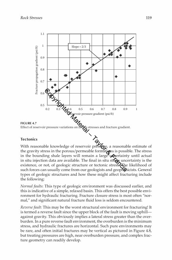
Of course, along with controlling the initial stress magnitude, changes in reservoir pressure will cause closure pressure to change. With depletion, closure pressure will decline, and with injection, closure pressure will rise. A simple derivative shows

∆∆σ βH

pK= − ≈( )1

23

(4.14)

in reasonable agreement with field data after water flood data from Salz as seen in Figure 4.7 (Salz, 1977).


119Rock Stresses

Tectonics

With reasonable knowledge of reservoir pressure, a reasonable estimate of the gravity stress in the porous/permeable formations is possible. The stress in the bounding shale layers will remain a large uncertainty until actual in situ injection data are available. The final in situ stress uncertainty is the existence, or not, of geologic structure or tectonic stress. The likelihood of such forces can usually come from our geologists and geophysicists. General types of geologic structures and how these might affect fracturing include the following:

Normal faults: This type of geologic environment was discussed earlier, and this is indicative of a simple, relaxed basin. This offers the best possible envi-ronment for hydraulic fracturing. Fracture closure stress is most often “nor-mal,” and significant natural fracture fluid loss is seldom encountered.

Reverse fault: This may be the worst structural environment for fracturing! It is termed a reverse fault since the upper block of the fault is moving uphill—against gravity. This obviously implies a lateral stress greater than the over-burden. In a pure reverse fault environment, the overburden is the minimum stress, and hydraulic fractures are horizontal. Such pure environments may be rare, and often initial fractures may be vertical as pictured in Figure 4.8, but treating pressures are high, near overburden pressure, and complex frac-ture geometry can readily develop.

0.20.5

0.6

0.7

0.8

0.9

1

1.1

0.3 0.4 0.5 0.6Reservoir pressure gradient (psi/ft)

Frac

ture

pro

paga

tion

grad

ient

(psi/

ft) Slope = 2/3

0.7 0.8 0.9 1

Figure 4.7Effect of reservoir pressure variations on in situ stresses and fracture gradient.



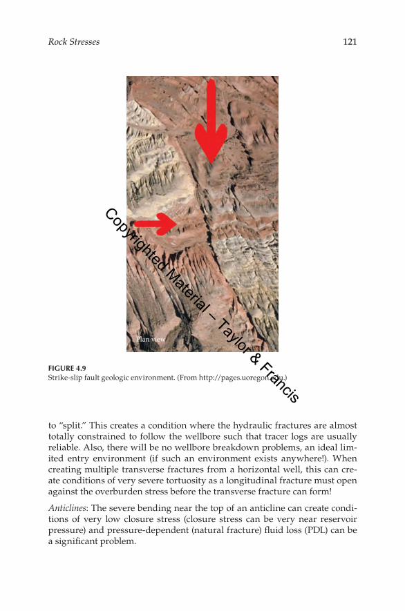
Strike-slip faults: For strike-slip faults, the stress situation is such that frac-tures are vertical and closure pressure is (or may be) “normal”; it is just that the fracture has a “strong,” preferred azimuth. In fact, one of the horizontal stresses is greater than the vertical stress. For this geologic structure, the major geologic faults will be vertical as seen in Figure 4.9 (a bird’s eye view of a strike-slip fault at the earth’s surface).

This can sometimes have indirect effects on hydraulic fracturing. For ver-tical wells, it can create “drilling-induced fractures” as seen in Figure 4.10, where the very high maximum horizontal stress causes the wellbore

(b)

σHmax

σv

(a)

Low angle“Thrust” fault

σ H min

Figure 4.8Thrust fault geologic environment. (a) Diagram of a log angle “thrust” fault. (b) Outcrop of a thrust fault. (From http://pages.uoregon.edu.)


121Rock Stresses

to “split.” This creates a condition where the hydraulic fractures are almost totally constrained to follow the wellbore such that tracer logs are usually reliable. Also, there will be no wellbore breakdown problems, an ideal lim-ited entry environment (if such an environment exists anywhere!). When creating multiple transverse fractures from a horizontal well, this can cre-ate conditions of very severe tortuosity as a longitudinal fracture must open against the overburden stress before the transverse fracture can form!

Anticlines: The severe bending near the top of an anticline can create condi-tions of very low closure stress (closure stress can be very near reservoir pressure) and pressure-dependent (natural fracture) fluid loss (PDL) can be a significant problem.

Plan view

Figure 4.9Strike-slip fault geologic environment. (From http://pages.uoregon.edu.)



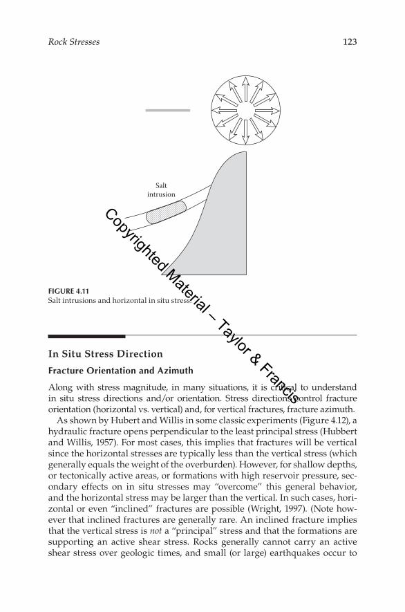
Salt: Salt has the unusual property that under geologic loads, it does not have stress—it has pressure (Talobre, 1957). That is, it flows and acts like a fluid. Thus, if we looked down on this salt diaper in Figure 4.11, the salt would be pressing outward on the sand layer with a pressure equal to the weight of the overburden. Thus, any attempt to initiate a hydraulic fracture in the vicinity of the salt will result in a vertical fracture that will orient itself perpendicular to the salt and will propagate in one direction only—toward the salt. The salt will act as a very strong magnet to attract the fracture. Since, in many frac-pack scenarios, an idea goal is to drill parallel to the salt right at the top corner of the reservoir, this can result in very poor frac-pack results (due to the fracture being transverse to the wellbore right at the top perforation, thus failing to place gravel over much of the perforated interval).

2434

2433

2432

2431

2430

2429

GRHCal

Resis PefRHOZ

UBI statamplitude

UBI dyncentered radius

UBI stat Top 3D view

CO 4

0.4

Dips

Figure 4.10Drilling-induced fractures.


123Rock Stresses

In SituStressDirection

Fracture Orientation and Azimuth

Along with stress magnitude, in many situations, it is critical to understand in situ stress directions and/or orientation. Stress directions control fracture orientation (horizontal vs. vertical) and, for vertical fractures, fracture azimuth.

As shown by Hubert and Willis in some classic experiments (Figure 4.12), a hydraulic fracture opens perpendicular to the least principal stress (Hubbert and Willis, 1957). For most cases, this implies that fractures will be vertical since the horizontal stresses are typically less than the vertical stress (which generally equals the weight of the overburden). However, for shallow depths, or tectonically active areas, or formations with high reservoir pressure, sec-ondary effects on in situ stresses may “overcome” this general behavior, and the horizontal stress may be larger than the vertical. In such cases, hori-zontal or even “inclined” fractures are possible (Wright, 1997). (Note how-ever that inclined fractures are generally rare. An inclined fracture implies that the vertical stress is not a “principal” stress and that the formations are supporting an active shear stress. Rocks generally cannot carry an active shear stress over geologic times, and small (or large) earthquakes occur to

Saltintrusion

Figure 4.11Salt intrusions and horizontal in situ stress.



relieve this shear stress. Thus, inclined fractures will be rare and will gener-ally be associated with areas of active tectonic activity.)

Knowledge of fracture azimuth will often be critical for low-permeability formations such as tight gas or shale gas since this controls fracture azimuth (Figure 4.13). This will then control well spacing for massive hydraulic fractur-ing and well spacing and well drilling direction of fractured horizontal wells.

The difference in stress/wellbore directions also plays a major role in “tortuosity,” a large near wellbore pressure drop due to flow restrictions (tortu-ous flow paths) between the wellbore and the main body of the fracture (with this flow restriction generated by some fracture complexity outside the steel).

A simple form of this would be a fracture that initiates along the wellbore and then turns as pictured in Figure 4.14. This produces a situation where the closure stress acting on the near wellbore fracture is greater than the minimum in situ stress. Thus, fracture width over the perforations is very narrow producing a flow restriction. The “local” closure stress over the per-forated interval is then given by

σ σ σ σ βCL Local H H H- = + −( )min max min sin ( )2 (4.15)

σHmin

σv=σmin

6

12

Figure 4.12Classic experiments on hydraulic fracturing. (After Hubbert, M.K. and Willis, D.G., Trans. Soc. Petrol. Eng., SPE 686, 210, 153, 1957.)


125Rock Stresses

This shows that for wellbore deviations (or azimuths different from orthogo-nal to the minimum in situ stress) up to 15°, the azimuth deviation has very little difference on anything regardless of the magnitude of the stress differ-ences. For example, even for a stress difference of 0.7 psi/ft versus 1.0 psi/ft at 10,000 ft (3,000 psi), the extra stress over the perforations would only be about 150 psi. This would probably not be sufficient to cause significant problems for most cases.

For angles greater than that, problems simply worsen, with magnitude of the problem related to the angle and the stress difference.

This is in line with the experimental results of Hallam and Last (1991). As seen in Figure 4.15, their results showed no imperfections in the fracture for deviations (or direction differences) of less than 10°.

Gooddrainage Poor

drainage

Low permeability—Loss of reservesdesign Xf < Re

σHmin

σHmax

Figure 4.13Azimuth/direction of vertical fractures controlled by orientation of horizontal stresses.



σHmin

σHmax

Poordrainage

Gooddrainage

Low permeability—Loss of reservesdesign Xf < Re

(a)

(c)

(b)

Plan view

Greater closure stress dueto non-favorable near well

fracture orientation

Minimumhorizontal

in situstressσHmin

Maximumhorizontal

in situstressσHmax

Preferred fractureAzimuth, vertical fracture

N

E

β

A vertical fracture may “turn” in thevicinity of a deviated well. However, theresulting non-favorable fractureorientation can result in a locally narrowfracture width. �is is probably stillgenerally preferable to multiple verticalfractures.

Figure 4.14Effect of well deviation (azimuth) on near wellbore “closure pressure.” (a) Orientation of a frac-ture in relation to the two horizontal stresses. (b) Diagram showing the relation of the fracture orientation to well placement for optimizing drainage. (c) Local near wellbore stress influence on fracture orientation.


127Rock Stresses

In SituStressDifferences

Differences between in situ stresses play a dominant role in hydraulic frac-ture behavior. In general, for “simple” fracture behavior, it is desirable to maintain the stress/pressure relation:

σ σCL CL NetBHTP P< = + <( ) Any other stress (4.16)

In this relation, “BHTP” is the bottom-hole treating pressure (or bottom-hole injection pressure) beyond the perforations and out in the main body of the fracture. Once the pressure inside the fracture begins to exceed the other in situ stresses, then fracture behavior is subject to change, and the fracture may become “complex.” That is, fracture height growth may start for a previously confined height fracture. If the BHTP exceeds the weight of the overburden, it may become possible to open a new horizontal frac-ture (i.e., “T”-shaped fractures), etc. Such a change in fracture geometry may occur late in a treatment and thus may have drastic effects on treatment pumping behavior.

00

10

20

30

40

50

60

70

80

90

10 20 30 40 50Well deviation (deg)

Experimental data

Diff

eren

ce in

azim

uth

from

pre

ferr

ed az

imut

h (d

eg)

60 70 80 90

Figure 4.15Critical well deviation/azimuth for “no” adverse effects (for a specific set of stress conditions). (After Hallam, S.D. and Last, N.C., J. Petrol. Technol., SPE 20656, 43, 742, 1991.)



Stress Barriers for Height Containment: ΔσShale–Sand

Along with the minimum stress in the “pay” zone controlling fracture ori-entation and azimuth—the difference in minimum stress between the pay and under-/overlying zones (ΔσShale–Sand) is most often the controlling param-eter for fracture height growth (for vertical fractures) (Warpinski, 1982). This is quantified in the “Fracture Height” section of Chapter 3. However, Figure 4.16 illustrates the large differences in stress that can occur from for-mation to formation. The different mechanical properties of the formations combined with geologic history have produced very large stress differences (up to 1500 psi) between the layers of this sand/shale sequence located in the Western United States (Warpinski, 1985).

Note in the figure that all the vertical variations in closure stress are asso-ciated with lithology changes. In general, a significant change in lithology (or pore pressure) is a necessary condition before one might expect signifi-cant variations in the stress state and thus fracture height confinement.

0

Sand

Sand

Silty

Shal

eSh

ale

50.00GR API

Cozz

ette

Man

cos

shal

e

Rolli

nsSS

Palu

dal

Neutron Stress psi

OB psiDensity

100 0

0

0.15

0.15

0.30

0.30

6000

6000

7500

7500

9000

9000

8000

7800

7600

7400

TVDft

Figure 4.16Changes in σHmin related to lithology. (After Warpinski, N.R., J. Petrol. Technol., SPE 8932-PA, 34, 653, 1982.)


129Rock Stresses

Stress Barriers for Height Containment—ΔσShale–Sand—How Big?

How large a stress difference can exist between different formations? In prin-ciple, there is no theoretical limit—though overburden stress might offer one practical limit for stress in a shale. For the case of significant reservoir pres-sure depletion, as an example, very large stress differences can be created as closure pressure in the permeable zone decreases. As a strictly empirical “rule of thumb,” for “virgin” formations, the maximum stress difference is usually less than 0.2 psi/ft of depth (0.00452 MPa/m).

Where does this rule come from? This is simply the largest in situ stress difference that has been measured and published (Figure 4.16) with a shale–sand stress difference of 1500 psi at about 7500 ft TVD. Other published data discussed in Chapter 7 shows measured stress differences smaller than this (near 0, 0.1, and 0.15 psi/ft difference), and in many situations, the stress differ-ence may be 0. In one instance (Shumbera, 2003), stress in an overlying shale was found to be less than the sand stress. The historical success of hydraulic fracturing probably argues that such a condition is a rare exception to the rule that shale formations (particularly clay-rich sale formations) have higher stress than porous/permeable sandstones and limestone.

Measured Stress Differences

A thorough literature review of petroleum and rock mechanics literature revealed 23 cases with measured values of sand/shale stresses. The shale–sand stress differences for these cases are summarized in Figure 4.17, with

0–0.050

1

2

Num

ber o

f for

mat

ions

3

4

5

6

7

8

0.05–0.10ΔσShale-sand (psi/ft)

Average 0.12 psi/ftMean 0.105 psi/ft

0.10–0.15 0.15–0.20 >0.25

Figure 4.17Shale–sand stress differences from multiple sources.



an average ΔσShale–Sand of 0.12 psi/ft (a mean of 0.10 psi/ft). Note that the value larger than 0.2 psi/ft is from the Wattenberg field. Virgin reservoir pressure in this field was about 0.38 psi/ft, slightly underpressured, creating a large shale–sand stress difference.

Secondary Fractures

Though the main hydraulic fracture will form, and open, perpendicular to the minimum in situ stress; special conditions can exist where a secondary, or auxiliary, fracture may open with an orientation or azimuth other than the preferred fracture geometry, that is, fracture complexity. Such an occur-rence is most likely in (1) shallow or overpressured wells where the differ-ence between horizontal and vertical stress is small, (2) deviated wells where the wellbore does not lie in the plane of the hydraulic fracture, and (3) tec-tonically active areas where the minimum stress may be neither horizontal nor vertical. The possible creation or opening of “secondary” fractures is also related to in situ stress differences. Also note that what are termed “second-ary fractures” here represent one form of “tortuosity,” that is, something lim-iting wellbore/fracture communication.

Secondary Fracture: “T” Fracture

Figure 4.18 illustrates possible auxiliary fracture geometry cases that could likely occur at shallower depths (or in overpressured reservoirs) where the difference between horizontal and vertical stress is relatively small. In this case, the pressure inside the fracture has exceeded overburden pressure.

Treating pressure in awell-confined vertical frac-

ture can become high enoughto lift the overburden andopen a horizontal fracture

Vertical+

horizontal

Figure 4.18Potential fracture complexity if BHTP > overburden.


131Rock Stresses

The fracture geometry cases pictured in these figures may (or may not) nor-mally create treatment pumping problems. However, by causing incorrect interpretation of post-frac logs or other data, the unusual geometry could lead to treatment designs that are unnecessarily large, or undesirably small. Also, treatment pumping problems are possible if the opening of the horizontal com-ponent of the fracture late in a treatment accelerates the near wellbore fluid loss.

The “case” of a vertical fracture with good height confinement is illustrated in Figure 4.18. As the fracture extends, the pressure (BHTP minus fracture closure stress) increases until, at some point, pumping pressure exceeds the weight of the overburden. At this point, a horizontal fracture could initi-ate along the top of the vertical fracture (at a shale–sand interface). In the worst case, the new, near wellbore fluid loss caused by the horizontal frac-ture could cause near well slurry dehydration and a premature screen-out. In the best (but probably rare) case, for naturally fractured formations or formations with good vertical permeability, the auxiliary horizontal fracture could significantly improve treatment results.

Secondary Fracture: Natural Fractures

Once a hydraulic fracture is created, it will tend to propagate along a single line—unless it encounters inhomogeneity in the formation such as natural fractures. If this occurs, the hydraulic fracture will tend to cross the natu-ral fractures so long as σHmax is significantly greater than σHmin. As the main hydraulic fracture continues to propagate, there may be some extra fluid loss to the natural fracture(s) (since even the mechanically closed natural frac-ture may have some preferential permeability); however, so long as pressure inside the hydraulic fracture remains below the stress holding the natural fracture closed, the extra loss should be minimal.

However, even if the magnitude of the extra fluid loss is significant, it will be a “normal” form of fluid loss. That is, the closed fracture will have a perme-ability, just as the formation matrix has a permeability, and this closed fracture permeability will contribute to increase the overall fluid loss. In this case, the natural fracture(s) would probably not have a significant impact on the treat-ment. However, once the treating pressure exceeds some critical level related to σHmax, the natural fracture will open, drastically altering the fluid loss and overall behavior of the hydraulic fracture. In this case, the fluid pressure inside the hydraulic fracture has exceeded the maximum horizontal stress.

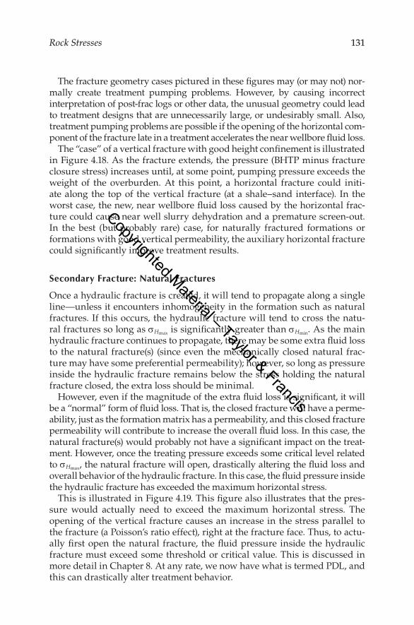
This is illustrated in Figure 4.19. This figure also illustrates that the pres-sure would actually need to exceed the maximum horizontal stress. The opening of the vertical fracture causes an increase in the stress parallel to the fracture (a Poisson’s ratio effect), right at the fracture face. Thus, to actu-ally first open the natural fracture, the fluid pressure inside the hydraulic fracture must exceed some threshold or critical value. This is discussed in more detail in Chapter 8. At any rate, we now have what is termed PDL, and this can drastically alter treatment behavior.



In SituStressMeasurement

Three techniques for measuring in situ stress exist, but only two are cur-rently in common use. These two are (1) injection tests and (2) long-spaced or dipole (shear wave) sonic logs. The third technique is strain measurements on core samples (Teufel, 1981). Advantages and disadvantages of these are discussed in the following. Generally, the best procedure is to perform a few direct stress (e.g., injection) tests in order to calibrate logs and/or core data. Logs can then be used to extrapolate the data vertically/horizontally.

injection Tests

Injection tests consist of perforating a short interval (typically 1–2 ft), iso-lating the zone with straddle packers (or a bridge plug and a packer), and breaking down the zone with a very small fluid volume (this can also be done in the open hole without the need for perforations). More discussion of field procedures and analysis techniques is included in Chapter 8. These tests are the only measurement that gives a “true” measurement for in situ stress. This is the “Catch 22” of fracturing! What do I need for designing a fracture treatment? I need to know the in situ stresses. How do I deter-mine in situ stress? That is easy. I hydraulically fracture the formation! Particularly for the elusive barrier (shale) stress—eventually we must pump to finally learn the truth!

σHmin

σHmax

σHmax

σHmax+Δσh

Δσh

Figure 4.19Potential fracture complexity if BHTP > σHmax.


133Rock Stresses

Shear Wave Sonic log Data

The use of log data for in situ stress was first applied by Rosepiler (1979) using long-spaced sonic logs to measure the shear and compressional velocity. These logs have been replaced with the current “dipole sonic log” where the dipole emitter emits a strong shear wave signal. In either case, the goal is to measure both the shear (VS) and compressional (VP) wave velocities. The ratio of these two velocities can be used to calculate a value for Poisson’s ratio using

ν =

( )( ) −

( ) −

1 2 1

1

2

2

/ ∆ ∆

∆ ∆

T T

T TS C

S C

/

/ (4.17)

where ΔTC and ΔTS are the compressional and shear wave travel times. This is used to calculate a K for the gravity–stress relation in Equation 4.7.

By inputting a value for pore pressure and overburden, and assuming tec-tonics is 0; fracture closure stress is calculated as

σ ν

νσ β βH V p p=

−− +

1( ) (4.18)

Given the simplicity of this calculation, there is clearly no sound theoreti-cal basis for the validity of this simple relation or for the use of dynamic elastic constants to represent behavior over geologic time. However, the log does offer a direct mechanical measurement of the formations, and reasonable correlated results have been found in several sand/carbonate/shale sequence-type reservoirs (Smith and Miller, 1989). One example of such a correlation is included in Figure 4.20 after Veatch (1982) along with

3,000

3,000

4,000

5,000

6,000

7,000

8,000

9,000

10,000

4,000 5,000 6,000Log stress (psi)

East TexasCotton Valley

Frontier

MesaVerde

CanyonSand

Real

stre

ss (p

si)

7,000 8,000 9,000

Figure 4.20Empirical relations between shear sonic log and measured σHmin.



other correlations. Note, however, that such a correlation is strictly local, log stresses can be either greater than or less than actual stresses.

ProppantStress

The final goals of a hydraulic fracture are fracture length (1/2 length or penetration, xf) and fracture conductivity (kfw). The conductivity part is strongly dependent on the stress acting on the proppant, and proppant conductivity is typically determined as a function of stress as discussed in Chapter 11. The stress acting to crush the proppant (the proppant stress) is given by

′ = + − −σ σ σ σProp CL Width CLBHFP t∆ ∆ ( ) (4.19)

whereΔσCL(t) is any decrease in closure stress due to reservoir pressure depletion. σ′ indicates that ′σProp is the effective stress on the proppant pack—the stress

actually acting to crush the proppant grains

Note that these data are often plotted as conductivity versus “closure stress” and that can be a dangerous over simplification.

Assuming that ΔσCL(t) is 0 (there is no decrease in closure stress due to depletion), the difference between proppant stress and closure stress lies in the two terms ΔσWidth and “BHFP.” ΔσWidth is an incremental stress acting on the proppant arising from the fact that the proppant is acting to hold the fracture open. That is, this proppant is prying the fracture open by a small amount, and that is reflected by a stress acting back on the proppant. This can be calculated (approximately) by

∆σ

π νWidth

PropEwH

=−

21 2( )

(4.20)

whereE is the Young’s modulus of the formation in units of psi or MPa giving a

corresponding value of ΔσWidth in psi or MPawProp and H are each in the same units of “length”

For most cases of normal modulus rock (say E < 3 × 106 psi, <2.1 × 104 MPa), the value of this extra stress is typically quite small, maybe 200 or 300 psi (1 or 2 MPa). Note that in the aforementioned equation, Poisson’s ratio is typically on the order of 0.2, and 0.2 squared is 0.04, so ν is not important to this calculation. At any rate, for many, many cases, ΔσWidth is on the order of 200 psi, while ′σProp is on the order of 1000s of psi. Thus, ΔσWidth can generally be ignored—at least in initial design planning.

The remaining parameter is “BHFP,” the bottom-hole producing pressure. To assume proppant stress equals closure stress assumes that BHFP is near


135Rock Stresses

0 before any significant reservoir depletion occurs. This may be a typical assumption for North American tight gas but is not a good assumption for many, maybe most other areas of the world.

WellboreBreakdown

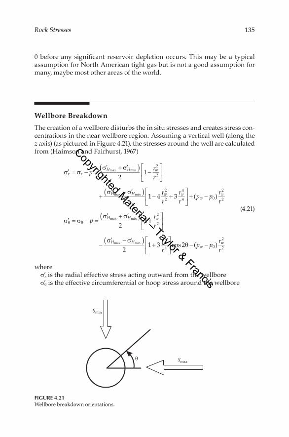
The creation of a wellbore disturbs the in situ stresses and creates stress con-centrations in the near wellbore region. Assuming a vertical well (along the z axis) (as pictured in Figure 4.21), the stresses around the well are calculated from (Haimson and Fairhurst, 1967)

′ = − =′ + ′( )

−

+′ − ′( )

−

σ σσ σ

σ σ

r rH H w

H H

prr

max min

max min

21

21 4

2

2

rrr

rr

p prr

p

w ww

w

H H

2

2

4

4 0

2

23

21

+

+ −

′ = − =′ + ′( )

( )

max minσ σσ σ

θ θ ++

−′ − ′( )

+

− −

rr

rr

p pr

w

H H ww

2

2

4

4 02

1 3 2σ σ

θmax min cos ( ) ww

r

2

2

(4.21)

where′σr is the radial effective stress acting outward from the wellbore′σθ is the effective circumferential or hoop stress around the wellbore

Smin

Smaxθ

Figure 4.21Wellbore breakdown orientations.



Limiting this to the wellbore wall (r = rw) simplifies this to

σ

σ σ σ σ σ θ

τ

θ

θ

r w

H H H H w

r

p p

p p

= −

= ′ + ′( ) − ′ − ′( ) − −

=

max min max min cos ( )2 2

00

(4.22)

and considering θ = 0 (the direction perpendicular to the minimum horizon-tal stress) yields

σ

σ σ σθ

r w

H H w

p p

p p

= −

= ′ − ′ − −3 min max ( ) (4.23)

Now fracture initiation occurs when the hoop stress equals to the tensile strength of the rock (−T here since compression is being treated as positive):

− = ′ − ′ − − = ′ − ′ + +T p p p p TH H w w H H3 3σ σ σ σmin max min max( ), (4.24)

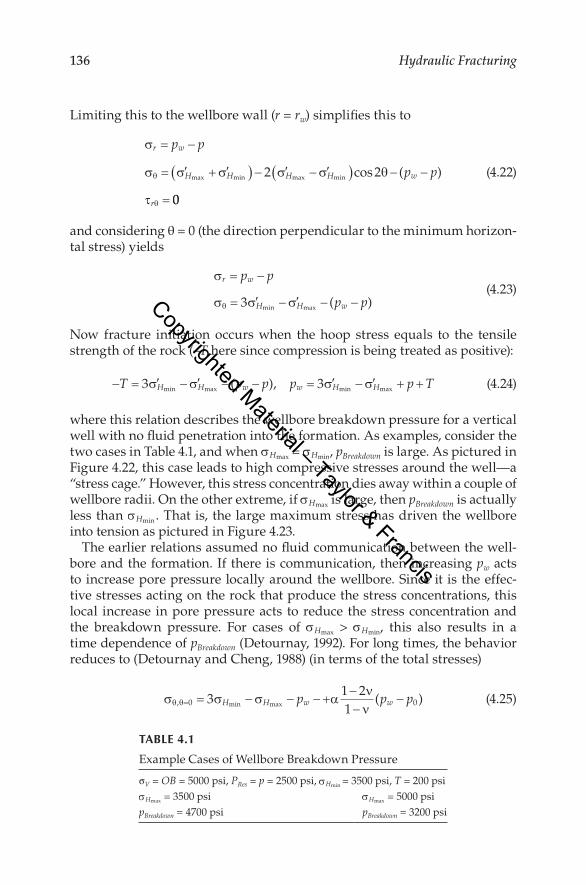
where this relation describes the wellbore breakdown pressure for a vertical well with no fluid penetration into the formation. As examples, consider the two cases in Table 4.1, and when σHmax = σHmin, pBreakdown is large. As pictured in Figure 4.22, this case leads to high compressive stresses around the well—a “stress cage.” However, this stress concentration dies away within a couple of wellbore radii. On the other extreme, if σHmax is large, then pBreakdown is actually less than σHmin . That is, the large maximum stress has driven the wellbore into tension as pictured in Figure 4.23.

The earlier relations assumed no fluid communication between the well-bore and the formation. If there is communication, then increasing pw acts to increase pore pressure locally around the wellbore. Since it is the effec-tive stresses acting on the rock that produce the stress concentrations, this local increase in pore pressure acts to reduce the stress concentration and the breakdown pressure. For cases of σHmax > σHmin, this also results in a time dependence of pBreakdown (Detournay, 1992). For long times, the behavior reduces to (Detournay and Cheng, 1988) (in terms of the total stresses)

σ σ σ α ν

νθ θ, min max ( )= = − − − + −

−−0 03

1 21

H H w wp p p (4.25)

TABle 4.1

Example Cases of Wellbore Breakdown Pressure

σV = OB = 5000 psi, PRes = p = 2500 psi, σHmin = 3500 psi, T = 200 psiσHmax = 3500 psi σHmax = 5000 psipBreakdown = 4700 psi pBreakdown = 3200 psi


137Rock Stresses

From Haimson and Fairhurst (1969), initiation then occurs when the effec-tive circumferential stress ( ′ = −σ σθ θ pw) equals the tensile strength, −T, of the rocks. This gives the initiation pressure of

σ σ σ σ α νν

θ θ θ θ, , min max ( )= = ′ + = − + = − − + −−

−

=

=0 00 31 21

p T p p p p

p

w w H H w w

w33 1 2 1

2 1 2 10σ σ α ν ν

α ν νH H T pmin max (( ) ( ))

( ) ( )− + − − −

− − −( )/

/

(4.26)

Smax

Smax = SminSmin

(a)

0.50.60.70.80.91.0

RW

PCL

“Extra” near-wellclosure stress

Closure stress along fracture azimuthp = 0.44 psi/ft, Smin = Smax = 0.7, RW = 4.5 in.

1.11.21.31.41.5

86 10Radius (in.)

Clos

ure p

ress

ure (

psi/f

t)

12 14(b)

Figure 4.22Wellbore “stress cage” for cases with σHmax approximately = σHmin. (a) Diagram of the stresses around a wellbore. (b) Relationship of the change in closure pressure vs. the radius of the wellbore.



wherep0 is the far-field reservoir pressureα is the Biot’s poroelastic parameterThe poroelastic term α(1 − 2ν)/(1 − ν) is typically equal to about 0.5

Equations 4.24 and 4.26 are then used to calculate the values in Figure 4.24.

Smin Smax>> Smin

Smax

Figure 4.23Wellbore “tension” for cases with σHmax ≫ σHmin.

00.4

0.5

0.6W/fluid penetration

No fluid penetration

0.7

0.8

0.9

1.0

1.1

1.2

1.3

1.4

2,000 4,000 6,000Depth (ft)

Brea

kdow

n gr

adie

nt (p

si/ft)

8,000 10,000 12,000

Figure 4.24Wellbore breakdown with and without fluid penetration.


139Rock Stresses

References

Biot, M. (1956). General solutions of the equations of elasticity and consolidation for a porous material. Journal of Applied Mechanics, 23, 91–96.

Breckels, I. M. (1981). Relationship between horizontal stress and depth in sedimen-tary basins. In SPE 10336, Presented at 1981 Annual Meeting of SPE. San Antonio, TX: SPE.

Brown, E. T. (1978). Trends in relationships between measured rock in situ stresses and depth. International Journal of Rock Mechanics and Mining Sciences & Geomechanics, 15, 211–215.

Detournay, E. and Cheng, A. H.-D. (1988). Poroelastic response of a borehole in a non-hydrostatic stress field. International Journal of Rock Mechanics and Mining Sciences & Geomechanics Abstracts, 25(3), 171–182.

Detournay, E. and Cheng, A. E. (1992). Influence of pressurization rate on the mag-nitude of the breakdown pressure. In Proceedings of the 33rd Symposium on Rock Mechanics (pp. 325–333). Santa Fe, New Mexico.

Eaton, B. A. (1969). Fracture gradient prediction and its application in oilfield opera-tions. SPE 2163, Journal of Petroleum Technology, 21, 1353–1360.

Haimson, B. and Fairhurst, C. (1967). Initiation and extension of hydraulic fractures in rocks. SPE 1710-PA, SPE Journal, 7, 310–318.

Haimson, B. and Fairhurst, C. (1969). Hydraulic fracturing in porous-permeable materials, Journal of Petroleum Technology, 21(7), 811–817.

Hallam, S. D. and Last, N. C. (1991). Geometry of hydraulic fractures from modestly deviated wellbores. Journal of Petroleum Technology, 43, 742–748.

Hubbert, M. K. and Willis, D. G. (1957). Mechanics of hydraulic fracturing—SPE 686, Petroleum Transaction, AIME, 210, 153–168.

Knappett, J. A. and Craig, R. F. (2012). Craig’s Soil Mechanics, Eighth Edition. Boca Raton, FL: CRC Press.

Rosepiler, M. J. (1979). Determination of principal stresses and confinement of hydrau-lic fractures in cotton valle. In SPE 8405-MS, SPE Annual Technical Conference and Exhibition. Las Vegas, NV: SPE.

Salz, L. B. (1977). Relationship between fracture propagation pressure and pore pres-sure. In SPE 6870, Presented at 52nd Annual Fall Meeting of SPE. Denver, CO: SPE.

Shumbera, D. A. (2003). Design and long-term production performance of frac pack completions in a Gulf of Mexico deepwater turbidite field having inverted sand-shale stress. In SPE 84259, Prepared for Presentation at the SPE Annual Technical Conference and Exhibition. Denver, CO: SPE.

Smith, M. B. and Miller, W. K. Reanalysis of the MWX fracture stimulation data from the paludal zone of the Mesaverde Formation, SPE Annual Technical Conference and Exhibition, San Antonio, TX, 1989.

Talobre, J. (1957). La Mécanique des Roches. Paris, France: Dunod.Teufel, L. W. (1981). Strain relaxation method for predicting hydraulic fracture

azimuth from oriented core. In SPE 9836, SPE/DOE Low Permeability Gas Reservoirs Symposium. Denver, CO: SPE.

Veatch Jr., R. W. (1982). Joint research/operations programs accelerate massive hydraulic fracturing technology, SPE 9337-PA. Journal of Petroleum Technology, 34, 2763–2775.



Warpinski, N. B. (1985). In-situ stress measurements at the DOE’S multiwell experi-ment site, Mesaverde Group, Rifle, Colorado, SPE 12142. Journal of Petroleum Technology, 37, 527–536.

Warpinski, N. R. (1982). In-situ stresses: The predominant influence on hydraulic fracture containment, SPE 8932-PA. Journal of Petroleum Technology, 34, 653–664.

Wright, C. A. (1997). Horizontal hydraulic fractures: Oddball occurrences of practical engineering concern? In SPE 38324, SPE Western Regional Meeting, Long Beach, CA, June 25–27, 1997.


rock stresses - crc press online · 2020-03-23 · rock stresses 115 of that expansion is governed...

Documents